The Energy Sources, the Physical Properties, and the Mass-loss History of SN 2017dio
Abstract
We study the energy sources, the physical properties of the ejecta and the circumstellar medium (CSM), as well as the mass-loss history of the progenitor of SN 2017dio which is a broad-lined Ic (Ic-BL) supernova (SN) having unusual light curves (LCs) and signatures of hydrogen-rich CSM in its early spectrum. We find that the temperature of SN 2017dio began to increase linearly about 20 days after the explosion. We use the 56Ni plus the ejecta-CSM interaction (CSI) model to fit the LCs of SN 2017dio, finding that the masses of the ejecta, the 56Ni, and the CSM are 12.41 M⊙, 0.17 M⊙, and 5.82 M⊙, respectively. The early-time photosphere velocity and the kinetic energy of the SN are respectively 1.89 km s-1 and 2.66 erg, which are respectively comparable to those of SNe Ic-BL and hypernovae (HNe). We suggest that the CSM of SN 2017dio might be from an luminous-blue-variable-like outburst or pulsational pair instability 1.211.4 yr prior to the SN explosion, or binary mass transfer. Moreover, we find that its ejecta mass is larger than those of many SNe Ic-BL, and that its 56Ni mass () is approximately equal to the mean (or median) value of of SNe Ic-BL in the literature, but lower than of prototype HNe (e.g., SN 1998bw and SN 2003dh).
1 Introduction
Core-collapse supernovae (CCSNe) are from the explosions of massive stars whose Zero Age Main Sequence (ZAMS) masses are larger than 8 M⊙. The explosions leave neutron stars or black holes in their centers. According to their spectra, most CCSNe can be divided into types II, IIb, Ib, and Ic (Filippenko, 1997). SNe II retain hydrogen envelopes before explosions; SNe Ib lost hydrogen envelopes before explosions; SNe Ic lost hydrogen and almost all helium envelopes before explosions (Filippenko, 1997). A minor fraction of SNe Ic are broad-lined ones (SNe Ic-BL) whose absorption lines in spectra are broader than those of normal SNe Ic. The derived photospheric velocities of many SNe Ic-BL are km s-1 (see, e.g., Woosley & Bloom 2006, Hjorth & Bloom 2012 , and references therein), which are significantly higher than those of normal SNe Ic (Woosley & Bloom, 2006). Moreover, some SNe Ic-BL have kinetic energy () erg, becoming hypernovae (HNe, e.g., Iwamoto et al. 1998; Iwamoto et al. 2000). 111Paczyński (1998) propose the term ”hypernova” to name the explosive phenomenon (especially for the luminous optical afterglows associated with observed gamma-ray bursts) that is much more luminous and energetic than any SN. Following studies modeling SNe Ic-BL (e.g., Iwamoto et al. 1998; Iwamoto et al. 2000) use ”hypernova” to name the SNe that are much more energetic than normal SNe which have kinetic energy erg. Most HNe have kinetic energy erg (see, e.g., Iwamoto et al. 1998; Iwamoto et al. 2000, Table 9.2 of Hjorth & Bloom 2012 and references therein). It is widely believed that the main energy of the light curves (LCs) of most SNe Ib and Ic (including SNe Ic-BL and HNe) are from the cascade decay of the synthesized 56Ni by the SNe (e.g., Arnett 1982; Cappellaro et al. 1997; Valenti et al. 2008; Drout et al. 2011; Cano 2013; Taddia et al. 2015; Wheeler et al. 2015; Lyman et al. 2016; Prentice et al. 2016; Taddia et al. 2019).
In the past four decades, a few hundred interacting CCSNe (Smith, 2017) with narrow and intermediate-width emission lines indicative of the interaction between the ejecta and circumstellar medium (CSM) have been confirmed (e.g., Schlegel 1990; Mattila et al. 2008; Pastorello et al. 2008a, b, 2016; Fraser et al. 2021; Perley et al. 2022; Gal-Yam et al. 2022; Davis et al. 2023). It is believed that the emission lines are produced by the ejecta-CSM interaction (CSI) (Schlegel, 1990; Filippenko, 1997). According to the features of their spectra, interacting CCSNe can be divided into types IIn (Schlegel, 1990), Ibn (Mattila et al., 2008; Pastorello et al., 2008a, b, 2016), and Icn (Fraser et al., 2021; Perley et al., 2022; Gal-Yam et al., 2022; Davis et al., 2023). The three subclasses respectively show hydrogen emission lines, helium emission lines, and helium-deficient emission lines, indicating the existence of hydrogen-rich (for SNe IIn), helium-rich (for SNe Ibn), and helium-deficient (for SNe Icn) CSM.
The forward and reverse shocks produced by the CSI accelerate the electrons. Accelerated electrons emit high-energy (-ray and X-ray) photons, which can be thermalized to be UV-optical-IR photons if the densities of CSM are large enough. The emission produced by the CSI can provide additional or main energy source for powering the LCs of the interacting SNe (Chevalier, 1982; Chevalier & Fransson, 1994).
SN 2017dio is a peculiar interacting SN (Kuncarayakti et al., 2018) which was discovered on April 26, 2017 and then confirmed to be an SN Ic in the galaxy SDSS J113627.76+181747.3 whose redshift is 0.037 (see Kuncarayakti et al. 2018 and references therein). The follow-up observations performed by Kuncarayakti et al. (2018) obtain the optical () and near-infrared (NIR) () LCs of SN 2017dio. The early-time LCs of SN 2017dio are featured by the rising episodes with dips or short plateaus, while the late-time LCs are slow-evolving second peaks (see Figure 2 of Kuncarayakti et al. 2018). Based on the analysis for spectra, Kuncarayakti et al. (2018) find that SN 2017dio is an SN Ic-BL showing H emission lines , and conclude that it is the first confirmed SN Ic having signatures of hydrogen-rich CSM in the early spectrum. The feature of the spectral evolution of SN 2017dio is different to that of normal SN Ic (including SN Ic-BL) whose spectra do not show CSI signatures and that of SNe Icn which collide with hydrogen and helium-deficient CSM. On the other hand, the main features of SN 2017dio are reminiscent of SN 2017ens which is a superluminous SN (SLSN) showing the transition from an SN Ic-BL to an SN IIn (Chen et al., 2018).
The early-time LCs of SN 2017dio are well consistent with the template LCs of SNe Ic (Kuncarayakti et al., 2018), indicating that they might be powered by 56Ni cascade decay; the rebrighening of the LCs and the H emission lines in the spectra favor the scenario that the late-time LCs are mainly powered by CSI between the ejecta of SN 2017dio and the hydrogen-rich CSM surrounding the SN progenitor (Kuncarayakti et al., 2018).
The observations and detailed modeling for the constructed bolometric LC of SN 2017ens are performed by Chen et al. (2018). For comparison, the physical properties of the ejecta, the CSM, and the mass-loss history of the progenitor of SN 2017dio have not been quantitatively constrained, though the observations and some excellent analyses are performed by Kuncarayakti et al. (2018).
We suggest that the physical properties of SN 2017dio and the CSM surrounding the SN deserve further study, since the detailed modeling would reveal the energy sources, physical properties of the SN ejecta and the CSM, as well as the mass-loss history of the SN progenitor. Hence, we perform a detailed modeling for its multi-band LCs. In Section 2, we constrain the physical properties of SN 2017dio as well as the CSM by using the 56Ni plus CSI model to fit its multi-band LCs. In Section 3, we discuss the possible mechanism of the mass loss, infer the mass-loss history of the progenitor, and compare the physical properties of SN 2017dio to those of SN 2017ens and other SNe Ic-BL. In Section 4, we draw some conclusions. Throughout the paper, we assume , , and km s-1 Mpc-1 (Planck Collaboration, 2014). The values of the Milky Way reddening () are from Schlafly & Finkbeiner (2011).
2 Modeling the Multi-band Light Curves of SN 2017dio Using the 56Ni Plus CSI Model
As pointed out by Kuncarayakti et al. (2018), the early-time LCs which include the first peaks of SN 2017dio resemble those of SNe Ic (see template match using SNe Ic LCs in Figure 2 of Kuncarayakti et al. 2018) which are powered by 56Ni cascade decay, while the rebrightening LCs and prominent hydrogen and helium emission features in the spectra at the epochs after the first peaks suggest that the second peaks of the LCs of SN 2017dio might be powered by 56Ni cascade decay plus CSI.
Hence, we use the 56Ni plus CSI model to fit the LCs of SN 2017dio and assume the onset time of the CSI is later than that of 56Ni cascade decay. The time interval is set to be the difference between the onset time of CSI and the time of the first photometric point () minus the explosion time relative to the first data (), i.e., .
The 56Ni model we use to reproduce the bolometric LC is from equations (1) and (5) of Wang et al. (2023), which is based mainly on Arnett (1982) and Valenti et al. (2008); 222Arnett (1982) don’t consider energy from the process of 56Co to 56Fe and the leakage effect of -ray and positions; Valenti et al. (2008) include the 56Co to 56Fe process and the leakage effect. the equations of the CSI model used here can be found in Wang et al. (2019), which is based on Chevalier (1982), Chevalier & Fransson (1994), and Chatzopoulos et al. (2012). 333Wang et al. (2019) assume stationary photospheres at the early-time epochs, while we assume that the photosphere expanded at the early-time epochs. Both cases are considered in Section 2 of Chatzopoulos et al. (2012).
The density of CSM can be written as
| (1) |
where
| (2) |
here, is the innermost radius of the CSM, is the density of the CSM at . The power law index () is assumed to be 0, since Kuncarayakti et al. (2018) suggest that the CSM might be a shell whose density is constant at different radii; therefore, . The optical opacity () of the hydrogen-deficient ejecta and the hydrogen-rich CSM are set to be 0.07 (e.g., Taddia et al. 2015) and 0.34 cm2 g-1, respectively; the -ray opacity () and the opacity () are fixed to be 0.027 cm2 g-1 (e.g., Cappellaro et al. 1997; Mazzali et al. 2000; Maeda et al. 2003) and 7 cm2 g-1 (Cappellaro et al. 1997), respectively.
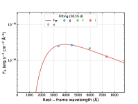
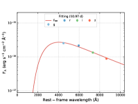
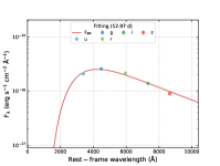
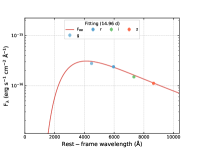
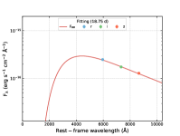
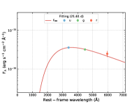
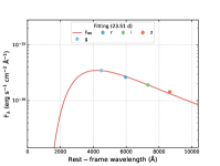
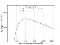
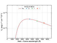
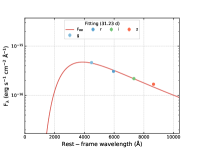
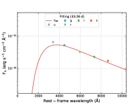
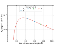
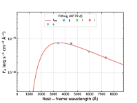
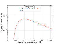
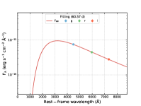
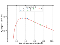
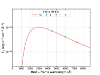
To fit the multi-band LCs, a photosphere modulus is needed. By using the blackbody model (, where and are the radius and temperature of SN photosphere, is the SN luminosity distance) to fit the optical-NIR SEDs at all epochs having photometry in at least three bands (see Figure A1, the corresponding best-fitting parameters are listed in Table A1), we find that the derived bolometric LC (the top-left panel of Figure 1) shows a dip (days 9 to 15 after the time of the first photometric data) and a slow-evolving second peak (days 60 to 90), which are consistent to the features of the multi-band LCs. Additionally, it can be found that the early-time velocity of the photosphere of the SN was approximately constant (the top-right panel of Figure 1), while the temperature of the SN increased linearly about 20 days after the explosion (the bottom panel of Figure 1).
Therefore, we assume that the evolution of photosphere radius can be described by Equation (9) of Nicholl et al. (2017), while the temperature evolution can be described the equation below
| (5) |
is the lowest photosphere temperature. This introduces two new free parameters, which is the time when the temperature began to increase and which is the slope of the temperature curve after .
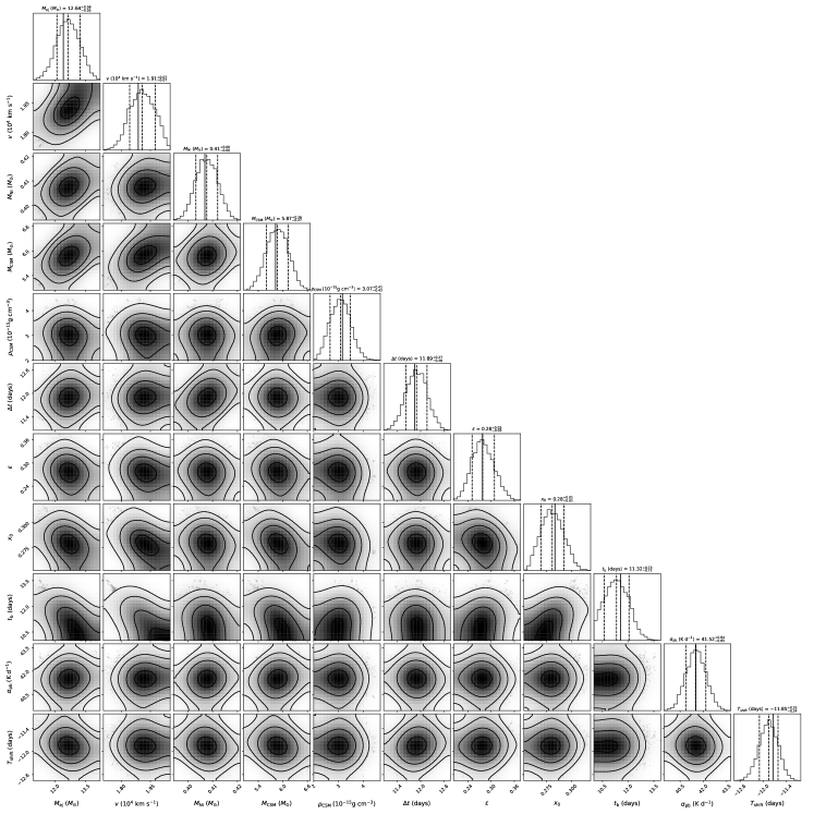
The definitions, the units, and the prior ranges of the parameters of the 56Ni plus CSI model are shown in Table 1. The Markov Chain Monte Carlo (MCMC) using the emcee Python package (Foreman-Mackey et al., 2013) is adopted to get the best-fitting parameters and the 1- bounds (which are corresponding to the 16th and 84th percentiles of the posterior samples) of the parameters.
All available photometric data which are in and bands are from Kuncarayakti et al. (2018), except for one upper limit (-band) and two data points (- and - bands) which are from the Asteroid Terrestrial-impact Last Alert System (ATLAS; Tonry 2011) and the Panoramic Survey Telescope and Rapid Response System (Pan-STARRS, PS1, Flewelling et al. 2020). 444https://www.wis-tns.org/object/2017dio The fitting of the LCs of SN 2017dio using the 56Ni plus CSI model is shown in Figure 2, the best-fitting parameters are listed in Table 1, the corresponding corner plot is presented in Figure A2. It can be found that the first peaks of SN 2017dio can be fitted by 56Ni model; the LCs would decline after the first peaks (see the dash-dotted lines of Figure 2) if the CSI was absent. The contribution of the CSI between the ejecta and the CSM (see the dashed lines of Figure 2) results in the rebrightening of the LCs.
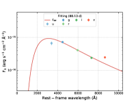
The last optical-NIR photometry (at 88.13 day) cannot be fitted by the model (the and band data deviate from the theoretical LC), since the optical-NIR SED at this epoch deviates from blackbody model (see the last panel of Figure A1). The photometry at the last epoch when only NIR data is available also can not be fitted by the model; the and band flux is higher than the theoretical LC, indicating that there might be NIR excess at this epoch.
The best-fitting parameters of the 56Ni plus CSI model are = 12.41 M⊙, = 1.89 km s-1, = 0.41 M⊙, = 5.82 M⊙, = 3.16 g cm-3, = 11.84 days, = 0.28, = 0.28, = 11.57 days, = 41.50 K d-1, days. The values of reduced (/dof, dof is the degree of freedom) is 114.48.
It should be noted that, however, Arnett (1982)’s model and it’s generalized versions (including the one we adopt) would overestimate the 56Ni masses of stripped-envelope SNe (including SNe Ic and Ic-BL) (see, e.g., Khatami & Kasen 2019). Thus we calculate more accurate value of 56Ni mass of SN 2017dio using the equation below (Khatami & Kasen, 2019)
| (6) |
The value of is 0.56 for SNe Ic-BL (Afsariardchi et al., 2021). Using the peak luminosity () and the rise time () of the bolometric LC produced by the best-fitting parameters of the multi-band LC fit, we find that the of SN 2017dio is 0.17 M⊙.
Assuming that the CSI was triggered when the LCs began to rebrighen, the time interval () from SN explosion to the time when CSI was triggered (; days, days, see Table 1) is 23.58 days. This value is about 1/3 times the value ( 80 days) inferred by Kuncarayakti et al. (2018) which assume that the CSI was triggered when H luminosity reached its peak. Using our derived photometric velocity ( km s-1) which is about twice that adopted by Kuncarayakti et al. (2018) ( km s-1) 555The value of Kuncarayakti et al. (2018) is from the mean value of SNe Ibc in Cano (2013). Note that the average values of SNe Ib, Ic, and SNe Ic-BL are km s-1, km s-1, and km s-1, respectively (see, e.g., Table D1 of Cano 2013). We suggest that the mean value of of SNe Ic-BL is more reasonable for SN 2017dio, since it is a SN Ic-BL., the derived value of the innermost radius of CSM () is cm (257 au), which is about half of the inferred value of Kuncarayakti et al. (2018) ( 500 au).
Combining the equation and the derived values of , , and , we find that the outermost radius and the thickness (, ) of the CSM are 9.37 cm (625 au) and 5.52 cm (368 au), respectively.
3 Discussion
3.1 The Mechanism and History of the Mass loss of the Progenitor
Kuncarayakti et al. (2018) exclude the possibility that the CSM of SN 2017dio is a steady-state stellar wind, and favor the scenario that the CSM is a shell expelled by the SN progenitor itself or from the binary companion.
The eruptions of massive stars can be triggered by the luminous-blue-variable (LBV)-like outbursts (Smith et al., 2011) or the pulsational pair instability (PPI) (Woosley et al., 2007; Woosley, 2017; Marchant et al., 2019; Renzo et al., 2020).
For the LBV-like outburst scenario, the derived CSM mass ( 5.82 M⊙) is in the range of the masses of CSM from LBV-like outbursts (0.01 to 10 M⊙, Smith et al. 2011). Assuming that the compact remnant is a neutron star with mass M⊙or a stellar mass black hole, the mass of the progenitor of SN 2017dio is 19.6 M⊙( M⊙). The ZAMS mass of the progenitor must be larger than this value, because the wind can reduce the mass of the progenitor. Smith et al. (2011) find that the initial (i.e., ZAMS) masses of some SN impostors which are related to the eruptions of massive hydrogen-rich stars are in the range of M⊙, which is significantly lower than the expected the range of ZAMS masses that can experience violent eruptions. This suggests that the ZAMS masses of massive stars that can trigger LBV-like eruptions can be down to 10 M⊙or even below 8 M⊙(Smith et al., 2011). Our derived progenitor mass of SN 2017dio ( 19.6 M⊙) indicates that it can experience LBV-like eruption.
For the PPI scenario, the derived CSM mass is comparable with the values derived in the literature (see, e.g., Table 2 of Liu et al. 2018, Extended Data Table 1 of Lin et al. 2023) using this scenario. The fact that the CSM of SN 2017dio is hydrogen-rich suggests that the metallicity () of the progenitor of SN 2017dio might be lower than those of the progenitors of type I SNe (e.g., SN 2017egm) whose progenitors are assumed to experience PPI, since it retained a moderate amount of hydrogen envelope prior to the PPI. 666The wind mass-loss rate of stars is proportional (Kudritzki et al., 1987; Leitherer et al., 1992; Vink et al., 2001; Mokiem et al., 2007), (Vink et al., 2001) or (Mokiem et al., 2007). It is more difficult to deplete the hydrogen envelopes via winds for low stars. Table 2 of Woosley (2017) lists the low metallicity () PPI models. For T80, T80A, T80B, T80C, and T80D Models in which the outbursts might correspond to type IIn SNe or SN impostors (Woosley, 2017) , the masses of the hydrogen envelopes of the pre-SN cores are in the range of 16.0943.6 M⊙; it can be expected that a higher would result in a lower hydrogen envelope mass before the PPI. our derived CSM mass might be reasonable, if the progenitor had a higher and/or experienced more than one outburst. In this scenario, the mass of the remnant is M⊙, since the masses of the pre-SN helium cores of T80, T80A, T80B, T80C, and T80D Models which can be set to be the upper limit of the progenitor mass just before the core collapse are in the range of M⊙ (see Table 2 of Woosley 2017), while the ejecta mass is M⊙. On the other hand, the lower limit of mass of the remnant is M⊙which corresponds to the extreme case that all the 5.82 M⊙of CSM is helium. Therefore, the remnant might be a black hole with mass in the range of M⊙.
We can infer the mass-loss history of the progenitor of SN 2017dio, if the CSM was expelled by an eruption of the progenitor shortly before the SN explosion. Smith et al. (2011) find that the velocities of hydrogen-rich CSM associated with SN impostors are in the range of km s-1 (see also Table 9 of Smith et al. 2011). On the other hand, Woosley (2017) points out that the typical velocity of the shells expelled by PPI are 200-800 km s-1 for Model T80A and 300-1000 km s-1 for Models T80B, T80C, and T80D; it is reasonable to assume that the velocity of the shell expelled by PPI is 200-1000 km s-1. Hence, we assume that is km s-1. Using ( is the time interval from the shell expelled to SN explosion,), we find the value of is days ( yr). Therefore, the progenitor of SN 2017dio might experience an eruption 1.211.4 yr prior to the SN explosion.
For the binary star scenario, the mass transfer rate of massive stars via Roche-lobe overflow (RLOF) can be of order M⊙yr -1 or higher (Taam & Sandquist, 2000; Langer, 2012; Smith, 2014), while the thermal (Kelvin-Helmholtz) timescale of the envelope is yr (Smith 2014, the value of can be estimated by using Equation 10 of Paczyński 1971). Using , the mass transferred can be up to M⊙or higher. Our derived CSM mass value is in the range of the mass transferred in binary systems.
3.2 Comparison With SN 2017ens
The main features of SN 2017dio resemble those of SN 2017ens which is an SLSN Ic. The spectra of SN 2017ens at 1 month after peak show some broad features which resemble those of SNe Ic-BL at similar epochs, while its late-time spectra indicate that it became an SN IIn (Chen et al., 2018). Although the spectral evolution of SN 2017dio and SN 2017ens share similar features, they also show some discrepancies.
(1). The bolometric luminosity of the first peak of SN 2017dio ( erg s-1) is lower than that of its second peak ( erg s-1), while the bolometric luminosity of the peak of SN 2017ens ( erg s-1, Chen et al. 2018) is higher than that of its late-time plateau ( erg s-1, see the bottom panel of Figure 1 of Chen et al. 2018).
(2). The peak bolometric luminosity of SN 2017ens is 10 times that of the bolometric luminosity of the first peak of SN 2017dio. Chen et al. (2018) demonstrate that the 56Ni model cannot account for the first peak of SN 2017ens, but the magnetar/fallback plus CSI model can explain it. In contrast, our modeling shows that the 56Ni model can explain the first peak of SN 2017dio. Without a central engine (magnetar or fallback) or CSI, the peak luminosity of SN 2017ens might be comparable to that of the first peak of SN 2017dio.
(3). The bolometric luminosity of plateau of the SN 2017ens is 1/5 times that of the second peak of SN 2017dio, indicating that the contribution of CSI between the ejecta of SN 2017dio and its CSM is higher than that of SN 2017ens.
(4). Based on the scenario that the early-time peak of SN 2017ens was powered mainly by a magnetar or fallback, Chen et al. (2018) suggest that the innermost radius of CSM of SN 2017ens is 1.2 cm. This value is 1/3 times that of SN 2017dio (3.85 cm).
3.3 Comparison With Other Broad-lined Type Ic SNe and HNe
Based on the best-fitting parameters derived, we can compare the physical properties of SN 2017dio to several prototype SNe Ic-BL and HNe whose physical properties had been comprehensively studied in the literature. The main parameters of the SNe Ic-BL and HNe are listed in Table 2.
The derived photospheric velocity () of SN 2017dio is 1.89 km s-1, which is comparable to other SNe Ic-BL (e.g., SN 1997ef, SN 2006aj, see Table 2), and favored by Kuncarayakti et al. (2018)’s conclusion that SN 2017dio is an SN Ic-BL. The ejecta mass of SN 2017dio (12.41 M⊙) is larger than those of HNe in Table 2. In the single-star framework, this might indicate that the progenitor of SN 2017dio had a ZAMS mass larger than those of HNe or a lower metallicity 777Having the same ZAMS masses, single stars with lower metallicity would result in lower and larger pre-SN masses, see footnote 6 for details., or produced a lighter compact remnant. In the binary framework, a higher ejecta mass might suggest that less material of the progenitor was accreted by the companion, and a more massive pre-SN core was left just prior to the SN explosion.
Using the equation , we find of SN 2017dio is 2.66 erg. This indicates that SN 2017dio might also be an HN. The value of of SN 2017dio is comparable to those of prototype HNe (e.g., SN 1998bw and SN 2003dh), and higher than that of SN 1997ef which is also an HN (see Table 2).
The value of of SN 2017dio is smaller than those of SN 1998bw and SN 2003dh, but comparable to that of SN 1997ef (see Table 2). Moreover, the 56Ni mass (0.17 M⊙) of SN 2017dio is approximately equal to the mean and median values (0.15 M⊙) of SNe Ic-BL reinvestigated by Afsariardchi et al. (2021). The value is also smaller than the median value (0.26 M⊙) of SNe Ic-BL studied by Cano (2013) as well as the median value (0.292 M⊙) of SNe Ic-BL in the Palomar Transient Factory (PTF; Rau et al. 2009; Law et al. 2009) sample studied by Taddia et al. (2019). As mentioned above, however, Arnett (1982)’s model which was also used by Cano (2013) and Taddia et al. (2019) would overestimate the of stripped-envelope SNe (including SNe Ic-BL); using equation 6, the medians of of SNe Ic-BL can be reduced by a factor of 0.5, and comparable to those of Afsariardchi et al. (2021) and the derived of SN 2017dio.
4 Conclusions
SN 2017dio is an SN Ic-BL that had been confirmed to interact with CSM by its spectral evolution and the LC rebrightening. In this paper, we study the energy sources as well as the physical properties of the SN and the CSM surrounding the SN progenitor.
We use the 56Ni plus CSI model and blackbody model to fit the multi-band LCs of SN 2017dio. A new photospheric modulus assuming a linearly increasing temperature evolution is adopted since the fitting for the optical-NIR SEDs at different epochs demonstrate that its temperature evolution linearly increased about 20 days after the explosion.
We find that the ejecta mass, the 56Ni mass, and the CSM mass are 12.41 M⊙, 0.17 M⊙, and 5.82 M⊙, respectively. The early-time photosphere velocity and the kinetic energy of the SN are respectively 1.89 km s-1 which is comparable to those of SNe Ic-BL and 2.66 erg which is comparable to those of HNe. Therefore, SN 2017dio might be an HN embedded in a hydrogen-rich CSM. By comparing the derived parameters of SN 2017dio to those of SNe Ic-BL and HNe in the literature, we find that the ejecta mass of SN 2017dio is larger than those of many SNe Ic-BL and HNe; the derived 56Ni mass of SN 2017dio is approximately equal to the mean (or median) value of those of SNe Ic-BL and SN 1997ef which is an HN, but lower than the 56Ni masses of prototype HNe (SN 1998bw and SN 2003dh).
The CSM can be from an eruption of the progenitor of SN 2017dio or the companion of the progenitor via the mass transfer process. In the single-star framework, we find that the progenitor experience an eruption expelling a shell 1.211.4 yr prior to the SN explosion, if the eruption was caused by an LBV-like outburst or PPI. The derived CSM mass is comparable with the values derived in the literature adopting the two scenarios, indicating that the CSM of SN 2017dio might be expelled by an eruption caused by an LBV-like outburst or PPI. In the binary framework, the derived CSM mass is lower than the upper limit ( 10 M⊙) of the transferred mass in binary systems.
By comparing the LCs and energy sources of SN 2017dio to those of SLSN SN 2017ens, we find that SN 2017dio and SN 2017ens show some differences, though the spectral evolution of the two SNe are similar. The most prominent difference is that the peak luminosity of SN 2017ens, which is 10 times that of the first peak of SN 2017dio, cannot be explained by the 56Ni model; a central engine (a magnetar or fallback) or CSI is needed to account for the high luminosity of the first peak of SN 2017ens. For comparison, the first peak of SN 2017dio can be well explained by the 56Ni model. We suggest that the peak of SN 2017ens might be comparable to that of the first peak of SN 2017dio, if the putative central engine (magnetar or fallback) or CSI was absent. In other words, the first peak of SN 2017dio can reach significantly higher luminosity if it was boosted by a central engine.
To date, SNe with LCs and spectral evolution like SN 2017dio and SN 2017ens are very rare. The upcoming sky surveys for SNe, follow-up observations as well as detailed modeling can shed light on the nature of them.
References
- Afsariardchi et al. (2021) Afsariardchi, N., Drout, M. R., Khatami, D. K., et al. 2021, ApJ, 918, 89
- Arnett (1982) Arnett, W. D. 1982, ApJ, 253, 785
- Cano (2013) Cano, Z. 2013, MNRAS, 434, 1098
- Cappellaro et al. (1997) Cappellaro, E., Mazzali, P. A., Benetti, S., et al. 1997, A&A, 328, 203
- Chatzopoulos et al. (2012) Chatzopoulos, E., Wheeler, J. C., & Vinko, J. 2012, ApJ, 746, 121
- Chen et al. (2018) Chen, T.-W., Inserra, C., Fraser, M., et al. 2018, ApJ, 867, L31
- Chevalier (1982) Chevalier, R. A. 1982, ApJ, 258, 790
- Chevalier & Fransson (1994) Chevalier, R. A. & Fransson, C. 1994, ApJ, 420, 268
- Davis et al. (2023) Davis, K. W., Taggart, K., Tinyanont, S., et al. 2023, MNRAS, 523, 2530
- Deng et al. (2005) Deng, J., Tominaga, N., Mazzali, P. A., et al. 2005, ApJ, 624, 898.
- Drout et al. (2011) Drout, M. R., Soderberg, A. M., Gal-Yam, A., et al. 2011, ApJ, 741, 97
- Filippenko (1997) Filippenko, A. V. 1997, ARA&A, 35, 309
- Flewelling et al. (2020) Flewelling, H. A., Magnier, E. A., Chambers, K. C., et al. 2020, ApJS, 251, 7
- Foreman-Mackey et al. (2013) Foreman-Mackey, D., Hogg, D. W., Lang, D., & Goodman, J. 2013, PASP, 125, 306
- Fraser et al. (2021) Fraser, M., Stritzinger, M. D., Brennan, S. J., et al. 2021, arXiv:2108.07278
- Gal-Yam et al. (2022) Gal-Yam, A., Bruch, R., Schulze, S., et al. 2022, Nature, 601, 201
- Hjorth & Bloom (2012) Hjorth, J. & Bloom, J. S. 2012, Chapter 9 in ”Gamma-Ray Bursts”, 169
- Iwamoto et al. (1998) Iwamoto, K., Mazzali, P. A., Nomoto, K., et al. 1998, Nature, 395, 672
- Iwamoto et al. (2000) Iwamoto, K., Nakamura, T., Nomoto, K., et al. 2000, ApJ, 534, 660
- Khatami & Kasen (2019) Khatami, D. K., & Kasen, D. N. 2019, ApJ, 878, 56
- Kudritzki et al. (1987) Kudritzki, R. P., Pauldrach, A., & Puls, J. 1987, A&A, 173, 293
- Kuncarayakti et al. (2018) Kuncarayakti, H., Maeda, K., Ashall, C. J., et al. 2018, ApJ, 854, L14
- Langer (2012) Langer, N. 2012, ARA&A, 50, 107
- Law et al. (2009) Law, N. M., Kulkarni, S. R., Dekany, R. G., et al. 2009, PASP, 121, 1395
- Leitherer et al. (1992) Leitherer, C., Robert, C., & Drissen, L. 1992, ApJ, 401, 596
- Lin et al. (2023) Lin, W., Wang, X., Yan, L., et al. 2023, Nature Astronomy, 7, 779
- Liu et al. (2018) Liu, L.-D., Wang, L.-J., Wang, S.-Q., et al. 2018, ApJ, 856, 59
- Lyman et al. (2016) Lyman, J. D., Bersier, D., James, P. A., et al. 2016, MNRAS, 457, 328
- Maeda et al. (2003) Maeda, K., Mazzali, P. A., Deng, J., Nomoto, K., Yoshii, Y., Tomita, H., & Kobayashi, Y. 2003, ApJ, 593, 931
- Marchant et al. (2019) Marchant, P., Renzo, M., Farmer, R., et al. 2019, ApJ, 882, 36
- Mattila et al. (2008) Mattila, S., Meikle, W. P. S., Lundqvist, P., et al. 2008, MNRAS, 389, 141
- Mazzali et al. (2000) Mazzali, P. A., Iwamoto, K., & Nomoto, K. 2000, ApJ, 545, 407
- Mazzali et al. (2006) Mazzali, P. A., Deng, J., Nomoto, K., et al. 2006, Nature, 442, 1018
- Mokiem et al. (2007) Mokiem, M. R., de Koter, A., Vink, J. S., et al. 2007, A&A, 473, 603
- Nakamura et al. (2001) Nakamura, T., Mazzali, P. A., Nomoto, K., et al. 2001, ApJ, 550, 991
- Nicholl et al. (2017) Nicholl, M., Guillochon, J., & Berger, E. 2017, ApJ, 850, 55
- Paczyński (1971) Paczyński, B. 1971, ARA&A, 9, 183
- Paczyński (1998) Paczyński, B. 1998, ApJ, 494, L45
- Pastorello et al. (2008a) Pastorello, A., Mattila, S., Zampieri, L., et al. 2008a, MNRAS, 389, 113
- Pastorello et al. (2008b) Pastorello, A., Quimby, R. M., Smartt, S. J., et al. 2008b, MNRAS, 389, 131
- Pastorello et al. (2016) Pastorello, A., Wang, X.-F., Ciabattari, F., et al. 2016, MNRAS, 456, 853
- Patat et al. (2001) Patat, F., Cappellaro, E., Danziger, J., et al. 2001, ApJ, 555, 900
- Perley et al. (2022) Perley, D. A., Sollerman, J., Schulze, S., et al. 2022, ApJ, 927, 180
- Planck Collaboration (2014) Planck Collaboration, 2014, A&A, 571, A16
- Prentice et al. (2016) Prentice, S. J., Mazzali, P. A., Pian, E., et al. 2016, MNRAS, 458, 2973
- Rau et al. (2009) Rau, A., Kulkarni, S. R., Law, N. M., et al. 2009, PASP, 121, 1334
- Renzo et al. (2020) Renzo, M., Farmer, R., Justham, S., et al. 2020, A&A, 640, A56
- Schlafly & Finkbeiner (2011) Schlafly, E. F., & Finkbeiner, D. P. 2011, ApJ, 737, 103
- Schlegel (1990) Schlegel, E. M. 1990, MNRAS, 244, 269
- Smith (2014) Smith, N. 2014, ARA&A, 52, 487
- Smith (2017) Smith, N. 2017, Handbook of Supernovae, 403
- Smith et al. (2011) Smith, N., Li, W., Silverman, J. M., et al. 2011, MNRAS, 415, 773
- Taam & Sandquist (2000) Taam, R. E. & Sandquist, E. L. 2000, ARA&A, 38, 113
- Taddia et al. (2019) Taddia, F., Sollerman, J., Fremling, C., et al. 2019, A&A, 621, A71
- Taddia et al. (2015) Taddia, F., Sollerman, J., Leloudas, G., et al. 2015, A&A, 574, A60
- Tonry (2011) Tonry, J. L. 2011, PASP, 123, 58
- Valenti et al. (2008) Valenti, S., Benetti, S., Cappellaro, E., et al. 2008, MNRAS, 383, 1485
- Vink et al. (2001) Vink, J. S., de Koter, A., & Lamers, H. J. G. L. M. 2001, A&A, 369, 574
- Wang et al. (2019) Wang, L. J., Wang, X. F., Cano, Z., et al. 2019, MNRAS, 489, 1110
- Wang et al. (2023) Wang, T., Wang, S.-Q., Gan, W.-P., et al. 2023, ApJ, 948, 138
- Wheeler et al. (2015) Wheeler, J. C., Johnson, V., & Clocchiatti, A. 2015, MNRAS, 450, 1295
- Woosley et al. (2007) Woosley, S. E., Blinnikov, S., & Heger, A. 2007, Nature, 450, 390
- Woosley (2017) Woosley, S. E. 2017, ApJ, 836, 244
- Woosley & Bloom (2006) Woosley, S. E. & Bloom, J. S. 2006, ARA&A, 44, 507
- Woosley & Heger (2003) Woosley, S. E. & Heger, A. arXiv:astro-ph/0309165
| Parameters | Definition | Unit | Prior | Medians | Best-fitting |
| values | |||||
| The ejecta mass | M⊙ | 12.41 | |||
| The early-time photospheric velocity | km s-1 | 1.89 | |||
| The 56Ni mass | M⊙ | 0.41 | |||
| The CSM mass | M⊙ | 5.82 | |||
| The CSM density | g cm-3 | 3.16 | |||
| Time difference value | days | 11.84 | |||
| The conversion efficiency from the kinetic energy to radiation | 0.28 | ||||
| Dimensionless radius | 0.28 | ||||
| The start time of the linear temperature mode | days | 11.57 | |||
| The slope of the temperature curve at the late epochs | K d-1 | 41.50 | |||
| The explosion time relative to the first data | days | ||||
| /dof | 114.83 | 114.48 |
| SN name | ( erg) | (M⊙) | (M⊙) | (km s-1) | References |
|---|---|---|---|---|---|
| SN 2017dio | 2.66 | 12.41 | 0.17 | 18900 | This paper |
| SN 2017ens | 1.5 | 5 | - | - | 1 |
| SN 1997ef | 0.8 | 10 | 20000 | 2 | |
| SN 1998bw | 30000 | 3 | |||
| SN 2003dh | 0.4 | 3000040000 | 4 | ||
| SN 2006aj | 0.2 | 2 | 0.2 | 20000 | 5 |
| Ic-BL(Mean) | 1.26 | 5.42 | 0.36 | 15114 | 6 |
| Ic-BL(Median) | 1.09 | 3.90 | 0.26 | 14000 | 7 |
| Ic-BL(Median) | 0.51 | 3.1 | 0.292 | - | 8 |
| Ic-BL(Median & Mean) | - | - | 0.15 | - | 9 |
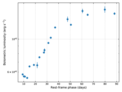
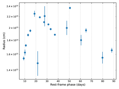
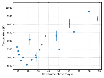
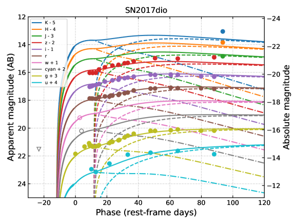
Table A1 lists the best-fitting parameters (the temperature of the photosphere , the radius of the photosphere ) of the blackbody model for the SEDs of SN 2017dio. Figures A1 and A2 present the fits of the blackbody model for SEDs of SN 2017dio and the corner plot of the 56Ni plus CSI model, respectively.
| Phase888All the phases are relative to the date of the first data which is MJD 57865.5. All epochs are transformed to the rest-frame ones. | /dof | ||
|---|---|---|---|
| (days) | (103 K) | (1015 cm) | |
| 9.06 | 38.23 | ||
| 10.15 | 10.36 | ||
| 10.97 | 78.24 | ||
| 12.97 | 26.86 | ||
| 14.96 | 73.00 | ||
| 18.75 | 13.53 | ||
| 21.61 | 0.59 | ||
| 23.51 | 131.08 | ||
| 27.37 | 17.22 | ||
| 27.86 | 0.72 | ||
| 31.23 | 127.57 | ||
| 33.26 | 129.67 | ||
| 37.03 | 176.79 | ||
| 47.72 | 0.83 | ||
| 50.59 | 737.77 | ||
| 60.57 | 0.29 | ||
| 65.02 | 82.34 | ||
| 79.80 | 0.66 | ||
| 88.13 | 66.15 |