Kernel Three Pass Regression Filter
Abstract
We forecast a single time series using a high-dimensional set of predictors. When these predictors share common underlying dynamics, an approximate latent factor model provides a powerful characterization of their co-movements Bai, (2003). These latent factors succinctly summarize the data and can also be used for prediction, alleviating the curse of dimensionality in high-dimensional prediction exercises, see Stock & Watson, (2002a). However, forecasting using these latent factors suffers from two potential drawbacks. First, not all pervasive factors among the set of predictors may be relevant, and using all of them can lead to inefficient forecasts. The second shortcoming is the assumption of linear dependence of predictors on the underlying factors. The first issue can be addressed by using some form of supervision, which leads to the omission of irrelevant information. One example is the three-pass regression filter proposed by Kelly & Pruitt, (2015). We extend their framework to cases where the form of dependence might be nonlinear by developing a new estimator, which we refer to as the Kernel Three-Pass Regression Filter (K3PRF). This alleviates the aforementioned second shortcoming. The estimator is computationally efficient and performs well empirically. The short-term performance matches or exceeds that of established models, while the long-term performance shows significant improvement.
Keywords: Forecasting, High dimension, Approximate factor model, Reproducing Kernel Hilbert space, Three-pass regression filter.
1 Introduction
In recent years, high-dimensional datasets have become increasingly accessible across various fields, including economics. It is widely acknowledged that estimation in high-dimensional settings poses a significant challenge known as the ‘curse of dimensionality’, which renders traditional finite-dimensional approaches ineffective.
Most modeling techniques applied to high-dimensional data assume the existence of a low-dimensional structure that effectively summarizes the data. One stylized feature of high-dimensional economic datasets is the presence of high and pervasive collinearity among variables, leading researchers to posit a data-generating process that assumes all variables are a function of a few latent factors. This formulation is commonly referred to as the factor model. There is a vast literature which focuses on using this latent factor structure for forecasting applications. A typical example is found in diffusion index models (Stock & Watson, (2002b)), where latent factors are derived from a high-dimensional set of variables using Principal Components Analysis (hereafter, PCA). These factors are subsequently utilized to forecast a target variable. A limitation of this PCA-based factor estimation is its unsupervised nature, i.e. that no information from the target variable is incorporated during factor estimation.
Given that the primary goal is to forecast a target rather than estimate the underlying factor structure, introducing a degree of supervision can prove beneficial. This can help in filtering out irrelevant information from the predictor set, thus enhancing the predictive accuracy .This can be done in different ways; using soft and hard thresholding methods to remove predictors with no predictive content, as in Bai & Ng, (2008), or assign varying weights to predictors based on their predictive capabilities for the target (see, for example, Huang et al., (2022)), or estimate the subset of factors that exhibit predictive power for the target rather than the complete set of factors that drive the target, as in Kelly & Pruitt, (2015).
The aforementioned models, whether utilizing PCA or supervised factor models, are predicated on the convenient assumption of linearity. However, as underscored in Goulet Coulombe et al., (2022), non-linearity often characterizes many predictive relationships, particularly over extended time horizons and within data-rich environments.
Various approaches have been proposed to integrate non-linearity into factor models. For instance, squared principal components (PCs) or principal component squared () as seen in Bai & Ng, (2008), sufficient forecasting by Fan et al., (2017), the kernel trick to estimate factors (Kutateladze, (2022)) among others. However, these approaches have limited supervision in the prediction process, if any. For example, Fan et al., (2017) estimates factors through an unsupervised method (PCA) and then derives sufficient indices using these PCs. Similarly, Kutateladze, (2022) essentially applies kernel PCA to estimate the set of factors driving a higher-dimensional space obtained by lifting the set of predictors through the kernel method. Similarly, Bai & Ng, (2008), despite employing thresholding to reduce squared PCs to a smaller set, may still encounter challenges in potentially estimating irrelevant factors within this subset, leading to inefficiency. Moreover, in Bai & Ng, (2008), a very particular form of non-linearity (quadratic) is examined, which is somewhat ad hoc.
Our paper incorporates non-linearity by introducing a novel kernel three-pass regression filter. Our approach essentially applies the three-pass filter (hereafter 3PRF) proposed by Kelly & Pruitt, (2015) to a transformed set of predictors. We adopt the lifting concept similar to Kutateladze, (2022), but instead of employing an unsupervised method like kernel PCA, we utilize a supervised method to estimate factors relevant to the target variable. The basic idea behind our approach is that many non-linear relationships observed in one space exhibit linearity in another space.
The table below summarizes our discussion by listing some popular methods in literature and how this paper is placed among them.
| Linear | Non-Linear | |
|---|---|---|
| Unsupervised | PC | kernel PCA, Sq-PC, |
| Supervised | 3PRF | This Paper |
The paper proceeds as follows. Section 2 provides a brief introduction to Kernel methods and lists examples of some widely used kernels. Section 3 introduces our estimator and discusses its similarity with the estimator of Kelly & Pruitt, (2015). We also list a set of assumptions that ensure the theoretical properties our estimators, which are given in the subsequent section 4. We present our empirical results in sections 5 and 6 and we finally conclude in section 6. Mathematical proofs and implementation details are given in the appendix.
Definitions and notations
We use to denote the vector of the target variable, i.e. . We have predictors with observations for each predictor. The cross section of predictors at a time is given by the vector . Similarly, the vector of temporal observations of a predictor is given by . We stack the predictors in a matrix , . We have proxies which we stack in a matrix , where is the -dimensional identity matrix and the -vector of ones. For matrices and of conformable dimensions, . For the transformed set of predictors , denotes the observation. Stochastic orders are denoted by the usual and . For a matrix, and denotes the element wise stochastic order, i.e., a matrix is said to be or if all it’s elements are or respectively.
2 Kernel Method
The kernel method uses an implicit mapping of the data () space into a higher-dimensional space111This higher dimensional space is Hilbert space where the inner product of the vectors is well defined. (), which contains non-linear transformations of the given data. We denote this transformation by . This transformation offers a significant advantage since many non-linear relationships can be reformulated as linear relationships in an appropriately transformed space. Transformation to a higher-dimensional space using the kernel method makes a large set of non-linear forms available, rendering the discovery of a nonlinear relationship very likely. To illustrate how a nonlinear relation can be reformulated as a linear relation with appropriately transformed variables, consider the following example. We generate 2 variables and from uniform distribution . Define a binary variable as:
It proves challenging if we attempt to use a linear boundary to separate the two classes of variable . However, upon transforming the original spaces and to and respectively, we find that the two classes can be easily distinguished as seen in figure-1.
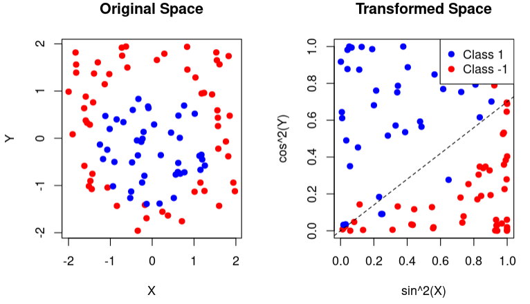
The blue points are in class 1, and the red ones are in class -1. Note that on the left-hand side, no line can achieve a decent accuracy in classification in the original space. However, we can easily do so in the transformed space on the right.
For the sake of simplicity, this example illustrates the transformation of a two-dimensional input into a two-dimensional feature space. However, the transformed space is typically high-dimensional and potentially infinite-dimensional. As the dimensions of the transformed space grow, it captures the non-linearity better by virtue of the presence of more non-linear transformations of the input data. But this high (infinite)-dimensionality of transformed space seemingly makes computations extremely challenging (infeasible). The kernel method provides a solution to this issue. Our problem necessitates the computation of the similarity measure between transformed data points and via the inner product , which appears to require knowledge of the function . The kernel function circumvents this requirement by computing the aforementioned similarity measure without necessitating knowledge of the feature map . Mercer’s condition ensures the existence of a feature map for a valid (positive definite) kernel function in Hilbert space. A detailed discussion of Mercer’s condition can be found in Appendix - A.2. In the remaining part of this section, we illustrate how the kernel function computes the inner products by showing an explicit functional form of .
Some Popular Kernel Methods and Their Working
Many popular kernel functions exist, such as polynomial, Gaussian, and sigmoid kernels. We illustrate two of them to show that kernel function can represent the products of feature map .
Polynomial Kernel
Let the functional mapping where includes a fixed term, all variables , and their respective squares and cross products. The kernel function assumes a simplified structure if we scale the linear and cross-product terms in by the constant . In other words, if we define
Then, the corresponding kernel function becomes:
This kernel can be generalized to a general degree by keeping the terms of degree at most in the expression of . This example is also discussed in Exterkate et al., (2016).
Gaussian Kernel
This kernel goes beyond the high-dimensional kernel. This kernel is, in fact, infinite-dimensional. Let and . Then, through the Taylor expansion, we can write
That is, . Kutateladze, (2022) use this kernel function in their paper which is based on kernel PCA.
3 The Estimator
We delineate the three regression passes that we use to construct our forecast. The first two passes, as explained below, are not feasible in practice, whilst the eventual closed-form solutions are. Nonetheless, these steps offer valuable insights into the underlying process of our estimator and elucidate its similarity to the well-known linear three-pass filter proposed by Kelly & Pruitt, (2015).
Below, we list the data generation process for the transformed predictor set (), the target (), and the proxies employed for supervision (). Given the data structure, it is easy to explain why this supervised methodology is effective in estimating the target relevant factors.
Assumption 1
Data generating Process.
where , and with . is the dimension of vector is the dimension of vector is the dimension of vector , and .
maps our N-dimensional predictors to a higher M-dimensional space. Assumption 1 endows this transformed set of predictors with a factor structure. An underlying factor structure among implies the existence of a low dimensional plane, projection onto which explains maximal variation in the predictors. An equivalent interpretation of a linear factor structure on would be the existence of a lower dimensional manifold which explains maximum variation in . The basis of this manifold is comprised of a few uni-dimensional orthogonal projections of .
At this juncture, it’s instructive to discuss the difference between our methodology and a set of non-linear dimension reduction methods categorized under the umbrella term ‘Sufficient Dimension Reduction (SDR)’. Sufficient dimension reduction techniques hinge upon the existence of a central subspace for , such that for every , , where is an matrix with , is a small fixed number. Matrix projects onto an L-dimensional subspace, termed the central subspace. This projection is deemed ‘sufficient’ for predicting , indicating that is redundant from the perspective of predicting . SDR accommodates non-linearity by permitting to be a non-linear function (called the link function) of , i.e. SDR posits that
In contrast, our framework posits the existence of a lower-dimensional manifold of , equivalently a subspace of 222 denotes a suitable transformation such that is ‘linearly’ independent of , conditioning on 333 is a matrix and , where the columns of constitutes an ortho-normal basis for that lower-dimensional subspace. Therefore, the projection of onto is adequate to characterize any linear dependence of on . Non-linearity, in our setup, unlike SDR, is accommodated through this projection of the transformed set of predictors444Lower dimensional subspace of the transformed set of predictors is equivalent to a non-linear manifold of the original predictors, not through a non-linear link function.
We now delineate the infeasible three-passes below.
| Stage-1 | |
|---|---|
| Pass | Description |
| 1. | Run time series regression of on for , |
| , retain slope estimate . | |
| 2. | Run cross section regression of on for , |
| , retain slope estimate . | |
| 3. | Run time series regression of on predictive factors , |
| , delivers the forecast. |
These three passes rely on the fact that the correlation between the transformed and the proxies is only due to target relevant factors. Therefore, pass 1 of the regression asymptotically yields a rotation of the relevant-factor loadings of the predictor. Cross sectional covariance between these loadings and the predictors, across , is solely affected by the target relevant factor(s). Hence, pass 2 of this process traces the factor(s) out as a slope parameter. Although these three passes offer valuable insights into the mechanics of our process, they are infeasible in practise due to the unavailability of the transformed inputs . This is where, the kernel trick shall prove to be handy. To see this, we note that factor(s), their predictive coefficients and the forecast can be expressed in closed form as below,
The estimated factor(s) :
The estimated coefficient(s) of the factor(s) :
Finally, the estimated target :
These are obtained by simply replacing by in the three-pass regression filter of Kelly & Pruitt, (2015). As evident from the expression of , our three-pass filter applied on the transformed predictor space results in a favorable scenario where the eventual estimate of the factor(s) depends upon the transformed predictors only through their dot products in the transformed space. This holds true for and as well.
This inner product can be computed using a suitable kernel function. Alternatively, it can be inferred that employing a positive semidefinite (psd) kernel function to calculate dot products in these derived expressions is akin to executing the three-pass filter process on the implied transformed space, which, according to Mercer’s theorem, is guaranteed to exist.
The Kernel three-pass regression, just like the linear 3PRF, relies on the availability of suitable proxies. Kelly & Pruitt, (2015) shows that such proxies can always be constructed using the target variable . That process is explained below.
| 0. | Initialize . For . (L is the total number of proxies) |
|---|---|
| 1. | Define the automatic proxy to be . Stop if ; otherwise proceed. |
| 2. | Compute the k3PRF for target using cross-section using statistical proxies 1 through . |
| Denote the resulting forecast . | |
| 3. | Calculate , advance , and go to step 1. |
Assumption 1 lays out the factor structure of our model. Below, we delineate a set of additional assumptions under which our model delivers consistent forecasts.
Assumption 2
(Factors, Loadings and Residuals).
Let . For any and some ,
-
1.
.
-
2.
,, .
-
3.
-
4.
and
-
5.
, and is independent of and for any .
Assumption 2.1 requires that our factors are regular in the sense that their covariance matrix is well-behaved asymptotically. Assumption 2.2 is an adaptation from Kelly & Pruitt, (2015). Since we assume a factor structure on the transformed space instead of the original predictor space, the normalization in various terms features and not , where is the dimension of our transformed space. Assumptions 2.3-2.5 borrowed from Kelly & Pruitt, (2015), impose regularity on various error processes.
Assumption 3
(Dependence).
Let denote the element of . For and any
-
1.
and , and
a. b.
c. d. -
2.
-
3.
-
4.
.
-
5.
-
6.
.
-
7.
Assumption 3.1-3.2 allow various forms of weak cross-sectional and temporal dependence between the idiosyncratic components of the transformed predictors. These assumptions characterize our ‘Approximate’ factor model. The terminology of approximate, as opposed to a strict factor model, alludes to the allowance of these weak correlations, as outlined by Chamberlain & Rothschild, (1983). These assumptions are standard in the literature; see Bai, (2003). Assumption 3.4-3.7 are either borrowed from or are weaker versions of Assumptions in Kelly & Pruitt, (2015). They are reasonable because each of them involves a product of orthogonal series.
Assumption 4
(Normalization).
-
1.
-
2.
is diagonal, positive definite, and each diagonal element is unique and bounded.
Assumption 4 is a normalization assumption that is common in factor model literature. It pertains to the non-identifiability of the true factor(s). It is well known that only the vector space spanned by the factor(s) can be consistently estimated but not the factor themselves. Imposing some normalization condition for the uniqueness of solution(s) is common in literature.
Assumption 5
(Relevant Proxies).
-
1.
-
2.
is non-singular.
5 outlines the utility of using proxies. Proxies are target-relevant in the sense that they only load on the factor(s) which have any explanatory power for the target. Non-singularity of ensures that none of the proxies are redundant.
4 Results
Define . Define where, and
This theorem establishes the estimated factor(s) convergence to the true factors up to a rotation. It is well known in the literature on factor models555This feature of inherent unidentifiability has been emphasized in Bai, (2003), Kelly & Pruitt, (2015) among other papers. The normalization imposed in assumption 5 is done to handle this issue., that true underlying factor(s) are not identifiable; we instead estimate a rotated version of the true factors, which preserves their span.
Define , where
and
This theorem establishes the convergence of the predictive coefficients to a rotation of the true coefficients. Just like in the case of factor(s), true coefficients are not identifiable and we instead estimate their rotation. The rates established in Theorems 1 and 2 differ from the rates established in Kelly & Pruitt, (2015) and the reason is that our definition of rotation matrices and are different from Kelly & Pruitt, (2015). (See Remark 1).
Remark 1
As highlighted in Bai & Ng, (2006) and also emphasized in Kelly & Pruitt, (2015), the presence of matrices and in Theorem 1 and 2 highlight the fact we are essentially estimating a vector space. These theorems “pertain to the difference between and the space spanned by ”. The product equals an identity matrix, cancelling the rotations in the estimated coefficients and the factors; thereby consistently estimating direction spanned by . However, this characteristic is absent in Theorems 5 and 6 of Kelly & Pruitt, (2015). The matrices and as defined in their paper do not necessarily yield a product that equals an identity matrix.
Combining Theorem 1 and 2, the convergence of follows directly. Our proof, unlike Kelly & Pruitt, (2015) uses the convergence results for the estimated factor(s) and coefficients to obtain this result.
Remark 2
The rates established in Theorem 1, 2 and 3 are different from the result in Kelly & Pruitt, (2015) where the corresponding rates are , and 666For our case, it should have been as per their theorem since we apply 3PRF to the transformed M-dimesnional space. respectively (see Theorems 4, 5 and 6 in their paper). For Theorem 1 and 2, the difference is explained by a different definition of the rotation matrices in our paper (see Remark 1). For establishing the convergence of , their proof follows two steps. First they show that , where is defined in their appendix. Then then they argue that . Since 777The definition of and fact that it is can be seen from the proof of Theorem 6 of Kelly & Pruitt, (2015) is , would diverge to infinity and their statement would be false. We presume that they erroneously wrote this and instead wanted to imply that . However this statement is false because has random elements which converge to 0 at a rate which is
5 Empirical Applications
In this section, we apply our proposed method to real-world applications, focusing on forecasting time series variables across various economic domains such as macroeconomics, finance, labor, housing, and prices. To assess the performance of our approach, we conduct comparative analyses against competitive methods, employing the out-of-sample performance metric as a benchmark. Additionally, we provide detailed explanations of our data, including the transformations applied to ensure stationarity and the optimization of hyperparameters related to kernel functions.
We compare our method against six different forecasting methods. The first is the PCA-based factor model proposed by Stock & Watson, (2002b); we write it as PCA in our performance tables. Following on PCA-based methods, we compare against PC-Squared (PC-Sq) and Squared-PC(Sq-PC) of Bai & Ng, (2008). The fourth method is the kernel-based PCA (kPCA) method implemented in Kutateladze, (2022). The fifth is our linear counterpart, the 3PRF. The last is an autoregressive model of lag order two. Some of these methods require tuning of hyper-parameters to provide the best results, we do tune them as discussed in the subsection-5.2. Further, kernel method-based papers report results with different kernels; however, we only report the results with a Gaussian kernel to save some space.
5.1 Performance Metric: Out of Sample
We employ out-of-sample relative to the historical mean as our performance metric to assess various forecasting methods alongside our own. Out-of-sample indicates goodness of fit on unseen data, providing insights into the predictive accuracy of a model. Mathematically, out-of-sample is computed as follows:
Here, the numerator quantifies the squared deviation between the model’s predictions and the true values in the test data. At the same time, the denominator measures the deviation of the true values from the historical mean in the test data. It is important to note that we utilize the mean of the training data for the historical mean, as in real-world forecasting scenarios, access to the training mean is typically available.
It is noteworthy that out-of-sample ranges from to , unlike in-sample , which ranges from zero to one. A positive out-of-sample indicates that the forecasting method outperforms the historical average. At the same time, a negative value suggests that the forecasting method performs worse than a simple method that forecasts equal to the historical average.
We adopt the rolling window method to compute out-of-sample , consistent with standard practices in the literature. Appendix B.1 provides a detailed exposition of our methodology.
5.2 Data and Hyper-Parameter Tuning
We utilize the quarterly macroeconomic dataset, FRED-QD. It covers the time span of 1959-2023. This dataset encompasses a comprehensive array of variables exceeding 250, including macroeconomic (such as GDP, Consumption, and Investment), financial, labor market, housing, and industrial and manufacturing variables. Our forecasting endeavors focus on a single target time series while leveraging the remaining variables within the predictor set. Our main text shows the forecasting of important variables from various domains, such as macro, labor, housing, finance, prices, etc. For ease of reference, we present a tabulation comprising the mnemonic codes and details of the variables in the FRED-QD dataset alongside their counterparts in the Stock-Watson dataset in Appendix B.2.
5.2.1 Data Transformation
PCA encounters challenges when applied to nonstationary time series commonly found in economics and finance. Nonstationary variables lack a defined population mean, and the sample standard deviation tends to diverge as the number of observations increases. Onatski & Wang, (2021) discusses some of the significant issues arising from applying PCA to nonstationary data in detail. Generally, researchers address this by manually examining each series to identify necessary transformations before computing principal components. Hamilton & Xi, (2024) offers an improved method of transformation to achieve the stationarity of the predictor set. We use their method to remove nonstationarity from our data.
Scholars in the literature often employ sample periods devoid of structural breaks; for instance, Fan et al., (2023) says “There exist significant structural breaks for many variables around the year of financial crisis in 2008 which makes our data non-stationary even after performing the suggested transformations”. Therefore, our study focuses on the stationary period spanning from 1965 to 2007888Another indirect advantage of the choice of this sample period is that it gives us the number of samples less than the number of predictors (), hence a truly high-dimensional scenario to test our method in.. For the sanity check, we conduct analyses on different combinations of the sample periods, including the entire available sample period from 1959 to 2023, and find no qualitative discrepancies in our findings.
In our main analysis, the sample period from 1964:Q4 to 2007:Q1 comprises observations (periods) and variables (predictors). While the data is initially available for around 250 series, those with missing values are removed; this leaves us with a total of 176 series. We adopt the rolling window methodology for model training and hyper-parameter tuning, utilizing 70% of the total observations as the width of the rolling window. We observe qualitatively similar performance across varying window sizes (50%, 60% of total data). Subsequently, we evaluate the forecasting performance on out-of-sample data and present the results in the tables.
5.2.2 Hyper-parameter Tuning
Our methodology incorporates the kernel as a fundamental element of the estimation process. However, the kernel function includes a hyperparameter that necessitates optimization. Concurrently, a similar hyperparameter requires tuning in the context of a competitor method, namely kernel PCA. Thus, we employ an identical tuning procedure for both methodologies. We adopt a Gaussian kernel, which relies on a single hyperparameter, denoted as , for our specific applications. Due to the nature of our dataset, which comprises time series data, conventional methods such as random sampling for k-fold cross-validation are not directly applicable. Instead, we partition the data into two folds and conduct cross-validation to determine the optimal tuning parameter. Further elaboration on the algorithm employed for this purpose is provided in the appendix-B.3.
Furthermore, among our competitive methodologies, certain approaches are based on PCA, necessitating the judicious selection of the number of principal components to be included in the analysis. To address this, we employ the eigenvalue ratio test method proposed by Ahn & Horenstein, (2013). This method computes the ratio of each eigenvalue to its predecessor and selects the number of principal components corresponding to the index where this ratio attains its maximum value.
5.3 Forecasting Using Theory Guided Proxies
We show the utility of theory-guided proxies as in Kelly & Pruitt, (2015) to predict certain variables. In this section, we present a comparison with the linear benchmark, i.e., 3PRF.
The primary strength of our methodology lies in its ability to accurately forecast over longer horizons, where non-linear relationships become more pronounced. However, for the purposes of this section, we restrict our analysis to one-period ahead forecasting. Our results show that our approach outperforms its closest competitor even in the short term. It is essential to note that the primary objective of this subsection is to establish the viability of theory-guided proxies rather than to conduct a comprehensive comparison with competing methods. A more extensive performance evaluation will be presented in subsequent subsections, where we used the auto-proxy method discussed in table-3 to construct forecasts using Kernel 3PRF.
5.3.1 National Income Identity
Sometimes, the context of the problem gives us good choices for proxy variables. There is ample evidence that consumption and investments can be reasonable proxies for a country’s gross domestic product (GDP). The two proxies affect the GDP through the multiplier effect. Therefore, for the GDP (Y), we can choose consumption (C) and Investment (I) as proxy variables. We forecast GDP by taking combinations of consumption and investment as proxies. The results are presented in Table-4.
| Proxy | 3PRF | k3PRF |
|---|---|---|
| Consumption and Investment | 0.621 | 0.768 |
| Investment | 0.627 | 0.748 |
| Consumption | 0.589 | 0.760 |
It is clear that using the proxies works, and our method performs better than the nearest competitive method Kelly & Pruitt, (2015).
5.3.2 Quantity Theory of Money
In another application of theory-guided proxies, we utilize the quantity theory of money to forecast inflation using GDP and money supply as proxies. The quantity theory of money equation states:
Our objective is to forecast inflation. In our dataset, represents the change in GDP, while signifies the changes in money supply using log growth in M1. Similar to Fama (1981), changes in velocity, which are challenging to quantify, serve as the error term in the forecasting relationship. The timing is aligned such that proxies observed at time are utilized to extract information from the predictors at time for forecasting inflation at time . The results for one-period ahead inflation forecasts are presented in Table-5.
| Proxy | 3PRF | k3PRF |
|---|---|---|
| GDP and Money Supply | 0.265 | 0.265 |
| GDP | 0.037 | 0.037 |
| Money Supply | 0.350 | 0.355 |
The results indicate that the theory-guided proxies effectively capture inflation dynamics, yielding performance comparable to the closest competitor. It is important to emphasize again that this analysis focuses on one-step-ahead forecasts, which are not the primary strength of our methodology. The purpose of presenting these results is solely to demonstrate the efficacy of the proxies.
5.4 Long and Short-Run Forecasting: Comparative Performance Plots
Linear equations may approximate the relationships between targets and predictors effectively when the analysis time span is sufficiently short. However, as the time span expands, incorporating non-linearities becomes crucial, as noted by Goulet Coulombe et al., (2022). Linear methods exhibit deteriorating performance as the forecasting horizon extends into the future. Thus, the primary strength of our methodology lies in addressing longer-horizon forecasting challenges. Nevertheless, we demonstrate that even in shorter-horizon forecasting scenarios, our approach distinctly outperforms the nearest competitor Kelly & Pruitt, (2015). In the subsequent section, we present comparative plots, reserving detailed and comprehensive comparisons for subsequent sub-sections.
5.4.1 Short Horizon Forecasting
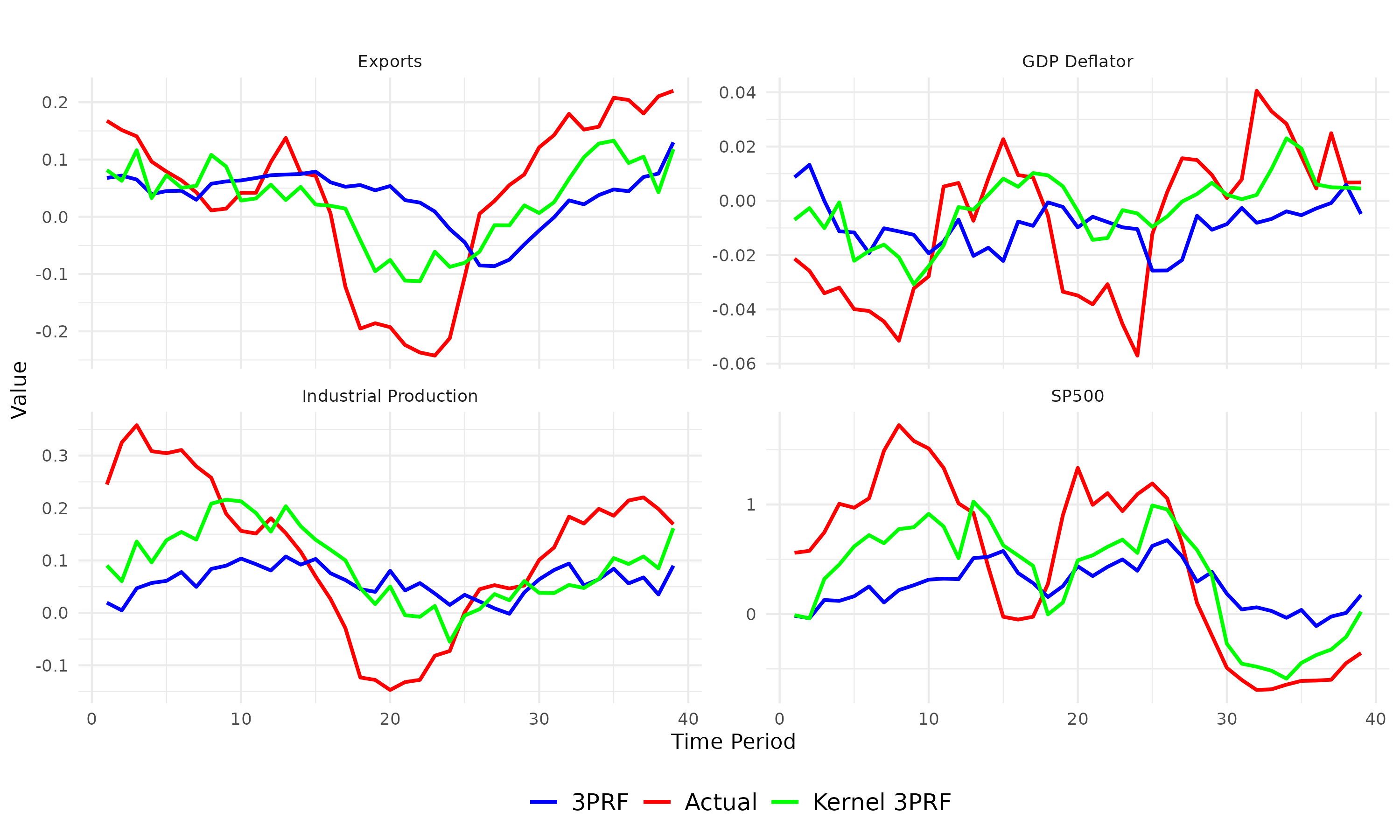
While kernel functions are recognized for their ability to effectively capture non-linear relationships between variables, it’s essential to acknowledge that linear relationships can also be effectively modeled by kernel functions by selecting an appropriate tuning hyperparameter.
In this sub-section, we aim to demonstrate the superiority of our kernel-based forecasting method over the closest linear forecasting method (3PRF) in the one-step-ahead forecasting problem. We present the one-step-ahead forecasted series using our method (k3PRF) and 3PRF alongside the true values of the target variables in figure-3. Specifically, we compare the performance across four different types of economic series from different domains: macro series Exports, price series GDP Deflator, manufacturing series Industrial Production, and financial series the S&P 500 Index.

The plots in figure-3 clearly illustrate that our predictions closely align with the true series, surpassing the predictions generated by 3PRF. Our method captures significant fluctuations, including notable drops and peaks, demonstrating its efficacy in short-term forecasting scenarios.
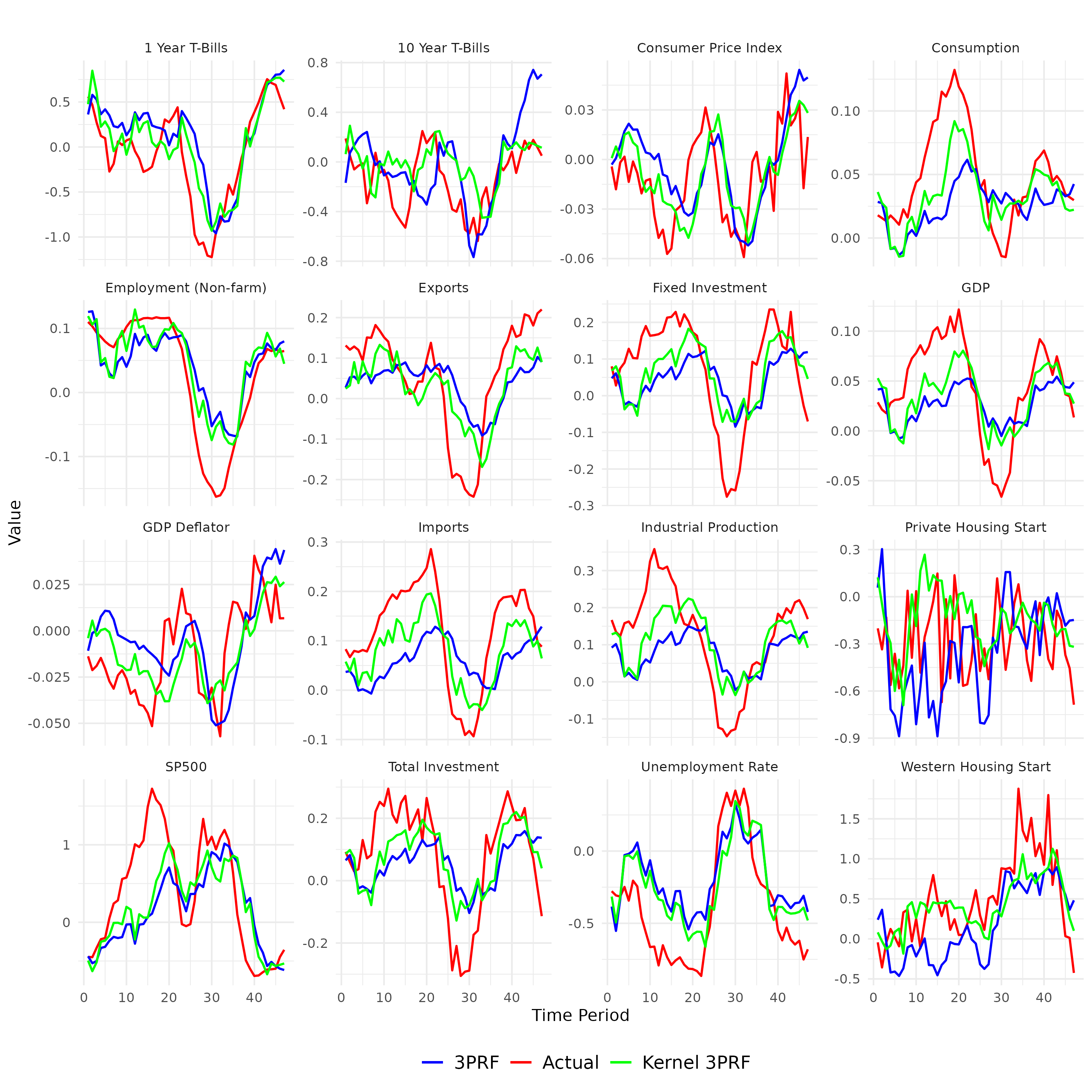
5.4.2 Long Horizon Forecasting
In this section, we plot the long-horizon (twelve periods ahead) forecasts generated by the 3PRF method and our method against the actual value of the target series in figure-4. We compare the two methods on the same four economic series as in the previous subsection.
We observe that the long-horizon forecasts of our competitor, the 3PRF method, tend to flatter, i.e., approaching a historical mean. Whereas our method can accurately track the true series by capturing ups and downs. Although it is acknowledged that absolute predictability may diminish over longer horizons relative to linear methods, our approach continues to demonstrate robust performance, even on extended forecasting horizons.
5.5 Forecasting Macroeconomic Variables
An astute economic decision, such as monetary policy formulation, hinges upon well-informed anticipations of future trends in macroeconomic and financial data. Consequently, forecasting macroeconomic variables emerges as a pivotal pursuit for economists. Quoting Federal Reserve of New York’s website, Kim & Swanson, (2014) notes, “In formulating the nation’s monetary policy, the Federal Reserve considers a number of factors, including the economic and financial indicators which follow, as well as the anecdotal reports compiled in the Beige Book. Real Gross Domestic Product (GDP); Consumer Price Index (CPI); Nonfarm Payroll Employment Housing Starts; Industrial Production/Capacity Utilization; Retail Sales; Business Sales and Inventories; Advance Durable Goods Shipments, New Orders and Unfilled Orders; Lightweight Vehicle Sales; Yield on 10-year Treasury Bond; S&P 500 Stock Index; M2”. We, therefore, aim to forecast some of these crucial indicators in this paper. We compare the performance of our model against the competitors. This section forecasts seven macro series: GDP, Consumption, Investment, Exports, Imports, Fixed Investment, and Industrial Production (Final).
| GDP | |||||||||
|---|---|---|---|---|---|---|---|---|---|
| Method | h=1 | h=2 | h=3 | h=4 | h=6 | h=8 | h=10 | h=12 | |
| AR(2) | 0.929 | 0.906 | 0.843 | 0.719 | 0.302 | -0.216 | -0.555 | -0.724 | |
| PCA | 0.717 | 0.650 | 0.575 | 0.492 | 0.311 | 0.130 | -0.001 | -0.075 | |
| Sq-PC | 0.615 | 0.593 | 0.552 | 0.488 | 0.290 | 0.076 | -0.092 | -0.166 | |
| PC-Sq | 0.773 | 0.733 | 0.676 | 0.594 | 0.398 | 0.175 | 0.008 | -0.063 | |
| kPCA | 0.638 | 0.589 | 0.528 | 0.464 | 0.322 | 0.204 | 0.060 | 0.063 | |
| 3PRF | 0.667 | 0.619 | 0.561 | 0.493 | 0.341 | 0.193 | 0.130 | 0.201 | |
| k3PRF | 0.808 | 0.788 | 0.757 | 0.701 | 0.603 | 0.544 | 0.608 | 0.434 | |
| Consumption | |||||||||
| Method | h=1 | h=2 | h=3 | h=4 | h=6 | h=8 | h=10 | h=12 | |
| AR(2) | 0.957 | 0.943 | 0.892 | 0.805 | 0.485 | 0.015 | -0.375 | -0.557 | |
| PCA | 0.573 | 0.554 | 0.504 | 0.430 | 0.238 | 0.038 | -0.093 | -0.155 | |
| Sq-PC | 0.546 | 0.541 | 0.499 | 0.428 | 0.235 | 0.025 | -0.137 | -0.206 | |
| PC-Sq | 0.611 | 0.637 | 0.628 | 0.596 | 0.412 | 0.161 | -0.041 | -0.128 | |
| kPCA | 0.433 | 0.419 | 0.369 | 0.319 | 0.143 | 0.076 | 0.039 | 0.181 | |
| 3PRF | 0.589 | 0.547 | 0.501 | 0.464 | 0.386 | 0.196 | 0.169 | 0.326 | |
| k3PRF | 0.713 | 0.730 | 0.720 | 0.741 | 0.770 | 0.747 | 0.275 | 0.496 | |
| Investment | |||||||||
| Method | h=1 | h=2 | h=3 | h=4 | h=6 | h=8 | h=10 | h=12 | |
| AR(2) | 0.830 | 0.807 | 0.711 | 0.546 | 0.087 | -0.450 | -0.544 | -0.586 | |
| PCA | 0.516 | 0.393 | 0.300 | 0.231 | 0.149 | 0.089 | 0.030 | 0.011 | |
| Sq-PC | 0.398 | 0.348 | 0.297 | 0.238 | 0.099 | -0.022 | -0.083 | -0.065 | |
| PC-Sq | 0.605 | 0.488 | 0.391 | 0.296 | 0.186 | 0.090 | 0.017 | 0.044 | |
| kPCA | 0.479 | 0.390 | 0.317 | 0.272 | 0.196 | 0.030 | -0.016 | -0.013 | |
| 3PRF | 0.597 | 0.484 | 0.429 | 0.369 | 0.273 | 0.111 | 0.083 | 0.176 | |
| k3PRF | 0.760 | 0.640 | 0.478 | 0.605 | 0.433 | 0.199 | 0.169 | 0.389 |
| Exports | |||||||||
|---|---|---|---|---|---|---|---|---|---|
| Method | h=1 | h=2 | h=3 | h=4 | h=6 | h=8 | h=10 | h=12 | |
| AR(2) | 0.928 | 0.926 | 0.906 | 0.863 | 0.723 | 0.522 | 0.409 | 0.302 | |
| PCA | 0.353 | 0.306 | 0.248 | 0.193 | 0.123 | 0.107 | 0.106 | 0.109 | |
| Sq-PC | 0.275 | 0.249 | 0.215 | 0.183 | 0.120 | 0.056 | 0.008 | -0.013 | |
| PC-Sq | 0.399 | 0.326 | 0.243 | 0.166 | 0.073 | 0.066 | 0.113 | 0.194 | |
| kPCA | 0.027 | 0.033 | 0.033 | 0.270 | 0.142 | -0.002 | -0.044 | 0.130 | |
| 3PRF | 0.535 | 0.523 | 0.459 | 0.389 | 0.223 | 0.137 | 0.109 | 0.092 | |
| k3PRF | 0.724 | 0.705 | 0.641 | 0.602 | 0.546 | 0.575 | 0.600 | 0.631 | |
| Imports | |||||||||
| Method | h=1 | h=2 | h=3 | h=4 | h=6 | h=8 | h=10 | h=12 | |
| AR(2) | 0.969 | 0.964 | 0.951 | 0.931 | 0.845 | 0.710 | 0.577 | 0.460 | |
| PCA | 0.417 | 0.380 | 0.343 | 0.306 | 0.233 | 0.154 | 0.072 | 0.006 | |
| Sq-PC | 0.395 | 0.373 | 0.341 | 0.299 | 0.194 | 0.079 | -0.005 | -0.046 | |
| PC-Sq | 0.477 | 0.462 | 0.438 | 0.398 | 0.306 | 0.182 | 0.060 | 0.000 | |
| kPCA | 0.421 | 0.389 | 0.348 | 0.311 | 0.241 | 0.081 | 0.064 | 0.033 | |
| 3PRF | 0.546 | 0.506 | 0.468 | 0.436 | 0.394 | 0.347 | 0.322 | 0.338 | |
| k3PRF | 0.777 | 0.783 | 0.790 | 0.786 | 0.749 | 0.411 | 0.388 | 0.558 | |
| Fixed Invest. | |||||||||
| Method | h=1 | h=2 | h=3 | h=4 | h=6 | h=8 | h=10 | h=12 | |
| AR(2) | 0.905 | 0.881 | 0.818 | 0.682 | 0.224 | -0.267 | -0.467 | -0.605 | |
| PCA | 0.490 | 0.384 | 0.290 | 0.220 | 0.134 | 0.088 | 0.042 | 0.016 | |
| Sq-PC | 0.401 | 0.352 | 0.293 | 0.231 | 0.095 | -0.024 | -0.077 | -0.064 | |
| PC-Sq | 0.595 | 0.492 | 0.385 | 0.314 | 0.208 | 0.104 | 0.030 | 0.068 | |
| kPCA | 0.498 | 0.407 | 0.315 | 0.250 | 0.167 | 0.039 | -0.034 | 0.007 | |
| 3PRF | 0.525 | 0.454 | 0.389 | 0.348 | 0.251 | 0.122 | 0.127 | 0.226 | |
| k3PRF | 0.736 | 0.659 | 0.426 | 0.578 | 0.265 | 0.235 | 0.261 | 0.359 | |
| IP : Final | |||||||||
| Method | h=1 | h=2 | h=3 | h=4 | h=6 | h=8 | h=10 | h=12 | |
| AR(2) | 0.830 | 0.807 | 0.711 | 0.546 | 0.087 | -0.450 | -0.544 | -0.586 | |
| PCA | 0.516 | 0.393 | 0.300 | 0.231 | 0.149 | 0.089 | 0.030 | 0.011 | |
| Sq-PC | 0.398 | 0.348 | 0.297 | 0.238 | 0.099 | -0.022 | -0.083 | -0.065 | |
| PC-Sq | 0.605 | 0.488 | 0.391 | 0.296 | 0.186 | 0.090 | 0.017 | 0.044 | |
| kPCA | 0.479 | 0.390 | 0.317 | 0.272 | 0.196 | 0.030 | -0.016 | -0.013 | |
| 3PRF | 0.597 | 0.484 | 0.429 | 0.369 | 0.273 | 0.111 | 0.083 | 0.176 | |
| k3PRF | 0.760 | 0.640 | 0.478 | 0.605 | 0.433 | 0.199 | 0.169 | 0.389 |
Results and Disucssion
To present the results in a tidy manner, we make two tables. In table-6, we present the forecasting performance on three series: GDP, Consumption, and Investment. To keep track of the presentation, we informally call it ‘Group-I’.
Table-7 shows comparative forecasting performance on ‘Group-II’ macro variables: Exports, Imports, Fixed Investments, and Industrial Production (Final Index). Further detail on these variable series is available in appendix-B.2.
The numbers reported in the table are out of sample defined earlier in the text. We present performance for various forecast horizons ranging from one period ahead to twelve periods ahead.
An empirical observation highlights that among various unsupervised forecasting methodologies, including PCA, Squared-PC, PC-squared, and non-linear unsupervised approaches such as kernel PCA, none exhibit superior performance compared to our proposed method across any forecast horizon for the seven series under consideration. While the supervised linear forecasting model 3PRF demonstrates improved performance relative to the unsupervised techniques, it still falls short of outperforming our non-linear supervised approach. Notably, the autoregressive (AR) model emerges as the sole contender capable of surpassing our method in the short term. Remarkably, our approach exhibits only a marginal performance differential compared to the AR model in shorter forecast horizons yet significantly outperforms it over longer forecast horizons.
In summary, the consistent empirical observation across all series suggests that our method progressively outperforms all alternative methodologies with increasing forecast horizons. Notably, the AR model remains a competitive rival in the short term, attributed to the linear model’s relative advantage in capturing short-term dynamics where nonlinearities may not yet manifest. Consequently, our method emerges as a dependable and preferred forecasting framework across all forecast horizons in macroeconomic prediction tasks.
5.6 Forecasting Labor Market Variables
The examination of the unemployment rate and total non-farm employment offers a deeper understanding of the labor market dynamics within an economy. The labor market is a pivotal element given its centrality in providing income and livelihoods for most economic actors. Consequently, fluctuations in the labor market exert profound impacts on consumer spending patterns and inflationary pressures. These indicators serve as crucial inputs into important economic decisions, notably informing the formulation of both fiscal and monetary policies to achieve goals. We forecast these two series and present the results in table-8.
| Employment | |||||||||
|---|---|---|---|---|---|---|---|---|---|
| Method | h=1 | h=2 | h=3 | h=4 | h=6 | h=8 | h=10 | h=12 | |
| AR(2) | 0.992 | 0.961 | 0.864 | 0.693 | 0.170 | -0.429 | -0.881 | -1.079 | |
| PCA | 0.786 | 0.728 | 0.604 | 0.435 | 0.057 | -0.219 | -0.258 | -0.146 | |
| Sq-PC | 0.528 | 0.498 | 0.440 | 0.361 | 0.167 | -0.024 | -0.109 | -0.098 | |
| PC-Sq | 0.836 | 0.795 | 0.679 | 0.510 | 0.131 | -0.139 | -0.210 | -0.110 | |
| kPCA | 0.832 | 0.790 | 0.702 | 0.587 | 0.370 | 0.196 | 0.112 | 0.059 | |
| 3PRF | 0.765 | 0.731 | 0.712 | 0.662 | 0.407 | 0.312 | 0.264 | 0.229 | |
| k3PRF | 0.929 | 0.895 | 0.846 | 0.768 | 0.556 | 0.444 | 0.441 | 0.584 | |
| Unemp Rate | |||||||||
| Method | h=1 | h=2 | h=3 | h=4 | h=6 | h=8 | h=10 | h=12 | |
| AR(2) | 0.963 | 0.927 | 0.847 | 0.721 | 0.378 | 0.011 | -0.150 | -0.196 | |
| PCA | 0.810 | 0.853 | 0.849 | 0.809 | 0.648 | 0.426 | 0.255 | 0.133 | |
| Sq-PC | 0.825 | 0.852 | 0.849 | 0.821 | 0.686 | 0.457 | 0.251 | 0.097 | |
| PC-Sq | 0.798 | 0.849 | 0.851 | 0.820 | 0.687 | 0.497 | 0.304 | 0.225 | |
| kPCA | 0.610 | 0.664 | 0.672 | 0.675 | 0.647 | 0.562 | 0.440 | -0.035 | |
| 3PRF | 0.913 | 0.914 | 0.863 | 0.802 | 0.638 | 0.475 | 0.402 | 0.471 | |
| k3PRF | 0.924 | 0.937 | 0.903 | 0.846 | 0.674 | 0.508 | 0.459 | 0.390 |
Result and Discussions
We present the results in table-8. It’s worth noting that the overall trends in the total non-farm employment series align with our macroeconomic time series discussion. Importantly, our method consistently outperforms competitors in longer horizon forecasting (), a testament to its robustness and reliability. As we extend the forecast horizons, the margin of our method’s superior performance continues to grow, instilling confidence in its effectiveness. In the short term, our method may not outperform the autoregressive model, but it still ranks second and is only slightly behind. Similarly, in forecasting the unemployment rate, our method consistently outperforms all other methods, including the autoregressive (AR) model, from onwards.
To summarize, our findings mirror those of the macroeconomic series forecasting. Our method consistently demonstrates superior performance across various forecast horizons and labor market indicators, reaffirming its reliability and preference in macroeconomic prediction tasks.
5.7 Forecasting Housing Variables
The housing market is characterized by its multidimensional aspect, involving various natures and functions. Houses serve as places of residence and vehicles for wealth accumulation, asset transfer to the next generation, and investment. Also, housing comprises a significant portion of household assets, making it an important factor in household decision-making. Consequently, distortions in the housing market can affect household spending and the broader economy through institutions such as mortgage banks. Therefore, forecasting housing market activities holds substantial value. In this section, we forecast two housing series: the first is Privately Owned Housing Starts (HStart), and the second is Privately Owned Housing Starts in the Western Census region(HStart-W).
| HStart | |||||||||
|---|---|---|---|---|---|---|---|---|---|
| Method | h=1 | h=2 | h=3 | h=4 | h=6 | h=8 | h=10 | h=12 | |
| AR(2) | 0.048 | -0.029 | -0.140 | -0.216 | -0.380 | -0.157 | -0.131 | -0.105 | |
| PCA | -1.360 | -0.799 | -0.317 | -0.052 | 0.172 | 0.259 | 0.086 | 0.085 | |
| Sq-PC | -1.226 | -0.688 | -0.196 | 0.095 | 0.314 | 0.453 | 0.183 | 0.100 | |
| PC-Sq | -1.473 | -0.936 | -0.371 | -0.004 | 0.278 | 0.188 | -0.176 | -0.024 | |
| kPCA | -0.199 | -0.074 | -0.157 | 0.244 | 0.408 | -0.101 | -0.325 | 0.101 | |
| 3PRF | 0.092 | 0.272 | 0.064 | -0.223 | -0.391 | -0.205 | -0.220 | -0.653 | |
| k3PRF | 0.138 | 0.204 | 0.231 | 0.245 | 0.230 | 0.253 | 0.116 | 0.073 | |
| HStart-W | |||||||||
| Method | h=1 | h=2 | h=3 | h=4 | h=6 | h=8 | h=10 | h=12 | |
| AR(2) | 0.571 | 0.540 | 0.495 | 0.386 | 0.003 | -0.397 | -0.402 | -0.787 | |
| PCA | 0.326 | 0.433 | 0.481 | 0.516 | 0.405 | 0.169 | -0.070 | -0.182 | |
| Sq-PC | 0.201 | 0.318 | 0.356 | 0.372 | 0.184 | -0.053 | -0.248 | -0.323 | |
| PC-Sq | 0.359 | 0.402 | 0.414 | 0.459 | 0.310 | 0.033 | -0.135 | -0.244 | |
| kPCA | 0.287 | 0.336 | 0.379 | 0.442 | 0.447 | -0.135 | -0.147 | -0.062 | |
| 3PRF | 0.571 | 0.475 | 0.231 | 0.084 | -0.031 | 0.094 | 0.260 | 0.253 | |
| k3PRF | 0.586 | 0.464 | 0.207 | 0.554 | 0.178 | 0.141 | 0.160 | 0.463 |
Results and Discussions–
Table-9 presents the forecasting results. One can note that predicting the privately owned housing start time series is very difficult. While most forecasting methods cannot beat the historical average, our method performs better than all other methods at all horizons. On the other hand, while it is relatively easy to forecast housing in the western census region, our method performs better than all other methods except for one or two cases. The results in other housing variables follow similar patterns; therefore, we omit them for the simplicity of exposition.
Therefore, it is clear that our method holds value in a difficult forecasting problem in both the short and long run. We also enjoy a better method for long-run forecasting problems in the housing market series.
5.8 Forecasting Price Variables
Inflation, a topic of significant interest in the market, media, and academia, holds a crucial role due to its impact on the common consumers. Particularly, inflation adversely affects low-wage earners, underscoring its societal implications. The relevance of our research is underscored by the fact that one of the primary objectives of the Federal Reserve or Central Bank is to control inflation. In this context, we focus on forecasting two key price time series: the GDP Deflator and the Consumer Price Index (CPI), which are pivotal in understanding and predicting inflation. The motivation behind choosing these two price series is that– on the one hand, the GDP Deflator considers the macroeconomic picture at the aggregate level. At the same time, the CPI measure informs us of the inflation faced by the consumer at a disaggregated level.
| GDP Deflator | |||||||||
|---|---|---|---|---|---|---|---|---|---|
| Method | h=1 | h=2 | h=3 | h=4 | h=6 | h=8 | h=10 | h=12 | |
| AR(2) | 0.797 | 0.774 | 0.740 | 0.657 | 0.418 | 0.146 | 0.156 | 0.077 | |
| PCA | 0.444 | 0.276 | 0.056 | -0.184 | -0.408 | -0.347 | -0.221 | -0.057 | |
| Sq-PC | 0.299 | 0.145 | -0.035 | -0.168 | -0.245 | -0.230 | -0.192 | -0.108 | |
| PC-Sq | 0.431 | 0.268 | 0.104 | -0.039 | -0.106 | -0.038 | -0.111 | -0.182 | |
| kPCA | -0.032 | 0.247 | -0.021 | 0.008 | 0.003 | 0.004 | 0.029 | -0.023 | |
| 3PRF | 0.584 | 0.496 | 0.426 | 0.243 | 0.174 | 0.279 | 0.300 | 0.155 | |
| k3PRF | 0.667 | 0.632 | 0.563 | 0.476 | 0.479 | 0.413 | 0.197 | 0.512 | |
| CPI | |||||||||
| Method | h=1 | h=2 | h=3 | h=4 | h=6 | h=8 | h=10 | h=12 | |
| AR(2) | 0.704 | 0.706 | 0.620 | 0.565 | 0.397 | 0.211 | 0.062 | -0.038 | |
| PCA | 0.660 | 0.535 | 0.364 | 0.154 | -0.163 | -0.252 | -0.248 | -0.173 | |
| Sq-PC | 0.410 | 0.296 | 0.161 | 0.049 | -0.055 | -0.156 | -0.200 | -0.173 | |
| PC-Sq | 0.649 | 0.512 | 0.353 | 0.186 | -0.019 | -0.087 | -0.187 | -0.228 | |
| kPCA | 0.440 | 0.380 | -0.050 | 0.189 | -0.043 | -0.024 | 0.042 | -0.006 | |
| 3PRF | 0.641 | 0.566 | 0.487 | 0.352 | 0.192 | 0.241 | 0.255 | 0.141 | |
| k3PRF | 0.676 | 0.612 | 0.541 | 0.463 | 0.469 | 0.434 | 0.349 | 0.477 |
Results and Discussion
Table-10 presents the results. It reiterates almost the same story we discussed in previous subsections. In both series, we dominate all other methods at all forecast horizons. While we marginally lag the AR model at some short horizons, we decisively beat it in longer horizons.
5.9 Forecasting Financial Variables
| GS-1 | |||||||||
|---|---|---|---|---|---|---|---|---|---|
| Method | h=1 | h=2 | h=3 | h=4 | h=6 | h=8 | h=10 | h=12 | |
| AR(2) | 0.915 | 0.862 | 0.796 | 0.645 | 0.184 | -0.270 | -0.304 | -0.336 | |
| PCA | 0.687 | 0.487 | 0.261 | 0.055 | -0.163 | -0.124 | -0.033 | 0.139 | |
| Sq-PC | 0.306 | 0.201 | 0.090 | -0.012 | -0.145 | -0.131 | -0.074 | 0.011 | |
| PC-Sq | 0.674 | 0.448 | 0.243 | 0.059 | -0.162 | -0.119 | 0.051 | 0.163 | |
| kPCA | 0.635 | 0.472 | 0.282 | 0.119 | 0.029 | -0.018 | 0.166 | 0.114 | |
| 3PRF | 0.856 | 0.735 | 0.615 | 0.501 | 0.449 | 0.329 | 0.241 | 0.349 | |
| k3PRF | 0.873 | 0.806 | 0.782 | 0.699 | 0.381 | 0.224 | 0.428 | 0.605 | |
| GS-10 | |||||||||
| Method | h=1 | h=2 | h=3 | h=4 | h=6 | h=8 | h=10 | h=12 | |
| AR(2) | 0.783 | 0.766 | 0.667 | 0.540 | 0.237 | -0.022 | 0.057 | 0.136 | |
| PCA | 0.446 | 0.327 | 0.148 | 0.017 | -0.122 | -0.177 | -0.329 | -0.378 | |
| Sq-PC | 0.312 | 0.247 | 0.124 | 0.069 | -0.016 | -0.065 | -0.194 | -0.327 | |
| PC-Sq | 0.421 | 0.292 | 0.200 | 0.155 | 0.117 | 0.032 | -0.083 | -0.608 | |
| kPCA | 0.457 | 0.402 | -0.098 | 0.246 | -0.039 | -0.022 | 0.082 | 0.035 | |
| 3PRF | 0.615 | 0.469 | 0.268 | 0.012 | 0.168 | 0.403 | 0.294 | 0.044 | |
| k3PRF | 0.621 | 0.499 | 0.405 | 0.401 | 0.345 | 0.272 | 0.161 | 0.566 | |
| S&P 500 | |||||||||
| Method | h=1 | h=2 | h=3 | h=4 | h=6 | h=8 | h=10 | h=12 | |
| AR(2) | 0.953 | 0.943 | 0.912 | 0.866 | 0.697 | 0.456 | 0.277 | 0.272 | |
| PCA | 0.388 | 0.318 | 0.224 | 0.121 | -0.019 | -0.001 | 0.107 | 0.201 | |
| Sq-PC | 0.265 | 0.214 | 0.152 | 0.089 | 0.023 | 0.061 | 0.136 | 0.192 | |
| PC-Sq | 0.387 | 0.287 | 0.167 | 0.048 | -0.079 | 0.034 | 0.220 | 0.295 | |
| kPCA | -0.064 | -0.067 | -0.039 | -0.031 | 0.094 | 0.038 | 0.091 | 0.558 | |
| 3PRF | 0.706 | 0.687 | 0.636 | 0.566 | 0.453 | 0.458 | 0.489 | 0.523 | |
| k3PRF | 0.812 | 0.791 | 0.736 | 0.654 | 0.565 | 0.586 | 0.674 | 0.781 |
While the necessity for forecasting financial variables may seem self-evident, it is pertinent to underscore the significance of such endeavors. The collective market capitalization of companies constituting the S&P 500 stands at approximately 43 trillion US dollars, underscoring the substantial economic weight of these entities. While stock market indices, including the S&P 500, are typically considered risky financial assets, government securities represent their low-risk counterpart. Within this sub-section, we forecast both risky (S&P 500 Index), safe (GS-1), and one in-between (GS-10) financial series.
Results and Discussion
There is nothing new regarding the patterns of the forecasting performance we are observing. The GS-1 means government securities (Treasury Bills), which mature in one year, and similarly, the GS-10 means the treasury notes, which mature in 10 years. Our method beats all other methods except the AR model on all forecast horizons for all the series discussed here. While marginally lag the AR model in the short run, we beat it decisively in the longer horizon forecasts.
6 Comparing the Performance on All Series
To enhance the robustness of our empirical analysis, we conducted comparative assessments of our method against competing methods across all 176 series within our dataset. This entailed selecting each series as the target and repeating the comparative analysis for every series in our dataset. This subsection reports comprehensive competitive assessments of forecasting that are under consideration against our method.
6.1 Description of Comparisons
We conducted the forecast comparisons across eight horizons, denoted as . Consequently, our investigation encompasses the comparative performance of models across a total of combinations. The results of these comparisons, indicating the percentage of instances where a particular method demonstrated superior performance, are presented in Table 17. For example, if a method emerged as the best performer in 704 out of 1408 combinations, it would be represented by a value of 50 in the table. In simpler words, we count the relative frequency of the occurrence of the best performance of a given method and express it in percentage terms.
While the preceding frequency comparisons provide insight into the number of times each method proved superior to others, they do not measure the extent to which the best-performing method surpassed its nearest competitor. In other words, while method A may marginally outperform method B on one forecast horizon, method B might exhibit a considerable advantage over method A on another horizon, and then the aforementioned frequency comparison may not present the full picture. To account for this measure, we introduce a notion of ‘Tolerance’ level. We call a method ‘best’ under tolerance level if the out-of-sample of a method is within percentage lower than the best method’s performance. For example, suppose the AR model is the best for a combination of series and with a . For tolerance=5, another method will also be considered ‘best’ if its is greater than or equal to . Therefore, for a non-zero tolerance, it is possible to have multiple ‘best’ methods. When we set tolerance=0, the method counts relative frequencies.
The “Overall” set of rows presents the percentage of instances where a method outperformed all other methods or lies in the tolerance range of the best-performing method among all 1408 comparisons. Recognizing that forecast objectives may vary in time horizon, we scrutinize comparative performances in short- and long-run contexts. The “Short-run” rows incorporate horizons , comprising 708 (calculated as ) combinations, while the “Long-run” row includes horizons , similarly amounting to 708 combinations. Additionally, we present a row labeled “Without AR”, wherein we exclude the auto-regressive method and compare the remaining methodologies. Going beyond short and long-run analysis, we enrich our analysis by reporting similar comparative performance numbers for each forecast horizon . These numbers are reported in the appendix-B.5.
Before closing this section, we want to clarify that since multiple ‘best’ methods are possible for a non-zero tolerance level, the sum of rows can exceed 100 percent for non-zero tolerance. For tolerance=0, the rows sum up to 100 percent.
6.2 Results
| Analysis | Tolerance(%) | Methods | ||||||
|---|---|---|---|---|---|---|---|---|
| AR(2) | PCA | Sq-PC | PC-Sq | kPCA | 3PRF | k3PRF | ||
| Overall | ||||||||
| 0 | 48.22 | 0.21 | 0.85 | 1.42 | 2.98 | 6.47 | 39.56 | |
| 5 | 50.07 | 1.14 | 1.35 | 1.99 | 3.34 | 9.16 | 43.54 | |
| 10 | 52.41 | 2.27 | 2.13 | 3.34 | 4.26 | 13.07 | 48.37 | |
| 20 | 55.68 | 5.68 | 3.69 | 7.74 | 6.75 | 23.30 | 62.57 | |
| Short-run | ||||||||
| 0 | 84.09 | 0.14 | 0.43 | 0.57 | 0.43 | 1.70 | 12.64 | |
| 5 | 87.07 | 1.42 | 0.71 | 1.56 | 0.57 | 5.11 | 18.75 | |
| 10 | 90.77 | 3.27 | 1.70 | 3.84 | 1.28 | 9.23 | 26.14 | |
| 20 | 94.32 | 8.38 | 3.41 | 10.37 | 3.55 | 20.03 | 48.72 | |
| Long-run | ||||||||
| 0 | 12.36 | 0.28 | 1.28 | 2.27 | 5.54 | 11.79 | 66.48 | |
| 5 | 13.07 | 0.85 | 1.99 | 2.41 | 6.11 | 13.21 | 68.32 | |
| 10 | 14.06 | 1.28 | 2.56 | 2.84 | 7.24 | 16.90 | 70.60 | |
| 20 | 17.05 | 2.98 | 3.98 | 5.11 | 9.94 | 26.56 | 76.42 | |
| Without AR | ||||||||
| 0 | - | 1.42 | 1.56 | 2.84 | 5.47 | 13.00 | 75.71 | |
| 5 | - | 2.84 | 2.06 | 4.76 | 5.75 | 17.97 | 78.76 | |
| 10 | - | 5.26 | 3.27 | 7.74 | 7.03 | 25.99 | 81.53 | |
| 20 | - | 11.08 | 5.89 | 14.35 | 11.43 | 41.34 | 86.08 | |
We present the results into table-12. The findings presented in this study yield several noteworthy observations. First, it is evident that unsupervised forecasting techniques, including PCA, Squared-PC, PC-squared, and kernel PCA, exhibit inferior performance across the majority of scenarios when compared to our method. Second, our method, kernel 3PRF, demonstrates unequivocal superiority in long-term forecasting endeavors. Third, our method is unequivocally superior in the absence of the AR method. Our method does not outperform AR in the short term, but its performance remains competitive, often closely trailing the best short-run autoregressive method. This can be seen by increasing the tolerance level. We can see that the instances where our method can be labeled as ‘best’ increase rapidly as we increase the tolerance level.
In summary, the table offers insights into the overall efficacy of our method across various forecast horizons. While the autoregressive (AR) method may exhibit marginal superiority in short-term forecasts, this advantage is notably slim. Conversely, when our method surpasses AR, it does so considerably. Consequently, our method emerges as a dependable and preferred choice for forecasting across all horizons, offering robust and consistent performance.
7 Conclusion
Building upon the three-pass regression filter by Kelly & Pruitt, (2015), we introduce a new forecasting method, kernel three-pass regression filter. Our contention is that this approach holds promise as a dependable forecasting tool in environments characterized by approximate latent factor structure in predictors owing to two primary factors.
Firstly, it adeptly integrates non-linear relationships by transforming input data into a higher-dimensional space encapsulating its non-linear functions. Secondly, it operates as a supervised method, effectively filtering out and discarding useless factors to predict the target variable. We prove that the forecast generated by our method converges to the best infeasible forecast in probability as both and grow large.
We compare our method with competitor methods on 176 times series in FRED-QD data. Our findings consistently indicate that our methodology outperforms all competitors, particularly in longer-term forecasting scenarios across most time series under examination. The autoregressive (AR) method is the sole contender in short-term forecasting challenges. While the AR method may exhibit a marginal edge in short-term predictions, the differential advantage is negligible. Conversely, in instances where our methodology surpasses the AR method, it does so significantly. Consequently, our approach is dependable and preferred for forecasting across all temporal horizons, ensuring robust and steadfast performance.
References
- Ahn & Horenstein, (2013) Ahn, Seung C, & Horenstein, Alex R. 2013. Eigenvalue ratio test for the number of factors. Econometrica, 81(3), 1203–1227.
- Bai, (2003) Bai, Jushan. 2003. Inferential theory for factor models of large dimensions. Econometrica, 71(1), 135–171.
- Bai & Ng, (2006) Bai, Jushan, & Ng, Serena. 2006. Confidence intervals for diffusion index forecasts and inference for factor-augmented regressions. Econometrica, 74(4), 1133–1150.
- Bai & Ng, (2008) Bai, Jushan, & Ng, Serena. 2008. Forecasting economic time series using targeted predictors. Journal of Econometrics, 146(2), 304–317.
- Chamberlain & Rothschild, (1983) Chamberlain, Gary, & Rothschild, Michael. 1983. Arbitrage, Factor Structure, and Mean-Variance Analysis on Large Asset Markets. Econometrica: Journal of the Econometric Society, 1281–1304.
- Cook, (2018) Cook, R Dennis. 2018. Principal components, sufficient dimension reduction, and envelopes. Annual Review of Statistics and Its Application, 5, 533–559.
- Exterkate et al., (2016) Exterkate, Peter, Groenen, Patrick JF, Heij, Christiaan, & van Dijk, Dick. 2016. Nonlinear forecasting with many predictors using kernel ridge regression. International Journal of Forecasting, 32(3), 736–753.
- Fan et al., (2017) Fan, Jianqing, Xue, Lingzhou, & Yao, Jiawei. 2017. Sufficient forecasting using factor models. Journal of econometrics, 201(2), 292–306.
- Fan et al., (2023) Fan, Jianqing, Lou, Zhipeng, & Yu, Mengxin. 2023. Are latent factor regression and sparse regression adequate? Journal of the American Statistical Association, 1–13.
- Goulet Coulombe et al., (2022) Goulet Coulombe, Philippe, Leroux, Maxime, Stevanovic, Dalibor, & Surprenant, Stéphane. 2022. How is machine learning useful for macroeconomic forecasting? Journal of Applied Econometrics, 37(5), 920–964.
- Hamilton & Xi, (2024) Hamilton, James D, & Xi, Jin. 2024. Principal Component Analysis for Nonstationary Series. Tech. rept. National Bureau of Economic Research.
- Huang et al., (2022) Huang, Dashan, Jiang, Fuwei, Li, Kunpeng, Tong, Guoshi, & Zhou, Guofu. 2022. Scaled PCA: A new approach to dimension reduction. Management Science, 68(3), 1678–1695.
- Kelly & Pruitt, (2015) Kelly, Bryan, & Pruitt, Seth. 2015. The three-pass regression filter: A new approach to forecasting using many predictors. Journal of Econometrics, 186(2), 294–316.
- Kim & Swanson, (2014) Kim, Hyun Hak, & Swanson, Norman R. 2014. Forecasting financial and macroeconomic variables using data reduction methods: New empirical evidence. Journal of Econometrics, 178, 352–367.
- Kutateladze, (2022) Kutateladze, Varlam. 2022. The kernel trick for nonlinear factor modeling. International Journal of Forecasting, 38(1), 165–177.
- Li, (2018) Li, Bing. 2018. Sufficient dimension reduction: Methods and applications with R. Chapman and Hall/CRC.
- Onatski & Wang, (2021) Onatski, Alexei, & Wang, Chen. 2021. Spurious factor analysis. Econometrica, 89(2), 591–614.
- Stock & Watson, (2002a) Stock, James H, & Watson, Mark W. 2002a. Forecasting using principal components from a large number of predictors. Journal of the American statistical association, 97(460), 1167–1179.
- Stock & Watson, (2002b) Stock, James H, & Watson, Mark W. 2002b. Macroeconomic forecasting using diffusion indexes. Journal of Business & Economic Statistics, 20(2), 147–162.
Appendix A Technical Appendix
A.1 Proofs of Theoretical Results
Lemma 1
Proof: Proof can be seen from Kelly & Pruitt, (2015), Lemma 2 in their appendix. The only difference is the omission of the matrix in the various expressions. This, however, doesn’t affect the rates, as can be verified from their proofs. We do not allow an intercept in pass-2 because doing so will require demeaning of the transformed predictor(s), which is not feasible.
Proof: The Proof follows directly by writing out the expressions. Item 1
The final line follows directly from Lemma 1.
Item 3:
Let = . Then, given Lemma 2.1, standard arguments would imply that
. Given Assumption 2.1, we have that
.
Therefore, we have that, .
Proof:
A.2 Mercer’s Theorem
Suppose is compact and kernel function is continuous, satisfying the following conditions,
where , then there exist functions and non-negative coefficients which together forms an orthonormal system in , i.e. , such that
Appendix B Algorithms, Data, and Figures
This appendix provides algorithmic details, data sources, transformation, and visual plots.
B.1 Out of Sample Estimation
We train our model on in-sample information and then construct a sample forecast, as discussed in the algorithm below.
| Step | Description |
|---|---|
| 1 | Take in-sample data out-of-sample predictor matrix and proxy matrix . |
| 2 | Compute the following two kernel matrices: and |
| 3 | Estimate in and out of the sample factor matrix using the following formula: |
| To accommodate the intercept term in pass-3, Compute a modified factor matrix estimate | |
| and , where is a vector of ones. | |
| 4 | Estimate using the following formula: |
| (this contains intercept term as well and is estimated in-sample). | |
| 5 | Obtain out-of-sample forecast: |
We have demonstrated the construction of an out-of-sample forecast (Table-13). Now, we outline the rolling window procedure to obtain the out-of-sample forecast performance measured by out-of-sample in Table-14.
| Step | Description |
|---|---|
| 1 | Get Input Data and Parameters |
| We forecast period(s) ahead is the number of training observations. | |
| Get matrix : matrix of predictors, and vector : target series. | |
| 2 | Run Rolling Windows |
| Loop Begins: from 1 to | |
| i) Set training and test using as follows: | |
| and | |
| ii) Train the model on . Obtain and | |
| iii) Obtain the forecast | |
| iv) Obtain , , and | |
| Loop Ends | |
| 3 | Compute Out-of-sample : |
| i) Calculate the sum of squared residuals of the model | |
| ii) Get sum of squared residuals of historical mean | |
| iii) Obtain out of sample : |
B.2 Data Source and Description
We use FRED-QD data. This section provides the codes of the variables we forecast in our empirical work. For detailed description details, refer to FRED website. In table-15, FRED means federal reserve economic data, and SW stands for Stock and Watson datasets.
| FRED Mnemonic | SW Mnemonic | Description | ||
| Macro | ||||
| GDPC1 | GDP | Real Gross Domestic Product, | ||
| 3 Decimal (Billions of Chained 2012 Dollars) | ||||
| PCECC96 | Consumption | Real Personal Consumption Expenditures | ||
| (Billions of Chained 2012 Dollars) | ||||
| EXPGSC1 | Exports | Real Exports of Goods & Services, | ||
| 3 Decimal (Billions of Chained 2012 Dollars) | ||||
| IMPGSC1 | Imports | Real Imports of Goods & Services, | ||
| 3 Decimal (Billions of Chained 2012 Dollars) | ||||
| GPDIC1 | Investment | Real Gross Private Domestic Investment, | ||
| 3 decimal (Billions of Chained 2012 Dollars) | ||||
| FPIx | FixedInv | Real private fixed investment (Billions of | ||
| Chained 2012 Dollars), deflated using PCE | ||||
| IPFINAL | IP:Final products | Industrial Production: Final Products | ||
| (Market Group) (Index 2012=100) | ||||
| Labor | ||||
| PAYEMS | Emp:Nonfarm | All Employees: Total nonfarm | ||
| (Thousands of Persons) | ||||
| UNRATE | Unemp Rate | Civilian Unemployment Rate (Percent) | ||
| Housing | ||||
| HOUST | Hstarts | Housing Starts: Total: New Privately Owned | ||
| Housing Units Started (Thousands of Units) | ||||
| HOUSTW | Hstarts:W | Housing Starts in West Census Region | ||
| (Thousands of Units) | ||||
| Price | ||||
| GDPCTPI | GDP Defl | Gross Domestic Product: Chain-type | ||
| Price Index (Index 2012=100) | ||||
| CPIAUCSL | CPI | Consumer Price Index for All Urban | ||
| Consumers: All Items (Index 1982-84=100) | ||||
| Finance | ||||
| GS1 | TB-1YR | 1-Year Treasury Constant Maturity Rate(%) | ||
| GS10 | TB-10YR | 10-Year Treasury Constant Maturity Rate (%) | ||
| S&P 500 | S&P’s Common Stock Price Index: Composite |
B.3 Hyper-parameter Tuning Algorithm
The following table demonstrates our algorithm to tune hyper-parameters .
| Take an appropriate range of say . |
| For each value of do the following: |
| 0. Initialize two variables and |
| 1. Take training input data and split it into two halves: |
| and . |
| One half works as a training set, and the other as a validation set. |
| 2. i) For given , train the model on and |
| obtain forecast on . |
| ii) Obtain from comparison of and and call it . |
| iii) Repeat the procedure by flipping training and validation sets and obtain . |
| iv) Obtain . If , update and . |
| 3. Repeat the step-1 and step-2 for all value of and return the . |
We employ a two-fold cross-validation approach to optimize the hyperparameters. While widely used, traditional K-fold cross-validation is suboptimal for time series data due to its inherent sequential structure. Instead, for our primary analysis, we adopt a rolling window methodology. However, we resort to a fixed-window two-fold cross-validation strategy to mitigate computational expenses. Notably, we compared the computational costs and performance gains of the rolling-window tuning algorithm and the two-fold cross-validation approach.
B.4 Comparative Forecast Performance
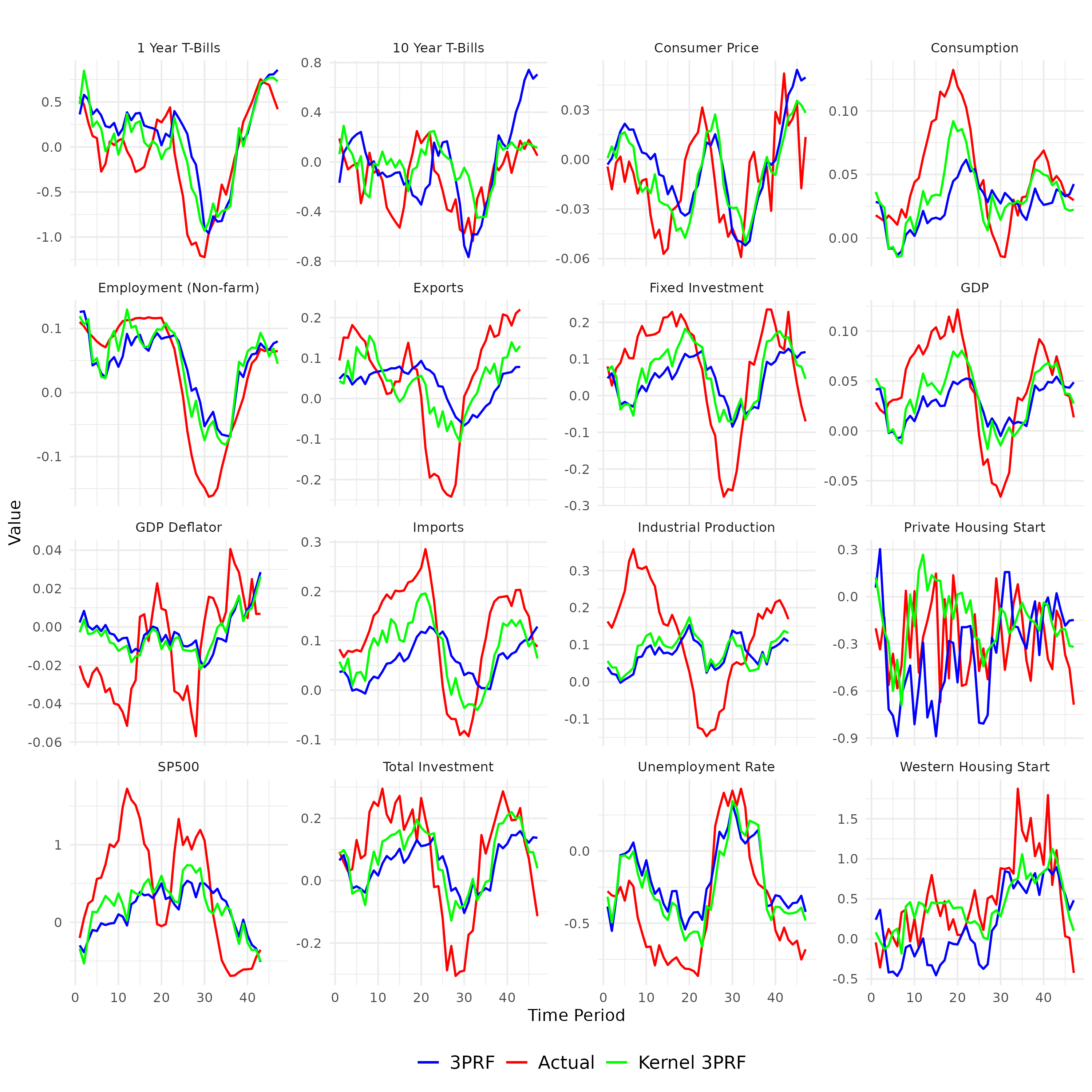
We plot the forecasts by our method and 3PRF method with the true value of the target series for all sixteen series discussed in the emprirical application section. To save some space, we only show the plots for one, four, eight, and twelve period ahead forecasts.


B.5 Comparative Performance on All Series For Each Horizons
| Analysis | Tolerance(%) | Methods | ||||||
|---|---|---|---|---|---|---|---|---|
| AR(2) | PCA | Sq-PC | PC-Sq | kPCA | 3PRF | k3PRF | ||
| h=1 | ||||||||
| 0 | 93.75 | 0.00 | 0.57 | 0.00 | 0.00 | 0.57 | 5.11 | |
| 5 | 95.45 | 1.70 | 0.00 | 0.57 | 0.57 | 5.11 | 11.93 | |
| 10 | 97.73 | 4.55 | 0.57 | 3.41 | 2.27 | 13.07 | 23.86 | |
| 20 | 97.73 | 13.07 | 3.41 | 14.20 | 4.55 | 23.86 | 49.43 | |
| h=2 | ||||||||
| 0 | 93.75 | 0.00 | 0.00 | 0.57 | 0.57 | 1.70 | 3.41 | |
| 5 | 95.45 | 1.14 | 0.00 | 1.70 | 0.57 | 4.55 | 8.52 | |
| 10 | 95.45 | 2.84 | 1.70 | 3.98 | 1.70 | 6.82 | 13.64 | |
| 20 | 96.59 | 9.09 | 2.84 | 10.80 | 4.55 | 16.48 | 40.91 | |
| h=3 | ||||||||
| 0 | 84.09 | 0.57 | 0.57 | 0.57 | 0.00 | 2.27 | 11.93 | |
| 5 | 89.20 | 1.70 | 1.14 | 2.27 | 0.00 | 3.98 | 19.89 | |
| 10 | 93.18 | 2.84 | 2.27 | 4.55 | 0.00 | 7.39 | 27.27 | |
| 20 | 94.89 | 6.25 | 3.41 | 9.66 | 1.70 | 17.61 | 47.16 | |
| h=4 | ||||||||
| 0 | 64.77 | 0.00 | 0.57 | 1.14 | 1.14 | 2.27 | 30.11 | |
| 5 | 68.18 | 1.14 | 1.70 | 1.70 | 1.14 | 6.82 | 34.66 | |
| 10 | 76.70 | 2.84 | 2.27 | 3.41 | 1.14 | 9.66 | 39.77 | |
| 20 | 88.07 | 5.11 | 3.98 | 6.82 | 3.41 | 22.16 | 57.39 | |
| h=6 | ||||||||
| 0 | 27.84 | 0.00 | 2.84 | 0.00 | 8.52 | 6.25 | 53.98 | |
| 5 | 29.55 | 0.00 | 3.98 | 1.70 | 9.66 | 7.95 | 58.52 | |
| 10 | 32.39 | 1.14 | 5.11 | 2.84 | 10.80 | 14.77 | 61.36 | |
| 20 | 40.91 | 5.11 | 6.82 | 7.39 | 14.20 | 25.00 | 70.45 | |
| h=8 | ||||||||
| 0 | 9.09 | 0.57 | 1.14 | 2.27 | 7.39 | 9.66 | 69.89 | |
| 5 | 9.66 | 2.27 | 1.70 | 2.84 | 8.52 | 11.36 | 70.45 | |
| 10 | 10.23 | 2.84 | 1.70 | 2.84 | 11.36 | 15.34 | 72.16 | |
| 20 | 11.36 | 3.41 | 4.55 | 5.11 | 13.07 | 28.41 | 78.98 | |
| h=10 | ||||||||
| 0 | 8.52 | 0.00 | 0.57 | 2.84 | 3.98 | 18.18 | 65.91 | |
| 5 | 8.52 | 0.00 | 1.14 | 2.27 | 3.98 | 19.89 | 67.61 | |
| 10 | 9.09 | 0.00 | 1.70 | 2.27 | 3.98 | 22.73 | 68.75 | |
| 20 | 9.66 | 1.14 | 2.27 | 3.98 | 7.95 | 29.55 | 73.30 | |
| h=12 | ||||||||
| 0 | 3.98 | 0.57 | 0.57 | 3.41 | 2.27 | 13.07 | 76.14 | |
| 5 | 4.55 | 1.14 | 1.14 | 2.84 | 2.27 | 13.64 | 76.70 | |
| 10 | 4.55 | 1.14 | 1.70 | 3.41 | 2.84 | 14.77 | 80.11 | |
| 20 | 6.25 | 2.27 | 2.27 | 3.98 | 4.55 | 23.30 | 82.95 | |