Sparse Sampling is All You Need for Fast Wrong-way Cycling Detection in CCTV Videos

Abstract.

In the field of transportation, it is of paramount importance to address and mitigate illegal actions committed by both motor and non-motor vehicles. Among those actions, wrong-way cycling (i.e., riding a bicycle or e-bike in the opposite direction of the designated traffic flow) poses significant risks to both cyclists and other road users. To this end, this paper formulates a problem of detecting wrong-way cycling ratios in CCTV videos. Specifically, we propose a sparse sampling method called WWC-Predictor to efficiently solve this problem, addressing the inefficiencies of direct tracking methods. Our approach leverages both detection-based information, which utilizes the information from bounding boxes, and orientation-based information, which provides insights into the image itself, to enhance instantaneous information capture capability. On our proposed benchmark dataset consisting of 35 minutes of video sequences and minute-level annotation, our method achieves an average error rate of a mere 1.475% while taking only 19.12% GPU time of straightforward tracking methods under the same detection model. This remarkable performance demonstrates the effectiveness of our approach in identifying and predicting instances of wrong-way cycling.

1. Introduction

Wrong-way cycling refers to the act of riding a bicycle or e-bike in the opposite direction of the designated traffic flow. It occurs when a cyclist travels against the established direction of travel for vehicles on a roadway or designated cycling path. This behavior poses significant safety risks for both cyclists and other road users, as it goes against established traffic rules and increases the likelihood of accidents and collisions.

With the emergence of the Internet of Things (IoT), many organizations and region governors install CCTV cameras in their responsible areas for surveillance and evidence recording. Traffic surveillance also enjoys the benefits of CCTV installation. Most CCTV cameras that record road traffic are likely to be installed and record the videos from the top view angle, from the skywalk, or from the electric poles, to allow the camera to record a wide angle of traffic roads. While the enforcement system for motor vehicles is robust — allowing police to issue fines based on clear evidence from CCTV footage — such detailed record-keeping is not necessary for non-motorized transport. However, assessing the frequency of wrong-way cycling through CCTV videos could provide essential data for law enforcement. This information helps gauge the safety level of specific areas, identifying zones with a high incidence of wrong-way cycling as potential targets for intensified surveillance. Therefore, our goal is to develop an efficient system capable of automatically calculating the wrong-way cycling ratio from CCTV footage, requiring minimal GPU resources.

In the literature, various approaches to wrong-way driving detection employ direct tracking methods. However, these methods have a significant limitation: they demand extensive GPU resources for processing a single video, making them inefficient and unnecessarily precise for our purposes. The extensive duration of CCTV footage and the sheer volume of data from numerous cameras necessitate a more resource-efficient solution. Additionally, a key distinction between these methods and our task lies in our specific requirements. Unlike tasks that require detailed processing, such as license plate recognition for punitive measures, our project only necessitates the prediction of a weak indicator – the wrong-way cycling ratio. This implies a considerable amount of redundant information exists between frames, suggesting the need for a more streamlined approach in our context.

To overcome this problem, we propose an algorithm called $\mathbf{W}$rong-$\mathbf{W}$ay $\mathbf{C}$ycling Predictor (WWC-Predictor) designed to efficiently make predictions using significantly fewer frames (6-10 times less) in videos. This is achieved through the implementation of a Two-Frame WWC Detector, which precisely extracts information from each sample. Following this, we deploy a Full-Time WWC Predictor that predicts time-dimensional information based on these extracts. By employing an ensemble model in a sparse manner and building a model grounded in this strategy, we can more efficiently estimate the likelihood of wrong-way cycling incidents.

Moreover, multi-object tracking (MOT) methods, especially those not based on detection (Chaabane et al., 2021; Chu et al., 2023; Zhang et al., 2021), require a substantial amount of labeled video data for model training. Annotating those videos is both time-consuming and costly, while contemporary open vocabulary models (Wang et al., 2023; Doersch et al., 2023) are not readily applicable in such specialized domains.

Another challenge arises from instantaneous tracking, whose unsteadiness can lead to potentially incorrect orientation detections by the detection model. To prevent misclassifications (both False Positives and True Negatives), we need a solution that goes beyond a simple detection-based tracking approach. In response, we introduce a multi-model ensemble strategy in our Two-Frame WWC Detector, depicted in Figure 1. This method adopts a consensus mechanism where discrepancies between the outputs of two models lead to the classification of an observation as invalid, enhancing the reliability of the system. Comprehensive details of this architecture are provided in Section 3.1. It acknowledges the complexity of vehicular movements, recognizing that not all detected vehicles can be neatly categorized. Through the integration of these models, we achieve a nuanced analysis and differentiation between instances of wrong-way cycling and scenarios where vehicles are stationary or moving backward due to crossroads or emergencies, ensuring a more accurate and robust detection system.

To evaluate our method, and to foster future research on this problem, we collect 405 annotated images for detection task, 1199 images for orientation detection task and 4 CCTV videos (35 minutes in total) for final validation. It should be noted that there is no data leakage between training and validation datasets.

In summary, this paper introduces WWC-Predictor, a novel algorithm designed to analyze CCTV footage with minimal frames, aiming to predict the probability of wrong-way cycling incidents effectively. Additionally, we establish the first benchmark dedicated to this specific downstream task. The source code and dataset will be released.

2. Related Work

2.1. Detection of Wrong-way Incidents

Wrong-way driving represents a closely related area that has garnered significant attention. Studies such as (Suttiponpisarn et al., 2022a; Shubho et al., 2021; Vardhan et al., 2023; Rahman et al., 2020; Suttiponpisarn et al., 2021; Manasa and Renuka Devi, 2023) have developed frameworks for the detection of wrong-way driving in CCTV footage. These frameworks employ a variety of multi-object tracking (MOT) methods, including FastMOT (Yang, 2020), DeepSORT (Wojke et al., 2017), Kalman filter(Saho, 2017) and centroid tracking (Rahman et al., 2020), to analyze vehicular movements. The approach detailed in (Suttiponpisarn et al., 2022a), which utilizes FastMOT, segments video footage into one-minute intervals. This segmentation allows for the precise identification of vehicle start and end points through tracking models, with subsequent post-processing to determine vehicle orientation. Contrarily, other strategies involve analyzing entire video sequences, employing detection-based methods followed by post-processing to ascertain the direction of travel. (Suttiponpisarn et al., 2021) and (Suttiponpisarn et al., 2022b) developed a system utilizing YOLOv4-tiny (Bochkovskiy et al., 2020) to detect object and DeepSORT tracking to track vehicles, in which two main algorithms called Road Lane Boundary detection from CCTV algorithm (RLB-CCTV) and Majority-Based Correct Direction Detection algorithm (MBCDD) are designed and improved to consume less computational time. (Choudhari et al., 2023) introduces a continuous tracking method for monitoring the direction of motorbikes, comparing it against the expected direction of the lane. If the tracked orientation of a motorbike is contrary to the lane direction for at least 80% of the observed time, it is identified as wrong-way riding. In essence, the prevailing strategies for detecting wrong-way incidents predominantly rely on tracking methods. While effective, these methods are noted for their time-intensive nature, underscoring a critical area for potential efficiency improvements.

It is also popular to utilize GPS information to detect wrong-way cycling. (Gu et al., 2017) proposes BikeMate, a ubiquitous bicycling behavior monitoring system with smartphones. (Hayashi et al., 2021) presented a mobile system that performed vision-based scene analysis to detect potentially dangerous cycling behavior including wrong-way cycling. (Dhakal et al., 2018) uses data collected from a smartphone application to explain wrong-way riding behavior of cyclists on one-way segments to help better identify the demographic and network factors influencing the wrong-way riding decision making.

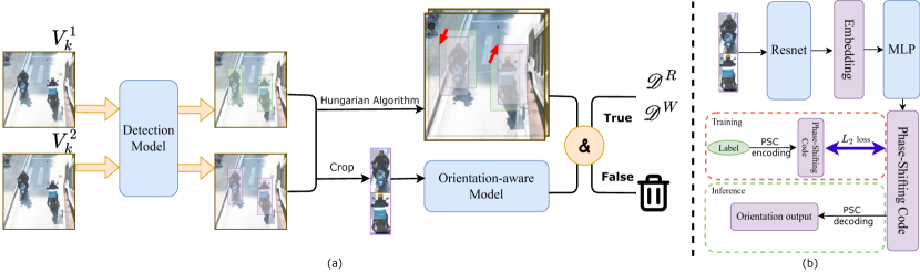
Figure 1. (a): Overview of Two-Frame Wrong-Way Cycling Detector, which consists of a detection model, an orientation-aware model and an And-strategy(shown as $\&$ on the figure). It takes two continuous frames as input, and output the amount of both right-way and wrong-way cycling. (b): Training and inference pipeline of our proposed orientation-aware model.

(a): Overview of Two-Frame Wrong-Way Cycling Detector, which consists of a detection model, an orientation-aware model and an And-strategy(shown as $\&$ on the figure). It takes two continuous frames as input, and output the amount of both right-way and wrong-way cycling. (b): Training and inference pipeline of our proposed orientation-aware model.

2.2. Orientation Detection

Originally, detecting the orientation of non-motor vehicles in videos poses a dynamic challenge. However, within our sparse analysis framework, this issue transitions into a more static scenario, prompting us to delve into orientation detection within still images. Although direct analogues—tasks with an image input leading to an orientation output—are scarce, there exists a foundation of architectures addressing orientation in various contexts. Historically, orientation challenges have often manifested within the realm of oriented object detection (Xie et al., 2021; Han et al., 2021; Wen et al., 2023). This methodology aims not only to delineate the object with a bounding box but also to ascertain its orientation, thereby enhancing the precision of detection beyond the capabilities of conventional object detection techniques.

A novel contribution to this field is introduced by (Yu and Da, 2023) through the development of a differentiable angle coder, termed the phase-shifting coder (PSC). This innovative approach tackles the issue of orientation cyclicity by translating the rotational periodicity across various cycles into the phase of differing frequencies, effectively addressing the rotation continuity problem. In our project, we incorporate the PSC to aid in resolving the challenges associated with orientation detection, leveraging its advanced capability to understand and quantify orientation within images accurately.

2.3. Model Ensemble

Ensemble learning (Ganaie et al., 2022) is a powerful technique that combines multiple individual models to achieve improved generalization performance. One approach to ensemble learning is multiple-model ensemble, where different models are fused together to enhance the performance of a specific task. The decision fusion strategy plays a crucial role in ensemble learning, as it determines how the outputs of the individual models are combined to achieve an effective ensemble.

There are several popular ensemble strategies that have been widely used. These include unweighted model averaging (Ju et al., 2018), majority voting (Kuncheva et al., 2003), stacked generation (Wolpert, 1992), among others. Each strategy has its own strengths and weaknesses, and the choice of strategy depends primarily on the specific task and dataset. In our targeted task, we have devised a novel yet efficacious combination strategy, termed the AND-Strategy, which capitalizes on the synergistic potential of the individual models to amplify the overall performance.

2.4. Mathematical Modeling of Traffic Flow

Given our focus on sparse time sequences, it is essential to establish connections among these sequences rather than treating them as isolated samples. The modeling of traffic flow serves as a pertinent example of this approach.

(Tian et al., 2021) suggests modeling the frequency components of network traffic using the ARMA model, illustrating a method to grasp the temporal dynamics in data. Similarly, (Peng et al., 2021) introduces an ARIMA-SVM combined prediction model to forecast urban short-term traffic flow, demonstrating the efficacy of integrating traditional statistical models with machine learning techniques for enhanced predictive accuracy. These methodologies underscore the significance of training models on a set of pre-measured network traffic data, enabling the ARMA or ARIMA-SVM models to capture the intrinsic characteristics of traffic flows and, subsequently, to forecast network traffic effectively. In our analysis, although prediction is not our primary aim, we employ similar techniques to distill specific features that elucidate the relationships among samples.

3. Method

3.1. Two-Frame Wrong-Way Cycling Detector

In this section, we are going to explain Two-Frame WWC detector, $M(.)$, which takes images as input and output amount of both right-way cycling and wrong-way cycling. Before that, we firstly symbolically explain how we obtain two-frame samples from videos.

The process begins by converting a given video, denoted as $\mathcal{V}$, into a series of sampled instances at regular intervals of $T_{gap}$ seconds, resulting in a sequence $(\mathcal{V}_{0},\mathcal{V}_{1},...)$. Every $V_{i}$ is a two-frame pair, which consists of two continuous frames. To quantify the cycling behavior within each sampled instance, we employ Two-Frame WWC Detector, where $M^{R}(.)$ and $M^{W}(.)$ respectively measure the number of right-way and wrong-way cycling occurrences. The application of these functions to the video sequence yields two corresponding time series datasets: $\mathcal{D}^{R}=(M^{R}(\mathcal{V}_{0}),M^{R}(\mathcal{V}_{1}),...)$ and $\mathcal{D}^{W}=(M^{W}(\mathcal{V}_{0}),M^{W}(\mathcal{V}_{1}),...)$.

1

0:  whole dataset $\mathcal{V}$, right-way orientation $O_{right}$

1:  for $\mathcal{V}_{k}$ in $\mathcal{V}$ do

2:     $\mathbf{B}\leftarrow D(\mathcal{V}_{k})$

3:     $\mathbf{X}_{\textit{iou}}\leftarrow F_{\textit{iou}}(\mathbf{B}_{1},\mathbf{B}_{2})$

4:     $\mathbf{X}_{\textit{iou}}\leftarrow(\mathbf{X}_{\textit{iou}}<\textit{IoU}_{\textit{max}})\cdot\mathbf{X}_{\textit{iou}}$

5:     $L_{\textit{match}}\leftarrow\mathbf{H}(\mathbf{X}_{\textit{iou}})$

6:     for $i,j$ in $L_{\textit{match}}$ do

7:        $O_{\textit{det}}\leftarrow\mathbf{Orient}(\mathbf{Cen}(\mathbf{B}_{1}^{i}),\mathbf{Cen}(\mathbf{B}_{2}^{j}))$

8:        $O_{\textit{model}}\leftarrow\mathbf{Ave}(\mathbf{F}_{o}({\mathbf{B}_{1}^{i},\mathcal{V}_{k}^{1}}),\mathbf{F}_{o}({\mathbf{B}_{2}^{j},\mathcal{V}_{k}^{2}}))$

9:        if $\mathbf{AndStrategy}(O_{\textit{det}},O_{\textit{model}})$ then

10:           $Ans.\mathbf{append}(\mathbf{Ave}(O_{\textit{det}},O_{\textit{model}}))$

11:        end if

12:     end for

13:  end for

14:  $is\_Right\leftarrow\textbf{Dis}(Ans,O_{right})<120$

15:  $\mathcal{D}^{R}\leftarrow\mathbf{SUM}(is\_Right)$

16:  $\mathcal{D}^{W}\leftarrow\mathbf{SUM}(\neg is\_Right)$

17:  return  $\mathcal{D}^{R},\mathcal{D}^{W}$

Algorithm 1 Two-Frame Wrong-Way Cycling Detector

We divide our Two-Frame WWC Detector into three parts, detection, orientation prediction and ensemble strategy. Pseudo code is shown in Algorithm 1.

In the beginning, a pair of consecutive frames $\mathcal{V}_{i}$ are inferred by a detection model, which can be represented as $\mathbf{B}=D(\mathcal{V}_{i})$, where $D$ represents the detection function and $\mathbf{B}$ represents the output bounding boxes. In this case, we utilize YOLOv5(Jocher, 2020) as our chosen detection model. $F_{iou}$ is a function used to compute an Intersection over Union (IoU) matrix between two lists of bounding boxes. The expression $Out=\mathbf{X}_{iou}<IoU_{max}$ represents a boolean matrix where $Out^{i,j}$ is zero when $\mathbf{X}_{iou}^{i,j}<IoU_{max}$, and one otherwise. This is implemented to exclude certain stable vehicles from being considered. Then, we apply Hungarian algorithm, denoted as function $H$, to match bipartite graph where each side represents bounding boxes in one of the two frames. Function $H$ returns a list of several pairs of matched index which is saved as $L_{match}$. For each match get by Hungarian algorithm, we firstly count a detection-based orientation by computing the direction of center point in bounding box:

(1) $$\mathbf{v} =C_{2}-C_{1},$$

$$O_{det} =\text{arctan2}(\mathbf{v}_{y},\mathbf{v}_{x}),$$

where $C_{i}$ denotes the central point of the bounding box in the $i$-th frame.

In the subsequent phase, an orientation-aware model, denoted as $F_{o}$, is employed to distill orientation information from the image data. This model processes cropped images obtained from bounding boxes identified through the Hungarian algorithm. It then yields an average orientation prediction, $O_{model}$, for the images across consecutive frames. The intricacies of $F_{o}$ are further elucidated in Section 3.2.

Following this, an ensemble strategy integrates the outputs from both the detection process and the orientation-aware model. This step involves assessing whether $O_{det}$ and $O_{model}$ adhere to the And-strategy. Specifically, if the absolute difference between $O_{det}$ and $O_{model}$ is less than the predefined threshold, $\text{Div}{max}$, the output is deemed valid; otherwise, it is rejected. This threshold, $\text{Div}{max}$, acts as a critical super-parameter to guarantee alignment between $O_{det}$ and $O_{model}$. Valid outputs are subsequently averaged to ascertain the final orientation measure.

The last stage entails calculating the distance between $Ans$ and $O_{right}$. A distance of less than 120 degrees is classified as a right-way cycling instance; otherwise, it is considered wrong-way cycling. The procedure culminates in the quantification of right-way cycling, $\mathcal{D}^{R}$, and wrong-way cycling, $\mathcal{D}^{W}$, instances.

Mathematically, it can be demonstrated that employing an And-strategy with an ensemble of two models can significantly enhance overall performance compared to relying on a singular model. We provide the mathematical proof in supplementary.

3.2. Orientation-aware Model

An orientation-aware model takes an image of vehicle as input, and output its facing orientation. Its architecture can be seen in Figure 1. Since the model aim to predict the objects’ orientation, a continuous and periodic variable, we applied Phase-Shifting Coder(PSC) (Yu and Da, 2023) to transform the discontinuous degree system into continuous $m$-dimention vector. In our work, we assign $m$ as $3$. The PSC works as follows:

Encoding:

(2) $$x_{i}=\cos\left(\varphi+\frac{2i\pi}{m}\right),i=1,2,\cdots,m.$$

Decoding:

(3) $$\varphi=-\arctan\frac{\sum^{m}_{i=1}x_{i}\sin(\frac{2i\pi}{m})}{\sum^{m}_{i=1}x_{i}\cos(\frac{2i\pi}{m})}.$$

More specifically, we apply pretrained backbone, Resnet-101(He et al., 2016) here, to generate embedding $\mathbf{b}\in\mathbb{R}^{n}$ for an image, and a linear layer is applied to convert the embedding $\mathbf{b}$ to vector $\hat{\mathbf{x}}\in\mathbb{R}^{m}$.

During training process, the label $\varphi\in\left(-\pi,\pi\right]$ is encoded to $\mathbf{x}\in\mathbb{R}^{m}$. Then the loss is computed as follows:

(4) $$l=\frac{1}{m}\|\hat{\mathbf{x}}-\mathbf{x}\|^{2}.$$

During inference, the vector $\hat{\mathbf{x}}\in\mathbb{R}^{m}$ is decoded to $\hat{\varphi}\in\left(-\pi,\pi\right]$ as the final output.

In the orientation prediction task, we define the metric as the distance between the prediction and the label. Since it is a cyclic number, its formula can be expressed as:

(5) $$d=\max(\varphi,\hat{\varphi})-\min(\varphi,\hat{\varphi}).$$

$$\text{Error}=\left\{\begin{array}[]{l}d,\quad\text{if }d\leq 180,\\ 360-d,\quad\text{otherwise}.\end{array}\right.$$

Here, $\varphi$ represents the label value and $\hat{\varphi}$ represents the predicted value. Both $\varphi$ and $\hat{\varphi}$ are in the range of $(0,360]$ and are measured in degrees. The error is computed based on the difference between the maximum and minimum values of $\varphi$ and $\hat{\varphi}$. If this difference is less than or equal to 180 degrees, the error is equal to $d$. Otherwise, if the difference is greater than 180 degrees, the error is computed as $360-d$.In the experimental part, we utilize this metric to evaluate the performance of our model.

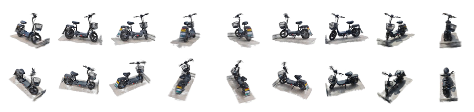
Figure 2. One case reconstructed and generated by instant-ngp.

One case reconstructed and generated by instant-ngp.

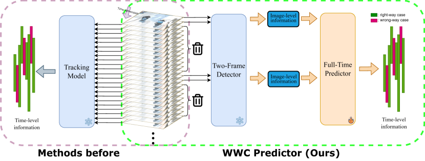
Figure 3. Comparison between our proposed WWC Predictor and previous tracking-based dense sampling pipeline.

To train our orientation-aware model, we utilize an effective pretrain-finetune architecture. Recognizing the challenges associated with obtaining real-world data with precise orientation labels and addressing long-tail attributes, we generate synthetic data. This synthetic data serves as a means to pretrain the model and provide it with a beneficial bias towards orientation information. By leveraging this approach, we aim to enhance the model’s ability to understand and utilize orientation cues in real-world scenarios.

Firstly, we capture 360-degree videos using a regular camera in real-world settings. We then capture 30-40 frames from the video and utilize a trained COLMAP(Schönberger et al., 2016; Schönberger and Frahm, 2016) (Structure-from-Motion and Multi-View Stereo) system to estimate the camera’s position and attitude parameters both inside and outside the captured scenes. Using these information, we reconstruct a 3D model using instant-ngp(Müller et al., 2022).

Next, we leverage pre-designed camera poses to render images with corresponding orientation labels. To simulate real-world conditions, we render images from different heights for each orientation as shown in Figure 2.

This process enables us to create a diverse dataset comprising labeled images, which serves as valuable pretraining data for our orientation-aware model. In total, we conducted 12 3D models, resulting in 864 images used for pretraining. After pretraining, the whole model is finetuned by real-world data.

3.3. Full-Time Wrong-Way Cycling Predictor

In this section, we describe Full-Time WWC Predictor architecture for transforming from sparse time-sequenced information into full-time samples for the analysis of cycling patterns, specifically focusing on distinguishing between right-way and wrong-way cycling instances.

Given the complexity of establishing a direct relationship between these time-sequenced datasets and a specific ratio over a defined period, we propose a modeling approach to bridge the gap between image-level and time-level information. This approach assumes that the counts of right-way ($N^{R}$) and wrong-way ($N^{W}$) cycling instances going through at regular intervals of $T_{gap}$ seconds can be approximated by Poisson distributions. This assumption allows us to estimate the proportion of wrong-way cycling as

(6) $$Ratio=\frac{E(N^{W})}{E(N^{R})+E(N^{W})},$$

where $E(N^{W})$ and $E(N^{R})$ represent the expected values of wrong-way and right-way cycling instances, respectively. The challenge then becomes determining how to express $N$ (the total number of instances going through in $T_{gap}$) using the available time series data $\mathcal{D}$. $E(N)$ and samples of $N$ will be derived in the following.

We observe that $N_{t}$ can be represented by the count of new vehicles identified in $\mathcal{D}_{t}$ relative to $\mathcal{D}_{t-1}$ when the sampling interval $T_{gap}$ is small enough to ensure some degree of overlap between consecutive samples. In this context, we propose a parameter $\varphi$, which quantifies the probability of a vehicle from the previous sample persisting into the subsequent one, becoming particularly relevant. While this approach may introduce some level of uncertainty in individual samples due to the dynamic nature of vehicle movement and detection within short intervals, it is considered effective for large-scale analysis. Formally, we have:

(7) $$\hat{N}_{k}=\mathcal{D}_{k}-\varphi\mathcal{D}_{k-1}$$

To effectively estimate the parameter $\varphi$, we employ the Auto Regressive Moving Average (ARMA) model. ARMA model can be generally described as following:

(8) $$\mathcal{D}_{k}=c+\epsilon_{k}+\sum\limits_{i=1}^{p}\varphi_{i}\mathcal{D}_{k-i}+\sum\limits_{i=1}^{q}\theta_{j}\epsilon_{k-j}$$

The ARMA model is a blend of two components, the Auto Regressive (AR) part and the Moving Average (MA) part.

Constant Term ($c$) is the intercept of the model which affects all predictions with a constant shift. In our scenario, it means the average number of vehicles appearing in timestamp $k$ compared with $k-1$.

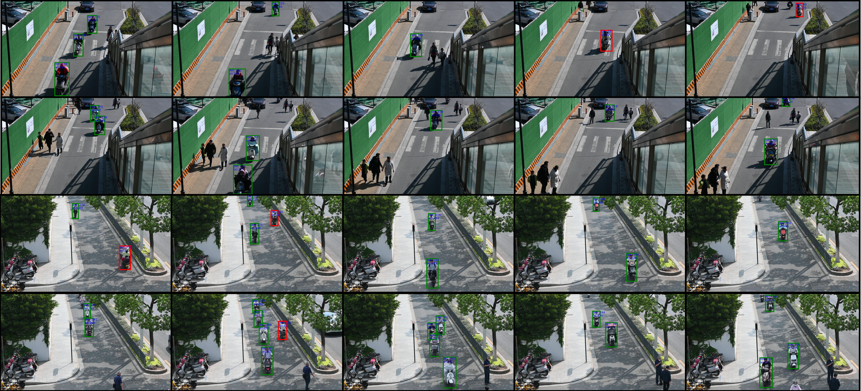
Figure 4. Visualization from the validation videos for wrong-way cycling prediction in video, where green bounding box means right-way cycling, red means wrong-way cycling. ’Det’ and ’Ori’ means output orientation from detection branch or orientation-aware branch.

Error Term ($\epsilon_{t}$) is the error term at time $t$, which captures random fluctuations in the time series that are not explained by the past values. $\epsilon_{t}$ is expected to obey Gaussian distribution with mean value of zero since it is a random fluctuations. In our scenario, it means the random fluctuations of vehicles in each sampling.

The sum $\Sigma_{i=1}^{p}\varphi_{i}\mathcal{D}_{k-i}$ is the auto regression (AR) part of the model, where $p$ is the order of the AR process. Each $\varphi_{i}$ is a parameter that multiplies the number of vehicles at a previous time point $k-i$, indicating how past values are weighted in the model. In our scenario, $p$ is selected as one, so that this can be shorted as $\varphi\mathcal{D}_{k-i}$, which means expected number that remain from the last sample to current sample.

The expression $\Sigma_{i=1}^{q}\theta_{j}\epsilon_{k-j}$ represents the moving average (MA) component, wherein $q$ denotes the order of the MA process. Each coefficient $\theta_{j}$ corresponds to a parameter that is applied to the lagged error term $\epsilon_{k-j}$, illustrating the impact of historical forecast errors on the current value. Within our traffic flow context, this encapsulates the momentum of vehicular movement, particularly in scenarios involving right-way cycling. Conversely, for instances of wrong-way cycling, which are irregular and unforeseen, the MA component is disregarded, thereby setting $q$ to zero.

Originally, the purpose of the ARMA model is to develop a predictive model capable of forecasting future values in a time series by learning from its historical observations (AR component) and the errors in past predictions (MA component). In our context, we specifically utilize the $\varphi$ parameter to bridge the gap between image-level data $\mathcal{D}$ and the time-level counts $N$. We apply maximum likelihood estimation (MLE) to estimate $\varphi$, whose details can be seen in (Perktold et al., 2023; McLeod and Zhang, 2008).

Through this approach, we are able to derive sets of $\hat{N}^{R}$ and $\hat{N}^{W}$, which can be treated as independent samples from a Poisson distribution. Subsequently, we apply the maximum likelihood estimation (MLE) technique to both $N^{R}$ and $N^{W}$. The probability density function is expressed as:

(9) $$P(N=n)=\frac{\lambda^{n}e^{-\lambda}}{n!}.$$

Furthermore, the estimation of the parameter $\lambda$ (which is also the expected value) is given by:

(10) $$E(N)=\lambda=\frac{1}{m}\sum\limits_{i=1}^{m}n_{i},$$

enabling the computation of the final ratio as depicted in Equation 6.

4. Experiments

4.1. Proposed datasets

Taking all factors into consideration, we propose three distinct datasets for different purposes. These datasets include the orientation-aware dataset, the detection training dataset, and the final validation dataset. Each dataset serves a specific role in our model development and evaluation process.

4.1.1. Orientation-aware Dataset

The orientation-aware dataset is designed specifically for training the orientation-aware model. This dataset comprises three subsets: the pretraining set, the finetuning set, and the validation set.

The pretraining set consists of synthetic images generated using instant-ngp. It includes 12 distinct 3D models, and for each model, we generate 72 labeled images captured from two different heights, as depicted in Figure 2. In total, the pretraining set contains 864 images.

The finetuning set consists of real-world images labeled by detection method and adjusted by hand, some of which shown in Figure 5. There are 1060 images in finetuning set and 139 images in validation set.

	Long		Short 1		Short 2		Short 3		Overall	GAP	GPU Time per Minute
	Ratio	Error	Ratio	Error	Ratio	Error	Ratio	Error	Error
Ours	14.8%	+3.6%	3.9%	-0.6%	3.6%	+1.1%	4.9%	+0.6%	1.475%	2s	4.50s
	16.6%	+5.4%	2.7%	-1.8%	2.1%	-0.4%	3.8%	-0.5%	2.025%	4s	2.95s
Ours(detection only)	17.3%	+6.1%	11.9%	+7.4%	6.2%	+3.7%	11.8%	+7.5%	6.20%	2s	3.83s
SORT(Bewley et al., 2016)	12.2%	+1.0%	4.2%	-0.3%	2.4%	-0.1%	4.1%	-0.2%	0.375%	0.17s	20.18s
DeepSORT(Wojke et al., 2017)	11.5%	+0.3%	3.8%	-0.7%	2.4%	-0.1%	4.1%	-0.2%	0.325%	0.17s	29.37s
ByteTrack(Zhang et al., 2022)	12.1%	+0.9%	4.3%	-0.2%	2.5%	+0.0%	4.1%	-0.2%	0.325%	0.17s	24.11s
	14.3%	+3.1%	3.0%	-1.5%	7.7%	+5.2%	1.6%	-2.7%	3.12%	0.5s	15.85s

Table 1. Statistical Comparison of Our Method Against Others Using Our Benchmark. ”Error” refers to the absolute deviation between the predicted ratio and the ground truth, while ”Overall Error” represents the mean of these four discrepancies. ”Gap” denotes the temporal interval between successive samples in this methodology.

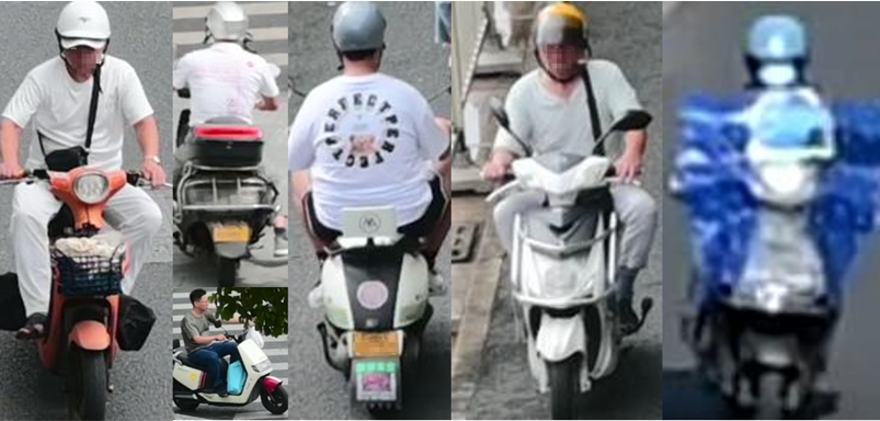
Figure 5. Cases of real-world images in finetuning set and validation set.

4.1.2. Detection dataset

For the training and validation of the detection model, we construct a training set and a validation set. There is only one class in this dataset which is non-motor vehicle. These sets consist of a total of 223 pictures captured in different conditions, encompassing 474 effective bounding boxes. The split ratio between the training set and the validation set is 8:2, and all the results from our experiments are based on this ratio. Our experiments have verified that this volume of data is sufficient for effectively training a detection model.

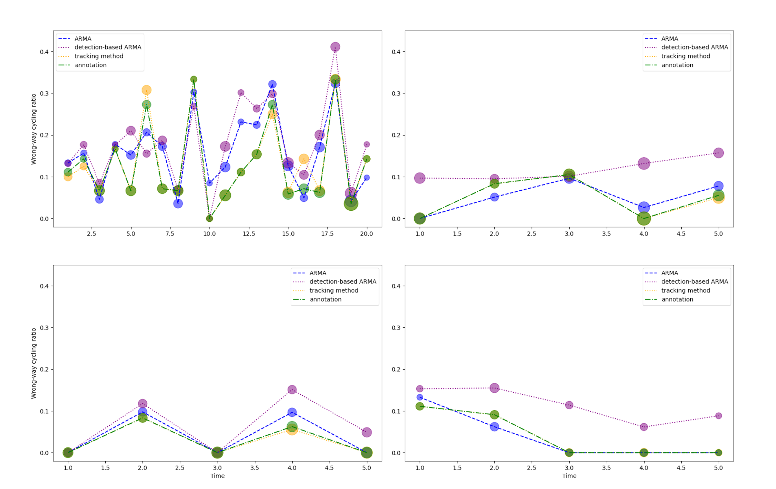
Figure 6. Minute-level comparison between WWC-Predictor, detection-only WWC-predictor, and tracking-based method(SORT). The size of circle showcases its scale of number.

4.1.3. Final Validation Dataset

To establish a robust evaluation metric, we collect four videos captured by road cameras situated at varied locations: three 5-minute videos and one 20-minute video. These videos form the foundation for assessing the performance of different methods in terms of both speed and accuracy. By incorporating a diverse array of video footage, as depicted in Figure 4, we ensure a comprehensive evaluation of the methods across different real-world conditions. Furthermore, we annotate instances of wrong-way and right-way cycling every minute, enabling us to assess performance on a minute-by-minute basis. This evaluation strategy allows us to determine the effectiveness and reliability of various methods in accurately and efficiently predicting the ratio of wrong-way cycling in road camera videos.

4.2. Results

To showcase the strength of proposed WWC-Predictor, we have established two kinds of baselines: the single detection-based method and the traditional tracking-based method as shown in Table 1. The detection-only WWC-Predictor follows a similar pipeline to our ensemble method, where we consider the orientation ($O_{det}$) between the center points of the two bounding boxes as the final output. In the case of the tracking baseline, given that only a detection model is available, we are limited to tracking-by-detection methods. For this purpose, we employ SORT(Bewley et al., 2016), DeepSORT(Wojke et al., 2017) and currently SOTA tracking method, ByteTrack(Zhang et al., 2022) as the tracking baseline. In DeepSORT, our orientation-aware model serves as a feature extractor. Specifically, we utilize YOLOv5-m as the detection model, and a finetuned Resnet-101 coupled with a Phase-Shifting Coder serves as the orientation-aware model. The interval between two sampling points is set to 2 seconds, and the skip time between two consecutive frames is fixed at 0.02 second, corresponding to a frame rate of 30 fps for continuous video frames.

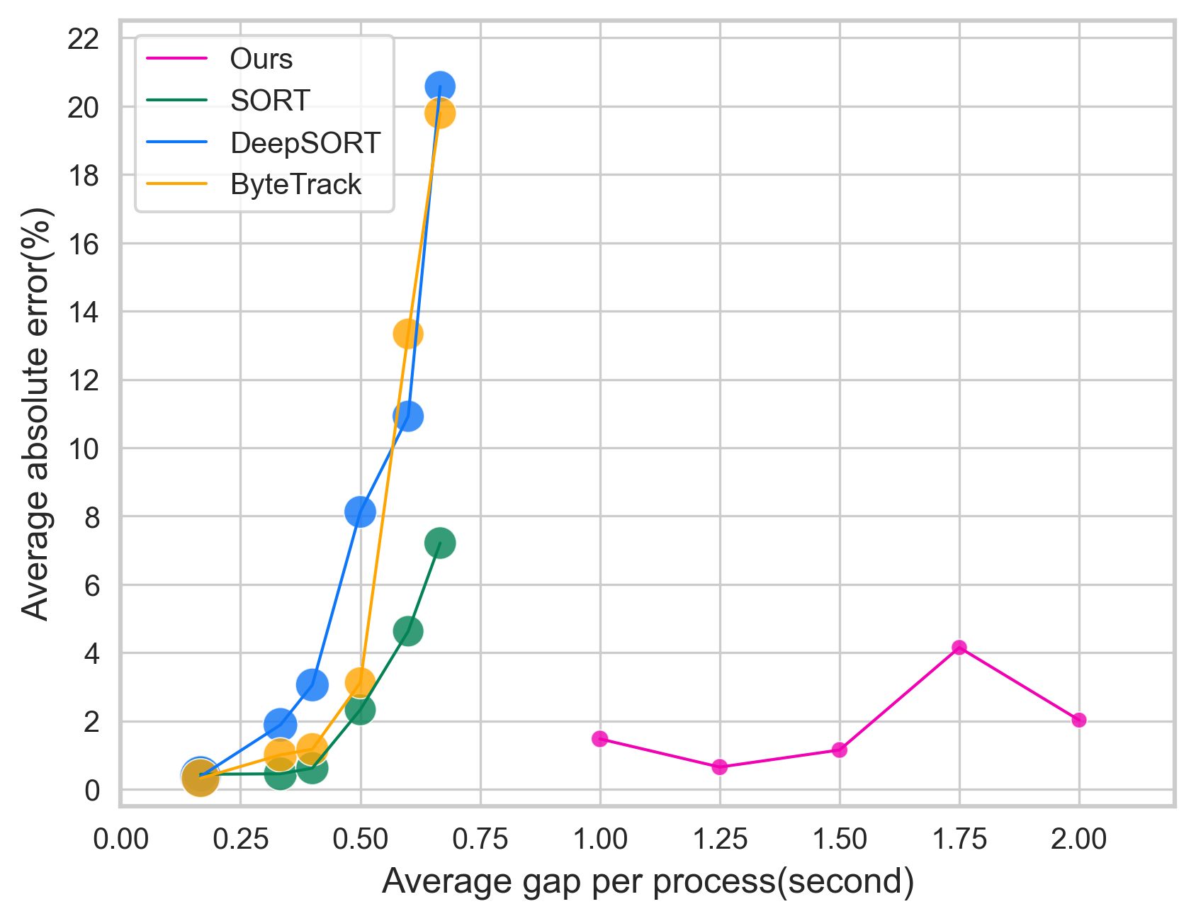
Figure 7. Processed information scale, algorithm speed and performance comparison between WWC-Predictor, SORT, DeepSORT and ByteTrack. The size of circle showcases algorithm speed.

To demonstrate the effectiveness of our proposed WWC-Predictor, we have established two baseline methodologies: a single detection-based approach and a traditional tracking-based approach, as delineated in Table 1. The detection-based WWC-Predictor adheres to a pipeline analogous to our composite method, wherein the orientation ($O_{det}$) between the centroids of the bounding boxes is regarded as the ultimate output. Regarding the tracking baseline, constrained by the availability of only a detection model, we resort to tracking-by-detection strategies. To this end, we integrate SORT(Bewley et al., 2016) and DeepSORT(Wojke et al., 2017) as our tracking frameworks. Within DeepSORT, our orientation-aware model, functions as a feature extractor. In particular, we deploy YOLOv5-m as the detection architecture, while a refined Resnet-101 in conjunction with a Phase-Shifting Coder is utilized as the orientation-sensitive model. We set the temporal interval between sampling instances at 2/4 seconds, and the inter-frame skip duration is maintained at 0.02 seconds, equating to a video frame rate of 30 fps for seamless video sequences.

Table 1 presents a statistical comparison of our method against the baselines on our benchmark dataset. GPU processing time was measured on a single RTX 3080Ti, with serial inference for the detection model and parallel inference for the orientation model (in cases processing a single image). Figure 6 presents a minute-level comparison between those three methods.

Overall, the comprehensive WWC-Predictor method exhibits a competitive absolute error rate of 1.475% and a swift inference time of 4.50 seconds per video minute. The detection-only variant of WWC-Predictor demonstrates a higher error margin due to the inherent uncertainty of the detection model, which leads to a significant proportion of True-Negative errors. Conversely, the traditional tracking method showcases a lower error rate owing to its robust frame-to-frame relations and the simplicity of time-dimensional prediction at the expense of substantially higher computational resource requirements.

Figure 7 presents a comparative analysis of the WWC Predictor against SORT and DeepSORT across varying time interval scales. It is evident that both SORT and DeepSORT require relatively short time intervals to maintain effective tracking, whereas our WWC Predictor demonstrates robust performance over a specific range of larger intervals. Contrary to expectations, the WWC Predictor does not deliver optimal results at the smallest interval. We provide an explanation for this phenomenon: at lower intervals, the probability, denoted by $\varphi$, that vehicles will continue in the same direction from one sample to the next is significantly high, necessitating precise prediction of $\varphi$. Consequently, any failure in accurately predicting the $\varphi$ for either correct or incorrect vehicle direction could compromise the overall prediction accuracy.

Model	AP0.50:0.95	AP0.5	AP0.75
TOLOv5-small	0.728	0.959	0.911
YOLOv5-medium	0.764	0.973	0.929

Table 2. AP scores of our YOLOv5 trained on our dataset for different IOU thresholds.

Table 2 presents the performance metrics of our detection model applied to a custom dataset. These results underscore the efficacy of our detection system for static scenes. Moreover, they hint that the sub-optimal performance of WWC-Prediction in video analysis stems from the inherent complexities of dynamic environments rather than the detection model’s capabilities.

4.3. Ablation Study

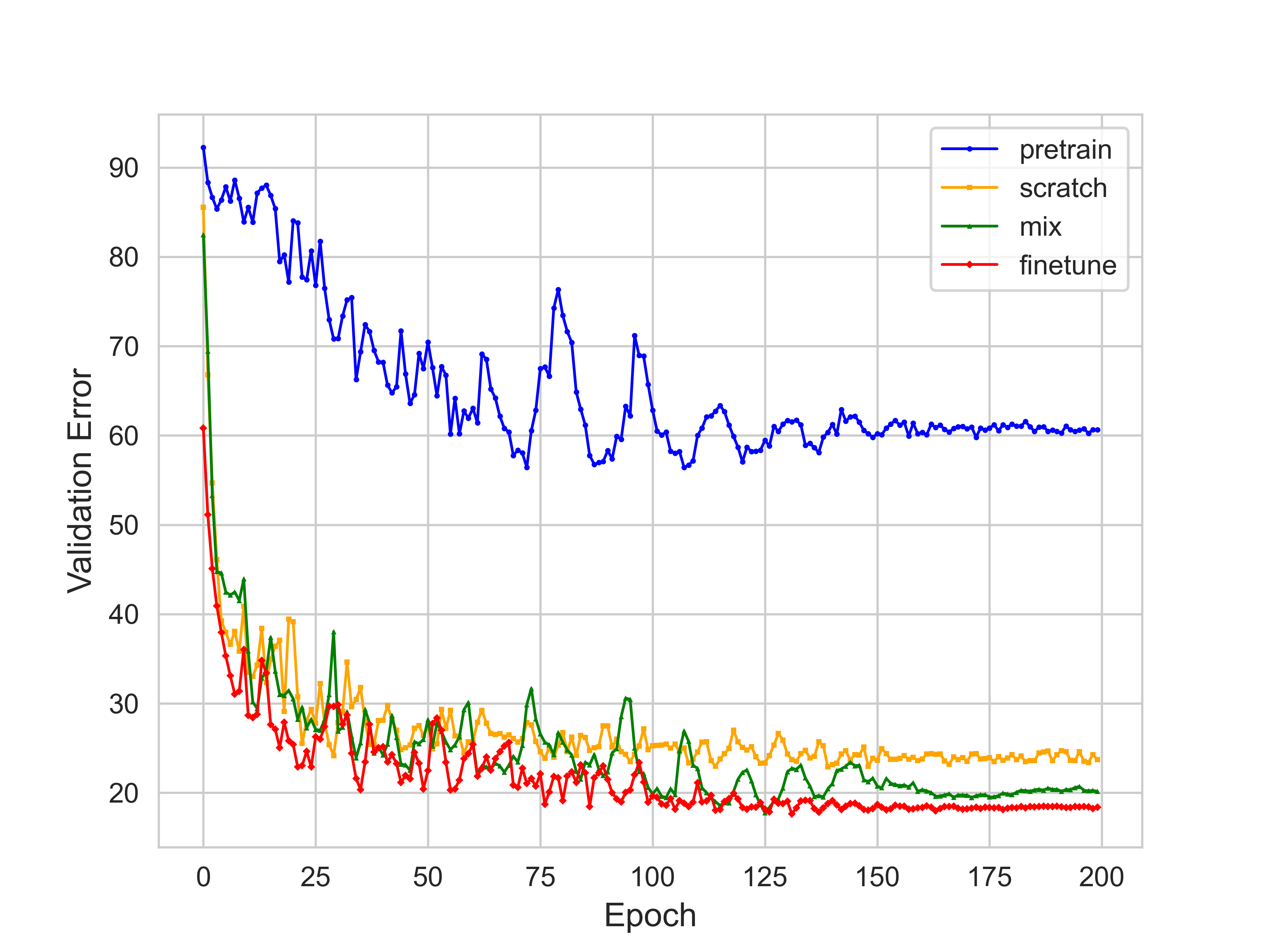
Figure 8. Comparison of different training strategy for orientation-aware model.

4.3.1. Ablation on orientation-aware model

As described in Section 3.2, we have devised a pretrain-finetune architecture for training an orientation-aware model. To evaluate the impact of the pretraining dataset and this specific training architecture, we conducted an ablation study. This study allowed us to assess the effectiveness and significance of these components in our model’s performance.

Comparison of the validation error changes resulting from different training methods is presented in Figure 8. The training methods are categorized as follows:

• ”Pretrain” denotes training exclusively with synthetic data.

• ”Scratch” refers to training solely with real-world data.

• ”Mix” represents training by combining both real-world and synthetic data.

• ”Finetune” indicates the process of fine-tuning on real-world data following a pretraining phase with synthetic data.

In our pretrain-finetune architecture, we successfully attain a minimal validation error of 17.63. Moreover, the performance post-convergence significantly surpasses that of training from scratch or employing a mixed dataset. While this error rate might initially appear substantial, it is deemed acceptable for its intended application as a verification model.

5. Conclusion

In this paper, we introduced the new problem of wrong-way cycling ratio prediction in CCTV videos, and proposed a novel method, WWC-Predictor, to tackle this problem by sparse sampling with efficient Two-Frame WWC-Detector and Full-Time WWC-Predictor, which has been mathematically and experimentally proven to be effective compared with straightforward tracking methods. Additionally, to facilitate the training and validation of our method for this task, we have presented and open-sourced three datasets to build a convincing benchmark of this task.

However, it is important to note that this task still requires further research and exploration. Our experiments on minute-level annotated video suggest that WWC-Predictor shows a performance relatively weaker than that in Long-Form video. We attribute it to a global predicted $\varphi$, but if we do not do so, a minuscule number of samples in minute can not predict $\varphi$ well. We consider it a good direction to optimize the method of this kind of few-shot occasion. Also, WWC-Predictor is a off-line pipeline. Thus, online wrong-way cycling ratio prediction can be a good topic and can be of great use.

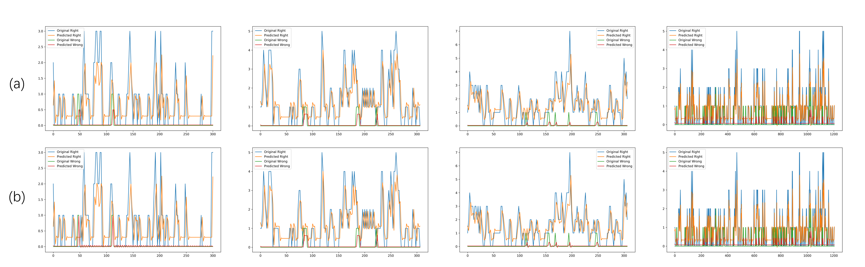
Figure 9. In (a), we use ARMA(1,1) model to fit right-way cycling cases, while ARMA(1,0) for wrong-way cycling cases. In (b), use ARMA(1,1) model to fit both wrong-way cycling cases and right-way cycling cases.

	ARMA model for Right-way cycling						ARMA model for Wrong-way cycling
	AR			MA			AR			MA
	std err	z	P>—z—	std err	z	P>—z—	std err	z	P>—z—	std err	z	P>—z—
Long	0.048	10.783	0.000	0.055	3.800	0.000	0.071	6.094	0.000	0.083	-1.021	0.307
Short 1	0.093	6.143	0.000	0.107	1.832	0.067	0.087	6.583	0.000	0.080	0.504	0.614
Short 2	0.130	3.428	0.001	1.320	1.482	0.138	0.316	-0.015	0.988	0.282	3.512	0.000
Short 3	0.095	5.857	0.000	0.115	1.603	0.109	0.491	-0.146	0.884	0.470	0.751	0.453
Ave	0.092	6.553	0.000	0.399	2.179	0.079	0.241	3.129	0.468	0.229	0.937	0.344

Table 3. Statistic results of auto regression(AR) part and moving average(MA) part for right-way cycling and wrong-way cycling.

Appendix A Mathematical proof of And-strategy

In this section, we present a mathematical proof of the effectiveness of our proposed And-strategy. This proof demonstrates that when the accuracy of both models exceeds 50%, employing this strategy results in superior performance.

Lemma A.1.

Assume that $P_{1}$ and $P_{2}$ represent the respective posterior probabilities that each of the two models errs, which are in the range of $(0,0.5]$, $P_{w}=P_{1}P_{2}$ represents the possibility of two models erring simultaneously, and $P_{valid}=(1-P_{1})(1-P_{2})+P_{1}P_{2}$ represents the possibility of the sample being valid. The possibility of the ensemble model erring $P_{3}=\frac{P_{w}}{P_{valid}}\leq min\{P_{1},P_{2}\}$.

Proof.

Considering $P_{3}$ as a function related to $P_{1},P_{2}$, we have

(11) $$P_{3}=f(P_{1},P_{2})=\frac{P_{1}P_{2}}{(1-P_{1})(1-P_{2})+P_{1}P_{2}}$$

Deriving $f$ with respect to $P_{1}$ (or equivalently $P_{2}$) yields:

(12) $$\frac{\partial f}{\partial P_{1}} =\frac{-P_{2}^{2}+P_{2}}{(1-P_{1}-P_{2}+2P_{1}P_{2})^{2}},$$

$$\frac{\partial f}{\partial P_{1}} >0,\ \text{for}\ P_{1},P_{2}\in(0,0.5].$$

This establishes $P_{3}$ as a monotonically increasing function relative to $P_{1}$ and $P_{2}$. As a result,

(13) $$P_{3}\leq f(P_{1},0.5)=P_{1},P_{3}\leq f(0.5,P_{2})=P_{2}.$$

∎

Appendix B experiments of ARMA part

In this section, we conduct a series of experiments to evaluate the performance of the Auto Regressive Moving Average (ARMA) model in the context of predicting wrong-way cycling occurrences. Figure 9 illustrates a comparative analysis between the ARMA(1,0) and ARMA(1,1) configurations. The notation ARMA($p$, $q$) denotes an ARMA model where $p$ is the order of the auto regressive (AR) process, and $q$ is the order of the moving average (MA) process.

The analysis, particularly evident in the first and third panels of subfigure (b), suggests that the inclusion of the MA component, which originally intended to capture traffic flow dynamics, does not contribute positively to the predictive accuracy for wrong-way cycling events. This is attributed to the observation that wrong-way cycling incidents rarely exhibit the traffic flow characteristics modeled by the MA component.

Table 3 presents the respective standard errors, z-values, and p-values for auto regressive (AR) and moving average (MA) terms from ARMA models applied to two different cycling behaviors: Right-Way Cycling and Wrong-way Cycling. In the ARMA model analysis for cycling behaviors, the ”Short 2” category within the Wrong-way Cycling data exhibits an unusual case where the AR term appears completely non-significant with a p-value of 0.988, indicating a misinterpretation of the auto regressive effect as if it were a moving average component. Generally, for Wrong-way Cycling, the AR terms consistently show non-significance across all categories, suggesting a lack of moving average characteristic in this behavior. This pattern contrasts with the Right-way cycling data, where AR terms are significant, indicating a reliable auto regressive process.

To address this discrepancy, we incorporate domain knowledge into the model specification process. Consequently, we refine the ARMA model for wrong-way cycling prediction to an ARMA(1,0) configuration, effectively omitting the MA component. This adjustment is predicated on the rationale that the auto regressive component alone is more representative of the underlying process governing wrong-way cycling incidents, thereby enhancing the model’s predictive relevance in this particular application.

References

- (1)
- Bewley et al. (2016) Alex Bewley, Zongyuan Ge, Lionel Ott, Fabio Ramos, and Ben Upcroft. 2016. Simple Online and Realtime Tracking. In 2016 IEEE International Conference on Image Processing (ICIP). https://doi.org/10.1109/icip.2016.7533003
- Bochkovskiy et al. (2020) Alexey Bochkovskiy, Chien-Yao Wang, and Hong-Yuan Mark Liao. 2020. Yolov4: Optimal speed and accuracy of object detection. arXiv preprint arXiv:2004.10934 (2020).
- Chaabane et al. (2021) Mohamed Chaabane, Peter Zhang, J Ross Beveridge, and Stephen O’Hara. 2021. Deft: Detection embeddings for tracking. arXiv preprint arXiv:2102.02267 (2021).
- Choudhari et al. (2023) Rutvik Choudhari, Shubham Goel, Yash Patel, and Sunil Ghane. 2023. Traffic Rule Violation Detection using Detectron2 and Yolov7. In 2023 World Conference on Communication & Computing (WCONF). IEEE, 1–7.
- Chu et al. (2023) Peng Chu, Jiang Wang, Quanzeng You, Haibin Ling, and Zicheng Liu. 2023. Transmot: Spatial-temporal graph transformer for multiple object tracking. In Proceedings of the IEEE/CVF Winter Conference on applications of computer vision. 4870–4880.
- Dhakal et al. (2018) Nirbesh Dhakal, Christopher R Cherry, Ziwen Ling, and Mojdeh Azad. 2018. Using CyclePhilly data to assess wrong-way riding of cyclists in Philadelphia. Journal of safety research 67 (2018), 145–153.
- Doersch et al. (2023) Carl Doersch, Yi Yang, Mel Vecerik, Dilara Gokay, Ankush Gupta, Yusuf Aytar, Joao Carreira, and Andrew Zisserman. 2023. Tapir: Tracking any point with per-frame initialization and temporal refinement. In Proceedings of the IEEE/CVF International Conference on Computer Vision. 10061–10072.
- Ganaie et al. (2022) M.A. Ganaie, Minghui Hu, A.K. Malik, M. Tanveer, and P.N. Suganthan. 2022. Ensemble deep learning: A review. Engineering Applications of Artificial Intelligence (Oct 2022), 105151. https://doi.org/10.1016/j.engappai.2022.105151
- Gu et al. (2017) Weixi Gu, Zimu Zhou, Yuxun Zhou, Han Zou, Yunxin Liu, Costas J Spanos, and Lin Zhang. 2017. Bikemate: Bike riding behavior monitoring with smartphones. In Proceedings of the 14th eai international conference on mobile and ubiquitous systems: Computing, networking and services. 313–322.
- Han et al. (2021) Jiaming Han, Jian Ding, Nan Xue, and Gui-Song Xia. 2021. ReDet: A Rotation-equivariant Detector for Aerial Object Detection. In 2021 IEEE/CVF Conference on Computer Vision and Pattern Recognition (CVPR). https://doi.org/10.1109/cvpr46437.2021.00281
- Hayashi et al. (2021) Hirotaka Hayashi, Anran Xu, Zhongyi Zhou, and Koji Yatani. 2021. Vision-based scene analysis toward dangerous cycling behavior detection using smartphones. In Adjunct Proceedings of the 2021 ACM International Joint Conference on Pervasive and Ubiquitous Computing and Proceedings of the 2021 ACM International Symposium on Wearable Computers. 28–29.
- He et al. (2016) Kaiming He, Xiangyu Zhang, Shaoqing Ren, and Jian Sun. 2016. Deep Residual Learning for Image Recognition. In 2016 IEEE Conference on Computer Vision and Pattern Recognition (CVPR). https://doi.org/10.1109/cvpr.2016.90
- Jocher (2020) Glenn Jocher. 2020. YOLOv5 by Ultralytics. https://doi.org/10.5281/zenodo.3908559
- Ju et al. (2018) Cheng Ju, Aurélien Bibaut, and Mark van der Laan. 2018. The relative performance of ensemble methods with deep convolutional neural networks for image classification. Journal of Applied Statistics (Nov 2018), 2800–2818. https://doi.org/10.1080/02664763.2018.1441383
- Kuncheva et al. (2003) Ludmila Kuncheva, Chris Whitaker, C.A. Shipp, and Robert Duin. 2003. Limits on the majority vote accuracy in classier fusion. Formal Pattern Analysis & Applications 6 (04 2003), 22–31. https://doi.org/10.1007/s10044-002-0173-7
- Manasa and Renuka Devi (2023) A Manasa and SM Renuka Devi. 2023. An Enhanced Real-Time System for Wrong-Way and Over Speed Violation Detection Using Deep Learning. In International Conference on Image Processing and Capsule Networks. Springer, 309–322.
- McLeod and Zhang (2008) A Ian McLeod and Ying Zhang. 2008. Faster ARMA maximum likelihood estimation. Computational Statistics & Data Analysis 52, 4 (2008), 2166–2176.
- Müller et al. (2022) Thomas Müller, Alex Evans, Christoph Schied, and Alexander Keller. 2022. Instant Neural Graphics Primitives with a Multiresolution Hash Encoding. ACM Transactions on Graphics (Jul 2022), 1–15. https://doi.org/10.1145/3528223.3530127
- Peng et al. (2021) Jiaxin Peng, Yongneng Xu, and Menghui Wu. 2021. Short-Term Traffic Flow Forecast Based on ARIMA-SVM Combined Model. In International Conference on Green Intelligent Transportation System and Safety. Springer, 287–300.
- Perktold et al. (2023) Josef Perktold, Skipper Seabold, Kevin Sheppard, ChadFulton, Kerby Shedden, jbrockmendel, j grana6, Peter Quackenbush, Vincent Arel-Bundock, Wes McKinney, Ian Langmore, Bart Baker, Ralf Gommers, yogabonito, s scherrer, Yauhen Zhurko, Matthew Brett, Enrico Giampieri, yl565, Jarrod Millman, Paul Hobson, Vincent, Pamphile Roy, Tom Augspurger, tvanzyl, alexbrc, Tyler Hartley, Fernando Perez, Yuji Tamiya, and Yaroslav Halchenko. 2023. statsmodels/statsmodels: Release 0.14.1. https://doi.org/10.5281/zenodo.10378921
- Rahman et al. (2020) Zillur Rahman, Amit Mazumder Ami, and Muhammad Ahsan Ullah. 2020. A Real-Time Wrong-Way Vehicle Detection Based on YOLO and Centroid Tracking. In 2020 IEEE Region 10 Symposium (TENSYMP). 916–920. https://doi.org/10.1109/TENSYMP50017.2020.9230463
- Saho (2017) Kenshi Saho. 2017. Kalman filter for moving object tracking: Performance analysis and filter design. Kalman Filters-Theory for Advanced Applications (2017), 233–252.
- Schönberger and Frahm (2016) Johannes Lutz Schönberger and Jan-Michael Frahm. 2016. Structure-from-Motion Revisited. In Conference on Computer Vision and Pattern Recognition (CVPR).
- Schönberger et al. (2016) Johannes Lutz Schönberger, Enliang Zheng, Marc Pollefeys, and Jan-Michael Frahm. 2016. Pixelwise View Selection for Unstructured Multi-View Stereo. In European Conference on Computer Vision (ECCV).
- Shubho et al. (2021) Fahimul Hoque Shubho, Fahim Iftekhar, Ekhfa Hossain, and Shahnewaz Siddique. 2021. Real-time traffic monitoring and traffic offense detection using YOLOv4 and OpenCV DNN. In TENCON 2021-2021 IEEE Region 10 Conference (TENCON). IEEE, 46–51.
- Suttiponpisarn et al. (2021) Pintusorn Suttiponpisarn, Chalermpol Charnsripinyo, Sasiporn Usanavasin, and Hiro Nakahara. 2021. Detection of Wrong Direction Vehicles on Two-Way Traffic. In 2021 13th International Conference on Knowledge and Systems Engineering (KSE). 1–6. https://doi.org/10.1109/KSE53942.2021.9648579
- Suttiponpisarn et al. (2022a) Pintusorn Suttiponpisarn, Chalermpol Charnsripinyo, Sasiporn Usanavasin, and Hiro Nakahara. 2022a. An autonomous framework for real-time wrong-way driving vehicle detection from closed-circuit televisions. Sustainability 14, 16 (2022), 10232.
- Suttiponpisarn et al. (2022b) Pintusorn Suttiponpisarn, Chalermpol Charnsripinyo, Sasiporn Usanavasin, and Hiro Nakahara. 2022b. An enhanced system for wrong-way driving vehicle detection with road boundary detection algorithm. Procedia Computer Science 204 (2022), 164–171.
- Tian et al. (2021) Miao Tian, Chen Sun, and Shaozhi Wu. 2021. An EMD and ARMA-based network traffic prediction approach in SDN-based internet of vehicles. Wireless Networks (2021), 1–13.
- Vardhan et al. (2023) M. Harsha Vardhan, K. Venkata Sai Krishna, Sunitha Munappa, and K. Aditya Manoj. 2023. Wrong Route Vehicles Detection Using Deep Learning. In 2023 International Conference on Next Generation Electronics (NEleX). 1–6. https://doi.org/10.1109/NEleX59773.2023.10421458
- Wang et al. (2023) Qianqian Wang, Yen-Yu Chang, Ruojin Cai, Zhengqi Li, Bharath Hariharan, Aleksander Holynski, and Noah Snavely. 2023. Tracking everything everywhere all at once. In Proceedings of the IEEE/CVF International Conference on Computer Vision. 19795–19806.
- Wen et al. (2023) Long Wen, Yu Cheng, Yi Fang, and Xinyu Li. 2023. A comprehensive survey of oriented object detection in remote sensing images. Expert Systems with Applications 224 (2023), 119960. https://doi.org/10.1016/j.eswa.2023.119960
- Wojke et al. (2017) Nicolai Wojke, Alex Bewley, and Dietrich Paulus. 2017. Simple online and realtime tracking with a deep association metric. In 2017 IEEE International Conference on Image Processing (ICIP). https://doi.org/10.1109/icip.2017.8296962
- Wolpert (1992) David Wolpert. 1992. Stacked Generalization. Neural Networks 5 (12 1992), 241–259. https://doi.org/10.1016/S0893-6080(05)80023-1
- Xie et al. (2021) Xingxing Xie, Gong Cheng, Jiabao Wang, Xiwen Yao, and Junwei Han. 2021. Oriented R-CNN for Object Detection. In 2021 IEEE/CVF International Conference on Computer Vision (ICCV). https://doi.org/10.1109/iccv48922.2021.00350
- Yang (2020) Yukai Yang. 2020. FastMOT: High-Performance Multiple Object Tracking Based on Deep SORT and KLT. https://doi.org/10.5281/zenodo.4294717
- Yu and Da (2023) Yi Yu and Feipeng Da. 2023. Phase-Shifting Coder: Predicting Accurate Orientation in Oriented Object Detection. In Proceedings of the IEEE/CVF Conference on Computer Vision and Pattern Recognition (CVPR). 13354–13363.
- Zhang et al. (2022) Yifu Zhang, Peize Sun, Yi Jiang, Dongdong Yu, Fucheng Weng, Zehuan Yuan, Ping Luo, Wenyu Liu, and Xinggang Wang. 2022. Bytetrack: Multi-object tracking by associating every detection box. In European conference on computer vision. Springer, 1–21.
- Zhang et al. (2021) Yifu Zhang, Chunyu Wang, Xinggang Wang, Wenjun Zeng, and Wenyu Liu. 2021. Fairmot: On the fairness of detection and re-identification in multiple object tracking. International Journal of Computer Vision 129 (2021), 3069–3087.