Adaptive-TMLE for the Average Treatment Effect based on Randomized Controlled Trial Augmented with Real-World Data

Abstract

We consider the problem of estimating the average treatment effect (ATE) when both randomized control trial (RCT) data and real-world data (RWD) are available. We decompose the ATE estimand as the difference between a pooled-ATE estimand that integrates RCT and RWD and a bias estimand that captures the conditional effect of RCT enrollment on the outcome. We introduce an adaptive targeted minimum loss-based estimation (A-TMLE) framework to estimate them. We prove that the A-TMLE estimator is $\sqrt{n}$-consistent and asymptotically normal. Moreover, in finite sample, it achieves the super-efficiency one would obtain had one known the oracle model for the conditional effect of the RCT enrollment on the outcome. Consequently, the smaller the working model of the bias induced by the RWD is, the greater our estimator’s efficiency, while our estimator will always be at least as efficient as an efficient estimator that uses the RCT data only. A-TMLE outperforms existing methods in simulations by having smaller mean-squared-error and 95% confidence intervals. A-TMLE could help utilize RWD to improve the efficiency of randomized trial results without biasing the estimates of intervention effects. This approach could allow for smaller, faster trials, decreasing the time until patients can receive effective treatments.

1 Introduction

The 21st Century Cures Act, enacted by the United States Congress in 2016, was designed to enhance the development process of drugs and medical devices through the use of real-world evidence (RWE), aiming to expedite their availability to patients in need [1]. In response, the U.S. Food and Drug Administration (FDA) released a framework in 2018 for its Real-World Evidence Program, providing comprehensive guidelines on the use of RWE to either support the approval of new drug indications or satisfy post-approval study requirements [2]. This framework highlighted the incorporation of external controls, such as data from previous clinical studies or electronic health records, to strengthen the evidence gathered from randomized controlled trials (RCTs), especially when evaluating the safety of an already approved drug for secondary outcomes. Combining RCT data with external real-world data (RWD) would potentially allow for a more efficient and precise estimation of treatment effects, especially if the drug had been approved in specific regions, making data on externally treated patients also available. However, this hybrid design of combining RCT and RWD, sometimes referred to as data fusion or data integration, faces challenges, including differences in the trial population versus the real-world population, which may violate the positivity assumption. Researchers often employ matching techniques to balance patient characteristics between the trial and real-world [3]. Furthermore, existing methods often rely on the assumption of mean exchangeability over the studies, as described in [4, 5], which states that enrolling in the RCT does not affect patients’ mean potential outcomes, given observed baseline characteristics. However, this assumption may not hold in reality, if, for example, being in the RCT setting increases patients’ adherence to their assigned treatment regimes.

In the absence of additional assumptions, investigators are limited to using data from the RCT alone (or a well-designed observational study without unmeasured confounding), completely ignoring the external data sources. However, efficient estimators could still utilize the external data to obtain useful scores from the covariates as dimension reductions to be used in the primary study, which might improve their finite sample performance, although from an asymptotic perspective an efficient estimator can totally ignore the external data. On the other hand, if investigators are willing to make assumptions about the impact of being enrolled in the RCT on the outcome of interest, conditioned on treatment and covariates, then the resulting new statistical model would allow for construction of efficient estimators that are significantly more precise than an estimator ignoring the external study data. Such a model would allow investigators to estimate the bias of the combined causal effect estimand.

Making unrealistic assumptions will generally cause biased inference, thereby destroying the sole purpose of the RCT as the gold-standard and a study that can provide unbiased estimates of the desired causal effect. To address this problem, we propose an estimation framework that data-adaptively learns a statistical working-model that approximates the true impact of the study indicator on the outcome (which represents the bias function for the external study) and then constructs an efficient estimator for the working-model-specific-ATE estimand, defined as the projection of the true data distribution onto the working model, based on the combined data. Our method follows precisely the general adaptive targeted minimum loss-based estimation (A-TMLE) proposed in [6]. A-TMLE has been shown to be asymptotically normal for the original target parameter, under the same assumptions as a regular TMLE (assuming that one uses a sensible nonparametric method for model selection such as choosing among many candidate working models via cross-validation), but with a super-efficient influence function that equals the efficient influence function of the target parameter when assuming an oracle model that is approximated by the data-adaptive working model. In our particular setting of augmenting RCT finding with RWD, a regular TMLE would always be asymptotically normal by only using the RCT data asymptotically. Therefore, the A-TMLE would asymptotically fully preserve the robustness of the regular TMLE of the true target parameter. Moreover, A-TMLE equals to a well-behaved TMLE of the working-model-specific-ATE estimand, which is itself of interest, beyond that its approximation error with respect to the true target estimand is of second-order. One may view A-TMLE as a way to regularize the efficient TMLE by performing bias-variance trade-off in an adaptive fashion. Specifically, in our setting, the more complex the true impact of the study indicator on the outcome as a function of the treatment and baseline covariates, the larger the data-adaptive working model would be. Hence, the gain in efficiency of the A-TMLE is driven by the complexity of the bias function. Interestingly, even if the bias is large in magnitude but is easily approximated by a function of the treatment and baseline covariates, A-TMLE will still achieve a large gain in efficiency.

To summarize our contributions, A-TMLE provides valid nonparametric inference in problems of integrating RCT data and RWD while fully utilizing the external data. These estimators are not regular with respect to the original statistical model but are regular under the oracle submodel. As sample size grows, the data-adaptively learned working model will eventually approximate the true model, but in finite sample A-TMLE acts as a super-efficient estimator of the true parameter and efficient estimator of the projection parameter. In our particular estimation problem where even efficient estimators could be underpowered, this class of A-TMLE provides a way forward to achieve more efficiency gain in finite sample without sacrificing nonparametric consistency and valid statistical inference. Although we give up some regularity along perturbation paths of the data distribution that fall outside the learned submodel, the oracle submodel includes only relevant perturbations of the data distribution, so such loss of regularity is not a problem. Nonetheless, since the data-adaptive working model approximates the oracle model, going for a larger working model than what cross-validation suggests might result in finite sample bias reductions. Therefore, in practice, one might also consider strategies including undersmoothing [7] or enforcing a minimal working model (e.g. a main-term only minimal working model) to further protect against finite sample bias.

1.1 Related Work

The decision to integrate or discard external data in the analysis of an RCT often hinges on whether pooling introduces bias. A simple “test-then-pool” strategy involves first conducting a hypothesis test to determine the similarity between the RCT and RWD before deciding to pool them together or rely solely on the RCT data [8]. The threshold of the test statistic above which the hypothesis test would be rejected could be determined data-adaptively [9]. However, methods of this type can be limited by the small sample sizes typical of RCTs, potentially resulting in underpowered hypothesis tests [10]. Additionally, using the “test-then-pool” strategy, either an efficiency gain is realized, or it is not, without gradation. Bayesian dynamic borrowing methods adjust the weight of external data based on the bias it introduces [11, 12, 13, 14, 15]. Similar frequentist approaches data-adaptively choose between data sources by balancing the bias-variance trade-off, often resulting in a weighted combination of the RCT-only and the pooled-ATE estimands [16, 17, 18]. In particular, the experiment-selector cross-validated targeted maximum likelihood estimator (ES-CVTMLE) method [16] also allow the incorporation of a negative control outcome (NCO) in the selection criteria. The gain in efficiency of these methods largely depends on the bias magnitude, with larger biases diminishing efficiency gains. Other methods incorporate a bias correction by initially generating a biased estimate, then learning a bias function, and finally adjusting the biased estimate to achieve an unbiased estimate of the causal effect, which has a similar favor to the method we are proposing [19, 20, 21]. However, the key aspect distinguishing our work and theirs is that their techniques rely on the independence between potential outcomes and the study indicator $S$ given observed covariates, an assumption that could easily be violated in reality. For instance, subjects might adhere more strictly to assigned treatment regimens had they been enrolled in the RCT, so being in the RCT or not modifies the treatment effects. These methods also focus primarily on unmeasured confounding bias, yet other biases, such as differences in outcome measurement or adherence levels between RCT and RWD settings, may also occur. The reliance on this independence assumption also limits their applicability in scenarios involving surrogate outcomes in the RWD, in which case the outcomes in the RCT and RWD are either measured differently or are fundamentally different variables, a common scenario one would encounter in practice. We define our bias directly as the difference between the target estimand and the pooled estimand, therefore it covers any kind of bias, including unmeasured confounding bias. Thus, our method can be applied more broadly, even in cases where the outcomes differ in the two studies.

1.2 Organization of the article

This article is organized as follows. In Section 2 we formally define the estimation problem in terms of the statistical model and target estimand that identifies the desired average treatment effect. In Section 3, we decompose our target estimand into a difference between a pooled-ATE estimand $\tilde{\Psi}$ and a bias estimand $\Psi^{\#}$. In Sections 4 and 5, we provide the key ingredients for constructing A-TMLEs of $\Psi^{\#}$ and $\tilde{\Psi}$ respectively. In Section 4, we present the semiparametric regression working model for the conditional effect of the study indicator on the outcome and the corresponding projection parameter $\Psi^{\#}_{{\cal M}_{w,2}}$ that replaces the outcome regression by its $L^{2}$-projection onto the working model $\mathcal{M}_{w,2}$. This then defines a working-model-specific target estimand on the original statistical model and thus defines a new estimation problem that would approximate the desired estimation problem if the working model approximates the true data density. If the study indicator has zero impact on the outcome, then the pooled-ATE estimand that just combines the data provides a valid estimator, thereby allowing full integration of the external data into the estimator; If the study indicator has an impact explained by a parametric form (e.g. a linear combination of a finite set of spline basis functions), then the estimand still integrates the data but carries out a bias correction according to this parametric form. As the parametric form becomes nonparametric, the estimand becomes the estimand that ignores the outcome data in the external study when estimating the outcome regression, corresponding with an efficient estimator. We derive the canonical gradient and the corresponding TMLE of the projection parameter $\Psi^{\#}_{{\cal M}_{w,2}}$. Similarly, in Section 5, we present a semiparametric regression working model for the pooled-ATE estimand $\tilde{\Psi}$ and define the corresponding projection parameter. In this case the semiparametric regression model learns the conditional effect of the treatment (instead of the study indicator) on the outcome, conditioned on treatment and baseline covariates, while not conditioning on the study indicator. The projection is defined as the $L^{2}$-projection of the true outcome regression $E_{P}(Y\mid A,W)$ (ignoring the study indicator) onto the working model $\mathcal{M}_{w,1}$. We present the canonical gradient and the corresponding TMLE of $\tilde{\Psi}_{{\cal M}_{w,1}}$. We summarize our A-TMLE algorithm in Section 6. Specifically, using a synthetic example, we illustrate how one might apply A-TMLE to augment RCT with external data in practice. In Section 7 we analyze the A-TMLE analogue to [6], to make this article self-contained. The analysis can be applied to both components of the target parameter, thereby also providing an asymptotic linearity theorem for the resulting A-TMLE of the target parameter. Specifically, we prove that the A-TMLEs of $\Psi^{\#}$ and $\tilde{\Psi}$ are $\sqrt{n}$-consistent, asymptotically normal with super-efficient variances. Under an asymptotic stability condition for the working model, they are also asymptotically linear with efficient influence functions that equal the efficient influence functions of the limit of the submodel (oracle model). In Section 8, we carry out simulation studies to evaluate the performance of our proposed A-TMLE against other methods including ES-CVTMLE [16], PROCOVA (a covariate-adjustment method) [22], a regular TMLE for the target estimand, and a TMLE using RCT data alone. We conclude with a discussion in Section 9.

2 The Estimation Problem

We observe $n$ independent and identically distributed observations of the random variable $O=(S,W,A,Y)\sim P_{0}\in\mathcal{M}$, where $P_{0}$ is the true data-generating distribution and $\mathcal{M}$ is the statistical model. We use $S\in\{0,1\}$ for the indicator of the unit belonging to a well-designed study with no unmeasured confounding, e.g. an RCT, where the causal effect of the treatment on the outcome can be identified; $W$ is a vector of baseline covariates measured at enrollment; $A\in\{0,1\}$ is an indicator of being in the treatment arm; $Y$ is the final clinical outcome of interest. Note that for the external data, we consider two scenarios, one with only external control arm and the other with both external treatment and external control arms. The problem formulation and estimation are generally the same for those two scenarios. We will make additional remarks at places where there are differences.

2.1 Structural causal model

We assume a structural causal model (SCM): $S=f_{S}(U_{S})$; $W=f_{W}(S,U_{W})$; $A=f_{A}(S,W,U_{A})$; $Y=f_{Y}(S,W,A,U_{Y})$, where $U=(U_{S},U_{W},U_{A},U_{Y})$ is a vector of exogenous errors. The joint distribution of $(U,O)$ is parametrized by a vector of functions $f=(f_{S},f_{W},f_{A},f_{Y})$ and the error distribution $P_{U}.$ The SCM ${\cal M}^{F}$ is defined by assumptions on these functions and the error distribution. Here ${\cal M}^{F}$ denotes the set of full data distributions $P_{U,O}$ that satisfy these assumptions on $f$ and $P_{U}$. The SCM allows us to define the potential outcomes $Y_{1}=f_{Y}(S,W,A=1,U_{Y})$ and $Y_{0}=f_{Y}(S,W,A=0,U_{Y})$ by intervening on the treatment node $A$.

2.2 Statistical model

We make the following three assumptions:

1. $(Y_{0},Y_{1})\perp A\mid S=1,W$ (randomization in the RCT);

2. $0<P(A=1\mid S=1,W)<1,P_{W}\text{-a.e.}$ (positivity of treatment assignment in the RCT);

3. $P(S=1\mid W)>0,P_{W}\text{-a.e.}$ (positivity of RCT enrollment in the pooled population).

Assumption A1 is a causal assumption and is non-testable, assumptions A2 and A3 are statistical assumptions. Note that assumptions A1 and A2 are satisfied in an RCT (or a well-designed observational study). Importantly, we do not make the assumption that $E(Y_{a}\mid S=0,W)=E(Y_{a}\mid W)$, sometimes referred to as the “mean exchangeability over $S$” [5]. In other words, for the combined study, $A$ might not be conditionally independent of $Y_{0},Y_{1}$, given $W$, due to the bias introduced from the external data. Specifically, we are concerned that $E_{W}E(Y_{1}-Y_{0}\mid W)\not=E_{W}E(Y\mid W,A=1)-E_{W}E(Y\mid W,A=0)$, due to $E_{W}E(Y_{1}-Y_{0}\mid W,S=0)\not=E_{W}E(Y\mid S=0,W,A=1)-E_{W}E(Y\mid S=0,W,A=0)$. Beyond these three assumptions, we will make additional assumptions on $g_{0}(1\mid S,W)\equiv P(A=1\mid S,W).$ In particular, if $S=1$ corresponds with an RCT, then $g_{0}(1\mid S=1,W)$ would just be the randomization probability; If the $S=1$-study is not an RCT, we might still be able to make a conditional independence assumption $g_{0}(A\mid 1,W)=g_{0}(A\mid 1,W_{1})$ for some subset $W_{1}$ of $W$. In some cases, we might also be able to assume that $S$ is independent of $W$, i.e. $P_{W\mid S=1}=P_{W\mid S=0}.$ This independence could be achieved by sampling the external subjects from the same target population as in the $S=1$-study. As we will see later in the identification step, for our target parameter it is crucial that the support of $P_{W\mid S=0}$ is included in the support of $P_{W\mid S=1}$ so that assumption A3 holds. In this article we will not make assumptions on the joint distribution of $(S,W)$ beyond assumption A3, but our results are not hard to generalize to the case that we assume $W\perp S$. In the important case that we augment an RCT with external controls only we have that $g_{0}(1\mid 0,W)=0$, so that the only purpose of the $S=0$-study is to augment the control arm of the RCT. To briefly summarize, we do not make any additional assumptions beyond the same set of assumptions for a standard RCT. The only additional assumption we require is A3 and could be made plausible in the selection of the external subjects.

Let ${\cal M}$ be the set of possible distributions $P$ of $O$ that satisfies the statistical assumptions A2 and A3. Then, ${\cal M}=\{P_{P_{U,O}}:P_{U,O}\in{\cal M}^{F}\}$ is the model implied by the full data model ${\cal M}^{F}$. We can factorize the density of $O$ according to the time-ordering as follows:

$$p(s,w,a,y)=p_{S}(s)p_{W}(w\mid s)g_{A}(a\mid s,w)q_{Y}(y\mid s,w,a),$$

where $q_{Y}(y\mid s,w,a)\equiv p_{Y}(y\mid s,w,a).$ Our statistical model only makes assumptions on $g_{A}$ and leaves the other factors in the likelihood unspecified.

2.3 Target causal parameters

We could consider two candidate target parameters. The first one is

$$\Psi^{F}(P_{O,U})=E_{W}E(Y_{1}-Y_{0}\mid S=1,W).$$

Note that this parameter measures the conditional treatment effect in the RCT, while it takes an average with respect to the combined covariate distribution $p_{W}=p_{W\mid S=1}p_{S=1}+p_{W\mid S=0}p_{S=0}$. Alternatively, we could take the average with respect to the RCT covariate distribution $p_{W\mid S=1}$, in which case we have the target parameter given by

$$\Psi^{F}_{2}(P_{O,U})=E(Y_{1}-Y_{0}\mid S=1)=E_{W}[E(Y_{1}-Y_{0}\mid S=1,W)\mid S=1].$$

In the following subsections, we will discuss the their identification results and compare their efficient influence functions.

2.4 Statistical estimand

Under assumptions A1, A2 and A3, the full-data target causal parameter $\Psi^{F}$ is identified by the following statistical target parameter $\Psi:{\cal M}\rightarrow\hbox{${\rm I\kern-1.99997ptR}$}$ defined by

$$\Psi(P_{0})=E_{0}[E_{0}(Y\mid S=1,W,A=1)-E_{0}(Y\mid S=1,W,A=0)].$$

Note that this estimand is only well-defined if $\min_{a\in\{0,1\}}P(S=1,W=w,A=a)>0$ for $P_{W}$-a.e. So, if the $S=0$-study has a covariate distribution with a support not included in the support of $P_{W\mid S=1}$, then the estimand is not well-defined. Therefore, we need assumption A2. As we will see in the next subsection, the efficient influence function of $\Psi$ indeed involves inverse weighting by $P(S=1\mid W)$. Similarly, $\Psi^{F}_{2}$ is identified by

$$\Psi_{2}(P_{0})=E_{0}\{[E_{0}(Y\mid S=1,W,A=1)-E_{0}(Y\mid S=1,W,A=0)]\mid S=1\}.$$

Thus, $\Psi^{F}(P_{U,O})=\Psi(P_{P_{U,O}})$ for any $P_{U,O}$ in our statistical model $\mathcal{M}.$ Note that the estimand $\Psi_{2}(P_{0})$ only relies on $\min_{a\in\{0,1\}}P(S=1,W=w,A=a)>0$ for $P_{W\mid S=1}$-a.e, which thus always holds by assumption on the $S=1$-study.

We could construct an efficient estimator of $\Psi:{\cal M}\rightarrow\hbox{${\rm I\kern-1.99997ptR}$}$. However, it would still lack power since it would only be using the $S=1$-observations for learning the conditional treatment effect, and similarly for $\Psi_{2}$. This point is further discussed in the next subsection by analyzing and comparing the nonparametric efficiency bounds of $\Psi$ and $\Psi_{2}.$ Therefore, we instead pursue a finite sample super-efficient estimator through adaptive-TMLE whose gain in efficiency is adapted to the underlying unknown (but learnable) complexity of $P_{0}$.

2.5 Efficient influence functions of the target causal parameters

For completeness, we will present canonical gradients $D_{\Psi,P}$ of $\Psi:{\cal M}\rightarrow\hbox{${\rm I\kern-1.99997ptR}$}$ and $D_{\Psi_{2},P}$ of $\Psi_{2}:{\cal M}\rightarrow\hbox{${\rm I\kern-1.99997ptR}$}$, even though we will not utilize them in the construction of our A-TMLE.

Lemma 1.

Consider a statistical model ${\cal M}$ for the distribution of $O$ only possibly making assumptions on $g_{P}(A\mid S,W)$. Let

$$\bar{Q}_{P}(S,W,A) \equiv E_{P}(Y\mid S,W,A)$$

$$g_{P}(A\mid S,W) \equiv P(A\mid S,W).$$

The efficient influence function of $\Psi:{\cal M}\rightarrow\hbox{${\rm I\kern-1.99997ptR}$}$ at $P$ is given by:

$$D_{\Psi,P}(O)=\bar{Q}_{P}(1,W,1)-\bar{Q}_{P}(1,W,0)-\Psi(P)+\frac{S}{P(S=1\mid W)}\cdot\frac{2A-1}{g_{P}(A\mid 1,W)}(Y-\bar{Q}_{P}(S,W,A)).$$

This is also the canonical gradient in the statistical model that assumes additionally that $S$ is independent of $W$.

The canonical gradient of $\Psi_{2}:{\cal M}\rightarrow\hbox{${\rm I\kern-1.99997ptR}$}$ at $P$ is given by:

$$D_{\Psi_{2},P}(O)=\frac{S}{P(S=1)}(\bar{Q}_{P}(1,W,1)-\bar{Q}_{P}(1,W,0)-\Psi_{2}(P))+\frac{S}{P(S=1)}\cdot\frac{2A-1}{g_{P}(A\mid 1,W)}(Y-\bar{Q}_{P}(S,W,A)).$$

The proof can be found in Appendix A. To compare the nonparametric efficiency bound of $\Psi(P_{0})$ and $\Psi_{2}(P_{0}),$ let

$$\sigma^{2}_{P}(s,w,a)=E_{P}[(Y-\bar{Q}_{P}(S,W,A))^{2}\mid S=s,W=w,A=a].$$

We note that

$$PD^{2}_{\Psi,P}(O) =E_{P}(\bar{Q}_{P}(1,W,1)-\bar{Q}_{P}(1,W,0)-\Psi(P))^{2}$$

$$+E_{P}\left[\frac{1}{P(S=1\mid W)}\left(\frac{\sigma^{2}_{P}(1,W,1)}{g_{P}(1\mid 1,W)}+\frac{\sigma^{2}_{P}(1,W,0)}{g_{P}(0\mid 1,W)}\right)\right].$$

Similarly,

$$PD^{2}_{\Psi_{2},P}(O) =E_{P}\left[\frac{P(S=1\mid W)}{P^{2}(S=1)}(\bar{Q}_{P}(1,W,1)-\bar{Q}_{P}(1,W,0)-\Psi_{2}(P))^{2}\right]$$

$$+E_{P}\left[\frac{P(S=1\mid W)}{P^{2}(S=1)}\left(\frac{\sigma^{2}_{P}(1,W,1)}{g_{P}(1\mid 1,W)}+\frac{\sigma^{2}_{P}(1,W,0)}{g_{P}(0\mid 1,W)}\right)\right].$$

Thus, the variance of the $W$-component of $D_{\Psi,P}$ is a factor of $\sim 1/P(S=1)$ smaller than the variance of the $W$-component of $D_{\Psi_{2},P}$. However, the variance of the $Y$-component of $D_{\Psi,P}$ involves the factor $1/P(S=1\mid W)$ versus the factor $\sim 1/P(S=1)$ in $D_{\Psi_{2},P,Y}$. Therefore, if $S$ is independent of $W$, then it follows that the variance of $D_{\Psi,P}$ is smaller than the variance of $D_{\Psi_{2},P}$, due to a significantly smaller variance of its $W$-component, while having identical $Y$-components. On the other hand, if $S$ is highly dependent on $W$, then the inverse weighting $1/P(S=1\mid W)$ could easily cause the variance of the $Y$-component of $D_{\Psi,P}$ to be significantly larger than the variance of the $Y$-component of $D_{\Psi_{2},P}$. Generally speaking, especially when $P(A=1\mid S=1,W)$ depends on $W$, the variance of the $Y$ component dominates the variance of the $W$ component. Therefore without controlling the dependence of $S$ and $W$, one could easily have that the variance of $D_{\Psi,P}$ is larger than the variance of $D_{\Psi_{2},P}$. Hence, if one wants to use $\Psi$ instead of $\Psi_{2}$, then one wants sample external subjects such that $S$ approximately independent of $W$. For this article, we will focus our attention on the target causal parameter $\Psi(P)$, which, as we argued above, would be the preferred choice if $P(S=1\mid W)\approx P(S=1)$. However, our results can be easily generalized to $\Psi_{2}(P)$.

3 Decomposition of the Target Estimand as a Difference Between the Pooled-ATE Estimand and a Bias Estimand

As mentioned earlier, without additional assumptions, one could construct an efficient estimator for $\Psi(P_{0})$. However, it may still lack power (we will also show this empirically through simulations in Section 8). On the other hand, if investigators are willing to make the assumption that $E(Y_{a}\mid S=0,W)=E(Y_{a}\mid W)$, then a more efficient target estimand would be the pooled-ATE estimand, given by

$$\tilde{\Psi}(P_{0})\equiv E_{0}[E_{0}(Y\mid A=1,W)-E_{0}(Y\mid A=0,W)],$$

where one simply pools the two studies. Under this assumption, we would be in an optimal scenario from a power perspective with $\Psi(P)=\tilde{\Psi}(P).$ However, this assumption may not hold in practice, for example, due to unmeasured confounding in the external data. This then motivates us to define the bias-estimand as

$$\Psi^{\#}(P_{0})\equiv\tilde{\Psi}(P_{0})-\Psi(P_{0}).$$

In other words, $\Psi^{\#}$ is exactly the bias introduced by using $\tilde{\Psi}$ instead of $\Psi$ as the target. Then, it follows that we could write our target estimand as

$$\Psi(P_{0})=\tilde{\Psi}(P_{0})-\Psi^{\#}(P_{0}).$$

Now, we can view our target estimand as applying a bias correction $\Psi^{\#}$ to the (potentially biased) pooled-ATE estimand $\tilde{\Psi}$. For estimating $\tilde{\Psi}(P_{0})$, which is simply an average treatment effect on the pooled data, one could follow the recipe in [6] to construct an A-TMLE for it. Ingredients for constructing it is detailed in Section 5. For now, let’s focus on the bias estimand. Since A-TMLE is a general framework for estimating conditional effects, we need to parameterize the bias estimand as a function involving conditional effects. The following lemma allows us to express $\Psi^{\#}$ in terms of the effect of $S$ on $Y$ conditioned on $W$ and $A$, and the distribution of $S$ conditioned on $W$ and $A$.

Lemma 2.

Let

$$\tau_{P}(W,A) \equiv E_{P}(Y\mid S=1,W,A)-E_{P}(Y\mid S=0,W,A)$$

$$\Pi_{P}(s\mid W,A) \equiv P(S=s\mid W,A).$$

We have

$$\Psi^{\#}(P)=E_{P}[\Pi_{P}(0\mid W,0)\tau_{P}(W,0)-\Pi_{P}(0\mid W,1)\tau_{P}(W,1)].$$

For the special case that $P(S=0\mid W,A=1)=0$ (i.e., external data has only a control arm, no treatment arm). Then, the bias parameter becomes

$$\Psi^{\#}(P)=E_{P}\Pi_{P}(0\mid W,0)\tau_{P}(W,0).$$

Proof.

Note that

$$E_{P}(Y\mid W,A=1) =E_{P}(Y\mid S=1,W,A=1)P(S=1\mid W,A=1)$$

$$+E_{P}(Y\mid S=0,W,A=1)P(S=0\mid W,A=1),$$

so that

$$E_{P}(Y\mid W,A=1)-E_{P}(Y\mid S=1,W,A=1)$$

$$=-P(S=0\mid W,A=1)[E_{P}(Y\mid S=1,W,A=1)-E_{P}(Y\mid S=0,W,A=1)]$$

Thus, $E_{W}E(Y\mid W,A=1)-E_{W}E(Y\mid S=1,W,A=1)=-E_{W}\Pi_{P}(0\mid W,1)\tau_{P}(W,1)$. Similarly,

$$E_{P}(Y\mid W,A=0)-E_{P}(Y\mid S=1,W,A=0)$$

$$=-P(S=0\mid W,A=0,)[E_{P}(Y\mid S=1,W,A=0)-E_{P}(Y\mid S=0,W,A=0)].$$

Thus, $E_{W}E(Y\mid W,A=0)-E_{W}E(Y\mid S=1,W,A=0)=-E_{W}\Pi_{P}(0\mid W,0)\tau_{P}(W,0)$. Therefore, $\Psi^{\#}(P)=\tilde{\Psi}(P)-\Psi(P)=E_{W}[\Pi_{P}(0\mid W,0)\tau_{P}(W,0)-\Pi_{P}(0\mid W,1)\tau_{P}(W,1)]$. ∎

Lemma 2 shows that the bias estimand can be viewed as the expectation of a weighted combination of the conditional effect of the study indicator $S$ on $Y$ of the two treatment arms, where the weights are the probabilities of enrolling in the RCT of the two arms. Now, we have successfully write the bias estimand as a function of two conditional effects. In the next two sections, we will proceed to discuss the ingredients and steps to construct A-TMLEs for $\Psi^{\#}$ and $\tilde{\Psi}$, respectively.

4 Ingredients for Constructing an A-TMLE for the Bias Estimand: Working Model, Canonical Gradient and TMLE

For our proposed estimator of $\Psi:{\cal M}\rightarrow\hbox{${\rm I\kern-1.99997ptR}$}$, we use the adaptive-TMLE for $\Psi^{\#}$ that first learns a parametric working model ${\cal T}_{n}=\{\tau_{w,n,\beta}:\beta\}$ for $\tau_{0}$ that will approximate the true bias function $\tau_{P_{0}}$, implying a corresponding semiparametric regression working model ${\cal M}_{w,2,n}$ for $P_{0}$, and then constructs an efficient estimator for the corresponding projection parameter $\Psi^{\#}(\Pi_{{\cal M}_{w,2,n}}(P_{0}))$, where $\Pi_{\mathcal{M}_{w,2,n}}(P_{0})$ is a projection of $P_{0}$ onto the working model $\mathcal{M}_{w,2,n}$ [6].

4.1 Semiparametric regression working model for the conditional effect of the study indicator

Since $\bar{Q}_{0}(S,W,A)=\bar{Q}_{0}(0,W,A)+S\tau_{0}(W,A)$, a working model ${\cal T}_{n}$ for $\tau_{0}$ corresponds with a semiparametric regression working model ${\cal Q}_{w,n}=\{\theta+S\tau_{w,n,\beta}:\beta,\theta\}$ for $\bar{Q}_{0}=E_{0}(Y\mid S,W,A)$, where $\theta$ is an unspecified function of $W,A$. The working model ${\cal Q}_{w,n}$ further implies a working model ${\cal M}_{w,2,n}=\{P\in{\cal M}:\bar{Q}_{P}\in{\cal Q}_{w,n}\}\subset{\cal M}$ for the observed data distribution $P_{0}$. Let $\tau_{w,n,\beta(P)}\in{\cal T}_{n}$ be a projection of $\tau_{P}$ onto this working model ${\cal T}_{n}$ with respect to some loss function. We will also use the notation $\tau_{w,n,P}$ for $\tau_{w,n,\beta(P)}$. This generally corresponds with mapping a $P\in{\cal M}$ into a projection $\Pi_{w,n}(P)\in{\cal M}_{w,2,n}$, and setting $\tau_{w,n,P}\equiv\tau_{\Pi_{w,n}(P)}$. For the squared-error loss, and a semiparametric regression working model ${\cal Q}_{w,n}$ for $\bar{Q}_{P}$, we recommend the projection used in [6]:

$$\bar{Q}_{w,n,P}\equiv\Pi_{{\cal Q}_{w,n},P}(\bar{Q}_{P})=\arg\min_{\bar{Q}\in{\cal Q}_{w,n}}P\left(\bar{Q}_{P}-\bar{Q}\right)^{2}.$$

Interestingly, as shown in [6], we have

$$\tau_{w,n,P}=\arg\min_{\tau\in\tau_{n}}E_{P}L_{\tilde{\theta}_{P},\Pi_{P}}(\tau),$$

where

$$L_{\tilde{\theta}_{P},\Pi_{P}}(\tau)\equiv\left(Y-\tilde{\theta}_{P}(W,A)-(S-\Pi_{P}(1\mid W,A))\tau\right)^{2},$$

and $\tilde{\theta}_{P}(W,A)=E_{P}(Y\mid W,A)$. This insight provides us with a nice loss function for learning a working model ${\cal T}_{n}$, by using, for example, a highly adaptive lasso minimum-loss estimator (HAL-MLE) [7] for this loss function with estimators $\tilde{\theta}_{n}$ of $\tilde{\theta}_{0}$ and $\Pi_{n}$ of $\Pi_{0}$. Specifically, given a rich linear model $\{\tau_{\beta}=\sum_{j}\beta_{j}\phi_{j}\}$ with a large set of spline basis functions $\{\phi_{j}:j\}$, we compute the lasso-estimator

$$\beta_{n}=\arg\min_{\beta,\parallel\beta\parallel_{1}\leq C_{n}}\sum_{i=1}^{n}\left(Y_{i}-\tilde{\theta}_{n}(W_{i},A_{i})-(S_{i}-\Pi_{n}(1\mid W_{i},A_{i}))m_{\beta}(W_{i},A_{i})\right)^{2},$$

where $m_{\beta}(W,A)$ is a linear combination of HAL basis functions and $C_{n}$ is an upper bound on the sectional variation norm [23]. The working model for $\tau_{P}$ is then given by ${\cal T}_{n}=\{\sum_{j,\beta_{n}(j)\not=0}\beta_{j}\phi_{j}:\beta\}$, i.e. linear combinations of the basis functions with non-zero coefficients. In addition, it has been shown in [6] that

$$\tau_{w,n,P}=\arg\min_{\tau\in\mathcal{T}_{n}}E_{P}\Pi_{P}(1-\Pi_{P})(1\mid A,W)(\tau_{P}-\tau)^{2}.$$

Put in other words, the squared-error projection of $\bar{Q}_{P}$ onto the semi-parametric regression working model corresponds with a weighted squared-error projection of $\tau_{P}$ onto the corresponding working model for $\tau_{P}$. The weights $\Pi_{P}(1-\Pi_{P})(1\mid W,A)$ stabilize the efficient influence function for $\beta(P)$, showing that the loss function $L_{\tilde{\theta},\Pi}(\tau)$ for $\tau_{P}$ yields relatively robust estimators of $\tau_{0}$.

4.2 Data-adaptive working-model-specific projection parameter for $\Psi^{\#}$

Given the above definition of the semiparametric regression working model, $\tau_{w,n,P}=\tau_{w,n,\beta(P)}$ for $P\in\mathcal{M}$, for the conditional effect of the study indicator $S$ on the outcome $Y$, we can now define a corresponding working-model-specific projection parameter for $\Psi^{\#}(P)$. Specifically, let $\Psi^{\#}_{{\cal M}_{w,2,n}}:{\cal M}\rightarrow\hbox{${\rm I\kern-1.99997ptR}$}$ be defined as

$$\Psi^{\#}_{{\cal M}_{w,2,n}}(P)\equiv E_{P}\Pi_{P}(0\mid W,0)\tau_{w,n,\beta(P)}(W,0)-E_{P}\Pi_{P}(0\mid W,1)\tau_{w,n,\beta(P)}(W,1).$$

We will sometimes use the notation $\Psi^{\#}(P_{W},\Pi_{P},\tau_{w,n,P})$ to emphasize its reliance on the nuisance parameters $(P_{W},\Pi_{P},\tau_{w,n,P})$. The following lemma reviews the above stated results.

Lemma 3.

Let ${\cal Q}_{w}=\{\theta(A,W)+ST_{\beta}(W,A):\theta,\beta\}$, where $T_{\beta}(W,A)=\sum_{j}\beta_{j}\phi_{j}(W,A)$. Let $\bar{Q}_{w,P}=\arg\min_{\bar{Q}\in{\cal Q}_{w}}P(\bar{Q}_{P}(S,W,A)-\bar{Q}(S,W,A))^{2}$, where $\bar{Q}_{P}=E_{P}(Y\mid S,W,A)$. Let $\tau_{P}(W,A)=E_{P}(Y\mid S=1,W,A)-E_{P}(Y\mid S=0,W,A)$. We have that $\bar{Q}_{w,P}=E_{P}(Y\mid W,A)+\sum_{j}(S-\Pi_{P}(1\mid W,A))\beta_{P}(j)\phi_{j}(W,A)$, where

$$\beta(P)=\arg\min_{\beta}E_{P}\Pi_{P}(1-\Pi_{P})(1\mid W,A)\left(\tau_{P}(W,A)-\sum_{j}\beta_{j}\phi_{j}(W,A)\right)^{2}.$$

Thus, $\sum_{j}\beta_{P}(j)\phi_{j}$ represents the projection of $\tau_{P}(W,A)$ onto $\{\sum_{j}\beta_{j}\phi_{j}:\beta\}$ with respect to a weighted $L^{2}$-norm with weights $\Pi_{P}(1-\Pi_{P})(1\mid W,A)$. We also have

$$\beta(P)=\arg\min_{\beta}E_{P}\left(\bar{Q}_{P}-(S-\Pi_{P}(1\mid W,A))\sum_{j}\beta_{j}\phi_{j}(W,A)\right)^{2},$$

and thereby

$$\beta(P)=\arg\min_{\beta}E_{P}\left(Y-(S-\Pi_{P}(1\mid W,A))\sum_{j}\beta_{j}\phi_{j}(W,A)\right)^{2}.$$

Here, one could replace $Y$ by $Y-E_{P}(Y\mid W,A)$ as well.

This also shows that

$$T_{P}=\arg\min_{T}E_{P}(Y-E_{P}(Y\mid W,A)-(S-\Pi_{P}(1\mid W,A))T(W,A))^{2}.$$

Therefore, we can use the following loss function for learning $T_{P}$:

$$L_{\tilde{\theta}_{P},\Pi_{P}}(T)=(Y-\tilde{\theta}_{P}(W,A)-(S-\Pi_{P}(1\mid W,A))T(W,A))^{2},$$

where the loss function is indexed by two nuisance parameters $\tilde{\theta}_{P}(W,A)=E_{P}(Y\mid W,A)$ and $\Pi_{P}(1\mid W,A)=P(S=1\mid W,A)$.

4.3 Canonical gradient of $\Psi^{\#}_{{\cal M}_{w,2}}$ at $P$

Let’s first find the canonical gradient of the $\beta(P)$-component.

Lemma 4.

Let $I_{P}=E_{P}\Pi(1-\Pi)(1\mid W,A){\bf\phi}{\bf\phi}^{\top}(W,A)$. Let $\beta(P)$ be defined as in Lemma 3 on a nonparametric model. The canonical gradient of $\beta$ at $P$ is given by:

$$D_{\beta,P}=I_{P}^{-1}(S-\Pi_{P}(1\mid W,A)){\bf\phi}(W,A)\left(Y-\tilde{\theta}_{P}(W,A)-(S-\Pi_{P}(1\mid W,A))\sum_{j}\beta_{P}(j)\phi_{j}(W,A)\right),$$

where $\tilde{\theta}_{P}=E_{P}(Y\mid W,A)$, $\Pi_{P}(1\mid W,A)=P(S=1\mid W,A)$. This can also be written as

$$D_{\beta,P}=I_{P}^{-1}(S-\Pi_{P}(1\mid W,A)){\bf\phi}(W,A)(Y-\bar{Q}_{w,P}(S,W,A)).$$

The proof can be found in Appendix A. We then need to find the canonical gradient of the working-model-specific projection parameter $\Psi^{\#}_{{\cal M}_{w,2}}$ at $P$.

Lemma 5.

The canonical gradient of $\Psi^{\#}_{{\cal M}_{w,n}}$ at $P$ is given by

$$D^{\#}_{{\cal M}_{w,2},P}=D^{\#}_{{\cal M}_{w,2},W,P}+D^{\#}_{{\cal M}_{w,2},\Pi,P}+D^{\#}_{{\cal M}_{w,2},\beta,P},$$

where

$$D^{\#}_{{\cal M}_{w,2},W,P} \equiv\Pi_{P}(0\mid W,0)\sum_{j}\beta_{P}(j)\phi_{j}(W,0)-\Pi_{P}(0\mid W,1)\sum_{j}\beta_{P}(j)\phi_{j}(W,1)-\Psi^{\#}_{{\cal M}_{w,2}}(P)$$

$$D^{\#}_{{\cal M}_{w,2},\Pi,P} =\left\{\frac{A}{g_{P}(1\mid W)}\tau_{w,\beta(P)}(W,1)-\frac{1-A}{g_{P}(0\mid W)}\tau_{w,\beta(P)}(W,0)\right\}(S-\Pi_{P}(1\mid W,A))$$

$$D^{\#}_{{\cal M}_{w,2},\beta,P} =\sum_{j}D_{\beta,P,j}E_{P}\Pi_{P}(0\mid W,0)\phi_{j}(W,0)-\sum_{j}D_{\beta,P,j}E_{P}\Pi_{P}(0\mid W,1)\phi_{j}(W,1),$$

where

$$D_{\beta,P}=I_{P}^{-1}(S-\Pi_{P}(1\mid W,A)){\bf\phi}(W,A)(Y-\bar{Q}_{w,P}(S,W,A)).$$

The proof can be found in Appendix A.

4.4 TMLE of the projection parameter $\Psi^{\#}_{{\cal M}_{w,2,n}}$

A plug-in estimator of the projection parameter $\Psi^{\#}_{{\cal M}_{w,2,n}}(P_{0})$ requires an estimator of $\Pi_{0}$, $\beta_{0}$, $P_{W,0}$, and a model selection method, as discussed earlier, so that the semiparametric regression working model ${\cal M}_{w,2,n}$ is known, including the working model $\{\tau_{w,n,\beta}:\beta\}$ for $\tau_{P_{0}}$. We then need to solve each component of the canonical gradient of $\Psi^{\#}_{{\cal M}_{w,2,n}}(P_{0})$. First, for the $W$-component, we use the empirical distribution $P_{W,n}$ of $W$ as the estimator of $P_{W,0}$. Therefore, $P_{n}D^{\#}_{\mathcal{M}_{w,2,n},W,\beta,\Pi,P_{W,n}}(O)=0$ for any $\beta,\Pi$. Then, for the $\beta$-component, we need to construct an initial estimator $\tilde{\theta}_{n}$ of $\tilde{\theta}_{0}(W,A)=E_{0}(Y\mid W,A)$ and $\Pi_{n}$ of $\Pi_{0}(s\mid W,A)=P_{0}(S=s\mid W,A)$. Then, with these two nuisance estimates, we can compute the MLE over the working model for $\tau_{0}$ with respect to our loss function $L_{\tilde{\theta}_{n},\Pi_{n}}(\tau)$:

$$\beta_{n}=\arg\min_{\beta}P_{n}L_{\tilde{\theta}_{n},\Pi_{n}}(\tau_{w,n,\beta}).$$

We have then solved $P_{n}D^{\#}_{{\cal M}_{w,2,n},\beta,\beta_{n},\Pi_{n}}(O)=0$. Finally, for the $\Pi$-component, note that we have the representation: $D^{\#}_{{\cal M}_{w,2,n},\Pi,P}(O)=C(g,\beta)(S-\Pi_{P}(1\mid W,A))$, where we refer to $C(g,\beta)$ as the clever covariate. With an estimator $g_{n}$ of $g_{0}$, we can compute a targeted estimator $\Pi_{n}^{*}$ solving $P_{n}C(g_{n},\beta_{n})(S-\Pi_{n}^{*}(1\mid W,A))=0$. The desired TMLE is then given by $\Psi^{\#}_{\mathcal{M}_{w,2,n}}(P_{n}^{*})\equiv\Psi^{\#}_{{\cal M}_{w,2,n}}(P_{W,n},\Pi_{n}^{*},\beta_{n})$. For inference with respect to the projection parameter $\Psi^{\#}_{{\cal M}_{w,2,n}}(P_{0})$, we use that

$$\Psi^{\#}_{{\cal M}_{w,2,n}}(P_{n}^{*})-\Psi^{\#}_{{\cal M}_{w,2,n}}(P_{0})=P_{n}D^{\#}_{{\cal M}_{w,2,n},P_{0}}+o_{P}(n^{-1/2}),$$

while for inference for the original target parameter $\Psi^{\#}(P_{0})$, we also use that $\Psi^{\#}_{{\cal M}_{w,2,n}}(P_{0})-\Psi^{\#}(P_{0})=o_{P}(n^{-1/2})$, under reasonable regularity conditions as discussed in [6].

5 Ingredients for Constructing an A-TMLE for the Pooled-ATE Estimand: Working Model, Canonical Gradient and TMLE

In this section, we discuss the estimation of the pooled-ATE estimand $\tilde{\Psi}(P_{0})$, which follows a very similar procedure as in the bias estimand $\Psi^{\#}(P_{0})$ case we described above. Except now, we will construct a data-adaptive working model for the conditional effect of the treatment $A$ on the outcome $Y$ instead of $S$ on $Y$.

5.1 Semiparametric regression working model for the conditional effect of the treatment

Let ${\cal Q}_{w}^{r}=\{\theta(W)+AT_{\beta}(W):\theta,\beta\}$, where $T_{\beta}(W)=\sum_{j}\beta(j)\phi_{j}(W)$. Let $\bar{Q}_{w,P}^{r}=\arg\min_{\bar{Q}^{r}\in{\cal Q}_{w}^{r}}P(\bar{Q}_{P}^{r}-\bar{Q}^{r})^{2}$, where $\bar{Q}_{P}^{r}=E_{P}(Y\mid W,A)$.

Lemma 6.

Recall $T_{P}(W)=E_{P}(Y\mid W,A=1)-E_{P}(Y\mid W,A=0)$. We have that $\bar{Q}_{w,P}^{r}=E_{P}(Y\mid W)+\sum_{j}(A-g_{P}(1\mid W))\beta_{P}(j)\phi_{j}(W)$, where

$$\beta(P)=\arg\min_{\beta}E_{P}g_{P}(1-g_{P})(1\mid W)\left(T_{P}(W)-\sum_{j}\beta_{j}\phi_{j}(W)\right)^{2}.$$

Thus, $\sum_{j}\beta_{P}(j)\phi_{j}$ represents the projection of $T_{P}(W)$ onto $\{\sum_{j}\beta_{j}\phi_{j}:\beta\}$ with respect to a weighted $L^{2}$-norm with weights $g_{P}(1-g_{P})(1\mid W)$. We also have

$$\beta(P)=\arg\min_{\beta}E_{P}\left(\bar{Q}_{P}^{r}-(A-g_{P}(1\mid W))\sum_{j}\beta_{j}\phi_{j}(W)\right)^{2},$$

and thereby

$$\beta(P)=\arg\min_{\beta}E_{P}\left(Y-(A-g_{P}(1\mid W))\sum_{j}\beta_{j}\phi_{j}(W)\right)^{2}.$$

Here one could replace $Y$ by $Y-E_{P}(Y\mid W)$ as well.

This also shows that

$$T_{P}=\arg\min_{T}E_{P}(Y-E_{P}(Y\mid W)-(A-g_{P}(1\mid W))T(W))^{2}.$$

Therefore, we can use the following loss function for learning $T_{P}$:

$$L_{\tilde{\theta}^{r}_{P},g_{P}}(T)=(Y-\tilde{\theta}^{r}_{P}(W)-(A-g_{P}(1\mid W))T(W))^{2},$$

where this loss function is indexed by the nuisance parameters $\tilde{\theta}^{r}_{P}(W)=E_{P}(Y\mid W)$ and $g_{P}(1\mid W)=P(A=1\mid W)$.

The proof can be found in Appendix A.

5.2 Canonical gradient of $\tilde{\Psi}_{\mathcal{M}_{w,1}}$ at $P$

First, we find the canonical gradient of the $\beta(P)$-component.

Lemma 7.

Let $\beta(P)$ be defined as in Lemma 6 on a nonparametric model. The canonical gradient of $\beta$ at $P$ is given by

$$D_{\beta,P}^{r}=I_{P}^{-1}(A-g_{P}(1\mid W)){\bf\phi}(W)\left(Y-\tilde{\theta}_{P}^{r}(W)-(A-g_{P}(1\mid W))\sum_{j}\beta_{P}(j)\phi_{j}(W)\right),$$

where $\tilde{\theta}_{P}^{r}=E_{P}(Y\mid W)$, $g_{P}(1\mid W)=P(A=1\mid W)$ and $I_{P}=E_{P}g_{P}(1-g_{P})(1\mid W){\bf\phi}{\bf\phi}^{\top}(W)$. By Lemma 6, this can also be written as

$$D_{\beta,P}^{r}=I_{P}^{-1}(A-g_{P}(1\mid W)){\bf\phi}(W)(Y-\bar{Q}_{w,P}^{r}(W,A)).$$

The proof can be found in Appendix A. The next lemma presents the canonical gradient of the projection parameter $\tilde{\Psi}_{\mathcal{M}_{w,1}}$ at $P$.

Lemma 8.

Let $\tilde{\Psi}_{{\cal M}_{w,1}}(P)=E_{P}T_{w,\beta(P)}=E_{P}(\bar{Q}_{w,P}^{r}(W,1)-\bar{Q}_{w,P}^{r}(W,0))$, while $\tilde{\Psi}(P)=E_{P}T_{P}=E_{P}(\bar{Q}_{P}^{r}(W,1)-\bar{Q}_{P}^{r}(W,0))$, where $\bar{Q}_{w,P}^{r}=\tilde{\theta}_{P}^{r}(W)+AT_{\beta(P)}$, $\beta(P)=\arg\min_{\beta}E_{P}g_{P}(1-g_{P})(1\mid W)(T_{P}(W)-T_{\beta}(W))$, and $T_{\beta}(W)=\sum_{j}\beta(j)\phi_{j}(W)$. We have that the canonical gradient of $\tilde{\Psi}_{{\cal M}_{w,1}}$ at $P$ is given by:

$$D_{{\cal M}_{w,1},\tilde{\Psi},P}=T_{w,\beta(P)}-E_{P}T_{w,\beta(P)}+\sum_{j}D^{r}_{\beta,P,j}(O)E_{P}\phi_{j}(W),$$

where

$$D_{\beta,P}^{r}=(A-g_{P}(1\mid W))I_{P}^{-1}{\bf\phi}(W)(Y-\tilde{\theta}_{P}^{r}(W)-(A-g_{P}(1\mid W))\sum_{j}\beta_{P}(j)\phi_{j}(W)),$$

with $D_{\beta,P,j}^{r}$ denoting the $j$-th component of $D_{\beta,P}^{r}$.

The proof can be found in Appendix A.

5.3 TMLE of the projection parameter $\tilde{\Psi}_{{\cal M}_{w,1,n}}$

To construct a TMLE for the pooled-ATE projection parameter, we first obtain initial estimators $g_{n}$ and $\tilde{\theta}_{n}^{r}$ of $g_{0}$ and $\tilde{\theta}_{0}^{r}$, respectively. If we use a relaxed-HAL for learning the working model for the conditional effect of $A$ on $Y$, then we have $\beta_{n}=\arg\min_{\beta}P_{n}L_{\tilde{\theta}_{n}^{r},g_{n}}(T_{w,n,\beta})$, which solves $P_{n}D_{\mathcal{M}_{w,1,n},\beta,\tilde{\theta}_{n}^{r},g_{n},\beta_{n}}=0$. We estimate $P_{W,0}$ with the empirical measure of $W$. We have then solved $P_{n}D_{{\cal M}_{w,1,n},\tilde{\Psi},\beta_{n},\tilde{\theta}_{n}^{r},g_{n}}=0$. The TMLE is now the plug-in estimator $\tilde{\Psi}_{\mathcal{M}_{w,1,n}}(P_{n}^{*})\equiv\tilde{\Psi}_{{\cal M}_{w,1,n}}(P_{W,n},\beta_{n})$.

5.4 Corresponding projection parameter of the original parameter $\Psi(P_{0})$ and its A-TMLE

Let $\mathcal{M}_{w,n}=\mathcal{M}_{w,1,n}\times\mathcal{M}_{w,2,n}$, we can now also define the projection parameter of our target parameter $\Psi$ as

$$\Psi_{\mathcal{M}_{w,n}}(P)=\tilde{\Psi}_{\mathcal{M}_{w,1,n}}(P)-\Psi^{\#}_{{\cal M}_{w,2,n}}(P)=\tilde{\Psi}(\Pi_{{\cal M}_{w,1,n}}(P))-\Psi^{\#}(\Pi_{{\cal M}_{w,2,n}}(P)).$$

Note that we are using different working models for $\Psi^{\#}$ and $\tilde{\Psi}$, since $\tilde{\Psi}_{\mathcal{M}_{w,1,n}}$ depends on $P$ through $P_{W},T_{w,n,P}$ and $\Pi_{P}$, while $\Psi^{\#}_{{\cal M}_{w,2,n}}$ depends on $P$ through $P_{W},\tau_{w,n,P}$ and $\Pi_{P}$. The final A-TMLE estimator is obtained by plugging in the TMLEs for the projection parameters of $\tilde{\Psi}$ and $\Psi^{\#}$:

$$\Psi(P_{n}^{*})=\Psi_{\mathcal{M}_{w,n}}(P_{n}^{*})=\tilde{\Psi}_{\mathcal{M}_{w,1,n}}(P_{n}^{*})-\Psi^{\#}_{\mathcal{M}_{w,2,n}}(P_{n}^{*}).$$

6 Implementation of A-TMLE

In this section, we describe the algorithmic implementation of A-TMLE and discuss strategies for data-adaptively learning the working models. For illustration purposes, we will add some context by considering a simple synthetic study to which A-TMLE could be applied. Consider a study where researchers aim to assess the impact of a new medication on systolic blood pressure (SBP), a continuous outcome variable, versus that of standard-of-care (control arm). Suppose that the true ATE of the medication is 10 mmHg, that is, had patients taken the medication, their SBP would drop by 10 mmHg. Further suppose we adopt a hybrid study design combining an RCT with RWD from electronic health records. Say researchers identified a set of confounders including age, body mass index (BMI), smoking status, health literacy, and socio-economic status. However, health literacy and socio-economic status are not captured in neither RCT nor the RWD. Although the RCT is free from confounding bias due to the treatment randomization, in the RWD, the unmeasured confounders affect both the treatment and the SBP. As a result, a direct pooling of the two data sources would produce a biased estimate of the true ATE. The data-generating process can be found in Appendix B. Investigators could apply A-TMLE in this setting to improve the accuracy and precision of the ATE estimate. At a high-level, A-TMLE constructs estimators for the pooled-ATE and bias estimand separately. In this context, to estimate the pooled-ATE, data from both the RCT and RWD are combined, as described in Section 5. Due to the unmeasured confounders, this direct pooling is likely to be biased. To correct for this, the next step involves estimating the bias following the procedures outlined in Section 4. Intuitively, the bias can be decomposed into its impact on the treatment and control arms. As an example, for the treatment arm, we consider how trial enrollment under the same treatment regime might alter a subject’s SBP. This subproblem resembles an ATE estimation problem, with trial participation becoming the treatment variable. Here, some form of weighting by the probability of trial participation happens within the bias term, as detailed in Section 3. The final ATE estimate is obtained by subtracting the bias estimate from the pooled-ATE. The complete A-TMLE steps are summarized in Algorithm 1.

Algorithm 1 Adaptive-TMLE

1:Initial estimator $\Psi_{\mathcal{M}_{w,2,n}}^{\#}(P_{n})$ of $\Psi_{\mathcal{M}_{w,2,n}}^{\#}(P_{0})$:

2:     Obtain nuisance estimate $\Pi_{n}$ of $\Pi_{0}(1\mid W,A)\equiv P(S=1\mid W,A)$;

3:     Obtain nuisance estimate $\theta_{n}$ of $\theta_{0}(W,A)\equiv E(Y\mid W,A)$;

4:     Compute pseudo outcome $Y_{\Psi^{\#},\text{pseudo}}\equiv(Y-\theta_{n})/(S-\Pi_{n})$ and weight $\mathcal{W}_{\Psi^{\#},\text{pseudo}}\equiv(S-\Pi_{n})^{2}$;

5:     Fit relaxed-HAL using $(W,A)$ as covariates, $Y_{\Psi^{\#},\text{pseudo}}$ as outcome, and $\mathcal{W}_{\Psi^{\#},\text{pseudo}}$ as weight;

6:     Get initial estimate $\Psi_{\mathcal{M}_{w,2,n}}^{\#}(P_{n})\equiv 1/n\sum_{i=1}^{n}(\Pi_{n}(0\mid W_{i},0)\tau_{n}(W_{i},0)-\Pi_{n}(0\mid W_{i},1)\tau_{n}(W_{i},1))$;

7:Initial estimator $\tilde{\Psi}_{\mathcal{M}_{w,1,n}}(P_{n})$ of $\tilde{\Psi}_{\mathcal{M}_{w,1,n}}(P_{0})$:

8:     Obtain nuisance estimate $g_{n}$ of $g_{0}(1\mid W)\equiv P(A=1\mid W)$;

9:     Obtain nuisance estimate $\tilde{\theta}_{n}$ of $\tilde{\theta}_{0}(W)\equiv E(Y\mid W)$;

10:     Define pseudo outcome $Y_{\tilde{\Psi},\text{pseudo}}\equiv(Y-\theta_{n})/(A-g_{n})$ and weight $\mathcal{W}_{\tilde{\Psi},\text{pseudo}}\equiv(A-g_{n})^{2}$;

11:     Fit relaxed-HAL using $W$ as covariates, $Y_{\tilde{\Psi},\text{pseudo}}$ as outcome, and $\mathcal{W}_{\tilde{\Psi},\text{pseudo}}$ as weight;

12:     Get initial estimate $\tilde{\Psi}_{\mathcal{M}_{w,1,n}}(P_{n})\equiv 1/n\sum_{i=1}^{n}(T_{n}(W_{i}))\equiv\tilde{\Psi}_{\mathcal{M}_{w,1,n}}(P_{n}^{*})$;

13:Additional TMLE targeting for $\Pi$-component:

14:     Compute clever covariate $C(g_{n},\beta_{n})=I(A=1)/g_{n}(1\mid W)\tau_{n}(W,1)-I(A=0)/g_{n}(0\mid W)\tau_{n}(W,0)$;

15:     Use $C(g_{n},\beta_{n})$ to perform a TMLE targeting and obtain an updated estimate $\Pi^{*}_{n}$ of $\Pi_{0}$;

16:     Get updated estimate $\Psi_{\mathcal{M}_{w,2,n}}^{\#}(P_{n}^{*})\equiv 1/n\sum_{i=1}^{n}(\Pi_{n}^{*}(0\mid W_{i},0)\tau_{n}(W_{i},0)-\Pi_{n}^{*}(0\mid W_{i},1)\tau_{n}(W_{i},1))$;

17:Obtain the final estimate $\Psi_{\mathcal{M}_{w,n}}(P_{n}^{*})=\tilde{\Psi}_{\mathcal{M}_{w,1,n}}(P_{n}^{*})-\Psi^{\#}_{{\cal M}_{w,2,n}}(P_{n}^{*})$;

18:Compute the 95% confidence interval given by $\Psi_{\mathcal{M}_{w,n}}(P_{n}^{*})\pm 1.96\sqrt{P_{n}(D_{\mathcal{M}_{w,1,n},\tilde{\Psi}}-D_{\mathcal{M}_{w,2,n},\Psi^{\#}})^{2}/n}$.

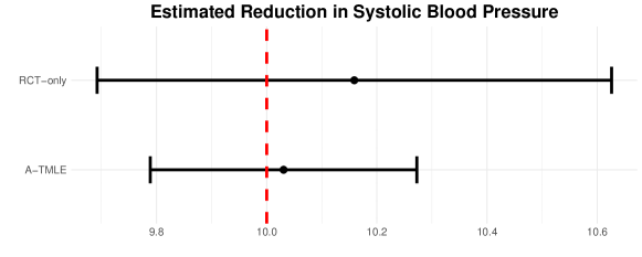
Figure 1: Results for the synthetic data. Point estimates and 95% confidence intervals for the reduction in systolic blood pressure comparing using RCT data only and A-TMLE.

We make the following remarks regarding the algorithm. To estimate nuisance parameters, one might use either highly adaptive lasso (HAL) [23, 24], or super learner [25, 26]. For super learner in particular, one could incorporate a rich library of flexible machine learning algorithms including HAL. Specifically for learning the two working models, we recommend using relaxed-HAL. This approach involves initially fitting a HAL, followed by applying an ordinary least squares regression to the spline basis functions that exhibit non-zero coefficients. Because relaxed-HAL is an MLE, the empirical mean of the $\beta$-component of the canonical gradient is automatically solved. Notably, HAL converges in loss-based dissimilarity at a rate of $n^{-1/3}(\log n)^{2(d-1)/3}$ [27]. Importantly, this rate depends on the dimensionality $d$ only via a power of the $\log n$-factor thus is essentially dimension-free. This allows the learned working model to approximate the truth well. In Appendix D, we also consider several alternative approaches for constructing data-adaptive working models, including learning the working model on independent data sets, and using deep learning architectures to generate dimension reductions of data sets. To complement the methods discussed in Appendix D, we also propose and analyze a cross-validated version of A-TMLE in Appendix C to address concerns regarding potential overfitting of the working models as a result of being too data-adaptive. In addition, as suggested in the Introduction, opting for a slightly larger model than indicated by cross-validation could reduce bias. Techniques like undersmoothing as described in [7] are worth considering. Furthermore, to ensure robustness in model selection, one might enforce a minimal working model based on domain knowledge, specifying essential covariates that must be included. For instance, using HAL to develop the working model could mean exempting certain critical covariates from penalization to guarantee their presence in the final model. This option is available in standard lasso software like the ‘glmnet’ R package [28].

Algorithm 1 has been implemented in the R package ‘atmle’ (available at https://github.com/tq21/atmle). Going back to the synthetic SBP example, we run the implemented algorithm on the simulated data. As we see in Figure 1, the confidence interval produced by A-TMLE is significantly narrower than that obtained from RCT data alone. The red dashed line indicates the true ATE.

7 Asymptotic Super-Efficiency of A-TMLE

In the previous section, we provided detailed steps and strategies for implementing an A-TMLE for our target estimand. In this section, we examine the theoretical properties of A-TMLE. Let $\mathcal{M}_{w,n}=\mathcal{M}_{w,1,n}\times\mathcal{M}_{w,2,n}$. We establish the asymptotic super-efficiency of the A-TMLE $\Psi_{\mathcal{M}_{w,n}}(P_{n}^{*})$ as an estimator of $\Psi(P_{0})$, under specified conditions. This is completely analogue to [6], but is presented to make this article self-contained. It follows the proof of asymptotic efficiency for TMLE applied to $\Psi_{\mathcal{M}_{w,n}}(P_{n}^{*})-\Psi_{\mathcal{M}_{w,n}}(P_{0})$, but with the additional work 1) to deal with the data dependent efficient influence curve in its resulting expansion and 2) to establish that the bias $\Psi_{\mathcal{M}_{w,n}}(P_{0})-\Psi(P_{0})$ is second order. The conditions will be similar to the empirical process and second-order remainder conditions needed for analyzing a TMLE with an additional condition on the data-adaptive working model $\mathcal{M}_{w,n}$ with respect to approximating $P_{0}$.

Let $D_{\mathcal{M}_{w,n},P}$ be the canonical gradient of $\Psi_{\mathcal{M}_{w,n}}$ at $P$. Let $R_{\mathcal{M}_{w,n}}(P,P_{0})\equiv\Psi_{\mathcal{M}_{w,n}}(P)-\Psi_{\mathcal{M}_{w,n}}(P_{0})+P_{0}D_{\mathcal{M}_{w,n},P}$ be the exact remainder. Let $P_{n}^{*}\in{\cal M}_{w,n}$ be an estimator of $P_{0}$ with $P_{n}D_{{\cal M}_{w,n},P_{n}^{*}}=o_{P}(n^{-1/2})$. An MLE over ${\cal M}_{w,n}$ or a TMLE starting with an initial estimator $P_{n}^{0}\in{\cal M}_{w,n}$ targeting $\Psi_{{\cal M}_{w,n}}(P_{0})$ satisfies this efficient score equation condition. Then, by definition of the exact remainder, we have

$$\Psi_{{\cal M}_{w,n}}(P_{n}^{*})-\Psi_{{\cal M}_{w,n}}(P_{0})=(P_{n}-P_{0})D_{{\cal M}_{w,n},P_{n}^{*}}+R_{{\cal M}_{w,n}}(P_{n}^{*},P_{0})+o_{P}(n^{-1/2}).$$

We assume that ${\cal M}_{w,n}$ approximates an oracle model ${\cal M}_{0}$ that contains $P_{0}$ so that

$$\Psi_{{\cal M}_{w,n}}(P_{0})-\Psi(P_{0})=o_{P}(n^{-1/2}).$$

Let $\Psi_{{\cal M}_{0}}(P)=\Psi(\Pi(P\mid{\cal M}_{0}))$, i.e. the projection of $P$ onto $\mathcal{M}_{0}$ applied to $\Psi$. As shown in [6], this does not represent an unreasonable condition. For example, if $P_{0,n}\equiv\Pi(P_{0}\mid{\cal M}_{w,n})\in{\cal M}_{0}$ with probability tending to 1, which holds if ${\cal M}_{w,n}\subset{\cal M}_{0}$, noting that $P_{0}\tilde{D}_{{\cal M}_{w,n},P_{0,n}}=0$ for any $\tilde{D}_{{\cal M}_{w,n},P_{0,n}}$ in the tangent space $T_{{\cal M}_{w,n}}(P_{0,n})$ of the working model at $P_{0,n}$ (due to $P_{0,n}$ be an MLE of $p\rightarrow P_{0}\log p$ over $P\in{\cal M}_{w,n}$). Then, we have

$$\Psi_{{\cal M}_{w,n}}(P_{0})-\Psi(P_{0}) =\Psi(P_{0,n})-\Psi(P_{0})$$

$$=\Psi_{{\cal M}_{0}}(P_{0,n})-\Psi_{{\cal M}_{0}}(P_{0})$$

$$=-P_{0}D_{{\cal M}_{0},P_{0,n}}+R_{{\cal M}_{0}}(P_{0,n},P_{0})$$

$$=(P_{0,n}-P_{0})D_{{\cal M}_{0},P_{0,n}}+R_{{\cal M}_{0}}(P_{0,n},P_{0})$$

$$=(P_{0,n}-P_{0})\left\{D_{{\cal M}_{0},P_{0,n}}-\tilde{D}_{{\cal M}_{w,n},P_{0,n}}\right\}+R_{{\cal M}_{0}}(P_{0,n},P_{0}).$$

The exact remainder $R_{{\cal M}_{0}}(P_{0,n},P_{0})$ is second-order in $p_{0,n}-p_{0}$, so that, if ${\cal M}_{w,n}$ approximates $P_{0}$ at rate $n^{-1/4}$, then this will be $o_{P}(n^{-1/2})$. Regarding the leading term, we can select $\tilde{D}_{{\cal M}_{w,n},P_{0,n}}$ equal to the projection of $D_{{\cal M}_{0},P_{0,n}}$ onto $T_{{\cal M}_{w,n}}(P_{0,n})$ in $L^{2}(P_{0,n})$. Thus, under this condition $\Pi_{{\cal M}_{w,n}}(P_{0})\in{\cal M}_{0}$, using Cauchy-Schwarz inequality, we have that $\Psi_{{\cal M}_{w,n}}(P_{0})-\Psi(P_{0})$ is a second-order difference in two oracle approximation errors $\parallel p_{0,n}-p_{0}\parallel_{\mu}\parallel D_{{\cal M}_{0},P_{0,n}}-\Pi(D_{{\cal M}_{0},P_{0,n}}\mid T_{{\cal M}_{w,n}}(P_{0,n}))\parallel_{\mu}$, where $\mu$ is a dominating measure of $P_{0,n}$ and $P_{0}$. Moreover, one can weaken this condition by defining $\tilde{P}_{0,n}=\Pi(P_{0,n}\mid{\cal M}_{0})$, assuming the above second-order remainder with $P_{0,n}$ replaced by $\tilde{P}_{0,n}$ is $o_{P}(n^{-1/2})$, and assuming that $\Psi(\tilde{P}_{0,n})-\Psi(P_{0,n})=o_{P}(n^{-1/2})$, thereby only assuming that $P_{0,n}$ is close enough to ${\cal M}_{0}$ (instead of being an element of ${\cal M}_{0}$) defined by a distance induced by $\Psi$. So under this reasonable approximation condition on ${\cal M}_{w,n}$ with respect to an oracle model ${\cal M}_{0}$, we have

$$\Psi_{{\cal M}_{w,n}}(P_{n}^{*})-\Psi(P_{0})=(P_{n}-P_{0})D_{{\cal M}_{w,n},P_{n}^{*}}+R_{{\cal M}_{w,n}}(P_{n}^{*},P_{0})+o_{P}(n^{-1/2}).$$

Under the condition that $P_{n}^{*}$ converges to $P_{0}$ at a fast enough rate (i..e, $o_{P}(n^{-1/4})$ so that $R_{{\cal M}_{w,n}}(P_{n}^{*},P_{0})=o_{P}(n^{-1/2})$, this yields

$$\Psi_{{\cal M}_{w,n}}(P_{n}^{*})-\Psi(P_{0})=(P_{n}-P_{0})D_{{\cal M}_{w,n},P_{n}^{*}}+o_{P}(n^{-1/2}).$$

This condition would hold if we use HAL to construct the initial estimator of $P_{0}$ in the TMLE. Under the Donsker class condition that $D_{{\cal M}_{w,n},P_{n}^{*}}$ falls in a $P_{0}$-Donsker class with probability tending to 1, this implies already $\Psi_{{\cal M}_{w,n}}(P_{n}^{*})-\Psi(P_{0})=O_{P}(n^{-1/2})$, consistency at the parametric rate $n^{-1/2}$. Inspection of the canonical gradients for our projection parameters $\Psi_{{\cal M}_{w,n}}$ shows that this is not a stronger condition than the Donsker class condition $D_{\Psi,P_{n}^{*}}$ one would need for the TMLE of $\Psi(P_{0})$. The condition on the working model ${\cal M}_{w,n}$ would hold if the model ${\cal Q}_{w,n}$ falls with probability tending to one in a nice class such as the class of cádlág functions with a universal bound on the sectional variation norm.

Moreover, under the same Donsker class condition, using the consistency of $P_{n}^{*}$, it also follows that

$$\Psi_{{\cal M}_{w,n}}(P_{n}^{*})-\Psi(P_{0})=(P_{n}-P_{0})D_{{\cal M}_{w,n},P_{0}}+o_{P}(n^{-1/2}).$$

Finally, if $D_{{\cal M}_{w,n},P_{0}}$ remains random in the limit but is asymptotically independent of the data $P_{n}$ so that $n^{1/2}P_{n}D_{{\cal M}_{w,n},P_{0}}/\sigma_{0,n}\Rightarrow_{d}N(0,1)$ with $\sigma_{0,n}^{2}\equiv P_{0}D_{{\cal M}_{w,n},P_{0}}^{2}$, then we obtain

$$\sigma_{0,n}^{-1}n^{1/2}\left(\Psi_{{\cal M}_{w,n}}(P_{n}^{*})-\Psi(P_{0})\right)\Rightarrow_{d}N(0,1),$$

thereby allowing for construction of confidence intervals for $\Psi(P_{0})$. If, in fact, $D_{{\cal M}_{w,n},P_{0}}$ converges to a fixed $D_{{\cal M}_{0},P_{0}}$, then we have asymptotic linearity:

$$\Psi_{{\cal M}_{w,n}}(P_{n}^{*})-\Psi(P_{0})=P_{n}D_{{\cal M}_{0},P_{0}}+o_{P}(n^{-1/2}),$$

with influence curve the efficient influence curve of $\Psi_{{\cal M}_{0}}:{\cal M}\rightarrow\hbox{${\rm I\kern-1.99997ptR}$}$ at $P_{0}$. Moreover, [6] shows that $D_{{\cal M}_{0},P_{0}}$ equals the efficient influence curve of $\Psi:{\cal M}_{0}\rightarrow\hbox{${\rm I\kern-1.99997ptR}$}$ that a priori assumes the model ${\cal M}_{0}$, showing that this adaptive-TMLE is super-efficient achieving the efficiency bound for estimation $\Psi(P_{0})$ under the oracle model ${\cal M}_{0}$ (as if we are given $P_{0}\in{\cal M}_{0}$ for given ${\cal M}_{0}$).

Thus, if the true $\tau_{P_{0}}$ is captured by a small model, then the adaptive-TMLE will achieve a large gain in efficiency relative to the regular TMLE, while if $\tau_{P_{0}}$ is complex so that ${\cal M}_{0}$ is close to ${\cal M}$, then the gain in efficiency will be small or the adaptive-TMLE will just be asymptotically efficient. The discussions above are summarized into the following theorem.

Theorem 1.

Let $D_{{\cal M}_{w,n},P}$ be the canonical gradient of $\Psi_{{\cal M}_{w,n}}=\Psi(\Pi(\cdot\mid{\cal M}_{w,n}))$ at $P$. Let $R_{{\cal M}_{w,n}}(P,P_{0})\equiv\Psi_{{\cal M}_{w,n}}(P)-\Psi_{{\cal M}_{w,n}}(P_{0})+P_{0}D_{{\cal M}_{w,n},P}$ be the exact remainder. Let ${\cal M}_{0}\subset{\cal M}$ contain $P_{0}$, a so-called oracle model, and $D_{{\cal M}_{0},P}$ and $R_{{\cal M}_{0}}(P,P_{0})$ be the canonical gradient and exact remainder of $\Psi_{{\cal M}_{0}}:{\cal M}\rightarrow\hbox{${\rm I\kern-1.99997ptR}$}$, respectively. Let $P_{n}^{*}\in{\cal M}_{w,n}$ be an estimator of $P_{0}$ such that $P_{n}D_{{\cal M}_{w,n},P_{n}^{*}}=o_{P}(n^{-1/2})$. Then,

$$\Psi_{{\cal M}_{w,n}}(P_{n}^{*})-\Psi_{{\cal M}_{w,n}}(P_{0})=(P_{n}-P_{0})D_{{\cal M}_{w,n},P_{n}^{*}}+R_{{\cal M}_{w,n}}(P_{n}^{*},P_{0}).$$

Oracle model approximation condition: Let $P_{0,n}\equiv\Pi_{{\cal M}_{w,n}}(P_{0})$ and $\tilde{P}_{0,n}=\Pi(P_{0,n}\mid{\cal M}_{0})$. Let $\tilde{D}_{{\cal M}_{w,n},P_{0,n}}$ be the projection of $D_{{\cal M}_{0},P_{0,n}}$ onto the tangent space $T_{{\cal M}_{w,n}}(P_{0,n})\subset L^{2}_{0}(P_{0,n})$ of the working model ${\cal M}_{w,n}$ at $P_{0,n}$. Assume that ${\cal M}_{w,n}$ approximates ${\cal M}_{0}$ in the sense that $\Psi(\tilde{P}_{0,n})-\Psi(P_{0,n})=o_{P}(n^{-1/2})$ and

$$(\tilde{P}_{0,n}-P_{0})\left\{D_{{\cal M}_{0},\tilde{P}_{0,n}}-\tilde{D}_{{\cal M}_{w,n},\tilde{P}_{0,n}}\right\}=o_{P}(n^{-1/2}).$$

Then, we have

$$\Psi_{{\cal M}_{w,n}}(P_{n}^{*})-\Psi(P_{0})=(P_{n}-P_{0})D_{{\cal M}_{w,n},P_{n}^{*}}+R_{{\cal M}_{w,n}}(P_{n}^{*},P_{0})+o_{P}(n^{-1/2}).$$

Rate of convergence condition: Under the condition that $P_{n}^{*}$ converges to $P_{0}$ at a fast enough rate (i.e., $o_{P}(n^{-1/4})$ so that $R_{{\cal M}_{w,n}}(P_{n}^{*},P_{0})=o_{P}(n^{-1/2})$, this yields

$$\Psi_{{\cal M}_{w,n}}(P_{n}^{*})-\Psi(P_{0})=(P_{n}-P_{0})D_{{\cal M}_{w,n},P_{n}^{*}}+o_{P}(n^{-1/2}).$$

Donsker class condition: Under the Donsker class condition that $D_{{\cal M}_{w,n},P_{n}^{*}}$ falls in a $P_{0}$-Donsker class with probability tending to 1, this implies $\Psi_{{\cal M}_{w,n}}(P_{n}^{*})-\Psi(P_{0})=O_{P}(n^{-1/2})$, consistency at the parametric rate $n^{-1/2}$. Moreover, under the same Donsker class condition, using the consistency $P_{0}\{D_{{\cal M}_{w,n},P_{n}^{*}}-D_{{\cal M}_{w,n},P_{0}}\}^{2}\rightarrow_{p}0$ of $P_{n}^{*}$, it also follows that

$$\Psi_{{\cal M}_{w,n}}(P_{n}^{*})-\Psi(P_{0})=(P_{n}-P_{0})D_{{\cal M}_{w,n},P_{0}}+o_{P}(n^{-1/2}).$$

Asymptotic normality condition: Finally, if $D_{{\cal M}_{w,n},P_{0}}$ remains random in the limit but is asymptotically independent of the data $P_{n}$ in the sense that $n^{1/2}P_{n}D_{{\cal M}_{w,n},P_{0}}/\sigma_{0,n}\Rightarrow_{d}N(0,1)$ with $\sigma_{0,n}^{2}\equiv P_{0}D_{{\cal M}_{w,n},P_{0}}^{2}$, then we obtain

$$\sigma_{0,n}^{-1}n^{1/2}\left(\Psi_{{\cal M}_{w,n}}(P_{n}^{*})-\Psi(P_{0})\right)\Rightarrow_{d}N(0,1),$$

thereby allowing for construction of confidence intervals for $\Psi(P_{0})$. If, in fact, $D_{{\cal M}_{w,n},P_{0}}$ converges to a fixed $D_{{\cal M}_{0},P_{0}}$, then we have asymptotic linearity:

$$\Psi_{{\cal M}_{w,n}}(P_{n}^{*})-\Psi(P_{0})=P_{n}D_{{\cal M}_{0},P_{0}}+o_{P}(n^{-1/2}),$$

with influence curve the efficient influence curve of $\Psi_{{\cal M}_{0}}:{\cal M}\rightarrow\hbox{${\rm I\kern-1.99997ptR}$}$ at $P_{0}$. Moreover, $D_{{\cal M}_{0},P_{0}}$ equals the efficient influence curve of $\Psi:{\cal M}_{0}\rightarrow\hbox{${\rm I\kern-1.99997ptR}$}$ that a priori assumes the model ${\cal M}_{0}$.

8 Simulation Studies

We conducted two sets of simulations to evaluate our A-TMLE estimator against alternative methods. The first simulation setting involves augmenting both the treatment and control arm. The second simulation is a scenario with rare binary outcomes using only control data from the real-world, a situation likely when treatment data are unavailable, for example, due to pending drug approvals and the rarity of the outcome could lead to an underpowered RCT. Additional simulations for more general data structures with missing outcomes are available in Appendix B. Descriptions of the five estimators we assessed is shown in Table 1.

Table 1: Estimators assessed in simulation studies and their descriptions.

Estimator	Description
A-TMLE	Our proposed estimator, applying the A-TMLE framework to estimate both the pooled-ATE $\tilde{\Psi}$ and the bias $\Psi^{\#}$.
ES-CVTMLE	An estimator for integrating RCT with RWD within the TMLE framework, data-adaptively chooses between RCT-only or pooled-ATE to optimize bias-variance trade-off [16].
PROCOVA	A prognostic score covariate-adjustment method [22].
TMLE	A standard TMLE for the target parameter.
RCT-only	A standard TMLE for ATE parameter using RCT data alone, serving as the best estimator in the absence of external data.

Our primary metrics for evaluating the performance of the estimators include mean-squared-error (MSE), relative MSE, coverage and width of 95% confidence intervals.

8.1 Augmenting both the treatment and control arm

Scenarios (a) and (b) have bias functions (specifically, the conditional effect of the study indicator on the outcome) of simple main-term linear forms, while in scenarios (c) and (d) we introduced complex biases involving indicator jumps, higher-order polynomial terms and interactions, demonstrating the misspecification of a main-term linear model and the necessity of employing HAL as a flexible nonparametric regression algorithm for accurate approximation of the bias function. In scenarios (a) and (b), we constructed a hybrid design with the external data sample size being threefold that of the RCT, mirroring the common scenario where, for example, electronic health records databases offer a substantially larger pool of external data. The external dataset comprises both treated and control patients. In the RCT, the probability of assignment to the active treatment group is 0.67, reflecting realistic scenarios where a drug has been approved and the focus is on assessing safety for secondary outcomes. Treatment assignment in the external data mimics real-world conditions, determined by baseline patient characteristics, as would be the case in clinical practice. To ensure that a straightforward pooling of the two data sources would yield a biased estimate of the true ATE, we added a bias term to the outcome of the patients from the external data.

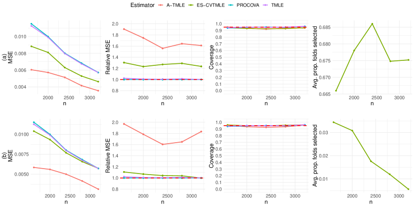
Figure 2: Comparing the MSE, relative MSE, 95% confidence interval coverage of A-TMLE, ES-CVTMLE, and TMLE estimator for increasing sample sizes of both the RCT and external data. The reference (red dashed line) in the relative MSE plots are the MSEs of the RCT-only estimator. The plots in the right-most column show the average proportion of cross-validation folds the ES-CVTMLE estimator pooled the external data.

Figure 2 demonstrates that the A-TMLE estimator (red line) has significantly lower MSE than both ES-CVTMLE and TMLE across scenarios (a) and (b), being 1.5 times more efficient than an efficient estimator that uses RCT data alone. All estimators maintain nominal 95% confidence interval coverage. Notice that, in scenario (a), the smaller bias from external data allows ES-CVTMLE (green line) to achieve moderate efficiency gains over TMLE (blue line), with the pooled parameter selected in about 70% of its cross-validation folds, indicating its ability to utilize external data for efficiency improvements. Despite this, A-TMLE surpasses ES-CVTMLE in efficiency gains. Scenario (b) amplifies the bias magnitude introduced from the external data, severely diminishing ES-CVTMLE’s efficiency gain, nearly to nonexistence asymptotically. Conversely, A-TMLE’s capability to accurately learn the bias working model data-adaptively enhances its efficiency significantly, even as the sample size increases and despite the larger bias, maintaining robust type 1 error control. ES-CVTMLE’s failure to achieve efficiency gain in scenario (b) is highlighted by its near-total rejection of the external data due to large estimated bias. Recall that in the Introduction section, we mentioned that an efficient estimator for the target parameter $\Psi$ may still offer no gain in the presence of external data, this point is demonstrated in the relative MSE plots with an efficient TMLE that goes after $\Psi$ (blue line) matching the MSE of an estimator using RCT data only (red dashed line). Therefore, even theoretically optimal estimators may not yield efficiency gains from external data integration.

In some practical settings, bias may deviate from the simple main-term linear model we considered in our first simulation, manifesting as a complex function of baseline covariates and treatment. This complexity necessitates the employment of more flexible nonparametric learning algorithms for accurate bias estimation. Hence, our second simulation utilizes HAL with a rich set of spline basis functions to data-adaptively learn the bias working model. Echoing the design of the first simulation, we increase the external data’s sample size to five times that of the RCT, maintaining a 0.67 treatment randomization probability within the RCT, and both treated and control patients are present in the external data. The bias term in this scenario includes indicator jumps, higher-order polynomials, and interaction terms, rendering a simple main-term linear model misspecified. The data-generating process is provided in Appendix B.

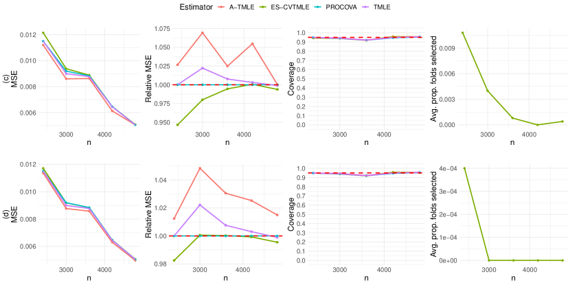
Figure 3: Comparing the MSE, relative MSE, 95% confidence interval coverage of A-TMLE, ES-CVTMLE, and TMLE estimator for increasing sample sizes of both the RCT and external data. The reference (red dashed line) in the relative MSE plots are the MSEs of the RCT-only estimator. The plots in the right-most column show the average proportion of cross-validation folds the ES-CVTMLE estimator pooled the external data.

Figure 3 shows that in scenarios with complex bias, ES-CVTMLE fails to achieve any efficiency gain, and at times, it underperforms by having a higher MSE compared to that of a TMLE on the RCT data alone. This may stem from not estimating the bias accurately or as a result of its cross-validation method not fully leveraging the data due to the requirements for bias and variance estimation for the selection criteria. Conversely, A-TMLE continues to secure a notable efficiency gain while maintaining valid type 1 error control. Table 2 shows the average width of confidence interval lengths across varying sample sizes and simulation runs of A-TMLE as a percentage of that of other methods. In scenarios (a) and (b), the confidence intervals produced by A-TMLE are much smaller. For scenarios (c) and (d), the reduction in widths is smaller, but still superior compared with competitors.

Table 2: A-TMLE’s 95% CI width as a percentage of other methods’.

Method	Scenario (a)	Scenario (b)	Scenario (c)	Scenario (d)
ES-CVTMLE	66.1%	60.4%	98.3%	98.2%
Regular TMLE	59.1%	61.2%	99.1%	99.1%
PROCOVA	59.0%	61.1%	99.0%	99.0%
RCT-only	59.0%	61.1%	99.0%	99.0%

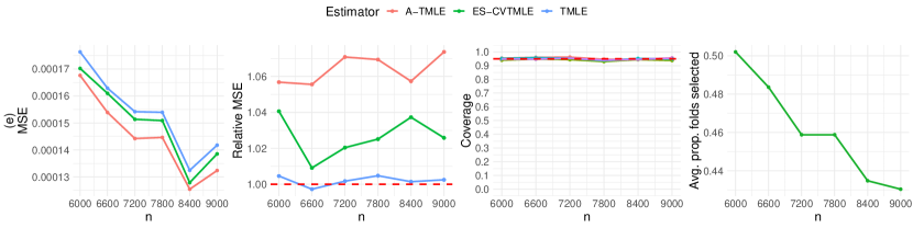
Figure 4: Comparing the MSE, relative MSE, 95% confidence interval coverage of A-TMLE, ES-CVTMLE, and TMLE estimator for increasing sample sizes of both the RCT and external data. The reference (dashed red line) in the relative MSE plots are the MSEs of the RCT-only estimator. The plots in the right-most column show the average proportion of cross-validation folds the ES-CVTMLE estimator pooled the external data.

8.2 Augmenting using only external control subjects

In the second simulation study, we focus on a scenario with a rare binary outcome, augmenting only external controls. The incidence rate of this outcome ranges from 5% to 8% in the pooled data. Details of the data-generating process are provided in Appendix B. The results, displayed in Figure 4, indicate that A-TMLE remains the optimal choice.

9 Discussion

In this article, we introduced adaptive-TMLE for the estimation of the average treatment effect using combined data from randomized controlled trials and real-world data. The target parameter is conservatively designed to fully respect the RCT as the gold standard for treatment effect estimation without requiring additional identification assumptions beyond those inherent to RCTs. The only extra requirement is that every individual in the combined dataset must have a non-zero probability of trial enrollment, a condition typically ensured during the sampling phase for external patients. Despite focusing on a conservative target parameter where an efficient estimator might still lack power, our proposed A-TMLE demonstrated potential efficiency gains. These gains are primarily driven by the complexity of the bias working model rather than its magnitude, which is crucial as the bias might be simple yet substantial. The working model for the bias and pooled-ATE estimand are data-adaptively learned, which may be much smaller than the nonparametric model, thus allowing efficiency gain. Importantly, since we do not impose extra assumptions, virtually any external data, even those with a different outcome from the RCT, could be utilized. This approach could extend to scenarios involving surrogate outcomes, where the difference in the outcomes might be adequately approximated as a function of covariates and treatment. Additionally, A-TMLE could be useful when researchers have access to a well-designed observational study for identifying the desired causal effect, alongside other observational data potentially subject to unmeasured confounding. In these cases, combining data sources could yield a more accurate estimator of the causal effect. Extending this approach to handle multiple external data sources could be achieved either by stratifying based on the study to learn a separate bias function for each, or by pooling across studies to jointly learn a bias function. One limitation of A-TMLE is that, although theoretically the efficiency gain is driven by the complexity of the bias working model, it remains unclear in practice how much efficiency gain one should expect. For instance, our simulations have shown situations where A-TMLE is almost twice as efficient, yet other cases where the efficiency gain is small, although still better than alternative approaches. Future research should explore how much efficiency gain one can expect in finite samples. Another limitation is the challenge of determining how to enforce a minimal working model without compromising efficiency gains. Without such a minimal working model, one runs the risk of introducing bias if cross-validation overly favors a sparse model when the true model is actually complex. A better understanding of this trade-off is necessary to provide concrete guidelines on the minimal working model.

Appendix A: Proof of Lemmas

Proof of lemma 1.

First consider the case that we do not assume $S\perp W$ but possibly have a model on $g(A\mid S,W)$. Then the efficiency bound corresponds with the one in the nonparametric model due to the target parameter only depending on $P_{W}$ and $\bar{Q}$, and that the tangent space of $g$ is orthogonal to the tangent space of these nuisance parameters. Therefore, it suffices to derive the influence curve of the empirical plug-in estimator acting as if $W$ is discrete, which then also establishes the general efficient influence curve by an approximation argument. The influence curve of the empirical plug-in estimator $\Psi(P_{n})$ is straightforward to derive by using that the canonical gradient/influence curve of the empirical estimate of $E(Y\mid W=w,A=a,S=s)$ is given by $E(Y\mid W=w,A=a,S=1)=I(S=1,A=a,W=w)/p(S=1,W=w,A=a)(Y-\bar{Q}(S,W,A))$, while we use the empirical measure of $W_{1},\ldots,W_{n}$ as estimator of $P_{W}$. Consider now the statistical model that also assumes that $S\perp W$. The only way this model assumption can affect the estimator is that it might yield a different estimator of $P_{W}$ than the empirical measure. However, the empirical distribution of $W$ is still an efficient estimator of $P_{W}$, even when $S$ is independent of $W$. In other words, if we have two samples of $W$ from the same population, then the efficient estimator of the marginal distribution of $W$ is still the empirical measure of the combined sample on $W$. The proof for $\Psi_{2}$ is similar. If we assume $S\perp W$, then the canonical gradient for $\Psi_{2}$ changes a little due to an efficient estimator of $P_{W\mid S=1}$ should now use the empirical measure of $W$ for the combined sample, instead of using the empirical measure of $W$, given $S=1$. ∎

Proof of lemma 3.

The proof is analogous to the proof of Lemma 6 by replacing $A$ with $S$. Specifically, in Lemma 6, we show the loss function for learning the working model for the conditional effect of $A$ on $Y$. Here, in Lemma 3, we have a similar loss function for learning the conditional effect of $S$ on $Y$. ∎

Proof of lemma 4.

The proof is analogous to the proof of Lemma 7 by replacing $A$ with $S$ and $W$ with $W,A$. ∎

Proof of lemma 5.

The $p_{Y\mid S,W,A}$-score component of $D_{{\cal M}_{w,2},P}^{\#}$ is given by

$$D_{{\cal M}_{w,2},\beta,P}^{\#} \equiv\left\{E_{P}\Pi_{P}(0\mid W,0)\frac{d}{d\beta(P)}\tau_{w,\beta(P)}(W,0)\right\}^{\top}D_{\beta,P}(O)$$

$$-\left\{E_{P}\Pi_{P}(0\mid W,1)\frac{d}{d\beta(P)}\tau_{w,\beta(P)}(W,1)\right\}^{\top}D_{\beta,P}(O)$$

$$=\sum_{j}D_{\beta,P,j}E_{P}\Pi_{P}(0\mid W,0)\phi_{j}(W,0)-\sum_{j}D_{\beta,P,j}E_{P}\Pi_{P}(0\mid W,1)\phi_{j}(W,1).$$

The $p_{W}$-score component of $D_{{\cal M}_{w,2},W,P}^{\#}$ is given by

$$D^{\#}_{{\cal M}_{w,2},W,P}\equiv\Pi_{P}(W,0)\tau_{w,\beta(P)}(W,0)-\Pi_{P}(W,1)\tau_{w,\beta(P)}(W,1)-\Psi_{{\cal M}_{w,2}}^{\#}(P).$$

Finally we need the contribution from the dependence of $\Psi^{\#}_{{\cal M}_{w,2}}(P)$ on the conditional distribution $\Pi_{P}$. The influence curve of $\Pi_{P}(0\mid w,a)$ is given by $D_{{\cal M}_{w},\Pi_{P},(w,a),P}=I(W=w,A=a)/P(w,a)(I(S=0)-\Pi_{P}(0\mid w,a))$. So $\Pi_{P}$-score component of $D_{{\cal M}_{w,2},P}^{\#}$ is given by

$$D^{\#}_{{\cal M}_{w},\Pi_{P},P} \equiv\int_{w}I(W=w,A=0)/P(w,0)\tau_{w,\beta(P)}(w,0)(I(S=0)-\Pi_{P}(0\mid W,0))dP(w)$$

$$-\int_{w}I(W=w,A=1)/P(w,1)\tau_{w,\beta(P)}(w,1)(I(S=0)-\Pi_{P}(0\mid W,1))dP(w)$$

$$=\left\{\frac{I(A=0)}{g_{P}(0\mid W)}\tau_{w,\beta(P)}(W,0)-\frac{I(A=1)}{g_{P}(1\mid W)}\tau_{w,\beta(P)}(W,1)\right\}(I(S=0)-\Pi_{P}(0\mid W,A)).$$

Now note that $I(S=0)-\Pi(0\mid W,A)=-(I(S=1)-\Pi(1\mid W,A))$. Therefore, we have

$$D^{\#}_{{\cal M}_{w},\Pi_{P},P}=\left\{\frac{A}{g_{P}(1\mid W)}\tau_{w,\beta(P)}(W,0)-\frac{1-A}{g_{P}(0\mid W)}\tau_{w,\beta(P)}(W,1)\right\}(S-\Pi_{P}(1\mid W,A)).$$

So, we have every component in

$$D^{\#}_{{\cal M}_{w,2},P}=D^{\#}_{{\cal M}_{w,2},W,P}+D^{\#}_{{\cal M}_{w,2},\Pi,P}+D^{\#}_{{\cal M}_{w,2},\beta,P}.$$

∎

Proof of lemma 6.

We have $\bar{Q}^{r}_{P}=\theta(P)+AT_{P}$, where $\theta(P)=E_{P}(Y\mid A=0,W)$ and $T_{P}=E_{P}(Y\mid A=1,W)-E_{P}(Y\mid A=0,W)$. We have to compute a projection of $\bar{Q}^{r}_{P}$ onto the linear space $\theta(W)+A\sum_{j}\beta(j)\phi_{j}$. We can write

$$\theta(W)+A\sum_{j}\beta(j)\phi_{j}=\left(\theta(W)+g(W)\sum_{j}\beta_{j}\phi_{j}\right)+(A-g(W))\sum_{j}\beta(j)\phi_{j}.$$

Thus, the linear space on which we are projecting is an orthogonal sum of $L^{2}(P_{W})$ and the linear span of $\{(A-g(W))\phi_{j}:j\}$. In $L^{2}(P)$, functions of $W$ are orthogonal to the linear span of $\{(A-g(W))\phi_{j}:j\}$. Therefore the projection of $\bar{Q}_{P}$ on this orthogonal sum space is given by $E(\bar{Q}_{P}\mid W)=E_{P}(Y\mid W)$ plus the projection of $\bar{Q}_{P}=\theta(P)+AT_{P}$ onto $\{(A-g(W))\phi_{j}:j\}$. The projection of $\theta(P)$ on this linear span equals zero since a function of $W$ is orthogonal to $(A-g(W))\phi_{j}$. The projection of $AT_{P}$ is given by $(A-g(W))\sum_{j}\beta_{P}(j)\phi_{j}$ with $\beta(P)=\arg\min_{\beta}E_{P}(AT_{P}(W)-(A-g(W))\sum_{j}\beta_{j}\phi_{j}(W))^{2}$. We can write $AT_{P}=(A-g(W))T_{P}(W)+g(W)T_{P}(W)$. So $\beta(P)=\arg\min_{\beta}E_{P}(A-g(W))^{2}(T_{P}(W)-\sum_{j}\beta_{j}\phi_{j}(W))^{2}$, which equals $\arg\min_{\beta}E_{P}g_{P}(1-g_{P})(W)(T_{P}(W)-\sum_{j}\beta_{j}\phi_{j}(W))^{2}$. This proves the lemma. ∎

Proof of lemma 7.

We want to derive the canonical gradient of $\beta(P)$ defined on a nonparametric model. Our starting point is that

$$\beta(P)=\arg\min_{\beta}E_{P}\left(Y-(A-g_{P}(W))\sum_{j}\beta_{j}\phi_{j}(W)\right)^{2}.$$

This shows that $\beta(P)$ solves the equation

$$U(P,g_{P},\beta)=E_{P}(A-g_{P}(W)){\bf\phi}(W)\left(Y-(A-g_{P}(W))\sum_{j}\beta(j)\phi_{j}\right)=0.$$

By the implicit function theorem, for paths $\{P_{\epsilon}:\epsilon\}$ through $P$ at $\epsilon=0$, we have at $\epsilon=0$:

$$\frac{d}{d\epsilon}\beta(P_{\epsilon})=-\frac{d}{d\beta}U(P,g,\beta)^{-1}\frac{d}{d\epsilon}U(\beta(P),P_{\epsilon},g_{\epsilon}).$$

Let $I_{P}=E_{P}g(1-g)(W){\bf\phi}{\bf\phi}^{\top}$, then it follows that

$$D_{\beta,P}=I_{P}^{-1}\{D_{1,P}+D_{2,P}\},$$

where $D_{1,P}$ is the canonical gradient of $P\rightarrow U(\beta_{1},P,g_{1})$ at $\beta_{1}=\beta(P)$ and $g_{1}=g_{P}$, and $D_{2,P}$ is the canonical gradient of $P\rightarrow U(\beta_{1},P_{1},g_{P})$ at $\beta_{1}=\beta(P)$ and $P_{1}=P$. Since $U(\beta_{1},P,g_{1})$ is just a mean parameter with respect to $P$ (like $E_{P}D$ which has canonical gradient $D-E_{P}D$), it follows that

$$D_{1,P}=(A-g_{P}(W)){\bf\phi}(W)\left(Y-(A-g_{P}(W))\sum_{j}\beta_{P}(j)\phi_{j}(W)\right).$$

Moreover,

$$U(\beta_{1},P_{1},g_{P})=E_{P_{1}}(A-g_{P}(W)){\bf\phi}(W)\left(\bar{Q}_{P_{1}}-(A-g_{P}(W))\sum_{j}\beta_{P_{1}}(j)\phi_{j}\right).$$

Therefore, it remains to determine the canonical gradient of

$$P \rightarrow\int_{w,a}p_{1}(w,a)(a-g_{P}(w)){\bf\phi}(w)(\bar{Q}_{1}(w,a)-(a-g_{P}(w))\sum_{j}\beta_{1}(j)\phi_{j}(w))d\mu(w,a)$$

$$=\int_{w,a}p_{1}(w,a)(a-g_{P}(w)){\bf\phi}(w)\bar{Q}_{1}(w,a)-\int_{w,a}p_{1}(w,a)(a-g_{P}(w))^{2}{\bf\phi}(w)\sum_{j}\beta_{1}(j)\phi_{j}(w)$$

at $p_{1}=p$. We know that the canonical gradient of $P\rightarrow g_{P}(w)$ is given by $I(W=w)/p(w)(A-g_{P}(W))$. So, by the delta-method, the canonical gradient is given by

$$D_{2,P}(W,A) =-\int_{w,a}p(w)g(a\mid w)I(W=w)/p(w)(A-g_{P}(W)){\bf\phi}(w)\bar{Q}_{P}(w,a)d\mu(w,a)$$

$$+2\int_{w,a}p(w)g(a\mid w)(a-g_{P}(w)){\bf\phi}(w)I(W=w)/p(w)(A-g_{P}(W))\sum_{j}\beta(j)\phi_{j}(w)d\mu(w,a)$$

$$=-(A-g_{P}(W)){\bf\phi}(W)\int_{a}g(a\mid W)\bar{Q}_{P}(W,a)d\mu(a\mid w)$$

$$+2(A-g_{P}(W)){\bf\phi}(W)\sum_{j}\beta(j)\phi_{j}(W)\int_{a}g(a\mid W)(a-g_{P}(W))d\mu(a\mid w)$$

$$=-(A-g_{P}(W)){\bf\phi}(W)\tilde{\theta}_{P}(W),$$

since $\int_{a}g_{P}(a\mid W)(a-g_{P}(W))d\mu(a\mid w)=E_{P}(A-E_{P}(A\mid W))=0$. Thus,

$$D_{1,P}+D_{2,P} =(A-g_{P}(W)){\bf\phi}(W)\left(Y-(A-g_{P}(W))\sum_{j}\beta_{P}(j)\phi_{j}(W)\right)-(A-g_{P}(W)){\bf\phi}(W)\tilde{\theta}_{P}(W)$$

$$=(A-g_{P}(W)){\bf\phi}(W)\left(Y-\tilde{\theta}_{P}(W)-(A-g_{P}(W))\sum_{j}\beta_{P}(j)\phi_{j}(W)\right).$$

This proves that

$$D_{\beta,P}^{r}=I_{P}^{-1}(A-g_{P}(W)){\bf\phi}(W)(Y-\tilde{\theta}_{P}^{r}(W)-(A-g_{P}(W))\sum_{j}\beta_{P}(j)\phi_{j}(W)),$$

where $I_{P}=E_{P}g(1-g)(W){\bf\phi}{\bf\phi}^{\top}$. ∎

Appendix B: Data-Generating Processes, Missing Outcome Data Structure and Simulations

The data-generating process for the SBP synthetic study in Section 6 is:

$$U_{Y} \sim\mathcal{N}(0,1)$$

$$\text{Age}=W_{1} \sim\mathcal{N}(50,12^{2})$$

$$\text{BMI}=W_{2} \sim\mathcal{N}(28,5^{2})$$

$$\text{Smoking}=W_{3} \sim\text{Bern}(0.2)$$

$$\text{Health literacy}=W_{4} \sim\mathcal{N}(50,10^{2})\text{ (unmeasured)}$$

$$\text{SES}=W_{5} \sim\mathcal{N}(50,10^{2})\text{ (unmeasured)}$$

$$A \sim\left\{\begin{array}[]{ll}\text{Bern}(0.5)&\text{if }S=1\\ \text{Bern}(\text{expit}(-1.5+0.05W_{1}+0.04W_{2}+0.8W_{3}+0.03W_{4}+0.02W_{5}))&\text{if }S=0\end{array}\right.$$

$$Y =120-0.1W_{1}+0.05W_{2}^{2}-5W_{3}+0.04W_{4}+0.03W_{5}+U_{Y}.$$

The data-generating process for scenarios (a) and (b) in Section 8 is:

$$U_{Y} \sim\mathcal{N}(0,1)$$

$$W_{1} \sim\mathcal{N}(0,1)$$

$$W_{2} \sim\mathcal{N}(0,1)$$

$$W_{3} \sim\mathcal{N}(0,1)$$

$$A \sim\left\{\begin{array}[]{ll}\text{Bern}(0.67)&\text{if }S=1\\ \text{Bern}(\text{expit}(0.5W_{1}))&\text{if }S=0\end{array}\right.$$

$$B =\left\{\begin{array}[]{ll}0.2+0.1W_{1}\cdot I(A=0)&\text{scenario (a)}\\ 0.5+3.1W_{1}\cdot I(A=0)+0.8W_{3}&\text{scenario (b)}\end{array}\right.$$

$$Y =2.5+0.9W_{1}+1.1W_{2}+2.7W_{3}+1.5A+U_{Y}+I(S=0)\cdot B.$$

The data-generating process for scenarios (c) and (d) in Section 8 is:

$$U_{Y} \sim\mathcal{N}(0,1)$$

$$W_{1} \sim\text{Uniform}(0,1)$$

$$W_{2} \sim\text{Uniform}(0,1)$$

$$W_{3} \sim\text{Uniform}(0,1)$$

$$A \sim\left\{\begin{array}[]{ll}\text{Bern}(0.67)&\text{if }S=1\\ \text{Bern}(\text{expit}(W_{1}))&\text{if }S=0\end{array}\right.$$

$$B =\left\{\begin{array}[]{ll}0.3+0.9W_{2}\cdot I(A=0)+0.7W_{3}\cdot I(W_{2}>0.5)&\text{scenario (c)}\\ 0.3+1.1W_{1}\cdot I(A=0)+0.9W_{2}^{2}W_{3}&\text{scenario (d)}\end{array}\right.$$

$$Y =1.9+4.2A+0.9W_{1}+1.4W_{2}+2.1W_{3}+U_{Y}+I(S=0)\cdot B.$$

The data-generating process for scenario (e) in Section 8 is:

$$U_{Y} \sim\mathcal{N}(0,1)$$

$$W_{1} \sim\text{Uniform}(0,1)$$

$$W_{2} \sim\text{Uniform}(0,1)$$

$$W_{3} \sim\text{Bern}(0.5)$$

$$A \sim\text{Bern}(0.67)$$

$$B =0.2+0.1W_{1}\cdot I(A=0)$$

$$Y \sim\text{Bern}(\text{expit}(-3-0.9W_{1}+0.5W_{2}-0.7W_{3}+0.9A+I(S=0)\cdot B)).$$

When the outcome is subject to missingness, we consider the more general missing data structure $O=(S,W,A,\Delta,\Delta\cdot Y)$ where $\Delta$ is an indicator that equals to one if the outcome is observed. In this case, we consider the target parameter given by

$$\Psi(P)=\mathbb{E}_{W}\mathbb{E}(Y_{1}-Y_{0}\mid S=1,W,\Delta=1).$$

In other words, we are interested in the causal effect in the world where everyone’s outcome is available. The identification of this target parameter requires an additional coarsening at random (or missing at random) assumption, which states that $(Y_{1},Y_{0})\perp\Delta\mid W,S=1$. Together with assumptions A1, A2 and A3 from Section 2, we have the target estimand given by

$$\Psi(P_{0})=\mathbb{E}_{0}[\mathbb{E}_{0}(Y\mid S=1,W,A=1,\Delta=1)-\mathbb{E}_{0}(Y\mid S=1,W,A=0,\Delta=1)].$$

Now, to learn the working models for the effect of $S$ on $Y$ and the effect of $A$ on $Y$, we use the following two loss functions, respectively:

$$L_{\tilde{\theta}_{P},\Pi_{P},g^{\Delta}_{P}}(\tau) =\frac{\Delta}{g^{\Delta}_{P}(1\mid S,W,A)}\left(Y-\tilde{\theta}_{P}(W,A)-(S-\Pi_{P}(1\mid W,A))\tau\right)^{2},$$

$$L_{\tilde{\theta}^{r}_{P},g_{P},\tilde{g}^{\Delta}_{P}}(T) =\frac{\Delta}{\tilde{g}^{\Delta}_{P}(1\mid W,A)}(Y-\tilde{\theta}^{r}_{P}(W)-(A-g_{P}(1\mid W))T(W))^{2},$$

where $g^{\Delta}_{P}(1\mid S,W,A)\equiv P(\Delta=1\mid S,W,A)$ and $\tilde{g}^{\Delta}_{P}(1\mid W,A)\equiv P(\Delta=1\mid W,A)$. In addition, we also multiply the factor $\Delta/g^{\Delta}_{P}(1\mid S,W,A)$ and $\Delta/\tilde{g}^{\Delta}_{P}(1\mid W,A)$ to the $Y$-components of the canonical gradients of the projection parameters we showed in Lemma 5 and 8 respectively. We conducted simulations for the scenario where outcome is subject to missingness. The data-generating process is:

$$U_{Y} \sim\mathcal{N}(0,1)$$

$$W_{1} \sim\mathcal{N}(0,1)$$

$$W_{2} \sim\mathcal{N}(0,1)$$

$$W_{3} \sim\mathcal{N}(0,1)$$

$$A \sim\left\{\begin{array}[]{ll}\text{Bern}(0.67)&\text{if }S=1\\ \text{Bern}(\text{expit}(0.5W_{1}))&\text{if }S=0\end{array}\right.$$

$$B =\left\{\begin{array}[]{ll}0.2+0.1W_{1}\cdot I(A=0)&\text{scenario (a)}\\ 0.5+3.1W_{1}\cdot I(A=0)+0.8W_{3}&\text{scenario (b)}\end{array}\right.$$

$$\Delta =\text{Bern}(\text{expit}(2.3+0.8W_{1}))$$

$$Y =\Delta[2.5+0.9W_{1}+1.1W_{2}+2.7W_{3}+1.5A+U_{Y}+I(S=0)\cdot B].$$

See figure 5 for results.

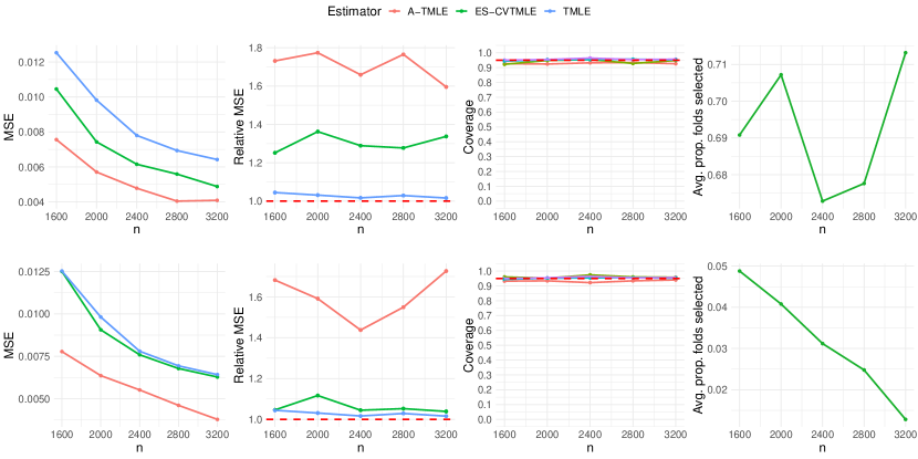
Figure 5: Comparing the MSE, relative MSE, 95% confidence interval coverage of A-TMLE, ES-CVTMLE, and TMLE estimator for increasing sample sizes of both the RCT and external data. The reference (dashed red line) in the relative MSE plots are the MSEs of the RCT-only estimator. The plots in the right-most column show the average proportion of cross-validation folds the ES-CVTMLE estimator pooled the external data.

Appendix C: Adaptive CV-TMLE

The A-TMLE is targeting a data dependent target parameter $\Psi_{{\cal M}_{w,n}}(P_{0})$ ignoring that the parameter itself already depends on the data. In the literature for data-dependent target parameters, we have generally recommended the use of cross-validated TMLE (CV-TMLE) to minimize reliance on Donsker class conditions. Therefore, in this appendix, we describe and analyze the adaptive CV-TMLE for this particular type of data-adaptive target parameter $P_{n}\rightarrow\Psi_{{\cal M}_{w}(P_{n})}(P_{0})$.

Let $P_{n,v}$ and $P_{n,v}^{1}$ be the empirical measures of the training and validation sample, respectively, for $v=1,\ldots,V$, using $V$-fold cross-validation scheme. Let ${\cal M}_{w,n,v}={\cal M}_{w}(P_{n,v})$. This defines a data-adaptive target parameter $\Psi_{{\cal M}_{w,n,v}}:{\cal M}\rightarrow\hbox{${\rm I\kern-1.99997ptR}$}$. Let $P_{n,v}^{0}$ be an initial estimator of $P_{0}$ based on $P_{n,v}$. Let $P_{n,v}^{*}$ be a TMLE of $\Psi_{{\cal M}_{w,n,v}}(P_{0})$ based on this initial estimator $P_{n,v}^{0}$, where the TMLE-update is applied to the validation sample $P_{n,v}^{1}$, so that $P_{n,v}^{1}D_{{\cal M}_{w,n,v},P_{n,v}^{*}}=o_{P}(n^{-1/2})$, for $v=1,\ldots,V$. One could also carry out a pooled-TMLE-update step by minimizing the cross-validated empirical risk $\epsilon\rightarrow 1/V\sum_{v}P_{n,v}^{1}L(P_{n,v}^{0}(\epsilon))$ using the same least favorable path $\{P_{n,v}^{0}(\epsilon):\epsilon\}$. In both cases, we end up with $P_{n,v}^{*}$, $v=1,\ldots,V$, that solves $1/V\sum_{v=1}^{V}P_{n,v}^{1}D_{{\cal M}_{n,w,v},P_{n,v}^{*}}=o_{P}(n^{-1/2})$. We note that if ${\cal M}_{w,n,v}$ is a parametric model, and a sample size of $n/V$ is large enough to train the parameters of this working model, then one could estimate $P_{0}$ with an MLE $P_{n,v}^{*}=\arg\min_{P\in{\cal M}_{w,n,v}}P_{n,v}^{1}L(P)$, thus not using an initial estimator. Using a least favorable path with many more extra parameters in the pooled-TMLE allows one to use a simple initial estimator (less data-adaptive), the pooled-TMLE starts resembling a parametric MLE over the cross-validated empirical risk.

The adaptive CV-TMLE of $\Psi(P_{0})$ is defined as

$$\psi_{n}^{*}\equiv\frac{1}{V}\sum_{v=1}^{V}\Psi_{{\cal M}_{w,n,v}}(P_{n,v}^{*}).$$

We note that this is the same as the CV-TMLE of the data adaptive target parameter $1/V\sum_{v=1}^{V}\Psi_{{\cal M}_{w,n,v}}(P_{0})$ as proposed and analyzed in the targeted learning literature for general data-adaptive target parameters but applied to this particular type of data-adaptive target parameter [29].

We now analyze the adaptive CV-TMLE of $\Psi(P_{0})$, analogue to the analysis of the A-TMLE in Section 7. As usual, for CV-TMLE we have

$$\psi_{n}^{*}-\frac{1}{V}\sum_{v=1}^{V}\Psi_{{\cal M}_{w,n,v}}(P_{0})=\frac{1}{V}\sum_{v=1}^{V}(P_{n,v}^{1}-P_{0})D_{{\cal M}_{w,n,v},P_{n,v}^{*}}+\frac{1}{V}\sum_{v=1}^{V}R_{{\cal M}_{w,n,v}}(P_{n,v}^{*},P_{0})+o_{P}(n^{-1/2}).$$

We assume the analogue of $\Psi_{{\cal M}_{w,n}}(P_{0})-\Psi(P_{0})=o_{P}(n^{-1/2})$ as presented in in Section 7, which is now given by

$$\frac{1}{V}\sum_{v=1}^{V}\{\Psi_{{\cal M}_{w,n,v}}(P_{0})-\Psi(P_{0})\}=o_{P}(n^{-1/2}).$$

The sufficient condition for this is given by the following. Let $P_{0,n,v}\equiv\Pi_{{\cal M}_{w,n,v}}(P_{0})$; $\tilde{P}_{0,n,v}=\Pi(P_{0,n,v}\mid{\cal M}_{0})$. Let $\tilde{D}_{{\cal M}_{w,n,v},P_{0,n,v}}$ be the projection of $D_{{\cal M}_{0},P_{0,n,v}}$ onto the tangent space $T_{{\cal M}_{w,n,v}}(P_{0,n,v})\subset L^{2}_{0}(P_{0,n,v})$ of the working model ${\cal M}_{w,n,v}$ at $P_{0,n,v}$. Assume that ${\cal M}_{w,n,v}$ approximates ${\cal M}_{0}$ in the sense that $1/V\sum_{v=1}^{V}\{\Psi(\tilde{P}_{0,n,v})-\Psi(P_{0,n,v})\}=o_{P}(n^{-1/2})$ and

$$\frac{1}{V}\sum_{v=1}^{V}(\tilde{P}_{0,n,v}-P_{0})\left\{D_{{\cal M}_{0},\tilde{P}_{0,n,v}}-\tilde{D}_{{\cal M}_{w,n,v},\tilde{P}_{0,n,v}}\right\}=o_{P}(n^{-1/2}).$$

Given this we have

$$\psi_{n}^{*}-\Psi(P_{0})=\frac{1}{V}\sum_{v=1}^{V}(P_{n,v}^{1}-P_{0})D_{{\cal M}_{w,n,v},P_{n,v}^{*}}+\frac{1}{V}\sum_{v=1}^{V}R_{{\cal M}_{w,n,v}}(P_{n,v}^{*},P_{0})+o_{P}(n^{-1/2}).$$

The analogue rate of convergence condition is given by $1/V\sum_{v=1}^{V}R_{{\cal M}_{w,n,v}}(P_{n,v}^{*},P_{0})=o_{P}(n^{-1/2})$. If conditional on the training sample $P_{n,v}$, $D_{{\cal M}_{w,n,v},P_{n,v}^{*}}$ falls in a $P_{0}$-Donsker class (note that only the targeting step depends on $P_{n,v}^{1}$, making this a very weak condition), then it follows

$$\psi_{n}^{*}-\Psi(P_{0})=O_{P}(n^{-1/2}).$$

Suppose $\parallel D_{{\cal M}_{w,n,v},P_{n,v}^{*}}-D_{{\cal M}_{w,n,v},P_{n,v,0}^{*}}\parallel_{P_{0}}=o_{P}(1)$, where $P_{n,v,0}^{*}$ is the TMLE-update of $P_{n,v}^{0}$ under $P_{0}$ (i.e., maximize $P_{0}L(P_{n,v,\epsilon}^{0})$ instead of $P_{n,v}^{1}L(P_{n,v,\epsilon}^{0})$ for a universal least favorable path through $P_{n,v}^{0}$). Then, we obtain

$$\psi_{n}^{*}-\Psi(P_{0})=\frac{1}{V}\sum_{v=1}^{V}(P_{n,v}^{1}-P_{0})D_{{\cal M}_{w,n,v},P_{n,v,0}^{*}}+o_{P}(n^{-1/2}).$$

For each $v$, we have that $(P_{n,v}^{1}-P_{0})D_{{\cal M}_{w,n,v},P_{n,v,0}^{*}}$ is a sum of mean zero independent random variables so that this term will be asymptotically normal if the variance converges to a fixed $\sigma^{2}_{0}$. Let’s assume that $\parallel D_{{\cal M}_{w,n,v},P_{n,v,0}^{*}}-D_{{\cal M}_{w,n,v},P_{0}}\parallel_{P_{0}}=o_{P}(1)$ so that we obtain

$$\psi_{n}^{*}-\Psi(P_{0})=\frac{1}{V}\sum_{v=1}^{V}(P_{n,v}^{1}-P_{0})D_{{\cal M}_{w,n,v},P_{0}}+o_{P}(n^{-1/2}).$$

Let $\sigma_{w,n,v}^{2}=P_{0}D_{{\cal M}_{w,n,v},P_{0}}^{2}$. Then we can write the leading term as:

$$\frac{1}{V}\sum_{v=1}^{V}\sigma_{w,n,v}(P_{n,v}^{1}-P_{0})D_{{\cal M}_{w,n,v},P_{0}}/\sigma_{w,n,v},$$

Let $\sigma_{w,n}\equiv 1/V\sum_{v=1}^{V}\sigma_{w,n,v}$. Thus,

$$\sigma_{w,n}^{-1}(\psi_{n}^{*}-\psi_{0})=\sigma_{w,n}^{-1}\frac{1}{V}\sum_{v=1}^{V}(P_{n,v}^{1}-P_{0})D_{{\cal M}_{w,n,v},P_{0}}/\sigma_{w,n,v}+o_{P}(n^{-1/2}).$$

Note that the right-hand side leading term is a weighted average over $v$ of sample means over $P_{n,v}^{1}$ of mean zero and variance one independent random variables, where each $v$-specific sample mean converges to $N(0,1)$. Therefore, it appears a rather weak condition to assume

$$\sigma_{w,n}^{-1}\frac{1}{V}\sum_{v=1}^{V}(P_{n,v}^{1}-P_{0})D_{{\cal M}_{w,n,v},P_{0}}/\sigma_{w,n,v}\Rightarrow_{d}N(0,1).$$

In this manner, we have minimized the condition on ${\cal M}_{w}(P_{n})$ with respect to convergence to the fixed oracle model, while still obtaining asymptotic normality. If we make the stronger assumption that $\parallel D_{{\cal M}_{w,n,v},P_{0}}-D_{{\cal M}_{0},P_{0}}\parallel_{P_{0}}=o_{P}(1)$, then we obtain asymptotic linearity with a super-efficient influence curve:

$$\psi_{n}^{*}-\Psi(P_{0})=P_{n}D_{{\cal M}_{0},P_{0}}+o_{P}(n^{-1/2}).$$

This proves the following theorem for the adaptive CV-TMLE of $\Psi(P_{0})$.

Theorem 2.

Assume $1/V\sum_{v}P_{n,v}^{1}D_{{\cal M}_{w,n,v},P_{n,v}^{*}}=o_{P}(n^{-1/2})$. We have

$$\psi_{n}^{*}-\frac{1}{V}\sum_{v=1}^{V}\Psi_{{\cal M}_{w,n,v}}(P_{0})=\frac{1}{V}\sum_{v=1}^{V}(P_{n,v}^{1}-P_{0})D_{{\cal M}_{w,n,v},P_{n,v}^{*}}+\frac{1}{V}\sum_{v=1}^{V}R_{{\cal M}_{w,n,v}}(P_{n,v}^{*},P_{0})+o_{P}(n^{-1/2}).$$

Oracle model approximation condition: Assume

$$\frac{1}{V}\sum_{v=1}^{V}\{\Psi_{{\cal M}_{w,n,v}}(P_{0})-\Psi(P_{0})\}=o_{P}(n^{-1/2}).$$

A sufficient condition for this is given by the following. Let $P_{0,n,v}\equiv\Pi_{{\cal M}_{w,n,v}}(P_{0})$; $\tilde{P}_{0,n,v}=\Pi(P_{0,n,v}\mid{\cal M}_{0})$. Let $\tilde{D}_{{\cal M}_{w,n,v},P_{0,n,v}}$ be the projection of $D_{{\cal M}_{0},P_{0,n,v}}$ onto the tangent space $T_{{\cal M}_{w,n,v}}(P_{0,n,v})\subset L^{2}_{0}(P_{0,n,v})$ of the working model ${\cal M}_{w,n,v}$ at $P_{0,n,v}$. Assume that ${\cal M}_{w,n,v}$ approximates ${\cal M}_{0}$ in the sense that $1/V\sum_{v=1}^{V}\{\Psi(\tilde{P}_{0,n,v})-\Psi(P_{0,n,v})\}=o_{P}(n^{-1/2})$ and

$$\frac{1}{V}\sum_{v=1}^{V}(\tilde{P}_{0,n,v}-P_{0})\left\{D_{{\cal M}_{0},\tilde{P}_{0,n,v}}-\tilde{D}_{{\cal M}_{w,n,v},\tilde{P}_{0,n,v}}\right\}=o_{P}(n^{-1/2}).$$

Then,

$$\psi_{n}^{*}-\Psi(P_{0})=\frac{1}{V}\sum_{v=1}^{V}(P_{n,v}^{1}-P_{0})D_{{\cal M}_{w,n,v},P_{n,v}^{*}}+\frac{1}{V}\sum_{v=1}^{V}R_{{\cal M}_{w,n,v}}(P_{n,v}^{*},P_{0})+o_{P}(n^{-1/2}).$$

Rate of convergence condition: Assume $1/V\sum_{v=1}^{V}R_{{\cal M}_{w,n,v}}(P_{n,v}^{*},P_{0})=o_{P}(n^{-1/2})$.
Weak Donsker class condition: Assume, conditional on the training sample $P_{n,v}$, $D_{{\cal M}_{w,n,v},P_{n,v}^{*}}$ falls in a $P_{0}$-Donsker class (note that only the targeting step depends on $P_{n,v}^{1}$, making this a very weak condition). Then,

$$\psi_{n}^{*}-\Psi(P_{0})=O_{P}(n^{-1/2}).$$

Consistency of TMLE $P_{n,v}^{*}$ to $P_{0}$: Assume that $\parallel D_{{\cal M}_{w,n,v},P_{n,v,0}^{*}}-D_{{\cal M}_{w,n,v},P_{0}}\parallel_{P_{0}}=o_{P}(1)$. Let $\sigma_{w,n,v}^{2}=P_{0}D_{{\cal M}_{w,n,v},P_{0}}^{2}$ and $\sigma_{w,n}=1/V\sum_{v=1}^{V}\sigma_{w,n,v}$. Then,

$$\sigma_{w,n}^{-1}(\psi_{n}^{*}-\psi_{0})=\sigma_{w,n}^{-1}\frac{1}{V}\sum_{v=1}^{V}(P_{n,v}^{1}-P_{0})D_{{\cal M}_{w,n,v},P_{0}}/\sigma_{w,n,v}+o_{P}(n^{-1/2}).$$

Note that the right-hand side leading term is a weighted average over $v$ of sample means over $P_{n,v}^{1}$ of mean zero and variance one independent random variables, so that each $v$-specific sample mean converges in distribution to $N(0,1)$.
Asymptotic normality condition: Assume

$$\sigma_{w,n}^{-1}\frac{1}{V}\sum_{v=1}^{V}(P_{n,v}^{1}-P_{0})D_{{\cal M}_{w,n,v},P_{0}}/\sigma_{w,n,v}\Rightarrow_{d}N(0,1).$$

Then,

$$\sigma_{w,n}^{-1}(\psi_{n}^{*}-\psi_{0})\Rightarrow_{d}N(0,1).$$

Asymptotic linearity condition: Assume $\parallel D_{{\cal M}_{w,n,v},P_{0}}-D_{{\cal M}_{0},P_{0}}\parallel_{P_{0}}=o_{P}(1)$. Then we have asymptotic linearity with a super-efficient influence curve:

$$\psi_{n}^{*}-\Psi(P_{0})=P_{n}D_{{\cal M}_{0},P_{0}}+o_{P}(n^{-1/2}).$$

Appendix D: Alternative Methods for Constructing Data-Adaptive Working Models

In Section 6, we described how one could use relaxed-HAL to data-adaptively learn a working model for both the conditional effect of $S$ and $A$. In this appendix, we discuss alternative approaches for constructing working models.

We could use any adaptive estimator of $\theta_{0}=E_{0}(Y\mid S=0,W,A)$, which could be an HAL-MLE or super-learner stratifying by $S=0$. Let $\theta_{n}=\hat{\Theta}(P_{n})$ be this estimator. We could then run an additional HAL on basis functions $\{S\phi_{j}(W,A):j\}$ to fit $\bar{Q}_{0}=\theta_{n}+\sum_{j}\beta_{j}S\phi_{j}$ using $\theta_{n}$ as off-set, and select the $L_{1}$-norm of $\beta$ of this last HAL-MLE with cross-validation. The resulting fit $\sum_{j}\beta_{j,n}S\phi_{j}$ now defines our data adaptive semiparametric regression working model ${\cal Q}_{w,sp,n}=\{\theta+\sum_{j,\beta_{n}(j)\not=0}\beta_{j}S\phi_{j}:\beta,\theta\}$ for $\bar{Q}_{0}$ that leaves $\theta$ unspecified and uses $\sum_{j}\beta_{j}S\phi_{j}$ for modeling $\tau_{0}$.

Meta-HAL-MLE to generate working model for $\tau_{0}$: To obtain extra signal in the data for the second regression targeting $\tau_{0}$ we might apply cross-fitting again, analogue to above for the parametric regression working model. Let $P_{n,v}$ and $P_{n,v}^{1}$ be the training and validation sample for the $v$-th sample split, respectively, and $\theta_{n,v}=\hat{\Theta}(P_{n,v})$ be the resulting training sample fit of $\theta_{0}$, $v=1,\ldots,V$. We can define $\beta_{n}^{C}=\arg\min_{\beta,\parallel\beta\parallel\leq C}1/V\sum_{v=1}^{V}P_{n,v}^{1}L(\theta_{n,v}+\sum_{j}\beta(j)S\phi_{j})$ as the minimizer of the cross-fitted empirical risk. We can select $C$ with cross-validation resulting in a $\beta_{n}^{cf}$ which then generates the working model $\{\sum_{j,\beta_{n}^{cf}(j)\not=0}S\beta(j)\phi_{j}:\beta\}$ for $\tau_{0}$. One can think of $\theta_{n}+\sum_{j}\beta_{n}^{cf}(j)S\phi_{j}$ as a meta-HAL-MLE, where cross-validation selects the best $\beta$-specific estimator $\hat{\theta}(P_{n})+\sum_{j}S\beta(j)\phi_{j}$, under an $L_{1}$-norm constraint on $\beta$. Carrying out this meta-HAL-MLE (using cross-validation to select $C$) implies the semiparametric working model ${\cal Q}_{w,sp,n}=\{\theta+\sum_{j,\beta_{n}^{cf}(j)\not=0}\beta(j)S\phi_{j}:\beta,\theta\}$.

Discrete super-learner to select among subspace specific meta-HAL-MLEs of $\tau_{0}$: Analogue to this method for the parametric working model, we can use a discrete super-learner with a collection of the above described subspace-specific meta-HAL-MLEs. That will select one specific subspace-specific meta-HAL-MLEs with a corresponding working model for $\tau_{0}$. This then implies the working semiparametric regression model. Instead of using internal cross-validation within the subspace-specific meta-HAL-MLE for selecting $C$, one could also just use a discrete super-learner with candidate meta-HAL-MLEs that are both indexed by the subspace and the $C$ across the desired collection of subspaces and $C$-values.

Once the working model ${\cal Q}_{w,n}$ is selected, we can apply our TMLEs for that choice of parametric or semiparametric regression working model. In that TMLE one could use the same initial estimator $\theta_{n}$ as was used to generate the working model.

Learning the working model on an independent data set

Imagine that one has access to a previous related study that collected the same covariates and outcome with possibly a different treatment. One could use this previous study to learn a working model for the outcome regression $\bar{Q}_{0}$, possibly apply some undersmoothing to make it not too adaptive towards the true regression function in that previous study. One wants to make sure that that study has a sample size larger or equal than the one in the current study so that the resulting working model is flexible enough for the sample size of the current study. One could now use this ${\cal M}_{w,n}$ as working model in the A-TMLE. One can now either use a TMLE or CV-TMLE of the target parameter $\Psi_{{\cal M}_{w,n}}(P_{0})$. Below we present the theorem for the resulting adaptive CV-TMLE. The advantage of learning the working model on an external data set is that it allows us to establish asymptotic normality without requiring that $D_{{\cal M}_{w,n},P_{0}}$ converges to a fixed $D_{{\cal M}_{0},P_{0}}$. One still needs that ${\cal M}_{w,n}$ approximates $P_{0}$ in the sense that $\Psi_{{\cal M}_{w,n}}(P_{0})-\Psi(P_{0})=o_{P}(n^{-1/2})$, but as we argued in [6] that condition can be achieved without relying on ${\cal M}_{w,n}$ to converge to a fixed oracle model ${\cal M}_{0}$ (in essence only relying on ${\cal M}_{w,n}$ to approximately capture $P_{0}$).

Theorem 3.

Let ${\cal M}_{w,n}$ be a fixed working model (learned on external data set). Let $\psi_{n}^{*}=1/V\sum_{v=1}^{V}\Psi_{{\cal M}_{w,n}}(P_{n,v}^{*})$ be the CV-TMLE of $1/V\sum_{v=1}^{V}\Psi_{{\cal M}_{w,n}}(P_{0})$ satisfying $1/V\sum_{v}P_{n,v}^{1}D_{{\cal M}_{w,n},P_{n,v}^{*}}=o_{P}(n^{-1/2})$. We have

$$\psi_{n}^{*}-\Psi_{{\cal M}_{w,n}}(P_{0})=\frac{1}{V}\sum_{v=1}^{V}(P_{n,v}^{1}-P_{0})D_{{\cal M}_{w,n},P_{n,v}^{*}}+\frac{1}{V}\sum_{v=1}^{V}R_{{\cal M}_{w,n}}(P_{n,v}^{*},P_{0})+o_{P}(n^{-1/2}).$$

Oracle model approximation condition: Assume

$$\Psi_{{\cal M}_{w,n}}(P_{0})-\Psi(P_{0})=o_{P}(n^{-1/2}).$$

A sufficient condition for this is presented in Theorem 1: Let $P_{0,n}\equiv\Pi_{{\cal M}_{w,n}}(P_{0})$; $\tilde{P}_{0,n}=\Pi(P_{0,n}\mid{\cal M}_{0})$ for a submodel ${\cal M}_{0}\subset{\cal M}$ containing $P_{0}$. Let $\tilde{D}_{{\cal M}_{w,n},P_{0,n}}$ be the projection of $D_{{\cal M}_{0},P_{0,n}}$ onto the tangent space $T_{{\cal M}_{w,n}}(P_{0,n})\subset L^{2}_{0}(P_{0,n})$ of the working model ${\cal M}_{w,n}$ at $P_{0,n}$. Assume that ${\cal M}_{w,n}$ approximates $P_{0}$ in the sense that $\Psi(\tilde{P}_{0,n})-\Psi(P_{0,n})=o_{P}(n^{-1/2})$ and

$$(\tilde{P}_{0,n}-P_{0})\left\{D_{{\cal M}_{0},\tilde{P}_{0,n}}-\tilde{D}_{{\cal M}_{w,n},\tilde{P}_{0,n}}\right\}=o_{P}(n^{-1/2}).$$

Then,

$$\psi_{n}^{*}-\Psi(P_{0})=\frac{1}{V}\sum_{v=1}^{V}(P_{n,v}^{1}-P_{0})D_{{\cal M}_{w,n},P_{n,v}^{*}}+\frac{1}{V}\sum_{v=1}^{V}R_{{\cal M}_{w,n}}(P_{n,v}^{*},P_{0})+o_{P}(n^{-1/2}).$$

Rate of convergence condition: Assume $1/V\sum_{v=1}^{V}R_{{\cal M}_{w,n}}(P_{n,v}^{*},P_{0})=o_{P}(n^{-1/2})$.
Weak Donsker class condition: Assume, conditional on the training sample $P_{n,v}$, $D_{{\cal M}_{w,n,v},P_{n,v}^{*}}$ falls in a $P_{0}$-Donsker class (note that only the targeting step depends on $P_{n,v}^{1}$, making this a very weak condition). Then,

$$\psi_{n}^{*}-\Psi(P_{0})=O_{P}(n^{-1/2}).$$

Consistency of TMLE $P_{n,v}^{*}$ to $P_{0}$: Suppose $\max_{v=1}^{V}\parallel D_{{\cal M}_{w,n},P_{n,v}^{*}}-D_{{\cal M}_{w,n},P_{0}}\parallel_{P_{0}}=o_{P}(1)$. Then,

$$\psi_{n}^{*}-\Psi(P_{0})=(P_{n}-P_{0})D_{{\cal M}_{w,n},P_{0}}+o_{P}(n^{-1/2}).$$

Note that the right-hand side is a sample mean of mean zero independent random variables.
Therefore, by the CLT, we have

$$\sigma_{w,n}^{-1}(\psi_{n}^{*}-\psi_{0})\Rightarrow_{d}N(0,1),$$

where $\sigma_{w,n}^{2}=P_{0}D_{{\cal M}_{w,n},P_{0}}^{2}$.
Asymptotic linearity condition: Assume $\parallel D_{{\cal M}_{w,n},P_{0}}-D_{{\cal M}_{0},P_{0}}\parallel_{P_{0}}=o_{P}(1)$. Under this stronger condition on ${\cal M}_{w,n}$, we have asymptotic linearity with a super-efficient influence curve:

$$\psi_{n}^{*}-\Psi(P_{0})=P_{n}D_{{\cal M}_{0},P_{0}}+o_{P}(n^{-1/2}).$$

Note that the above theorem already provides asymptotically valid confidence intervals without relying on the asymptotic linearity condition. By also having the latter condition, the estimator is asymptotically linear with super-efficient influence curve $D_{{\cal M}_{0},P_{0}}$ which comes with regularity with respect to the oracle model ${\cal M}_{0}$.

Construction of data-adaptive working model through data-adaptive dimension reductions

As in the definition of the adaptive CV-TMLE, let ${\cal M}_{w,n,v}\subset{\cal M}$ be a working model based on the training sample $P_{n,v}$, $v=1,\ldots,V$. However, here we want to consider a particular strategy for constructing such working models to which we can then apply the CV-TMLE, thereby obtaining a particular adaptive CV-TMLE described and analyzed in Appendix C.

To demonstrate this proposal we consider a statistical model that corresponds with variation independent models of conditional densities. Specifically, let $O=(O_{1},\ldots,O_{J})$ and consider a statistical model ${\cal M}$ that assumes $p(O)=\prod_{j=1}^{J}p_{O(j)\mid Pa(O_{j})}(O(j)\mid Pa(O_{j}))$, but leaves all the conditional densities of $O(j)$, given its parents $Pa(O_{j})$, unspecified, $j=1,\ldots,J$. For example, the likelihood might be factorized according to the ordering $p(O)=\prod_{j=1}^{J}p(O(j)\mid\bar{O}(j-1))$, where $\bar{O}(j-1)=(O(1),\ldots,O(j-1))$, and one might not make any assumptions, or one might assume that for some of the conditional densities $p(O(j)\mid\bar{O}(j-1))$ it is known to depend on $\bar{O}(j-1)$ through a dimension reduction $Pa(O(j))$. This defines then a statistical model ${\cal M}$ for $P_{0}$ only driven by conditional independence assumptions.

Working model defined by estimated dimension reductions: For a given $j$, let $S_{n,j}=S_{j}(P_{n})$ be a data dependent dimension reduction in the sense that $S_{n,j}(Pa(O_{j}))$ is of (much) smaller dimension than $Pa(O_{j})$. Consider the submodel ${\cal M}_{w,n}$ defined by assuming $p_{O(j)\mid Pa(O_{j})}=p_{O(j)\mid S_{n,j}(Pa(O_{j}))}$, $j=1,\ldots,J$: in other words, this working model assumes that $O(j)$ is independent of $Pa(O_{j})$, given the reduction $S_{n,j}(Pa(O_{j}))$, $j=1,\ldots,J$. Clearly, we have ${\cal M}_{w,n}\subset{\cal M}$ by making stronger conditional independence assumptions than the ones defining ${\cal M}$.

The Kullback-Leibler projection of $p$ onto ${\cal M}_{w,n}$ would involve projecting each $p_{j}=p_{O(j)\mid Pa(O)j)}\in{\cal M}_{j}$ onto its smaller working model ${\cal M}_{j,n}$ as follows:

$$\Pi(P_{j}\mid{\cal M}_{j,n})=\arg\min_{P_{1,j}\in{\cal M}_{j,n}}PL(P_{1,j}),$$

where $L(P)=-\log p$ is the log-likelihood loss. So this projection computes the MLE of $P_{j}$ over the working model under an infinite sample from $P$. Therefore, we have a clear definition of $\Pi_{P}(P\mid{\cal M}_{w,n})$ and also a clear understanding of how one estimates this projection $\Pi_{P_{0}}(P_{0}\mid{\cal M}_{w,n})$ with an MLE $\tilde{P}_{n}=\arg\min_{P_{1}\in{\cal M}_{w,n}}P_{n}L(P_{1})$ over ${\cal M}_{w,n}$, or, if ${\cal M}_{w,n}$ is too high dimensional, with a regularized MLE such as an HAL-MLE. If $Pa(O(j))$ is very high dimensional, then an HAL-estimator of the conditional density $p_{0,j}$ is cumbersome, while, if ${\cal M}_{w,n}$ is indexed by a low dimensional unspecified function, then we can estimate this projection with a powerful HAL-MLE that is also computationally very feasible.

Obtaining dimension reduction through fitting the conditional density: Such scores $S_{n,j}$ could be learned by fitting the $j$-specific conditional density $p_{0,j}$ with a super-learner or with other state of the art machine learning algorithms. Typically, these estimators naturally imply a corresponding dimension reduction $S_{n,j}$, as we will show now. For example, if $O(j)$ is binary, then an estimator $p_{j,n}(1\mid Pa(O_{j}))$ of $p_{j,0}(1\mid Pa(O_{j}))$ implies the score $S_{n,j}(Pa(O_{j}))\equiv p_{j,n}(1\mid Pa(O_{j}))$. If $O(j)$ is discrete with $k_{j}$-values, then one could define $S_{n,j}(Pa(O_{j}))\equiv(p_{j,n}(k\mid Pa(O_{j})):k=1,\dots,k_{j}-1)$ as a $k_{j}-1$-dimensional score. Consider now the case that $p_{n}(y\mid x)$ is an estimator of a conditional density $p(y\mid x)$ of a continuous-valued $y$. One might then observe that $p_{n}(y\mid x)$ only depends on $x$ through a vector $S_{n}(x)$.

Obtaining lower dimensional data-adaptive working model directly through a fit of the conditional density: Consider now the case that $Y$ is continuous and we want to determine a lower dimensional working model for $p(Y\mid X)$. Suppose our estimator $p_{n}(y\mid x)$ is fitted through a hazard fit $\lambda_{n}(y\mid x)$ that is of the form $\exp(\phi_{n}(y,x))$ for some low dimensional $\phi_{n}(y,x)$ (e.g., one dimensional, by taking the fit itself). This form $\lambda_{n}=\exp(\phi_{n})$ does not necessarily suggest a score $S_{n}(x)$, but one could use as submodel $\{\lambda(y\mid x)=\exp(h(\phi_{n}(y,x))):h\}$ for an arbitrary function $h$. This submodel is parameterized by a univariate function.

Summary for obtaining low dimensional working models: Overall, we conclude that any kind of machine learning algorithm for fitting a conditional density, including highly aggressive super-learners, will imply a low dimensional submodel for that conditional density, either a submodel that assumes conditional independence given a dimension reduction of the parent set or a submodel that parametrizes the conditional density in terms of a low dimensional function.

General remarks: These type of working models ${\cal M}_{w}(P_{n})$ could be highly data-adaptive making it important to carry out the adaptive CV-TMLE instead of the adaptive TMLE. Since the model ${\cal M}_{w,n,v}$ is much lower dimensional, one could use HAL-MLE or a discrete super-learner based on various HAL-MLEs as initial estimator $P_{n,v}^{0}$ in the TMLE $P_{n,v}^{*}$ targeting $\Psi_{{\cal M}_{w,n,v}}(P_{0})$. Therefore, once the data-adaptive working models ${\cal M}_{w,n,v}$ have been computed, the remaining part of the adaptive CV-TMLE is computationally feasible and can fully utilize a powerful theoretically grounded algorithm HAL with its strong rates of convergence (which then implies that the rate of convergence condition and Donsker class condition of Theorem 2 hold). To satisfy the conditions on ${\cal M}_{w}(P_{n})$ w.r.t. approximating $P_{0}$, it will be important that the super-learners or other machine learning algorithms used to generate the working models for the conditional densities $p_{0,j}$ are converging to the true conditional densities at a rate $n^{-1/4}$. Fortunately, these algorithms for learning the conditional densities have no restrictions and can be utilizing a large variety of machine learning approaches in the literature, including deep-learning, large language models and meta-HAL super learners [30]. In this manner, we can utilize the full range of machine learning algorithms and computer power to obtain working models ${\cal M}_{w}(P_{n})$ that approximate $P_{0}$ optimally.

Appendix E: Alternative Approaches to Define and Estimate the Target Parameter

In this appendix, we introduce alternative ways to define the working-model-specific target parameters and their corresponding TMLEs.

Definition 1.

We consider the following working model specific target parameter approximations of $\Psi(P)$:

$$\Psi^{*}_{{\cal M}_{w,n,p}}(P) = \tilde{\Psi}(P)-\Psi^{\#}_{{\cal M}_{w,n,p}}(P)$$ (1)

$$\Psi^{*}_{{\cal M}_{w,n,sp}}(P) = \tilde{\Psi}(P)-\Psi^{\#}_{{\cal M}_{w,n,sp}}(P)$$ (2)

$$\Psi_{{\cal M}_{w,n,p}}(P) = \tilde{\Psi}_{{\cal M}_{w,n,p}}(P)-\Psi^{\#}_{{\cal M}_{w,n,p}}(P)$$ (3)

$$\Psi_{{\cal M}_{w,n,sp}}(P) = \tilde{\Psi}_{{\cal M}_{w,n,sp}}(P)-\Psi^{\#}_{{\cal M}_{w,n,sp}}(P)$$ (4)

We will present the canonical gradients of each and discuss the corresponding TMLEs.

Canonical gradient of $\Psi_{{\cal M}_{w,n}}^{*}$ for parametric working model for $\bar{Q}_{P}$

The canonical gradient is presented in the following lemma.

Lemma 9.

Consider a parametric linear working model $\{m_{\beta}:\beta\}$ for $\bar{Q}_{P}=E_{P}(Y\mid S,W,A)$, with $m_{\beta}=\beta^{\top}{\bf\phi}$, ${\bf\phi}=(\phi_{j}:j=1,\ldots,m)$ being a linear regression working model for the squared-error loss $L(m_{\beta})(X,Y)=(Y-m_{\beta}(X))^{2}$ when $Y$ is continuous, and a logistic linear regression model $\log m_{\beta}/(1-m_{\beta})=\beta^{\top}{\bf\phi}$ for the binary outcome log-likelihood loss $L(m_{\beta})(X,Y)=-\log m_{\beta}(X)^{Y}(1-m_{\beta}(X))^{1-Y}$ when $Y$ is binary or continuous in $(0,1)$. Let $\beta(P)\equiv\arg\min_{\beta}PL(m_{\beta})$. Let $D_{\beta,P}$ be the efficient influence curve of $\beta$ at $P$ given by $D_{\beta,P}=I_{P}^{-1}S_{\beta(P)}$, where $S_{\beta}={\bf\phi}(Y-m_{\beta})$ and $I_{P}=E_{P}{\bf\phi}{\bf\phi}^{\top}$ for squared-error loss and $I_{P}=E_{P}{\bf\phi}{\bf\phi}^{\top}m_{\beta}(1-m_{\beta})$ for log-likelihood loss. We have that the canonical gradient of $\Psi_{{\cal M}_{w}}^{*}$ at $P$ is given by

$$D_{{\cal M}_{w},P}^{*}=D_{\tilde{\Psi},P}-D^{\#}_{{\cal M}_{w},P},$$

where

$$D_{\tilde{\Psi},P} =\frac{2A-1}{g_{P}(A\mid W)}(Y-E_{P}(Y\mid A,W))+E_{P}(Y\mid A=1,W)-E_{P}(Y\mid A=0,W)-\tilde{\Psi}(P)$$

$$=\frac{2A-1}{g_{P}(A\mid W)}(Y-E_{P}(Y\mid S,W,A))$$

$$+\frac{2A-1}{g_{P}(A\mid W)}(E_{P}(Y\mid S=1,W,A)-E_{P}(Y\mid S=0,W,A))(S-\Pi_{P}(1\mid W,A))$$

$$+E_{P}(Y\mid A=1,W)-E_{P}(Y\mid A=0,W)-\tilde{\Psi}(P),$$

and

$$D^{\#}_{{\cal M}_{w},P}=D_{{\cal M}_{w},1,P}+D_{{\cal M}_{w},\Pi_{P},P}+D_{{\cal M}_{w},\beta,P}$$

with

$$D_{{\cal M}_{w},\beta,P} \equiv\left\{E_{P}\Pi_{P}(0\mid W,0)\frac{d}{d\beta(P)}\tau_{w,\beta(P)}(w,0)\right\}^{\top}D_{\beta,P}(O)$$

$$-\left\{E_{P}\Pi_{P}(0\mid W,1)\frac{d}{d\beta(P)}\tau_{w,\beta(P)}(w,1)\right\}^{\top}D_{\beta,P}(O)$$

$$D_{{\cal M}_{w},1,P} \equiv\Pi_{P}(0\mid W,0)\tau_{w,\beta(P)}(W,0)-\Pi_{P}(0\mid W,1)\tau_{w,\beta(P)}(W,1)-\Psi_{{\cal M}_{w}}^{\#}(P)$$

$$D_{{\cal M}_{w},\Pi_{P},P} \equiv\frac{A}{g_{P}(1\mid W)}\tau_{w,\beta}(W,1)(S-\Pi_{P}(1\mid W,1))-\frac{1-A}{g_{P}(0\mid W)}\tau_{w,\beta}(W,0)(S-\Pi_{P}(1\mid W,0)).$$

For the linear model we have that $\frac{d}{d\beta}\tau_{w,\beta}=\bar{\phi}$ with $\bar{\phi}=(\bar{\phi}_{j}:j=1,\ldots,m)$ and $\bar{\phi}_{j}(W,A)=\phi_{j}(S=1,W,A)-\phi_{j}(S=0,W,A)$.

Note that

$$D^{*}_{{\cal M}_{w,p},P} =\frac{2A-1}{g_{P}(A\mid W)}(Y-\bar{Q}_{P}(S,W,A))$$

$$+\left\{E_{P}\Pi_{P}(0\mid W,0)\frac{d}{d\beta(P)}\tau_{w,\beta(P)}(w,0)\right\}^{\top}I_{P}^{-1}{\bf\phi}(Y-m_{\beta})$$

$$-\left\{E_{P}\Pi_{P}(0\mid w,1)\frac{d}{d\beta(P)}\tau_{w,\beta(P)}(w,1)\right\}^{\top}I_{P}^{-1}{\bf\phi}(Y-m_{\beta})$$

$$-\frac{A}{g_{P}(A\mid W)}\tau_{w,\beta}(W,1)(S-\Pi_{P}(1\mid W,1))$$

$$+\frac{1-A}{g_{P}(A\mid W)}\tau_{w,\beta}(W,0)(S-\Pi_{P}(1\mid W,0))$$

$$+\frac{2A-1}{g_{P}(A\mid W)}\tau_{P}(W,A)(S-\Pi_{P}(1\mid W,A))$$

$$+\Pi_{P}(0\mid W,1)\tau_{w,\beta(P)}(W,1)-\Pi_{P}(0\mid W,0)\tau_{w,\beta(P)}(W,0)+\Psi_{{\cal M}_{w}}^{\#}(P)$$

$$+E_{P}(Y\mid A=1,W)-E_{P}(Y\mid A=0,W)-\tilde{\Psi}(P)$$

$$\equiv C_{Y}(g)(Y-\bar{Q}_{P})+C_{P}(\Pi)(Y-m_{\beta})+C_{S}(g,\beta,\bar{Q}_{P})(S-\Pi_{P}(1\mid W,A))+D^{*}_{{\cal M}_{w,p},P,W},$$

where the last two lines represent the $p_{W}$-score component $D^{*}_{{\cal M}_{w,p},P,W}$ of $D^{*}_{{\cal M}_{w,p},P}$.

Proof.

The efficient influence curve $D_{{\cal M}_{w},P}^{*}$ of $\Psi_{{\cal M}_{w}}^{*}$ equals the difference between the efficient influence curve $D_{\tilde{\Psi},P}$ of $\tilde{\Psi}$ and the efficient influence curve $D_{{\cal M}_{w},P}^{\#}$ of $\Psi^{\#}_{{\cal M}_{w}}$. We already know

$$\begin{array}[]{l}D_{\tilde{\Psi},P}(O)=(2A-1)/g_{P}(A\mid W)(Y-E_{P}(Y\mid A,W))\\ +E_{P}(Y\mid A=1,W)-E_{P}(Y\mid A=0,W)-\tilde{\Psi}(P).\end{array}$$

Suppose that the working model ${\cal M}_{w}$ is implied by a linear working model $\{m_{\beta}=\beta^{\top}{\bf\phi}:\beta\}$ for $E_{P}(Y\mid S,W,A)$ and squared error loss to define $\beta:{\cal M}\rightarrow\hbox{${\rm I\kern-1.99997ptR}$}^{m}$. Note that the working model $m_{\beta}=\beta^{\top}{\bf\phi}$ implies a working model for $\tau_{P}(w,a)$ given by

$$\tau_{w,\beta}(w,a)=m_{\beta}(1,w,a)-m_{\beta}(0,w,a)=\sum_{j=1}^{m}\beta(j)\bar{\phi}_{j}(w,a),$$

where $\bar{\phi}_{j}(w,a)=\phi_{j}(1,w,a)-\phi_{j}(0,w,a)$. Then the efficient influence curve $D_{\beta,P}$ of $\beta$ at $P$ is given by $D_{\beta,P}=I_{P}^{-1}S_{\beta(P)}$, where $S_{\beta}=\frac{d}{d\beta}m_{\beta}(Y-m_{\beta})={\bf\phi}(Y-\beta^{\top}{\phi})$, and $I_{P}^{-1}=-\frac{d}{d\beta(P)}E_{P}S_{\beta(P)}=E_{P}{\bf\phi}{\bf\phi}^{\top}$ is the corresponding information matrix. So the $p_{Y\mid S,W,A}$-score component of $D_{{\cal M}_{w},P}^{\#}$ is given by

$$\begin{array}[]{l}D_{{\cal M}_{w},\beta,P}^{\#}\equiv-\left\{E_{P}\Pi_{P}(0\mid W,1)\frac{d}{d\beta(P)}\tau_{w,\beta(P)}(W,1)\right\}^{\top}D_{\beta,P}(O)\\ +\left\{E_{P}\Pi_{P}(0\mid W,0)\frac{d}{d\beta(P)}\tau_{w,\beta(P)}(w,0)\right\}^{\top}D_{\beta,P}(O),\end{array}$$

and recall $\frac{d}{d\beta}\tau_{w,\beta}=(\bar{\phi}_{j}:j=1,\ldots,m)^{\top}$, where $\bar{\phi}_{j}(w,a)=\phi_{j}(1,w,a)-\phi_{j}(0,w,a)$. The $p_{W}$-score component of $D_{{\cal M}_{w},P}^{\#}$ is given by

$$\begin{array}[]{l}D^{\#}_{{\cal M}_{w},1,P}\equiv-\Pi_{P}(W,1)\tau_{w,\beta(P)}(W,1)+\Pi_{P}(W,0)\tau_{w,\beta(P)}(W,0)-\Psi_{{\cal M}_{w}}^{\#}(P).\end{array}$$

Finally we need the contribution from the dependence of $\Psi^{\#}_{{\cal M}_{w}}(P)$ on the conditional distribution $\Pi_{P}$. The influence curve of $\Pi_{P}(0\mid w,a)$ is given by $D_{{\cal M}_{w},\Pi_{P},(w,a),P}=I(W=w,A=a)/P(w,a)(I(S=0)-\Pi_{P}(0\mid w,a))$. So $\Pi_{P}$-score component of $D_{{\cal M}_{w},P}^{\#}$ is given by

$$\begin{array}[]{l}D^{\#}_{{\cal M}_{w},\Pi_{P},P}\equiv-\int_{w}dP(w)I(W=w,A=1)/P(w,1)\tau_{w,\beta}(w,1)(I(S=0)-\Pi_{P}(0\mid W,1))\\ +\int_{w}dP(w)I(W=w,A=0)/P(w,0)\tau_{w,\beta}(w,0)(I(S=0)-\Pi_{P}(0\mid W,0))\\ =\left\{-\frac{I(A=1)}{P(A=1|W)}\tau_{w,\beta}(W,1)+\frac{I(A=0)}{P(A=0|W)}\tau_{w,\beta}(W,0)\right\}(I(S=0)-\Pi_{P}(0\mid W,A)).\end{array}$$

Now note that $I(S=0)-\Pi(0\mid W,A)=-(I(S=1)-\Pi(1\mid W,A))$. So we have found

$$D^{\#}_{{\cal M}_{w},P}=D_{{\cal M}_{w},1,P}+D_{{\cal M}_{w},\Pi_{P},P}+D_{{\cal M}_{w},\beta,P}.$$

Thus, the efficient influence curve of $\Psi_{{\cal M}_{w}}^{*}$ is given by

$$D_{{\cal M}_{w},P}^{*}=D_{\tilde{\Psi},P}-D^{\#}_{{\cal M}_{w},P}.$$

This completes the proof of the lemma for the continuous $Y$ with squared error loss. If $Y$ is binary, then the formulas are still correct with the other choice $D_{\beta,P}$. ∎

TMLE: Using $C_{Y}(g_{n})$ we can target $\bar{Q}_{n}$ into a TMLE $\bar{Q}_{n}^{*}$ solving $P_{n}C_{Y}(g_{n})(Y-\bar{Q}_{n}^{*})=0$. If $\beta_{n}$ is the least squares estimator, then $P_{n}C_{P_{n}}(\Pi)(Y-\beta_{n}^{\top}{\bf\phi})=0$ for any $\Pi$. If $\beta_{n}$ is a lasso-based estimator, then we can use $C_{P_{n}}(\Pi_{n})$, which is a linear combination of ${\bf\phi}$, to target $\beta_{n}$ into a $\beta_{n}^{*}$ so that $P_{n}C_{P_{n}}(\Pi_{n})(Y-\beta_{n}^{*,\top}{\bf\phi})=0$. By using the empirical distribution of $W$, we have $P_{n}D^{*}_{{\cal M}_{w,p},P_{n}^{*},W}=0$ for any $P_{n}^{*}$ that uses the empirical distribution of $W$. Finally, by targeting an initial estimator $\Pi_{n}$ with clever covariate $C_{S}(g_{n},\beta_{n}^{*})$ we can obtain a targeted $\Pi_{n}^{*}$ solving $P_{n}C_{S}(g_{n},\beta_{n}^{*},\bar{Q}_{n}^{*})(I(S=1)-\Pi_{n}^{*})=0$. If $\beta_{n}$ was an MLE (or relaxed-lasso), then this describes the closed-form TMLE $P_{n}^{*}$, and no further iteration is needed. If $\beta_{n}$ required targeting, then one might iterate this a few times so that $\beta_{n}^{*}$ uses $C_{P_{n}}(\Pi_{n}^{*})$ (with updated $\Pi_{n}^{*}$ instead of $\Pi_{n}$) in its targeting step till $P_{n}D^{*}_{{\cal M}_{w,p},P_{n}^{*}}\approx 0$.

Canonical gradient of $\Psi_{{\cal M}_{w,n}}^{*}$ for semiparametric regression working model for $\bar{Q}_{P}$

Given a linear working model $m_{\beta}=\beta^{\top}{\bf\phi}$ for $\tau_{P}(A,W)=\bar{Q}_{P}(1,W,A)-\bar{Q}_{P}(0,W,A)$, let $D_{\beta,P}$ be the canonical gradient of $\beta(P)$ defined on a nonparametric model as

$$\beta(P)\equiv\arg\min_{\beta}E_{P}\left\{\tau_{P}(W,A)-m_{\beta}(W,A)\right\}^{2}.$$

This canonical gradient is presented in Chambaz et al. with $S$ playing the role of $A$ in their article for the special case that $m_{\beta}(W,A)=\beta$ is a constant and $A$ is possibly continuous with a pointmass at $A=0$. Therefore, we derive it here for this more general parametric form and $S$ being binary. However, we also generalize the definition of $\beta(P)$ to allow for weights ${\cal W}$:

$$\beta(P)\equiv\arg\min_{\beta}E_{P}{\cal W}(W,A)\left\{\tau_{P}(W,A)-m_{\beta}(W,A)\right\}^{2}.$$

The recommended weight function is given by ${\cal W}_{P}=\Pi_{P}(1-\Pi_{P})(1\mid W,A)$.

Lemma 10.

Consider the definition of $\beta(P)$ above. Let $I_{P}=E_{P}{\bf\phi}(W,A){\bf\phi}^{\top}(W,A)$. We have that the canonical gradient of $\beta$ at $P$ is given by

$$D_{\beta,P}=D_{\beta,P,1}+D_{\beta,P,2},$$

where

$$D_{\beta,P,1}(O)={\cal W}(\tau_{P}-m_{\beta})I_{P}^{-1}{\bf\phi}-P{\cal W}(\tau_{P}-m_{\beta})I_{P}^{-1}{\bf\phi},$$

and

$$D_{\beta,P,2}(O)={\cal W}(W,A)\frac{I(S=1)-I(S=0)}{\Pi_{P}(S\mid W,A)}I_{P}^{-1}{\bf\phi}(Y-\bar{Q}_{P}(S,W,A)).$$

Notice that for the recommended weight function ${\cal W}=\Pi_{P}(1-\Pi_{P})(1\mid W,A)$ we have

$$D_{\beta,P,2}=\left(S-\Pi(1\mid W,A)\right)I_{P}^{-1}{\bf\phi}(Y-\bar{Q}_{P}),$$

thereby canceling out the inverse weighting by $\Pi_{P}$.

Proof.

Firstly we note that $\beta(P)$ solves

$$U(\beta,P)=E_{P}{\cal W}(W,A)(\tau_{P}(W,A)-m_{\beta}(W,A)){\bf\phi}(W,A)=0.$$

The pathwise derivative $d/d\epsilon_{0}\beta(P_{\epsilon_{0}})$ at $\epsilon_{0}=0$ is given by

$$-\frac{d}{d\beta}U(\beta,P)^{-1}\frac{d}{d\epsilon_{0}}U(\beta,P_{\epsilon_{0}}).$$

Note, $-d/d\beta U(\beta,P)=E_{P}{\cal W}{\bf\phi}{\bf\phi}^{\top}=I_{P}$. Thus the canonical gradient $D_{\beta,P}$ of $\beta$ at $P$ is given by $I_{P}^{-1}$ applied to the canonical gradient of $P\rightarrow U(\beta,P)$ at $\beta=\beta(P)$. The canonical gradient of $P\rightarrow E_{P}{\cal W}(\tau(W,A)-m_{\beta}(W,A)){\bf\phi}(W,A)$ is given by:

$${\cal W}(\tau_{P}(W,A)-m_{\beta}(W,A)){\bf\phi}(W,A)-E_{P}{\cal W}(\tau_{P}-m_{\beta})({\bf\phi}).$$

So the first component of $D_{\beta,P}$ is given by

$$D_{\beta,P,1}(O)={\cal W}(\tau_{P}-m_{\beta})I_{P}^{-1}{\bf\phi}-P{\cal W}(\tau_{P}-m_{\beta})I_{P}^{-1}{\bf\phi}.$$

We now want to derive the canonical gradient of $P\rightarrow E{\cal W}(\tau_{P}-m_{\beta}){\bf\phi}$, which is identical to canonical gradient of $P\rightarrow E{\cal W}\tau_{P}{\bf\phi}=E{\cal W}\{\bar{Q}_{P}(1,W,A)-\bar{Q}_{P}(0,W,A)\}$. Thus we want to determine the canonical gradient of $P\rightarrow E{\cal W}E_{P}(Y\mid S=s,W,A){\bf\phi}$ for $s=1$ and $s=0$. The canonical gradient of $\bar{Q}_{P}(s,w,a)$ is given by $I(S=s,W=w,A=a)/P(S=s,W=w,A=a)(Y-\bar{Q}_{P}(s,W,A))$. So we obtain the following formula for the canonical gradient of $P\rightarrow E{\cal W}\bar{Q}_{P}(s,W,A){\bf\phi}$:

$$\begin{array}[]{l}\int_{w,a}dP(w,a){\cal W}(w,a)\frac{I(S=s,W=w,A=a)}{P(S=s,W=w,A=a)}(Y-\bar{Q}_{P}(s,W,A)){\bf\phi}(W,A)\\ ={\cal W}(W,A)I(S=s)/P(S=s\mid W,A){\bf\phi}(W,A)(Y-\bar{Q}_{P}(s,W,A)).\end{array}$$

So the canonical gradient of $P\rightarrow E{\cal W}\{\bar{Q}_{P}(1,W,A){\bf\phi}-\bar{Q}_{P}(0,W,A){\bf\phi}\}$ is given by

$$D_{\beta,P,2}(O)={\cal W}\frac{I(S=1)-I(S=0)}{\Pi_{P}(S\mid W,A)}I_{P}^{-1}{\bf\phi}(Y-\bar{Q}_{P}(S,W,A)).$$

This proves the lemma. ∎

Binary outcome: We note that this working model applies to $Y\in\{0,1\}$, but in that case the linear model $m_{\beta}=\beta^{\top}\phi$ is not respecting the bound $-1\leq\tau_{P}\leq 1$. For binary outcomes it might be more appropriate to consider a semiparametric regression model on the logistic scale. In that case, the working model assumes $\mbox{Logit}P(Y=1\mid S,W,A)=\theta(W,A)+S\beta^{\top}\phi$, and $(\theta(P),\beta(P))=\arg\min_{\beta,\theta}PL(m_{\theta,\beta})$ is the log-likelihood projection of $\bar{Q}_{P}$ onto this semiparametric working model. Here $\mbox{Logit}m_{\theta,\beta}=\theta(W,A)+S\beta^{\top}\phi$ denotes the semiparametric logistic regression model with unknown baseline function $\theta$. We can work out the canonical gradient $D_{\beta,P}$ for this definition of $\beta(P)$, and the new form can still be plugged in into our expressions for the canonical gradient of $\Psi_{{\cal M}_{w,n}}^{*}$ and $\Psi_{{\cal M}_{w,n}}$ below. With the canonical gradient of $\beta(P)$, and the results from previous subsections, it is straightforward to derive the canonical gradient of $\Psi_{{\cal M}_{w}}^{*}(P)=\tilde{\Psi}(P)-\Psi^{\#}_{{\cal M}_{w}}(P)$, which is presented in the following lemma.

Lemma 11.

Consider a linear working model $m_{\beta}=\beta^{\top}\phi$ for $\tau_{P}(A,W)=\bar{Q}_{P}(1,W,A)-\bar{Q}_{P}(0,W,A)$. Let $D_{\beta,P}$ be the canonical gradient of $\beta(P)$ defined by

$$\beta(P)\equiv\arg\min_{\beta}E_{P}{\cal W}\left\{\tau_{P}(W,A)-m_{\beta}(W,A)\right\}^{2}.$$

This canonical gradient is presented in the above Lemma 10. We have that the canonical gradient of $\Psi_{{\cal M}_{w}}^{*}=\tilde{\Psi}(P)-\Psi^{\#}_{{\cal M}_{w}}(P)$ at $P$ is given by

$$D_{{\cal M}_{w},P}^{*}=D_{\tilde{\Psi},P}-D^{\#}_{{\cal M}_{w},P},$$

where

$$D_{\tilde{\Psi},P}= \frac{2A-1}{g_{P}(A\mid W)}(Y-E_{P}(Y\mid A,W))+E_{P}(Y\mid A=1,W)-E_{P}(Y\mid A=0,W)-\tilde{\Psi}(P)$$

$$= \frac{2A-1}{g_{P}(A\mid W)}(Y-E_{P}(Y\mid S,W,A))+$$

$$\frac{2A-1}{g_{P}(A\mid W)}(E_{P}(Y\mid S=1,W,A)-E_{P}(Y\mid S=0,W,A))(S-\Pi_{P}(1\mid W,A))+$$

$$E_{P}(Y\mid A=1,W)-E_{P}(Y\mid A=0,W)-\tilde{\Psi}(P),$$

and

$$D^{\#}_{{\cal M}_{w},P}=D_{{\cal M}_{w},1,P}+D_{{\cal M}_{w},\Pi,P}+D_{{\cal M}_{w},\beta,P}$$

with

$$D_{{\cal M}_{w},\beta,P}^{\#} \equiv\left\{E_{P}\Pi_{P}(0\mid W,0){\phi}^{\top}(W,0)\right\}D_{\beta,P}(O)-\left\{E_{P}\Pi_{P}(0\mid W,1){\phi}^{\top}(W,1)\right\}D_{\beta,P}(O)$$

$$D^{\#}_{{\cal M}_{w},1,P} \equiv\Pi_{P}(0\mid W,0)\tau_{w,\beta(P)}(W,0)-\Pi_{P}(0\mid W,1)\tau_{w,\beta(P)}(W,1)-\Psi_{{\cal M}_{w}}^{\#}(P)$$

$$D^{\#}_{{\cal M}_{w},\Pi_{P},P} \equiv\left\{\frac{A}{g_{P}(1\mid W)}\tau_{w,\beta}(W,1)-\frac{1-A}{g_{P}(0\mid W)}\tau_{w,\beta}(W,0)\right\}(S-\Pi_{P}(1\mid W,A)).$$

Proof.

The contribution from $\beta(P)$ in the canonical gradient $D_{{\cal M}_{w},P}^{\#}$ of $\Psi^{\#}_{{\cal M}_{w}}$ is given by

$$\begin{array}[]{l}D_{{\cal M}_{w},\beta,P}^{\#}\equiv\left\{E_{P}\Pi_{P}(0\mid W,1)\frac{d}{d\beta(P)}\tau_{w,\beta(P)}(W,1)\right\}^{\top}D_{\beta,P}(O)\\ +\left\{E_{P}\Pi_{P}(0\mid W,0)\frac{d}{d\beta(P)}\tau_{w,\beta(P)}(W,0)\right\}^{\top}D_{\beta,P}(O).\end{array}$$

The other components of $D_{{\cal M}_{w},P}^{\#}$ are identical to the ones presented in the case that we have a parametric working model and can thus copies from the corresponding above lemma. This provides us with the canonical gradient of $\Psi^{\#}_{{\cal M}_{w}}$ at $P$ for the semiparametric regression working model. This then also gives canonical gradient of $\Psi_{{\cal M}_{w}}^{*}(P)=\tilde{\Psi}(P)-\Psi^{\#}_{{\cal M}_{w}}(P)$. ∎

TMLE: Note,

$$D_{{\cal M}_{w},P}^{*}= \frac{2A-1}{g(A\mid W)}(Y-\bar{Q}_{P}(S,W,A))+$$

$$\frac{2S-1}{\Pi_{P}(S\mid W,A)}\left\{E_{P}\Pi_{P}(0\mid W,1){\bf\phi}(W,1)\right\}^{\top}{\cal W}I_{P}^{-1}{\bf\phi}(Y-\bar{Q}_{P}(S,W,A))-$$

$$\frac{2S-1}{\Pi_{P}(S\mid W,A)}\left\{E_{P}\Pi_{P}(0\mid W,0){\bf\phi}(W,0)\right\}^{\top}{\cal W}I_{P}^{-1}{\bf\phi}(Y-\bar{Q}_{P}(S,W,A))+$$

$$\frac{2A-1}{g_{P}(A\mid W)}\tau_{P}(W,A)(S-\Pi_{P}(1\mid W,A))+$$

$$\left\{-\frac{A}{g_{P}(1\mid W)}\tau_{w,\beta}(W,1)+\frac{(1-A)}{g_{P}(0\mid W)}\tau_{w,\beta}(W,0)\right\}(S-\Pi_{P}(1\mid W,A))+$$

$$\left\{E_{P}\Pi_{P}(0\mid W,1){\bf\phi}(W,1)\right\}^{\top}\left\{{\cal W}(\tau_{P}-m_{\beta})I_{P}^{-1}{\bf\phi}-P{\cal W}(\tau_{P}-m_{\beta})I_{P}^{-1}{\bf\phi}\right\}-$$

$$\left\{E_{P}\Pi_{P}(0\mid W,0){\bf\phi}(W,0)\right\}^{\top}\left\{{\cal W}(\tau_{P}-m_{\beta})I_{P}^{-1}{\bf\phi}-P{\cal W}(\tau_{P}-m_{\beta})I_{P}^{-1}{\bf\phi}\right\}+$$

$$E_{P}(Y\mid A=1,W)-E_{P}(Y\mid A=0,W)-\tilde{\Psi}(P)+$$

$$\Pi_{P}(0\mid W,1)\tau_{w,\beta(P)}(W,1)-\Pi_{P}(0\mid W,0)\tau_{w,\beta(P)}(W,0)+\Psi_{{\cal M}_{w}}^{\#}(P)$$

$$\equiv C_{Y}(g,\Pi_{P})(Y-\bar{Q}_{P}(S,W,A))+C_{S}(g,\bar{Q}_{P},\beta)(S-\Pi_{P}(1\mid W,A))-$$

$$c_{P}^{\top}\left\{(\tau_{P}-m_{\beta})I_{P}^{-1}{\bf\phi}-P(\tau_{P}-m_{\beta})I_{P}^{-1}{\bf\phi}\right\}+D_{{\cal M}_{w},P,W}^{*}(W).$$

Regarding computing a TMLE of $\tilde{\Psi}(P_{0})$ we can first target an initial estimator $\bar{Q}_{n}$ of $E(Y\mid S,W,A)$ with clever covariate $(2A-1)/g_{n}(A\mid W)$ to obtain a $\bar{Q}_{n}^{*}$, then construct a clever covariate $(2A-1)/g_{n}(A\mid W)(\bar{Q}_{n}^{*}(1,W,A)-\bar{Q}_{n}^{*}(0,W,A))$ to target an initial estimator $\Pi_{n}(S\mid W,A)$ of $\Pi_{0}(S\mid W,A)$ into a $\Pi_{n}^{*}$, and we use the empirical measure $P_{W,n}$ as estimator of $P_{W,0}$. This results in a closed-form TMLE of $\tilde{\Psi}(P_{0})$ solving its canonical gradient. Regarding computing a TMLE of $\Psi_{{\cal M}_{w,sp}}^{\#}(P_{0})$, we can target $\bar{Q}_{n}$ with a clever covariate $C_{Y}(\Pi_{n})$ as can be read off from the second and third line in the above EIC representation. With this $\bar{Q}_{n}^{*}$ we can project it on the working model minimizing empirical mean of squared residuals giving a corresponding $\beta_{n}$. This guarantees solving the 6-th and 7-th row of the EIC representation above. We can then target $\Pi_{n}$ with a clever covariate $C(g_{n}(A\mid W),\beta_{n})$, one can read off from line 5 in the above representation, to obtain $\Pi_{n}^{*}$. Finally, we use the empirical distribution of $W$ as estimator of $P_{W,0}$. We have then solved all components of $P_{n}D^{\#}_{{\cal M}_{w},P_{n}^{*}}\approx 0$ for $\Psi_{{\cal M}_{w}}^{\#}$ in an incompatible way since with $C_{Y}(\Pi_{n})$ uses $\Pi_{n}$ while $\Pi_{n}^{*}$ is used in the other components. Notice that this did not require any iteration. However, we could now redo the targeting of $\bar{Q}_{n}^{*}$ with the updated clever covariate $C_{Y}(\Pi_{n}^{*})$. After a few iterations one obtains the desired TMLE $(\bar{Q}_{n}^{*},\beta_{n}^{*},\Pi_{n}^{*})$ solving $P_{n}D^{\#}_{{\cal M}_{w},P_{n}^{*}}\approx 0$. Finally, instead of doing a separate TMLE of $\tilde{\Psi}(P_{0})$ and $\Psi^{\#}_{{\cal M}_{w,n}}(P_{0})$ we could also do a single plug-in of $\Psi_{{\cal M}_{w,n}}^{*}(P_{0})$. In that case, we use $C_{Y}(g_{n},\Pi_{n})$ to target $\bar{Q}_{n}$ into a $\bar{Q}_{n}^{*}$; map this $\bar{Q}_{n}^{*}$ into the $\beta_{n}$; target $\Pi_{n}$ with $C_{S}(g_{n},\bar{Q}_{n}^{*},\beta_{n})$ into a $\Pi_{n}^{*}$, thereby obtaining a first round $(\bar{Q}_{n}^{*},\beta_{n},\Pi_{n}^{*})$. We can iterate this sequential targeting a few times till $P_{n}D^{*}_{{\cal M}_{w},P_{n}^{*}}\approx 0$.

Canonical gradient of $\Psi_{{\cal M}_{w,n}}$ for parametric working model for $\bar{Q}_{P}$

In the definition of $\Psi_{{\cal M}_{w}}^{*}=\tilde{\Psi}-\Psi^{\#}_{{\cal M}_{w}}$, we used the projection only in the $\Psi^{\#}_{{\cal M}_{w}}$ parameter, but not in $\tilde{\Psi}$. We now want to determine the canonical gradient of

$$\Psi_{{\cal M}_{w}}(P)\equiv\tilde{\Psi}_{{\cal M}_{w}}(P)-\Psi^{\#}_{{\cal M}_{w}}(P),$$

where now

$$\tilde{\Psi}_{{\cal M}_{w}}(P)=E_{P}\left\{\sum_{s}\Pi_{P}(s\mid W,A=1)m_{\beta(P)}(s,W,1)-\sum_{s}\Pi_{P}(s\mid W,A=0)m_{\beta(P)}(s,W,0)\right\}.$$

Lemma 12.

Consider a parametric working model $\{m_{\beta}:\beta\}$ for $\bar{Q}_{P}=E_{P}(Y\mid S,W,A)$, which we assume to be linear $\beta^{\top}{\bf\phi}$ for the squared-error loss $L(m_{\beta})=(Y-m_{\beta})^{2}$ when $Y$ is continuous and logistic linear $\log m_{\beta}/(1-m_{\beta})=\beta^{\top}{\bf\phi}$ for the binary outcome log-likelihood loss $L(m_{\beta})=-\log m_{\beta}^{Y}(1-m_{\beta})^{1-Y}$ when $Y$ is binary or continuous in $(0,1)$. Let $D_{\beta,P}$ be the canonical gradient of $\beta$ at $P$ as specified in Lemma 9. We have that the canonical gradient of $\Psi_{{\cal M}_{w}}$ at $P$ is given by

$$D_{{\cal M}_{w},P}=D_{{\cal M}_{w},\tilde{\Psi},P}-D^{\#}_{{\cal M}_{w},P},$$

where $D^{\#}_{{\cal M}_{w},P}$ is defined in previous lemma, and

$$D_{{\cal M}_{w},\tilde{\Psi},P}=D_{{\cal M}_{w},\tilde{\Psi},p_{W},P}+D_{{\cal M}_{w},\tilde{\Psi},\beta,P}+D_{{\cal M}_{w},\tilde{\Psi},\Pi,P},$$

with

$$D_{{\cal M}_{w},\tilde{\Psi},p_{W},P}= \sum_{s}\Pi_{P}(s\mid W,A=1)m_{\beta(P)}(s,W,1)-\sum_{s}\Pi_{P}(s\mid W,A=0)m_{\beta(P)}(s,W,0)-\tilde{\Psi}_{{\cal M}_{w}}(P)$$

$$D_{{\cal M}_{w},\tilde{\Psi},\beta,P}= E_{P}\left\{\sum_{s}\Pi_{P}(s\mid W,A=1)\frac{d}{d\beta}m_{\beta}(s,W,1)^{\top}\right\}D_{\beta,P}(O)-$$

$$E_{P}\left\{\sum_{s}\Pi_{P}(s\mid W,A=0)\frac{d}{d\beta}m_{\beta}(s,W,0)^{\top}\right\}D_{\beta,P}(O)$$

$$D_{{\cal M}_{w},\tilde{\Psi},\Pi,P}= \frac{A}{g_{P}(1\mid W)}(m_{\beta}(S=1,W,1)-m_{\beta}(S=0,W,1))(S-\Pi_{P}(1\mid W,1))-$$

$$\frac{1-A}{g_{P}(0\mid W)}(m_{\beta}(S=1,W,0)-m_{\beta}(S=0,W,0))(S-\Pi_{P}(1\mid W,0)).$$

Proof.

We already derived the canonical gradient of $\Psi^{\#}_{{\cal M}_{w}}$ at $P$, so it remains to determine the canonical gradient of $\tilde{\Psi}_{{\cal M}_{w}}$. The $p_{W}$-score component of $D_{{\cal M}_{w},\tilde{\Psi},P}$ is trivially verified. The $p_{Y\mid S,W,A}$-component of $D_{{\cal M}_{w},\tilde{\Psi},P}$ is also easily verified. The influence curve of $\Pi_{P}(s\mid w,a)$ is given by $D_{\Pi,(s,w,a)}=I(W=w,A=a)/P(w,a)(I(S=s)-\Pi_{P}(s\mid w,a))$. Thus we obtain

$$D_{{\cal M}_{w},\tilde{\Psi},\Pi,P} =E_{P}\left\{\sum_{s}D_{\Pi,(s,w,1)}m_{\beta(P)}(W,1,s)-\sum_{s}D_{\Pi,(s,w,0),P}m_{\beta(P)}(W,0,s)\right\}$$

$$=\int_{w}dP(w)\sum_{s}I(W=w,A=1)/P(w,1)(I(S=s)-\Pi(s\mid w,1))m_{\beta}(w,1,s)$$

$$-\int_{w}dP(w)\sum_{s}I(W=w,A=0)/P(w,0)(I(S=s)-\Pi(s\mid w,0))m_{\beta}(w,0,s)$$

$$=\frac{I(A=1)}{P(A=1\mid W)}\sum_{s}m_{\beta}(W,1,s)(I(S=s)-\Pi(s\mid W,1))$$

$$-\frac{I(A=0)}{P(A=0\mid W)}\sum_{s}m_{\beta}(W,0,s)(I(S=s)-\Pi(s\mid W,0)).$$

Note $\sum_{s}m_{\beta}(W,1,s)(I(S=s)-\Pi(s\mid W,1))=(m_{\beta}(W,1,s=1)-m_{\beta}(W,1,s=0))(I(S=1)-\Pi(1\mid W,1))$. Similarly, $\sum_{s}m_{\beta}(W,0,s)(I(S=s)-\Pi(s\mid W,0))=(m_{\beta}(W,0,1)-m_{\beta}(W,0,s=0))(I(S=1)-\Pi(1\mid W,0))$. This completes the proof of the lemma. ∎

TMLE: Plugging in our expression for $D_{\beta,P}$, results in the following expression:

$$D_{{\cal M}_{w,p},P} =E_{P}\left\{\sum_{s}\Pi_{P}(s\mid W,A=1)\frac{d}{d\beta}m_{\beta}(s,W,1)^{\top}\right\}I_{P}^{-1}{\bf\phi}(Y-m_{\beta})$$

$$-E_{P}\left\{\sum_{s}\Pi_{P}(s\mid W,A=0)\frac{d}{d\beta}m_{\beta}(s,W,0)^{\top}\right\}I_{P}^{-1}{\bf\phi}(Y-m_{\beta})$$

$$+\left\{E_{P}\Pi_{P}(0\mid W,1)\frac{d}{d\beta(P)}\tau_{w,\beta(P)}(W,1)\right\}^{\top}I_{P}^{-1}{\bf\phi}(Y-m_{\beta})$$

$$-\left\{E_{P}\Pi_{P}(0\mid W,0)\frac{d}{d\beta(P)}\tau_{w,\beta(P)}(W,0)\right\}^{\top}I_{P}^{-1}{\bf\phi}(Y-m_{\beta})$$

$$-2\frac{1-A}{g_{P}(0\mid W)}(m_{\beta}(S=1,W,0)-m_{\beta}(S=0,W,0))(S-\Pi_{P}(1\mid W,0))$$

$$+\Pi_{P}(0\mid W,1)\tau_{w,\beta(P)}(W,1)-\Pi_{P}(0\mid W,0)\tau_{w,\beta(P)}(W,0)+\Psi_{{\cal M}_{w}}^{\#}(P)$$

$$+\sum_{s}\Pi_{P}(s\mid W,1)m_{\beta(P)}(W,1,s)-\sum_{s}\Pi_{P}(s\mid W,0)m_{\beta(P)}(W,0,s)-\tilde{\Psi}_{{\cal M}_{w}}(P)$$

$$\equiv C_{Y}(\Pi_{P})(Y-\beta^{\top}{\bf\phi})+C_{S}(g_{P},\beta)(S-\Pi_{P}(1\mid W,A))+D_{{\cal M}_{w,p},P,W}(W).$$

Given initial estimators $\beta_{n},\Pi_{n},g_{n}$, we can use $C_{Y}(\Pi_{n})$, which is a particular linear combination of ${\bf\phi}$, to target $\beta_{n}$ into a $\beta_{n}^{*}$ that solves $P_{n}C_{Y}(\Pi_{n})(Y-\beta_{n}^{*\top}{\bf\phi})=0$. Note if $\beta_{n}$ is already a least squares estimator, or logistic regression MLE, then this score equation is already solved by $\beta_{n}$, but in case we use lasso-penalization, then this targeting step is important. If one uses first lasso and then refit the resulting working model with MLE (i.e., relaxed-lasso), then the same remark applies. Given $(g_{n},\beta_{n}^{*})$, we can use $C_{S}(g_{n},\beta_{n}^{*})$ to target $\Pi_{n}$ into a $\Pi_{n}^{*}$ solving $P_{n}C_{S}(g_{n},\beta_{n}^{*})(S-\Pi_{n}^{*}(1\mid W,A))=0$. By using the empirical distribution of $W$, we already have $P_{n}D_{{\cal M}_{w,p},P_{n}^{*},W}=0$. Note that if $\beta_{n}$ already was an MLE, then this describes a closed-form TMLE $P_{n}^{*}$, and no iteration is needed. In general, we can iterate this sequential targeting of $\beta_{n}$ and $\Pi_{n}$ a few times to obtain the desired solution $P_{n}D_{{\cal M}_{w,p},P_{n}^{*}}\approx 0$.

Canonical gradient of $\Psi_{{\cal M}_{w}}$ for semiparametric regression working model for $\bar{Q}_{P}$

We have the following lemma.

Lemma 13.

Let $m_{\beta}(w,a,s)=sm_{\beta}(w,a)$. Given a working model $m_{\beta}=\beta{\bf\phi}$ for $\tau_{P}(A,W)=\bar{Q}_{P}(1,W,A)-\bar{Q}_{P}(0,W,A)$, let $D_{\beta,P}$ be the canonical gradient of $\beta(P)$ defined by

$$\beta(P)\equiv\arg\min_{\beta}E_{P}{\cal W}\left\{\tau_{P}(W,A)-m_{\beta}(W,A)\right\}^{2}.$$

This is presented in above lemma. We have that the canonical gradient of $\Psi_{{\cal M}_{w}}$ at $P$ is given by

$$D_{{\cal M}_{w},P}=D_{{\cal M}_{w},\tilde{\Psi},P}-D^{\#}_{{\cal M}_{w},P},$$

where $D^{\#}_{{\cal M}_{w},P}$ is defined in previous lemma, and

$$D_{{\cal M}_{w},\tilde{\Psi},P}=D_{{\cal M}_{w},\tilde{\Psi},p_{W},P}+D_{{\cal M}_{w},\tilde{\Psi},\beta,P}+D_{{\cal M}_{w},\tilde{\Psi},\theta,P}+D_{{\cal M}_{w},\tilde{\Psi},\Pi,P},$$

with

$$D_{{\cal M}_{w},\tilde{\Psi},p_{W},P} =\left\{\Pi_{P}(1\mid W,1)m_{\beta(P)}(W,1)-\Pi_{P}(1\mid W,0)m_{\beta(P)}(W,0)\right\}-\tilde{\Psi}_{{\cal M}_{w}}(P)$$

$$D_{{\cal M}_{w},\tilde{\Psi},\beta,P} =E_{P}\Pi_{P}(1\mid W,1){\bf\phi}(W,1)^{\top}D_{\beta,P}(O)-E_{P}\Pi_{P}(1\mid W,0){\bf\phi}(W,0)^{\top}D_{\beta,P}(O)$$

$$D_{{\cal M}_{w},\tilde{\Psi},\theta,P} =\frac{I(S=0)}{\Pi_{P}(S\mid W,A)}\frac{2A-1}{g_{P}(A\mid W)}(Y-\bar{Q}_{P}(S,W,A))$$

$$D_{{\cal M}_{w},\tilde{\Psi},\Pi,P} =\frac{2A-1}{g_{P}(A\mid W)}m_{\beta}(W,A)(S-\Pi_{P}(1\mid W,A)).$$

Proof.

Given our derivation of the canonical gradient of $\Psi^{\#}_{{\cal M}_{w}}$ at $P$, to obtain the canonical gradient of $\Psi_{{\cal M}_{w}}=\tilde{\Psi}_{{\cal M}_{w}}-\Psi_{{\cal M}_{w}}^{\#}$ at $P$ it suffices to determine the canonical gradient of

$$\tilde{\Psi}_{{\cal M}_{w}}(P)=E_{P}\sum_{s}\Pi_{P}(s\mid W,1)\bar{Q}_{\theta(P),\beta(P)}(s,W,1)-E_{P}\sum_{s}\Pi_{P}(s\mid W,0)\bar{Q}_{\theta(P),\beta(P)}(s,W,0),$$

where $\theta(P)=E_{P}(Y\mid S=0,W,A)$, and $\bar{Q}_{\theta,\beta}(S,W,A)=\theta(W,A)+Sm_{\beta}(W,A)$. The components of this canonical gradient due to dependence of $\tilde{\Psi}_{{\cal M}_{w}}$ on $p_{W}$ and $\Pi$ are identical to the ones presented earlier. For the contribution of $\beta(P$) in $D_{{\cal M}_{w},\tilde{\Psi}}$ we use the analogue expression we obtained earlier for this canonical gradient with the parametric working model $m_{\beta}(s,w,a)$, but replacing $m_{\beta}(s,w,a)$ by our $m_{\beta}(s,w,a)=sm_{\beta}(w,a)$ for $\tau_{P}$.

It remains to determine the contribution from $P\rightarrow\bar{Q}_{\theta(P),\beta}$. The canonical gradient of $\theta(P)(a,w)$ is given by $I(S=0,W=w,A=a)/p(s=0,w,a)(Y-\theta(P)(W,A))$. So we obtain

$$D_{{\cal M}_{w},\tilde{\Psi},\theta,P} =\int_{w}dP(w)\sum_{s}\Pi_{P}(s\mid w,1)\frac{I(S=0,W=w,A=1)}{p(s=0,w,1)}(Y-\theta(W,A))$$

$$-\int_{w}dP(w)\sum_{s}\Pi_{P}(s\mid w,0)\frac{I(S=0,W=w,A=0)}{p(s=0,w,0)}(Y-\theta(W,A))$$

$$=\frac{I(S=0,A=1)}{p(S=0,A=1\mid W)}(Y-\theta(W,A))\sum_{s}\Pi_{P}(s\mid W,1)$$

$$-\frac{I(S=0,A=0)}{p(S=0,A=0\mid W)}(Y-\theta(W,A))\sum_{s}\Pi_{P}(s\mid W,0)$$

$$=\left\{\frac{I(S=0,A=1)}{p(S=0,A=1\mid W)}-\frac{I(S=0,A=0)}{p(S=0,A=0\mid W)}\right\}(Y-\theta(P)(W,A)).$$

This completes the proof. ∎

TMLE: We note that the $D_{\beta,P}$ contributions in $\tilde{\Psi}_{{\cal M}_{w}}$ and $\Psi^{\#}_{{\cal M}_{w}}$ can be combined:

$$E_{P}\Pi_{P}(1\mid W,1){\bf\phi}(W,1)^{\top}D_{\beta,P}(O)-E_{P}\Pi_{P}(1\mid W,0){\bf\phi}(W,0)^{\top}D_{\beta,P}(O)$$

$$+E_{P}\Pi_{P}(0\mid W,1){\phi}^{\top}(W,1)D_{\beta,P}(O)-E_{P}\Pi_{P}(0\mid W,0){\phi}^{\top}(W,0)D_{\beta,P}(O)$$

$$=E_{P}({\bf\phi}(W,1)-{\bf\phi}(W,0))^{\top}D_{\beta,P}$$

$$\equiv c_{P}^{\top}{\cal W}\frac{2S-1}{\Pi(S\mid A,W)}I_{P}^{-1}{\bf\phi}(Y-\bar{Q}_{P})+c_{P}^{\top}\left\{{\cal W}(\tau-m_{\beta})I_{P}^{-1}{\bf\phi}-P{\cal W}\{(\tau-m_{\beta})I_{P}^{-1}{\bf\phi}\}\right\}.$$

Thus, summing all the terms in $D_{{\cal M}_{w},P}=D_{{\cal M}_{w},\tilde{\Psi},P}-D_{{\cal M}_{w},P}^{\#}$ and using the above, and that there is perfect cancelation of the contributions from $\Pi_{P}$ yields the following:

$$D_{{\cal M}_{w},P} =\Pi_{P}(1\mid W,1)m_{\beta(P)}(W,1)-\Pi_{P}(1\mid W,0)m_{\beta(P)}(W,0)-\tilde{\Psi}_{{\cal M}_{w}}(P)$$

$$+E_{P}\Pi_{P}(1\mid W,1){\bf\phi}(W,1)^{\top}D_{\beta,P}(O)-E_{P}\Pi_{P}(1\mid W,0){\bf\phi}(W,0)^{\top}D_{\beta,P}(O)$$

$$+\frac{I(S=0)}{\Pi(S\mid W,A)}\frac{2A-1}{g_{P}(A\mid W)}(Y-\bar{Q}_{P}(S,W,A))+\frac{2A-1}{g_{P}(A\mid W)}m_{\beta}(W,A)(S-\Pi_{P}(1\mid W,A))$$

$$-\left\{-E_{P}\Pi_{P}(0\mid W,1){\phi}^{\top}(W,1)\right\}D_{\beta,P}(O)-\left\{E_{P}\Pi_{P}(0\mid W,0){\phi}^{\top}(W,0)\right\}D_{\beta,P}(O)$$

$$+\Pi_{P}(0\mid W,1)\tau_{w,\beta(P)}(W,1)-\Pi_{P}(0\mid W,0)\tau_{w,\beta(P)}(W,0)+\Psi_{{\cal M}_{w}}^{\#}(P)$$

$$-\frac{2A-1}{g_{P}(A\mid W)}m_{\beta}(W,A)(S-\Pi_{P}(1\mid W,A))$$

$$=c_{P}^{\top}{\cal W}\frac{2S-1}{\Pi_{P}(S\mid A,W)}I_{P}^{-1}{\bf\phi}(Y-\bar{Q}_{P})+c_{P}^{\top}\left\{{\cal W}(\tau-m_{\beta})I_{P}^{-1}{\bf\phi}-P{\cal W}\{(\tau-m_{\beta})I_{P}^{-1}{\bf\phi}\}\right\}$$

$$+\left\{\Pi_{P}(1\mid W,1)m_{\beta(P)}(W,1)-\Pi_{P}(1\mid W,0)m_{\beta(P)}(W,0)\right\}-\tilde{\Psi}_{{\cal M}_{w}}(P)$$

$$+\frac{I(S=0)}{\Pi_{P}(S\mid W,A)}\frac{2A-1}{g(A\mid W)}(Y-\bar{Q}_{P}(S,W,A))+\frac{2A-1}{g(A\mid W)}m_{\beta}(W,A)(I(S=1)-\Pi(1\mid W,A))$$

$$+\Pi_{P}(0\mid W,1)\tau_{w,\beta(P)}(W,1)-\Pi_{P}(0\mid W,0)\tau_{w,\beta(P)}(W,0)+\Psi_{{\cal M}_{w}}^{\#}(P)$$

$$-\frac{2A-1}{g_{P}(A\mid W)}m_{\beta}(W,A)(S-\Pi_{P}(1\mid W,A))$$

$$=c_{P}^{\top}{\cal W}\frac{2S-1}{\Pi(S\mid A,W)}I_{P}^{-1}{\bf\phi}(Y-\bar{Q}_{P})+\frac{I(S=0)}{\Pi_{P}(S\mid W,A)}\frac{2A-1}{g_{P}(A\mid W)}(Y-\bar{Q}_{P}(S,W,A))$$

$$+c_{P}^{\top}\left\{{\cal W}(\tau-m_{\beta})I_{P}^{-1}{\bf\phi}-P{\cal W}\{(\tau-m_{\beta})I_{P}^{-1}{\bf\phi}\}\right\}$$

$$+\left\{\Pi_{P}(1\mid W,1)m_{\beta(P)}(W,1)-\Pi_{P}(1\mid W,0)m_{\beta(P)}(W,0)\right\}-\tilde{\Psi}_{{\cal M}_{w}}(P)$$

$$+\Pi_{P}(0\mid W,1)\tau_{w,\beta(P)}(W,1)-\Pi_{P}(0\mid W,0)\tau_{w,\beta(P)}(W,0)+\Psi_{{\cal M}_{w}}^{\#}(P)$$

$$\equiv C_{Y}(\Pi_{P},g_{P})(Y-\bar{Q}_{P})+c_{P}^{\top}\left\{{\cal W}(\tau-m_{\beta})I_{P}^{-1}{\bf\phi}-P{\cal W}\{(\tau-m_{\beta})I_{P}^{-1}{\bf\phi}\}\right\}+D_{{\cal M}_{w},W,P}.$$

Lemma 14.

Consider the setting of previous lemma. We have

$$D_{{\cal M}_{w},P} =C_{Y}(\Pi,g)(Y-\bar{Q}_{P})+c_{P}^{\top}\left\{{\cal W}(\tau-m_{\beta})I_{P}^{-1}{\bf\phi}-P{\cal W}(\tau-m_{\beta})I_{P}^{-1}{\bf\phi}\right\}+D_{{\cal M}_{w},W,P},$$

where

$$C_{Y}(\Pi,g) \equiv c_{P}^{\top}{\cal W}\frac{2S-1}{\Pi_{P}(S\mid A,W)}I_{P}^{-1}{\bf\phi}+\frac{I(S=0)}{\Pi_{P}(S\mid W,A)}\frac{2A-1}{g(A\mid W)}$$

$$c_{P}^{\top} \equiv E_{P}({\bf\phi}(W,1)-{\bf\phi}(W,0))^{\top}$$

$$D_{{\cal M}_{w},W,P} \equiv\Pi_{P}(1\mid W,1)m_{\beta(P)}(W,1)-\Pi_{P}(1\mid W,0)m_{\beta(P)}(W,0)-\tilde{\Psi}_{{\cal M}_{w}}(P)$$

$$+\Pi_{P}(0\mid W,1)\tau_{w,\beta(P)}(W,1)-\Pi_{P}(0\mid W,0)\tau_{w,\beta(P)}(W,0)+\Psi_{{\cal M}_{w}}^{\#}(P).$$

Given initial estimators $g_{n},\Pi_{n},\bar{Q}_{n}$, we can target $\bar{Q}_{n}$ with clever covariate $C_{Y}(\Pi_{n},g_{n})$ to obtain a targeted $\bar{Q}_{n}^{*}$ that solves $P_{n}C_{Y}(\Pi_{n},g_{n})(Y-\bar{Q}_{n}^{*})=0$. We map $\bar{Q}_{n}^{*}$ into $\beta_{n}$ by minimizing $P_{n}(\tau_{n}^{*}-m_{\beta})^{2}$, where $\tau_{n}^{*}$ is the estimator of $\tau_{0}$ implied by $\bar{Q}_{n}^{*}$. This $\beta_{n}$ solves the empirical mean of $c_{P}^{\top}\left\{(\tau-m_{\beta})I_{P}^{-1}{\bf\phi}-P\{(\tau-m_{\beta})I_{P}^{-1}{\bf\phi}\}\right\}$. The empirical mean of $D_{{\cal M}_{w},W,P_{n}^{*}}$ equals zero due to estimating the distribution of $W$ with the empirical measure. Thus, this TMLE requires no iteration and is a closed-form simple one-step TMLE.

References

• [1] US Congress “21st Century Cures Act. HR 34, 114th Congress”, 2016
• [2] US FDA “Framework for FDA’s real-world evidence program” In Silver Spring, MD: US Department of Health and Human Services Food and Drug Administration, 2018
• [3] J. Lin, G. Yu and M. Gamalo “Matching within a hybrid RCT/RWD: framework on associated causal estimands” In Journal of Biopharmaceutical Statistics 33.4 Taylor & Francis, 2023, pp. 439–451
• [4] K.. Rudolph and M.. van der Laan “Robust estimation of encouragement design intervention effects transported across sites” In Journal of the Royal Statistical Society Series B: Statistical Methodology 79.5 Oxford University Press, 2017, pp. 1509–1525
• [5] I.. Dahabreh et al. “Generalizing causal inferences from individuals in randomized trials to all trial-eligible individuals” In Biometrics 75.2 Oxford University Press, 2019, pp. 685–694
• [6] L. van der Laan, M. Carone, A. Luedtke and M.. van der Laan “Adaptive debiased machine learning using data-driven model selection techniques” In arXiv preprint arXiv:2307.12544, 2023
• [7] M.. van der Laan, D. Benkeser and W. Cai “Efficient estimation of pathwise differentiable target parameters with the undersmoothed highly adaptive lasso” In The International Journal of Biostatistics 19.1 De Gruyter, 2023, pp. 261–289
• [8] K. Viele et al. “Use of historical control data for assessing treatment effects in clinical trials” In Pharmaceutical statistics 13.1 Wiley Online Library, 2014, pp. 41–54
• [9] S. Yang, C. Gao, D. Zeng and X. Wang “Elastic integrative analysis of randomised trial and real-world data for treatment heterogeneity estimation” In Journal of the Royal Statistical Society Series B: Statistical Methodology 85.3 Oxford University Press US, 2023, pp. 575–596
• [10] W. Li, F. Liu and D. Snavely “Revisit of test-then-pool methods and some practical considerations” In Pharmaceutical statistics 19.5 Wiley Online Library, 2020, pp. 498–517
• [11] S.. Pocock “The combination of randomized and historical controls in clinical trials” In Journal of chronic diseases 29.3 Elsevier, 1976, pp. 175–188
• [12] J.. Ibrahim and M. Chen “Power prior distributions for regression models” In Statistical Science JSTOR, 2000, pp. 46–60
• [13] B.. Hobbs, D.. Sargent and B.. Carlin “Commensurate priors for incorporating historical information in clinical trials using general and generalized linear models” In Bayesian Analysis (Online) 7.3 NIH Public Access, 2012, pp. 639
• [14] H. Schmidli et al. “Robust meta-analytic-predictive priors in clinical trials with historical control information” In Biometrics 70.4 Oxford University Press, 2014, pp. 1023–1032
• [15] X. Lin and R.. Evans “Many Data: Combine Experimental and Observational Data through a Power Likelihood” In arXiv preprint arXiv:2304.02339, 2023
• [16] L.. Dang et al. “A Cross-Validated Targeted Maximum Likelihood Estimator for Data-Adaptive Experiment Selection Applied to the Augmentation of RCT Control Arms with External Data” In arXiv preprint arXiv:2210.05802, 2022
• [17] S. Chen, B. Zhang and T. Ye “Minimax rates and adaptivity in combining experimental and observational data” In arXiv preprint arXiv:2109.10522, 2021
• [18] D. Cheng and T. Cai “Adaptive combination of randomized and observational data” In arXiv preprint arXiv:2111.15012, 2021
• [19] N. Kallus, A.. Puli and U. Shalit “Removing hidden confounding by experimental grounding” In Advances in neural information processing systems 31, 2018
• [20] L. Wu and S. Yang “Integrative $R$-learner of heterogeneous treatment effects combining experimental and observational studies” In Conference on Causal Learning and Reasoning, 2022, pp. 904–926 PMLR
• [21] C. Shyr, B. Ren, P. Patil and G. Parmigiani “Multi-study R-learner for Heterogeneous Treatment Effect Estimation” In arXiv preprint arXiv:2306.01086, 2023
• [22] A. Schuler et al. “Increasing the efficiency of randomized trial estimates via linear adjustment for a prognostic score” In The International Journal of Biostatistics 18.2 De Gruyter, 2022, pp. 329–356
• [23] D. Benkeser and M.. van der Laan “The highly adaptive lasso estimator” In 2016 IEEE international conference on data science and advanced analytics (DSAA), 2016, pp. 689–696 IEEE
• [24] N.. Hejazi, J.. Coyle and M.. van der Laan “hal9001: Scalable highly adaptive lasso regression inR” In Journal of Open Source Software 5.53, 2020, pp. 2526
• [25] M.. van der Laan, E.. Polley and A.. Hubbard “Super learner” In Statistical applications in genetics and molecular biology 6.1 De Gruyter, 2007
• [26] M.. van der Laan et al. “Targeted Learning in R: Causal Data Science with the tlverse Software Ecosystem”, 2020
• [27] A.. Bibaut and M.. van der Laan “Fast rates for empirical risk minimization over c$\backslash$adl$\backslash$ag functions with bounded sectional variation norm” In arXiv preprint arXiv:1907.09244, 2019
• [28] J. Friedman, T. Hastie and R. Tibshirani “Regularization paths for generalized linear models via coordinate descent” In Journal of statistical software 33.1 NIH Public Access, 2010, pp. 1
• [29] A.. Hubbard, S. Kherad-Pajouh and M.. van der Laan “Statistical inference for data adaptive target parameters” In The international journal of biostatistics 12.1 De Gruyter, 2016, pp. 3–19
• [30] Z. Wang, W. Zhang and M.. van der Laan “Super Ensemble Learning Using the Highly-Adaptive-Lasso” In arXiv preprint arXiv:2312.16953, 2023