11institutetext: Southern University of Science and Technology, Shenzhen, China
Controlling network-coupled neural dynamics with nonlinear network control theory
††thanks: Co-first authors: Zhongye Xia, Weibin Li††thanks: Corresponding author: Quanying Liu (liuqy@sustech.edu.cn)††thanks: This work was funded in part by the National Key R&D Program of China (2021YFF1200804), Shenzhen Science and Technology Innovation Committee (2022410129, KCXFZ2020122117340001).
Zhongye Xia
11Weibin Li
11Zhichao Liang
11Kexin Lou
11Quanying Liu
11
Abstract
This paper addresses the problem of controlling the temporal dynamics of complex nonlinear network-coupled dynamical systems, specifically in terms of neurodynamics. Based on the Lyapunov direct method, we derive a control strategy with theoretical guarantees of controllability. To verify the performance of the derived control strategy, we perform numerical experiments on two nonlinear network-coupled dynamical systems that emulate phase synchronization and neural population dynamics. The results demonstrate the feasibility and effectiveness of our control strategy.
Keywords:
Neural Dynamics Network Control Controllability.
1 Introduction
Many natural and man-made systems can be characterized as assemblies of complex network-coupled dynamical systems [1, 2]. Manipulating temporal dynamics of these nonlinear network-coupled dynamical systems has attracted widespread attention, such as synchronizing neural dynamics within resting-state networks [3, 4] and desynchronizing seizure dynamics [5, 6].
In neuroscience, electrical stimulation to the brain is an emerging technique to control neural dynamics to achieve synchronization or de-synchronization, which has great potential for treating neural disorders [7, 8, 9]. Previous studies have used empirical methods to select stimulation parameters, such as frequency and intensity [10], and linear optimal control theory-based methods to obtain optimal control strategies [7, 11]. However, these approaches hardly achieve the desired outcomes due to the inherent nonlinearity and complexity of the brain network dynamics. It calls for more advanced control strategies with theoretical guarantees to guide the neurostimulation [12, 13].
In this study, we present a Lyapunov-based approach to minimize the error dynamics of each node in a complex nonlinear network. To apply this approach, the system must meet only two simple conditions, i.e., Lipschitz continuity and quadratic condition [14, 15], ensuring the broad applicability of our controller.
The main contributions are summarized as follows.
•
By employing the Lyapunov direct method, the proposed control strategy provides a theoretical guarantee of stability and effectiveness.
•
By conducting numerical experiments on complex nonlinear network-coupled dynamics, such as the Jansen-Rit model and Kuramoto oscillator, we demonstrate the efficacy and robustness of our control strategy in diverse scenarios.
2 Problem statement
Given a nonlinear dynamical system with nodes and state variables for each node, the inherent dynamics of each node and the reference dynamics are described as follows,
(1)
(2)
where : , determines the system dynamical properties; depicts the coupling relationship between nodes; is the coupling strength between the interconnected nodes; are elements of the Laplacian matrix .
The control goal is to track the reference dynamics by the control input . The control error of node is measured by the difference between inherent and reference dynamics,
.
The control input is designed as
,
where = 0 or 1 determines whether the node is controlled and is the control gain.
3 Analytical results
To verify the controllability of the proposed strategy, we first outline the assumptions regarding the network-coupled dynamical system [16].
Assumption 1
satisfy the quadratic condition around which requires the existence of a scalar such that, :
(3)
Assumption 2
is globally Lipschitz with constant means
(4)
Theorem 3.1
Let Assumptions 1 & 2 hold, if , where is the largest eigenvalue of .
The network dynamics of Eq. 1 is controlled onto .
Proof
Considering the following Lyapunov function
The Lyapunov function describes the stability of the system, and then we get the derivative of the Lyapunov function:
If , the controlled network is globally stable about .
4 Numerical experiments on application scenarios
Two numerical simulations are given to show the effectiveness of the preceding control strategy in this section. Firstly, consider a double cortical columns Jansen-Rit model that simulates the seizure propagation process from an epileptogenic node to a propagation node. The network-coupled Jansen-Rit model and the parameters of which are summarized in our previous study [6].
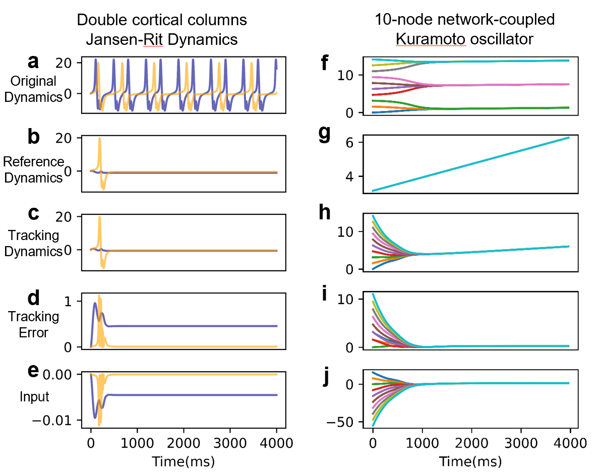
Figure 1: Two examples: (Left) Seizure suppression on the double cortical columns Jansen-Rit model. (Right) Phase synchronization on the network-coupled Kuramoto oscillator.
The controlled system exhibits a seizure-like behavior (shown in Fig. 1a). The reference dynamics are shown in Fig. 1b.
By simple calculation, we can verify that Assumption 1 & 2 hold with and . Based on Theorem 3.1, the controlled system followed the reference system if the largest eigenvalue of Eq. (15) satisfied . Thus, we take in our controller for brief. Fig. 1c shows the temporal dynamics under the proposed control strategy and Fig. 1d shows the evolution of tracking error relative to the reference dynamics. The result shows that the controlled system converged to the reference dynamics with inputs (Fig. 1e).
Further, we conduct the numerical simulations on the network-coupled Kuramoto oscillator with nodes:
(16)
The temporal dynamics of the controlled system (16) is shown in Fig 1f with parameters . The reference dynamics are generated with parameters (Fig. 1g).
With numerical analysis, Assumption 1 & 2 hold with and . Based on Theorem 3.1, the controlled system followed the reference dynamics if the largest eigenvalue of Eq. (15) satisfied . We choose in our controller. Fig. 1h shows that the dynamics of the controlled system followed the reference dynamics with small deviation controlled with calculated input (see Fig. 1i,j).
5 Conclusion
In this study, we presented a robust control strategy for manipulating the temporal dynamics of nonlinear network-coupled dynamical systems, and we demonstrated its efficacy through theoretical analysis and numerical experiments. Our approach facilitates the development of tailored control policies for personalized neurostimulation.
References
[1]
D. Sussillo, “Neural circuits as computational dynamical systems,” Current opinion in neurobiology, vol. 25, pp. 156–163, 2014.
[2]
Z. Ye, Y. Qu, Z. Liang, M. Wang, and Q. Liu, “Explainable fmri-based brain decoding via spatial temporal-pyramid graph convolutional network,” Human Brain Mapping, vol. 44, no. 7, pp. 2921–2935, 2023.
[3]
A. Ponce-Alvarez, G. Deco, P. Hagmann, G. L. Romani, D. Mantini, and M. Corbetta, “Resting-state temporal synchronization networks emerge from connectivity topology and heterogeneity,” PLoS computational biology, vol. 11, no. 2, p. e1004100, 2015.
[4]
S. Zheng, Z. Liang, Y. Qu, Q. Wu, H. Wu, and Q. Liu, “Kuramoto model-based analysis reveals oxytocin effects on brain network dynamics,” International Journal of Neural Systems, vol. 32, no. 02, p. 2250002, 2022.
[5]
M. Hemami, K. Parand, and J. A. Rad, “Numerical simulation of reaction–diffusion neural dynamics models and their synchronization/desynchronization: application to epileptic seizures,” Computers & Mathematics with Applications, vol. 78, no. 11, pp. 3644–3677, 2019.
[6]
Z. Liang, Z. Luo, K. Liu, J. Qiu, and Q. Liu, “Online learning koopman operator for closed-loop electrical neurostimulation in epilepsy,” IEEE Journal of Biomedical and Health Informatics, vol. 27, no. 1, pp. 492–503, 2023.
[7]
Y. Yang, S. Qiao, O. G. Sani, J. I. Sedillo, B. Ferrentino, B. Pesaran, and M. M. Shanechi, “Modelling and prediction of the dynamic responses of large-scale brain networks during direct electrical stimulation,” Nature biomedical engineering, vol. 5, no. 4, pp. 324–345, 2021.
[8]
K. Lou, J. Li, M. Barth, and Q. Liu, “A data-driven framework for whole-brain network modeling with simultaneous eeg-seeg data,” in International Conference on Intelligent Information Processing. Springer, 2024, pp. 329–342.
[9]
M. Wang, K. Lou, Z. Liu, P. Wei, and Q. Liu, “Multi-objective optimization via evolutionary algorithm (movea) for high-definition transcranial electrical stimulation of the human brain,” NeuroImage, vol. 280, p. 120331, 2023.
[10]
D. Cao, Q. Liu, J. Zhang, J. Li, and T. Jiang, “State-specific modulation of mood using intracranial electrical stimulation of the orbitofrontal cortex,” Brain Stimulation, vol. 16, no. 4, pp. 1112–1122, 2023.
[11]
Z. Liang, Y. Zhang, J. Wu, and Q. Liu, “Reverse engineering the brain input: Network control theory to identify cognitive task-related control nodes,” arXiv preprint arXiv:2404.16357, 2024.
[12]
G. Chen, “Pinning control of complex dynamical networks,” IEEE Transactions on Consumer Electronics, vol. 68, no. 4, pp. 336–343, 2022.
[13]
C. J. Vega, O. J. Suarez, E. N. Sanchez, G. Chen, S. Elvira-Ceja, and D. Rodriguez-Castellanos, “Trajectory tracking on complex networks via inverse optimal pinning control,” IEEE Transactions on Automatic Control, vol. 64, no. 2, pp. 767–774, 2019.
[14]
A. Zemouche and M. Boutayeb, “On lmi conditions to design observers for lipschitz nonlinear systems,” Automatica, vol. 49, no. 2, pp. 585–591, 2013.
[15]
M.-S. Chen and C.-C. Chen, “Robust nonlinear observer for lipschitz nonlinear systems subject to disturbances,” IEEE Transactions on Automatic control, vol. 52, no. 12, pp. 2365–2369, 2007.
[16]
F. Della Rossa, C. J. Vega, and P. De Lellis, “Nonlinear pinning control of stochastic network systems,” Automatica, vol. 147, p. 110712, 2023.