Leptoquark-induced CLFV decays with a light SM-singlet scalar

Abstract

The Standard Model (SM), if augmented with a light SM-singlet scalar $\phi$, 2-body charged lepton flavor violating (CLFV) decay channels can be accessed with $\phi$ as one of the final states. The effective ineteractions between $\phi$ and the SM fields can arise at TeV-scale where the governing theory extends the SM particle spectrum with a scalar leptoquark (LQ) $S_{1}$. Further, in the presence of $S_{1}$, $\phi$ can mediate 3-body CLFV processes with either two photons or two gluons in the final states. Thus, the model predicts an exotic 3-body CLFV channel: $\ell_{A}\to\ell_{B}gg$, which can be tested/constrained only through some future high-energy experiments looking for di-gluon signal from a leptonic decay.

I Introduction

At the perturbative regime, Standard Model possesses an accidental symmetry represented by the global gauge group $\mathcal{G}_{LB}\supset U(1)_{B+L}\times U(1)_{B-L}\times U(1)_{L_{\mu}-L_{\tau}}\times U(1)_{L_{\mu}+L_{\tau}-2L_{e}}$ Heeck:2016xwg which ensures the conservation of baryon number $B$ and the individual lepton numbers $L_{A}$ ($A=e,\,\mu,\,\tau$). $L=\sum_{A=e,\,\mu,\,\tau}L_{A}$ denotes the total lepton number. However, at the non-perturbative scale, the $B+L$ part of the symmetry group is broken by 6 units tHooft:1976rip . At the same time, the neutrino oscillations strongly establish that the lepton flavor can’t be a protected symmetry, resulting in a broken $U(1)_{L_{\mu}-L_{\tau}}\times U(1)_{L_{\mu}+L_{\tau}-2L_{e}}$ in the neutrino sector. The observation definitely motivates a search for similar flavor violations in the charged sector. However, for the charged leptons, $\mathcal{G}_{LB}$ is still a conserved symmetry as ensured by the Glashow-Iliopoulos-Maiani (GIM) mechanism Glashow:1970gm — any CLFV process induced by the non-zero neutrino masses and a non-trivial lepton mixing matrix will be too suppressed to detect. For example, the CLFV decay $\ell_{A}\to\ell_{B}\gamma$ induced through the Dirac neutrinos at one-loop level results in BR$(\ell_{A}\to\ell_{B}\gamma)<10^{-53}$ for all the possible channels Petcov:1976ff . Therefore, any observation of charged lepton flavor violation can be marked as a significant signature of Beyond Standard Model (BSM) contribution, as well as physics beyond neutrino oscillations.

Experimental searches for CLFV processes have been going on for a long Hincks:1948vr ; PhysRev.74.1364 , with the current sensitivity reaching $\sim\mathcal{O}(10^{-13})$ for a few flavor violating channels MEG:2016leq ; SINDRUM:1987nra ; SINDRUMII:2006dvw and being significantly improved for the others. However, in the absence of any positive signal, interest has grown in searching for CLFV decays involving low-energy BSM particles. For example, Belle-II presents the best current upper limit on $\tau\to e\phi$ and $\tau\to\mu\phi$ at 95% C.L. Belle-II:2022heu , where $\phi$ is an invisible spin-0 boson in the mass range $0-1.6$ GeV. Similar bounds for $\mu\to e\phi$ is given by Refs. TWIST:2014ymv ; Jodidio:1986mz . However, if $\phi$ decays to visible particles inside the detector, more stringent constraints could be placed from the non-observation of 3-body CLFV processes.

Various models have been proposed to address the current bounds on $\ell_{A}\to\ell_{B}\phi$, with $\phi$ being either a light scalar/pseudoscalar Wilczek:1982rv ; Grinstein:1985rt ; Berezhiani:1989fp ; Feng:1997tn ; Hirsch:2009ee ; Jaeckel:2013uva ; Celis:2014iua ; Celis:2014jua ; Galon:2016bka ; Calibbi:2016hwq ; Ema:2016ops ; Bjorkeroth:2018dzu ; Bauer:2019gfk ; Heeck:2019guh ; Cornella:2019uxs ; Calibbi:2020jvd ; Escribano:2020wua or a gauge boson Farzan:2015hkd ; Heeck:2016xkh ; Farzan:2016wym ; Ibarra:2021xyk , associated with some spontaneously broken symmetry. This paper considers $\phi$ to be a generic real SM-singlet scalar where the flavor-violating interactions arise at one-loop level in the presence of a scalar LQ $S_{1}$. LQs (for a review, see Ref. Dorsner:2016wpm ) appear naturally in the grand unified theories (GUT) Pati:1974yy ; Georgi:1974sy ; Georgi:1974my and work as an excellent BSM candidate to induce flavor violation. Though in the simplest GUT models LQs acquire mass at a scale $\Lambda_{\rm GUT}\gg\mathcal{O}(1)$ TeV, there exist GUT formulations which can ensure the stability of proton with a TeV-scale scalar LQ BUCHMULLER1986377 ; Murayama:1991ah ; Dorsner:2005fq ; GEORGI1979297 ; FileviezPerez:2007bcw ; Senjanovic:1982ex . Thus, the present paper, while extending the SM with a TeV-scale scalar LQ to describe the interactions between $\phi$ and the SM fields, effectively portrays a UV-complete theory. Ref. Mandal:2019gff has already elaborated on various CLFV observables arising in the presence of a TeV-scale scalar LQ and used the experimental upper limits to constrain the New Physics (NP) couplings. However, interesting consequences may appear if one considers a light SM-singlet scalar within the $S_{1}$-extension of SM. For example, with $M_{\phi}<(m_{\mu}-m_{e})$, $\phi$ can be produced through the on-shell decays of $\tau$ and $\mu$ leading to the CLFV processes $\tau\to\ell_{B}\phi$ [$\ell_{B}=e,\,\mu$] and $\mu\to e\phi$, respectively. In practice, the term light will be used in this paper to refer to $M_{\phi}<2m_{e}$, i.e., a sub-MeV gauge-singlet scalar. In this mass regime, it can be easily ensured that the di-lepton and di-quark decay modes of $\phi$ De:2024tbo are kinematically forbidden. However, $\phi$ can always decay to two photons at one-loop level, leading to 3-body CLFV channels of the form $\ell_{A}\to\ell_{B}\gamma\gamma$. Thus, the experimental bounds for $\ell_{A}\to\ell_{B}\gamma\gamma$ can be used to check the consistency of the parameter space allowed through the $\ell_{A}\to\ell_{B}\phi$ searches. Further, LQs being colored particles, within this proposed BSM formulation $\phi$ can also decay to two gluons. This results in a rarely discussed unconstrained CLFV decay process: $\ell_{A}\to\ell_{B}gg$. Indeed, this is a significant phenomenological outcome of this model as it predicts new CLFV observables. Therefore, any future search aiming for $\ell_{A}\to\ell_{B}gg$ will be crucial to test/falsify the model.

The rest of the paper is arranged as follows. Sec. II describes the NP interactions at the TeV scale, which connect $\phi$ with the SM fields. The analytical results for $\ell_{A}\to\ell_{B}\phi$ have been established in Sec. III. Sec. IV presents a parameter space consistent with all the existing CLFV constraints that can appear in this chosen framework and, hence, numerically analyze the detection prospects of $\ell_{A}\to\ell_{B}\phi$ within the considered mass regime. The possible decay modes of $\phi$ and the corresponding $\phi$-mediated 3-body CLFV processes have been discussed in Sec. V. Finally, the work has been concluded in Sec. VI.

II The Model: A Simple Extension of the SM

The model considers a GUT-motivated minimal extension of the SM where NP interactions arise at a scale $\Lambda_{\rm NP}\sim\mathcal{O}(1)$ TeV. The augmented particle spectrum includes a scalar LQ $S_{1}$ which transforms as ($\bar{\mathbf{3}}$, 1, 1/3) under the SM gauge group $\mathcal{G}_{\rm SM}\supset SU(3)_{C}\times SU(2)_{L}\times U(1)_{Y}$. Further, a real SM-singlet scalar $\phi$ can be proposed to exist in the sub-MeV mass regime such that its decays to the SM fields are either kinematically forbidden or highly suppressed. Defining the electromagnetic (EM) charge as $Q_{\rm EM}=T_{3}+Y$, the complete particle spectrum of the present framework has been listed in Table 1.

Fields	Generations	$SU(3)_{C}\times SU(2)_{L}\times U(1)_{Y}$
$L_{L}=(\nu_{L}\quad\ell_{L})^{T}$	3	(1, 2, -1/2)
$\ell_{R}=(e_{R},\,\mu_{R},\,\tau_{R})$	3	(1, 1, -1)
$Q_{L}=(u_{L}\quad d_{L})^{T}$	3	(3, 2, 1/6)
$U_{R}=(u_{R},\,c_{R},\,t_{R})$	3	(3, 1, 2/3)
$D_{R}=(d_{R},\,s_{R},\,b_{R})$	3	(3, 1, -1/3)
$H=(H^{+}\quad H^{0})^{T}$	1	(1, 2, 1/2)
$S_{1}$	1	($\bar{\mathbf{3}}$, 1, 1/3)
$\phi$	1	(1, 1, 0)

Table 1: Fields and their transformations under $\mathcal{G}_{\rm SM}$.

The NP interactions can be described through

$$\mathcal{L}_{\rm NP}=~{} (\mathcal{D}^{\mu}S_{1})^{\dagger}(\mathcal{D}_{\mu}S_{1})+\frac{1}{2}(\partial^{\mu}\phi)(\partial_{\mu}\phi)$$

$$-\Big{[}Y_{L}^{ij}(\bar{Q}_{L}^{Cia}\epsilon^{ab}L_{L}^{jb})S_{1}+Y_{R}^{ij}(\bar{U}_{R}^{Ci}\ell_{R}^{j})S_{1}+{\rm h.c.}\Big{]}$$

$$\qquad\qquad\qquad\qquad\qquad\qquad-\mathbb{V}(H,\,S_{1},\,\phi),$$ (1)

where $Y_{L}$ and $Y_{R}$ are completely arbitrary $3\times 3$ Yukawa matrices in the flavor basis. The superscript $C$ defines the charge-conjugated states; $\{a,b\}$ and $\{i,j\}$ stand for the $SU(2)_{L}$ and flavor indices, respectively. $\epsilon^{ab}=(i\sigma_{2})^{ab}$, $\sigma_{k}$ ($k=1,\,2,\,3$) being the Pauli matrices. The color indices have been suppressed for simplicity. Note that, the gauge interactions of $S_{1}$ can easily be obtained with an explicit definition of the covariant derivative $\mathcal{D}^{\mu}$. These interactions can be useful to produce $\phi$ at the colliders Bhaskar:2020kdr ; De:2024tbo .

The freedom to rotate equal-isospin fermion fields in the flavor basis, permits one to assume the charged lepton and down-type quark Yukawas to be diagonal so that the transformation from flavor to mass basis is given by $u_{L}\to\left(\mathbf{V}_{\rm CKM}^{\dagger}\right)u_{L}$ and $\nu_{L}\to\left(\mathbf{U}_{\rm PMNS}\right)\nu_{L}$. Here $\mathbf{V}_{\rm CKM}$ and $\mathbf{U}_{\rm PMNS}$ represent the CKM and PMNS matrices, respectively. Therefore, in the physical basis,

$$\mathcal{L}_{\rm NP} =(\mathcal{D}^{\mu}S_{1})^{\dagger}(\mathcal{D}_{\mu}S_{1})+\frac{1}{2}(\partial^{\mu}\phi)(\partial_{\mu}\phi)$$

$$-\Big{[}\left\{\bar{u}_{L}^{Ci}\left(\mathbf{V}^{*}_{\rm CKM}Y_{L}\right)^{ij}\ell_{L}^{j}\right\}S_{1}-\left\{\bar{d}_{L}^{Ci}\left(Y_{L}\mathbf{U}_{\rm PMNS}\right)^{ij}\nu_{L}^{j}\right\}S_{1}$$

$$\qquad\qquad+Y_{R}^{ij}(\bar{U}_{R}^{Ci}\ell_{R}^{j})S_{1}+{\rm h.c.}\Bigg{]}-\mathbb{V}(H,\,S_{1},\,\phi)$$

$$=(\mathcal{D}^{\mu}S_{1})^{\dagger}(\mathcal{D}_{\mu}S_{1})+\frac{1}{2}(\partial^{\mu}\phi)(\partial_{\mu}\phi)-\Big{[}\left(\bar{u}_{L}^{Ci}\xi_{L}^{ij}\ell_{L}^{j}\right)S_{1}$$

$$-\left(\bar{d}_{L}^{Ci}\chi^{ij}\nu_{L}^{j}\right)S_{1}+\xi_{R}^{ij}(\bar{U}_{R}^{Ci}\ell_{R}^{j})S_{1}+{\rm h.c.}\Bigg{]}$$

$$\qquad\qquad\qquad\qquad\qquad\qquad-\mathbb{V}(H,\,S_{1},\,\phi),$$ (2)

where, $\xi_{L}^{ij}=\left(\mathbf{V}^{*}_{\rm CKM}Y_{L}\right)^{ij}$, $\chi^{ij}=\left(Y_{L}\mathbf{U}_{\rm PMNS}\right)^{ij}$, and $\xi_{R}^{ij}=Y_{R}^{ij}$. However, the neutrino sector doesn’t play any role in the present analysis. The scalar potential can be cast as,

$$\mathbb{V} (H,\,S_{1},\,\phi)=\lambda_{HS_{1}}\left(H^{\dagger}H\right)\left(S^{\dagger}_{1}S_{1}\right)+\beta\phi\left(S^{\dagger}_{1}S_{1}\right)+\delta\phi(H^{\dagger}H)$$

$$+\lambda_{H\phi}(H^{\dagger}H)\phi^{2}+\lambda_{\phi S_{1}}\phi^{2}\left(S^{\dagger}_{1}S_{1}\right)+\frac{1}{2}M^{2}_{\phi}\phi^{2}+M^{2}_{S_{1}}\left(S^{\dagger}_{1}S_{1}\right).$$ (3)

However, one can assume $\lambda_{H\phi}$ and $\delta$ to be negligible so that the presence of $\phi$ doesn’t affect the SM scalar sector. Further, by setting $\lambda_{HS_{1}}\to 0$, one can ensure that the trilinear Higgs coupling assumes its SM-predicted value and doesn’t introduce any additional constraint to the parameter space. Note that, $\beta$ is a mass dimensional coupling which should, in principle, represent the highest scale of the theory and hence must be $\sim\mathcal{O}(1)$ TeV. After electroweak symmetry breaking (EWSB), the physical masses can be obtained via,

$$H=\frac{1}{\sqrt{2}}\begin{pmatrix}0\\ v+h\end{pmatrix},\quad\quad\phi=\phi,$$ (4)

where $h$ denotes the physical Higgs field, and $v=246$ GeV defines the electroweak vacuum expectation value (VEV). However, in the limit $\lambda_{HS_{1}}\to 0$ and $\lambda_{H\phi}\to 0$, $M_{S_{1}}$ and $M_{\phi}$ represent the physical masses of $S_{1}$ and $\phi$, respectively.

III Lepton Flavor Violation: $\boldsymbol{\Large\ell_{A}\to\ell_{B}+\phi}$

The proposed model, which extends the SM with a scalar LQ $S_{1}$, possesses a rich BSM phenomenology in the lepton sector. For example, the discrepancies in muon and electron $(g-2)$, semi-leptonic decays, non-observation of CLFV processes including $\ell_{A}\to\ell_{B}\gamma$, $\ell_{A}\to\bar{\ell}_{B}\ell_{B}\ell_{B}$, $h\to\bar{\ell}_{A}\ell_{B}$, and $\mu-e$ conversion can be explained with $M_{S_{1}}\sim\mathcal{O}(1)$ TeV. However, in the presence of an additional light SM-singlet scalar, new CLFV channels can be introduced within the considered framework where the SM leptons ($\tau$ and $\mu$) can decay to $\phi$ and a lighter lepton through the effective vertex shown in Fig. 1. To be specific, for $M_{\phi}\leq 1$ MeV, $\tau\to e\phi$, $\tau\to\mu\phi$, and $\mu\to e\phi$ CLFV modes are kinematically accessible.

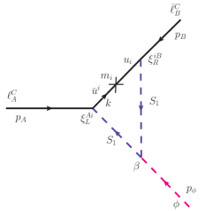
Figure 1: Leading order contribution to $\ell_{A}\to\ell_{B}\phi$. Here, $k$ denotes the loop momentum, and $p_{A}=-(p_{B}+p_{\phi})$ defines the momentum conservation.

The effective coupling corresponding to Fig. 1 is given by,

$$-i Y_{\ell_{A}\ell_{B}\phi}=\sum_{i=\,u,c,t}(\xi_{L}^{Ai})^{*}\xi_{R}^{iB}\beta m_{i}\int\frac{d^{4}k}{(2\pi)^{4}}\Bigg{[}\frac{(k^{2}+m_{i}^{2})}{(k^{2}-m_{i}^{2})^{2}}\times$$

$$\qquad\qquad\frac{1}{\{(k+p_{B})^{2}-M_{S_{1}}^{2}\}\{(k+p_{B}+p_{\phi})^{2}-M_{S_{1}}^{2}\}}\Bigg{]}$$

$$= \sum_{i=\,u,c,t}(\xi_{L}^{Ai})^{*}\xi_{R}^{iB}\beta m_{i}\int\frac{d^{4}k}{(2\pi)^{4}}\Bigg{[}$$

$$\frac{1}{(k^{2}-m_{i}^{2})\{(k+p_{B})^{2}-M_{S_{1}}^{2}\}\{(k+p_{B}+p_{\phi})^{2}-M_{S_{1}}^{2}\}}$$

$$+\frac{2m_{i}^{2}}{(k^{2}-m_{i}^{2})^{2}\{(k+p_{B})^{2}-M_{S_{1}}^{2}\}\{(k+p_{B}+p_{\phi})^{2}-M_{S_{1}}^{2}\}}\Bigg{]}$$

$$= \left(\frac{i\,\beta}{16\pi^{2}}\right)\sum_{i=\,u,c,t}\Omega^{AB}_{i}\,m_{i}\,\Bigg{[}\mathcal{J}_{1}+2m_{i}^{2}\times\mathcal{J}_{2}\Bigg{]},$$ (5)

where $\Omega^{AB}_{i}=(\xi_{L}^{Ai})^{*}\xi_{R}^{iB}$, and

$$\mathcal{J}_{1}= \ -C_{0}\left(m_{B}^{2},\,M_{\phi}^{2},\,m_{A}^{2},\,m_{i}^{2},\,M_{S_{1}}^{2},\,M_{S_{1}}^{2}\right),$$

$$\mathcal{J}_{2}= \ D_{0}\left(0,\,m_{B}^{2},\,M_{\phi}^{2},\,m_{A}^{2},\,m_{B}^{2},\,m_{A}^{2},\,m_{i}^{2},\,m_{i}^{2},\,M_{S_{1}}^{2},\,M_{S_{1}}^{2}\right).$$ (6)

Eq. (5) has been obtained assuming an on-shell decay of $\ell_{A}$ so that $p_{A}^{2}=(p_{B}+p_{\phi})^{2}=m_{A}^{2}$. Here, $C_{0}$ and $D_{0}$ denote the standard Passarino-Veltmen functions Romao:2020 ; Hahn:1998yk for the scalar 3-point and 4-point one-loop integrals, respectively.

In the rest-frame of $\ell_{A}$, the decay width for $\ell_{A}\to\ell_{B}\phi$ can be calculated as,

$$\Gamma(\ell_{A}\to\ell_{B}\phi)= ~{}\frac{\mathcal{N}_{C}\times|Y_{\ell_{A}\ell_{B}\phi}|^{2}}{16\pi}\times m_{A}\times\Big{[}(1+\rho_{B})^{2}-\rho_{\phi}^{2}\Big{]}$$

$$\times\Bigg{[}\Big{\{}1-(\rho_{\phi}+\rho_{B})^{2}\Big{\}}\Big{\{}1-(\rho_{\phi}-\rho_{B})^{2}\Big{\}}\Bigg{]}^{1/2}\,,$$ (7)

where $\rho_{B}=m_{B}/m_{A}$, and $\rho_{\phi}=M_{\phi}/m_{A}$. $\mathcal{N}_{C}=3$ stands for the color degeneracy factor. However, to detect any signal from $\ell_{A}\to\ell_{B}\phi$ decay, $\ell_{A}\to\ell_{B}\bar{\nu}_{B}\nu_{A}$ acts as the strongest background. Therefore, to parametrize the detectability of $\ell_{A}\to\ell_{B}\phi$ over $\ell_{A}\to\ell_{B}\bar{\nu}_{B}\nu_{A}$, a variable $R_{AB}$ can be defined as,

$$R_{AB}=\frac{{\rm BR}(\ell_{A}\to\ell_{B}\phi)}{{\rm BR}(\ell_{A}\to\ell_{B}\bar{\nu}_{B}\nu_{A})},$$ (8)

where BR symbolizes the branching ratio for a particular decay mode. In the subsequent analysis, $R_{AB}$ will be considered as a good observable to constrain the parameter space.

IV Numerical Analysis

As stated in Sec. III, the $S_{1}$-extension of SM can accommodate several BSM observations and possibilities resulting in strong bounds on the NP couplings $\xi^{ij}_{L,R}$. Thus, to analyze the $\ell_{A}\to\ell_{B}\phi$ processes, one must choose a parameter space consistent with all the existing leptonic constraints. Following Ref. Mandal:2019gff , Table 2 enlists the most stringent upper limits on $|\Omega^{AB}_{i}|^{2}$ relavent for the present study.

CLFV	$|\Omega^{AB}_{i}|^{2}$	Experimental	Considered
Processes		Bounds $\times\left(M_{S_{1}}/{\rm TeV}\right)^{4}$	Values
	$|\Omega^{\tau e}_{u}|^{2}$	$<\,3.0\times 10^{-6}$ ParticleDataGroup:2018ovx	$10^{-6}$
$\tau\to e\phi$	$|\Omega^{\tau e}_{c}|^{2}$	$<\,2.1\times 10^{-4}$ BaBar:2009hkt	$10^{-6}$
	$|\Omega^{\tau e}_{t}|^{2}$	$<\,3.8\times 10^{-7}$ BaBar:2009hkt	$[10^{-12},\,10^{-6}]$
	$|\Omega^{\tau\mu}_{u}|^{2}$	$<\,5.7\times 10^{-6}$ ParticleDataGroup:2018ovx	$10^{-6}$
$\tau\to\mu\phi$	$|\Omega^{\tau\mu}_{c}|^{2}$	$<\,2.8\times 10^{-4}$ BaBar:2009hkt	$10^{-6}$
	$|\Omega^{\tau\mu}_{t}|^{2}$	$<\,5.0\times 10^{-7}$ BaBar:2009hkt	$[10^{-12},\,10^{-6}]$
	$|\Omega^{\mu e}_{u}|^{2}$	$<\,6.7\times 10^{-12}$ SINDRUMII:2006dvw	$10^{-12}$
$\mu\to e\phi$	$|\Omega^{\mu e}_{c}|^{2}$	$<\,1.7\times 10^{-12}$ MEG:2016leq	$[10^{-16},\,10^{-12}]$
	$|\Omega^{\mu e}_{t}|^{2}$	$<\,3.0\times 10^{-15}$ MEG:2016leq	$10^{-17}$

Table 2: Experimental constraints on the NP couplings and their considered values used for the computations.

The first column of Table 2 specifies a particular $\ell_{A}\to\ell_{B}\phi$ process, while the third column represents the experimental bounds on the associated NP couplings arising through the other CLFV processes. However, the bounds drastically deteriorate with increasing LQ mass. Thus, in general, the couplings considered for the present analysis assume $M_{S_{1}}\geq 2$ TeV and have been listed in the last column of Table 2. As an illustrative choice, $\beta=5$ TeV will be used for the analysis.

IV.1 $\boldsymbol{\tau}$-Sector

The $\tau e\phi$ and $\tau\mu\phi$ effective couplings can be obtained from Eq. (5) with $m_{A}=m_{\tau}$ and $m_{B}=m_{e},\,m_{\mu}$, respectively. Fig. 2 shows their variations with increasing LQ mass. All the NP couplings $\Omega^{\tau B}_{i}$ have been fixed at their respective upper limits, i.e., $10^{-3}$, while $M_{\phi}$ has been randomly varied between 1 keV and 1 MeV to generate Fig. 2.

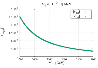
Figure 2: Variation of $|Y_{\tau e\phi}|$ (red) and $|Y_{\tau\mu\phi}|$ (green) as a function of $M_{S_{1}}$ with $M_{\phi}\in[1~{}{\rm keV},1~{}{\rm MeV}]$.

However, the results suggest that the variation of $M_{\phi}$ in the considered range negligibly affects $|Y_{\tau\ell_{B}\phi}|$ ($\ell_{B}=e,\,\mu$). Further, the lighter lepton masses (i.e., $m_{e}$ and $m_{\mu}$) being ignorable with respect to $\Lambda_{\rm NP}$, $|Y_{\tau e\phi}|$ and $|Y_{\tau\mu\phi}|$ overlap.

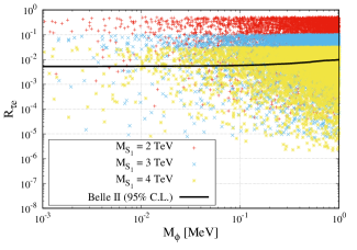
((a))     (a)

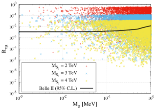
((b))     (b)

Figure 3: Variation of (a) $R_{\tau e}$, and (b) $R_{\tau\mu}$ as a function of $M_{\phi}$ for $M_{S_{1}}=2$ TeV (red), 3 TeV (sky), and 4 TeV (yellow). The solid black lines denote the observed upper limits (at 95% C.L.) from Belle II collaboration Belle-II:2022heu .

Fig. 3 (a) and 3 (b) display the variation of $R_{\tau e}$ and $R_{\tau\mu}$ as a function of $M_{\phi}$, resepectively. For Fig. 3 (a), $\Omega^{\tau e}_{t}$ has been randomly varied within the range $[10^{-6},\,10^{-3}]$, whereas one has to vary $\Omega^{\tau\mu}_{t}$ to generate the scattered plot in Fig. 3 (b). Currently, the most stringent bounds on $R_{\tau\ell_{B}}$ are set by Belle II collaboration Belle-II:2022heu as shown by the solid black lines in Fig. 3. The results indicate a significant parameter space where the non-observation of $\tau\to e\phi$ and $\tau\to\mu\phi$ can be explained along with the other CLFV processes. Moreover, the allowed parameter space improves with a heavier $S_{1}$.

IV.2 $\boldsymbol{\mu}$-Sector

$\phi$ being in the sub-MeV mass regime, $\mu$ can also decay to $\phi$ and $e$ through the effective $Y_{\mu e\phi}$ coupling. Fig. 4 depicts its variation as a function of $M_{S_{1}}$. As before, all the NP couplings have been fixed at their allowed upper bounds with $M_{\phi}$ varying randomly within the range 1 keV to 1 MeV.

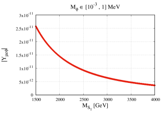
Figure 4: Variation of $|Y_{\mu e\phi}|$ as a function of $M_{S_{1}}$ with $M_{\phi}\in[1~{}{\rm keV},1~{}{\rm MeV}]$.

Note that, $|Y_{\mu e\phi}/Y_{\tau\ell_{B}\phi}|\sim 10^{-5}$. The large suppression for $Y_{\mu e\phi}$ stems from the NP couplings $\Omega^{\mu e}_{i}$ ($i=u,\,c,\,t$), which are tightly constrained through the experimental bounds on $\mu\to e\gamma$ MEG:2016leq and $\mu-e$ conversion on gold nuclei SINDRUMII:2006dvw .

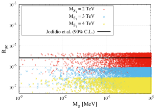
Figure 5: Variation of $R_{\mu e}$ as a function of $M_{\phi}$ for $M_{S_{1}}=2$ TeV (red), 3 TeV (sky), and 4 TeV (yellow). The black solid line marks the observed upper limit (at 90% C.L.) from Jodidio et al. Jodidio:1986mz .

Fig. 5 presents the $M_{\phi}$ dependence of $R_{\mu e}$ for three different LQ masses. The plot has been generated through a random variation of $\Omega^{\mu e}_{c}$ within the range $[10^{-8},\,10^{-6}]$, whereas $\Omega^{\mu e}_{u}$ and $\Omega^{\mu e}_{t}$ have been fixed at $10^{-6}$ and $3.16\times 10^{-9}$, respectively.

TWIST collaboration sets the most stringent bound on $R_{\mu e}$, when $\phi$ is a massive invisible boson in the range $13-80$ MeV TWIST:2014ymv . However, in the sub-MeV mass regime, $\phi$ can be treated as effectively massless, and hence, the best experimental upper limit can be read as $R_{\mu e}<2.6\times 10^{-6}$ (Jodidio et al. Jodidio:1986mz ). Thus, in Fig. 5, the portion below the black solid line defines the allowed parameter space for $\mu\to e\phi$.

V Decay of $\boldsymbol{\phi}$ and Other CLFV Constraints

As indicated in the Introduction, Refs. Jodidio:1986mz ; TWIST:2014ymv ; Belle-II:2022heu set the best constraints for the considered 2-body CLFV decays if $\phi$ is an invisible light boson, i.e., either $\phi$ decays to invisible particles (e.g., dark matter, neutrinos) or features a significantly large decay-length. In the former case, only a sharp energy peak of electron or muon can be searched over the continuous Michel spectrum. However, if $\phi$ decays to visible particles, there is always a chance to have better constraints from the 3-body CLFV processes.

In the proposed framework, the gauge-singlet scalar $\phi$ produced through the on-shell decays of $\tau$ and/or $\mu$ can further decay via di-photon and di-gluon channels with the leading order contributions arising at one-loop level [see Fig. 6]. Note that, for $M_{\phi}<2m_{e}$, other decay modes of $\phi$ are kinematically forbidden.

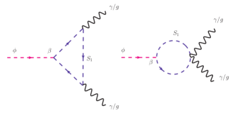
Figure 6: Leading order contributions to $\phi\to\gamma\gamma\,(gg)$ processes.

Thus, the total decay width of $\phi$ can be formulated as,

$$\Gamma_{\phi}=\Gamma(\phi\to gg)+\Gamma(\phi\to\gamma\gamma),$$ (9)

where the partial decay widths are given by Dorsner:2016wpm ; Bhaskar:2020kdr ,

$$\Gamma(\phi\rightarrow gg) \ =\ \frac{G_{\rm F}\alpha_{S}^{2}M_{\phi}^{3}}{64\sqrt{2}\pi^{3}}\left|\frac{\beta v}{2M_{S_{1}}^{2}}\mathcal{P}\left(\frac{M_{\phi}^{2}}{4M_{S_{1}}^{2}}\right)\right|^{2},$$

$$\Gamma(\phi\rightarrow\gamma\gamma) \ =\ \frac{G_{\rm F}\alpha_{\rm EM}^{2}M_{\phi}^{3}}{128\sqrt{2}\pi^{3}}\left|\frac{\beta v}{6M_{S_{1}}^{2}}\mathcal{P}\left(\frac{M_{\phi}^{2}}{4M_{S_{1}}^{2}}\right)\right|^{2}.$$ (10)

Here, $G_{\rm F}$ is the Fermi constant, $\alpha_{S}$ and $\alpha_{\rm EM}$ define the strong and electromagnetic coupling constants, respectively. The function $\mathcal{P}$ can be defined as,

$$\mathcal{P}(x)=-\frac{[x-\psi(x)]}{x^{2}}\,,$$ (11)

where,

$$\psi(x) =\Bigg{\{}\begin{array}[]{cc}{\rm Arcsin}^{2}(\sqrt{x}),&x\leq 1\\ -\frac{1}{4}\left[{\rm ln}\left(\frac{1+\sqrt{1-x^{-1}}}{1-\sqrt{1-x^{-1}}}\right)-i\pi\right]^{2},&x>1\,.\end{array}$$ (14)

Thus, the proposed framework opens up 3-body CLFV decay routes of the form $\ell_{A}\to\ell_{B}\gamma\gamma$ and $\ell_{A}\to\ell_{B}gg$, which can possibly be used to check the validity of the available parameter space. However, the former decay channel, where the heavier lepton decays to a lighter one and two photons, is well-known in the literature and has also been explored through experiments, whereas the latter is mostly unconstrained and rarely discussed in theory.

$\Gamma_{\phi}$ being extremely suppressed $\left(\leq\mathcal{O}(10^{-22})~{}{\rm GeV}\right)$, one can use the narrow width approximation to study the $\phi$-mediated 3-body CLFV decays Cordero-Cid:2005vca . Therefore, the corresponding branching ratios can be cast as,

$${\rm BR}(\ell_{A}\to\ell_{B}XX)\simeq{\rm BR}(\ell_{A}\to\ell_{B}\phi)\times{\rm BR}(\phi\to XX),$$ (15)

where $X$ represents either photon or gluon.

V.1 $\boldsymbol{\ell_{A}\to\ell_{B}\gamma\gamma}$

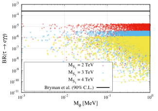
((a))     (a)

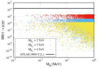
((b))     (b)

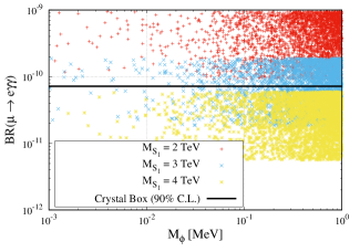
((c))     (c)

Figure 7: Variation of (a) BR$(\tau\to e\gamma\gamma)$, (b) BR$(\tau\to\mu\gamma\gamma)$, and (c) BR$(\mu\to e\gamma\gamma)$ as a function of $M_{\phi}$ for $M_{S_{1}}=2$ TeV (red), 3 TeV (sky), and 4 TeV (yellow). The black solid lines represent the corresponding experimental sentitivities (at 90% C.L.).

This type of 3-body CLFV processes have been searched for a long time (particularly for $\mu\to e\gamma\gamma$) through various experiments, and till now, no flavor violation has been observed. Thus, the null results have set certain upper limits on BR($\ell_{A}\to\ell_{B}\gamma\gamma$), which may further propagate into the $(\ell_{A}\to\ell_{B}\phi)$-allowed parameter space as more stringent constraints. Table 3 presents the current experimental bounds on BR($\ell_{A}\to\ell_{B}\gamma\gamma$).

CLFV Observables	Upper Limits	Experiments
BR($\mu\to e\gamma\gamma$)	$7.2\times 10^{-11}$	Crystal Box Bolton:1988af
BR($\tau\to e\gamma\gamma$)	$2.5\times 10^{-4}$	Bryman et al. Bryman:2021ilc
BR($\tau\to\mu\gamma\gamma$)	$1.5\times 10^{-4}$	ATLAS Angelozzi:2017oeg

Table 3: Experimental bounds on $\ell_{A}\to\ell_{B}\gamma\gamma$ processes.

Clearly, the experimental bounds for BR$(\tau\to\ell_{B}\gamma\gamma)$ [$\ell_{B}=e,\,\mu$] are less stringent compared to those on $R_{\tau\ell_{B}}$ from Belle-II. It can be easily understood from Fig. 7 (a) and 7 (b) that the 3-body decay doesn’t add any additional constraint in the $\tau$-sector, and effectively the entire parameter space is allowed with the existing upper limits. Therefore, Fig. 3 alone displays the actual permitted region where the production prospects of $\phi$ via $\tau$-decays can be studied. Fig. 7 (c) depicts the $M_{\phi}$ dependence of BR$(\mu\to e\gamma\gamma)$ for different values of $M_{S_{1}}$. The currently available experimental sensitivity restricts BR$(\mu\to e\gamma\gamma)<7.2\times 10^{-11}$ Bolton:1988af and, thus, introduces the strongest bound on the considered parameter space. With all the $(\mu\to e\phi)$-specific NP couplings (i.e., $|\Omega^{\mu e}_{i}|$) being fixed at their allowed values/ranges as listed in Table 2, the results show that a sub-MeV SM-singlet scalar can only be produced through the flavor violating muon decay if $M_{S_{1}}>2$ TeV.

V.2 $\boldsymbol{\ell_{A}\to\ell_{B}gg}$

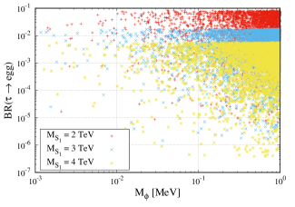
((a))     (a)

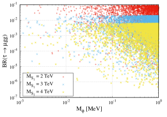
((b))     (b)

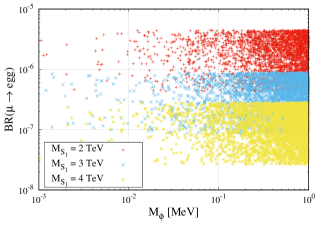
((c))     (b)

Figure 8: Variation of (a) BR$(\tau\to e\,gg)$, (b) BR$(\tau\to\mu\,gg)$, and (c) BR$(\mu\to e\,gg)$ as a function of $M_{\phi}$ for $M_{S_{1}}=2$ TeV (red), 3 TeV (sky), and 4 TeV (yellow).

The proposed extension of SM can accommodate an exotic 3-body CLFV channel where the heavier charged leptons can decay to the lighter ones and two gluons. To the best of the author’s knowledge, very little has been explored about this particular type of CLFV decays, as they can never be probed through low-energy experiments. Colliders using deep inelastic scattering can only be an option to search for $\ell_{A}\to\ell_{B}gg$ AbdulKhalek:2022hcn . For example, Refs. Takeuchi:2017btl ; Cirigliano:2021img have discussed the gluonic contribution to the $\tau$-specific CLFV processes in an Electron Ion/Proton Collider.

Therefore, these decays might lead to completely new observables for probing the lepton flavor violation in the charged sector. Fig. 8 shows the model predictions for $\tau\to egg$, $\tau\to\mu gg$, and $\mu\to egg$. Note that, ${\rm BR}(\ell_{A}\to\ell_{B}gg)/{\rm BR}(\ell_{A}\to\ell_{B}\gamma\gamma)\sim\mathcal{O}(10^{3})$ as $\phi$ dominantly decays through the di-gluon channel. Therefore, in principle, $\ell_{A}\to\ell_{B}gg$ should have a better detection prospect compared to $\ell_{A}\to\ell_{B}\gamma\gamma$ if the background is substantially reduced ATL-PHYS-PUB-2017-017 ; CMS-DP-2017-027 ; Andrews:2019faz . Though, currently, there is no direct experimental bound for these processes, detectors looking for di-gluon signals from CLFV decays may test/falsify the present predictions in the future.

VI Conclusion

By the next decade, experiments searching for CLFV processes is going to play a vital role in discovering physics beyond the SM. The chances will definitely enhance with the increasing number CLFV observables. Moreover, the observation will also be significant in understanding the possible NP theory associated with such a positive signal. This paper has extended the SM with a light SM-singlet scalar $\phi$ with mass $M_{\phi}<2m_{e}$. There is a wide range of theories where such a generic scalar can be associated with a spontaneously broken global symmetry. The effective couplings of $\phi$ with the SM fields can be obtained at one-loop level in the presence of a TeV-scale scalar LQ $S_{1}$. Phenomenologically, scalar LQs are well-motivated hypothetical particles that generate a large variety of CLFV processes. Thus, the non-observation of any CLFV process with the existing experimental sensitivities results in stringent constraints on the NP couplings at the quark-LQ-lepton vertices. Considering such a pre-constrained parameter space, the present paper has studied the discovery prospects of $\tau\to e\phi$, $\tau\to\mu\phi$, and $\mu\to e\phi$. Though for illustrations, 1 keV $\leq M_{\phi}\leq$ 1 MeV has been chosen, the results are equally valid for any generic scalar lighter than $2m_{e}$. $S_{1}$ being an EM-charged color-triplet scalar, $\phi$ can decay through di-photon and di-gluon channels. This induces the possibility of 3-body CLFV decays $\ell_{A}\to\ell_{B}\gamma\gamma$ and $\ell_{A}\to\ell_{B}gg$, where $\phi$ acts as the mediator. Though for the $\tau$-sector, the experimental bounds on $\tau\to\ell_{B}\gamma\gamma$ [$\ell_{B}=e,\,\mu$] are less stringent compared to those on the $\tau\to\ell_{B}\phi$, for $\mu$-sector BR$(\mu\to e\gamma\gamma)$ becomes crucial to constrain the parameter space. The most remarkable feature of this model is the possibility to predict CLFV observables corresponding to the 3-body decay $\ell_{A}\to\ell_{B}gg$, for all the possible channels. No direct experimental limit exists for such leptonic decays with two gluons in the final states. Using narrow-width approximation, the model has predicted for BR$(\tau\to egg)$, BR$(\tau\to\mu gg)$, and BR$(\mu\to egg)$ within the allowed parameter space. Therefore, a future experiment searching for $\ell_{A}\to\ell_{B}gg$ will be significant to test/constrain the model or may lead to a discovery.

References

- (1) J. Heeck, Interpretation of Lepton Flavor Violation, Phys. Rev. D 95 (2017) 015022, [1610.07623].
- (2) G. ’t Hooft, Symmetry Breaking Through Bell-Jackiw Anomalies, Phys. Rev. Lett. 37 (1976) 8–11.
- (3) S. L. Glashow, J. Iliopoulos and L. Maiani, Weak Interactions with Lepton-Hadron Symmetry, Phys. Rev. D 2 (1970) 1285–1292.
- (4) S. T. Petcov, The Processes in the Weinberg-Salam Model with Neutrino Mixing, Sov. J. Nucl. Phys. 25 (1977) 340. [Erratum: Sov.J.Nucl.Phys. 25, 698 (1977), Erratum: Yad.Fiz. 25, 1336 (1977)].
- (5) E. P. Hincks and B. Pontecorvo, Search for gamma-radiation in the 2.2-microsecond meson decay process, Phys. Rev. 73 (1948) 257–258.
- (6) R. D. Sard and E. J. Althaus, A search for delayed photons from stopped sea level cosmic-ray mesons, Phys. Rev. 74 (Nov, 1948) 1364–1371.
- (7) MEG collaboration, A. M. Baldini et al., Search for the lepton flavour violating decay with the full dataset of the MEG experiment, Eur. Phys. J. C 76 (2016) 434, [1605.05081].
- (8) SINDRUM collaboration, U. Bellgardt et al., Search for the Decay , Nucl. Phys. B 299 (1988) 1–6.
- (9) SINDRUM II collaboration, W. H. Bertl et al., A Search for muon to electron conversion in muonic gold, Eur. Phys. J. C 47 (2006) 337–346.
- (10) Belle-II collaboration, I. Adachi et al., Search for Lepton-Flavor-Violating Decays to a Lepton and an Invisible Boson at Belle II, Phys. Rev. Lett. 130 (2023) 181803, [2212.03634].
- (11) TWIST collaboration, R. Bayes et al., Search for two body muon decay signals, Phys. Rev. D 91 (2015) 052020, [1409.0638].
- (12) A. Jodidio et al., Search for Right-Handed Currents in Muon Decay, Phys. Rev. D 34 (1986) 1967. [Erratum: Phys.Rev.D 37, 237 (1988)].
- (13) F. Wilczek, Axions and Family Symmetry Breaking, Phys. Rev. Lett. 49 (1982) 1549–1552.
- (14) B. Grinstein, J. Preskill and M. B. Wise, Neutrino Masses and Family Symmetry, Phys. Lett. B 159 (1985) 57–61.
- (15) Z. G. Berezhiani and M. Y. Khlopov, Cosmology of Spontaneously Broken Gauge Family Symmetry, Z. Phys. C 49 (1991) 73–78.
- (16) J. L. Feng, T. Moroi, H. Murayama and E. Schnapka, Third generation familons, b factories, and neutrino cosmology, Phys. Rev. D 57 (1998) 5875–5892, [hep-ph/9709411].
- (17) M. Hirsch, A. Vicente, J. Meyer and W. Porod, Majoron emission in muon and tau decays revisited, Phys. Rev. D 79 (2009) 055023, [0902.0525]. [Erratum: Phys.Rev.D 79, 079901 (2009)].
- (18) J. Jaeckel, A Family of WISPy Dark Matter Candidates, Phys. Lett. B 732 (2014) 1–7, [1311.0880].
- (19) A. Celis, J. Fuentes-Martin and H. Serodio, An invisible axion model with controlled FCNCs at tree level, Phys. Lett. B 741 (2015) 117–123, [1410.6217].
- (20) A. Celis, J. Fuentes-Martín and H. Serôdio, A class of invisible axion models with FCNCs at tree level, JHEP 12 (2014) 167, [1410.6218].
- (21) I. Galon, A. Kwa and P. Tanedo, Lepton-Flavor Violating Mediators, JHEP 03 (2017) 064, [1610.08060].
- (22) L. Calibbi, F. Goertz, D. Redigolo, R. Ziegler and J. Zupan, Minimal axion model from flavor, Phys. Rev. D 95 (2017) 095009, [1612.08040].
- (23) Y. Ema, K. Hamaguchi, T. Moroi and K. Nakayama, Flaxion: a minimal extension to solve puzzles in the standard model, JHEP 01 (2017) 096, [1612.05492].
- (24) F. Björkeroth, E. J. Chun and S. F. King, Flavourful Axion Phenomenology, JHEP 08 (2018) 117, [1806.00660].
- (25) M. Bauer, M. Neubert, S. Renner, M. Schnubel and A. Thamm, Axionlike Particles, Lepton-Flavor Violation, and a New Explanation of and , Phys. Rev. Lett. 124 (2020) 211803, [1908.00008].
- (26) J. Heeck and H. H. Patel, Majoron at two loops, Phys. Rev. D 100 (2019) 095015, [1909.02029].
- (27) C. Cornella, P. Paradisi and O. Sumensari, Hunting for ALPs with Lepton Flavor Violation, JHEP 01 (2020) 158, [1911.06279].
- (28) L. Calibbi, D. Redigolo, R. Ziegler and J. Zupan, Looking forward to lepton-flavor-violating ALPs, JHEP 09 (2021) 173, [2006.04795].
- (29) P. Escribano and A. Vicente, Ultralight scalars in leptonic observables, JHEP 03 (2021) 240, [2008.01099].
- (30) Y. Farzan and I. M. Shoemaker, Lepton Flavor Violating Non-Standard Interactions via Light Mediators, JHEP 07 (2016) 033, [1512.09147].
- (31) J. Heeck, Lepton flavor violation with light vector bosons, Phys. Lett. B 758 (2016) 101–105, [1602.03810].
- (32) Y. Farzan and J. Heeck, Neutrinophilic nonstandard interactions, Phys. Rev. D 94 (2016) 053010, [1607.07616].
- (33) A. Ibarra, M. Marín and P. Roig, Flavor violating muon decay into an electron and a light gauge boson, Phys. Lett. B 827 (2022) 136933, [2110.03737].
- (34) I. Doršner, S. Fajfer, A. Greljo, J. F. Kamenik and N. Košnik, Physics of leptoquarks in precision experiments and at particle colliders, Phys. Rept. 641 (2016) 1–68, [1603.04993].
- (35) J. C. Pati and A. Salam, Lepton Number as the Fourth Color, Phys. Rev. D 10 (1974) 275–289. [Erratum: Phys.Rev.D 11, 703–703 (1975)].
- (36) H. Georgi and S. L. Glashow, Unity of All Elementary Particle Forces, Phys. Rev. Lett. 32 (1974) 438–441.
- (37) H. Georgi, The State of the Art—Gauge Theories, AIP Conf. Proc. 23 (1975) 575–582.
- (38) W. Buchmuller and D. Wyler, Constraints on su(5)-type leptoquarks, Physics Letters B 177 (1986) 377 – 382.
- (39) H. Murayama and T. Yanagida, A viable SU(5) GUT with light leptoquark bosons, Mod. Phys. Lett. A 7 (1992) 147–152.
- (40) I. Dorsner and P. Fileviez Perez, Unification without supersymmetry: Neutrino mass, proton decay and light leptoquarks, Nucl. Phys. B 723 (2005) 53–76, [hep-ph/0504276].
- (41) H. Georgi and C. Jarlskog, A new lepton-quark mass relation in a unified theory, Physics Letters B 86 (1979) 297–300.
- (42) P. Fileviez Perez, Renormalizable adjoint SU(5), Phys. Lett. B 654 (2007) 189–193, [hep-ph/0702287].
- (43) G. Senjanovic and A. Sokorac, Light Leptoquarks in SO(10), Z. Phys. C 20 (1983) 255.
- (44) R. Mandal and A. Pich, Constraints on scalar leptoquarks from lepton and kaon physics, JHEP 12 (2019) 089, [1908.11155].
- (45) B. De, Direct production of SM-singlet scalars at the muon collider, Phys. Lett. B 852 (2024) 138634, [2401.08101].
- (46) A. Bhaskar, D. Das, B. De and S. Mitra, Enhancing scalar productions with leptoquarks at the LHC, Phys. Rev. D 102 (2020) 035002, [2002.12571].
- (47) J. C. Romo, “Advanced Quantum Field Theory.” https://porthos.tecnico.ulisboa.pt/Public/textos/tca.pdf, 2020.
- (48) T. Hahn and M. Perez-Victoria, Automatized one loop calculations in four-dimensions and D-dimensions, Comput. Phys. Commun. 118 (1999) 153–165, [hep-ph/9807565].
- (49) Particle Data Group collaboration, M. Tanabashi et al., Review of Particle Physics, Phys. Rev. D 98 (2018) 030001.
- (50) BaBar collaboration, B. Aubert et al., Searches for Lepton Flavor Violation in the Decays and , Phys. Rev. Lett. 104 (2010) 021802, [0908.2381].
- (51) A. Cordero-Cid, G. Tavares-Velasco and J. J. Toscano, Implications of a very light pseudoscalar boson on lepton flavor violation, Phys. Rev. D 72 (2005) 117701, [hep-ph/0511331].
- (52) R. D. Bolton et al., Search for Rare Muon Decays with the Crystal Box Detector, Phys. Rev. D 38 (1988) 2077.
- (53) D. A. Bryman, S. Ito and R. Shrock, Upper limits on branching ratios of the lepton-flavor-violating decays and , Phys. Rev. D 104 (2021) 075032, [2106.02451].
- (54) I. Angelozzi, In pursuit of lepton flavour violation : A search for the decay with ATLAS at =8 TeV. PhD thesis, U. Amsterdam, IHEF, 2017.
- (55) R. Abdul Khalek et al., Snowmass 2021 White Paper: Electron Ion Collider for High Energy Physics, 2203.13199.
- (56) M. Takeuchi, Y. Uesaka and M. Yamanaka, Higgs mediated CLFV processes N ( eN )→ X via gluon operators, Phys. Lett. B 772 (2017) 279–282, [1705.01059].
- (57) V. Cirigliano, K. Fuyuto, C. Lee, E. Mereghetti and B. Yan, Charged Lepton Flavor Violation at the EIC, JHEP 03 (2021) 256, [2102.06176].
- (58) ATLAS collaboration, “Quark versus Gluon Jet Tagging Using Jet Images with the ATLAS Detector.” https://cds.cern.ch/record/2275641, 2017.
- (59) CMS collaboration, “New Developments for Jet Substructure Reconstruction in CMS.” https://cds.cern.ch/record/2275226, 2017.
- (60) M. Andrews, J. Alison, S. An, P. Bryant, B. Burkle, S. Gleyzer et al., End-to-end jet classification of quarks and gluons with the CMS Open Data, Nucl. Instrum. Meth. A 977 (2020) 164304, [1902.08276].