Nonlinear classification of neural manifolds with contextual information

Abstract

Understanding how neural systems efficiently process information through distributed representations is a fundamental challenge at the interface of neuroscience and machine learning. Recent approaches analyze the statistical and geometrical attributes of neural representations as population-level mechanistic descriptors of task implementation. In particular, manifold capacity has emerged as a promising framework linking population geometry to the separability of neural manifolds. However, this metric has been limited to linear readouts. Here, we propose a theoretical framework that overcomes this limitation by leveraging contextual input information. We derive an exact formula for the context-dependent capacity that depends on manifold geometry and context correlations, and validate it on synthetic and real data. Our framework’s increased expressivity captures representation untanglement in deep networks at early stages of the layer hierarchy, previously inaccessible to analysis. As context-dependent nonlinearity is ubiquitous in neural systems, our data-driven and theoretically grounded approach promises to elucidate context-dependent computation across scales, datasets, and models.

Introduction. Understanding the neural population code that underlies efficient representations is crucial for neuroscience and machine learning. Approaches focused on the geometry of task structures in neural population activities have recently emerged as a promising direction for understanding information processing in neural systems Chung and Abbott (2021); Sorscher et al. (2022); Bernardi et al. (2020); Ansuini et al. (2019). Notably, analytical advances linking representation geometry to the capacity of the downstream readout Chung et al. (2018); Wakhloo et al. (2023) have shown a promise as a normative theory and data analysis tool, providing a pathway for explicitly connecting the structure of neural representations and the amount of emergent task information Cohen et al. (2020); Kuoch et al. (2024).
Specifically, Ref. Chung et al. (2018) introduced neural manifold capacity as a measure of representation untanglement. In neuroscience, the term neural manifold refers to the collection of neural responses originating from variability in the input stimuli for a given object (e.g., orientation, pose, scale, location, and intensity), or from the variability generated by the system (e.g., trial-to-trial variability). The capacity measures how easily random binary partitions of a set of manifolds can be separated with a hyperplane and depends on geometrical attributes of these manifolds as well as their organization in neural state space. While manifold capacity theory has successfully analyzed datasets from both biological and artificial systems Froudarakis et al. (2020); Yao et al. (2023); Paraouty et al. (2023); Chou et al. (2024); Cohen et al. (2020), it has been limited to the capacity of linear decoders. As such, interpreting nonlinear separation of neural manifolds poses key challenges, such as capturing representation reformatting in early sensory processing stages before the emergence of linearly separable information, where representations are highly entangled and linear capacity is always near the lower bound Cohen et al. (2020).
Here, we propose a theoretical framework to quantify nonlinear separability of neural representations, drawing inspiration from a ubiquitous phenomenon in neural systems: context dependence. Indeed, contextual-information processing enables significant cognitive and behavioral flexibility, supporting nonlinear computation and multi-tasking Mante et al. (2013); Buschman and Kastner (2015). Context dependence emerges across scales as a universal paradigm for brain computation. Examples include: switching between multiple decision-making strategies Panichello and Buschman (2021); Flesch et al. (2022); attention mechanisms arising within a specific sensory hierarchy Moore and Armstrong (2003); Buschman and Miller (2007); Cukur et al. (2013); Tavoni et al. (2021); gating mechanisms in dendritic computation London and Häusser (2005). Despite its prevalence, how neural representations affect context-dependent task performance remains a largely unanswered question.

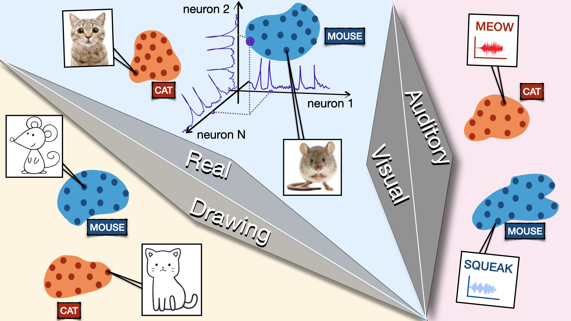
Figure 1: Neural manifolds are composed by the collection of the neural responses elicited by the same concept, either “cat” (red) or “mouse” (blue) in this illustration. These two concepts are expressed by different representations according to the different contexts: auditory or visual signals (stimulus modality as different contexts), realistic or cartoon-like images (visual styles as different contexts).

In this work, we develop a classification theory of non-linearly separable neural representations, that we model as correlated neural manifolds. Our contribution is twofold. First, we extend the existing geometric theory of capacity and abstraction to contextual and non-linear readouts. Second, we apply our theory to assess the nonlinear separability of representations in deep neural networks as a testbed for sensory hierarchy. Adding contexts enables more sophisticated classification rules by the readout, increasing the number of piece-wise linear components of the decision boundary. As a result, our framework quantitatively reveals that the layer hierarchy progressively untangles representations, as evidenced by a monotonic increase in capacity even in early layers, which was previously inaccessible to analysis Cohen et al. (2020). Furthermore, we find that capacity decreases when contexts are correlated. Importantly, our method is applicable to a wide range of datasets and models, both from machine learning and neural recordings, offering a unified approach to understand context-dependent computation in distributed representations across scales.
Theoretical framework.

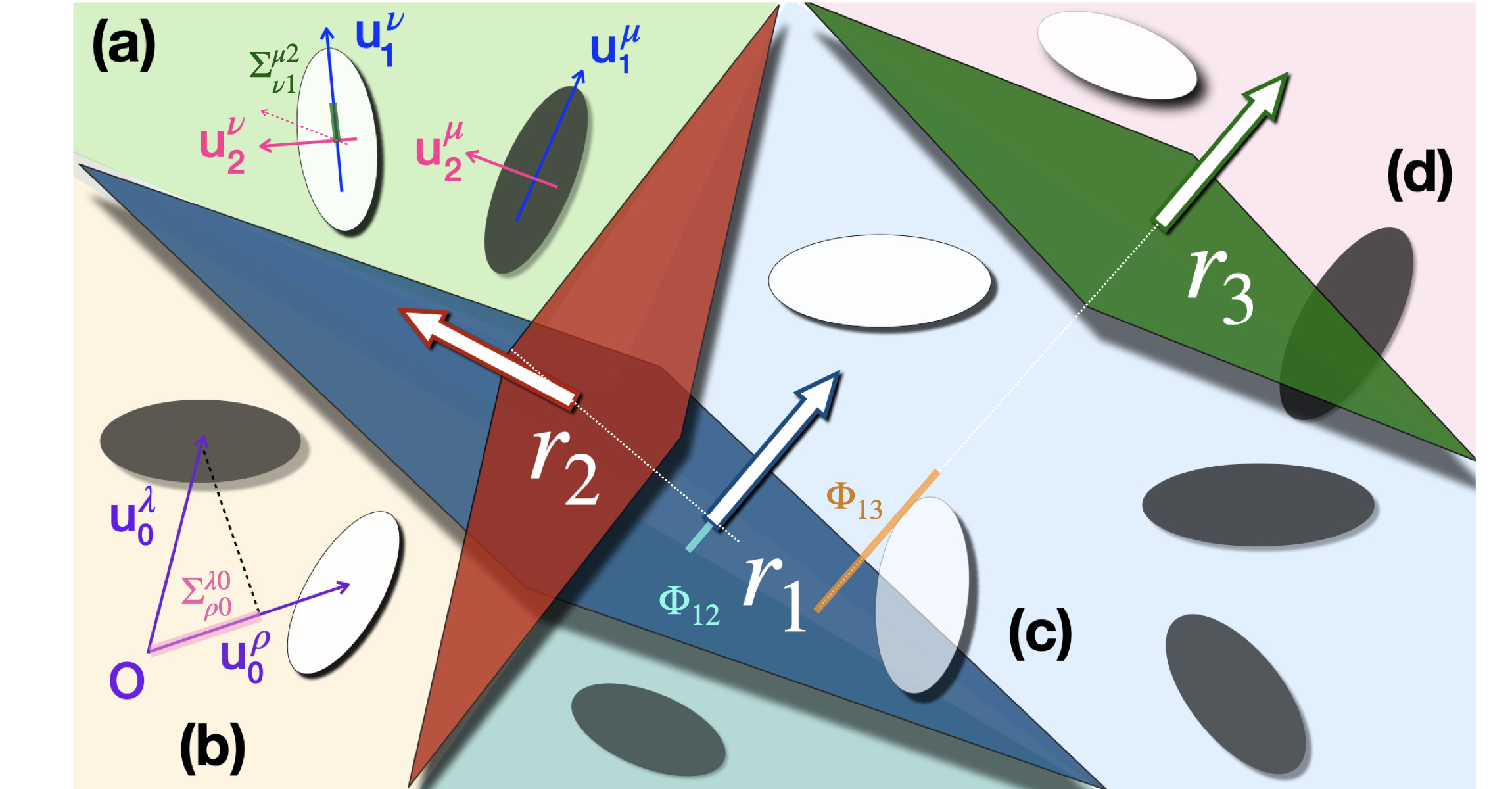
Figure 2: Three hyperplanes shatter the input space into different contexts, marked by different colors. Manifold shapes are ellipsoids, while labels are encoded by the black/white coloring. The vectors $\bm{r}_{1}$ and $\bm{r}_{2}$ define uncorrelated contexts ($\Phi_{12}\sim 0$), while $\bm{r}_{1}$ and $\bm{r}_{3}$ are highly correlated ($\Phi_{13}\sim 1$). (a) Correlations between manifold directions. (b) Correlation between manifold centers, where $\bf O$ denotes the origin. (c-d) Manifolds can be “cut” by context hyperplanes and lie into multiple contexts.

We model neural representations as low-dimensional manifolds embedded in high-dimensional space Chung et al. (2018). We consider manifolds $\mathcal{M}^{\mu}$, $\mu=1,\ldots,P$, each corresponding to a compact subset of an affine subspace of $\mathbb{R}^{N}$ with affine dimension $D\ll N$. A point on the manifold ${\bm{x}}^{\mu}\in\mathcal{M}^{\mu}$ can be parametrized as ${\bm{x}}^{\mu}({\bm{s}})={\bm{u}}^{\mu}_{0}+\sum_{i=1}^{D}s_{i}{\bm{u}}_{i}^{\mu}$, with ${\bm{s}}\in\mathcal{S}$. Here ${\bm{u}}^{\mu}_{0}$ denotes the center of the manifold, while $\{\bm{u}_{i}^{\mu}\}_{i=1}^{D}$ define a $D-$dimensional linear subspace containing the manifold, and the $D$ components $s_{i}$ are the coordinates of the point ${\bm{x}}^{\mu}$ on the manifold, constrained to a given shape by the set $\mathcal{S}$. We draw manifold directions $\bm{U}=\{{\bm{u}}_{0}^{\mu},\{{\bm{u}}_{i}^{\mu}\}_{i=1}^{D}\}_{\mu=1}^{P}$ from the joint probability distribution

$$p(\bm{U})\propto\exp\left(-\frac{N}{2}\sum_{\mu,\nu,i,j,l}(\bm{\Sigma}^{-1})^{\mu i}_{\nu j}u^{\mu}_{il}u^{\nu}_{jl}\right)\;,$$ (1)

where correlations between directions are encoded in the tensor $\bm{\Sigma}\in\mathbb{R}^{P(D+1)\times P(D+1)}$, as in Wakhloo et al. (2023). All points on a given manifold share the same label. Labels are binary and randomly assigned: $y^{\mu}=\pm 1$ with equal probability.
At variance with Chung et al. (2018); Wakhloo et al. (2023), we incorporate non-linear decisions to our classification rule by considering a neural network model with contextual information. The model we study is closely related to the recently proposed Gated Linear Networks Budden et al. (2020); Sezener et al. (2022); Veness et al. (2021): nonlinear neural architectures that remain analytically tractable Saxe et al. (2022); Li and Sompolinsky (2022). In particular, context switching is implemented by a gating mechanism based on half-space shattering with a set of context vectors ${\bm{r}}_{k}\in\mathbb{R}^{N}$, ${k=1,\ldots K}$. The network output is

$$f_{\bm{W}}({\bm{x}})=\sum_{{\bm{c}}\in\{0,1\}^{K}}g_{{\bm{c}}}\left(\{{\bm{x}}^{\top}{\bm{r}}_{k}\}_{k=1}^{K}\right)\,{{\bm{w}}_{\bm{c}}^{\top}{\bm{x}}}\;,$$ (2)

where ${\bm{x}}$ denotes the input, $\bm{W}=\{{\bm{w}}_{\bm{c}}\}_{{\bm{c}}\in\{0,1\}^{K}}$ are the trainable weights, each associated to a context ${\bm{c}}\in\{0,1\}^{K}$, and $g_{\bm{c}}$ are the gating functions. The label estimate is given by $\hat{y}={\rm sign}\left(f_{\bm{W}}({\bm{x}})\right)$. The gating functions shatter the input space into $2^{K}$ non-overlapping contexts, resulting from $K$ binary decisions implemented by the context hyperplanes: $g_{\bm{c}}(\{{\bm{x}}^{\top}{\bm{r}}_{k}\}_{k=1}^{K})=\prod_{k=1}^{K}\delta_{\Theta({\bm{r}}_{k}^{\top}{\bm{x}}),c_{k}}$, where $\delta_{i,j}$ denotes the Kronecker $\delta-$function and $\Theta$ the Heaviside step function, so that $g_{\bm{c}}(\{{\bm{x}}^{\top}{\bm{r}}_{k}\}_{k=1}^{K})=1$ if and only if ${\bm{x}}$ belongs to context ${\bm{c}}$, and zero otherwise. The context hyperplanes are fixed. Biases can be easily incorporated into the gating functions, but here we set them to zero for simplicity. Fig. 1 illustrates the advantage of contextual information in a non-linearly-separable classification task where representations of the same concept correspond to different sensory modalities or stylistic frameworks. The interplay of manifold and context geometry is schematized in Fig. 2.

A key quantity to assess the efficiency of neural representations is the manifold capacity, i.e., the maximal number of manifolds per dimension $\alpha=P/N$ that can be correctly classified by the nonlinear rule in Eq. (2) with high probability at a given margin $\gamma\geq 0$. In particular, we consider the thermodynamic limit $P,N\rightarrow\infty$, with $\alpha=\mathcal{O}_{N}(1)$. This corresponds to finding the largest $\alpha$ such that there exist a collection of decision hyperplanes $\bm{W}$, $\|{\bm{w}}_{\bm{c}}\|_{2}^{2}=N$ for all ${\bm{c}}\in\{0,1\}^{K}$, satisfying: $\min_{{\bm{x}}^{\mu}\in\mathcal{M}^{\mu}}y^{\mu}f_{\bm{W}}({\bm{x}}^{\mu})\geq\gamma$ for all $\mu=1,\ldots,P$ with probability one in the thermodynamic limit. This threshold can be determined by computing the average logarithm of the Gardner volume Gardner (1988) – the volume of the space of solutions – in the thermodynamic limit:

$$\begin{split}\overline{\ln V}=\overline{\underset{{\mathcal{S}(\sqrt{N})^{\otimes 2^{K}}}}{\int}\differential{\bm{W}}\prod_{\mu=1}^{P}\Theta\left(\min_{{\bm{x}}^{\mu}\in\mathcal{M}^{\mu}}y^{\mu}f_{\bm{W}}({\bm{x}}^{\mu})-\gamma\right)}\;,\end{split}$$ (3)

where $\mathcal{S}(\sqrt{N})$ is the $(N-1)-$dimensional hypersphere of radius $\sqrt{N}$ and the overbar denotes the average with respect to the labels ${\bm{y}}$ and the manifold directions $\bm{U}$.
Replica theory for nonlinear capacity. We compute the Gardner volume using the replica method Mézard et al. (1987); Monasson and Zecchina (1995); Baldassi et al. (2019); Zavatone-Veth and Pehlevan (2021). We defer the details of this computation to the supplemental material. We derive an exact formula for the storage capacity $\alpha^{*}$ for our model in the thermodynamic limit:

$$\begin{split}\frac{1}{\alpha^{*}(K,\bm{\Phi},\gamma)}=\\ \mathbb{E}_{{\bm{y},\bm{\xi},\bm{R}}}\left[\max_{{\bm{c}}\in\{0,1\}^{K}}\underset{{{\bm{H}}_{\bm{c}}\in\mathcal{H}^{\gamma}_{\bm{c}}({\bm{y}},{\bm{L}}|\bm{R})}}{\min}\displaystyle\;\frac{1}{P}\sum_{\mu=1}^{P}{\|\bm{H}^{\mu}_{{\bm{c}}}-{\bm{\xi}}^{\mu}_{\bm{c}}\|_{2}^{2}}\right].\end{split}$$ (4)

The capacity depends on the context correlations and the manifold statistics via the local fields ${H}^{\mu}_{i,{\bm{c}}}$, ${\xi}^{\mu}_{i,{\bm{c}}}$, and ${R}^{\mu}_{i,k}$; with $\mu=1,\ldots P$, $i=0,\ldots,D$, $k=1,\ldots,K$, and ${\bm{c}}\in\{0,1\}^{K}$. In particular, ${H}^{\mu}_{i,{\bm{c}}}$ represents the local field induced by the solution vector ${\bm{w}}_{\bm{c}}$ on the basis vector ${\bm{u}}^{\mu}_{i}$. Similarly, ${R}^{\mu}_{i,k}$ corresponds to the local field induced by the context-assignment vector ${\bm{r}}_{k}$ on the basis vector ${\bm{u}}^{\mu}_{i}$, and $\bm{R}^{\mu}_{i}\sim\mathcal{N}\left(\bm{0},\bm{\Phi}\right)$. The matrix $\bm{\Phi}\in\mathbb{R}^{K\times K}$ encodes the correlations between different context hyperplanes: $\Phi_{kk^{\prime}}={\bm{r}}_{k}^{\top}{\bm{r}}_{k^{\prime}}/N$, with the normalization $\|{\bm{r}}_{k}\|^{2}=N$ for all $k=1,\ldots,K$. The dependence of ${H}^{\mu}_{i,{\bm{c}}}$ on ${R}^{\nu}_{j,k}$ is hidden in the optimization constraint:

$$\begin{split}\mathcal{H}^{\gamma}_{\bm{c}}({\bm{y}},{\bm{L}}|\bm{R})=\Big{\{}\bm{H}_{\bm{c}}\in\mathbb{R}^{P\times(D+1)}\;:\;\forall\mu=1,\ldots,P\\ \min_{{\bm{s}}^{\mu}_{\bm{c}}\in\mathcal{S}\cap\mathcal{C}_{{\bm{c}}|{\bm{L}}^{\mu}\bm{R}}}y^{\mu}\sum_{\mu^{\prime},i^{\prime}}L^{\mu i}_{\mu^{\prime}i^{\prime}}H^{\mu^{\prime}}_{i^{\prime},{\bm{c}}}s^{\mu}_{i}\geq\gamma\Big{\}}\;,\end{split}$$ (5)

where $\bm{L}$ denotes the Cholesky decomposition of the manifold correlation tensor $\bm{\Sigma}$, satisfying: $\sum_{\rho,l}L^{\mu i}_{\rho,l}L^{\nu j}_{\rho,l}=\Sigma^{\mu,i}_{\nu,j}$. For each context ${\bm{c}}$, the manifold coordinates ${\bm{s}}^{\mu}$ are constrained to lie on an effective context, denoted by $\mathcal{C}_{{\bm{c}}|{\bm{L}}^{\mu}\bm{R}}=\{{\bm{s}}^{\mu}\in\mathbb{R}^{D+1}:\prod_{k=1}^{K}\delta_{\Theta({{\bm{s}}^{\mu}}^{\top}{\bm{L}}^{\mu}\bm{R}_{k}),c_{k}}=1\}$, where we have used the shorthand notation ${\bm{L}}^{\mu}\bm{R}\in\mathbb{R}^{K\times(D+1)}$ to indicate the matrix whose $(k,i)$ entry is ${\bm{L}}^{\mu i}\bm{R}_{k}=\sum_{\mu^{\prime},i^{\prime}}L^{\mu i}_{\mu^{\prime}i^{\prime}}\bm{R}^{\mu^{\prime}}_{k,i^{\prime}}$. Finally, the Gaussian variable ${\xi}_{i,{\bm{c}}}^{\mu}\sim\mathcal{N}(0,1)$ encodes the part of the variability in ${H}^{\mu}_{i,{\bm{c}}}$ due to quenched variability in the basis vector ${\bm{u}}^{\mu}_{i}$.

In summary, context dependence introduces additional constraints into the optimization problem, coupling the manifold geometry to the structure of the context hyperplanes. We test the validity of our theory on a synthetic dataset of isotropic Gaussian manifolds. Fig. S1 of the supplemental material shows our theoretical prediction for the capacity for different manifold correlations and number of contexts. We find a good agreement between theory and experiments. More details are discussed in the supplemental material.

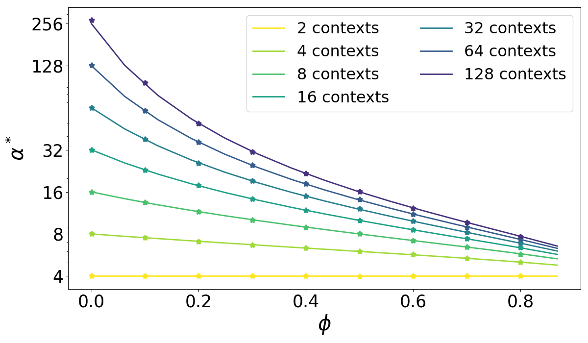
Figure 3: Capacity as a function of the context correlation parameter $\phi$ in the case of uncorrelated random points. Curves for different number of contexts are depicted with different colors. Full lines mark our theoretical predictions from Eq. (6), while symbols represent numerical simulations.

Special case: random points. We now turn to the simplest scenario of random points, i.e., $D=0$ and no manifold correlations, which proves useful for developing intuition on the problem. In particular, we take the context correlation matrix $\bm{\Phi}=(1-\phi)\bm{I}_{K}+\phi\mathbf{1}_{K}\mathbf{1}_{K}^{\top}$, where $\mathbf{1}_{K}$ denotes the $K-$dimensional vector with all entries equal to one. This choice allows to control context correlations tuning just one parameter $\phi\in[0,1]$. In this special case, the capacity formula reduces to

$$\begin{split}\frac{1}{\alpha^{*}(K,\phi,\gamma)}=\frac{(1+\gamma^{2})}{2^{K+1}}\\ \times\underset{{\bm{c}}\in\{0,1\}^{K}}{\max}\mathbb{E}_{\eta}\left[\prod_{k=1}^{K}\left[1+(1-2c_{k})\erf\left(\frac{\sqrt{\phi}\eta}{\sqrt{2(1-\phi)}}\right)\right]\right],\end{split}$$ (6)

with $\eta\sim\mathcal{N}(0,1)$. The details of this computation can be found in the supplemental material. In this prototypical setting, we find analytically that the capacity grows at most linearly with the number of contexts, and the maximal capacity $\alpha^{*}|_{\gamma=0}=2^{K+1}$ is achieved at $\phi=0$, i.e., orthogonal contexts, as a generalization of the classical result in the absence of contexts: $\alpha^{*}|_{\gamma=0}=2$ derived by Cover Cover (1965). This finding aligns with the experimental observation that orthogonal brain representations support efficient coding Flesch et al. (2022); Nogueira et al. (2023). From an “efficient coding” perspective, enhanced capacity at low context correlations may result from the optimal tiling of the input space with contexts when stimuli exhibit minimal structure. This phenomenon is related to the long-standing idea that the statistics of stimuli shape the distribution of receptive fields David et al. (2004) to achieve coding efficiency Doi et al. (2012). However, while prior work on efficient coding has focused on minimizing the loss of information, here we reframe the problem in terms of the task efficiency and capacity of the readout. Understanding how this picture is affected by introducing correlations between manifolds and contexts is an important direction for future work. Fig. 3 depicts the theoretical predictions from Eq. (6) (full lines) and the numerical estimates (symbols) of the capacity as a function of the context correlation $\phi$, for increasing number of contexts. We find excellent agreement between theory and simulations.

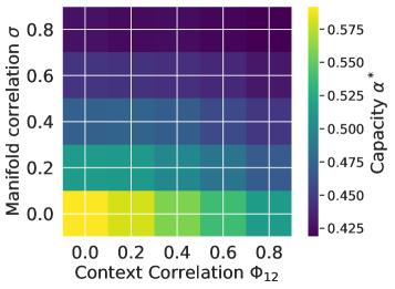
Figure 4: Capacity from Eq. (4) for spherical synthetic manifolds of latent dimension $D=10$, embedded in ambient dimension $N=8000$, different combinations of uniform manifold and context correlations $(\sigma,\Phi_{12})$, and four contexts.

Analysis of synthetic neural manifolds. We then turn to the case of synthetic data and investigate how the interplay of manifold and context correlations affect the capacity. We consider four contexts, i.e., $K=2$ context hyperplanes, so that context correlations are determined by one scalar off-diagonal term $\Phi_{12}$ of the correlation matrix. We draw spherical synthetic manifolds of latent dimension $D=10$ from the model in Eq. (1). For better visibility, we take normalized diagonal and constant off-diagonal correlations: $\Sigma^{\mu i}_{\mu i}=1$, $\Sigma^{\mu i}_{\nu j}=\sigma$ for all $(\mu,i)\neq(\nu,j)$. Fig. 4 displays the values of the capacity from Eq. (4) for a range of $\Phi_{12}$ and $\sigma$. We find that the capacity is decreasing both in manifold and context correlations. In particular, increasing the manifold correlations $\sigma$ has a dramatic impact in the capacity drop. It would be interesting to explore whether these trends change when context assignment is optimized to maximize capacity. We leave this extension to future work.
Analysis of ImageNet representations. We next apply our theoretical framework to quantify the capacity of neural representations in deep neural networks. We carry out experiments on Resnet-50 He et al. (2016) pretrained on ImageNet with supervised objective. We consider 50 image classes, randomly selected, and draw 50 images for each class to form neural manifolds, following the procedure in Cohen et al. (2020). For simplicity, we consider random context hyperplanes with no correlations ($\bm{\Phi}=\bm{I}_{K}$). We compute the capacity using the replica formula and validate the results through simulations, as in Stephenson et al. (2021). Concretely, the simulated capacity is estimated via a binary search (on the number of units and the number of manifolds) for the critical load of information. We provide more details on the numerical implementation of the experiments in the supplemental material. Fig. 5 displays the capacity as a function of the layer depth for different number of contexts $2^{K}=1,2,4,8,16$. The specific layers at which we capture the representations are indicated on the $x-$axis. The full lines mark our theoretical prediction from Eq. (4) while the symbols mark the numerical simulations. Even in the simplest case of orthogonal contexts, we find that our framework can quantify the progressive disentanglement of representations across layers, while the capacity curve in the absence of contexts ($K=0$) remains flat. Interestingly, with enough contexts, we can capture that capacity increases also at early layers. This phenomenon could not be captured by the context-less linear capacity theory Chung and Abbott (2021).

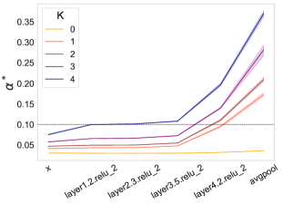
Figure 5: Capacity as a function of layer depth in Resnet-50 pretrained on ImageNet, for different number of contexts $2^{K}=1,2,4,8,16$ and orthogonal context hyperplanes. The $x-$axis displays the names of the network layers.

The number of contexts required to achieve a given capacity approximates the number of piece-wise linear components of the decision boundary, hence it is an indirect measure of the complexity of the representation. If we set, e.g., $\alpha=0.1$ (as marked by the horizontal dashed line in Fig. 5) we find that the readout layer can achieve this separability threshold with only $2$ contexts, while this number increases going back to the representations in the first hidden layer that requires $16$ contexts to be shattered. This observation clearly quantifies the generally accepted understanding that subsequent layers disentangle representations linearizing the decision boundary.
Discussion. We have adopted context-dependence as a unifying lens to study the efficiency of neural representations for complex tasks. In particular, we have proposed an analytically-solvable model that incorporates contextual information into classification, allowing for nonlinear decision boundaries. The decision-making rule is implemented by a collection of input-dependent “expert” neurons, each associated with distinct contexts through half-space gating mechanisms. First, we have derived an analytic expression for the manifold capacity. This formula elucidates the interplay between stimulus statistics and correlations within context hyperplanes. Furthermore, it enables probing the manifold capacity for non-linear readouts via piece-wise linear decision boundaries. Applications to both synthetic examples and artificial neural networks demonstrate the validity of our theoretical predictions. Our theory allows to explore the structure of memorization across layers of deep neural networks, capturing nonlinear disentanglement of representations.
The framework presented here paves the way for various further investigations. From a theoretical perspective, a natural extension of this work involves developing learning algorithms able to find high capacity context assignments. The interplay between context and manifold geometry can be further explored by explicitly introducing correlations with context hyperplanes in the manifold structure. In particular, it would be interesting to explore how contextual information impacts the classification of hierarchical data structures.
On the applications side, we plan to leverage our theory to test the efficiency of neural representations from biological datasets. To this end, it would be relevant to extend the analysis of Chou et al. (2024) by deriving effective geometric measures for manifold capacity with contexts. This extension would allow a systematic application of our theory to large-scale neural recordings. While in this paper we focus on contextual information gated from the input stimuli side, there have been lines of works studying contextual readout, e.g., multi-tasking in cognitive control Musslick et al. (2017). Extending our theory to unify the role of contextual information in both input and output can enhance our understanding of how neural representations efficiently accommodate complicated tasks.
Acknowledgments. We thank Will Slatton for useful feedback on this manuscript. This work was funded by the Center for Computational Neuroscience at the Flatiron Institute of the Simons Foundation and the Klingenstein-Simons Award to S.C. All experiments were performed on the Flatiron Institute high-performance computing cluster. F.M. was supported by he Human Frontiers Science Program and the Simons Foundation (Award Number: 1141576).

Appendix A Supplemental Material

A.1 Derivation of the Gardner volume via the replica method

In this section, we provide additional details on the derivation of the capacity threshold using the replica method Gardner (1988); Mézard et al. (1987). We use the replica trick to compute the log-volume averaged over the manifold directions $\bm{U}=\{\bm{u}_{i}^{\mu}\}_{i=0,\ldots,D}^{\mu=1,\ldots,P}$ and the labels ${\bm{y}}=\{y^{\mu}\}_{\mu=1}^{P}$. We denote this average by an overbar: $\overline{\ln Z}=\lim_{n\rightarrow 0^{+}}\left(\overline{Z^{n}}-1\right)/n$. The averaged $n^{\rm th}$ moment of the partition function is

$$\begin{split}\overline{Z^{n}}=\mathbb{E}_{{\bm{U}},{\bm{y}}}\left[\int\left(\prod_{a=1}^{n}\prod_{{\bm{c}}\in\{0,1\}^{K}}\differential{\bm{w}}^{a}_{\bm{c}}\;\delta\left(N-\|{\bm{w}}^{a}_{m}\|_{2}^{2}\right)\right)\left[\prod_{\mu=1}^{P}\prod_{{\bm{c}}\in\{0,1\}^{K}}\Theta\left(J^{({\bm{c}})}_{\mathcal{S}}({\bm{H}}^{\mu,a},\bm{R}^{\mu})-\gamma\right)\right]\right]\;,\end{split}$$ (S1)

where we have used the definitions

$$H^{\mu,a}_{i,{\bm{c}}}\coloneqq y^{\mu}\frac{{{\bm{w}}^{a}_{\bm{c}}}^{\top}{\bm{u}}_{i}^{\mu}}{\sqrt{N}}\;, R^{\mu}_{i,k}\coloneqq\frac{{{\bm{r}}_{k}}^{\top}{\bm{u}}^{\mu}_{i}}{\sqrt{N}}\;,$$ (S2)

while the function $J^{({\bm{c}})}_{\mathcal{S}}$ encodes the optimization constraints

$$J^{({\bm{c}})}_{\mathcal{S}}({\bm{H}},\bm{R})\coloneqq\begin{cases}H_{0,{\bm{c}}}+\underset{\bm{s}\in\mathcal{S}\cap C_{{\bm{c}}|\bm{R}}}{\min}\left\{{{\bm{H}}_{\bm{c}}}^{\top}{\bm{s}}\right\}&\text{if }\mathcal{S}\cap C_{{\bm{c}}|\bm{R}}\neq\emptyset\\ \bar{J}>\gamma&\text{if }\mathcal{S}\cap C_{{\bm{c}}|\bm{R}}=\emptyset\end{cases}\;,$$ (S3)

and we remind that $\mathcal{C}_{{\bm{c}}|\bm{R}}$ is defined such that ${\bm{s}}\in\mathcal{C}_{{\bm{c}}|\bm{R}}\;\;\Leftrightarrow\;\;\prod_{k=1}^{K}\Theta\left((-1)^{c_{k}}\left(R_{0,k}+{{\bm{s}}}^{\top}\bm{R}_{k}\right)\right)=1$. Here the constant $\bar{J}$ is introduced to ensure that the $\Theta$-function is $1$ when $\mathcal{S}\cap C_{{\bm{c}}|\bm{R}}=\emptyset$. We can introduce the auxiliary variables defined in Eq. (S2) via the Fourier transform of the Dirac $\delta-$function:

$$\begin{split}\overline{Z^{n}}=\int\left(\prod_{a=1}^{n}\prod_{{\bm{c}}\in\{0,1\}^{K}}\differential{\bm{w}}^{a}_{\bm{c}}\;\delta\left(N-\|{\bm{w}}^{a}_{\bm{c}}\|_{2}^{2}\right)\right)\\ \times\mathbb{E}_{\bm{U},{\bm{y}}}\left[\prod_{\mu=1}^{P}\int\mathcal{D}\bm{R}^{\mu}\prod_{a=1}^{n}\mathcal{D}{\bm{H}}^{\mu,a}\prod_{i=0}^{D}\left[\prod_{{\bm{c}}\in\{0,1\}^{K}}\sqrt{2\pi}\;\delta\left(H^{\mu,a}_{i,{\bm{c}}}-y^{\mu}\frac{{{\bm{w}}^{a}_{\bm{c}}}^{\top}{\bm{u}}_{i}^{\mu}}{\sqrt{N}}\right)\right]\left[\prod_{k=1}^{K}\sqrt{2\pi}\;\delta\left(R^{\mu}_{i,k}-\frac{{\bm{r}}_{k}^{\top}{\bm{u}}^{\mu}_{i}}{\sqrt{N}}\right)\right]\right],\end{split}$$ (S4)

and

$$\mathcal{D}\bm{R}^{\mu}\prod_{a=1}^{n}\mathcal{D}{\bm{H}}^{\mu,a}\coloneqq\left[\prod_{i=0}^{D}\left(\prod_{k=1}^{K}\frac{\differential R^{\mu}_{i,k}}{\sqrt{2\pi}}\right)\left(\prod_{a=1}^{n}\prod_{{\bm{c}}\in\{0,1\}^{K}}\frac{\differential H^{\mu,a}_{i,{\bm{c}}}}{\sqrt{2\pi}}\right)\right]\prod_{a=1}^{n}\prod_{{\bm{c}}\in\{0,1\}^{K}}\Theta\left(J^{({\bm{c}})}_{\mathcal{S}}({\bm{H}}^{\mu,a},\bm{R}^{\mu})-\gamma\right)\;.$$ (S5)

We assume that the vectors defining the manifold directions are drawn from the multivariate Gaussian distribution in Eq. (1) of the main text. Hence the variables ${\bm{H}}^{\mu,a}$ and $\bm{R}^{\mu}$ are Gaussian, with zero mean and covariance

$$\mathbb{E}_{\bm{U}}\left[H^{\mu,a}_{i,{\bm{c}}}H^{\nu,a^{\prime}}_{j,{\bm{c}}^{\prime}}\right]=y^{\mu}y^{\nu}Q^{aa^{\prime}}_{{\bm{c}}{\bm{c}}^{\prime}}\Sigma^{\mu i}_{\nu j}\;, \mathbb{E}_{\bm{U}}\left[H^{\mu,a}_{i,{\bm{c}}}R^{\nu}_{j,k}\right]=y^{\mu}\rho^{a}_{{\bm{c}},k}\Sigma^{\mu i}_{\nu j}\;, \mathbb{E}_{\bm{U}}\left[R^{\mu}_{i,k}R^{\nu}_{j,k^{\prime}}\right]=\Phi_{kk^{\prime}}\Sigma^{\mu i}_{\nu j}\;,$$ (S6)

where we have defined the overlap parameters

$$Q^{aa^{\prime}}_{{\bm{c}}{\bm{c}}^{\prime}}\coloneqq\frac{{{\bm{w}}^{a}_{\bm{c}}}^{\top}{\bm{w}}_{{\bm{c}}^{\prime}}^{a^{\prime}}}{N}\;, Q^{aa}_{{\bm{c}}{\bm{c}}}=1\;, \rho^{a}_{{\bm{c}},k}\coloneqq\frac{{{\bm{w}}^{a}_{\bm{c}}}^{\top}{\bm{r}}_{k}}{N}\;, \Phi_{kk^{\prime}}\coloneqq\frac{{\bm{r}}_{k}^{\top}{\bm{r}}_{k^{\prime}}}{{N}}\;.$$ (S7)

We can introduce these definitions via Dirac $\delta-$functions and compute the integrals over the weights. The average partition function to the $n^{\rm th}$ power can be rewritten as

$$\begin{split}\overline{Z^{n}}\propto\int\differential\bm{Q}\,\differential\bm{\rho}\,{\rm e}^{\frac{N}{2}\ln\det\left(\bm{Q}-\sum_{k,k^{\prime}}\Phi_{kk^{\prime}}^{-1}\bm{\rho}_{k}\bm{\rho}_{k^{\prime}}^{\top}\right)+\ln\mathcal{Z}}=\int\differential\bm{Q}\,\differential\bm{\rho}\,{\rm e}^{S(\bm{Q},\bm{\rho})}\;,\end{split}$$ (S8)

where

$$\mathcal{Z}=\int\left[\prod_{\mu=1}^{P}\mathcal{D}\bm{R}^{\mu}\prod_{a=1}^{n}\mathcal{D}\bm{H}^{\mu,a}\right]\exp\left(-\frac{1}{2}\sum_{\mu,\nu,i,j}{\mathbb{H}_{\mu i}}^{\top}(\mathbb{C}^{-1}\otimes\mathbb{Q}^{-1})^{\mu i}_{\nu j}\,\mathbb{H}_{\nu j}-\frac{1}{2}\ln\det\left(\mathbb{C}\otimes\mathbb{Q}\right)\right)\;,$$ (S9)

and we have introduced the shorthand notation:

$$\mathbb{H}^{a,{\bm{c}},k}_{\mu i}=\left(\begin{array}[]{c}H^{\mu,a}_{i,{\bm{c}}}\\ R^{\mu}_{i,k}\end{array}\right)\;, \mathbb{C}^{\mu i}_{\nu j}=\left(\begin{array}[]{cccc}y^{\mu}y^{\nu}\Sigma^{\mu i}_{\nu j}&y^{\mu}\Sigma^{\mu i}_{\nu j}\\ y^{\nu}\Sigma^{\mu i}_{\nu j}&\Sigma^{\mu i}_{\nu j}\end{array}\right)\;, \mathbb{Q}^{a{\bm{c}}k}_{a^{\prime}{\bm{c}}^{\prime}k^{\prime}}=\left(\begin{array}[]{cccc}Q^{aa^{\prime}}_{{\bm{c}}{\bm{c}}^{\prime}}&\rho^{a^{\prime}}_{{\bm{c}}^{\prime},k^{\prime}}\\ \rho^{a}_{{\bm{c}},k}&\Phi_{kk^{\prime}}\end{array}\right)\;.$$ (S16)

Replica symmetric ansatz:

We assume the following replica symmetric (RS) ansatz Mézard et al. (1987)

$$Q^{aa}_{mm^{\prime}} =Q^{*}_{mm^{\prime}}\;,\qquad\forall a=1,\ldots,n\;,\qquad\forall m,m^{\prime}=1,\ldots M\;,$$ (S17)

$$Q^{aa^{\prime}}_{mm^{\prime}} =q_{mm^{\prime}}\;,\qquad\forall a\neq a^{\prime}\;,a,a^{\prime}=1,\ldots,n\;,\qquad\forall m,m^{\prime}=1,\ldots M\;,$$ (S18)

$$\rho^{a}_{m,k} =\rho_{m,k}\;,\qquad\forall a=1,\ldots n\;.$$ (S19)

with the additional normalization constraint: $Q^{*}_{mm}=1$. The RS assumption is motivated by the observation that within each context the solution space is convex, and contexts do not overlap. Notice that we do not assume symmetry between different contexts. We compute all the terms in the action $S(\bm{Q},\bm{\rho})$ in Eq. (S8) under the RS ansatz.

$$\begin{split}&\frac{1}{2}\ln\det\left(\bm{Q}-\sum_{k,k^{\prime}}\Phi^{-1}_{kk^{\prime}}\bm{\rho}_{k}\bm{\rho}_{k^{\prime}}^{\top}\right)=\frac{1}{2}\left[(n-1)\ln\det\left(\bm{Q}^{*}-\bm{q}\right)+\ln\det\left(\bm{Q}^{*}-\bm{q}+n\left(\bm{q}-\bm{\rho}^{\top}\Phi^{-1}\bm{\rho}\right)\right)\right].\end{split}$$ (S20)

The matrix $\mathbb{Q}$ and its inverse $\mathbb{Q}^{-1}$ have the same block structure

$$\mathbb{Q}=\left(\begin{array}[]{ccccc}\bm{Q}^{*}&\bm{q}&\ldots&\bm{q}&\bm{\rho}^{\top}\\ \bm{q}&\ddots&\bm{q}&\bm{q}&\bm{\rho}^{\top}\\ \bm{q}&\ldots&\bm{q}&\bm{Q}^{*}&\bm{\rho}^{\top}\\ \bm{\rho}&\bm{\rho}&\bm{\rho}&\bm{\rho}&\bm{\Phi}\end{array}\right)\;,\qquad\mathbb{Q}^{-1}=\left(\begin{array}[]{ccccc}\tilde{\bm{Q}}^{*}&\tilde{\bm{q}}&\ldots&\tilde{\bm{q}}&\tilde{\bm{\rho}}^{\top}\\ \tilde{\bm{q}}&\ddots&\tilde{\bm{q}}&\tilde{\bm{q}}&\tilde{\bm{\rho}}^{\top}\\ \tilde{\bm{q}}&\ldots&\tilde{\bm{q}}&\tilde{\bm{Q}}^{*}&\tilde{\bm{\rho}}^{\top}\\ \tilde{\bm{\rho}}&\tilde{\bm{\rho}}&\tilde{\bm{\rho}}&\tilde{\bm{\rho}}&\tilde{\bm{\Phi}}\end{array}\right)\;,$$ (S29)

and the inverse elements can be computed from the relation $\mathbb{Q}\mathbb{Q}^{-1}={\rm Id}$. We find the following relations

$$\begin{split}\tilde{\bm{Q}}^{*}&=\left(\bm{Q}^{*}-\bm{q}\right)^{-1}-\left(\bm{Q}^{*}+(n-1)\bm{q}\right)^{-1}\bm{q}\left(\bm{Q}^{*}-\bm{q}\right)^{-1}\\ &\quad+\left(\bm{Q}^{*}+(n-1)\bm{q}\right)^{-1}\bm{\rho}^{\top}\left(\bm{\Phi}-n\bm{\rho}\left(\bm{Q}^{*}+(n-1)\bm{q}\right)^{-1}\bm{\rho}^{\top}\right)^{-1}\bm{\rho}\left(\bm{Q}^{*}+(n-1)\bm{q}\right)^{-1}\;,\end{split}$$ (S30)

$$\tilde{\bm{q}} =\tilde{\bm{Q}}^{*}-\left(\bm{Q}^{*}-\bm{q}\right)^{-1}\;,$$ (S31)

$$\tilde{\bm{\rho}} =-\left(\bm{\Phi}-n\bm{\rho}\left(\bm{Q}^{*}+(n-1)\bm{q}\right)^{-1}\bm{\rho}^{\top}\right)^{-1}\bm{\rho}\left(\bm{Q}^{*}+(n-1)\bm{q}\right)^{-1}\;,$$ (S32)

$$\tilde{\bm{\Phi}} =\left(\bm{\Phi}-n\bm{\rho}\left(\bm{Q}^{*}+(n-1)\bm{q}\right)^{-1}\bm{\rho}^{\top}\right)^{-1}\;.$$ (S33)

We then consider the Cholesky decomposition of the correlation matrix $\bm{\Sigma}$, that satisfies $\sum_{\mu^{\prime},i^{\prime}}L^{\mu i}_{\mu^{\prime}i^{\prime}}L^{\mu^{\prime}i^{\prime}}_{\nu j}=\Sigma^{\mu i}_{\nu j}$. It is useful to perform the rotations $H^{\mu,a}_{i,{\bm{c}}}\rightarrow y^{\mu}\sum_{\mu^{\prime},i^{\prime}}L^{\mu i}_{\mu^{\prime}i^{\prime}}H^{\mu^{\prime},a}_{i^{\prime},{\bm{c}}}$ and $R^{\mu}_{i,k}\rightarrow\sum_{\mu^{\prime},i^{\prime}}L^{\mu i}_{\mu^{\prime}i^{\prime}}R^{\mu^{\prime}}_{i^{\prime},k}$. This transformation allows us to decouple the indices $(\mu,i)$ in the Gaussian weight, coupling them in the constraint functions $J^{({\bm{c}})}_{\mathcal{S}}$. We find

$$\mathcal{Z}=\int\left[\prod_{\mu=1}^{P}\mathcal{D}\bm{R}^{\mu}\prod_{a=1}^{n}\mathcal{D}\bm{H}^{\mu,a}\right]\exp\left(-\frac{1}{2}\sum_{\mu,i}{\mathbb{H}_{\mu i}}^{\top}\mathbb{Q}^{-1}\mathbb{H}_{\mu i}-\frac{\alpha N}{2}\ln\det\mathbb{Q}\right)\;,$$ (S34)

where we have now changed the definition

$$\mathcal{D}\bm{R}^{\mu}\prod_{a=1}^{n}\mathcal{D}\bm{H}^{\mu,a}\coloneqq\left[\prod_{i=0}^{D}\left(\prod_{k=1}^{K}\frac{\differential R^{\mu}_{i,k}}{\sqrt{2\pi}}\right)\left(\prod_{a=1}^{n}\prod_{{\bm{c}}\in\{0,1\}^{K}}\frac{\differential H^{\mu,a}_{i,{\bm{c}}}}{\sqrt{2\pi}}\right)\right]\prod_{a=1}^{n}\prod_{{\bm{c}}\in\{0,1\}^{K}}\Theta\left(J^{({\bm{c}})}_{\mathcal{S}}(y^{\mu}{\bm{L}}^{\mu}{\bm{H}}^{a},{\bm{L}}^{\mu}\bm{R})-\gamma\right)\;,$$ (S35)

and we have used the shorthand notation ${\bm{L}}^{\mu}\bm{R}\in\mathbb{R}^{K\times(D+1)}$ to indicate the matrix whose $(k,i)$ entry is ${\bm{L}}^{\mu i}\bm{R}_{k}=\sum_{\mu^{\prime},i^{\prime}}L^{\mu i}_{\mu^{\prime}i^{\prime}}\bm{R}^{\mu^{\prime}}_{k,i^{\prime}}$. Upon exchanging the limits $n\rightarrow 0^{+}$ and $N\rightarrow\infty$, we find that the high dimensional limit of the log-volume density can be computed via saddle point method:

$$\begin{split}\frac{\overline{\ln Z}}{N}\underset{N\gg 1}{\;\longrightarrow\;}\underset{\bm{Q^{*}},\bm{q},\bm{\rho}}{\text{extr}}\;S_{\rm RS}(\bm{Q^{*}},\bm{q},\bm{\rho})\;,\end{split}$$ (S36)

where

$$S_{\rm RS}(\bm{Q^{*}},\bm{q},\bm{\rho}) =\frac{1}{2}\left[\ln\det(\bm{Q^{*}}-\bm{q})+{\rm Tr}\left((\bm{Q^{*}}-\bm{q})^{-1}\left(\bm{q}-\bm{\rho}^{\top}\bm{\Phi}^{-1}\bm{\rho}\right)\right)\right]$$ (S37)

$$\quad+\alpha\mathbb{E}_{{\bm{y}},\bm{\xi},\bm{R}}\left[\frac{1}{P}\ln\mathbb{E}_{\bm{H}}\left[\prod_{\mu=1}^{P}\prod_{{\bm{c}}\in\{0,1\}^{K}}\Theta(J^{({\bm{c}})}_{\mathcal{S}}(y^{\mu}{\bm{L}}^{\mu}{\bm{H}}^{a},{\bm{L}}^{\mu}\bm{R})-\gamma)\right]\right],$$ (S38)

and the averages are over $\bm{\xi}^{\mu}_{i}\sim\mathcal{N}(0,I_{M})$, $\bm{R}^{\mu}_{i}\leavevmode\nobreak\ \sim\leavevmode\nobreak\ \mathcal{N}\left(\bm{\rho}\bm{q}^{-1/2}\bm{\xi}^{\mu}_{i},\bm{\Phi}-\bm{\rho}^{\top}\bm{q}^{-1}\bm{\rho}^{\top}\right)$, and $\bm{H}^{\mu}_{i}\sim\mathcal{N}\left(\bm{q}^{1/2}\bm{\xi}^{\mu}_{i},\bm{\bm{Q}^{*}-\bm{q}}\right)$.

The main additional technical difficulty in our analysis, compared to previous related works Chung et al. (2018); Wakhloo et al. (2023), is that for more than one context the asymptotic closed-form formulas at a generic $\alpha$ are provided in terms of a set of coupled self-consistent saddle-point equations on $2^{K}\times 2^{K}$ and $K\times 2^{K}$ dimensional matrix order parameters, instead of just one scalar order parameter. This poses some challenges on the numerical evaluation of the solution, as previously pointed out in the context of learning problems Aubin et al. (2018); Loureiro et al. (2021); Cornacchia et al. (2023). We overcome these difficulties leveraging the simplifications of the formulas when evaluated at capacity $\alpha=\alpha^{*}$ and exploiting the structure of the solution space to make useful assumptions on the order parameters.

The structure of the solution space with non-overlapping contexts.

Given that contexts are non overlapping, each solution $\{{\bm{w}}_{\bm{c}}\}_{{\bm{c}}\in\{0,1\}^{K}}\in\mathcal{W}$ is the union of solutions across contexts $\mathcal{W}=\mathcal{W}_{1}\times\mathcal{W}_{2}\times\ldots\times\mathcal{W}_{2^{K}}$. This implies $Q^{*}_{{\bm{c}}{\bm{c}}^{\prime}}=q_{{\bm{c}}{\bm{c}}^{\prime}}$ for all ${\bm{c}}\neq{\bm{c}}^{\prime}$ and at every $\alpha$. Therefore, when contexts do not overlap, the covariance $(\bm{Q}^{*}-\bm{q})$ of the ${\bm{H}}-$fields is diagonal, with entries $(1-q_{{\bm{c}}{\bm{c}}})$. Moreover, due to the random labeling and the absence of context overlap and context-manifold correlations, it is reasonable to assume $q_{{\bm{c}}{\bm{c}}^{\prime}}=0$ for all ${\bm{c}}\neq{\bm{c}}^{\prime}$ and $\bm{\rho}=\bm{0}$. These observations imply that the ${\bm{H}}-$fields are effectively uncorrelated across contexts, hence we can factorize the expectation and write

$$\begin{split}\ln\mathbb{E}_{\bm{H}}\left[\prod_{\mu=1}^{P}\prod_{{\bm{c}}\in\{0,1\}^{K}}\Theta(J^{({\bm{c}})}_{\mathcal{S}}(y^{\mu}{\bm{L}}^{\mu}\bm{H}_{\bm{c}},\bm{R})-\gamma)\right]=\sum_{{\bm{c}}\in\{0,1\}^{K}}\ln\mathbb{E}_{{\bm{H}}_{\bm{c}}}\left[\prod_{\mu=1}^{P}\Theta(J^{({\bm{c}})}_{\mathcal{S}}(y^{\mu}{\bm{L}}^{\mu}\bm{H}_{\bm{c}},{\bm{L}}^{\mu}\bm{R})-\gamma)\right]\;.\end{split}$$ (S39)

We obtain

$$\begin{split}S_{RS}(\{{q}_{{\bm{c}}{\bm{c}}}\})&=\frac{1}{2}\sum_{{\bm{c}}\in\{0,1\}^{K}}\left[\ln\det(1-q_{{\bm{c}}{\bm{c}}})+\frac{{q}_{{\bm{c}}{\bm{c}}}}{1-q_{{\bm{c}}{\bm{c}}}}\right]\\ &\qquad+\alpha\mathbb{E}_{\bm{y},{\bm{\xi}},\bm{R}}\left[\frac{1}{P}\sum_{{\bm{c}}\in\{0,1\}^{K}}\ln\mathbb{E}_{{\bm{H}}_{\bm{c}}}\left[\prod_{\mu=1}^{P}\Theta(J^{({\bm{c}})}_{\mathcal{S}}(y^{\mu}{\bm{L}}^{\mu}\bm{H}_{\bm{c}},{\bm{L}}^{\mu}\bm{R})-\gamma)\right]\right]\;,\end{split}$$ (S40)

where averages are now over $\bm{\xi}^{\mu}_{i}\sim\mathcal{N}(0,I_{M})$, $\bm{R}^{\mu}_{i}\leavevmode\nobreak\ \sim\leavevmode\nobreak\ \mathcal{N}\left(\bm{0},\bm{\Phi}\right)$, and ${H}^{\mu}_{i,{\bm{c}}}\sim\mathcal{N}\left(\sqrt{{q}_{{\bm{c}}{\bm{c}}}}\,\xi^{\mu}_{i,{\bm{c}}}\,,\,{1-{q}_{{\bm{c}}{\bm{c}}}}\right)$.

A.2 General case: capacity for manifolds

We introduce an auxiliary function

$$\hat{S}_{\text{min}}=\frac{1}{2}\ln(1-q_{\tilde{\bm{c}}\tilde{\bm{c}}})+\frac{1}{2}\frac{q_{\tilde{\bm{c}}\tilde{\bm{c}}}}{1-q_{\tilde{\bm{c}}\tilde{\bm{c}}}}+\frac{\alpha}{P}\mathbb{E}_{\bm{y},{\bm{\xi}},\bm{R}}\left[\ln\mathbb{E}_{{\bm{H}}_{\tilde{\bm{c}}}}\left[\prod_{\mu=1}^{P}\Theta(J^{(\tilde{\bm{c}})}_{\mathcal{S}}(y^{\mu}{\bm{L}}^{\mu}\bm{H}_{\tilde{\bm{c}}},{\bm{L}}^{\mu}\bm{R})-\gamma)\right]\right],$$ (S41)

where $\tilde{\bm{c}}=\text{arg}\underset{{\bm{c}}\in\{0,1\}}{\text{min}}\frac{1}{P}\ln\mathbb{E}_{{\bm{H}}_{\bm{c}}}\left[\prod_{\mu=1}^{P}\Theta(J^{({\bm{c}})}_{\mathcal{S}}(y^{\mu}{\bm{L}}^{\mu}\bm{H}_{\bm{c}},{\bm{L}}^{\mu}\bm{R})-\gamma)\right]$. The function $\hat{S}_{\rm min}$ is a lower bound on the replica symmetric action $S_{\rm RS}$. Indeed, for each context $\tilde{\bm{c}}$:

$$\ln(1-q_{\tilde{\bm{c}}\tilde{\bm{c}}})+\frac{q_{\tilde{\bm{c}}\tilde{\bm{c}}}}{1-q_{\tilde{\bm{c}}\tilde{\bm{c}}}}\geq 0\;, \ln(1-q_{\tilde{\bm{c}}\tilde{\bm{c}}})+\frac{q_{\tilde{\bm{c}}\tilde{\bm{c}}}}{1-q_{\tilde{\bm{c}}\tilde{\bm{c}}}}\leq\sum_{{\bm{c}}\in\{0,1\}^{K}}\left[\ln(1-q_{{\bm{c}}{\bm{c}}})+\frac{q_{{\bm{c}}{\bm{c}}}}{1-q_{{\bm{c}}{\bm{c}}}}\right]\;.$$ (S42)

We also have that

$$\begin{split}2^{K}\lambda({\bm{y}},{\bm{\xi}},\bm{R})\leq\sum_{{\bm{c}}^{\prime}}\frac{1}{P}\ln\mathbb{E}_{{\bm{H}}_{{\bm{c}}^{\prime}}}\left[\prod_{\mu=1}^{P}\Theta(J^{({\bm{c}}^{\prime})}_{\mathcal{S}}(y^{\mu}{\bm{L}}^{\mu}\bm{H}_{{\bm{c}}^{\prime}},{\bm{L}}^{\mu}\bm{R})-\gamma)\right]\;,\end{split}$$ (S43)

where we have defined

$$\lambda({\bm{y}},{\bm{\xi}},\bm{R}) \coloneqq\underset{{\bm{c}}\in\{0,1\}}{\text{min}}\frac{1}{P}\ln\mathbb{E}_{{\bm{H}}_{{\bm{c}}}}\left[\prod_{\mu=1}^{P}\Theta(J^{({\bm{c}})}_{\mathcal{S}}(y^{\mu}{\bm{L}}^{\mu}\bm{H}_{\bm{c}},{\bm{L}}^{\mu}\bm{R})-\gamma)\right]\leq 0\;.$$ (S44)

Furthermore, due to the spherical constraint on the weight space, the log-volume density is bounded in the infinite-dimensional limit. Therefore, there exists a constant $\bar{s}$ such that

$$\hat{S}_{\rm min}+2^{K-1}\lambda({\bm{y}},{\bm{\xi}},\bm{R})\leq S_{\rm RS}\leq\hat{S}_{\rm min}+2^{K-1}\bar{s},$$ (S45)

and the phase transition at the capacity threshold $S_{\rm RS}\rightarrow-\infty$ is controlled by the divergence of $\hat{S}_{\rm min}$ to $-\infty$. From now on, the calculation follows the lines of Chung et al. (2018); Wakhloo et al. (2023). As $q_{\tilde{\bm{c}}\tilde{\bm{c}}}\rightarrow 1$ in Eq. (S41), at leading order we have

$$\ln(1-q_{\tilde{\bm{c}}\tilde{\bm{c}}})+\frac{{q}_{\tilde{\bm{c}}\tilde{\bm{c}}}}{1-q_{\tilde{\bm{c}}\tilde{\bm{c}}}}\;\underset{q_{\tilde{\bm{c}}\tilde{\bm{c}}}\rightarrow 1}{\simeq}\;\frac{1}{1-q_{\tilde{\bm{c}}\tilde{\bm{c}}}}\;,$$ (S46)

and

$$\frac{1}{P}\ln\mathbb{E}_{\bm{H}_{\tilde{\bm{c}}}}\left[\prod_{\mu=1}^{P}\Theta(J^{(\tilde{\bm{c}})}_{\mathcal{S}}(y^{\mu}{\bm{L}}^{\mu}\bm{H_{\tilde{\bm{c}}}},{\bm{L}}^{\mu}\bm{R})-\gamma)\right]\simeq-\frac{1}{2}\;\;\frac{\underset{{\bm{H}}_{\tilde{\bm{c}}}\in\mathcal{H}_{\tilde{\bm{c}}}^{\gamma}({\bm{y}},{\bm{L}}|\bm{R})}{\min}\displaystyle\frac{1}{P}\sum_{\mu=1}^{P}\|\bm{H}^{\mu}_{\tilde{\bm{c}}}-\bm{q}_{\tilde{\bm{c}}}^{1/2}{\bm{\xi}}^{\mu}\|_{2}^{2}}{1-q_{\tilde{\bm{c}}\tilde{\bm{c}}}}\;,$$ (S47)

where we have defined

$$\begin{split}\mathcal{H}^{\gamma}_{\bm{c}}({\bm{y}},{\bm{L}}|\bm{R})=\Big{\{}\bm{H}_{\bm{c}}\in\mathbb{R}^{P\times(D+1)}\;:\;\forall\mu=1,\ldots,P\;,\quad\min_{{\bm{s}}^{\mu}_{\bm{c}}\in\mathcal{S}\cap\mathcal{C}_{{\bm{c}}|{\bm{L}}^{\mu}\bm{R}}}y^{\mu}\sum_{\mu^{\prime},i^{\prime}}L^{\mu i}_{\mu^{\prime}i^{\prime}}H^{\mu^{\prime}}_{i^{\prime},{\bm{c}}}s^{\mu}_{i}\geq\gamma\Big{\}}\;.\end{split}$$ (S48)

Therefore, close to the transition, we have that

$$\hat{S}_{\rm min}\underset{q_{\tilde{\bm{c}}\tilde{\bm{c}}}\rightarrow 1}{\simeq}\frac{1}{2}\mathbb{E}_{{\bm{y}},{\bm{\xi}},\bm{R}}\left[\frac{1}{1-q_{\tilde{\bm{c}}\tilde{\bm{c}}}}\left(1-\alpha\underset{{\bm{H}}_{\tilde{\bm{c}}}\in\mathcal{H}({\bm{y}},{\bm{L}}|\bm{R})}{\min}\displaystyle\frac{1}{P}\sum_{\mu=1}^{P}\|\bm{H}^{\mu}_{\tilde{\bm{c}}}-{\bm{\xi}}^{\mu}\|_{2}^{2}\right)\right].$$ (S49)

The transition happens when the right hand side changes sign, which determines the capacity threshold

$$\frac{1}{\alpha^{*}(K,\bm{\Phi},\gamma)}=\mathbb{E}_{{\bm{y},\bm{\xi},\bm{R}}}\left[\max_{{\bm{c}}\in\{0,1\}^{K}}\underset{{{\bm{H}}_{\bm{c}}\in\mathcal{H}^{\gamma}_{\bm{c}}({\bm{y}},{\bm{L}}|\bm{R})}}{\min}\displaystyle\;\frac{1}{P}\sum_{\mu=1}^{P}{\|\bm{H}^{\mu}_{{\bm{c}}}-{\bm{\xi}}^{\mu}_{\bm{c}}\|_{2}^{2}}\right].$$ (S50)

Comparison to the context-less formula.

The capacity formula in Eq. (S50) is a generalization of the context-less capacity $\alpha^{*}_{\cancel{C}}$ for correlated neural manifolds derived in Eq. (5) of Wakhloo et al. (2023):

$$\frac{1}{\alpha^{*}_{\cancel{C}}(\gamma)}=\mathbb{E}_{{\bm{y},\bm{\xi},\bm{R}}}\left[\underset{{{\bm{H}}\in\mathcal{A}^{\gamma}({\bm{y}},{\bm{L}})}}{\min}\displaystyle\;\frac{1}{P}\sum_{\mu=1}^{P}{\|\bm{H}^{\mu}-{\bm{\xi}}^{\mu}\|_{2}^{2}}\right],$$ (S51)

where the fields are independent of contexts and the constraint only depends on the manifold shapes and correlations:

$$\mathcal{A}^{\gamma}({\bm{y}},{\bm{L}})=\Big{\{}\bm{H}\in\mathbb{R}^{P\times(D+1)}\;:\;\forall\mu=1,\ldots,P\;,\quad\min_{{\bm{s}}^{\mu}\in\mathcal{S}}y^{\mu}\sum_{\mu^{\prime},i^{\prime}}L^{\mu i}_{\mu^{\prime}i^{\prime}}H^{\mu^{\prime}}_{i^{\prime}}s^{\mu}_{i}\geq\gamma\Big{\}}\;.$$ (S52)

A.3 Special case: capacity for points

In the special case of random uncorrelated points, we have that $D=0$, $\Sigma^{\mu i}_{\nu j}=\delta_{\mu\nu}\delta_{ij}$ and we can set $y^{\mu}=1$ without loss of generality. Therefore, the average over ${\bm{H}}_{\bm{c}}$ in Eq. (S40) simplifies to

$$\begin{split}\frac{1}{P}\ln\mathbb{E}_{{\bm{H}}_{\bm{c}}}&\left[\prod_{\mu=1}^{P}\Theta(J^{({\bm{c}})}_{\mathcal{S}}(y^{\mu}{\bm{L}}^{\mu}\bm{H}_{\bm{c}},{\bm{L}}^{\mu}\bm{R})-\gamma)\right]=\\ &=\frac{1}{P}\left[\prod_{k=1}^{K}\Theta\left((-1)^{c_{k}}R_{k}\right)\right]\ln\left(\prod_{\mu=1}^{P}\int\frac{\differential H^{\mu}_{0,{\bm{c}}}\,{\rm e}^{-{\left(H^{\mu}_{0,{\bm{c}}}-\sqrt{q_{{\bm{c}}{\bm{c}}}}\xi^{\mu}_{0,{\bm{c}}}\right)^{2}}/{2(1-q_{{\bm{c}}{\bm{c}}})}}}{\sqrt{2\pi(1-q_{{\bm{c}}{\bm{c}}})}}\Theta\left(H^{\mu}_{0,{\bm{c}}}-\gamma\right)\right)\\ &=\left[\prod_{k=1}^{K}\Theta\left((-1)^{c_{k}}R_{k}\right)\right]\ln\left(\frac{1}{2}{\rm erfc}\left(\frac{\gamma-{\xi}_{\bm{c}}}{\sqrt{2\,(1-q_{{\bm{c}}{\bm{c}}})}}\right)\right)\;,\end{split}$$ (S53)

where in the last equation we have dropped the indices $\mu$ and $0$ from $\xi_{\bm{c}}\sim\mathcal{N}(0,1)$ for simplicity. It is useful to define the context probability

$$P({\bm{c}}|\bm{\Phi})=\mathbb{E}_{\bm{R}}\left[\prod_{k=1}^{K}\Theta\left((-1)^{c_{k}}R_{k}\right)\right]\in[0,1]\;,\qquad\bm{R}\sim\mathcal{N}(\bm{0},\bm{\Phi})\;.$$ (S54)

The replica-symmetric action in Eq. (S40) simplifies to

$$S_{\rm RS}=\frac{1}{2}\sum_{{\bm{c}}\in\{0,1\}^{K}}\left[\ln(1-q_{{\bm{c}}{\bm{c}}})+\frac{q_{{\bm{c}}{\bm{c}}}}{1-q_{{\bm{c}}{\bm{c}}}}\right]+\alpha\,\mathbb{E}_{{\xi}_{\bm{c}}}\left[\sum_{{\bm{c}}\in\{0,1\}^{K}}P({\bm{c}}|\bm{\Phi})\ln\left(\frac{1}{2}{\rm erfc}\left(\frac{\gamma-{\xi}_{\bm{c}}}{\sqrt{2\,(1-q_{{\bm{c}}{\bm{c}}})}}\right)\right)\right]\;.$$ (S55)

We can define the auxiliary function

$$\hat{S}_{\rm min}=\mathbb{E}_{\xi_{\tilde{\bm{c}}}}\left[\frac{1}{2}\left(\ln(1-q_{\tilde{\bm{c}}\tilde{\bm{c}}})+\frac{q_{\tilde{\bm{c}}\tilde{\bm{c}}}}{1-q_{\tilde{\bm{c}}\tilde{\bm{c}}}}\right)+\alpha P(\tilde{\bm{c}}|\bm{\Phi})\ln\left(\frac{1}{2}{\rm erfc}\left(\frac{\gamma-{\xi}_{\tilde{\bm{c}}}}{\sqrt{2\,(1-q_{\tilde{\bm{c}}\tilde{\bm{c}}})}}\right)\right)\right],$$ (S56)

where in this case $\tilde{\bm{c}}={\rm arg}\underset{{\bm{c}}\in\{0,1\}^{K}}{\min}P({\bm{c}}|\bm{\Phi})\ln\left(\frac{1}{2}{\rm erfc}\left(\frac{\gamma-{\xi}_{\bm{c}}}{\sqrt{2\,(1-q_{{\bm{c}}{\bm{c}}})}}\right)\right)$. The capacity transition can be obtained by a similar argument as for the manifold case, where

$$\ln\left(\frac{1}{2}{\rm erfc}\left(\frac{\gamma-{\xi}_{\tilde{\bm{c}}}}{\sqrt{2\,(1-q_{\tilde{\bm{c}}\tilde{\bm{c}}})}}\right)\right)\underset{q_{\tilde{\bm{c}}\tilde{\bm{c}}\rightarrow 1}}{\simeq}-\frac{\left(\gamma-{\xi}_{\tilde{\bm{c}}}\right)^{2}}{2(1-q_{\tilde{\bm{c}}\tilde{\bm{c}}})}\Theta(\gamma-\xi_{\tilde{\bm{c}}})\;.$$ (S57)

Uniform off-diagonal context correlations.

We consider a special case of context correlation matrix: $\bm{\Phi}=(1-\phi)\bm{I}_{K}+\phi\bm{1}_{K}\bm{1}_{K}^{\top}$, where $\bm{1}_{K}$ denotes the $K-$dimensional vector with all entries equal to one. Thus, we have that $\det\bm{\Phi}=(1-\phi)^{K-1}\left(1+(K-1)\phi\right)$ and $\bm{\Phi}^{-1}=(1-\phi)^{-1}\left(\bm{I}_{K}-\phi\bm{1}_{K}\bm{1}_{K}^{\top}/(1+\phi(K-1))\right)$ by Sherman-Morrison lemma. The context probability reduces to

$$\begin{split}P({\bm{c}}|\phi)&=\int\left[\prod_{k=1}^{K}\frac{\differential R_{k}}{\sqrt{2\pi(1-\phi)}}\,\Theta\left((-1)^{c_{k}}R_{k}\right)\right]\sqrt{\frac{1-\phi}{1+(K-1)\phi}}{\rm e}^{-\frac{\bm{R}^{\top}\bm{R}}{2(1-\phi)}+\frac{\phi(\bm{R}^{\top}\bm{1}_{K})^{2}}{2(1-\phi)\left(1+(K-1)\phi\right)}}\\ &=\sqrt{\frac{1-\phi}{1+(K-1)\phi}}\mathbb{E}_{\eta}\left[\prod_{k=1}^{K}\int\frac{\differential R_{k}}{\sqrt{2\pi(1-\phi)}}\,\Theta\left((-1)^{c_{k}}R_{k}\right){\rm e}^{-\frac{R_{k}^{2}}{2(1-\phi)}+\frac{\sqrt{\phi}\eta R_{k}}{\sqrt{(1-\phi)(1+(K-1)\phi)}}}\right]\\ &=\mathbb{E}_{\eta}\left[2^{-K}\prod_{k=1}^{K}\left[1+(1-2c_{k})\erf\left(\frac{\sqrt{\phi}\eta}{\sqrt{2(1-\phi)}}\right)\right]\right]\end{split}$$ (S58)

where $\eta\sim\mathcal{N}(0,1)$.

A.4 Details on the numerical estimation of replica formula

In the numerical experiments, a manifold is modeled as a point cloud. For simplicity, we focus on the case where every manifold has the same number of points. Let $N$ be the number of units, let $P$ be the number of manifolds, and let $M$ be the number of points per manifold. The $\mu$-th manifold $\mathcal{M}^{\mu}$ consists of a collection of points $\{x^{\mu}_{1},\dots,x^{\mu}_{M}\}$ where $x^{\mu}_{i}\in\mathbb{R}^{N}$ for each $i=1,\dots,M$. Without loss of generality, we assume points in the same manifold are linearly independent.

The algorithm that computes capacity consists of two steps: (1) compute the correlations between manifolds, (2) sample the quenched disorder and calculate the capacity. The following are the pseudocodes for each step. In the following algorithms, $A\leftarrow\{x_{i}\}$ denotes putting the collection of vectors $\{x_{i}\}$ on the rows of $A$.

Step 1: Compute the correlations between manifolds.

In this step we first compute the center of mass of each manifold $x_{0}^{\mu}$ and center each point as $\bar{x}_{i}^{\mu}=x_{i}^{\mu}-x_{0}^{\mu}$. Next, we find a basis for the centered points for each manifold and estimate the covariance tensor $C^{\mu,i}_{\nu,j}$ accordingly. This step is exactly the same as the corresponding step in Wakhloo et al. (2023); Chou et al. (2024). See Algorithm 1 for details.

Algorithm 1 Compute the correlations between manifolds

Input: $\{\mathcal{M}^{\mu}\}_{\mu=1}^{P}$: $P$ manifolds of $M$ points in an ambient dimension of $N$.

Output: $C:$ Correlation tensor of shape $P\times(M+1)\times P\times(M+1)$; $\{\tilde{\mathcal{M}}^{\mu}\}_{\mu=1}^{P}$: $P$ manifolds of $M$ points in an ambient dimension of $M+1$.

1:for $\mu$ from $1$ to $P$ do

2:     $x_{0}^{\mu}\leftarrow\frac{1}{M}\sum_{i}x_{i}^{\mu}$.

3:     $\bar{x}_{i}^{\mu}\leftarrow x_{i}^{\mu}-x_{0}^{\mu}$ for each $i=1,\dots,M$.

4:end for

5:for $\mu$ from $1$ to $P$ do

6:     $Q\leftarrow$ an orthogonal basis for $\textsf{span}(\{\bar{x}_{i}^{\mu}\})$

7:     $z^{\mu}_{i}\leftarrow Q^{\top}\bar{x}^{\mu}_{i}$ for each $i=1,\dots,M$.

8:     $\widetilde{\mathcal{M}}^{\mu}\leftarrow\{\tilde{x}^{\mu}_{i}\}_{i=1}^{M}$ where $\tilde{x}^{\mu}_{i}=[z^{\mu}_{i}\ 1]$.

9:     $q_{0}^{\mu}\leftarrow\bar{x}_{0}^{\mu}$.

10:     $q_{i}^{\mu}\leftarrow Q[i]$ for $i=1,\dots,M$.

11:end for

12:Let $C$ be the $P\times(M+1)\times P\times(M+1)$ tensor with $C^{\mu,i}_{\nu,j}=\langle q^{\mu}_{i},q^{\nu}_{j}\rangle$ for each $\mu,\nu\in\{1,\dots,P\}$ and $i,j\in\{0,1,\dots,M\}$.

13:return $C,\{\widetilde{\mathcal{M}}^{\mu}\}_{\mu=1}^{P}$.

Step 2: Sample the quenched disorder and calculate capacity.

In this step, we first sample $K$ context hyperplanes $\{\mathbf{R}_{k}\}_{k=1}^{K}$. Next, we conduct $n_{t}$ ($n_{t}=100$ in all experiments) repetition of random sampling $\xi,\{R_{k}\}$ for averaging. For each repetition, for each context we sample the manifold disorder and the create quadratic programming problem with the points that lie in the context (as defined by $\{R_{k}\}_{k=1}^{K}$). Finally, capacity is the inverse of the average of the maximum over the outcome of the quadratic programming problems. Note that when $K=0$ this step is exactly the same as the corresponding step in Wakhloo et al. (2023); Chou et al. (2024). See Algorithm 2 for details.

Algorithm 2 Sample the quenched disorder and calculate capacity

Input: $C:$ Correlation tensor of shape $P\times(M+1)\times P\times(M+1)$; $\{\widetilde{\mathcal{M}}^{\mu}\}_{\mu=1}^{P}$: $P$ manifolds of $M$ points in an ambient dimension of $M+1$; $n_{t}$: number of samples; $\kappa$: margin; $K$: number of context hyperplanes; $\psi$: correlation between a pair of context hyperplanes.

Output: $\alpha$: capacity.

1:Sample $\{\mathbf{R}_{k}\}_{k=1}^{K}$ where $\mathbf{R}_{k}\in\mathbb{R}^{P\times(M+1)}$ and the $i$-th entry of $\mathbf{R}_{k}$ jointly samples from the multivariate Gaussian distribution with mean $0$ and covariance $(1-\psi)\delta_{kk^{\prime}}+\psi$.

2:$\textsf{conv}(\{\widetilde{M}^{\mu}\})\leftarrow\cup_{\mu}\cup_{k}\left\{y+\frac{\mathbf{R}_{k}^{\top}y}{\mathbf{R}_{k}^{\top}(x-y)}(x-y):x,y\in\widetilde{M}^{\mu},\ \mathbf{R}_{k}^{\top}x\geq 0,\ \mathbf{R}_{k}^{\top}y\leq 0\right\}$.

3:for $\ell$ from $1$ to $n_{t}$ do

4:     for $b\in\{-1,1\}^{K}$ do

5:         $T_{k}\leftarrow$ a vector sampled from isotropic $P\times(M+1)$ dimensional Gaussians.

6:         $y\leftarrow$ a random vector from $\{1,-1\}^{P}$.

7:         $L\leftarrow\textsf{Cholesky}(C)$. $\triangleright$ Cholesky decomposition

8:         $A\leftarrow I_{P(M+1)}$.

9:         $q\leftarrow-T_{\ell}$.

10:         $G\leftarrow(y\odot L)\textsf{conv}(\{\widetilde{M}^{\mu}\})$.

11:         $h\leftarrow\kappa\cdot\mathbf{1}_{P(M+1)}$.

12:         $\textsf{output}\leftarrow qp(A,q,G,h)$. $\triangleright$ Quadratic programming with linear constraints

13:         $\textsf{norm}^{b}_{\ell}\leftarrow\textsf{output}$[“value”].

14:     end for

15:     $\textsf{norm}_{\ell}\leftarrow\max_{b}\{\textsf{norm}^{b}_{\ell}\}$.

16:end for

17:$\alpha\leftarrow 1/(\frac{1}{n_{t}}\sum_{\ell}\textsf{norm}_{\ell})$.

18:return $\alpha$.

A.5 Details on the numerical experiments

For the numerical checks in Fig. S1 and Fig. 4 of the main text, we adopt the data generating process as described in Chou et al. (2024) (Fig. SI2). Specifically, we consider $N=8000$, $P=60$, and $M=30$. Following the convention in previous work Chung et al. (2018); Stephenson et al. (2021); Wakhloo et al. (2023); Chou et al. (2024), we conduct numerical check by using “simulated capacity” as the ground truth and comparing it with the result from out replica formula. Concretely, the simulated capacity is estimated by binary searching the number of neurons for the critical $N^{*}$. We use the code from Chung et al. (2018) for all our experiments.

For the imagenet experiment in Fig. 5 of the main text, we adopt the setting as described in Cohen et al. (2020); Wakhloo et al. (2023); Chou et al. (2024). Specifically, the neural responses are extracted from a pretrained ResNet-50 architecture trained on ImageNet with the supervised learning algorithm. We focus on 6 layers in ResNet-50: x, layer1.1.relu_2, layer2.3.relu_2, layer3.5.relu_2, layer4.2.relu_2, avgpool. For each random repetition, we fix a random projection matrix for each layer and project the neural activations to a 8000 dimensional subspace. In each repetition, we randomly select 50 categories from the 1000 ImageNet categories and randomly select 50 images from the top 10% accurate images of each category to for the manifolds (we follow the same protocol as in Ref. Cohen et al. (2020)).

Finally, we remark on the difficulties in terms of numerically matching the simulated capacity and replica formula. The central challenge lies in the fact that the number of points per manifold grows exponentially in $K$ (line 2 in Algorithm 2). As the running time of the algorithm for both replica formula and simulated capacity depend on the number of points per manifold, it becomes computationally expensive and time-consuming for $K$ larger than $3$. Furthermore, the required ambient dimension $N$ for more accurate estimations for capacity also scales linearly with the number of points per manifold. And for simulated capacity, the required number of manifolds $P$ also needs to scale up accordingly. Meanwhile, the algorithm for replica formula does not require the scale-up of $P$, hence providing a computational advantage over the simulated capacity

Appendix B Additional figures

Fig. S1 illustrates the validity of the capacity formula (Eq. (4) in the main text) in a synthetic setting where neural manifolds are generated from the model in Eq. (1) of the main text. Specifically, correlated synthetic manifolds are generated in three steps. First, we randomly and independently sample the center vector and axes vectors for each manifold. Next, we introduce center and internal axes correlations to the manifolds by correlating the entries of these vectors. Finally, we sample random points on the sphere (specified by the center and axes vectors) of each manifold. The upper panels of Fig. S1 depict the capacity as a function of manifold correlation for orthogonal context hyperplanes. In order to describe manifold correlation via just one control parameter, we set all the off-diagonal entries of $\bm{\Sigma}$ to the same value, that we plot on the $x-$axis. Our theoretical predictions are plotted in blue while numerical simulations are in red. Full lines mark the average values while shaded bands represent one standard deviation. The left and right panels display the capacity with $2$ and $4$ contexts respectively.

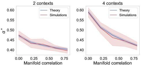
Figure S1: Capacity as a function of the manifold correlation, that for visibility purposes we take uniform $\Sigma^{\mu i}_{\nu j}=\sigma$ for all pairs of manifolds $(\mu,\nu)$ and directions $(i,j)$ with uncorrelated context hyperplanes for synthetic spherical manifolds of latent dimension $D=10$, embedded in ambient dimension $N=8000$. Left and right panels depict the capacity for $2$ and $4$ contexts respectively. Theory is depicted in blue while simulations in red. The full lines mark the average values and shaded bands represent one standard deviation.

References

Chung and Abbott (2021)S. Chung and L. Abbott, Curr. opin.
neurobiol. 70, 137
(2021).
Sorscher et al. (2022)B. Sorscher, S. Ganguli, and H. Sompolinsky, Proceedings of the
National Academy of Sciences 119, e2200800119 (2022).
Bernardi et al. (2020)S. Bernardi, M. K. Benna,
M. Rigotti, J. Munuera, S. Fusi, and C. D. Salzman, Cell 183, 954 (2020).
Ansuini et al. (2019)A. Ansuini, A. Laio,
J. H. Macke, and D. Zoccolan, Advances in Neural Information
Processing Systems 32 (2019).
Chung et al. (2018)S. Chung, D. D. Lee, and H. Sompolinsky, Physical Review
X 8, 031003 (2018).
Wakhloo et al. (2023)A. J. Wakhloo, T. J. Sussman, and S. Chung, Physical Review Letters 131, 027301 (2023).
Cohen et al. (2020)U. Cohen, S. Chung,
D. D. Lee, and H. Sompolinsky, Nature
communications (2020).
Kuoch et al. (2024)M. Kuoch, C.-N. Chou,
N. Parthasarathy, J. Dapello, J. J. DiCarlo, H. Sompolinsky, and S. Chung, in Conference on Parsimony and Learning (PMLR, 2024) pp. 395–418.
Froudarakis et al. (2020)E. Froudarakis, U. Cohen,
M. Diamantaki, E. Y. Walker, J. Reimer, P. Berens, H. Sompolinsky, and A. S. Tolias, BioRxiv (2020).
Yao et al. (2023)J. D. Yao, K. O. Zemlianova,
D. L. Hocker, C. Savin, C. M. Constantinople, S. Chung, and D. H. Sanes, Proceedings of the National Academy of
Sciences 120, e2212120120 (2023).
Paraouty et al. (2023)N. Paraouty, J. D. Yao,
L. Varnet, C.-N. Chou, S. Chung, and D. H. Sanes, Nature communications 14, 5828 (2023).
Chou et al. (2024)C.-N. Chou, L. Arend,
A. J. Wakhloo, R. Kim, W. Slatton, and S. Chung, BioArxiv (2024).
Mante et al. (2013)V. Mante, D. Sussillo,
K. V. Shenoy, and W. T. Newsome, nature 503, 78 (2013).
Buschman and Kastner (2015)T. J. Buschman and S. Kastner, Neuron 88, 127
(2015).
Panichello and Buschman (2021)M. F. Panichello and T. J. Buschman, Nature 592, 601
(2021).
Flesch et al. (2022)T. Flesch, K. Juechems,
T. Dumbalska, A. Saxe, and C. Summerfield, Neuron 110, 1258 (2022).
Moore and Armstrong (2003)T. Moore and K. M. Armstrong, Nature 421, 370
(2003).
Buschman and Miller (2007)T. J. Buschman and E. K. Miller, science 315, 1860
(2007).
Cukur et al. (2013)T. Cukur, S. Nishimoto,
A. G. Huth, and J. L. Gallant, Nature
neuroscience 16, 763
(2013).
Tavoni et al. (2021)G. Tavoni, D. E. C. Kersen, and V. Balasubramanian, PLoS computational biology 17, e1009479 (2021).
London and Häusser (2005)M. London and M. Häusser, Annu. Rev. Neurosci. 28, 503 (2005).
Budden et al. (2020)D. Budden, A. Marblestone,
E. Sezener, T. Lattimore, G. Wayne, and J. Veness, Advances in Neural Information Processing
Systems 33, 16508
(2020).
Veness et al. (2021)J. Veness et al., in Proceedings of the AAAI Conference on Artificial Intelligence, Vol. 35 (2021).
Saxe et al. (2022)A. Saxe, S. Sodhani, and S. J. Lewallen, in International Conference on
Machine Learning (PMLR, 2022) pp. 19287–19309.
Li and Sompolinsky (2022)Q. Li and H. Sompolinsky, Advances in Neural Information Processing Systems 35, 34789 (2022).
Gardner (1988)E. Gardner, Journal of physics A: Mathematical and general 21, 257 (1988).
Mézard et al. (1987)M. Mézard, G. Parisi,
and M. A. Virasoro, Spin glass theory and beyond: An
Introduction to the Replica Method and Its Applications, Vol. 9 (World Scientific Publishing Company, 1987).
Monasson and Zecchina (1995)R. Monasson and R. Zecchina, Modern Physics Letters B 9, 1887 (1995).
Baldassi et al. (2019)C. Baldassi, E. M. Malatesta, and R. Zecchina, Physical review letters 123, 170602 (2019).
Zavatone-Veth and Pehlevan (2021)J. A. Zavatone-Veth and C. Pehlevan, Physical Review E 103, L020301 (2021).
Cover (1965)T. M. Cover, IEEE
transactions on electronic computers (1965).
Nogueira et al. (2023)R. Nogueira, C. C. Rodgers, R. M. Bruno,
and S. Fusi, Nature
Neuroscience 26, 239
(2023).
David et al. (2004)S. V. David, W. E. Vinje, and J. L. Gallant, Journal of
Neuroscience 24, 6991
(2004).
Doi et al. (2012)E. Doi, J. L. Gauthier,
G. D. Field, J. Shlens, A. Sher, M. Greschner, T. A. Machado, L. H. Jepson, K. Mathieson, D. E. Gunning, et al., Journal of Neuroscience 32, 16256 (2012).
He et al. (2016)K. He, X. Zhang, S. Ren, and J. Sun, in Proceedings of the IEEE conference on computer vision and
pattern recognition (2016) pp. 770–778.
Stephenson et al. (2021)C. Stephenson et al., in ICLR 2021 (2021).
Musslick et al. (2017)S. Musslick, A. Saxe,
K. Özcimder, B. Dey, G. Henselman, and J. D. Cohen (Cognitive Science Society, 2017).
Aubin et al. (2018)B. Aubin, A. Maillard,
F. Krzakala, N. Macris, L. Zdeborová, et al., Advances in Neural
Information Processing Systems 31 (2018).
Loureiro et al. (2021)B. Loureiro, G. Sicuro,
C. Gerbelot, A. Pacco, F. Krzakala, and L. Zdeborová, Advances in Neural Information Processing
Systems 34, 10144
(2021).
Cornacchia et al. (2023)E. Cornacchia, F. Mignacco, R. Veiga,
C. Gerbelot, B. Loureiro, and L. Zdeborová, Machine Learning: Science and
Technology 4, 015019
(2023).