Peer influence on effort devoted to some activity is often studied using proxy variables when actual effort is unobserved. For instance, in education, academic effort is often proxied by GPA. We propose an alternative approach that circumvents this approximation. Our framework distinguishes unobserved shocks to GPA that do not affect effort from preference shocks that do affect effort levels. We show that peer effects estimates obtained using our approach can differ significantly from classical estimates (where effort is approximated) if the network includes isolated students. Applying our approach to data on high school students in the United States, we find that peer effect estimates relying on GPA as a proxy for effort are 40% lower than those obtained using our approach.

Keywords: Social networks, Peer effects, Academic achievement, Unobserved effort, Isolated agents

JEL classification: C31, J24

1   Introduction

In recent years, there has been a growing interest in the impact of peers on educational outcomes (Sacerdote, 2011; Epple and Romano, 2011). As peer effects on students’ academic effort may involve a social multiplier effect, understanding whether students are influenced by their friends and the size of this influence is crucial for evaluating policies aimed at improving academic achievement (Manski, 1993). However, estimating peer effects based on academic effort presents challenges, since effort is generally unobserved. Consequently, many empirical studies resort to using grade point average (GPA) as a proxy variable for effort. While microfounded models exploring the impact of peer interactions on academic achievement are often focused on effort (e.g., see Calvó-Armengol et al., 2009; Arcidiacono et al., 2012; Fruehwirth, 2013, 2014; Hong and Lee, 2017), GPA is typically employed in the empirical analysis because measures of student effort are unavailable. Yet, this approximation overlooks that GPA is not solely influenced by effort but also by many other factors, including unobserved student and school characteristics.

In this paper, we investigate the implications of using GPA as a proxy for academic effort on the estimation and interpretation of peer effects. We develop a structural model of educational effort with social interactions, in which students decide on their academic effort while taking into account that of their peers (friends), assuming complementarity between students’ and peers’ efforts. We also explicitly model the production function of academic achievement (GPA), which includes effort as a key input. Without using a proxy for student academic effort, we show that the model allows for identifying peer effects on academic effort. Furthermore, we demonstrate that the size of the effect may differ from that estimated using GPA as a proxy for effort, because the proxy-based approach suffers from an issue akin to an omitted variables problem. We derive a reduced-form equation for GPA, which differs from the classical linear-in-means peer effects specification, that highlights the need to control for two types of unobserved GPA shocks to disentangle peer effects on academic effort from other common effects captured by GPA. First, one needs to account for common shocks that directly influence GPA, such as improvements in teaching quality, irrespective of the effort level. These shocks result in a GPA increase for the same level of effort and do not involve a social multiplier effect. Second, one needs to account for common shocks affecting students’ preferences, such as increasing motivation to value academic achievement through information, which influence both academic effort and GPA, and may have social multiplier effects among students with friends.

We demonstrate that approximating student effort with GPA may result in biased estimates of peer effects when some students in the network do not have friends. This is because students who have friends are affected differently by the two types of GPA shocks mentioned above compared to those without friends. Standard approaches using GPA as a proxy fail to differentiate between these two types of shocks, leading to biased estimates of peer effects when the network includes students without friends. However, we show that in networks without isolated students, the standard model does not produce biased estimates of peer effects. The key difference between the reduced-form of the standard model and our framework is that while the standard model has a single intercept for each school, our approach accounts for unobserved school-level heterogeneity based on whether a student has friends or not. This amounts to introducing two types of fixed effects per school, one for students with friends and one for isolated students.

We illustrate the importance of this distinction through both a Monte Carlo simulation study and an empirical application using the National Longitudinal Study of Adolescent to Adult Health (Add Health) data. Estimating peer effects through our proposed method suggests that increasing the average GPA of peers by one point leads to a 0.856 point increase in students’ GPA. In contrast, the standard linear-in-means model using GPA as a proxy for student academic effort estimates this effect at 0.507. This substantial difference highlights that failing to account for two types of shocks at the school level may yield substantially biased estimates. The intuition behind this bias is that the standard approach misidentifies direct shocks to GPA that do not influence effort as effort shocks, thereby overestimating their impact through a social multiplier effect. Importantly, we also find that other plausible approaches, such as estimating a model that accounts for only one type of school-level shock and incorporating a dummy variable for isolated students, fail to rectify the bias, as does excluding isolated students from the sample.

Our econometric model incorporates two types of school-level unobserved shocks to GPA, which renders the well-known reflection problem more complex. In the case of the standard linear-in-means model, Bramoullé et al. (2009) provide straightforward conditions relating to the network structure under which the reflection problem is resolved. We extend their identification analysis to our framework; our main condition for identification requires that the network must include at least two students separated by a path of distance three, which is slightly stronger than the condition in Bramoullé et al. (2009).

We also extend our analysis to the case of endogenous networks. Network endogeneity can occur because we do not observe certain student characteristics, such as intellectual quotient (IQ), that may influence both students’ likelihood to form links with others and their GPA. We control for these unobserved characteristics using a two-stage estimation approach. Our method is nonparametric as in Johnsson and Moon (2021). We do not impose a specific parametric restriction in the relationship between the unobserved characteristics and GPA. Our approach is similar to generalized additive models (GAM), which are widely employed in the nonparametric regression literature (see Hastie, 2017).

Our structural model and econometric approach can also be applied to study peer influence on other outcomes that depend on exerted effort. An example is the body mass index (BMI), which cannot be directly chosen (e.g., Fortin and Yazbeck, 2015). People need to exert effort, such as developing healthy diet habits or engaging in physical exercise to improve their BMI. Peer influences are more related to effort than BMI. Another example is peer effects on a worker’s effort (e.g., Mas and Moretti, 2009; Cornelissen et al., 2017). The observed outcome is generally worker’s productivity, whereas peer effects take source in effort.

Related Literature

There is a large literature studying social interactions both theoretically and empirically (Durlauf and Ioannides, 2010; Blume et al., 2011). We follow the games in networks approach to the analysis of social interactions (see Jackson and Zenou, 2015, for a comprehensive overview of this literature). Ballester et al. (2006) analyze a noncooperative game with linear-quadratic utilities and strategic complementarities, in which each player decides how much effort they exert. Applying a similar framework to an education application, Calvó-Armengol et al. (2009) use GPA as a proxy for the exerted effort. We contribute to this strand of the literature by explicitly modelling the production function that captures how effort, along with other factors, translates into GPA, while distinguishing between unobserved shocks that directly impact GPA without affecting effort, from shocks that impact both academic effort and GPA. This leads to a reduced-form equation for GPA that differs from the standard linear-in-means peer effects specification.

This paper makes a methodological contribution to the extensive empirical literature on peer effects on educational outcomes (Sacerdote, 2011; Epple and Romano, 2011). We show both analytically and through an empirical application using AddHealth data that approximating student effort with GPA may result in biased estimates of peer effects, when some students in the network lack friends. Since isolated students are a common feature in many social network datasets, this finding highlights the limitations of using proxy variables, such as GPA, for estimating peer effects reliably.

Our paper also contributes to the econometric literature on peer effects (De Paula, 2017; Kline and Tamer, 2020) in two ways. First, a key challenge in this field is the reflection problem (Manski, 1993). A recent wave of papers have addressed this issue by imposing conditions on the network structure (Bramoullé et al., 2009; De Giorgi et al., 2010). Our contribution is to study the reflection problem in a setting where the GPA is influenced by various types of common shocks at the school level, and where students may have no peers. As in Bramoullé et al. (2009), our main identification condition involves the network structure and can be readily tested in empirical applications. Our second contribution lies in addressing the network endogeneity issue. We allow for unobserved attributes to influence students’ likelihood of forming links with others and their GPA (Goldsmith-Pinkham and Imbens, 2013; Hsieh and Lee, 2016; Johnsson and Moon, 2021). Unlike many studies that impose a strong parametric restriction between unobserved attributes and the peer effect model, we adopt a nonparametric approach to connect GPA to these attributes. Our approach is similar to the control function method used by Johnsson and Moon (2021), but it is adaptable to complex models. Specifically, we employ cubic B-splines, which are commonly used in Generalized Additive Models (GAM), to establish a smooth function linking the unobserved attributes and GPA (Hastie, 2017).

The remainder of the paper is organized as follows. Section 2 presents the microeconomic foundations of the model using a network game in which students decide their academic effort. Section 3 describes the econometric model and addresses the identification and estimation of the parameters. Section 4 presents our empirical analysis using Add Health data. Section 5 provides an extension of our framework to endogenous networks. Section 6 concludes this paper.

2   The Structural Model

In this section, we introduce a structural model based on a game of complete information, where students choose their effort level, which impacts their educational achievements (GPA). Students’ effort levels are also influenced by the effort exerted by their peers. This model can also be applied to investigating peer effects on other inputs that are not typically directly observed by the econometrician. For instance, it can be used to examine peer effects on (unobserved) effort in a workplace setting where observed productivity serves as the outcome. Another application is peer effects on effort directed toward improving BMI, such as adopting healthy diet habits or engaging in physical exercise, which is more readily observable than the effort itself.

We consider $S$ independent schools and denote by $n_{s}\geq 3$ the number of students in the $s$-th school, $s\in\{1,\dots,S\}$. Let $n$ be the total number of students, that is, $n=\sum_{s=1}^{S}n_{s}$. Each student $i$ in school $s$ has a GPA denoted by $y_{s,i}$ and observable characteristics represented by a $K$-vector $\mathbf{x}_{s,i}$. Students interact in their school through a directed network that can be represented by an $n_{s}\times n_{s}$ adjacency matrix $\mathbf{A}_{s}=[a_{s,ij}]_{ij}$, where $a_{s,ij}$ = 1 if student $j$ is $i^{\prime}s$ friend and $a_{s,ij}=0$ otherwise. We assume that $a_{s,ii}$ = 0 for all $i$ and $s$ so that students cannot interact with themselves. In addition, we only consider within-school interactions; students do not interact with peers in other schools (see Calvó-Armengol et al., 2009). We define the social interaction matrix $\mathbf{G}_{s}=[g_{s,ij}]_{ij}$ as the row-normalized adjacent matrix $\mathbf{A}_{s}$, that is, $g_{s,ij}=1/n_{s,i}$ if $j$ is a $i$’s friend and $g_{s,ij}=0$ otherwise, where $n_{s,i}$ is the number of friends of student $i$ within school $s$.

Student $i$ chooses their effort $e_{s,i}$, which in turn affects their GPA. More precisely, GPA is a function of student effort $e_{s,i}$, observable characteristics $\mathbf{x}_{s,i}$, and a random term $\eta_{s,i}$ that captures unobservable characteristics. Following Fruehwirth (2013) and Boucher and Fortin (2016), we posit that this relationship is given by the production function:

$$y_{s,i}=\alpha_{s}+\delta e_{s,i}+\mathbf{x}^{\prime}_{s,i}\boldsymbol{\theta}+\eta_{s,i},$$ (1)

where $\delta>0$ and $\alpha_{s}$ and $\boldsymbol{\theta}$ are unknown parameters. The parameter $\alpha_{s}$ captures unobserved school-level GPA shifters, such as teacher quality, operating as fixed effects. The linear production function is somewhat restrictive and can be generalized to a nonlinear or nonparametric production function (e.g., see Fruehwirth, 2013). However, identification of the resulting econometric model can be intractable, especially when the model allows for unobserved school heterogeneity.

The effort exerted and the GPA obtained provide students with a benefit that is captured by a payoff function, which, as in Calvó-Armengol et al. (2009) and Boucher and Fortin (2016), takes a linear-quadratic form:

$$u_{s,i}(e_{s,i},\mathbf{e}_{s,-i},y_{s,i})=\underbrace{(c_{s}+\mathbf{x}_{s,i}^{\prime}\boldsymbol{\beta}+\mathbf{g}_{s,i}\mathbf{X}_{s}\boldsymbol{\gamma}+\varepsilon_{s,i})y_{s,i}-\frac{e_{s,i}^{2}}{2}}_{\text{private sub-payoff}}+\underbrace{\lambda e_{s,i}\mathbf{g}_{s,i}\mathbf{e}_{s}}_{\text{social sub-payoff}},$$ (2)

where $\mathbf{X}_{s}=(\mathbf{x}_{s,1},\dots,\mathbf{x}_{s,n_{s}})^{\prime}$, $\mathbf{g}_{s,i}$ is the $i$-th row of $\mathbf{G}_{s}$, $\mathbf{e}_{s,-i}=(e_{s,1},\dots,e_{s,i-1},e_{s,i},\dots,e_{s,n})^{\prime}$, $\mathbf{e}_{s}=(e_{s,1},\dots,e_{s,n_{s}})^{\prime}$, the term $\mathbf{g}_{s,i}\mathbf{e}_{s}$ is the average effort of peers, and $c_{s}$, $\boldsymbol{\beta}$, $\boldsymbol{\gamma}$ are unknown parameters. The parameter $\lambda$ captures endogenous peer effects. The payoff function (2) encompasses two components: a private sub-payoff and a social sub-payoff. The term $(c_{s}+\mathbf{x}_{s,i}^{\prime}\boldsymbol{\beta}+\mathbf{g}_{s,i}\mathbf{X}_{s}\boldsymbol{\gamma}+\varepsilon_{s,i})$ represents the benefit enjoyed per unit of GPA achieved, where $\varepsilon_{s,i}$ is the student type (observable by all students). This benefit accounts for student observed heterogeneity, as it depends on $\mathbf{x}_{s,i}$ and peer group average characteristics $\mathbf{g}_{s,i}\mathbf{X}_{s}$ termed contextual variables (see Manski, 1993). The benefit also accounts for school unobserved heterogeneity through the parameter $c_{s}$. The second term of the private sub-payoff, $e_{s,i}^{2}/2$ reflects the cost of exerting effort. The social sub-payoff $\lambda e_{s,i}\mathbf{g}_{s,i}\mathbf{e}_{s}$ implies that an increase in the average peer group’s effort $\mathbf{g}_{s,i}\mathbf{e}_{s}$ influences student $i$’s marginal payoff if $\lambda\neq 0$. When $\lambda>0$, the payoff function (2) implies complementarity between students’ and peers’ efforts, whereas $\lambda<0$ indicates substitutability in efforts.

The parameters $\alpha_{s}$ and $c_{s}$ capture different unobserved shocks at the school level, and are conceptually different in terms of their policy implications. $\alpha_{s}$ captures unobserved shocks on GPA that do not affect student effort. These shocks, such as variation in teaching quality and school management, directly impact GPA irrespective of student effort. On the other hand, $c_{s}$ captures shocks on student preferences, particularly on the marginal payoff. For instance, interventions aimed at making students more aware of the returns to academic achievement could influence the marginal payoff. Such a shock can be captured by $c_{s}$ and would influence effort and consequently GPA through equation (1). We show that $\alpha_{s}$ and $c_{s}$ do not impact GPA in the same way (see Section 3.1).

By substituting $y_{s,i}$ from Equation (1) into Equation (2), we obtain a payoff function that does not depend on GPA (see Appendix A.1). This new payoff function defines a static game with complete information, in which students simultaneously choose their effort levels to maximize their payoff. The best response function for the students is given by:

$$e_{s,i}=\delta c_{s}+\lambda\mathbf{g}_{s,i}\mathbf{e}_{s}+\delta\mathbf{x}_{s,i}^{\prime}\boldsymbol{\beta}+\delta\mathbf{g}_{s,i}\mathbf{X}_{s}\boldsymbol{\gamma}+\delta\varepsilon_{s,i}.$$ (3)

In Equation (3), students’ levels of effort are expressed as a function of the average effort of their peers $\mathbf{g}_{s,i}\mathbf{e}_{s}$, observed students’ characteristics $\mathbf{x}_{s,i}$, and the average characteristics of peers $\mathbf{g}_{s,i}\mathbf{X}_{s}$ (contextual variables). The parameter $\lambda$ represents the impact of peers on a student’s effort level. A positive value of $\lambda$ indicates that a student’s effort level increases if their peers put in more effort. Furthermore, Equation (3) shows that the optimal effort level (and thus the resulting GPA) is influenced by shocks at the school level (on $c_{s}$) that affect student preferences. However, shocks directly affecting GPA through the parameter $\alpha_{s}$ do not impact effort.

The best response function (3) in matrix form can be expressed as $\mathbf{e}_{s}=\delta c_{s}\mathbf{1}_{n_{s}}+\lambda\mathbf{G}_{s}\mathbf{e}_{s}+\delta\mathbf{X}_{s}\boldsymbol{\beta}+\delta\mathbf{G}_{s}\mathbf{X}_{s}\boldsymbol{\gamma}+\delta\boldsymbol{\varepsilon}_{s}$, where $\boldsymbol{\varepsilon}_{s}=(\varepsilon_{s,1},\dots,\varepsilon_{s,n_{s}})^{\prime}$ and $\mathbf{1}_{n_{s}}$ is an $n_{s}$-vector of ones. A solution of this equation in $\mathbf{e}_{s}$ is a Nash equilibrium (NE) of the game. As $\mathbf{G}_{s}$ is row-normalized, the NE is unique under Assumption 2.1 and can be expressed as $\mathbf{e}_{s}=(\mathbf{I}_{n_{s}}-\lambda\mathbf{G}_{s})^{-1}(\delta c_{s}\mathbf{1}_{n_{s}}+\delta\mathbf{X}_{s}\boldsymbol{\beta}+\delta\mathbf{G}_{s}\mathbf{X}_{s}\boldsymbol{\gamma}+\delta\boldsymbol{\varepsilon}_{s})$, where $\mathbf{I}_{n_{s}}$ is the $n_{s}\times n_{s}$ identity matrix (see Appendix A.1).

Assumption 2.1.

$|\lambda|<1$.

The condition $|\lambda|<1$ implies that students do not increase (in absolute value) their effort as much as the increase in the effort of their peers. Put differently, when the average effort of a student’s friends increases by one unit, the corresponding change in the student’s own effort is less than one unit in absolute value.

3   The Econometric Model and Identification Strategy

If effort were directly observable, we could estimate the peer effect parameter from Equation (3) following Kelejian and Prucha (1998). However, as we do not observe effort, the equation cannot be estimated directly. Instead, we derive from this equation an estimable equation based on GPA, which is influenced by effort. We show that this equation is econometrically different from the equation that we obtain if we proxy effort using GPA in Equation (2). We also present an identification strategy to identify the peer effect parameter $\lambda$ in the effort equation.

3.1 Reduced-Form Equation for GPA

From Equation (1), we express effort as a function of GPA and replace this expression in Equation (3). This yields a reduced-form equation for GPA that does not directly depend on effort (see Appendix A.2). The equation is given by

$$y_{s,i}=\kappa_{s,i}+\lambda\mathbf{g}_{s,i}\mathbf{y}_{s}+\mathbf{x}^{\prime}_{s,i}\boldsymbol{\tilde{\beta}}+\mathbf{g}_{s,i}\mathbf{X}_{s}\boldsymbol{\tilde{\gamma}}+(\boldsymbol{\omega}_{s,i}-\lambda\mathbf{g}_{s,i})\boldsymbol{\eta}_{s}+\delta^{2}\varepsilon_{s,i},$$ (4)

where $\kappa_{s,i}=\delta^{2}c_{s}+(1-\lambda\mathbf{g}_{s,i}\mathbf{1}_{n_{s}})\alpha_{s}$, $\boldsymbol{\tilde{\beta}}=\delta^{2}\boldsymbol{\beta}+\boldsymbol{\theta}$, $\boldsymbol{\tilde{\gamma}}=\delta^{2}\boldsymbol{\gamma}-\lambda\boldsymbol{\theta}$, and $\boldsymbol{\omega}_{s,i}$ is a row-vector of dimension $n_{s}$ in which all the elements are zero, except the $i$-th element, which is one.

If instead, we proxy effort by GPA in the payoff function (2), the resulting reduced-form equation of GPA would be:

$$y_{s,i}=\bar{c}_{s}+\bar{\lambda}\mathbf{g}_{s,i}\mathbf{y}_{s}+\mathbf{x}_{s,i}^{\prime}\boldsymbol{\bar{\beta}}+\delta\mathbf{g}_{s,i}\mathbf{X}_{s}\boldsymbol{\bar{\gamma}}+\bar{\varepsilon}_{s,i},$$ (5)

where $\bar{\lambda}$ is the peer effect parameter, $\boldsymbol{\bar{\beta}}$ and $\boldsymbol{\bar{\gamma}}$ measure the effects of own and contextual characteristics, $\bar{c}_{s}$ controls for unobserved school heterogeneity and $\bar{\varepsilon}_{s,i}$ is an error term. We will refer to this specification as the standard (classical) model.

Let $\mathcal{V}^{NI}_{s}$ denote the subsample of students of school $s$ who have friends (non-isolated) and $\mathcal{V}^{I}_{s}$ denote the subsample of students of school $s$ who have no friends (isolated). As $\mathbf{G}_{s}$ is row-normalized, we have $\mathbf{g}_{s,i}\mathbf{1}_{n_{s}}=1$ if $i\in\mathcal{V}^{NI}_{s}$ and $\mathbf{g}_{s,i}\mathbf{1}_{n_{s}}=0$ otherwise. Thus, $\kappa_{s,i}=\kappa^{I}_{s}$ if $i\in\mathcal{V}^{I}_{s}$ and $\kappa_{s,i}=\kappa^{NI}_{s}$ if $i\in\mathcal{V}^{NI}_{s}$, where $\kappa^{I}_{s}=\delta^{2}c_{s}+\alpha_{s}$ and $\kappa^{NI}_{s}=\delta^{2}c_{s}+(1-\lambda)\alpha_{s}$. If there are no isolated students in the network, $\kappa_{s,i}$ would be a simple school fixed effect, and our framework would be equivalent to the classical model. The difference between the standard model and our framework is that the standard model has a single intercept term per school. In Equation (4), $\kappa_{s,i}$ accounts for unobserved school-level heterogeneity depending on whether the student $i$ has friends or not. We would have $\kappa^{NI}_{s}=\kappa^{I}_{s}$ if and only if $\alpha_{s}=0$, $\lambda=0$, or if every student has friends. These conditions may not hold in many settings.

To appropriately account for the unobserved factor $\kappa_{s,i}$ in Equation (4), the above discussion suggests that we need to incorporate both school-fixed effects and a school-specific variable indicating whether a student has friends or not. This involves including $S$ school dummy variables and $S$ dummy variables indicating whether each student has friends or not. Each of the latter dummy variables corresponds to one school and takes the value of one if the student has friends. The rationale for this lies in the distinction between $\alpha_{s}$ and $c_{s}$, which affect GPA differently. To understand why distinguishing between these two shocks requires controlling for whether a student is isolated or not, it is important to consider the implications of the two shocks. As per Equations (3) and (4), an increase in $\alpha_{s}$ (e.g., by improving teaching quality) suggests an increase in GPA without affecting effort. Importantly, this increase does not depend on whether the student is isolated and does not involve a social multiplier effect. In contrast, a preference shock on $c_{s}$ could result in a social multiplier effect on the effort (according to Equation (3)), and thereby on GPA. This social multiplier effect is only present among students who have friends. Therefore, the distinction between the two types of shocks is essentially captured by the student’s social status: unlike for $\alpha_{s}$, the impact of $c_{s}$ on GPA is contingent upon whether the student is isolated or not.

The main distinction between the standard model and Equation (4) arises due to an omitted variables problem inherent in the standard model. These omitted variables are $-\lambda\alpha_{s}\mathbf{g}_{s,i}\mathbf{1}_{n_{s}}$, for $s=1,\dots,S$, and may introduce a significant discrepancy between the peer effect estimates of the two models. Following the logic of omitted variable bias (Theil, 1957), we know that the difference between the peer effect estimate from the standard model and the estimate from our specification has the same sign as the partial correlation between $-\lambda\alpha_{s}\mathbf{g}_{s,i}\mathbf{1}_{n_{s}}$ and $\mathbf{g}_{s,i}\mathbf{y}_{s}$. In most scenarios, it will be the sign of $-\lambda\alpha_{s}$ if $\mathbf{y}_{s}$ is nonnegative. This suggests that peer effects estimated using the standard model would be underestimated compared to the estimate from our specification if $\lambda\alpha_{s}>0$.

3.2 Identification and Estimation

As the effort $e_{s,i}$ is not observed, not all the parameters of the structural model can be identified. Specifically, $\delta$ cannot be identified because it only appears in Equation (4) through a product with other parameters. Similarly, $\boldsymbol{\theta}$ and $\boldsymbol{\gamma}$ cannot be identified separately, as they only appear in the expression of $\boldsymbol{\tilde{\gamma}}$. Nevertheless, we can identify the composite parameters $\boldsymbol{\tilde{\beta}}=\delta^{2}\boldsymbol{\beta}+\boldsymbol{\theta}$ and $\boldsymbol{\tilde{\gamma}}=\delta^{2}\boldsymbol{\gamma}-\lambda\boldsymbol{\theta}$, which are parameters in the reduced-form equation (4) that capture the causal effects of students’ characteristics $\mathbf{x}$ and average friends’ characteristics $\bar{\mathbf{x}}$ on GPA. Consequently, it is not necessary to identify $\delta$ and $\boldsymbol{\theta}$ to estimate these causal effects.

Let $n^{NI}_{s}$ denote the number of students in school $s$ with peers, and $n^{I}_{s}$ the number of students in the school $s$ without peers. Let also $\boldsymbol{\ell}^{NI}_{s}=\mathbf{G}_{s}\mathbf{1}_{n_{s}}$ and $\boldsymbol{\ell}^{I}_{s}=\mathbf{1}_{n_{s}}-\boldsymbol{\ell}^{NI}_{s}$. Equation (4) can be written in matrix form at the school level as

$$\mathbf{y}_{s}=\kappa^{I}_{s}\boldsymbol{\ell}^{I}_{s}+\kappa^{NI}_{s}\boldsymbol{\ell}^{NI}_{s}+\lambda\mathbf{G}_{s}\mathbf{y}_{s}+\mathbf{X}_{s}\boldsymbol{\tilde{\beta}}+\mathbf{G}_{s}\mathbf{X}_{s}\boldsymbol{\tilde{\gamma}}+(\mathbf{I}_{n_{s}}-\lambda\mathbf{G}_{s})\boldsymbol{\eta}_{s}+\delta^{2}\boldsymbol{\varepsilon}_{s}.$$ (6)

Note that the number of unknown parameters to be estimated in Equation (6) grows to infinity with the number of schools (there are $2S$ dummy variables). This issue is known as an incidental parameter problem and may lead to inconsistent estimators (Lancaster, 2000). A common approach to consistently estimate the model is to eliminate the fixed effects $\kappa^{I}_{s}$ and $\kappa^{NI}_{s}$. To do so, we define $\mathbf{J}_{s}:=\mathbf{I}_{n_{s}}-\dfrac{1}{n^{I}_{s}}\boldsymbol{\ell}^{I}_{s}\boldsymbol{\ell}^{I\prime}_{s}-\dfrac{1}{n^{NI}_{s}}\boldsymbol{\ell}^{NI}_{s}\boldsymbol{\ell}^{NI\prime}_{s}$ and impose by convention that $\dfrac{1}{n^{I}_{s}}\boldsymbol{\ell}^{I}_{s}\boldsymbol{\ell}^{I\prime}_{s}=0$ if $n^{I}_{s}=0$, and that $\dfrac{1}{n^{NI}_{s}}\boldsymbol{\ell}^{NI}_{s}\boldsymbol{\ell}^{NI\prime}_{s}=0$ if $n^{NI}_{s}=0$. Note that $\boldsymbol{\ell}^{NI\prime}_{s}\boldsymbol{\ell}^{NI}_{s}=\hat{n}_{s}$, $\boldsymbol{\ell}^{I\prime}_{s}\boldsymbol{\ell}^{I}_{s}=n^{I}_{s}$, $\boldsymbol{\ell}^{NI\prime}_{s}\boldsymbol{\ell}^{I}_{s}=0$, $\boldsymbol{\ell}^{I\prime}_{s}\boldsymbol{\ell}^{NI}_{s}=0$. Thus, $\mathbf{J}_{s}\boldsymbol{\ell}^{I}_{s}=\mathbf{J}_{s}\boldsymbol{\ell}^{NI}_{s}=0$. One can eliminate the term $\kappa^{I}_{s}\boldsymbol{\ell}^{I}_{s}+\kappa^{NI}_{s}\boldsymbol{\ell}^{NI}_{s}$ by premultiplying each term of Equation (6) by the matrix $\mathbf{J}_{s}$. This implies that

$$\mathbf{J}_{s}\mathbf{y}_{s}=\lambda\mathbf{J}_{s}\mathbf{G}_{s}\mathbf{y}_{s}+\mathbf{J}_{s}\mathbf{X}_{s}\boldsymbol{\tilde{\beta}}+\mathbf{J}_{s}\mathbf{G}_{s}\mathbf{X}_{s}\boldsymbol{\tilde{\gamma}}+\mathbf{J}_{s}(\mathbf{I}_{n_{s}}-\lambda\mathbf{G}_{s})\boldsymbol{\eta}_{s}+\delta^{2}\mathbf{J}_{s}\boldsymbol{\varepsilon}_{s}.$$ (7)

The random term $\boldsymbol{v}_{s}:=\mathbf{J}_{s}(\mathbf{I}_{n_{s}}-\lambda\mathbf{G}_{s})\boldsymbol{\eta}_{s}+\delta^{2}\mathbf{J}_{s}\boldsymbol{\varepsilon}_{s}$ is comprised of two error vectors $\boldsymbol{\eta}_{s}$ and $\boldsymbol{\varepsilon}_{s}$. To consistently estimate $\boldsymbol{\psi}:=(\lambda,\leavevmode\nobreak\ \boldsymbol{\tilde{\beta}}^{\prime},\leavevmode\nobreak\ \boldsymbol{\tilde{\gamma}}^{\prime})^{\prime}$, we impose the following assumption.

Assumption 3.1.

For any $s=1,\dots,S$, $\mathbb{E}(\boldsymbol{\eta}_{s}|\mathbf{G}_{s},\mathbf{X}_{s})=0$ and $\mathbb{E}(\boldsymbol{\varepsilon}_{s}|\mathbf{G}_{s},\mathbf{X}_{s})=0$

Assumption 3.1 implies that $\mathbf{X}_{s}$ and $\mathbf{G}_{s}$ are exogenous with respect to $\boldsymbol{\eta}_{s}$ and $\boldsymbol{\varepsilon}_{s}$. This suggests that there is no omission of important variables in $\mathbf{X}_{s}$, which are captured by $\boldsymbol{\eta}_{s}$ and $\boldsymbol{\varepsilon}_{s}$. We later relax this assumption in our approach to controlling for network endogeneity by allowing for $\mathbf{X}_{s}$ and $\mathbf{G}_{s}$ to depend on $\boldsymbol{\eta}_{s}$ and $\boldsymbol{\varepsilon}_{s}$ through unobserved factors to the econometrician (see Section 5).

Identification and Estimation of $\boldsymbol{\psi}$

Identification in peer effects models can be challenging, particularly due to the reflection problem (Manski, 1993). Bramoullé et al. (2009) address this problem and provide necessary and sufficient conditions for identification. Their main condition requires that $\mathbf{I}_{n_{s}}$, $\mathbf{G}_{s}$, $\mathbf{G}_{s}^{2}$, and $\mathbf{G}_{s}^{3}$ are linearly independent. However, their approach does not apply to our framework because their identification results assume that there are no isolated students (see their main assumption in their Section 2.1).

Given that existing identification results do not directly apply to our model, we extend the analysis in Bramoullé et al. (2009). We derive easy-to-verify conditions to address the reflection problem when the network includes students without friends.

Assumption 3.2.

(i) $\lambda\boldsymbol{\tilde{\beta}}+\boldsymbol{\tilde{\gamma}}\neq 0$; (ii) There are students in the network separated by a link of distance three.

Condition (i) is equivalent to stating that GPA is influenced by at least one contextual variable. With several characteristics in $\mathbf{X}_{s}$, this condition can be satisfied. Condition (ii) is slightly stronger than the assumption that $\mathbf{I}_{n_{s}}$, $\mathbf{G}_{s}$, $\mathbf{G}_{s}^{2}$, and $\mathbf{G}_{s}^{3}$ are linearly independent. It means that there are students who have connections to students that extend to three degrees of separation—friends of friends of friends—who are neither directly their friends nor friends of their friends (see an illustration in Figure 1 below). As we allow isolated students, Assumption 3.2 is not a necessary condition for identification, as is the case in Bramoullé et al. (2009); rather, it is a sufficient condition that holds in many cases.

Under Assumption 3.2, we show that $\boldsymbol{\psi}$ is identified. We estimate $\boldsymbol{\psi}$ using a standard GMM approach. It is well known that the regressor $\mathbf{J}_{s}\mathbf{G}_{s}\mathbf{y}_{s}$ is endogenous in Equation (7). However, it can be instrumented by $\mathbf{J}_{s}\mathbf{G}_{s}^{2}\mathbf{X}_{s}$, as suggested by Kelejian and Prucha (1998) and Bramoullé et al. (2009). Let $\boldsymbol{\hat{\psi}}$ be the GMM estimator of $\boldsymbol{\psi}$. We have the following result.

Proposition 3.1.

Under Assumptions 2.1–3.2 and A.1 (stated in Appendix A.3), $\boldsymbol{\psi}$ is globally identified, $\boldsymbol{\hat{\psi}}$ is a consistent estimator, and $\displaystyle\sqrt{n}(\boldsymbol{\hat{\psi}}-\boldsymbol{\psi}_{0})\overset{d}{\to}\mathcal{N}\big{(}0,\lim_{n\to\infty}n\operatorname{\mathbb{V}}(\boldsymbol{\hat{\psi}})\big{)}$, where $\boldsymbol{\psi}_{0}$ is the true value of $\boldsymbol{\psi}$.

The consistency and asymptotic normality of $\boldsymbol{\hat{\psi}}$ are directly derived from Kelejian and Prucha (1998). We later discuss how the asymptotic variance of $\boldsymbol{\hat{\psi}}$ can be estimated.

We show that the reflection problem arises within a network with links of distance three only when variations in friends’ average characteristics have no influence on students’ outcomes, which would directly contradict Condition (i) of Assumption 3.2. Below, we provide an intuition behind our identification approach and a formal proof in Appendix A.3. Figure 1 presents an example of a network with a link of distance three: $i_{2}$ is at three nodes from $i_{1}$; they are a friend of a friend of a friend of $i_{1}$. The reflection problem arises when $\mathbb{E}(\mathbf{J}_{s}\mathbf{G}_{s}\mathbf{y}_{s}|\mathbf{G}_{s},\mathbf{X}_{s})$ is perfectly collinear with $\mathbf{J}_{s}\mathbf{X}_{s}$ and $\mathbf{J}_{s}\mathbf{G}_{s}\mathbf{X}_{s}$. For a non-isolated student, this collinearity is equivalent to saying that there exist vector of parameters, $\dot{\boldsymbol{\beta}}$ and $\dot{\boldsymbol{\gamma}}$, such that $\mathbb{E}(\mathbf{g}_{s,i}\mathbf{y}_{s}-y^{NI}_{s}|\mathbf{G}_{s},\mathbf{X}_{s})=(\mathbf{x}_{s,i}-\mathbf{\hat{x}}_{s})^{\prime}\dot{\boldsymbol{\beta}}+(\mathbf{g}_{s,i}\mathbf{X}_{s}-\bar{\mathbf{x}}^{NI}_{s})^{\prime}\dot{\boldsymbol{\gamma}}$, where $y^{NI}_{s}$, $\mathbf{x}^{NI}_{s}$, and $\bar{\mathbf{x}}^{NI}_{s}$ are respectively the averages of $\mathbf{g}_{s,i}\mathbf{y}_{s}$, $\mathbf{x}_{s,i}$, and $\mathbf{g}_{s,i}\mathbf{X}_{s}$ in $\mathcal{V}^{NI}_{s}$. The variables $\mathbf{g}_{s,i}\mathbf{y}_{s}$, $\mathbf{x}_{s,i}$, and $\mathbf{g}_{s,i}\mathbf{X}_{s}$ are taken in deviation with respect to their average in $\mathcal{V}^{NI}_{s}$ because of the matrix $\mathbf{J}_{s}$ that multiplies the terms of Equation (7). If we take the previous equation in difference between students $i_{1}$ and $i_{3}$, we obtain

$$\mathbb{E}(\mathbf{g}_{s,i_{1}}\mathbf{y}_{s}-\mathbf{g}_{s,i_{3}}\mathbf{y}_{s}|\mathbf{G}_{s},\mathbf{X}_{s})=(\mathbf{x}_{s,i_{1}}-\mathbf{x}_{s,i_{3}})^{\prime}\dot{\boldsymbol{\beta}}+(\mathbf{g}_{s,i_{1}}\mathbf{X}_{s}-\mathbf{g}_{s,i_{3}}\mathbf{X}_{s})^{\prime}\dot{\boldsymbol{\gamma}}.$$ (8)

As $i_{3}$ is $i_{1}$’s only friend and $i_{4}$ is $i_{3}$’s only friend, we have $\mathbf{g}_{s,i_{1}}\mathbf{y}_{s}=y_{s,i_{3}}$, $\mathbf{g}_{s,i_{3}}\mathbf{y}_{s}=y_{s,i_{4}}$, $\mathbf{g}_{s,i_{1}}\mathbf{X}_{s}=\mathbf{x}_{s,i_{3}}$, and $\mathbf{g}_{s,i_{3}}\mathbf{X}_{s}=\mathbf{x}_{s,i_{4}}$. Thus Equation (8) implies $y_{i_{3}}^{e}-y_{i_{4}}^{e}=(\mathbf{x}_{s,i_{1}}-\mathbf{x}_{s,i_{3}})^{\prime}\dot{\boldsymbol{\beta}}+(\mathbf{x}_{s,i_{3}}-\mathbf{x}_{s,i_{4}})^{\prime}\dot{\boldsymbol{\gamma}}$, where $y_{i}^{e}=\mathbb{E}(y_{s,i}|\mathbf{G}_{s},\mathbf{X}_{s})$. As $\mathbf{x}_{s,i_{2}}$ does not appear in the previous equation, we can say that $y_{i_{3}}^{e}-y_{i_{4}}^{e}$ is independent of $\mathbf{x}_{s,i_{2}}$, conditional on $\mathbf{x}_{s,i_{1}}$, $\mathbf{x}_{s,i_{3}}$ and $\mathbf{x}_{s,i_{4}}$. Put differently, an increase in $\mathbf{x}_{s,i_{2}}$(ceteris paribus) has no impact on $y_{i_{3}}^{e}-y_{i_{4}}^{e}$, which means that the increase has either no impact on $y_{i_{3}}^{e}$ and $y_{i_{4}}^{e}$ or the same impact on $y_{i_{3}}^{e}$ and $y_{i_{4}}^{e}$. The first implication is not possible because $\mathbf{x}_{s,i_{2}}$ is the vector of contextual variables for $i_{4}$ and Condition (i) of Assumption 3.2 implies that GPA is influenced by at least one contextual variable. Moreover, $\mathbf{x}_{s,i_{2}}$ cannot influence $y_{i_{3}}^{e}$ and $y_{i_{4}}^{e}$ in the same way because $i_{2}$ is a direct friend of $i_{4}$ and not directly linked to $i_{3}$. This is in contradiction to equation (8), therefore, $\mathbb{E}(\mathbf{J}_{s}\mathbf{G}_{s}\mathbf{y}_{s}|\mathbf{G}_{s},\mathbf{X}_{s})$ cannot be a linear combination of $\mathbf{J}_{s}\mathbf{X}_{s}$ and $\mathbf{J}_{s}\mathbf{G}_{s}\mathbf{X}_{s}$.

Figure 1: Solving the reflection problem

Note: $\rightarrow$ means that the node on the right side is a friend of the node on the left side.

Asymptotic variance of $\boldsymbol{\hat{\psi}}$

We now discuss how the asymptotic variance of $\boldsymbol{\hat{\psi}}$ can be consistently estimated. One simple approach is to use the robust estimator à la White (1980) that allows for the variance of the component of $\boldsymbol{\eta}_{s}$ and $\boldsymbol{\varepsilon}_{s}$ to vary across schools. Let $\mathbf{\tilde{X}}_{s}=\mathbf{J}_{s}[\mathbf{X}_{s},\leavevmode\nobreak\ \mathbf{G}_{s}\mathbf{X}_{s}]$, $\mathbf{R}_{s}=[\mathbf{J}_{s}\mathbf{G}_{s}\mathbf{y}_{s},\leavevmode\nobreak\ \mathbf{\tilde{X}}_{s}]$, $\mathbf{Z}_{s}=[\mathbf{J}_{s}\mathbf{G}_{s}^{2}\mathbf{X}_{s},\leavevmode\nobreak\ \mathbf{\tilde{X}}_{s}]$, $\mathbf{R}^{\prime}\mathbf{Z}=\sum_{s=1}^{S}\mathbf{R}^{\prime}_{s}\mathbf{Z}_{s}$, $\mathbf{Z}^{\prime}\mathbf{Z}=\sum_{s=1}^{S}\mathbf{Z}^{\prime}_{s}\mathbf{Z}_{s}$. Let also $\hat{\boldsymbol{v}}_{s}:=\mathbf{J}_{s}\mathbf{y}_{s}-\mathbf{R}_{s}\boldsymbol{\hat{\psi}}$, that is, $\hat{\boldsymbol{v}}_{s}$ is the residual vector from Equation (7). We denote by $\operatorname{diag}$ the bloc diagonal matrix operator. The asymptotic variance of $\boldsymbol{\hat{\psi}}$ can be estimated by $\mathbf{\hat{B}}_{n}^{-1}\mathbf{\hat{D}}_{n}\mathbf{\hat{B}}_{n}^{-1}/n$, where $\mathbf{\hat{B}}_{n}=(\mathbf{R}^{\prime}\mathbf{Z})(\mathbf{Z}^{\prime}\mathbf{Z})^{-1}(\mathbf{R}^{\prime}\mathbf{Z})^{\prime}/n$ and $\mathbf{\hat{D}}_{n}=(\mathbf{R}^{\prime}\mathbf{Z})(\mathbf{Z}^{\prime}\mathbf{Z})^{-1}\operatorname{diag}\{\mathbf{Z}_{1}^{\prime}\hat{\boldsymbol{v}}_{1}\hat{\boldsymbol{v}}_{1}^{\prime}\mathbf{Z}_{1},\dots,\mathbf{Z}_{S}^{\prime}\hat{\boldsymbol{v}}_{S}\hat{\boldsymbol{v}}_{S}^{\prime}\mathbf{Z}_{S}\}(\mathbf{Z}^{\prime}\mathbf{Z})^{-1}(\mathbf{R}^{\prime}\mathbf{Z})^{\prime}/n$.

However, for this estimator of the asymptotic variance, we need to impose that $n_{s}$ is bounded, that is, the network is composed of many bounded and independent schools. This assumption is important for $\mathbf{Z}_{s}^{\prime}\hat{\boldsymbol{v}}_{s}$ to be $O_{p}(1)$ and have a second-order moment. We also present another estimator that does not require this condition. This estimator is based on the covariance structure of the error term $\boldsymbol{v}_{s}$. For this second approach, we set the following assumptions.

Assumption 3.3.

(i) $\mathbf{G}_{s}$is uniformly bounded in column sum; (ii) $\lambda\neq 0$; (iii) $(\eta_{s,i},\leavevmode\nobreak\ \varepsilon_{s,i})$is independently distributed across $i$ such that $\mathbb{E}(\eta_{s,i}^{2}|\mathbf{G}_{s},\mathbf{X}_{s})=\sigma_{\eta}^{2}>0$, $\mathbb{E}((\delta^{2}\varepsilon_{s,i})^{2}|\mathbf{G}_{s},\mathbf{X}_{s})=\sigma_{\epsilon}^{2}>0$, $\mathbb{E}(\delta^{2}\varepsilon_{s,i}\eta_{s,i}|\mathbf{G}_{s},\mathbf{X}_{s})=\rho\sigma_{\eta}\sigma_{\epsilon}$, and $\lvert\rho\rvert\leq 1$.

If both $S$ and $n_{s}$ tend to infinity, Condition (i) rules out the cases where the sum of certain columns of $\mathbf{G}_{s}$ is unbounded. This condition is also considered by (Lee, 2004) in the case of the standard model. Condition (iii) imposes constant variances for the error terms $\eta_{s,i}$ and $\varepsilon_{s,i}$ but accounts for their potential correlation. This is important as $\eta_{s,i}$ and $\varepsilon_{s,i}$ characterize the same student $i$. The parameter $\rho$ measures the correlation between $\eta_{s,i}$ and $\varepsilon_{s,i}$. We impose no restrictions on the joint distribution of $(\eta_{s,i},\leavevmode\nobreak\ \varepsilon_{s,i})$. The restriction $\lambda\neq 0$ of Condition (ii) is necessary for identifying $\sigma_{\eta}$, $\sigma_{\epsilon}$, and $\rho$. If $\lambda=0$, the disturbance of Equation (7) would be $\mathbf{J}_{s}\boldsymbol{\eta}_{s}+\delta^{2}\mathbf{J}_{s}\boldsymbol{\varepsilon}_{s}$, and one cannot disentangle $\sigma_{\eta}$, $\sigma_{\epsilon}$, and $\rho$.

Under Assumption 3.3, we can estimate $(\sigma_{\eta}^{2},\leavevmode\nobreak\ \sigma_{\epsilon}^{2},\leavevmode\nobreak\ \rho)$ and construct a consistent estimator for $\operatorname{\mathbb{V}}(\boldsymbol{\hat{\psi}})$. We employ a quasi-maximum likelihood (QML) approach, where the dependent variable is the vector of the residual vector $\hat{\boldsymbol{v}}_{s}=\mathbf{J}_{s}\mathbf{y}_{s}-\mathbf{R}_{s}\boldsymbol{\hat{\psi}}$. The likelihood of $\hat{\boldsymbol{v}}_{s}$ is based on a multivariate normal distribution with mean and covariance matrix equal to those of the true error term $\boldsymbol{v}_{s}$, where $\lambda$ is replaced by its estimator $\hat{\lambda}$. Importantly, we do not require $\boldsymbol{v}_{s}$ to be actually normally distributed. Let $(\hat{\sigma}_{\eta}^{2},\leavevmode\nobreak\ \hat{\sigma}_{\epsilon}^{2},\leavevmode\nobreak\ \hat{\rho})$ be the QML estimator of $(\sigma_{\varepsilon}^{2},\leavevmode\nobreak\ \sigma_{\epsilon}^{2},\leavevmode\nobreak\ \rho)$. We establish the following result.

Proposition 3.2.

Under Proposition 3.1 and Assumptions A.2–A.4 stated in Appendix A.4, $(\sigma_{\epsilon}^{2},\leavevmode\nobreak\ \sigma_{\epsilon}^{2},\leavevmode\nobreak\ \rho)$ is globally identified, and $(\hat{\sigma}_{\eta}^{2},\leavevmode\nobreak\ \hat{\sigma}_{\epsilon}^{2},\leavevmode\nobreak\ \hat{\rho})$ is a consistent estimator.

We can now consistently estimate the asymptotic variance of $\boldsymbol{\hat{\psi}}$ using the estimator $(\hat{\sigma}_{\eta}^{2},\leavevmode\nobreak\ \hat{\sigma}_{\epsilon}^{2},\leavevmode\nobreak\ \hat{\rho})$. We denote by $\mathbf{B}=\operatorname{plim}(\mathbf{R}^{\prime}\mathbf{Z})(\mathbf{Z}^{\prime}\mathbf{Z})^{-1}(\mathbf{R}^{\prime}\mathbf{Z})^{\prime}/n$, where $\operatorname{plim}$ stands for the limit in probability as $n$ grows to infinity. We also define $\boldsymbol{\check{\Omega}}=\sum_{s=1}^{S}\mathbf{Z}_{s}^{\prime}\big{(}\sigma_{\epsilon}^{2}\mathbf{J}_{s}+\sigma_{\eta}^{2}\mathbf{J}_{s}^{\prime}\mathbf{W}_{s}\mathbf{W}_{s}^{\prime}\mathbf{J}_{s}+\rho\sigma_{\epsilon}\sigma_{\eta}\mathbf{J}_{s}(\mathbf{W}_{s}+\mathbf{W}_{s}^{\prime})\mathbf{J}_{s})\big{)}\mathbf{Z}_{s}$. We make the assumption that $\operatorname{plim}(\mathbf{R}^{\prime}\mathbf{Z})(\mathbf{Z}^{\prime}\mathbf{Z})^{-1}\boldsymbol{\check{\Omega}}(\mathbf{Z}^{\prime}\mathbf{Z})^{-1}(\mathbf{R}^{\prime}\mathbf{Z})^{\prime}/n$ exists and is denoted by $\mathbf{D}$. As a result $\displaystyle\lim_{n\to\infty}n\operatorname{\mathbb{V}}(\boldsymbol{\hat{\psi}})=\mathbf{B}^{-1}\mathbf{D}\mathbf{B}^{-1}$. We can obtain a consistent estimator of the variance by replacing $\sigma_{\epsilon}^{2}$, $\sigma_{\eta}^{2}$, and $\rho$ with their estimator, and $\mathbf{B}$ and $\mathbf{D}$ with their empirical counterparts.

3.3 Simulation Study

In this section, we conduct a simulation study to illustrate the importance of controlling for separate school fixed effects for isolated and non-isolated students. We consider a scenario with $S=20$ schools, each school having $n_{s}=50$ students. The network is defined such that student $i$ in school $s$ has $n_{s,i}$ friends chosen randomly among their schoolmates. We randomly assign to $n_{s,i}$ a value in $\{0,\leavevmode\nobreak\ 1,\leavevmode\nobreak\ \dots,\leavevmode\nobreak\ 10\}$ according to the probability distribution given by $\mathbb{P}(n_{s,i}=k)=\dfrac{\pi}{(1+k)^{0.6}}$, where $\pi$ is a constant such that $\sum_{k=0}^{10}\mathbb{P}(n_{s,i}=k)=1$. This method for determining the number of friends results in 21% of students having no friends, with a maximum number of 10 friends per student. These characteristics of the simulated networks resemble those observed in real network data, such as the data provided by the Add Health survey (see Section 4).

We consider two exogenous variables in the matrix $\mathbf{X}_{s}$: $\mathbf{x}_{1s}\sim N(E_{1s},\leavevmode\nobreak\ 16)$ and $\mathbf{x}_{2s}\sim\text{Poisson}(E_{2s})$, where $E_{1s}$, $E_{2s}$ are fixed for each school and drawn from a Uniform distribution over $[0,\leavevmode\nobreak\ 10]$. The distribution of these two control variables is specific to each school.

We investigate three data-generating processes (DGPs) denoted A, B, and C. For all DGPs, we assign the following values to the parameters: $\lambda=0.7$, $\boldsymbol{\beta}=(1,\leavevmode\nobreak\ 1.5)^{\prime}$, $\boldsymbol{\gamma}=(5,\leavevmode\nobreak\ -3)^{\prime}$, $\delta=1$, $\boldsymbol{\theta}=0$, $\sigma^{2}_{\eta}=6$, $\sigma^{2}_{\epsilon}=3$, and $\rho=0.4$, which implies $\boldsymbol{\tilde{\beta}}=(\tilde{\beta}_{1},\leavevmode\nobreak\ \tilde{\beta}_{2})^{\prime}=(1,\leavevmode\nobreak\ 1.5)^{\prime}$ and $\boldsymbol{\tilde{\gamma}}=(\tilde{\gamma}_{1},\leavevmode\nobreak\ \tilde{\gamma}_{2})^{\prime}=(5,\leavevmode\nobreak\ -3)^{\prime}$. We assume that $(\eta_{s,i},\leavevmode\nobreak\ \varepsilon_{s,i})$ follows a bivariate normal distribution. We consider the same school preference shock for all DGPs, defined as $c_{s}=-1.5q_{90}(\mathbf{x}_{2s})$, where $q_{a}(.)$ represents the $a$-th percentile. Generating $c_{s}$ in this way ensures that $c_{s}$ is a fixed effect because it is dependent on the control variables. To illustrate how the nature of the shock $\alpha_{s}$ can affect the results, we vary the definition of $\alpha_{s}$ for each DGP. For DGP A, we set $\alpha_{s}=0$ for all $s$. For DGP C, we define $\alpha_{s}=10q_{90}(\mathbf{x}_{1s})$. For DGP B, we set $\alpha_{s}$ to the average of the values of $\alpha_{1},\leavevmode\nobreak\ \dots,\leavevmode\nobreak\ \alpha_{S}$ obtained for DGP C. For both DGPs A and B, $\alpha_{s}$ does not vary across schools. The only difference is that $\alpha_{s}=0$ for DGP A, whereas $\alpha_{s}\neq 0$ for DGP B.

We consider four estimation approaches for each DGP. The most flexible estimation approach follows Equation (6), which can be expressed as follows:

$$y_{s,i}=\kappa^{NI}_{s}\ell^{NI}_{s,i}+\kappa^{I}_{s}(1-\ell^{NI}_{s,i})+\mathbf{g}_{s,i}\mathbf{y}_{s}+\mathbf{x}^{\prime}_{s,i}\boldsymbol{\tilde{\beta}}+\mathbf{g}_{s,i}\mathbf{X}_{s}\boldsymbol{\tilde{\gamma}}+\tilde{v}_{s,i},$$ (9)

where $\ell^{NI}_{s,i}$ is a dummy variable indicating whether the student is not isolated, $\kappa^{I}_{s}=\delta^{2}c_{s}+\alpha_{s}$, $\kappa^{NI}_{s}=\delta^{2}c_{s}+(1-\lambda)\alpha_{s}$, and $\tilde{v}_{s,i}=(\boldsymbol{\omega}_{s,i}-\lambda\mathbf{g}_{s,i})\boldsymbol{\eta}_{s}+\delta^{2}\varepsilon_{s,i}$. This specification, referred to as Model 4, is our proposed model. Additionally, we estimate several variants of this specification that impose constraints on $c_{s}$ and $\alpha_{s}$. These constrained specifications align with those commonly estimated in the literature when approximating students’ efforts by their GPA:

• Model 1: Specification (9) without school fixed effects which assumes that $\kappa^{I}_{s}=\kappa^{NI}_{s}=\kappa$, where $\kappa$ is a constant ($c_{s}$ does not vary across schools and $\alpha_{s}=0$).

• Model 2: Specification (9) with school fixed effects, which assumes that $\kappa^{I}_{s}=\kappa^{NI}_{s}=\kappa_{s}$, where $\kappa_{s}$ varies across schools ($c_{s}$ varies across schools, whereas $\alpha_{s}=0$).

• Model 3: Specification (9) with school fixed effects and a dummy variable for isolated students, which assumes that $\kappa^{NI}_{s}$ varies across schools and $\kappa^{I}_{s}=\kappa$, where $\kappa$ is a constant. This means that $\alpha_{s}=\bar{\alpha}$ may not be zero but does not vary across schools, whereas $c_{s}$ varies across schools.

Table 1 presents a summary of our Monte Carlo results across 1,000 replications. Model 1 yields biased estimates for all GPAs, which is expected due to the absence of fixed effects in this model. Although the bias of the peer effect estimate is not substantial for DGP A, estimates for other parameters, particularly $\tilde{\beta}_{2}$ and $\tilde{\gamma}_{2}$, exhibit notable biases. This is because DGP A features preference shocks $c_{s}$, generated from $\mathbf{x}_{2s}$, which Model 1 fails to account for.

Model 2 is the standard model commonly employed in the literature, especially when GPA approximates effort. This model demonstrates strong performance with DGP A, despite the presence of 21% isolated students. Interestingly, this result suggests that the dummy variable for isolated students might not be relevant, even when the network includes students without friends. As this dummy variable accounts for GPA shocks without influencing effort, its absence in DGP A (because $\alpha_{s}=0$) does not compromise the validity of estimates. However, Model 2 leads to biased estimates for DGPs B and C, where $\alpha_{s}\neq 0$. Importantly, these biases carry substantial policy implications. For instance, while the true value of the social multiplier effect, measured by $1/(1-\lambda)$ for non-isolated students, stands at 3.33, Model 2 underestimates it at 1.93 for DGP B and 1.73 for DGP C.

Model 3 incorporates a dummy variable for isolated students but assumes a constant coefficient associated with this variable across all schools. Adding this dummy variable means that $\alpha_{s}$ is a constant that may not be zero. This resolves the bias observed for DGP B but still results in biased estimates for DGP D. This is because DGP D assumes variability in $\alpha_{s}$ across schools.

Model 4, which is the most flexible specification, performs well across all DGPs. The simulation results also suggest that we can consistently estimate the covariance structure parameters $\sigma^{2}_{\epsilon}$, $\sigma^{2}_{\eta}$, and $\rho$, as stated in Proposition 3.2. Yet, it is worth noting that the standard deviations of the estimates for DGPs A and B are higher in Model 4 compared to Model 3. This is because both models are suitable for these DGPs, whereas Model 4 is overparameterized. One can address this issue by comparing Model 3 to Model 4 using a Hausman specification test (Hausman, 1978). If the null hypothesis that the parameter $\boldsymbol{\psi}$ is the same for Models 3 and 4 is not rejected, then Model 3 would be preferred over Model 4.

Table 1: Simulation results

	Model 1		Model 2		Model 3		Model 4
	Mean	Sd	Mean	Sd	Mean	Sd	Mean	Sd
	DGP A
$\lambda=0.7$	$0.727$	$0.011$	$0.700$	$0.012$	$0.700$	$0.012$	$0.701$	$0.018$
$\tilde{\beta}_{1}=1$	$0.917$	$0.061$	$1.001$	$0.047$	$1.001$	$0.047$	$1.001$	$0.047$
$\tilde{\beta}_{2}=1.5$	$0.633$	$0.110$	$1.500$	$0.083$	$1.500$	$0.083$	$1.499$	$0.083$
$\tilde{\gamma}_{1}=5$	$5.018$	$0.099$	$4.999$	$0.091$	$5.000$	$0.096$	$5.003$	$0.098$
$\tilde{\gamma}_{2}=-3$	$-3.542$	$0.109$	$-3.004$	$0.090$	$-3.002$	$0.124$	$-2.997$	$0.172$
$\sigma^{2}_{\epsilon}=8$					$9.354$	$5.266$	$9.122$	$5.216$
$\sigma^{2}_{\eta}=15$					$15.752$	$6.105$	$15.329$	$6.024$
$\rho=0.4$					$0.448$	$0.513$	$0.459$	$0.511$
	DGP B
$\lambda=0.7$	$0.569$	$0.035$	$0.483$	$0.033$	$0.700$	$0.012$	$0.701$	$0.018$
$\tilde{\beta}_{1}=1$	$1.655$	$0.151$	$0.979$	$0.103$	$1.001$	$0.047$	$1.001$	$0.047$
$\tilde{\beta}_{2}=1.5$	$2.413$	$0.286$	$1.424$	$0.174$	$1.500$	$0.083$	$1.499$	$0.083$
$\tilde{\gamma}_{1}=5$	$3.862$	$0.312$	$3.719$	$0.313$	$5.000$	$0.096$	$5.003$	$0.098$
$\tilde{\gamma}_{2}=-3$	$-8.343$	$0.413$	$-7.673$	$0.524$	$-3.002$	$0.124$	$-2.997$	$0.172$
$\sigma^{2}_{\epsilon}=8$					$9.354$	$5.266$	$9.122$	$5.216$
$\sigma^{2}_{\eta}=15$					$15.752$	$6.105$	$15.329$	$6.024$
$\rho=0.4$					$0.448$	$0.513$	$0.459$	$0.511$
	DGP C
$\lambda=0.7$	$0.651$	$0.038$	$0.422$	$0.021$	$0.536$	$0.023$	$0.701$	$0.018$
$\tilde{\beta}_{1}=1$	$2.995$	$0.337$	$0.976$	$0.087$	$0.992$	$0.059$	$1.001$	$0.047$
$\tilde{\beta}_{2}=1.5$	$3.069$	$0.730$	$1.437$	$0.149$	$1.490$	$0.107$	$1.499$	$0.083$
$\tilde{\gamma}_{1}=5$	$4.026$	$0.374$	$3.464$	$0.310$	$4.308$	$0.163$	$5.003$	$0.098$
$\tilde{\gamma}_{2}=-3$	$-9.189$	$0.504$	$-6.719$	$0.344$	$-3.365$	$0.442$	$-2.997$	$0.172$
$\sigma^{2}_{\epsilon}=8$					$9.135$	$8.653$	$9.122$	$5.216$
$\sigma^{2}_{\eta}=15$					$26.975$	$10.576$	$15.329$	$6.024$
$\rho=0.4$					$0.198$	$0.661$	$0.459$	$0.511$

• Model 1 disregards school heterogeneity (i.e., $c_{s}$ is constant across schools and $\alpha_{s}=0$), while Model 2 accounts for it (with $\alpha_{s}=0$). Model 3 includes a single fixed effect per school with a dummy variable capturing isolated students (i.e., $\alpha_{s}$ may not be zero but is constant across schools, whereas $c_{s}$ varies). Model 4 is our structural model.

4   Empirical Illustration

In this section, we provide an empirical illustration of our econometric approach to estimating peer effects using a unique and now widely-used dataset from the National Longitudinal Study of Adolescent to Adult Health (Add Health). Specifically, our main objective in this section is to compare the estimate of peer effects obtained using our approach (equation 4) to that obtained using the classical linear-in-means peer effects specification (equation 5), in a context where isolated students are present.

4.1 Data

We use the Wave I in-school Add Health data, collected between September 1994 and April 1995. This is a dataset of a nationally representative sample of 90,118 students (7th to 12th grade) from 145 middle, junior high, and high schools across the US. It includes information on the social and demographic characteristics of students as well as their friendship links–in particular, their best friends, up to 5 females and up to 5 males.

After removing observations with missing data, the sample used for our empirical analysis encompasses 68,430 students from 141 schools. The number of students per school ranges widely from 18 to 2,027, with an average of 485 per school. On average, each student reports having 3.4 friends (1.6 male friends and 1.9 female friends). Moreover, there are 14,900 (22%) students who have no peers (isolated students), including 7,655 (11%) who are not fully isolated, that is, they are nominated by others. Only 1% of students nominate 10 friends. This suggests that the top coding issue resulting from students’ inability to nominate more than 10 friends (Griffith, 2022) is not a serious concern here.

The dependent variable, GPA, is the average grade across four subjects: mathematics, science, English/language arts, and history or social science. GPA is calculated on the basis of students’ grades in these four subjects, which we recoded as follows: A = 4, B = 3, C = 2, and D = 1. In our analysis, we include controls for several potential factors that may influence GPA (Duncan et al., 2001; Lin, 2010). These factors include sex, age, Hispanic ethnicity, race, living arrangements (whether the student lives with both parents), duration of attendance at the current school, participation in school clubs, mother’s education level, and mother’s profession. We also control for contextual variables associated with the student’s social network by including the average of friends’ control variables.

Table LABEL:tab:stat provides definitions of the variables included in the empirical analysis and presents summary statistics. The average GPA of students is 2.8, while the average GPA of their friends is 2.9. On average, students are approximately 15 years old and have attended their current school for 2.5 years. In terms of demographic composition, the sample includes 48.7% boys, 16.4% Hispanics, 64.7% whites, 16.8% Blacks, 7% Asians, and 9.5% from other racial backgrounds. Furthermore, 74.1% of the students live with both parents. Regarding maternal education, about 30.6% of students’ mothers have attained a high school (HS) education level, while 16.9% have education levels beyond HS, and 41.9% have education levels below HS. In terms of mothers’ occupations, 20.2% of the students’ mothers work in professional occupations (such as teachers, doctors, lawyers, and executives), 20% are homemakers or do not work, and 43.5% hold other jobs.

As an important feature of the proposed method is to account for whether students are isolated or not isolated, we also present summary statistics for the subsample of students who have no friends. The average GPA for this group is slightly lower than that of students who have friends. We also observe that students who have no peers are more likely to be males and are often from minority groups, such as Hispanics, Blacks, and Asians.

4.2 Main Results

We consider the same specifications as in the simulation study and present our main empirical results in Table 2. Estimation results for Model 4 suggest that a one-point increase in the average GPA of one’s peers results in a 0.856-point increase in own GPA. This finding is aligned with the empirical literature, highlighting the importance of peers as determinants of student performance (Sacerdote, 2011; Epple and Romano, 2011). Importantly, this peer effect estimate derived from our preferred specification is 60% larger compared to the size of the coefficient in the standard models that we estimate: 0.502 in Model 1 without unobserved school heterogeneity and 0.507 in Model 2 when we allow for unobserved school heterogeneity. Note that school heterogeneity does not appear to significantly influence the endogenous peer effect parameter in the standard specification, as the estimates are similar for Models 1 and 2. As argued in Section 3.1, the classical specification leads to a biased estimate of peer effects because it does not distinguish between the common shock parameters $\alpha_{s}$ and $c_{s}$. This distinction is important, as it affects the causal interpretation of the peer effect parameters.

In Model 3, when in addition to school fixed effects we control for whether a student is isolated or not, we obtain a larger peer effects estimate of 0.751, albeit one that is still smaller than the one we obtain in Model 4. It is noteworthy that the parameter associated with the dummy variable "Has friends" in Model 3 is negative, however, this does not represent the causal effect of being a non-isolated student. This is because if we look at Equation (9), the coefficient associated with this dummy variable is $-\lambda\bar{\alpha}$, which captures the GPA shock in Equation (1). The fact that this coefficient is significant suggests the presence of shocks that directly affect GPA, irrespective of effort.

Moreover, the negative estimate indicates that $\lambda\bar{\alpha}>0$, which is in line with the negative bias in Models 1 and 2. Indeed, as argued in Section 3.1, peer effects estimated using standard models would be biased downward if $\lambda\alpha_{s}>0$. The intuition behind this bias is as follows: the standard model (Model 2) only accounts for effort shocks ($c_{s}$) and wrongly classifies direct shocks to GPA that do not influence effort as effort shocks, leading to an overestimation of their impact through a social multiplier effect. Since co-movements in students’ and their peers’ GPA are either peer effects or common shock effects at the school level, overestimating one type of effect reduces the second type of effect.

Note also that the weak instrument test suggests that the specifications do not suffer from a weak instrument issue. However, the Sargan-Hansen test of overidentifying restrictions suggests that in Models 1–3 not all instruments are valid, which is not the case with Model 4, indicating that the issue is addressed when we allow for additional heterogeneity. Indeed, since Models 1–3 are misspecified, the instruments used for the average friends’ GPA are not exogenous. These instruments are correlated to the omitted variables $-\lambda\alpha_{s}\mathbf{g}_{s,i}\mathbf{1}_{n_{s}}$.

We also find that several characteristics of students and contextual variables significantly influence their GPA. Female students score 0.165 grade points higher than male students. Older students tend to do worse, while students who have been in the current school for longer periods tend to do better. Regarding race and ethnicity, Black and students of other races score 0.121, and 0.026 points lower than white students, respectively, whereas Asian students score 0.194 points higher than white students. Hispanics also fare worse than non-Hispanics. Students who participate in club activities and who live with both parents score 0.138 and 0.091 points higher, respectively. Furthermore, mother’s education is an important determinant of student GPA.

Finally, a number of contextual variables have significant coefficients. For example, a student’s GPA increases with the mean age of their peers or when their peers are Black and Hispanic. On the other hand, the student’s GPA decreases when their peers are female, Asian, participate in club activities, and when their peers’ mother’s job is professional.

Table 2: Estimation results

		Model 1		Model 2		Model 3		Model 4
		Coef	Sd Err	Coef	Sd Err	Coef	Sd Err	Coef	Sd Err
Peer Effects		$0.502$	$0.025$	$0.507$	$0.028$	$0.751$	$0.041$	$0.856$	$0.044$
Has friends						$-2.266$	$0.141$
Own effects
Female		$0.183$	$0.006$	$0.176$	$0.006$	$0.165$	$0.006$	$0.165$	$0.006$
Age		$0.007$	$0.003$	$-0.015$	$0.003$	$-0.044$	$0.003$	$-0.043$	$0.003$
Hispanic		$-0.110$	$0.010$	$-0.101$	$0.010$	$-0.099$	$0.010$	$-0.091$	$0.010$
Race
	Black	$-0.144$	$0.012$	$-0.131$	$0.012$	$-0.141$	$0.012$	$-0.121$	$0.013$
	Asian	$0.206$	$0.013$	$0.218$	$0.013$	$0.204$	$0.013$	$0.194$	$0.014$
	Other	$-0.024$	$0.011$	$-0.026$	$0.011$	$-0.028$	$0.011$	$-0.026$	$0.011$
Lives with both parents		$0.116$	$0.008$	$0.107$	$0.007$	$0.097$	$0.007$	$0.091$	$0.008$
Years in school		$0.023$	$0.003$	$0.033$	$0.003$	$0.029$	$0.003$	$0.027$	$0.003$
Member of a club		$0.166$	$0.013$	$0.157$	$0.012$	$0.146$	$0.012$	$0.138$	$0.012$
Mother’s education
	$<$ High	$-0.076$	$0.009$	$-0.076$	$0.009$	$-0.071$	$0.009$	$-0.068$	$0.009$
	$>$ High	$0.163$	$0.007$	$0.151$	$0.007$	$0.131$	$0.008$	$0.124$	$0.008$
	Missing	$0.032$	$0.013$	$0.031$	$0.012$	$0.026$	$0.012$	$0.026$	$0.012$
Mother’s job
	Professional	$0.044$	$0.009$	$0.039$	$0.009$	$0.036$	$0.009$	$0.032$	$0.009$
	Other	$-0.041$	$0.007$	$-0.040$	$0.007$	$-0.037$	$0.008$	$-0.037$	$0.008$
	Missing	$-0.083$	$0.011$	$-0.078$	$0.011$	$-0.073$	$0.011$	$-0.070$	$0.011$
Contextual effects
Female		$-0.138$	$0.012$	$-0.108$	$0.012$	$-0.103$	$0.013$	$-0.123$	$0.013$
Age		$-0.067$	$0.003$	$-0.073$	$0.004$	$0.023$	$0.005$	$0.024$	$0.006$
Hispanic		$0.033$	$0.016$	$0.050$	$0.017$	$0.096$	$0.019$	$0.087$	$0.020$
Race
	Black	$-0.001$	$0.015$	$-0.007$	$0.015$	$0.076$	$0.018$	$0.070$	$0.020$
	Asian	$-0.051$	$0.019$	$-0.043$	$0.021$	$-0.109$	$0.025$	$-0.135$	$0.027$
	Other	$-0.048$	$0.020$	$-0.046$	$0.020$	$-0.013$	$0.021$	$-0.001$	$0.022$
Lives with both parents		$-0.040$	$0.017$	$-0.040$	$0.016$	$-0.006$	$0.017$	$-0.019$	$0.018$
Years in school		$0.003$	$0.004$	$0.028$	$0.004$	$-0.011$	$0.005$	$-0.009$	$0.006$
Member of a club		$-0.175$	$0.029$	$-0.142$	$0.028$	$-0.052$	$0.028$	$-0.084$	$0.029$
Mother’s education
	$<$ High	$-0.044$	$0.017$	$-0.050$	$0.016$	$0.016$	$0.018$	$0.025$	$0.019$
	$>$ High	$0.062$	$0.016$	$0.027$	$0.017$	$-0.021$	$0.020$	$-0.032$	$0.021$
	Missing	$-0.057$	$0.025$	$-0.070$	$0.024$	$-0.034$	$0.025$	$-0.031$	$0.026$
Mother’s job
	Professional	$-0.058$	$0.018$	$-0.056$	$0.018$	$-0.022$	$0.019$	$-0.034$	$0.020$
	Other	$-0.131$	$0.014$	$-0.105$	$0.014$	$-0.021$	$0.016$	$-0.022$	$0.016$
	Missing	$-0.144$	$0.022$	$-0.116$	$0.021$	$0.003$	$0.024$	$0.008$	$0.024$
$\sigma^{2}_{\eta}$						$0.285$		$0.286$
$\sigma^{2}_{\epsilon}$		$0.515$		$0.503$		$0.107$		$0.046$
$\rho$						$0.230$		$0.605$
Weak instrument F		141		202		117		120
Sargan test prob.		0.000		0.000		0.014		0.223
Number of schools		141		141		141		141
Number of students		68,430		68,430		68,430		68,430

• Model 1 disregards school heterogeneity (i.e., $c_{s}$ is constant across schools), while Model 2 accounts for it. Model 3 includes a single fixed effect per school with a dummy variable capturing isolated students (i.e., $\alpha_{s}$ may not be zero but is constant across schools, whereas $c_{s}$ varies). Model 4 is our structural model. The columns "Coef" report the coefficient estimates, followed by their corresponding standard errors in the "Sd Err" columns.

4.3 Counterfactual analysis

We use the estimated models to simulate policy interventions, such as enhancing teacher or school quality while maintaining students’ effort levels and raising students’ awareness of the importance of academic achievement. Improving school quality while holding students’ effort levels constant can be achieved by increasing $\alpha_{s}$ in the production equation (1). Introducing a preference shock to raise students’ awareness of their academic performance involves increasing $c_{s}$. However, Models 2 and 3 are unable to isolate these shocks; instead, they confound them into a common school shock by increasing $c_{s}$ (akin to an increase in $\bar{c}_{s}$ in Equation (5) for the standard model).

Figure 2 illustrates the implications of these shocks, represented by a one-unit increase in the fixed effects parameters. The results reveal social multiplier effects in Models 2 and 3, with the magnitude of these effects varying based on students’ centrality (see Calvó-Armengol et al., 2009). For students without friends, the increase in GPA is one, indicating the absence of social multiplier effects. However, for connected students, the effects can reach 2 with Model 2 and 4 with Model 3. Note that the effects are higher in Model 3, as this model partially addresses the issue of biased peer effect estimates. The main issue regarding these results is that it is unclear what they capture, as Models 2 and 3 fail to separate GPA shocks that do not affect effort from preference shocks. By addressing this problem in Model 4, we observe that GPA shocks yield no social multiplier effects; the increase in GPA remains one for all students, irrespective of their centrality. In contrast, preference shocks can indeed lead to social multiplier effects, ranging from one for isolated students to seven for the most connected students. It is important to highlight that, in the absence of our structural model, if a researcher were to estimate a reduced-form specification with two types of fixed effects, as specified in Equation (9), they would then carry out policy analysis by associating the two types of shocks with changes in the fixed effects $\kappa^{NI}_{s}$ and $\kappa^{I}_{s}$. Consequently, they would erroneously conclude that both shocks would yield social multiplier effects among students with friends. However, our structural model allows us to distinguish between the two types of shocks by clearly demonstrating how the two fixed effects are connected to the unobserved factors $\alpha_{s}$ and $c_{s}$.

To summarize, these simulations highlight that performing policy analysis using the standard model may lead to misleading conclusions. It may falsely attribute multiplier effects to shocks that do not generate them, or it may produce biased estimates of multiplier effects for shocks that indeed generate them.

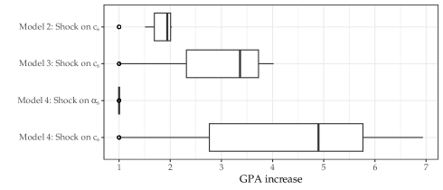
Figure 2: Effects of Shocks on the GPA

This figure presents the distribution of the increase in the GPA subsequent to a one-unit increase in $\alpha_{s}$ and $\delta^{2}c_{s}$ for the student sample (n = 68,430). Since $\delta$ is not identified, the shock on $c_{s}$ is scaled by $\delta^{2}$ because the parameter $c_{s}$ in our specification (9) is multiplied by $\delta^{2}$. However, it is important to note that regardless of the value of $\delta$, increasing $\alpha_{s}$ will still have the same influence on all students, whereas the implication of an increase in $c_{s}$ will vary depending on centrality.

4.4 Excluding Isolated Students

We next examine the performance of the various models estimated above when we exclude isolated students from our analysis. Note that in our main Add Health sample, 22% of the students have not nominated any friends. Among them, half (11% of the full sample) are not fully isolated, meaning they are nominated as friends by others, while the other half is fully isolated, having neither nominated friends nor being nominated by others.

Excluding the 22% isolated students from the sample will result in missing values in the network dataset, because the 11% of students who are not fully isolated have been nominated as friends by others. As demonstrated by Boucher and Houndetoungan (2022), this can lead to biased estimates of peer effects. In contrast, the exclusion of the “fully isolated" students allows us to conduct a robustness analysis, as it does not involve a missing network data issue. We thus define a new subsample by excluding the “fully isolated" students from our main sample, resulting in a subsample comprising 61,183 students from 139 schools.

Results are presented in Table 3. The peer effect estimate using the structural model (Model 4) is slightly larger at 0.878 after excluding fully isolated students. Similarly, the estimates using the standard linear-in-means model are also higher at 0.561 (Model 2) and 0.788 (Model 3).

This robustness analysis indicates that the bias in the estimation of peer effects when using the standard approach persists even after removing fully isolated students. This is because removal of fully isolated students still leaves in the sample some students who did not nominate any friends but were nominated by others. If we remove these students as well (Model 2^′), we still find that the peer effect estimate using the standard approach is downward biased. This is likely because, as mentioned above, removal of the partially isolated students creates missing values in the network dataset.

Table 3: Estimation results after excluding isolated students

		Excluding fully isolated						Excluding no friends
		Model 2		Model 3		Model 4		Model 2′
		Coef	Sd Err	Coef	Sd Err	Coef	Sd Err	Coef	Sd Err
Peer Effects		$0.561$	$0.030$	$0.788$	$0.042$	$0.878$	$0.044$	$0.581$	$0.034$
Weak instrument F		160		100		105		112
Sargan test prob.		0.000		0.095		0.493		0.000
Number of schools		139		139		139		139
Number of students		61,183		61,183		61,183		53,529

• Models 2, 3, and 4 are estimated using the subsample excluding fully isolated students (students who nominate no friends and who have not been nominated by others), whereas Model 2^′ is estimated using the sample excluding all students who do not nominate any friends. Model 2 controls for unobserved school heterogeneity but do not include dummy variables capturing isolated students i.e., $\alpha_{s}=0$ and $c_{s}$ varies across schools). Model 3 includes a single fixed effect per school with a dummy variable capturing isolated students (i.e., $\alpha_{s}$ may not be zero but is constant across schools, whereas $c_{s}$ varies). Model 4 is our structural model. The columns "Coef" report the coefficient estimates followed by their corresponding standard errors in the columns "Sd Err". Full results with the estimates of the coefficients associated with other variables in Table B.1.

5   Extension to Endogenous Networks

5.1 Method

The fact that certain characteristics of students that are unobserved might influence both educational outcomes and their social connections calls into question the assumption of an exogenous network. For instance, a student’s IQ or level of extroversion are likely to affect both their GPA and their choice of friends. Because these student characteristics are typically not observed by the econometrician, they would not be included in $\mathbf{X}_{s}$ and would instead be captured by the error terms $\boldsymbol{\eta}_{s}$ and $\boldsymbol{\varepsilon}_{s}$, giving rise to an omitted variables bias (network endogeneity).

Specifically, Equation (9) can now be written as:

$$y_{s,i}=\kappa^{NI}_{s}\ell^{NI}_{s,i}+\kappa^{I}_{s}(1-\ell^{NI}_{s,i})+\mathbf{g}_{s,i}\mathbf{y}_{s}+\mathbf{x}^{\prime}_{s,i}\boldsymbol{\tilde{\beta}}+\mathbf{g}_{s,i}\mathbf{X}_{s}\boldsymbol{\tilde{\gamma}}+h_{s,i}+\tilde{v}_{s,i},$$ (10)

where $h_{s,i}$ captures missing variables correlated with GPA that may also explain link formation in the social network. Treating the problem of network endogeneity as an omitted variables problem is a common approach in the literature (Goldsmith-Pinkham and Imbens, 2013; Hsieh and Lee, 2016; Johnsson and Moon, 2021; Jochmans, 2023). To address this problem, we rely on a two-stage method similar to the control function approach proposed by Johnsson and Moon (2021). We first estimate the omitted factors using a network formation model. In the second stage, we add them to our model as additional explanatory variables.

We consider a network formation model with degree heterogeneity (see Graham, 2017; Dzemski, 2019; Yan et al., 2019). In this model, the conditional probability of observing a link from student $i$ to student $j$ (that is, $i$ declares that $j$ is a friend) within the same school $s$ is denoted as

$$\mathbb{P}(a_{s,ij}=1|\ddot{\mathbf{x}}_{s,ij},\mu_{s,i}^{out},\mu_{s,j}^{in})=\Phi(\ddot{\mathbf{x}}_{s,ij}^{\prime}\ddot{\boldsymbol{\beta}}+\mu_{s,i}^{out}+\mu_{s,j}^{in}),$$ (11)

where $\Phi$ is either the normal or logistic distribution function, depending on whether the model follows a probit or logit specification; $\ddot{\mathbf{x}}_{s,ij}$ is a vector of observed dyad-specific variables, such as the distance between the characteristics of students $i$ and $j$, which influence the probability of forming a friendship link; $\mu_{s,i}^{out}$ and $\mu_{s,j}^{in}$ account for unobserved heterogeneity affecting student $i$’s likelihood of initiating friendships (outdegree) and student $j$’s likelihood of receiving friendship nominations (indegree), respectively. For instance, a student with a high IQ may be nominated as a friend by many classmates, resulting in a large indegree $\mu_{s,i}^{in}$. However, because the network is directed, this student’s outdegree can be low, if $\mu_{s,i}^{out}$ is low.

In Equation (11), there are more than $2n_{s}$ parameters to be estimated per school. However, Yan et al. (2019) show that the standard logit estimators of $\mu_{s,i}^{out}$ and $\mu_{s,j}^{in}$ are consistent if the network is dense. In this logit model, $\mu_{s,i}^{out}$ and $\mu_{s,j}^{in}$ are treated as fixed effects, that is, they can be correlated to the observed dyad-specific variables. We refer the interested reader to Yan et al. (2019) for a formal discussion of the model, including its identification and consistent estimation. Alternatively, a Bayesian probit model based on the data augmentation technique can be used to simulate the posterior distributions of $\mu_{s,i}^{out}$ and $\mu_{s,j}^{in}$ (see Albert and Chib, 1993). However, this approach treats $\mu_{s,i}^{out}$ and $\mu_{s,j}^{in}$ as random effects.

As in Johnsson and Moon (2021) and Houndetoungan (2022), we use a nonparametric approach to connect $h_{s,i}$ in Equation (10) to the unobserved factors $\mu_{s,i}^{out}$ and $\mu_{s,i}^{in}$. We impose that $h_{s,i}=h^{out}(\mu_{s,i}^{out})+h^{in}(\mu_{s,i}^{in})$, where $h^{out}$ and $h^{in}$ are continuous functions. This specification is more flexible than the assumption that $h_{s,i}$ is a linear function of $\mu_{s,i}^{out}$ and $\mu_{s,i}^{in}$, as imposed by Goldsmith-Pinkham and Imbens (2013) and Hsieh and Lee (2016). We approximate $h^{out}$ and $h^{in}$ using cubic B-splines as in generalized additive models (Hastie, 2017). The key idea behind this approach stems from the Weierstrass theorem, which states that any continuous function defined on a compact interval can be well approximated using polynomials. Specifically, we approximate $h^{out}(\mu_{s,i}^{out})$ by cubic polynomials on ten different intervals covering the range of $\mu_{s,i}^{out}$. The intervals are defined so that each comprises approximately the same share of observations. We also apply this approach to $h^{in}(\mu_{s,i}^{in})$. Given the number of intervals and the degree of the polynomials, this approach results in approximating $h_{s,i}$ by a combination of 26 variables, called bases, that are computed from the estimates of $\mu_{s,i}^{out}$ and $\mu_{s,i}^{in}$.

In the second stage, we use these new 26 variables as additional explanatory variables in the GPA model. Note that our identification analysis outlined in Section 3.2 is also valid here, under the assumption that $\mu_{s,i}^{out}$ and $\mu_{s,i}^{in}$ are well identified in the first stage. In contrast, achieving asymptotic normality in this two-stage estimation process becomes more complicated and cannot be generalized without new restrictions. In general, one needs the first-stage estimator to converge as fast as possible so that its approximation error does not influence the second-stage estimator asymptotically (see Online Appendix (OA) C.4). Alternatively, a bootstrap approach can be used to approximate the asymptotic distribution of the second-stage estimator.

5.2 Empirical Results

Table 4 presents the estimation results of peer effects, accounting for network endogeneity. Full results, including coefficients associated with other variables, can be found in Appendix B. We explore two approaches for estimating the unobserved factors $\mu_{i}^{out}$ and $\mu_{i}^{in}$: a fixed effects logit model (Models 2a, 3a, and 4a) and a random effects Bayesian model (Models 2b, 3b, and 4b). In all specifications, the new 26 regressors are globally significant, indicating the endogeneity of the network (we do not present the estimates for these new regressors).

In our preferred specifications (models 4a and 4b), the endogeneity does not significantly affect the estimate of peer effects. This result aligns with many other findings on the Add Health data arguing that the endogeneity of the network does not involve a substantial bias in the peer effects (e.g., Hsieh and Lee, 2016; Hsieh and Lin, 2017). Similar to those studies, we observe a slight decrease in the peer effect estimate (from 0.856 to 0.828). This decline occurs because of unobserved factors such as IQ that are positively correlated with GPA. For instance, an exogenous shock to IQ would simultaneously influence both students’ and peers’ GPAs. Accounting for the endogeneity helps disentangle true peer effects from these co-movements in GPA.

In the standard models (Models 2a and 2b), controlling for network endogeneity through the fixed effect approach significantly increases the peer effect estimate from 0.507 to 0.672. This control also mitigates the overidentification problem. The Sargan test probability increases from 0.000 to 0.039. Overidentification can occur due to the endogeneity of the network, which is likely to be the case in the standard model because the error term includes dummy variables for isolated students. By accounting for network endogeneity, the bias stemming from the omission of these variables is reduced. However, the Bayesian random effect approach still yields biased estimates. This is because this method only captures unobserved factors $\mu_{i}^{out}$ and $\mu_{i}^{in}$ that are independent of the regressions in $\mathbf{x}_{s,i}$. For example, this approach cannot control for the omission of the IQ because the latter would be corrected with $\mathbf{x}_{s,i}$. For the standard models with a dummy variable for isolated students (Model 3a, 3b), controlling for network endogeneity does not significantly influence the peer effects. Nonetheless, it effectively resolves the issue of overidentification.

Table 4: Estimation results controlling for network endogeneity

		Model 2a		Model 2b		Model 3a		Model 3B		Model 4a		Model 4b
		Coef	Sd Err	Coef	Sd Err	Coef	Sd Err	Coef	Sd Err	Coef	Sd Err	Coef	Sd Err
Peer Effects		$0.672$	$0.036$	$0.478$	$0.029$	$0.729$	$0.042$	$0.717$	$0.042$	$0.828$	$0.044$	$0.826$	$0.044$
Weak instrument F		131		190		113		113		114		114
Sargan test prob.		0.039		0.000		0.076		0.090		0.447		0.453
Number of schools		141		141		141		141		141		141
Number of students		68,430		68,430		68,430		68,430		68,430		68,430

• Models 2a, 3a, and 4a use logit fixed effects estimations for $\mu_{s,i}^{out}$ and $\mu_{s,i}^{in}$ in the first stage, whereas Models 2b, 3b, and 4c consider a Bayesian probit random effects estimate. In Models 2a and 2b, unobserved school heterogeneity is controlled for, but dummy variables capturing isolated students are not included ($\alpha_{s}=0$ and $c_{s}$ varies across schools). Models 3a and 3b include a single fixed effect per school with a dummy variable capturing isolated students (i.e., $\alpha_{s}$ may not be zero but is constant across schools, whereas $c_{s}$ varies). Models 4a and 4b are specified according to our structural model. The columns "Coef" report the coefficient estimates followed by their corresponding standard errors in the "Sd Err" columns. Full results with the estimates of the coefficients associated with other variables are presented in Appendix Table B.2.

6   Conclusion

This paper proposes a peer effect model in which students choose their level of academic effort, which in turn impacts their academic achievement (GPA). Unlike standard models used in the literature to estimate peer effects on GPA, our structural model accounts for two types of common shocks at the school level and allows for identifying peer effects on effort itself, even though effort is unobserved. We introduce common shocks that directly influence GPA, irrespective of effort levels, and common shocks affecting both students’ effort and their GPA.

We show that these two types of shocks have different impacts on GPA. Shocks exerted directly on GPA without influencing academic effort do not involve a social multiplier, whereas preference shocks that affect both academic effort and GPA may involve a social multiplier effect. We also show that failure to differentiate the two types of shocks results in a biased estimate of peer effects, when there are isolated students. Practically, accounting for the difference between the shocks amounts to controlling for student heterogeneity on the basis of whether they have friends or not.

Our model leads to an econometric specification that poses identification challenges. This occurs in particular because of the presence of unobserved school heterogeneity and students with no peers in the network. We derive conditions for identification and propose a multi-stage estimation strategy that combines the GMM and QML approaches. Our approach yields a consistent estimator, and we establish asymptotic normality. We also extend the estimation strategy and examine the case of endogenous networks.

We present an empirical illustration using Add Health data. We find that increasing the average GPA of peers by one point results in a 0.856 point increase in a student’s GPA. The peer effect estimate obtained using standard models is 40% lower than that obtained from our proposed approach. Controlling for network endogeneity in the standard models reduces the bias.

More generally, our framework can be used to study peer effects on activities that cannot be directly observed. An example is body mass index (BMI), which cannot be directly chosen. People need to exert effort, such as developing healthy diet habits, engaging in physical exercise, and avoiding fast food, to improve their BMI. Peer influence is more related to effort than BMI. Another example is peer effects on workers’ effort. The observed outcome is generally worker’s productivity, whereas peer effects stem from effort.

Appendix A Appendix: Proofs

A.1 Uniqueness of the Nash Equilibrium

By replacing the GPA with its expression given by Equation (1), we obtain a new payoff function $\hat{u}_{s,i}(e_{s,i},\mathbf{e}_{s,-i})$ that does not depend on the GPA. The new payoff function is

$$\textstyle\hat{u}_{s,i}(e_{s,i},\mathbf{e}_{s,-i})=(c_{s}+\mathbf{x}_{s,i}^{\prime}\boldsymbol{\beta}+\mathbf{g}_{s,i}\mathbf{X}_{s}\boldsymbol{\gamma}+\varepsilon_{s,i})(\alpha_{s}+\mathbf{x}^{\prime}_{s,i}\boldsymbol{\theta}+\delta e_{s,i}+\eta_{s,i})-\frac{e_{s,i}^{2}}{2}+\lambda e_{s,i}\mathbf{g}_{s,i}\mathbf{e}_{s}.$$ (A.1)

The first-order condition of the maximization of $\hat{u}_{s,i}(e_{s,i},\mathbf{e}_{s,-i})$ with respect to the effort $e_{s,i}$ gives

$$e_{s,i}=\delta c_{s}+\lambda\mathbf{g}_{s,i}\mathbf{e}_{s}+\delta\mathbf{x}_{s,i}^{\prime}\boldsymbol{\beta}+\delta\mathbf{g}_{s,i}\mathbf{X}_{s}\boldsymbol{\gamma}+\delta\varepsilon_{s,i}.$$ (A.2)

If we write Equation (A.2) at the school level, we get the best response functions of all students:

$$\mathbf{e}_{s}=\delta c_{s}\mathbf{1}_{n_{s}}+\lambda\mathbf{G}_{s}\mathbf{e}_{s}+\delta\mathbf{X}_{s}\boldsymbol{\beta}+\delta\mathbf{G}_{s}\mathbf{X}_{s}\boldsymbol{\gamma}+\delta\boldsymbol{\varepsilon}_{s},$$ (A.3)

where $\mathbf{1}_{n_{s}}$ is an $n_{s}$-vector of ones and $\boldsymbol{\varepsilon}_{s}=(\varepsilon_{s,1},\dots,\varepsilon_{s,n_{s}})^{\prime}$. Equation (A.3) is a system of $n_{s}$ linear equations in the effort. This system has a unique solution if $\lvert\mathbf{I}_{n_{s}}-\lambda\mathbf{G}_{s}\rvert\neq 0$, where $\mathbf{I}_{n_{s}}$ is the $n_{s}\times n_{s}$ identity matrix. The condition $\lvert\mathbf{I}_{n_{s}}-\lambda\mathbf{G}_{s}\rvert\neq 0$ is equivalent to saying that $1$ is not an eigenvalue for $\lambda\mathbf{G}_{s}$. As $\mathbf{G}_{s}$ is a row-normalized matrix, the eigenvalues of $\lambda\mathbf{G}_{s}$ are in the closed interval $[-\lvert\lambda\rvert,\leavevmode\nobreak\ \lvert\lambda\rvert]$. Thus, if $\lvert\lambda\rvert<1$, then $\lvert\mathbf{I}_{n_{s}}-\lambda\mathbf{G}_{s}\rvert\neq 0$ and the solution of Equation (A.3) is

$$\mathbf{e}_{s}=(\mathbf{I}_{n_{s}}-\lambda\mathbf{G}_{s})^{-1}(\delta c_{s}\mathbf{1}_{n_{s}}+\delta\mathbf{X}_{s}\boldsymbol{\beta}+\delta\mathbf{G}_{s}\mathbf{X}_{s}\boldsymbol{\gamma}+\delta\boldsymbol{\varepsilon}_{s}).$$ (A.4)

As a result, the game described by the payoff function (A.1) has a unique NE given by (A.4).

A.2 Reduced form equation of the GPA

Let $\boldsymbol{\eta}_{s}=(\eta_{s,1},\dots,\eta_{s,n_{s}})^{\prime}$ be the vector of the idiosyncratic error terms in Equation (1). Let also $\mathbf{y}_{s}=(y_{s,1},\dots,y_{s,n_{s}})^{\prime}$ be the GPAs’ vector. From Equation (1), we have $e_{s,i}=(y_{s,i}-\alpha_{s}-\mathbf{x}^{\prime}_{s,i}\boldsymbol{\theta}-\eta_{s,i})/\delta$. By replacing this expression in Equation (A.2), we get

$$\frac{y_{s,i}-\alpha_{s}-\mathbf{x}^{\prime}_{s,i}\boldsymbol{\theta}-\eta_{s,i}}{\delta}=\frac{\lambda\mathbf{g}_{s,i}(\mathbf{y}_{s}-\alpha_{s}\mathbf{1}_{n_{s}}-\mathbf{X}_{s}\boldsymbol{\theta}-\boldsymbol{\eta}_{s})}{\delta}+\delta(c_{s}+\mathbf{x}_{s,i}^{\prime}\boldsymbol{\beta}+\mathbf{g}_{s,i}\mathbf{X}_{s}\boldsymbol{\gamma}+\varepsilon_{s,i}),$$

$$y_{s,i}=\kappa_{s,i}+\lambda\mathbf{g}_{s,i}\mathbf{y}_{s}+\mathbf{x}^{\prime}_{s,i}\boldsymbol{\tilde{\beta}}+\mathbf{g}_{s,i}\mathbf{X}_{s}\boldsymbol{\tilde{\gamma}}+(\boldsymbol{\omega}_{s,i}-\lambda\mathbf{g}_{s,i})\boldsymbol{\eta}_{s}+\delta^{2}\varepsilon_{s,i},$$

where $\kappa_{s,i}=\delta^{2}c_{s}+(1-\lambda\mathbf{g}_{s,i}\mathbf{1}_{n_{s}})\alpha_{s}$, $\boldsymbol{\tilde{\beta}}=\delta^{2}\boldsymbol{\beta}+\boldsymbol{\theta}$, $\boldsymbol{\tilde{\gamma}}=\delta^{2}\boldsymbol{\gamma}-\lambda\boldsymbol{\theta}$, and $\boldsymbol{\omega}_{s,i}$ is a row-vector of dimension $n_{s}$ in which all the elements are equal to zero except the $i$-th element, which is one.

A.3 Proof of Proposition 3.1

We show that the reflection problem is addressed under Conditions (i) and (ii) of Assumption 3.2. Assume that $\mathbb{E}(\mathbf{J}_{s}\mathbf{G}_{s}\mathbf{y}_{s}|\mathbf{G}_{s},\mathbf{X}_{s})$ is perfectly collinear with $\mathbf{J}_{s}\mathbf{X}_{s}$ and $\mathbf{J}_{s}\mathbf{G}_{s}\mathbf{X}_{s}$. For any $i\in\mathcal{V}^{NI}_{s}$, we have $\mathbb{E}(\mathbf{g}_{s,i}\mathbf{y}_{s}-y^{NI}_{s}|\mathbf{G}_{s},\mathbf{X}_{s})=(\mathbf{x}_{s,i}^{\prime}-\mathbf{x}^{NI\prime}_{s})\dot{\boldsymbol{\beta}}+(\mathbf{g}_{s,i}\mathbf{X}_{s}^{\prime}-\bar{\mathbf{x}}^{NI\prime}_{s})\dot{\boldsymbol{\gamma}}$, where $y^{NI}_{s}$, $\mathbf{x}^{NI}_{s}$, and $\bar{\mathbf{x}}^{NI}_{s}$ are the respectively averages of $\mathbf{g}_{s,i}\mathbf{y}_{s}$, $\mathbf{x}_{s,i}$, and $(\mathbf{g}_{s,i}\mathbf{X}_{s})^{\prime}$ within $\mathcal{V}^{NI}_{s}$, and $\dot{\boldsymbol{\beta}}$, $\dot{\boldsymbol{\gamma}}$ are unknown parameters. The variables $\mathbf{g}_{s,i}\mathbf{y}_{s}$, $\mathbf{x}_{s,i}$, and $\mathbf{g}_{s,i}\mathbf{X}_{s}$ are taking in deviation with respect to their average in $\mathcal{V}^{NI}_{s}$ because of the matrix $\mathbf{J}_{s}$ that multiplies the terms of Equation (7). Let us take the previous equation in difference between two students $i_{1}$, $j$ from $\mathcal{V}^{NI}_{s}$, where $j$ is $i_{1}$’s friend. This implies:

$$\bar{y}^{e}_{s,i_{1}}-\bar{y}^{e}_{s,j}=(\mathbf{x}_{s,i_{1}}^{\prime}-\mathbf{x}_{s,j}^{\prime})\dot{\boldsymbol{\beta}}+(\bar{\mathbf{x}}_{s,i_{1}}^{\prime}-\bar{\mathbf{x}}_{s,j}^{\prime})\dot{\boldsymbol{\gamma}},$$ (A.5)

where $\bar{y}^{e}_{s,i}=\mathbb{E}(\mathbf{g}_{s,i}\mathbf{y}_{s}|\mathbf{G}_{s},\mathbf{X}_{s})$ and $\bar{\mathbf{x}}_{s,i}^{\prime}=\mathbf{g}_{s,i}\mathbf{X}_{s}$ for all $i$. Assume an increase in $\mathbf{x}_{l}$ for all $l$ that is separated from $i_{1}$ by a link of distance three, ceteris paribus. Such an $l$ exists by Condition (ii) of Assumption 3.2. As $j$ is $i_{1}$’s friend, $l$ cannot be $j$’s friend, otherwise, it would be possible to find a link of distance two from $l$ to $i_{1}$. Thus, an increase in any $\mathbf{x}_{l}$ has no influence on $\mathbf{x}_{s,i_{1}}^{\prime}$, $\mathbf{x}_{s,j}^{\prime}$, $\bar{\mathbf{x}}_{s,i_{1}}^{\prime}$, and $\bar{\mathbf{x}}_{s,j}^{\prime}$. Therefore, the right-hand side (RHS (A.5) would not be influenced and we would have

$$\Delta^{l}\bar{y}^{e}_{s,i_{1}}-\Delta^{l}\bar{y}^{e}_{s,j}=0,$$ (A.6)

where the operator $\Delta^{l}$ measures the variation after the increase in $\mathbf{x}_{l}$.

Using a proof by contradiction, we will now show that the condition $\Delta^{l}\bar{y}^{e}_{s,i_{1}}=\Delta^{l}\bar{y}^{e}_{s,j}$ for all $j$ who is $i_{1}$’s friend is not possible. By applying the operator $\Delta^{l}$ to every term of Equation (6), we have $\Delta^{l}\mathbf{y}_{s}=\lambda\mathbf{G}_{s}(\Delta^{l}\mathbf{y}_{s})+(\Delta^{l}\mathbf{X}_{s})\boldsymbol{\tilde{\beta}}+\mathbf{G}_{s}(\Delta^{l}\mathbf{X}_{s})\boldsymbol{\tilde{\gamma}}$. This implies that $\Delta^{l}\mathbf{y}_{s}=(\mathbf{I}-\lambda\mathbf{G}_{s})^{-1}\big{(}(\Delta^{l}\mathbf{X}_{s})\boldsymbol{\tilde{\beta}}+\mathbf{G}_{s}(\Delta^{l}\mathbf{X}_{s})\boldsymbol{\tilde{\gamma}}\big{)}$. As $(\mathbf{I}-\lambda\mathbf{G}_{s})^{-1}=\sum_{k=0}^{\infty}\lambda^{k}\mathbf{G}_{s}^{k}$, we can also write

$$\textstyle\Delta^{l}\mathbf{y}_{s}=(\Delta^{l}\mathbf{X}_{s})\boldsymbol{\tilde{\beta}}+\sum_{k=0}^{\infty}\lambda^{k}\mathbf{G}_{s}^{k+1}(\Delta^{l}\mathbf{X}_{s})(\lambda\boldsymbol{\tilde{\beta}}+\boldsymbol{\tilde{\gamma}}).$$ (A.7)

Equation (A.7) implies the GPA is influenced by the contextual variables if and only if $\lambda\boldsymbol{\tilde{\beta}}+\boldsymbol{\tilde{\gamma}}\neq 0$.
By premultiplying (A.7) by $\mathbf{g}_{s,i_{1}}$ and taking the expectation conditional on $\mathbf{G}_{s}$ and $\mathbf{X}_{s}$, we have

$$\textstyle\Delta^{l}\bar{y}^{e}_{s,i_{1}}=\mathbf{g}_{s,i_{1}}\sum_{k=1}^{\infty}\lambda^{k}\mathbf{G}_{s}^{k+1}(\Delta^{l}\mathbf{X}_{s})(\lambda\boldsymbol{\tilde{\beta}}+\boldsymbol{\tilde{\gamma}}).$$ (A.8)

Indeed $\mathbf{g}_{s,i_{1}}(\Delta^{l}\mathbf{X}_{s})=0$ and $\mathbf{g}_{s,i_{1}}\mathbf{G}_{s}(\Delta^{l}\mathbf{X}_{s})=0$ (since $l$ is separated from $i_{1}$ by a link of distance three, $l$ is not $i_{1}$’s friend, nor $i_{1}$’s friend’s friend).

By premultiplying each term of Equation (A.7) by $\lambda\mathbf{G}_{s}$, we obtain $\sum_{k=1}^{\infty}\lambda^{k}\mathbf{G}_{s}^{k+1}(\Delta^{l}\mathbf{X}_{s})(\lambda\boldsymbol{\tilde{\beta}}+\boldsymbol{\tilde{\gamma}})=\lambda\mathbf{G}_{s}\Delta^{l}\mathbf{y}_{s}-\lambda\mathbf{G}_{s}(\Delta^{l}\mathbf{X}_{s})\boldsymbol{\tilde{\beta}}$. By replacing the previous equation in (A.8), we get

$$\Delta^{l}\bar{y}^{e}_{s,i_{1}}=\lambda\mathbf{g}_{s,i_{1}}\mathbf{G}_{s}\Delta^{l}\mathbf{y}_{s},$$ (A.9)

because $\mathbf{g}_{s,i_{1}}\mathbf{G}_{s}(\Delta^{l}\mathbf{X}_{s})=0$. As $\mathbf{G}_{s}\Delta^{l}\mathbf{y}_{s}=(\Delta^{l}\bar{y}^{e}_{s,1},\dots,\Delta^{l}\bar{y}^{e}_{s,n_{s}})^{\prime}$, the term $\mathbf{g}_{s,i_{1}}\mathbf{G}_{s}\Delta^{l}\mathbf{y}_{s}$ in the RHS of Equation (A.9) is the average of $\Delta^{l}\bar{y}^{e}_{s,j}$ among students $j$ who are $i_{1}$’s friends. If Equation (A.6) holds true, that is, if $\Delta^{l}\bar{y}^{e}_{s,j}=\Delta^{l}\bar{y}^{e}_{s,i_{1}}$ for any $j$ who is $i_{1}$’s friend, this would mean that $\mathbf{g}_{s,i_{1}}\mathbf{G}_{s}\Delta^{l}\mathbf{y}_{s}=\Delta^{l}\bar{y}^{e}_{s,i_{1}}$ and Equation (A.9) would imply that $\Delta^{l}\bar{y}^{e}_{s,i_{1}}=\lambda\Delta^{l}\bar{y}^{e}_{s,i_{1}}$. This is where the contradiction would come from. Indeed, the previous equation is not compatible with Equation (A.6) since $\lambda\neq 1$ by Assumption 2.1, and $\Delta^{l}\bar{y}^{e}_{s,i_{1}}\neq 0$ because $\lambda\boldsymbol{\tilde{\beta}}+\boldsymbol{\tilde{\gamma}}\neq 0$ (see Equation (A.7)). As a result, the model does not suffer from the reflection problem.

Let $\mathbf{\tilde{X}}_{s}=\mathbf{J}_{s}[\mathbf{X}_{s},\leavevmode\nobreak\ \mathbf{G}_{s}\mathbf{X}_{s}]$, $\mathbf{R}_{s}=[\mathbf{J}_{s}\mathbf{G}_{s}\mathbf{y}_{s},\leavevmode\nobreak\ \mathbf{\tilde{X}}_{s}]$, $\mathbf{Z}_{s}=[\mathbf{J}_{s}\mathbf{G}_{s}^{2}\mathbf{X}_{s},\leavevmode\nobreak\ \mathbf{\tilde{X}}_{s}]$, $\mathbf{R}^{\prime}\mathbf{Z}=\sum_{s=1}^{S}\mathbf{R}^{\prime}_{s}\mathbf{Z}_{s}$, and $\mathbf{Z}^{\prime}\mathbf{Z}=\sum_{s=1}^{S}\mathbf{Z}^{\prime}_{s}\mathbf{Z}_{s}$. We set the following identification conditions.

Assumption A.1.

The matrices $\mathbf{R}^{\prime}\mathbf{Z}/n$ and $\mathbf{Z}^{\prime}\mathbf{Z}/n$ converge to full rank matrices as $S$ grows to infinity. Moreover, $\sum_{s=1}^{S}\mathbf{Z}_{s}^{\prime}((\mathbf{I}_{n_{s}}-\lambda\mathbf{G}_{s})\boldsymbol{\eta}_{s}++\delta^{2}\boldsymbol{\varepsilon}_{s})/n=o_{p}(1)$.

The first half of Assumption A.1 suggests that the columns of design matrix $\mathbf{R}=[\mathbf{R}^{\prime}_{1},\leavevmode\nobreak\ \dots,\mathbf{R}_{S}^{\prime}]^{\prime}$ and those of the instrument matrix $\mathbf{Z}=[\mathbf{Z}^{\prime}_{1},\leavevmode\nobreak\ \dots,\mathbf{Z}_{S}^{\prime}]^{\prime}$ are linearly independent for large $S$. The second condition of the assumption comes from the exogeneity of $\mathbf{X}_{s}$ and $\mathbf{G}_{s}$ with respect to $\boldsymbol{\eta}_{s}$ and $\varepsilon_{s}$. Under Assumptions 2.1, 3.1, 3.2, and A.1, the design matrix of Equation (7) is full rank for large $n$, and the identification of $\boldsymbol{\psi}$ follows.

A.4 Proof of Proposition 3.2

In this section, we use different notations for the parameters and their true values; that is their values in the data-generating process. We denote by $\boldsymbol{\psi}_{0}$, $\sigma_{0\eta}$, $\sigma_{0\epsilon}$, and $\rho_{0}$ the true values of $\boldsymbol{\psi}$, $\sigma_{\eta}$, $\sigma_{\epsilon}$, and $\rho$, respectively.

However, the log-likelihood cannot be written directly because the transformation we apply to eliminate the fixed effects $\kappa^{NI}_{s}$ and $\kappa^{I}_{s}$ makes the covariance matrix $\mathbb{E}(\boldsymbol{v}_{s}\boldsymbol{v}_{s}^{\prime}|\mathbf{G}_{s})$ singular (for example, we have $\mathbf{1}_{n_{s}}^{\prime}\boldsymbol{v}_{s}=0$). In other words, we cannot invert the covariance matrix $\mathbb{E}(\boldsymbol{v}_{s}\boldsymbol{v}_{s}^{\prime}|\mathbf{G}_{s})$, which is a necessary task to write the log-likelihood. To address this issue, we use a similar approach to that of Lee et al. (2010). Let $[\mathbf{F}_{s},\leavevmode\nobreak\ \boldsymbol{\ell}^{I}_{s}/\sqrt{n^{I}_{s}},\leavevmode\nobreak\ \boldsymbol{\ell}^{NI}_{s}/\sqrt{n^{NI}_{s}}]$ be the orthonormal matrix of $\mathbf{J}_{s}$, where the columns in $\mathbf{F}_{s}$ are eigenvectors of $\mathbf{J}_{s}$ corresponding to the eigenvalue one. To ease the notational burden, we assume the school $s$ has students in both $\mathcal{V}^{I}_{s}$ and $\mathcal{V}^{NI}_{s}$. We have $\mathbf{F}_{s}\mathbf{F}_{s}^{\prime}=\mathbf{J}_{s}$ and $\mathbf{F}_{s}^{\prime}\mathbf{F}_{s}=\mathbf{I}_{n_{s}-2}$. As $\mathbf{F}_{s}$ does not depend on unknown parameters, maximizing the log-likelihood of $\hat{\boldsymbol{v}}_{s}$ is equivalent to maximizing that of $\mathbf{F}_{s}^{\prime}\hat{\boldsymbol{v}}_{s}$. The log-likelihood of $\mathbf{F}_{s}^{\prime}\hat{\boldsymbol{v}}_{s}$ is given by

$$\textstyle\hat{L}(\sigma_{\eta}^{2},\sigma_{\epsilon}^{2},\rho)=-\sum_{s=1}^{S}\frac{n_{s}-2}{2}\log(\sigma_{\epsilon}^{2})-\frac{1}{2}\sum_{s=1}^{S}\log\lvert\boldsymbol{\Omega}_{s}(\hat{\lambda},\tau,\rho)\rvert-\sum_{s=1}^{S}\frac{1}{2\sigma_{\epsilon}^{2}}\hat{\boldsymbol{v}}_{s}^{\prime}\mathbf{F}_{s}\boldsymbol{\Omega}^{-1}_{s}(\hat{\lambda},\tau,\rho)\mathbf{F}_{s}^{\prime}\hat{\boldsymbol{v}}_{s},$$ (A.10)

where $\boldsymbol{\Omega}_{s}(\hat{\lambda},\tau,\rho)=\mathbf{I}_{n_{s}-2}+\tau^{2}\mathbf{F}_{s}^{\prime}\mathbf{W}_{s}\mathbf{W}_{s}^{\prime}\mathbf{F}_{s}+\rho\tau\mathbf{F}_{s}^{\prime}(\mathbf{W}_{s}+\mathbf{W}_{s}^{\prime})\mathbf{F}_{s}$, $\mathbf{W}_{s}=\mathbf{I}_{n_{s}}-\hat{\lambda}\mathbf{G}_{s}$, and $\tau=\sigma_{\eta}/\sigma_{\epsilon}$. The first-order conditions of the maximization of (A.10) imply that $\sigma_{\epsilon}^{2}$ can be substituted with $\tilde{\sigma}_{\epsilon}^{2}(\tau,\rho)=\sum_{s=1}^{S}\frac{\hat{\boldsymbol{v}}_{s}^{\prime}\mathbf{F}_{s}\boldsymbol{\Omega}^{-1}_{s}(\hat{\lambda},\tau,\rho)\mathbf{F}_{s}^{\prime}\hat{\boldsymbol{v}}_{s}}{n-2S}$. This leads to a simpler concentrated log-likelihood that does not depend on $\sigma_{\epsilon}^{2}$ and is easier to maximize. We also define the following log-likelihood by replacing $\hat{\boldsymbol{v}}_{s}$ and $\hat{\lambda}$ in $\hat{L}(\sigma_{\eta}^{2},\sigma_{\epsilon}^{2},\rho)$ with their true value:

$$\textstyle L(\sigma_{\eta}^{2},\sigma_{\epsilon}^{2},\rho)=-\sum_{s=1}^{S}\frac{n_{s}-2}{2}\log(\sigma_{\epsilon}^{2})-\frac{1}{2}\sum_{s=1}^{S}\log\lvert\boldsymbol{\Omega}_{s}(\lambda_{0},\tau,\rho)\rvert-\sum_{s=1}^{S}\frac{1}{2\sigma_{\epsilon}^{2}}\boldsymbol{v}_{s}^{\prime}\mathbf{F}_{s}\boldsymbol{\Omega}^{-1}_{s}(\lambda_{0},\tau,\rho)\mathbf{F}_{s}^{\prime}\boldsymbol{v}_{s},$$

where $\boldsymbol{v}_{s}=\mathbf{J}_{s}(\mathbf{I}_{n_{s}}-\lambda_{0}\mathbf{G}_{s})\boldsymbol{\eta}_{s}+\delta^{2}\mathbf{J}_{s}\boldsymbol{\varepsilon}_{s}$. Let $\pi_{\min}(.)$ be the smallest eigenvalue and $\pi_{\max}(.)$ be the largest eigenvalue. The operator $\lVert.\rVert_{2}$ applied to a matrix is the operator norm induced by the $\ell^{2}$-norm. We also denote by $\boldsymbol{\Theta}$ the space of $(\sigma_{\eta}^{2},\leavevmode\nobreak\ \sigma_{\epsilon}^{2},\leavevmode\nobreak\ \rho)$.

The proof is done in several steps.

Step 1

We show that $\frac{1}{n-2S}(\hat{L}(\sigma_{\eta}^{2},\sigma_{\epsilon}^{2},\rho)-L(\sigma_{\eta}^{2},\sigma_{\epsilon}^{2},\rho))$ converges in probability to zero uniformly in $\boldsymbol{\Theta}$. This proof would imply that we can focus on $L(\sigma_{\eta}^{2},\sigma_{\epsilon}^{2},\rho)$ for the identification and consistency instead of $\hat{L}(\sigma_{\eta}^{2},\sigma_{\epsilon}^{2},\rho)$. To do so, we set the following assumptions.

Assumption A.2.

(i) $\boldsymbol{\Theta}$is a compact subset of $\mathbb{R}^{3}$ and (ii) $\lim_{S\to\infty}\pi_{\min}(\boldsymbol{\Omega}_{s}(\hat{\lambda},\tau,\rho))>0$for any $s$.

Assumption A.3.

(i) $\mathbb{E}(\eta_{s,i}^{4}|\mathbf{G}_{s},\mathbf{X}_{s})$, $\mathbb{E}(\varepsilon_{s,i}^{4}|\mathbf{G}_{s},\mathbf{X}_{s})$, and $\mathbb{E}(\eta_{s,i}^{2}\varepsilon_{s,i}^{2}|\mathbf{G}_{s},\mathbf{X}_{s})$ exist; (ii) $\max_{s,i}\lvert\eta_{s,i}\rvert=O_{p}(1)$, $\max_{s,i}\lvert\varepsilon_{s,i}\rvert=O_{p}(1)$, and $\max_{s,i}\lVert\mathbf{x}_{s,i}\rVert_{2}=O_{p}(1)$.

Condition (i) of Assumption A.2 is required in many econometric models. It allows for generalizing pointwise convergences to uniform convergences. Condition (ii) of Assumption A.2 generalizes the nonsingularity of the matrix $\boldsymbol{\Omega}_{s}(\hat{\lambda},\tau,\rho)$ to large samples (when $S$ grows to infinity). Assumption A.3 sets further conditions regarding the distribution of $(\eta_{s,i},\leavevmode\nobreak\ \varepsilon_{s,i})^{\prime}$ and ensures that $\mathbf{x}_{s,i}$ and the $i$-th component of $\boldsymbol{v}_{s}$ are bounded.

Because $\mathbf{G}_{s}$ is row-normalized and bounded in column sum (Assumption 3.3), then for all $\tau$ and $\rho$, $\boldsymbol{\tilde{\Omega}}_{s}(\hat{\lambda},\tau,\rho):=\mathbf{I}_{n_{s}}+\tau^{2}\mathbf{W}_{s}\mathbf{W}_{s}^{\prime}+\rho\tau(\mathbf{W}_{s}+\mathbf{W}_{s}^{\prime})$ is also absolutely bounded in both row and column sums, and $\pi_{\max}(\boldsymbol{\tilde{\Omega}}_{s}(\hat{\lambda},\tau,\rho))<\infty$. Moreover, as $\boldsymbol{\Omega}_{s}(\hat{\lambda},\tau,\rho)=\mathbf{F}_{s}^{\prime}\boldsymbol{\tilde{\Omega}}_{s}(\hat{\lambda},\tau,\rho)\mathbf{F}_{s}$, we have $\pi_{\max}(\boldsymbol{\Omega}_{s}(\hat{\lambda},\tau,\rho))\leq\pi_{\max}(\boldsymbol{\tilde{\Omega}}_{s}(\hat{\lambda},\tau,\rho))<\infty$. Thus, $\frac{1}{n-2S}\sum_{s=1}^{S}\log\lvert\boldsymbol{\Omega}_{s}(\hat{\lambda},\tau,\rho)\rvert<\infty$ for all $\sigma_{\eta}^{2}$, $\sigma_{\epsilon}^{2}$, and $\rho$. As a result, $\frac{1}{n-2S}\sum_{s=1}^{S}\log\lvert\boldsymbol{\Omega}_{s}(\hat{\lambda},\tau,\rho)\rvert-\frac{1}{n-2S}\sum_{s=1}^{S}\log\lvert\boldsymbol{\Omega}_{s}(\lambda_{0},\tau,\rho)\rvert=o_{p}(1)$ (because the determinant is continuous).

Besides, $\hat{\boldsymbol{v}}_{s}=\boldsymbol{v}_{s}+\Delta\hat{\boldsymbol{v}}_{s}$, where $\Delta\hat{\boldsymbol{v}}_{s}=\mathbf{R}_{s}(\boldsymbol{\psi}_{0}-\boldsymbol{\hat{\psi}})$. As $\max_{s,i}\lVert\mathbf{x}_{s,i}\rVert_{2}=O_{p}(1)$ and $(\boldsymbol{\psi}_{0}-\boldsymbol{\hat{\psi}})=O_{p}(n^{-1/2})$, then each component of $\Delta\hat{\boldsymbol{v}}_{s}$ is $O_{p}(n^{-1/2})$ and $\lVert\Delta\hat{\boldsymbol{v}}_{s}\rVert_{2}=O_{p}((n_{s}/n)^{1/2})$. On the other hand, as $\max_{s,i}\lvert\eta_{s,i}\rvert=O_{p}(1)$ and $\max_{s,i}\lvert\varepsilon_{s,i}\rvert=O_{p}(1)$, we have $\lVert\boldsymbol{v}_{s}\rVert_{2}=O_{p}(n_{s}^{1/2})$. We also have

$$\hat{\boldsymbol{v}}_{s}^{\prime}\mathbf{F}_{s}\boldsymbol{\Omega}^{-1}_{s}(\hat{\lambda},\tau,\rho)\mathbf{F}_{s}^{\prime}\hat{\boldsymbol{v}}_{s}=\boldsymbol{v}_{s}^{\prime}\mathbf{F}_{s}\boldsymbol{\Omega}^{-1}_{s}(\hat{\lambda},\tau,\rho)\mathbf{F}_{s}^{\prime}\boldsymbol{v}_{s}+2\Delta\hat{\boldsymbol{v}}_{s}^{\prime}\mathbf{F}_{s}\boldsymbol{\Omega}^{-1}_{s}(\hat{\lambda},\tau,\rho)\mathbf{F}_{s}^{\prime}\boldsymbol{v}_{s}+\Delta\hat{\boldsymbol{v}}_{s}^{\prime}\mathbf{F}_{s}\boldsymbol{\Omega}^{-1}_{s}(\hat{\lambda},\tau,\rho)\mathbf{F}_{s}^{\prime}\Delta\hat{\boldsymbol{v}}_{s}.$$

The submultiplicativity property of the operator norm implies that $\sum_{s=1}^{S}\lvert\Delta\hat{\boldsymbol{v}}_{s}^{\prime}\mathbf{F}_{s}\boldsymbol{\Omega}^{-1}_{s}(\hat{\lambda},\tau,\rho)\mathbf{F}_{s}^{\prime}\boldsymbol{v}_{s}\rvert=O_{p}(n^{1/2})$ and $\sum_{s=1}^{S}\lvert\Delta\hat{\boldsymbol{v}}_{s}^{\prime}\mathbf{F}_{s}\boldsymbol{\Omega}^{-1}_{s}(\hat{\lambda},\tau,\rho)\mathbf{F}_{s}^{\prime}\Delta\hat{\boldsymbol{v}}_{s}\rvert=O_{p}(1)$ because $\lVert\mathbf{F}_{s}\rVert_{2}=1$ and $\lVert\boldsymbol{\Omega}^{-1}_{s}(\hat{\lambda},\tau,\rho)\rVert_{2}=O_{p}(1)$ (Assumption A.2). Thus, $\frac{1}{n-2S}(\hat{\boldsymbol{v}}_{s}^{\prime}\mathbf{F}_{s}\boldsymbol{\Omega}^{-1}_{s}(\hat{\lambda},\tau,\rho)\mathbf{F}_{s}^{\prime}\hat{\boldsymbol{v}}_{s}-\boldsymbol{v}_{s}^{\prime}\mathbf{F}_{s}\boldsymbol{\Omega}^{-1}_{s}(\hat{\lambda},\tau,\rho)\mathbf{F}_{s}^{\prime}\boldsymbol{v}_{s})=o_{p}(1)$. We also have $\frac{1}{n-2S}(\hat{\boldsymbol{v}}_{s}^{\prime}\mathbf{F}_{s}\boldsymbol{\Omega}^{-1}_{s}(\hat{\lambda},\tau,\rho)\mathbf{F}_{s}^{\prime}\hat{\boldsymbol{v}}_{s}-\boldsymbol{v}_{s}^{\prime}\mathbf{F}_{s}\boldsymbol{\Omega}^{-1}_{s}(\lambda_{0},\tau,\rho)\mathbf{F}_{s}^{\prime}\boldsymbol{v}_{s})=o_{p}(1)$ because $\boldsymbol{v}_{s}^{\prime}\mathbf{F}_{s}\boldsymbol{\Omega}^{-1}_{s}(\hat{\lambda},\tau,\rho)\mathbf{F}_{s}^{\prime}\boldsymbol{v}_{s}$ is a continuous function of $\hat{\lambda}$.
As a result, $\frac{1}{n}(\hat{L}(\sigma_{\eta}^{2},\sigma_{\epsilon}^{2},\rho)-L(\sigma_{\eta}^{2},\sigma_{\epsilon}^{2},\rho))=o_{p}(1)$. The convergence is uniform because the log-likelihoods can be expressed as a polynomial function in $(\sigma_{\eta}^{2},\leavevmode\nobreak\ \sigma_{\epsilon}^{2},\leavevmode\nobreak\ \rho)$. We can now focus on the log-likelihood $L(\sigma_{\eta}^{2},\sigma_{\epsilon}^{2},\rho)$ for the identification and the consistency of $(\sigma_{0\epsilon}^{2},\leavevmode\nobreak\ \tau_{0},\leavevmode\nobreak\ \rho_{0})$, where $\tau_{0}=\sigma_{0\eta}/\sigma_{0\epsilon}$.

Step 2

The first-order conditions (foc) of the maximization of $L(\sigma_{\eta}^{2},\sigma_{\epsilon}^{2},\rho)$ imply that $\sigma_{\epsilon}^{2}$ can be replaced with $\hat{\sigma}_{\epsilon}^{2}(\tau,\rho)=\sum_{s=1}^{S}\frac{\boldsymbol{v}_{s}^{\prime}\mathbf{F}_{s}\boldsymbol{\Omega}^{-1}_{s}(\lambda_{0},\tau,\rho)\mathbf{F}_{s}^{\prime}\boldsymbol{v}_{s}}{n-2S}$. This leads to a concentrated log-likelihood given by $\textstyle L_{c}(\tau,\rho)=-\frac{n-2S}{2}\hat{\sigma}_{\epsilon}^{2}(\tau,\rho)-\frac{1}{2}\sum_{s=1}^{S}\log\lvert\boldsymbol{\Omega}_{s}(\lambda_{0},\tau,\rho)\rvert-\frac{n-2S}{2}$ that does not depend on $\sigma_{\epsilon}^{2}$. Let $L^{\ast}(\sigma_{\eta}^{2},\sigma_{\epsilon}^{2},\rho)=\mathbb{E}\left(L(\sigma_{\eta}^{2},\sigma_{\epsilon}^{2},\rho)|\mathbf{G}_{1},\dots,\mathbf{G}_{S}\right)$. As for $L(\sigma_{\eta}^{2},\sigma_{\epsilon}^{2},\rho)$, we can also replace $\sigma_{\epsilon}^{2}$ with $\mathbb{E}\left(\hat{\sigma}_{\epsilon}^{2}(\tau,\rho)|\mathbf{G}_{1},\dots,\mathbf{G}_{S}\right)$.

$$\mathbb{E}(\hat{\sigma}_{\epsilon}^{2}(\tau,\rho)|\mathbf{G}_{1},\dots,\mathbf{G}_{S}) =\textstyle\frac{\sigma_{0\varepsilon}^{2}}{n-2S}\sum_{s=1}^{S}\mathbb{E}(\operatorname{Tr}(\boldsymbol{v}_{s}^{\prime}\mathbf{F}_{s}\boldsymbol{\Omega}^{-1}_{s}(\lambda_{0},\tau,\rho)\mathbf{F}_{s}^{\prime}\boldsymbol{v}_{s})|\mathbf{G}_{1},\dots,\mathbf{G}_{S}),$$

$$\mathbb{E}(\hat{\sigma}_{\epsilon}^{2}(\tau,\rho)|\mathbf{G}_{1},\dots,\mathbf{G}_{S}) =\textstyle\frac{\sigma_{0\varepsilon}^{2}}{n-2S}\sum_{s=1}^{S}\mathbb{E}(\operatorname{Tr}(\boldsymbol{\Omega}^{-1}_{s}(\lambda_{0},\tau,\rho)\mathbf{F}_{s}^{\prime}\boldsymbol{v}_{s}\boldsymbol{v}_{s}^{\prime}\mathbf{F}_{s})|\mathbf{G}_{1},\dots,\mathbf{G}_{S}),$$

$$\mathbb{E}(\hat{\sigma}_{\epsilon}^{2}(\tau,\rho)|\mathbf{G}_{1},\dots,\mathbf{G}_{S}) \textstyle=\frac{\sigma_{0\varepsilon}^{2}}{n-2S}\sum_{s=1}^{S}\operatorname{Tr}(\boldsymbol{\Omega}^{-1}_{s}(\lambda_{0},\tau,\rho)\mathbb{E}(\mathbf{F}_{s}^{\prime}\boldsymbol{v}_{s}\boldsymbol{v}_{s}^{\prime}\mathbf{F}_{s}|\mathbf{G}_{1},\dots,\mathbf{G}_{S})),$$

$$\mathbb{E}(\hat{\sigma}_{\epsilon}^{2}(\tau,\rho)|\mathbf{G}_{1},\dots,\mathbf{G}_{S}) \textstyle=\frac{\sigma_{0\varepsilon}^{2}}{n-2S}\sum_{s=1}^{S}\operatorname{Tr}(\boldsymbol{\Omega}^{-1}_{s}(\lambda_{0},\tau,\rho)\boldsymbol{\Omega}_{0,s}),$$ (A.11)

where $\boldsymbol{\Omega}_{0,s}=\boldsymbol{\Omega}_{s}(\lambda_{0},\tau_{0},\rho_{0})$.
We obtain the concentrated log-likelihood $\textstyle L_{c}^{\ast}(\tau,\rho)=-\frac{n-2S}{2}\tilde{\sigma}_{\epsilon}^{2\ast}(\tau,\rho)-\frac{1}{2}\sum_{s=1}^{S}\log\lvert\boldsymbol{\Omega}_{s}(\lambda_{0},\tau,\rho)\rvert-\frac{n-2S}{2},$ where $\tilde{\sigma}_{\epsilon}^{2\ast}(\tau,\rho)=\frac{\sigma_{0\varepsilon}^{2}}{n-2S}\sum_{s=1}^{S}\operatorname{Tr}\left(\boldsymbol{\Omega}^{-1}_{s}(\lambda_{0},\tau,\rho)\boldsymbol{\Omega}_{0,s}\right)$. We show that $\frac{1}{n}(L_{c}(\tau,\rho)-L_{c}^{\ast}(\tau,\rho))$ converges to zero uniformly.

Although $\mathbb{E}\left(\hat{\sigma}_{\epsilon}^{2}(\tau,\rho)|\mathbf{G}_{1},\dots,\mathbf{G}_{S}\right)=\tilde{\sigma}_{\epsilon}^{2\ast}(\tau,\rho)$, this does not implies that $\operatorname{plim}\hat{\sigma}_{\epsilon}^{2}(\tau,\rho)=\tilde{\sigma}_{\epsilon}^{2\ast}(\tau,\rho)$. We also need to show that the variance of $\hat{\sigma}_{\epsilon}^{2}(\tau,\rho)$ converges to zero as $S$ grows to infinity. This is especially important in our framework because the components of $\boldsymbol{v}_{s}$ are connected through the network and also because $n_{s}$ is not necessarily bounded. This is why we impose that fourth-order moments of $\eta_{s,i}$ and $\varepsilon_{s,i}$ exist in Assumption A.3. In fact, the variance of $\hat{\sigma}_{\epsilon}^{2}(\tau,\rho)$ involves up to the fourth power of the components of $\boldsymbol{v}_{s}$. We provide the proof in OA C.2. The uniform convergence of $\frac{1}{n}(L_{c}(\tau,\rho)-L_{c}^{\ast}(\tau,\rho))$ to zero directly follows.

Step 3

To establish the identification of the consistency, we need to show $L_{c}^{\ast}(\tau,\rho)$ is maximized at a single point which is $(\tau_{0},\leavevmode\nobreak\ \rho_{0})$ (see Newey and McFadden, 1994). We set the following assumption.

Assumption A.4.

If $(\tau,\rho)\neq(\tau_{0},\leavevmode\nobreak\ \rho_{0})$, then $\frac{\displaystyle\lim_{n\to\infty}\textstyle(\sum_{s=1}^{S}(\log\lvert\tilde{\sigma}_{\epsilon}^{2\ast}(\tau,\rho)\boldsymbol{\Omega}_{s}(\lambda_{0},\tau,\rho)\rvert-\log\lvert\sigma_{0\varepsilon}^{2}\boldsymbol{\Omega}_{0,s}\rvert)}{n}\neq 0$.

The intuition of Assumption A.4 is as follows. After replacing $\sigma_{\epsilon}^{2}$ with $\tilde{\sigma}_{\epsilon}^{2}(\tau,\rho)$ in Equation (A.10), the variable part of the concentrated log-likelihood is proportional to $\frac{1}{n}\sum_{s=1}^{S}\log\lvert\tilde{\sigma}_{\epsilon}^{2}(\tau,\rho)\boldsymbol{\Omega}_{s}(\hat{\lambda},\tau,\rho)\rvert$, which is asymptotically equivalent to $\frac{1}{n}\sum_{s=1}^{S}\log\lvert\tilde{\sigma}_{\epsilon}^{2\ast}(\tau,\rho)\boldsymbol{\Omega}_{s}(\hat{\lambda},\tau,\rho)\rvert$. Assumption A.4 implies that the value of $\frac{1}{n}\sum_{s=1}^{S}\log\lvert\tilde{\sigma}_{\epsilon}^{2\ast}(\tau,\rho)\boldsymbol{\Omega}_{s}(\hat{\lambda},\tau,\rho)\rvert$ at $(\tau_{0},\leavevmode\nobreak\ \rho_{0})$ cannot be reached at another point as $S$ grows to infinity. This assumption adapts Assumption 9 of Lee (2004) or Assumption 5.1 of Lee et al. (2010) to our framework.

Let $(\boldsymbol{e}_{s})_{s}$ be a process normally distributed of zero mean and covariance matrix $\sigma_{0\epsilon}^{2}\boldsymbol{\Omega}_{s}(\tau_{0},\leavevmode\nobreak\ \rho_{0})$. Let $L^{0}(\sigma_{\eta}^{2},\sigma_{\epsilon}^{2},\rho)=-\sum_{s=1}^{S}\frac{n_{s}-2}{2}\sigma_{\epsilon}^{2}-\frac{1}{2}\sum_{s=1}^{S}\log\lvert\boldsymbol{\Omega}_{s}(\lambda_{0},\tau,\rho)\rvert-\sum_{s=1}^{S}\frac{1}{2\sigma_{\epsilon}^{2}}\boldsymbol{e}_{s}^{\prime}\mathbf{F}_{s}\boldsymbol{\Omega}^{-1}_{s}(\lambda_{0},\tau,\rho)\mathbf{F}_{s}^{\prime}\boldsymbol{e}_{s}$. By Jensen’s inequality, we have $\operatorname{\mathbb{E}}(L^{0}(\sigma_{\eta}^{2},\sigma_{\epsilon}^{2},\rho)-L^{0}(\sigma_{0\eta}^{2},\sigma_{0\epsilon}^{2},\rho_{0})|\mathbf{G}_{1},\dots,\mathbf{G}_{S})\leq 0$. This suggests that $(\tau_{0},\leavevmode\nobreak\ \rho_{0})$ is a global maximizer of $\operatorname{plim}\frac{1}{n}L^{\ast}_{c}(\tau,\rho)$. The uniqueness of the maximizer is guaranteed by Assumption A.4. If $(\tau_{0},\leavevmode\nobreak\ \rho_{0})$ is not the unique maximizer, then there would be another $(\tau_{+},\leavevmode\nobreak\ \rho_{+})\in\boldsymbol{\Theta}$ such that $\operatorname{plim}\frac{1}{n}\sum_{s=1}^{S}\log\lvert\tilde{\sigma}_{\epsilon}^{2\ast}(\tau_{0},\rho_{0})\boldsymbol{\Omega}_{s}(\lambda_{0},\tau_{0},\rho_{0})\rvert=\operatorname{plim}\frac{1}{n}\sum_{s=1}^{S}\log\lvert\tilde{\sigma}_{\epsilon}^{2\ast}(\tau_{+},\rho_{+})\boldsymbol{\Omega}_{s}(\lambda_{0},\tau_{+},\rho_{+})\rvert$. This would violate Assumption A.4. As a result, $(\tau_{0},\leavevmode\nobreak\ \rho_{0})$ is globally identified and $(\hat{\tau},\leavevmode\nobreak\ \hat{\rho})$ is a consistent estimator of $(\tau_{0},\leavevmode\nobreak\ \rho_{0})$. The consistency of $\hat{\sigma}_{\eta}^{2}$ comes from Equation (A.11). We have $\operatorname{plim}\hat{\sigma}_{\epsilon}^{2}(\hat{\tau},\hat{\rho})=\mathbb{E}(\hat{\sigma}_{\epsilon}^{2}(\tau_{0},\rho_{0})|\mathbf{G}_{1},\dots,\mathbf{G}_{S})=\sigma_{0\epsilon}^{2}$; thus, $\operatorname{plim}\hat{\sigma}_{\eta}^{2}=\tau_{0}^{2}\sigma_{0\epsilon}^{2}=\sigma_{0\eta}^{2}$.

Appendix B Supplementary Results on the Application

Table B.1 presents detailed estimation results when we exclude isolated students. Table B.2 presents detailed estimation results controlling for network endogeneity.

Table B.1: Detailed estimation results after excluding isolated students

		Model 2		Model 3		Model 4		Model 2′
		Coef	Sd Err	Coef	Sd Err	Coef	Sd Err	Coef	Sd Err
Peer Effects		$0.561$	$0.030$	$0.788$	$0.042$	$0.878$	$0.044$	$0.581$	$0.034$
Has friends				$-2.449$	$0.145$
Own effects
Female		$0.182$	$0.006$	$0.165$	$0.007$	$0.165$	$0.007$	$0.186$	$0.007$
Age		$-0.008$	$0.004$	$-0.047$	$0.004$	$-0.045$	$0.004$	$-0.009$	$0.004$
Hispanic		$-0.096$	$0.011$	$-0.094$	$0.011$	$-0.086$	$0.011$	$-0.092$	$0.012$
Race
	Black	$-0.113$	$0.013$	$-0.124$	$0.013$	$-0.102$	$0.015$	$-0.076$	$0.016$
	Asian	$0.199$	$0.014$	$0.183$	$0.015$	$0.173$	$0.015$	$0.175$	$0.015$
	Other	$-0.030$	$0.011$	$-0.032$	$0.011$	$-0.029$	$0.012$	$-0.023$	$0.012$
Lives with both parents		$0.098$	$0.008$	$0.088$	$0.008$	$0.083$	$0.008$	$0.098$	$0.008$
Years in school		$0.032$	$0.003$	$0.025$	$0.003$	$0.023$	$0.003$	$0.027$	$0.003$
Member of a club		$0.169$	$0.013$	$0.158$	$0.013$	$0.150$	$0.013$	$0.182$	$0.015$
Mother’s education
	$<$ High	$-0.072$	$0.009$	$-0.066$	$0.009$	$-0.062$	$0.009$	$-0.072$	$0.010$
	$>$ High	$0.146$	$0.008$	$0.125$	$0.008$	$0.118$	$0.008$	$0.132$	$0.008$
	Missing	$0.017$	$0.013$	$0.012$	$0.013$	$0.013$	$0.013$	$0.007$	$0.014$
Mother’s job
	Professional	$0.040$	$0.009$	$0.037$	$0.010$	$0.034$	$0.010$	$0.029$	$0.010$
	Other	$-0.035$	$0.008$	$-0.032$	$0.008$	$-0.031$	$0.008$	$-0.041$	$0.008$
	Missing	$-0.070$	$0.012$	$-0.064$	$0.012$	$-0.061$	$0.012$	$-0.078$	$0.013$
Contextual effects
Female		$-0.122$	$0.012$	$-0.111$	$0.013$	$-0.127$	$0.013$	$-0.137$	$0.012$
Age		$-0.082$	$0.004$	$0.029$	$0.005$	$0.028$	$0.006$	$-0.075$	$0.005$
Hispanic		$0.049$	$0.017$	$0.094$	$0.019$	$0.086$	$0.021$	$0.023$	$0.017$
Race
	Black	$-0.010$	$0.017$	$0.067$	$0.019$	$0.055$	$0.021$	$-0.040$	$0.019$
	Asian	$-0.051$	$0.022$	$-0.111$	$0.026$	$-0.129$	$0.028$	$-0.052$	$0.023$
	Other	$-0.040$	$0.020$	$-0.008$	$0.021$	$-0.001$	$0.022$	$-0.028$	$0.019$
Lives with both parents		$-0.047$	$0.016$	$-0.011$	$0.017$	$-0.021$	$0.018$	$-0.023$	$0.016$
Years in school		$0.032$	$0.004$	$-0.010$	$0.005$	$-0.008$	$0.006$	$0.039$	$0.005$
Member of a club		$-0.160$	$0.028$	$-0.065$	$0.028$	$-0.091$	$0.029$	$-0.180$	$0.029$
Mother’s education
	$<$ High	$-0.043$	$0.016$	$0.020$	$0.018$	$0.026$	$0.019$	$-0.022$	$0.016$
	$>$ High	$0.014$	$0.017$	$-0.026$	$0.020$	$-0.036$	$0.021$	$0.022$	$0.016$
	Missing	$-0.068$	$0.024$	$-0.033$	$0.026$	$-0.031$	$0.026$	$-0.046$	$0.023$
Mother’s job
	Professional	$-0.062$	$0.018$	$-0.026$	$0.019$	$-0.036$	$0.020$	$-0.037$	$0.017$
	Other	$-0.103$	$0.014$	$-0.021$	$0.016$	$-0.021$	$0.016$	$-0.070$	$0.014$
	Missing	$-0.110$	$0.021$	$0.004$	$0.024$	$0.010$	$0.024$	$-0.089$	$0.020$
$\sigma^{2}_{\eta}$				$0.296$		$0.292$
$\sigma^{2}_{\epsilon}$		$0.493$		$0.099$		$0.047$		$0.480$
$\rho$				$0.168$		$0.485$
Weak instrument F		160		100		105		112
Sargan test prob.		0.000		0.095		0.493		0.000
Number of schools		139		139		139		139
Number of students		61,183		61,183		61,183		53,529

• Models 2, 3, and 4 are estimated using the subsample excluding fully isolated students (students who nominate no friends and who have not been nominated by others), whereas Model 2^′ is estimated using the sample excluding any isolated friends (students who nominate no friends). Models 2 and 2^′ control for unobserved school heterogeneity but do not include dummy variables capturing isolated students (i.e., $\alpha_{s}=0$ and $c_{s}$ varies across schools). Model 3 includes a single fixed effect per school with a dummy variable capturing isolated students (i.e., $\alpha_{s}$ may not be zero but is constant across schools, whereas $c_{s}$ varies). Model 4 is our structural model. The columns "Coef" report the coefficient estimates followed by their corresponding standard errors in the columns "Sd Err".

Table B.2: Detailed estimation results controlling for network endogeneity

		Model 2a		Model 2b		Model 3a		Model 3b		Model 4a		Model 4b
		Coef	Sd Err	Coef	Sd Err	Coef	Sd Err	Coef	Sd Err	Coef	Sd Err	Coef	Sd Err
Peer Effects		$0.672$	$0.036$	$0.478$	$0.029$	$0.729$	$0.042$	$0.717$	$0.042$	$0.828$	$0.044$	$0.826$	$0.044$
Has friends						$-2.164$	$0.164$	$-2.250$	$0.141$
Own effects
Female		$0.173$	$0.006$	$0.178$	$0.006$	$0.171$	$0.006$	$0.167$	$0.006$	$0.169$	$0.006$	$0.167$	$0.006$
Age		$-0.032$	$0.003$	$-0.016$	$0.003$	$-0.044$	$0.003$	$-0.045$	$0.003$	$-0.043$	$0.003$	$-0.044$	$0.003$
Hispanic		$-0.099$	$0.010$	$-0.101$	$0.010$	$-0.101$	$0.010$	$-0.100$	$0.010$	$-0.092$	$0.010$	$-0.091$	$0.010$
Race
	Black	$-0.123$	$0.012$	$-0.120$	$0.012$	$-0.119$	$0.012$	$-0.128$	$0.012$	$-0.107$	$0.014$	$-0.109$	$0.013$
	Asian	$0.210$	$0.013$	$0.217$	$0.013$	$0.201$	$0.013$	$0.203$	$0.013$	$0.194$	$0.014$	$0.194$	$0.014$
	Other	$-0.029$	$0.011$	$-0.033$	$0.011$	$-0.034$	$0.011$	$-0.035$	$0.011$	$-0.031$	$0.011$	$-0.033$	$0.011$
Lives with both parents		$0.097$	$0.007$	$0.105$	$0.007$	$0.095$	$0.007$	$0.095$	$0.007$	$0.090$	$0.007$	$0.090$	$0.007$
Years in school		$0.029$	$0.003$	$0.031$	$0.003$	$0.026$	$0.003$	$0.027$	$0.003$	$0.024$	$0.003$	$0.024$	$0.003$
Member of a club		$0.151$	$0.013$	$0.167$	$0.012$	$0.143$	$0.013$	$0.160$	$0.012$	$0.149$	$0.014$	$0.150$	$0.012$
Mother’s education
	$<$ High	$-0.068$	$0.009$	$-0.072$	$0.009$	$-0.067$	$0.009$	$-0.068$	$0.009$	$-0.064$	$0.009$	$-0.065$	$0.009$
	$>$ High	$0.142$	$0.008$	$0.156$	$0.007$	$0.138$	$0.008$	$0.138$	$0.008$	$0.130$	$0.008$	$0.129$	$0.008$
	Missing	$0.028$	$0.012$	$0.030$	$0.012$	$0.026$	$0.012$	$0.025$	$0.012$	$0.027$	$0.012$	$0.025$	$0.012$
Mother’s job
	Professional	$0.035$	$0.009$	$0.036$	$0.009$	$0.034$	$0.009$	$0.034$	$0.009$	$0.030$	$0.009$	$0.030$	$0.009$
	Other	$-0.040$	$0.008$	$-0.044$	$0.007$	$-0.040$	$0.008$	$-0.041$	$0.008$	$-0.039$	$0.008$	$-0.040$	$0.008$
	Missing	$-0.075$	$0.011$	$-0.081$	$0.011$	$-0.075$	$0.011$	$-0.076$	$0.011$	$-0.071$	$0.011$	$-0.073$	$0.011$
Contextual effects
Female		$-0.108$	$0.012$	$-0.101$	$0.012$	$-0.099$	$0.013$	$-0.096$	$0.013$	$-0.118$	$0.013$	$-0.117$	$0.013$
Age		$-0.015$	$0.004$	$-0.072$	$0.004$	$0.023$	$0.005$	$0.023$	$0.005$	$0.024$	$0.006$	$0.025$	$0.006$
Hispanic		$0.078$	$0.017$	$0.044$	$0.017$	$0.092$	$0.018$	$0.094$	$0.019$	$0.081$	$0.020$	$0.081$	$0.020$
Race
	Black	$0.048$	$0.017$	$-0.004$	$0.015$	$0.077$	$0.018$	$0.077$	$0.017$	$0.076$	$0.020$	$0.069$	$0.020$
	Asian	$-0.087$	$0.023$	$-0.033$	$0.021$	$-0.101$	$0.025$	$-0.095$	$0.024$	$-0.127$	$0.027$	$-0.126$	$0.027$
	Other	$-0.026$	$0.020$	$-0.046$	$0.020$	$-0.013$	$0.021$	$-0.012$	$0.021$	$-0.002$	$0.022$	$-0.002$	$0.022$
Lives with both parents		$-0.027$	$0.016$	$-0.034$	$0.016$	$-0.004$	$0.017$	$-0.002$	$0.017$	$-0.015$	$0.018$	$-0.014$	$0.018$
Years in school		$0.003$	$0.004$	$0.029$	$0.004$	$-0.010$	$0.005$	$-0.010$	$0.005$	$-0.008$	$0.006$	$-0.008$	$0.006$
Member of a club		$-0.110$	$0.027$	$-0.140$	$0.028$	$-0.053$	$0.028$	$-0.053$	$0.028$	$-0.084$	$0.029$	$-0.084$	$0.029$
Mother’s education
	$<$ High	$-0.008$	$0.017$	$-0.049$	$0.016$	$0.017$	$0.018$	$0.016$	$0.018$	$0.025$	$0.019$	$0.024$	$0.019$
	$>$ High	$-0.012$	$0.018$	$0.033$	$0.017$	$-0.017$	$0.020$	$-0.013$	$0.020$	$-0.027$	$0.021$	$-0.026$	$0.021$
	Missing	$-0.049$	$0.024$	$-0.064$	$0.024$	$-0.029$	$0.025$	$-0.029$	$0.025$	$-0.027$	$0.026$	$-0.027$	$0.026$
Mother’s job
	Professional	$-0.044$	$0.018$	$-0.057$	$0.018$	$-0.024$	$0.019$	$-0.024$	$0.019$	$-0.035$	$0.019$	$-0.036$	$0.019$
	Other	$-0.059$	$0.014$	$-0.109$	$0.014$	$-0.026$	$0.016$	$-0.026$	$0.016$	$-0.026$	$0.016$	$-0.026$	$0.016$
	Missing	$-0.047$	$0.022$	$-0.117$	$0.021$	$0.000$	$0.023$	$-0.001$	$0.023$	$0.006$	$0.024$	$0.005$	$0.024$
$\sigma^{2}_{\eta}$						$0.282$		$0.283$		$0.281$		$0.282$
$\sigma^{2}_{\epsilon}$		$0.510$		$0.500$		$0.116$		$0.124$		$0.054$		$0.056$
$\rho$						$0.205$		$0.173$		$0.547$		$0.525$
Weak instrument F		131		190		113		113		114		114
Sargan test prob.		0.039		0.000		0.076		0.090		0.447		0.453
Number of schools		141		141		141		141		141		141
Number of students		68,430		68,430		68,430		68,430		68,430		68,430

• Models 2a, 3a, and 4a use logit fixed effect estimations for $\mu_{s,i}^{out}$ and $\mu_{s,i}^{in}$ in the first stage, whereas Models 2b, 3b, and 4b consider the Bayesian probit random estimate. Models 2a and 2b control for unobserved school heterogeneity but do not include dummy variables capturing isolated students ($\alpha_{s}=0$ and $c_{s}$ varies across schools). Models 3a and 3b include a single fixed effect per school with a dummy variable capturing isolated students (i.e., $\alpha_{s}$ may not be zero but is constant across schools, whereas $c_{s}$ varies). Models 4a and 4b are specified as our structural model. The columns "Coef" report the coefficient estimates followed by their corresponding standard errors in the columns "Sd Err".

Online Appendix for "Identifying Peer Effects in Networks with Unobserved Effort and Isolated Students"

Appendix C Online Appendix

C.1 Some Basic Properties

In this section, we state and prove some basic properties used throughout the paper.

1. Let $[\mathbf{F}_{s},\leavevmode\nobreak\ \boldsymbol{\ell}^{I}_{s}/\sqrt{n^{I}_{s}},\leavevmode\nobreak\ \boldsymbol{\ell}^{NI}_{s}/\sqrt{n^{NI}_{s}}]$ be the orthonormal matrix of $\mathbf{J}_{s}$, where the columns in $\mathbf{F}_{s}$ are eigenvectors of $\mathbf{J}_{s}$ corresponding to the eigenvalue one. $\lVert\mathbf{F}_{s}\rVert_{2}=1$, where $\lVert.\rVert_{2}$ is the operator norm induced by the $\ell^{2}$-norm.

   Proof.

   $\displaystyle\lVert\mathbf{F}_{s}\rVert_{2}=\max_{\mathbf{u}_{s}^{\prime}\mathbf{u}_{s}=1}\sqrt{(\mathbf{F}_{s}\mathbf{u}_{s})^{\prime}(\mathbf{F}_{s}\mathbf{u}_{s})}=\max_{\mathbf{u}_{s}^{\prime}\mathbf{u}_{s}=1}\sqrt{\mathbf{u}_{s}^{\prime}\mathbf{u}_{s}}$ because $\mathbf{F}_{s}^{\prime}\mathbf{F}_{s}=\mathbf{I}_{n_{s}-2}$, the identity matrix of dimension $n_{s}-2$. Thus, $\lVert\mathbf{F}_{s}\rVert_{2}=1$. ∎

2. For any $n_{s}\times n_{s}$ matrix, $\mathbf{B}_{s}=[b_{s,ij}]$, $\lvert b_{s,ii}\rvert\leq\lVert\mathbf{B}_{s}\rVert_{2}$.

   Proof.

   Let $\mathbf{u}_{s}$ be the $n_{s}$-vector of zeros except for the $i$-th element, which is one. Note that $\lVert\mathbf{u}_{s}\rVert_{2}=1$. The $i$-th entry of $\mathbf{B}_{s}\mathbf{u}$ is $b_{s.ii}$. As a result, $\lvert b_{s,ii}\rvert\leq\sqrt{\sum_{j=1}^{n_{s}}b_{s,ji}^{2}}=\sqrt{(\mathbf{B}_{s}\mathbf{u})^{\prime}(\mathbf{B}_{s}\mathbf{u})}\leq\lVert\mathbf{B}_{s}\rVert_{2}$. ∎

3. If $\mathbf{B}_{s}$ is a symmetric matrix of dimension $n_{s}\times n_{s}$, then $\lVert\mathbf{B}_{s}\rVert_{2}=\pi_{\max}(\mathbf{B}_{s})$, where $\pi_{\max}(.)$ is the largest eigenvalue.

   Proof.

   $\displaystyle\lVert\mathbf{B}_{s}\rVert_{2}=\max_{\mathbf{u}_{s}^{\prime}\mathbf{u}_{s}=1}\sqrt{(\mathbf{B}_{s}\mathbf{u}_{s})^{\prime}(\mathbf{B}_{s}\mathbf{u}_{s})}=\max_{\mathbf{u}_{s}^{\prime}\mathbf{u}_{s}=1}\sqrt{\mathbf{u}_{s}^{\prime}\mathbf{B}_{s}^{2}\mathbf{u}_{s}}=\sqrt{\pi_{\max}(\mathbf{B}_{s}^{2})}=\pi_{\max}(\mathbf{B}_{s})$. ∎

4. If $\mathbf{B}_{s}$ is a symmetric matrix of dimension $n_{s}\times n_{s}$, then $\pi_{\max}(\mathbf{F}_{s}^{\prime}\mathbf{B}_{s}\mathbf{F}_{s})\leq\pi_{\max}(\mathbf{B}_{s})$.

   Proof.

   $\displaystyle\pi_{\max}(\mathbf{F}_{s}^{\prime}\mathbf{B}_{s}\mathbf{F}_{s})=\max_{\mathbf{u}_{s}^{\prime}\mathbf{u}_{s}=1}\mathbf{u}_{s}^{\prime}\mathbf{F}_{s}^{\prime}\mathbf{B}_{s}\mathbf{F}_{s}\mathbf{u}_{s}=\max_{\mathbf{u}_{s}^{\prime}\mathbf{u}_{s}=1}(\mathbf{F}_{s}\mathbf{u}_{s})^{\prime}\mathbf{B}_{s}(\mathbf{F}_{s}\mathbf{u}_{s})$. As $(\mathbf{F}_{s}\mathbf{u}_{s})^{\prime}(\mathbf{F}_{s}\mathbf{u}_{s})=1$, then $\displaystyle\max_{\mathbf{u}_{s}^{\prime}\mathbf{u}_{s}=1}(\mathbf{F}_{s}\mathbf{u}_{s})^{\prime}\mathbf{B}_{s}(\mathbf{F}_{s}\mathbf{u}_{s})\leq\max_{\mathbf{u}_{s}^{\prime}\mathbf{u}_{s}=1}\mathbf{u}_{s}^{\prime}\mathbf{B}_{s}\mathbf{u}_{s}=\pi_{\max}(\mathbf{B}_{s})$. ∎

5. Let $\mathbf{B}_{s,1}$ and $\mathbf{B}_{s,2}$ be $n_{s}\times n_{s}$ matrices. If $\mathbf{B}_{s,1}$ and $\mathbf{B}_{s,2}$ are absolutely bounded in row and column sums, then $\mathbf{B}_{s,1}\mathbf{B}_{s,2}$ is absolutely bounded in row and column sums.

   Proof.

   It is sufficient to show that the entries of $\mathbf{B}_{s,1}\mathbf{B}_{s,2}\mathbf{u}_{s}$ and $\mathbf{u}_{s}^{\prime}\mathbf{B}_{s,1}\mathbf{B}_{s,2}$ are absolutely bounded for all $n_{s}$-vector $\mathbf{u}_{s}$ whose entries take $-1$ or $1$. Assume that $\mathbf{B}_{s,1}$ is absolutely bounded in row sum by $C_{b,1}$ and absolutely bounded in the row sum by $R_{b,1}$. Assume also that $\mathbf{B}_{s,2}$ is absolutely bounded in the row sum by $C_{b,2}$ and absolutely bounded in row sum by $R_{b,2}$. We have $\mathbf{B}_{s,2}\mathbf{u}_{s}\preceq R_{b,2}\mathbf{1}_{n_{s}}$ and $\mathbf{B}_{s,1}\mathbf{1}_{n_{s}}\preceq R_{b,1}\mathbf{1}_{n_{s}}$, where $\preceq$ is the pointwise inequality $\leq$ and $\mathbf{1}_{n_{s}}$ is an $n_{s}$-vector of ones. Thus, $\mathbf{B}_{s,1}\mathbf{B}_{s,2}\mathbf{u}_{s}\preceq R_{b,2}\mathbf{B}_{s,1}\mathbf{1}_{n_{s}}\preceq R_{b,1}R_{b,2}\mathbf{1}_{n_{s}}$. Hence, $\mathbf{B}_{s,1}\mathbf{B}_{s,2}$ is bounded in row sum. Analogously, we have $\mathbf{u}_{s}^{\prime}\mathbf{B}_{s,1}\preceq C_{b,1}\mathbf{1}_{n_{s}}^{\prime}$ and $\mathbf{1}_{n_{s}}^{\prime}\mathbf{B}_{s,2}\preceq C_{b,2}\mathbf{1}_{n_{s}}^{\prime}$. Thus, $\mathbf{u}_{s}^{\prime}\mathbf{B}_{s,1}\mathbf{B}_{s,2}\preceq C_{b,1}\mathbf{1}_{n_{s}}^{\prime}\mathbf{B}_{s,2}\preceq C_{b,1}C_{b,2}\mathbf{1}_{n_{s}}^{\prime}$. Hence, $\mathbf{B}_{s,1}\mathbf{B}_{s,2}$ is bounded in column sum. ∎

6. If an $n_{s}\times n_{s}$ matrix $\mathbf{B}_{s}$ is absolutely bounded in both row and column sums, then $\lvert\pi_{\max}(\mathbf{B}_{s})\rvert<\infty$ and $\lVert\mathbf{B}_{s}\rVert_{2}<\infty$.

   Proof.

   $\lvert\pi_{\max}(\mathbf{B}_{s})\rvert<\infty$ is a direct implication of the Gershgorin circle theorem.
   Besides, $\lVert\mathbf{B}_{s}\rVert_{2}=\sqrt{\pi_{\max}(\mathbf{B}_{s}^{\prime}\mathbf{B}_{s}})<\infty$ because $\mathbf{B}_{s}^{\prime}\mathbf{B}_{s}$ is absolutely bounded in row and column sums by P.5. ∎

7. Let $\mathbf{B}_{s}=[b_{ij}]$, $\dot{\mathbf{B}}_{s}=[\dot{b}_{ij}]$ be $n_{s}\times n_{s}$ matrices. Let $\mathbf{G}=\operatorname{diag}(\mathbf{G}_{1},\dots,\mathbf{G}_{S})$, where $\operatorname{diag}$ is the block diagonal operator. Assume that $[\boldsymbol{\eta}_{s},\leavevmode\nobreak\ \boldsymbol{\varepsilon}_{s}]$ are independent of $\mathbf{G}_{s}$ and $\mathbf{X}_{s}$. Let $\mu_{2\eta}=\mathbb{E}(\eta_{s,i}^{2})$, $\mu_{2\epsilon}=\mathbb{E}(\varepsilon_{s,i}^{2})$, $\mu_{4\eta}=\mathbb{E}(\eta_{s,i}^{4})$, $\mu_{4\epsilon}=\mathbb{E}(\varepsilon_{s,i}^{4})$, $\mu_{22}=\mathbb{E}(\eta_{s,i}^{2}\varepsilon_{s,i}^{2})$, $\mu_{31}=\mathbb{E}(\eta_{s,i}^{3}\varepsilon_{s,i})$, and $\mu_{13}=\mathbb{E}(\eta_{s,i}\varepsilon_{s,i}^{3})$.

   $\mathbb{V}(\boldsymbol{\eta}_{s}^{\prime}\mathbf{B}_{s}\boldsymbol{\eta}_{s})=(\mu_{4\eta}-3\mu_{2\eta}^{2})\sum_{i=1}^{n_{s}}b_{ii}^{2}+\mu_{2\eta}^{2}(\operatorname{Tr}(\mathbf{B}_{s}\mathbf{B}_{s}^{\prime})+\operatorname{Tr}(\mathbf{B}_{s}^{2}))$,

   $\mathbb{V}(\boldsymbol{\varepsilon}_{s}^{\prime}\mathbf{B}_{s}\boldsymbol{\varepsilon}_{s})=(\mu_{4\epsilon}-3\mu_{2\epsilon}^{2})\sum_{i=1}^{n_{s}}b_{ii}^{2}+\mu_{2\epsilon}^{2}(\operatorname{Tr}(\mathbf{B}_{s}\mathbf{B}_{s}^{\prime})+\operatorname{Tr}(\mathbf{B}_{s}^{2}))$,

   $\mathbb{V}(\boldsymbol{\varepsilon}_{s}^{\prime}\mathbf{B}_{s}\boldsymbol{\eta}_{s})=(\mu_{22}-3\mu_{2\eta}\mu_{2\epsilon})\sum_{i=1}^{n_{s}}b_{ii}^{2}+\mu_{2\eta}\mu_{2\epsilon}\left((1-\rho^{2})(\operatorname{Tr}(\mathbf{B}_{s}))^{2}+\operatorname{Tr}(\mathbf{B}_{s}\mathbf{B}_{s}^{\prime})+\rho^{2}\operatorname{Tr}(\mathbf{B}_{s}^{2})\right)$,

   $\operatorname{\mathbb{C}\mathbf{ov}}(\boldsymbol{\eta}_{s}^{\prime}\mathbf{B}_{s}\boldsymbol{\eta}_{s},\boldsymbol{\varepsilon}_{s}^{\prime}\dot{\mathbf{B}}_{s}\boldsymbol{\eta}_{s})=(\mu_{31}-3\rho\sigma_{\eta}^{3}\sigma_{\epsilon})\sum_{i=1}^{n_{s}}b_{ii}\dot{b}_{ii}+\rho\sigma_{\eta}^{3}\sigma_{\epsilon}(\operatorname{Tr}(\mathbf{B}_{s}\dot{\mathbf{B}}_{s}^{\prime})+\operatorname{Tr}(\mathbf{B}_{s}\dot{\mathbf{B}}_{s}))$,

   $\operatorname{\mathbb{C}\mathbf{ov}}(\boldsymbol{\varepsilon}_{s}^{\prime}\mathbf{B}_{s}\boldsymbol{\varepsilon}_{s},\boldsymbol{\eta}_{s}^{\prime}\dot{\mathbf{B}}_{s}\boldsymbol{\varepsilon}_{s})=(\mu_{13}-3\rho\sigma_{\eta}\sigma_{\epsilon}^{3})\sum_{i=1}^{n_{s}}b_{ii}\dot{b}_{ii}+\rho\sigma_{\eta}\sigma_{\epsilon}^{3}(\operatorname{Tr}(\mathbf{B}_{s}\dot{\mathbf{B}}_{s}^{\prime})+\operatorname{Tr}(\mathbf{B}_{s}\dot{\mathbf{B}}_{s}))$,

   $\operatorname{\mathbb{C}\mathbf{ov}}(\boldsymbol{\eta}_{s}^{\prime}\mathbf{B}_{s}\boldsymbol{\eta}_{s},\boldsymbol{\varepsilon}_{s}^{\prime}\mathbf{B}_{s}\boldsymbol{\varepsilon}_{s})=(\mu_{22}-2\rho^{2}\mu_{2\eta}\mu_{2\epsilon}-\mu_{2\eta}\mu_{2\epsilon})\sum_{i=1}^{n_{s}}b_{ii}\dot{b}_{ii}+\rho^{2}\mu_{2\eta}\mu_{2\epsilon}(\operatorname{Tr}(\mathbf{B}_{s}\dot{\mathbf{B}}_{s}^{\prime})+\operatorname{Tr}(\mathbf{B}_{s}\dot{\mathbf{B}}_{s})).$
   The proof of the lemma is straightforward using the expression of variance and covariance.

C.2 Supplementary Results on the Identification of the Variance Parameters

In this section, we use different notations for the parameters and their true values; that is their values in the data-generating process. We denote by $\boldsymbol{\psi}_{0}$, $\sigma_{0\eta}$, $\sigma_{0\epsilon}$, and $\rho_{0}$ the true values of $\boldsymbol{\psi}$, $\sigma_{\eta}$, $\sigma_{\epsilon}$, and $\rho$, respectively. We must show that $\mathbb{V}\left(\hat{\sigma}_{\epsilon}^{2}(\tau,\rho)|\mathbf{G}\right)=o_{p}(1)$.
We have $\displaystyle\hat{\sigma}_{\epsilon}^{2}(\tau,\rho)=\sum_{s=1}^{S}\frac{((\mathbf{I}_{n_{s}}-\lambda_{0}\mathbf{G}_{s})\boldsymbol{\eta}_{s}+\delta^{2}\boldsymbol{\varepsilon}_{s})^{\prime}\mathbf{F}_{s}\boldsymbol{\Omega}^{-1}_{s}(\lambda_{0},\tau,\rho)\mathbf{F}_{s}^{\prime}((\mathbf{I}_{n_{s}}-\lambda_{0}\mathbf{G}_{s})\boldsymbol{\eta}_{s}+\delta^{2}\boldsymbol{\varepsilon}_{s})}{n-2S}$. Thus,

$$\begin{split}\mathbb{V}(\hat{\sigma}_{\epsilon}^{2}(\tau,\rho)|\mathbf{G})=&\frac{1}{(n-2S)^{2}}\sum_{s=1}^{S}\big{(}\mathbb{V}(\boldsymbol{\eta}_{s}^{\prime}\ddot{\mathbf{M}}_{s}\boldsymbol{\eta}_{s}|\mathbf{G})+4\delta^{4}\mathbb{V}(\boldsymbol{\eta}_{s}^{\prime}\dot{\mathbf{M}}_{s}\boldsymbol{\varepsilon}_{s}|\mathbf{G})+\delta^{8}\mathbb{V}(\boldsymbol{\varepsilon}_{s}^{\prime}\mathbf{M}_{s}\boldsymbol{\varepsilon}_{s}|\mathbf{G})+\\ &\leavevmode\nobreak\ 4\delta^{2}\operatorname{\mathbb{C}\mathbf{ov}}(\boldsymbol{\eta}_{s}^{\prime}\ddot{\mathbf{M}}_{s}\boldsymbol{\eta}_{s},\boldsymbol{\eta}_{s}^{\prime}\dot{\mathbf{M}}_{s}\boldsymbol{\varepsilon}_{s}|\mathbf{G})+2\delta^{4}\operatorname{\mathbb{C}\mathbf{ov}}(\boldsymbol{\eta}_{s}^{\prime}\ddot{\mathbf{M}}_{s}\boldsymbol{\eta}_{s},\boldsymbol{\varepsilon}_{s}^{\prime}\mathbf{M}_{s}\boldsymbol{\varepsilon}_{s}|\mathbf{G})+\\ &\leavevmode\nobreak\ 4\delta^{6}\operatorname{\mathbb{C}\mathbf{ov}}(\boldsymbol{\varepsilon}_{s}^{\prime}\mathbf{M}_{s}\boldsymbol{\varepsilon}_{s},\boldsymbol{\eta}_{s}^{\prime}\dot{\mathbf{M}}_{s}\boldsymbol{\varepsilon}_{s}|\mathbf{G})\big{)},\end{split}$$ (C.12)

where $\mathbf{M}_{s}=\mathbf{F}_{s}\boldsymbol{\Omega}^{-1}_{s}(\lambda_{0},\tau,\rho)\mathbf{F}_{s}^{\prime}$, $\dot{\mathbf{M}}_{s}=(\mathbf{I}_{n_{s}}-\lambda_{0}\mathbf{G}_{s})^{\prime}\mathbf{M}_{s}$, and $\ddot{\mathbf{M}}_{s}=\dot{\mathbf{M}}_{s}(\mathbf{I}_{n_{s}}-\lambda_{0}\mathbf{G}_{s})$.

As $\pi_{\min}(\boldsymbol{\Omega}_{s}(\lambda_{0},\tau,\rho)$ is bounded away from zero (Assumption A.2), we have $\lvert\pi_{\max}(\boldsymbol{\Omega}_{s}^{-1}(\lambda_{0},\tau,\rho)\rvert=O_{p}(1)$. Thus, $\displaystyle\max_{s}\lVert\boldsymbol{\Omega}_{s}^{-1}(\lambda_{0},\tau,\rho)\rVert_{2}=O_{p}(1)$ by P.3. This implies that $\displaystyle\max_{s}\lVert\mathbf{M}_{s}\rVert_{2}=O_{p}(1)$, $\displaystyle\max_{s}\lVert\dot{\mathbf{M}}_{s}\rVert_{2}=O_{p}(1)$, and $\displaystyle\max_{s}\lVert\ddot{\mathbf{M}}_{s}\rVert_{2}=O_{p}(1)$ because $\lVert\mathbf{F}_{s}\rVert_{2}=1$ and $\lVert\mathbf{I}_{n_{s}}-\lambda_{0}\mathbf{G}_{s}\rVert_{2}=O_{p}(1)$ by P.6.

We now need to show that the sum over $s$ of each term of the variance (C.12) is $o_{p}((n-2S)^{2})$. By P.2, the trace of any product of matrices chosen among $\mathbf{M}_{s}$, $\dot{\mathbf{M}}_{s}$, and $\ddot{\mathbf{M}}_{s}$ is $O_{p}(n_{s})$ and thus, $o_{p}((n-2S)^{2})$. For example, $\lvert\operatorname{Tr}(\mathbf{M}_{s}\dot{\mathbf{M}}_{s})\rvert\leq n_{s}\lVert\mathbf{M}_{s}\dot{\mathbf{M}}_{s}\rVert_{2}\leq n_{s}\lVert\mathbf{M}_{s}\rVert_{2}\lVert\dot{\mathbf{M}}_{s}\rVert_{2}=O_{p}(n_{s})=o_{p}((n-2S)^{2})$. On the other hand, $\sum_{s=1}^{S}(\operatorname{Tr}(\mathbf{M}_{s}))^{2}=O_{p}(\sum_{s=1}^{S}n_{s}^{2})=o_{p}((n-2S)^{2})$. Moreover, $\sum_{i=1}^{n_{s}}m_{ii}^{2}\leq n_{s}\lVert\mathbf{M}_{s}\rVert_{2}^{2}=O_{p}(n_{s})=o_{p}((n-2S)^{2})$ by P.2. Analogously, $\sum_{i=1}^{n_{s}}m_{ii}\dot{m}_{ii}=o_{p}((n-2S)^{2})$. As a result, $\mathbb{V}(\hat{\sigma}_{\epsilon}^{2}(\tau,\rho)|\mathbf{G})=o_{p}(1)$.

The proof implies, by Chebyshev inequality, that $\hat{\sigma}_{\epsilon}^{2}(\tau,\rho)-\mathbb{E}\left(\hat{\sigma}_{\epsilon}^{2}(\tau,\rho)|\mathbf{G}_{1},\dots,\mathbf{G}_{S}\right)$ converges in probability to zero. The convergence is uniform in the space of $(\tau,\leavevmode\nobreak\ \rho)$ because $\mathbb{E}\left(\hat{\sigma}_{\epsilon}^{2}(\tau,\rho)|\mathbf{G}_{1},\dots,\mathbf{G}_{S}\right)$ and $\hat{\sigma}_{\epsilon}^{2}(\tau,\rho)$ can be expressed as a polynomial function in $(\tau,\leavevmode\nobreak\ \rho)$. Thus, $\frac{1}{n}(L_{c}(\tau,\rho)-L_{c}^{\ast}(\tau,\rho))$ converges uniformly to zero. This proof also implies that $\operatorname{plim}\hat{\sigma}_{\epsilon}^{2}(\tau_{0},\rho_{0})=\sigma_{0\epsilon}^{2}$, where $\tau_{0}=\sigma_{0\eta}/\sigma_{0\epsilon}$.

C.3 Necessary Conditions for the Identification of $(\sigma_{\epsilon}^{2},\leavevmode\nobreak\ \tau,\leavevmode\nobreak\ \rho)$

As $\lambda\neq 0$ (Assumption 3.2) and is identified, $\mathbb{E}(\boldsymbol{v}_{s}\boldsymbol{v}_{s}^{\prime}|\mathbf{G}_{s})$ implies a unique $(\sigma_{\eta},\leavevmode\nobreak\ \sigma_{\epsilon},\leavevmode\nobreak\ \rho)$ if $\mathbf{J}_{s}$, $\mathbf{J}_{s}(\mathbf{G}_{s}+\mathbf{G}_{s}^{\prime})\mathbf{J}_{s}$ and $\mathbf{J}_{s}\mathbf{G}_{s}\mathbf{G}_{s}^{\prime}\mathbf{J}_{s}$ are linearly independent. We present a simple subnetwork structure that verifies this condition.

Let $\mathbf{C}_{s}$ be an arbitrary $n_{s}\times n_{s}$ matrix. Unless otherwise stated, we use $\mathbf{C}_{s,ij}$ to denote the $(i,\leavevmode\nobreak\ j)$-th entry of $\mathbf{C}_{s}$. Assume that $i$ and $j$ are from the subset of students who have friends in the school $s$. The $(i,j)$-th entry of $\mathbf{J}_{s}\mathbf{C}_{s}\mathbf{J}_{s}$ is $\mathbf{C}_{s,ij}-\mathbf{\hat{C}}_{s,\bullet j}-\mathbf{\hat{C}}_{s,i\bullet}+\mathbf{\hat{C}}_{s,\bullet\bullet}$, where $\mathbf{\hat{C}}_{s,\bullet j}=(1/n^{NI}_{s})\sum_{k\in\mathcal{V}^{NI}_{s}}^{n_{s}}\mathbf{C}_{s,kj}$, $\mathbf{\hat{C}}_{s,i\bullet}=(1/n^{NI}_{s})\sum_{l\in\mathcal{V}^{NI}_{s}}^{n_{s}}\mathbf{C}_{s,il}$, and $\mathbf{\hat{C}}_{s,\bullet\bullet}=(1/(n^{NI}_{s})^{2})\sum_{k,l\in\mathcal{V}^{NI}_{s}}^{n_{s}}\mathbf{C}_{s,kl}$.

Let $\mathbf{\tilde{G}}_{s}=\mathbf{G}_{s}\mathbf{G}_{s}^{\prime}$ and $i_{1}$, …, $i_{4}$ be four students from $\mathcal{V}^{NI}_{s}$ who are not directly linked and where only two of them have common friends. Without loss of generality, assume that $i_{1}$ and $i_{3}$ have common friends. For any $i\in\{i_{1},\leavevmode\nobreak\ i_{2}\}$ and $j\in\{i_{3},\leavevmode\nobreak\ i_{4}\}$, $\mathbf{J}_{s,ij}=-1/n^{NI}_{s}$, $\mathbf{G}_{s,ij}=0$, and $\mathbf{G}^{\prime}_{s,ij}=0$. Moreover, $\mathbf{\tilde{G}}_{s,ij}=0$ except for the pair $(i_{i},\leavevmode\nobreak\ i_{3})$, who have common friends. Let $\mathbf{L}_{s}=b_{1}\mathbf{J}_{s}+b_{2}\mathbf{J}_{s}(\mathbf{G}_{s}+\mathbf{G}_{s}^{\prime})\mathbf{J}_{s}+b_{3}\mathbf{J}_{s}\mathbf{G}_{s}\mathbf{G}_{s}^{\prime}\mathbf{J}_{s}=0$ for some $b_{1}$, $b_{2}$, $b_{3}\in\mathbb{R}$. We have $\mathbf{L}_{s,ij}=-b_{1}/n^{NI}_{s}-b_{2}(\mathbf{G}_{s,ij}-\mathbf{G}_{s,\bullet j}-\mathbf{G}_{s,i\bullet}+\mathbf{G}_{s,\bullet\bullet}+\mathbf{G}_{s,ij}^{\prime}-\mathbf{G}^{\prime}_{s,\bullet j}-\mathbf{G}^{\prime}_{s,i\bullet}+\mathbf{G}^{\prime}_{s,\bullet\bullet})+b_{3}(\mathbf{\tilde{G}}_{s,ij}-\mathbf{\mathbf{\tilde{G}}}_{s,\bullet j}-\mathbf{\mathbf{\tilde{G}}}_{s,i\bullet}+\mathbf{\mathbf{\tilde{G}}}_{s,\bullet\bullet})$. This implies that $\mathbf{L}_{s,i_{1}i_{3}}+\mathbf{L}_{s,i_{2}i_{4}}-\mathbf{L}_{s,i_{2}i_{3}}-\mathbf{L}_{s,i_{1}i_{4}}=b_{3}\mathbf{\tilde{G}}_{s,i_{1}i_{3}}$. Thus, if the combination $\mathbf{L}_{s}$ is zero, then $b_{3}=0$.

Let $j_{1}$, …, $j_{4}$ be four students from $\mathcal{V}^{NI}_{s}$, where only two of them are directly linked (mutually or not), and the others are not directly linked. Without loss of generality, assume that only $j_{1}$ to $j_{3}$ are linked, that is, for any $i\in\{j_{1},\leavevmode\nobreak\ j_{2}\}$ and $j\in\{j_{3},\leavevmode\nobreak\ j_{4}\}$, $\mathbf{G}_{s,ij}=0$ and $\mathbf{G}^{\prime}_{s,ij}=0$ except for the pairs $(j_{1},\leavevmode\nobreak\ j_{3})$ and $(j_{3},\leavevmode\nobreak\ j_{1})$. As $b_{3}=0$, we have $\mathbf{L}_{s,j_{1}j_{3}}+\mathbf{L}_{s,j_{2}j_{4}}-\mathbf{L}_{s,j_{2}j_{3}}-\mathbf{L}_{s,j_{1}j_{4}}=b_{2}(\mathbf{G}_{s,j_{1}j_{3}}+\mathbf{G}_{s,j_{1}j_{3}}^{\prime})$. Thus if $\mathbf{L}_{s}$ is zero, then $b_{2}=0$, and it follows that $b_{1}=0$.

As a result, $\mathbf{J}_{s}$, $\mathbf{J}_{s}(\mathbf{G}_{s}+\mathbf{G}_{s}^{\prime})\mathbf{J}_{s}$, and $\mathbf{J}_{s}\mathbf{G}_{s}\mathbf{G}_{s}^{\prime}\mathbf{J}_{s}$ are linearly independent if, in some school $s$, there are four students from $\mathcal{V}^{NI}_{s}$ who are not directly linked and only two of them have common friends, and if in some school $s$, there are four students from $\mathcal{V}^{NI}_{s}$, where only two of them are linked.

We present an example of this condition by adding three nodes to Figure 1 with two additional links (see Figure C.1). There are no links within the nodes $i_{1}$, $i_{4}$, $i_{5}$, and $i_{6}$, and only $i_{5}$ and $i_{6}$ have common a friends ($i_{7}$). Besides, only $i_{5}$ and $i_{7}$ are linked within the nodes $i_{1}$, $i_{2}$, $i_{5}$, and $i_{7}$.

Figure C.1: Illustration of the identification

Note: $\rightarrow$ means that the node on the right side is a friend of the node on the left side.

Many other situations lead to $b_{1}=b_{2}=b_{3}=0$. In practice, one can easily verify if $\mathbf{J}_{s}$, $\mathbf{J}_{s}(\mathbf{G}_{s}+\mathbf{G}_{s}^{\prime})\mathbf{J}_{s}$ and $\mathbf{J}_{s}\mathbf{G}_{s}\mathbf{G}_{s}^{\prime}\mathbf{J}_{s}$ are linearly independent.

C.4 Asumptotic Normality in the Case of Endogenous Networks

The specification controlling for network endogeneity is:

$$y_{s,i}=\kappa^{NI}_{s}\ell^{NI}_{s,i}+\kappa^{I}_{s}(1-\ell^{NI}_{s,i})+\mathbf{g}_{s,i}\mathbf{y}_{s}+\mathbf{x}^{\prime}_{s,i}\boldsymbol{\tilde{\beta}}+\mathbf{g}_{s,i}\mathbf{X}_{s}\boldsymbol{\tilde{\gamma}}+h_{s,i}+\tilde{v}_{s,i},$$ (C.13)

where $h_{s,i}=h^{out}(\mu_{s,i}^{out})+h^{in}(\mu_{s,i}^{in})$. We replace $\mu_{s,i}^{out}$ and $\mu_{s,i}^{in}$ with their estimator and approximate the functions $h^{out}$ and $h^{in}$ with cubic B-spline approximations. Specifically, we approximate $h^{out}(\mu_{s,i}^{out})$ by cubic polynomials on ten different intervals covering the range of $\mu_{s,i}^{out}$. The intervals are defined so that each comprises approximately the same share of observations. We also apply this approach to $h^{in}(\mu_{s,i}^{in})$. Given the number of intervals and the degree of the polynomials, this approach results in approximating $h_{s,i}$ by a combination of 26 variables, called bases, that are computed from the estimates of $\mu_{s,i}^{out}$ and $\mu_{s,i}^{in}$.

Let $\dot{\mathbf{X}}_{s}$ be the matrix of the new 26 bases. The approximation of $h_{s,i}$ is $\dot{\mathbf{x}}_{s,i}^{\prime}\boldsymbol{\beta}_{h}$, where $\dot{\mathbf{x}}_{s,i}$ is the $i$-th row of $\dot{\mathbf{X}}_{s}$ and $\boldsymbol{\beta}_{h}$ is a parameter to be estimate. Let $\mathbf{\hat{R}}_{s}=[\mathbf{R}_{s},\mathbf{J}_{s}\dot{\mathbf{X}}_{s}]$ be the new design matrix. We keep the same instrument matrix $\mathbf{J}_{s}\mathbf{G}_{s}^{2}\mathbf{X}_{s}$ for $\mathbf{J}_{s}\mathbf{G}_{s}\mathbf{y}_{s}$. We define $\mathbf{\hat{Z}}_{s}=[\mathbf{J}_{s}\mathbf{G}_{s}^{2}\mathbf{X}_{s},\leavevmode\nobreak\ \mathbf{\tilde{X}}_{s},\leavevmode\nobreak\ \mathbf{J}_{s}\dot{\mathbf{X}}_{s}]$, $\mathbf{\hat{R}}^{\prime}\mathbf{\hat{Z}}=\sum_{s=1}^{S}\mathbf{\hat{R}}^{\prime}_{s}\mathbf{\hat{Z}}_{s}$, $\mathbf{\hat{Z}}^{\prime}\mathbf{\hat{Z}}=\sum_{s=1}^{S}\mathbf{\hat{Z}}^{\prime}_{s}\mathbf{\hat{Z}}_{s}$, and $\mathbf{\hat{Z}}^{\prime}\mathbf{y}=\sum_{s=1}^{S}\mathbf{\hat{Z}}^{\prime}_{s}\mathbf{J}_{s}\mathbf{y}_{s}$. Let $\boldsymbol{\hat{\Gamma}}$ be the estimator of the coefficients associated with $\mathbf{\hat{R}}_{s}$; i.e., $\boldsymbol{\hat{\Gamma}}=((\mathbf{\hat{R}}^{\prime}\mathbf{\hat{Z}})(\mathbf{\hat{Z}}^{\prime}\mathbf{\hat{Z}})^{-1}(\mathbf{\hat{R}}^{\prime}\mathbf{\hat{Z}})^{\prime})^{-1}(\mathbf{\hat{R}}^{\prime}\mathbf{\hat{Z}})(\mathbf{\hat{Z}}^{\prime}\mathbf{\hat{Z}})^{-1}(\mathbf{\hat{Z}}^{\prime}\mathbf{y})$.

The regularity assumption we need for the asymptotic normality is $\sum_{s=1}^{S}\mathbf{\hat{Z}}^{\prime}_{s}(\mathbf{h}_{s}-\dot{\mathbf{X}}_{s}\boldsymbol{\hat{\beta}}_{h})/\sqrt{n}=o_{p}(1)$, where $\mathbf{h}_{s}=(h_{s,1},\leavevmode\nobreak\ \dots,\leavevmode\nobreak\ h_{s,n_{s}})^{\prime}$ and $\boldsymbol{\hat{\beta}}_{h}$ is the estimator of the coefficients associated with $\dot{\mathbf{X}}_{s}$. A similar condition is also imposed by Johnsson and Moon (2021) (see Lipschitz condition in their Assumption 8). It holds if the approximation error of $h_{s,i}$ by $\dot{\mathbf{x}}_{s}^{\prime}\boldsymbol{\hat{\beta}}_{h}$ converges at some rate to zero. Under this condition $\boldsymbol{\hat{\Gamma}}$ is normally distributed with the asymptotic distribution $\dfrac{\tilde{\mathbf{B}}^{-1}\tilde{\mathbf{D}}\tilde{\mathbf{B}}^{-1}}{n}$. The matrices $\tilde{\mathbf{B}}$ and $\tilde{\mathbf{D}}$ are defined as the original $\mathbf{B}$ and $\mathbf{D}$, where $\mathbf{R}_{s}$ and $\mathbf{Z}_{s}$ are replaced by $\mathbf{\hat{R}}_{s}$ and $\mathbf{\hat{Z}}_{s}$.

References

• Alan et al. (2021) Alan, S., C. Baysan, M. Gumren, and E. Kubilay (2021): “Building social cohesion in ethnically mixed schools: An intervention on perspective taking,” The Quarterly Journal of Economics, 136, 2147–2194.
• Albert and Chib (1993) Albert, J. H. and S. Chib (1993): “Bayesian analysis of binary and polychotomous response data,” Journal of the American Statistical Association, 88, 669–679.
• Arcidiacono et al. (2012) Arcidiacono, P., G. Foster, N. Goodpaster, and J. Kinsler (2012): “Estimating spillovers using panel data, with an application to the classroom,” Quantitative Economics, 3, 421–470.
• Ballester et al. (2006) Ballester, C., A. Calvó-Armengol, and Y. Zenou (2006): “Who’s Who in Networks. Wanted: The Key Player,” Econometrica, 74, 1403–1417.
• Blume et al. (2011) Blume, L. E., W. A. Brock, S. N. Durlauf, and Y. M. Ioannides (2011): “Identification of social interactions,” in Handbook of social economics, Elsevier, vol. 1, 853–964.
• Boucher and Fortin (2016) Boucher, V. and B. Fortin (2016): “Some Challenges in the Empirics of the Effects of Networks,” Handbook on the Economics of Networks, 45–48.
• Boucher and Houndetoungan (2022) Boucher, V. and A. Houndetoungan (2022): Estimating peer effects using partial network data, Centre de recherche sur les risques les enjeux économiques et les politiques ….
• Boucher et al. (2021) Boucher, V., S. Tumen, M. Vlassopoulos, J. Wahba, and Y. Zenou (2021): “Ethnic Mixing in Early Childhood: Evidence from a Randomized Field Experiment and a Structural Model,” Tech. rep., CEPR Discussion Paper No.15528.
• Bramoullé et al. (2020) Bramoullé, Y., H. Djebbari, and B. Fortin (2020): “Peer effects in networks: A survey,” Annual Review of Economics, 12, 603–629.
• Bramoullé et al. (2009) Bramoullé, Y., H. Djebbari, and B. Fortin (2009): “Identification of peer effects through social networks,” Journal of Econometrics, 150, 41–55.
• Calvó-Armengol et al. (2009) Calvó-Armengol, A., E. Patacchini, and Y. Zenou (2009): “Peer Effects and Social Networks in Education,” The Review of Economic Studies, 76, 1239–1267.
• Conti et al. (2013) Conti, G., A. Galeotti, G. Mueller, and S. Pudney (2013): “Popularity,” Journal of Human Resources, 48, 1072–1094.
• Cornelissen et al. (2017) Cornelissen, T., C. Dustmann, and U. Schönberg (2017): “Peer effects in the workplace,” American Economic Review, 107, 425–456.
• Davezies et al. (2009) Davezies, L., X. d’Haultfoeuille, and D. Fougère (2009): “Identification of peer effects using group size variation,” The Econometrics Journal, 12, 397–413.
• De Giorgi et al. (2010) De Giorgi, G., M. Pellizzari, and S. Redaelli (2010): “Identification of social interactions through partially overlapping peer groups,” American Economic Journal: Applied Economics, 2, 241–275.
• De Paula (2017) De Paula, Á. (2017): “Econometrics of network models,” in Advances in economics and econometrics: Theory and applications, eleventh world congress, Cambridge University Press, Cambridge, 268–323.
• De Paula (2020) ——— (2020): “Econometric models of network formation,” Annual Review of Economics, 12, 775–799.
• Duncan et al. (2001) Duncan, G. J., J. Boisjoly, and K. Mullan Harris (2001): “Sibling, peer, neighbor, and schoolmate correlations as indicators of the importance of context for adolescent development,” Demography, 38, 437–447.
• Durlauf and Ioannides (2010) Durlauf, S. N. and Y. M. Ioannides (2010): “Social interactions,” Annu. Rev. Econ., 2, 451–478.
• Dzemski (2019) Dzemski, A. (2019): “An empirical model of dyadic link formation in a network with unobserved heterogeneity,” Review of Economics and Statistics, 101, 763–776.
• Epple and Romano (2011) Epple, D. and R. E. Romano (2011): “Peer effects in education: A survey of the theory and evidence,” in Handbook of Social Economics, Elsevier, vol. 1, 1053–1163.
• Fortin and Yazbeck (2015) Fortin, B. and M. Yazbeck (2015): “Peer effects, fast food consumption and adolescent weight gain,” Journal of Health Economics, 42, 125–138.
• Fruehwirth (2013) Fruehwirth, J. C. (2013): “Identifying peer achievement spillovers: Implications for desegregation and the achievement gap,” Quantitative Economics, 4, 85–124.
• Fruehwirth (2014) ——— (2014): “Can achievement peer effect estimates inform policy? a view from inside the black box,” Review of Economics and Statistics, 96, 514–523.
• Goldsmith-Pinkham and Imbens (2013) Goldsmith-Pinkham, P. and G. W. Imbens (2013): “Social networks and the identification of peer effects,” Journal of Business & Economic Statistics, 31, 253–264.
• Graham (2008) Graham, B. S. (2008): “Identifying social interactions through conditional variance restrictions,” Econometrica, 76, 643–660.
• Graham (2017) ——— (2017): “An econometric model of network formation with degree heterogeneity,” Econometrica, 85, 1033–1063.
• Griffith (2022) Griffith, A. (2022): “Name your friends, but only five? the importance of censoring in peer effects estimates using social network data,” Journal of Labor Economics, 40, 779–805.
• Hastie (2017) Hastie, T. J. (2017): “Generalized additive models,” in Statistical models in S, Routledge, 249–307.
• Hausman (1978) Hausman, J. A. (1978): “Specification tests in econometrics,” Econometrica: Journal of the econometric society, 1251–1271.
• Hong and Lee (2017) Hong, S. C. and J. Lee (2017): “Who is sitting next to you? Peer effects inside the classroom,” Quantitative Economics, 8, 239–275.
• Horn and Johnson (2012) Horn, R. A. and C. R. Johnson (2012): Matrix analysis, Cambridge University Press.
• Houndetoungan (2022) Houndetoungan, E. A. (2022): “Count data models with social interactions under rational expectations,” Tech. rep., SSNR.
• Hsieh and Lee (2016) Hsieh, C.-S. and L. F. Lee (2016): “A social interactions model with endogenous friendship formation and selectivity,” Journal of Applied Econometrics, 31, 301–319.
• Hsieh and Lin (2017) Hsieh, C.-S. and X. Lin (2017): “Gender and racial peer effects with endogenous network formation,” Regional Science and Urban Economics, 67, 135–147.
• Jackson and Zenou (2015) Jackson, M. O. and Y. Zenou (2015): “Games on networks,” in Handbook of game theory with economic applications, Elsevier, vol. 4, 95–163.
• Jochmans (2023) Jochmans, K. (2023): “Peer effects and endogenous social interactions,” Journal of Econometrics, 235, 1203–1214.
• Johnsson and Moon (2021) Johnsson, I. and H. R. Moon (2021): “Estimation of peer effects in endogenous social networks: control function approach,” Review of Economics and Statistics, 103, 328–345.
• Kelejian and Prucha (1998) Kelejian, H. H. and I. R. Prucha (1998): “A generalized spatial two-stage least squares procedure for estimating a spatial autoregressive model with autoregressive disturbances,” The Journal of Real Estate Finance and Economics, 17, 99–121.
• Kline and Tamer (2020) Kline, B. and E. Tamer (2020): “Econometric analysis of models with social interactions,” in The Econometric Analysis of Network Data, Elsevier, 149–181.
• Lancaster (2000) Lancaster, T. (2000): “The incidental parameter problem since 1948,” Journal of Econometrics, 95, 391–413.
• Lee (2004) Lee, L.-F. (2004): “Asymptotic distributions of quasi-maximum likelihood estimators for spatial autoregressive models,” Econometrica, 72, 1899–1925.
• Lee (2007) ——— (2007): “Identification and estimation of econometric models with group interactions, contextual factors and fixed effects,” Journal of Econometrics, 140, 333–374.
• Lee et al. (2010) Lee, L.-f., X. Liu, and X. Lin (2010): “Specification and estimation of social interaction models with network structures,” The Econometrics Journal, 13, 145–176.
• Lin (2010) Lin, X. (2010): “Identifying Peer Effects in Student Academic Achievement by Spatial Autoregressive Models with Group Unobservables,” Journal of Labor Economics, 28, 825–860.
• Manski (1993) Manski, C. F. (1993): “Identification of Endogenous Social Effects: The Reflection Problem,” The Review of Economic Studies, 60, 531–542.
• Mas and Moretti (2009) Mas, A. and E. Moretti (2009): “Peers at work,” American Economic Review, 99, 112–145.
• Newey and McFadden (1994) Newey, W. K. and D. McFadden (1994): “Large sample estimation and hypothesis testing,” Handbook of Econometrics, 4, 2111–2245.
• Rose (2017) Rose, C. D. (2017): “Identification of peer effects through social networks using variance restrictions,” The Econometrics Journal, 20, S47–S60.
• Sacerdote (2011) Sacerdote, B. (2011): “Peer effects in education: How might they work, how big are they and how much do we know thus far?” in Handbook of the Economics of Education, Elsevier, vol. 3, 249–277.
• Theil (1957) Theil, H. (1957): “Specification errors and the estimation of economic relationships,” Revue de l’Institut International de Statistique, 25, 41–51.
• White (1980) White, H. (1980): “A heteroskedasticity-consistent covariance matrix estimator and a direct test for heteroskedasticity,” Econometrica: journal of the Econometric Society, 817–838.
• Yan et al. (2019) Yan, T., B. Jiang, S. E. Fienberg, and C. Leng (2019): “Statistical inference in a directed network model with covariates,” Journal of the American Statistical Association, 114, 857–868.