MH-pFLID: Model Heterogeneous personalized Federated Learning via Injection and Distillation for Medical Data Analysis

Abstract

Federated learning is widely used in medical applications for training global models without needing local data access. However, varying computational capabilities and network architectures (system heterogeneity), across clients pose significant challenges in effectively aggregating information from non-independently and identically distributed (non-IID) data. Current federated learning methods using knowledge distillation require public datasets, raising privacy and data collection issues. Additionally, these datasets require additional local computing and storage resources, which is a burden for medical institutions with limited hardware conditions. In this paper, we introduce a novel federated learning paradigm, named Model Heterogeneous personalized Federated Learning via Injection and Distillation (MH-pFLID). Our framework leverages a lightweight messenger model that carries concentrated information to collect the information from each client. We also develop a set of receiver and transmitter modules to receive and send information from the messenger model, so that the information could be injected and distilled with efficiency. Our framework eliminates the need for public datasets and efficiently share information among clients. Our experiments on various medical tasks including image classification, image segmentation, and time-series classification, show MH-pFLID outperforms state-of-the-art methods in all these areas and has good generalizability.

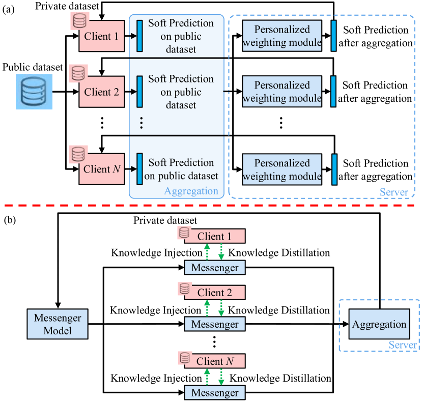
Figure 1: (a) Previous methods such as KT-pFL (Zhang et al., 2021) require an extensive public dataset to generate soft predictions to carry information from local clients to the server. These methods are highly limited by the high cost and privacy concerns of medical public datasets in real applications. (b) Our new framework MH-pFLID does not require such a public dataset for training. We use a lightweight messenger model to carry and transform the information among model heterogeneous clients and the server.

1 Introduction

Federated learning (McMahan et al., 2017) is extensively used in medical applications for its capability to train a global model collaboratively without requiring direct access to local data from each healthcare institution. Considering the local data of different healthcare institutes is mostly non-independent and identically distributed (non-IID), previous works such as (Collins et al., 2021; Deng et al., 2020; Liang et al., 2020) have focused on solving the statistic heterogeneity problems, in which the data distribution is the major difference among clients. However, system heterogeneity, such as the model architecture differences among clients, is also a commonly existing situation in real-world applications. The diverse requirements, hardware resource concerns, and regulatory risks lead different hospitals to choose and maintain different model architectures, and different model architectures result in different fitting abilities, different performance behaviors, and difficulties in model aggregation. The broad usage and problem complexity make the model heterogeneity problem a crucial and challenging task.

As illustrated in Figure 1(a), the existing methods addressing statistic and system heterogeneity are based on Knowledge Distillation (Hinton et al., 2015). These approaches involve the exchange of soft predictions on a public dataset among different clients, enabling the transfer of knowledge from one client to another (e.g., FedMD (Li & Wang, 2019), FedDF (Lin et al., 2020), KT-pFL (Zhang et al., 2021)). Although these methods have made progress in addressing system and statistic heterogeneity, they would still rely on a prerequisite public dataset to generate soft predictions. The high privacy concerns and the intricate process of collecting and publishing medical data restrict the practical applicability of these methods. Moreover, the large scale of public datasets makes local training challenging. It is uneasy for many healthcare institutions to acquire the computational resources for training on large public datasets. This could be even more burdensome considering these extra required computational resources are not needed during inference time (Baltabay et al., 2023).

To eliminate the reliance on public datasets, we propose a novel injection-distillation paradigm to address the challenges of heterogeneous models under the distribution of non-IID data. Unlike traditional approaches that rely on soft prediction generated from public datasets, our method utilizes an extremely lightweight messenger model for information transfer. Our paradigm consists of three steps: knowledge injection, knowledge distillation, and aggregation. We insert the messenger model into each local client. During the knowledge injection phase, the knowledge from the messenger is injected into each local model. During the knowledge distillation phase, the client’s knowledge is distilled into the messenger model while training on local data. In the knowledge aggregation phase, we aggregate the knowledge by combining the parameters of the messenger models. Additionally, the small parameter size of our messenger model ensures that its local training imposes minimal additional burden compared to local training on the local dataset. This additional load is less than what would be required for local training on a public dataset.

We name our framework as Model Heterogeneous personalized Federated Learning via Injection and Distillation (MH-pFLID). To facilitate efficient information transfer among heterogeneous models using a compact messenger model, we conceptualize the messenger model as a set of information bases. This approach is more efficient than directly embedding information in the messenger, while still allowing for the recovery of information acquired from local data. The messenger model comprises a codebook for storing globally shared information and a head for supervised training. In the injection phase, an attention-based, client-specific information receiver is employed for each client to receive information from the messenger. This receiver gets client-specific biases from global information, enabling the model to get other client information within the receiver and receive the generalizable information in the codebook. Similarly, during the distillation phase, a client-specific information transmitter is employed to relay information from the local model to the codebook. This disentanglement design significantly enhances the representation capacity of the messenger model and reduces biased information collected from each client, thus mitigating the issue of client drift.

In summary, our contributions include the following:

• We propose a personalized federated learning method for heterogeneous models based on an injection-distillation paradigm named MH-pFLID. Compared to previous methods, MH-pFLID eliminates reliance on public medical datasets and the associated extra costs of local training.

• We design a lightweight messenger model to transfer information among different clients. The messenger can efficiently integrate information from each client via a codebook-style design, while barely increasing local training costs.

• We design a set of transmitter and receiver modules for each client to disentangle local biases from generalizable information. This disentanglement effectively reduces the biased information gathered from each client, thereby addressing and reducing the problem of client drift.

• We validate our MH-pFLID on multiple medical tasks, including medical image classification, medical image segmentation, and medical time series classification. The experimental results show that our method outperforms state-of-the-art results on all these tasks, proving its effectiveness and generalizability in various medical applications.

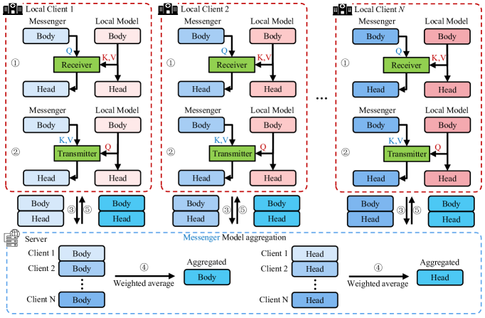
Figure 2: Overview of our proposed MH-pFLID framework. Each training cycle consists of 5 steps. From 1 to 5: ① Knowledge injection stage. We design an Information Receiver module to utilize the aggregated information in Messenger to train the local model. ② Knowledge distillation stage. We design an Information Transmitter module to transmit the personalized information from the local model to the messenger. ③ Uploading the messenger parameters on each client to the server. ④ Messenger aggregation on the server using a weighted average strategy. ⑤ Downloading the aggregated messenger parameters to each server. More details can be found in Section 3.2 and Section 3.3.

2 Related Works

2.1 Personalized Federated Learning in Statistic Heterogeneity

For classic federated learning algorithms such as the FedAvg (McMahan et al., 2017), SCAFFOLD (Karimireddy et al., 2020) and FedProx (Li et al., 2020), aiming to train a single global model across all clients. Some work has shown that when faced with statistic heterogeneity issues, it is difficult for a single model to have good performance in all clients. Personalized Federated learning is proposed to train a personalized model for each client to effectively alleviate the above problems. It includes methods such as clustering (Sattler et al., 2020; Mansour et al., 2020), model interpolation(Li et al., 2021; Deng et al., 2020; Wang et al., 2022), multi-task learning (Li et al., 2021; Mills et al., 2021; Hanzely & Richtárik, 2020; Huang et al., 2021), local memorization (Marfoq et al., 2022b) and parameter decoupling (Collins et al., 2021; Liang et al., 2020; Arivazhagan et al., 2019; Chen et al., 2020; Marfoq et al., 2022a).

2.2 Personalized Federated Learning in System Heterogeneity

In recent years, some studies used Knowledge Distillation (KD) (Hinton et al., 2015) to solve the problem of system heterogeneity. The principle is to aggregate local soft predictions in the server such as FedMD (Li & Wang, 2019) and DS-pFL (Itahara et al., 2023). To further address the issues of statistic heterogeneity and system heterogeneity, FedDF (Lin et al., 2020) adopts ensemble distillation methods to train heterogeneous models in the server. KT-pFL (Zhang et al., 2021) trains personalized soft prediction weights on the server side to further improve the performance of heterogeneous models. The above methods have made good progress in the study of system heterogeneity. However, their commonality is the need for public datasets and central computing burden. These commonalities limit the use of these methods in medical scenarios. pFedES (Yi et al., 2023b) and FedLoRA (Yi et al., 2023a) introduced additional parameters to guide local model training, alleviating some commonalities.

3 Method

3.1 Problem Formulation

We aim to train a personalized model $f_{i}(\theta_{i};x)$ for client $i$, where $\theta_{i}$ is the parameters of $f_{i}$ and $x$ is model input. Each model $f_{i}$ can only access its own private dataset $D_{i}=\{x_{ij},y_{ij}\}$, where $x_{ij}$ is the $j$th input data in $D_{i}$, and $y_{ij}$ is the $j$th label. We train all $f_{i}$ collaboratively so that each model can use the information from other clients’ datasets without directly accessing data. In real medical scenarios, the data distribution of each client is usually non-IID (statistic heterogeneity). MH-pFLID’s paradigm can be expressed as:

$$\mathbb{G}=\bigcup^{N}_{i}{f_{i}(\theta_{i};x)},$$ (1)

where $\mathbb{G}$ represents the the set of $f_{i}$. N is the total number of participating clients. Due to each client adopting a customized model architecture, the model structure $f_{i}$ of each client is different (system heterogeneity). So MH-pFLID simultaneously faces two major challenges: statistic heterogeneity and system heterogeneity across $N$ different clients.

3.2 Pipeline

The pipeline of MH-pFLID is shown in Figure 2. Both our local and messenger models are divided into a body model to extract features, and a head model to generate the network output using the features. Our training process consists of 5 steps: ① Knowledge injection, ② Knowledge distillation, ③ Uploading messenger models to the server, ④ Messenger aggregation, and ⑤ download messenger information back to the server. In the rest of the section, we will explain each step in detail.

Knowledge injection. The knowledge injection stage is designed to inject information from the messenger to the local model. Specifically, we freeze the messenger model and use the messenger model to guide the local model in training. For client $i$, its knowledge injection stage training loss function $\mathcal{L}_{\textit{inj},i}$ is:

$${\mathcal{L}_{\textit{inj},i}}=\lambda^{l}_{\textit{inj}}\sum\limits_{j=1}^{M}{\mathcal{L}^{l}_{\textit{inj}}(\hat{y}^{l}_{ij},y_{ij})}+{\lambda^{m}_{\textit{inj}}}\sum\limits_{j=1}^{M}{\mathcal{L}^{m}_{\textit{inj}}(\hat{y}^{m}_{ij},y_{ij})}.$$ (2)

$M$ represents the total number of local data. $\hat{y}^{l}_{ij}$ and $\hat{y}^{m}_{ij}$ are the predictions of the local model and messenger model for the $j$-th data of the local client. $\mathcal{L}^{l}_{\textit{inj}}$ and $\mathcal{L}^{m}_{\textit{inj}}$ represent the loss functions of the local model and the messenger model, respectively. $\lambda^{l}_{\textit{inj}}$ and $\lambda^{m}_{\textit{inj}}$ are their corresponding weights. $y_{ij}$ is the label of $x_{ij}$. Here, the local model output $\hat{y}^{l}_{ij}$ can be defined as

$$\hat{y}^{l}_{ij}=L_{h}(L_{b}(x_{ij})),$$ (3)

where $L_{b}(\cdot)$ and $L_{h}(\cdot)$ are the body and head of the local model, respectively. The messenger model output $\hat{y}^{m}_{ij}$ can be represented as

$$\hat{y}^{m}_{ij}=M_{h}(R(M_{b}(x_{ij}),L_{b}(x_{ij}))),$$ (4)

where $M_{b}(\cdot)$ is the messenger body network in Fig.2, $L_{b}(\cdot)$ is the local model body, $R(\cdot)$ is our designed receiver module to receive information from the messenger model (See Section 3.3 for details), and $M_{h}(\cdot)$ is the messenger head. During the knowledge injection stage, since the messenger model is fixed, the loss can only generate gradients on $L_{b}(\cdot)$ and $L_{h}(\cdot)$ via the first term of Equation 2, and on $L_{b}(\cdot)$ and $R(\cdot)$ via the second term of Equation 2.

Knowledge distillation. The knowledge distillation stage is designed to distill information from the local model to the messenger. Specifically, we freeze the local model and perform knowledge distillation on the messenger model, where the loss function $\mathcal{L}_{\textit{dis},i}$ is represented as:

$${\mathcal{L}_{\textit{dis},i}}=\lambda^{m}_{\textit{dis}}\sum\limits_{j=1}^{M}\mathcal{L}^{m}_{\textit{dis}}(\hat{y}^{m}_{ij},y_{ij})+{\lambda^{con}_{\textit{dis}}}\sum\limits_{j=1}^{M}{\mathcal{L}^{con}_{\textit{dis}}(\hat{y}^{m}_{ij},\hat{y}^{l}_{ij})}.$$ (5)

$\mathcal{L}^{m}_{\textit{dis}}$ and $\mathcal{L}^{con}_{\textit{dis}}$ represent the loss function for training the messenger model and the knowledge distillation loss function, respectively. For knowledge distillation loss, we use KL divergence to constrain the output of the messenger head and local head model to be under the same distribution, so that the knowledge can be distilled from the local model to the messenger model. $\lambda^{l}_{\textit{dis}}$ and $\lambda^{con}_{\textit{dis}}$ are their corresponding weights. Other variables are defined the same as in Equation 2. Here, the local model output $\hat{y}^{l}_{ij}$ is defined the same as Equation 3. The messenger model output $\hat{y}^{m}_{ij}$ can be represented as

$$\hat{y}^{m}_{ij}=M_{h}(T(L_{b}(x_{ij}),M_{b}(x_{ij}))),$$ (6)

where $M_{b}(\cdot)$, $L_{b}(\cdot)$, and $M_{h}(\cdot)$ are defined the same as in Equation 4. $T(\cdot)$ is our designed transmitter module to send information from the local model to the messenger (See Section 3.3 for details). During the training of knowledge distillation stage, we try to use both ground-truth $y_{ij}$ and local model output $\hat{y}^{l}_{ij}$ to supervised $\hat{y}^{m}_{ij}$ together, so that the knowledge can be distilled to messenger model. Since the local model is fixed, the loss generates gradients on $M_{b}(\cdot)$ $M_{h}(\cdot)$, and $T(\cdot)$ via the first and second term of Equation 5.

Messenger upload, aggregation, and download. After training, the messenger is uploaded to the server. Then aggregation of model parameters is performed separately for the body and head of the messenger. The aggregation operation used is the weight averaging from  (McMahan et al., 2017), which involves adding up all parameters and dividing them together. Finally, the aggregated model is downloaded and distributed for the next round of training.

During the inference phase, we directly utilize the well-trained local heterogeneous models for inference. Compared to other existing methods, MH-pFLID eliminates the need for a public dataset. It only inserts lightweight messenger models locally. This enhances the application of model heterogeneous federated learning in medical scenarios.

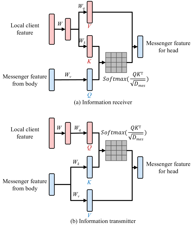
Figure 3: The structure of information receiver (a) and information transmitter (b).

3.3 Information Receiver and Information Transmitter

Information receiver and transmitter are designed to effectively communicate between local models and the messenger. To achieve a lightweight messenger model, our receiver and transmitter are designed so that the messenger would only need to carry a codebook of the information distilled from local models. The receiver module combines the information from the messenger codebook and injects it into the local model, while the transmitter module decomposes the information from local model and distills it into the messager.

Information receiver. The information receiver can be defined as $I_{\textit{loc},R}=R(I_{\textit{loc}},I_{\textit{mes}})$, where $I_{\textit{loc}}$ and $I_{\textit{mes}}$ are the output feature of local and messenger body, respectively. $I_{\textit{loc},R}$ is the output of the receiver, which is a weighted combination of local body features. In the knowledge injection stage, we design the information receiver to better match local features with global features. It can enable local models to better receive global knowledge. The information receiver, as illustrated in Figure 3(a), involves the initial generation of local client features, denoted as $I_{\textit{loc}}$, which undergoes upsampling or downsampling via a linear layer $W_{d}$ to create features $I^{\prime}_{\textit{loc}}$ with the same dimensions $D_{\textit{mes}}$ as ${I_{\textit{mes}}}$.

$$I^{\prime}_{\textit{loc}}=W_{d}({I_{\textit{loc}}}).$$ (7)

${I_{\textit{mes}}}$ and ${I^{\prime}_{\textit{loc}}}$ are used to generate Query feature $Q$, Key feature $K$ and Value feature $V$ through $W_{k}$, $W_{q}$ and $W_{v}$. The Query feature $K$ and Key feature $Q$ undergo matrix multiplication to generate the confusion matrix $M_{R}$ as:

$$\begin{array}[]{c}Q={W_{q}}({I_{\textit{mes}}}),K={W_{k}}(I^{\prime}_{\textit{loc}}),V={W_{v}}(I^{\prime}_{\textit{loc}}).\\ M_{R}=\textit{Softmax}(\frac{{Q{K^{\top}}}}{{\sqrt{{D_{\textit{mes}}}}}}).\end{array}$$ (8)

Finally, the confusion matrix $M_{R}$ is used to perform matrix multiplication with $V$, generating local features ${I_{loc,R}}$ after Information Receiver:

$${I_{\textit{loc},R}}=M_{R}{V}.$$ (9)

Information transmitter. The information transmitter can be defined as $I_{\textit{mes},T}=T(I_{\textit{mes}},I_{\textit{loc}})$, where $I_{\textit{mes},T}$ is the output of the transmitter, which is a weighted combination of messenger body features, shown in Figure 3(b). Similar to the knowledge injection stage, in the knowledge distillation stage, we allow global features ${I_{\textit{mes}}}$ to learn the knowledge of the processed local features $I^{\prime}_{\textit{loc}}$. ${I_{\textit{mes}}}$ and $I^{\prime}_{\textit{loc}}$ are used to generate Query feature $Q$, Key feature $K$ and Value feature $V$ through $W_{k}$, $W_{q}$ and $W_{v}$. The Query feature $Q$ and Key feature $K$ undergo matrix multiplication to generate the confusion matrix $M_{T}$.

$$\begin{array}[]{c}Q={W_{q}}(I^{\prime}_{\textit{loc}}),K={W_{k}}({I_{\textit{mes}}}),V={W_{v}}({I_{\textit{mes}}}).\\ M_{T}=Softmax(\frac{{Q{K^{\top}}}}{{\sqrt{{D_{\textit{mes}}}}}}).\end{array}$$ (10)

Finally, the confusion matrix $M_{T}$ is used to perform matrix multiplication with ${I_{\textit{mes}}}$, generating global features ${I_{\textit{mes},T}}$ after Information Transmitter:

$${I_{\textit{mes},T}}=M_{T}{V}.$$ (11)

At inference time, we only need the local model. The messenger model, transmitter, and receiver will not participate in inference.

Table 1: The results of classification task in different resolutions. The x2↓, x4↓, and x8↓ are downsampling half, quarter, and eighth of high-resolution images. We evaluate ACC and MF1 result on BreaKHis dataset. The larger the better. Bold number means the best. The red and green boxes respectively represent the single model federated learning and personalized federated learning methods, and their individual clients use the unified model settings (ResNet17). The blue boxes represent the method of using heterogeneous models. The four client models are set to ResNet$\{17,11,8,5\}$, respectively. MH-pFLID achieves the best performance.

Method	high-resolution		x2↓		x4↓		x8↓		Average
	ACC$\uparrow$	MF1$\uparrow$	ACC$\uparrow$	MF1$\uparrow$	ACC$\uparrow$	MF1$\uparrow$	ACC$\uparrow$	MF1$\uparrow$	ACC$\uparrow$	MF1$\uparrow$
Only Local Training	0.7891	0.7319	0.8027	0.7461	0.7538	0.6852	0.6956	0.5867	0.7603	0.6875
FedAvg	0.7406	0.6425	0.7908	0.7405	0.6892	0.6031	0.5774	0.4681	0.6995	0.6136
FedAvg+FT	0.7749	0.7218	0.8124	0.7511	0.7327	0.6628	0.6234	0.5073	0.7359	0.6608
SCAFFOLD	0.7442	0.6512	0.8097	0.7533	0.6725	0.5963	0.5866	0.4732	0.7033	0.6185
SCAFFOLD+FT	0.7761	0.7229	0.8237	0.7709	0.7523	0.6872	0.6142	0.5005	0.7416	0.6704
FedProx	0.7354	0.6386	0.7873	0.7421	0.6944	0.6107	0.5821	0.4687	0.6998	0.6150
FedProx+FT	0.7827	0.732	0.8055	0.7549	0.7548	0.6811	0.6071	0.4829	0.7375	0.6627
Ditto	0.7304	0.6221	0.7661	0.6482	0.6065	0.5022	0.5931	0.4741	0.6740	0.5617
APFL	0.7444	0.6568	0.7992	0.7355	0.6227	0.5229	0.6133	0.4986	0.6949	0.6035
FedRep	0.7991	0.7618	0.8229	0.7697	0.7762	0.7182	0.6328	0.5091	0.7578	0.6897
LG-FedAvg	0.7972	0.7523	0.5655	0.4397	0.6131	0.5080	0.6080	0.4902	0.6460	0.5476
FedMD	0.7599	0.7083	0.8321	0.7829	0.7721	0.6893	0.6495	0.5439	0.7534	0.6811
FedDF	0.7661	0.7253	0.8132	0.7629	0.7826	0.7342	0.6627	0.5627	0.7562	0.6963
pFedDF	0.8233	0.7941	0.8369	0.7965	0.8121	0.7534	0.6843	0.6022	0.7892	0.7366
DS-pFL	0.7842	0.7609	0.8334	0.7967	0.7782	0.7258	0.6327	0.5229	0.7571	0.7016
KT-pFL	0.8424	0.8133	0.8441	0.8011	0.7801	0.7325	0.7032	0.6219	0.7925	0.7422
MH-pFLID (Ours)	0.8929	0.8658	0.8992	0.8787	0.8661	0.8327	0.7751	0.7130	0.8583	0.8226

Table 2: The results of Image Classification Task with Different Label Distributions. This task includes breast cancer classification and OCT disease classification. We evaluate ACC and MF1 result in this task. The larger the better. Bold number means the best. MH-pFLID has the best performance.

Breast cancer classification
Method	ResNet		shufflenetv2		ResNeXt		squeezeNet		SENet		MobileNet		DenseNet		VGG		Average
	ACC$\uparrow$	MF1$\uparrow$	ACC$\uparrow$	MF1$\uparrow$	ACC$\uparrow$	MF1 $\uparrow$	ACC$\uparrow$	MF1$\uparrow$	ACC$\uparrow$	MF1$\uparrow$	ACC$\uparrow$	MF1$\uparrow$	ACC$\uparrow$	MF1$\uparrow$	ACC$\uparrow$	MF1$\uparrow$	ACC$\uparrow$	MF1$\uparrow$
Only Local Training	0.59	0.455	0.845	0.8412	0.665	0.5519	0.84	0.7919	0.875	0.849	0.755	0.5752	0.855	0.6884	0.875	0.8515	0.7875	0.7005
FedMD	0.692	0.5721	0.823	0.8027	0.704	0.6087	0.875	0.8544	0.907	0.8745	0.762	0.6627	0.835	0.6493	0.842	0.8001	0.8050	0.7281
FedDF	0.721	0.5949	0.817	0.8094	0.723	0.6221	0.893	0.8735	0.935	0.9021	0.757	0.6609	0.847	0.6819	0.833	0.7826	0.8158	0.7409
pFedDF	0.755	0.6536	0.853	0.8256	0.741	0.6237	0.894	0.8742	0.935	0.9021	0.796	0.7219	0.879	0.7095	0.874	0.8521	0.8409	0.7703
DS-pFL	0.715	0.6099	0.792	0.7734	0.765	0.6547	0.899	0.8792	0.935	0.9021	0.794	0.7331	0.853	0.6691	0.851	0.8266	0.8255	0.7560
KT-pFL	0.765	0.6733	0.87	0.8331	0.755	0.6432	0.885	0.8621	0.935	0.9021	0.78	0.6931	0.865	0.6819	0.905	0.9023	0.8450	0.7739
MH-pFLID (Ours)	0.820	0.6927	0.945	0.9394	0.81	0.7604	0.965	0.9457	0.982	0.9709	0.815	0.7755	0.905	0.7287	0.974	0.9583	0.9006	0.8465
OCT disease classification
Method	ResNet		shufflenetv2		ResNeXt		squeezeNet		SENet		MobileNet		DenseNet		VGG		Average
	ACC$\uparrow$	MF1$\uparrow$	ACC$\uparrow$	MF1$\uparrow$	ACC$\uparrow$	MF1$\uparrow$	ACC$\uparrow$	MF1$\uparrow$	ACC $\uparrow$	MF1$\uparrow$	ACC$\uparrow$	MF1$\uparrow$	ACC$\uparrow$	MF1$\uparrow$	ACC$\uparrow$	MF1$\uparrow$	ACC$\uparrow$	MF1$\uparrow$
Only Local Training	0.9162	0.9099	0.8922	0.8918	0.8694	0.8253	0.8472	0.8361	0.9388	0.9311	0.914	0.7236	0.9054	0.9	0.9262	0.9077	0.9012	0.8657
FedMD	0.8828	0.8349	0.8856	0.8531	0.8246	0.7822	0.8254	0.8021	0.8552	0.8321	0.9254	0.7542	0.9254	0.9119	0.9552	0.9293	0.8850	0.8375
FedDF	0.854	0.8229	0.913	0.8936	0.865	0.8241	0.8054	0.7749	0.8926	0.8733	0.9178	0.7361	0.8958	0.8831	0.963	0.9308	0.8883	0.8424
pFedDF	0.9364	0.9152	0.92	0.913	0.881	0.8327	0.863	0.8239	0.941	0.8952	0.931	0.7249	0.897	0.8829	0.961	0.9234	0.9163	0.8639
DS-pFL	0.8432	0.8079	0.864	0.8604	0.874	0.8356	0.835	0.7449	0.8874	0.8821	0.8998	0.7532	0.8592	0.8264	0.8814	0.8731	0.8680	0.8230
KT-pFL	0.9532	0.9392	0.965	0.963	0.8594	0.8466	0.9136	0.9067	0.955	0.943	0.9622	0.8099	0.9038	0.8794	0.927	0.9022	0.9299	0.8988
MH-pFLID (Ours)	0.9644	0.9516	0.992	0.983	0.898	0.8646	0.9742	0.966	0.971	0.9661	0.9544	0.8162	0.9162	0.9121	0.966	0.9511	0.9545	0.9263

4 Experiment Setup

4.1 Tasks and Datasets

We verify the effectiveness of MH-pFLID on 4 non-IID tasks.

A. Medical image classification (different resolution). We use the Breast Cancer Histopathological Image Database (BreaKHis) (Spanhol et al., 2016). We perform x2↓, x4↓, and x8↓ downsampling on the high-resolution images (Spanhol et al., 2016). Each resolution of medical images is treated as a client, resulting in four clients in total. The dataset for each client was randomly divided into training and testing sets at a ratio of 7:3, following previous work. For the same image with different resolutions, they will be used in either the training set or the testing set. In this task, we employed ResNet$\{17,11,8,5\}$.

B. Medical image classification (different label distributions). This task includes a breast cancer classification task and an OCT disease classification task. We design eight clients, each corresponding to a distinct heterogeneous model. These models include ResNet (He et al., 2015), ShuffleNetV2 (Ma et al., 2018), ResNeXt (Xie et al., 2017), SqueezeNet (Iandola et al., 2016), SENet (Hu et al., 2018), MobileNetV2 (Sandler et al., 2018), DenseNet (Huang et al., 2017), and VGG (Simonyan & Zisserman, 2014). Similar to FedAvg, we apply non-IID label distribution methods to BreaKHis (RGB images) and OCT2017 (grayscale images) (Kermany et al., 2018) across 8 clients.Specifically, in different clients, the label of each client is set to be different. Besides, the data distribution is also different among clients.

C. Medical time-series classification. We used the Sleep-EDF dataset (Goldberger et al., 2000) for the classification task of time series under non-IID distribution. We designed three clients using the TCN (Bai et al., 2018), Transformer (Zerveas et al., 2021) and RNN (Xie et al., 2024).

D. Medical image segmentation. Here, we focus on polyp segmentation (Dong et al., 2021). The dataset consists of endoscopic images collected and annotated from four centers, with each center’s dataset treats as a separate client. Each client utilized a specific model, including Unet++ (Zhou et al., 2019), FCN (Long et al., 2015), Unet (Ronneberger et al., 2015), and Res-Unet (Diakogiannis et al., 2020).

4.2 Implementation Details

MH-pFLID adopts learning rate of 0.0001 and 0.00001 for the knowledge injection and knowledge distillation stage. The batch size is set to 8. In experiments, all frameworks have a communication round of 100. Local training epochs are 5 (4 epochs in the first stage and 1 round in the second stage for MH-pFLID). For classification, $\mathcal{L}^{l}_{\textit{inj}}$, $\mathcal{L}^{m}_{\textit{inj}}$ and $\mathcal{L}^{m}_{\textit{dis}}$ are cross-entropy loss. $\mathcal{L}^{con}_{\textit{dis}}$ is KL loss (Aggarwal et al., 2021). And for segmentation tasks, $\mathcal{L}^{l}_{\textit{inj}}$, $\mathcal{L}^{m}_{\textit{inj}}$ and $\mathcal{L}^{m}_{\textit{dis}}$ are Dice loss. $\mathcal{L}^{con}_{\textit{dis}}$ still is KL loss. $\lambda^{l}_{\textit{inj}}$ and $\lambda^{l}_{\textit{dis}}$ are set to 0.9. $\lambda^{m}_{\textit{inj}}$ and $\lambda^{con}_{\textit{dis}}$ are 0.1.The performance evaluation of the classification task is based on two metrics, accuracy (ACC) and macro-averaged F1-score (MF1), providing a comprehensive assessment of the model’s robustness. Additionally, Dice is used to evaluate the segmentation task performance across frameworks.

Table 3: The results of the time-series classification task. MH-pFLID performs the best. We evaluate ACC and MF1 result in this task. The larger the better. Bold number means the best. MH-pFLID has the best performance.

Method	TCN		Transformer		RNN		Average
	ACC$\uparrow$	MF1$\uparrow$	ACC$\uparrow$	MF1$\uparrow$	ACC$\uparrow$	MF1$\uparrow$	ACC$\uparrow$	MF1$\uparrow$
Only Local Training	0.9073	0.8757	0.8053	0.8001	0.8012	0.7263	0.8379	0.8007
FedMD	0.9334	0.9225	0.7934	0.7966	0.793	0.7072	0.8399	0.8088
FedDF	0.9146	0.8893	0.7988	0.8042	0.7881	0.6855	0.8338	0.7930
pFedDF	0.9173	0.8957	0.827	0.8309	0.8137	0.7713	0.8527	0.8326
DS-pFL	0.9133	0.9033	0.8253	0.8301	0.8042	0.7539	0.8476	0.8291
KT-pFL	0.9240	0.9089	0.8419	0.8466	0.8204	0.7722	0.8621	0.8426
MH-pFLID (Ours)	0.9439	0.9248	0.8725	0.876	0.824	0.7773	0.8801	0.8594

Table 4: For the medical image segmentation task, we evaluate the Dice result on Polyp dataset. The larger the better. Bold number means the best. The red and green boxes represent the single model federated learning and personalized federated learning methods, respectively. Their individual clients use the unified model settings (Unet). The blue boxes represent the method of using heterogeneous models in each client. The four client models are set to Unet++, FCN, Unet, and ResUnet, respectively. MH-pFLID achieves the best segmentation results.

Methods	Client1	Client2	Client3	Client4	Average
FedAvg	0.5249	0.4205	0.5676	0.5500	0.5158
FedAvg+FT	0.6047	0.4762	0.7513	0.6681	0.6251
SCAFFOLD	0.5244	0.3591	0.5935	0.5713	0.5121
SCAFFOLD+FT	0.5937	0.4312	0.8231	0.7208	0.6422
FedProx	0.5529	0.4674	0.5403	0.6301	0.5477
FedProx+FT	0.7441	0.5701	0.7438	0.6402	0.6746
Ditto	0.5720	0.4644	0.6648	0.6416	0.5857
APFL	0.6120	0.5095	0.6333	0.5892	0.5860
LG-FedAvg	0.6053	0.5062	0.7371	0.5596	0.6021
FedRep	0.5809	0.3106	0.7088	0.7023	0.5757
FedSM	0.6894	0.6278	0.8021	0.7391	0.7146
LC-Fed	0.6233	0.4982	0.8217	0.7654	0.6772
Only Local Training	0.7049	0.4906	0.8079	0.7555	0.6897
MH-pFLID (Ours)	0.7591	0.6528	0.8543	0.7752	0.7604

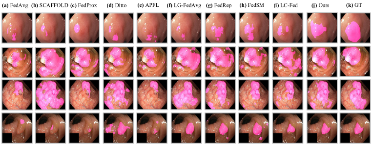
Figure 4: Visualized comparison of Federated Learning in medical image segmentation. We randomly select four samples from different clients to form the visualization. (a-j) Segmentation results by a model trained with FedAVG, SCAFFOLD, FedProx, Ditto, APFL, LG-FedAvg, FedRep, FedSM, LC-Fed, and our method MH-pFLID; (k) Ground truths (denoted as ‘GT’).

Table 5: GFLOPS and parameters of local heterogeneous models and messenger models in various tasks. The smaller the better. Bold number means the best. Among the four tasks, the GFLOPS and parameters of the messenger models are much smaller than those of the local models.

Tasks	Dataset	Model	GFLOPS	#Params
Medical Image Classification (Different Resolution)	BreaKHis (384x384x3 - 48x48x3)	ResNet17	3.495	4.231M
		ResNet11	0.667	2.104M
		ResNet8	0.140	1.558M
		ResNet5	0.044	1.359M
		Messeger	0.01-0.07	0.035M
Medical Image Classification (Different Label Distributions)	BreaKHis (384x384x3)	ResNet	10.020	11.111M
		Shufflenetv2	1.719	1.730M
		ResNeXt	41.245	7.930M
		squeezeNet	7.774	1.832M
		SENet	80.370	12.372M
		MobileNet	1.870	1.934M
		DenseNet	13.461	1.147M
		VGG	57.524	40.045M
		Messeger	0.070	0.032M
	OCT 2017 (256x256x1)	ResNet	4.351	11.090M
		Shufflenetv2	0.735	1.712M
		ResNeXt	18.256	7.910M
		squeezeNet	3.342	1.820M
		SENet	35.644	12.363M
		MobileNet	0.812	1.921M
		DenseNet	5.954	1.14M
		VGG	25.501	40.020M
		Messeger	0.012	0.035M
Medical Time-series Classification Task	Sleep-EDF (1x3000)	TCN	17.101	1.182M
		Transformer	1.224	1.134M
		RNN	5.200	1.236M
		Messeger	0.411	0.003M
Medical Image Segmentation Task	Polyp (256x256x3)	Unet++	34.906	10.421M
		FCN	54.742	32.560M
		Unet	56.435	33.090M
		ResUnet	25.572	19.913M
		Messeger	0.681	0.196M

5 Results

5.1 Medical Image Classification (Different Resolutions)

In this task, we employ models from the ResNet family to train breast cancer medical images at different resolutions. For low-resolution images, we use shallow ResNet models for training, while for high-resolution images, we employ deeper and more complex ResNet models. In Table 1, compared to other federated learning frameworks, MH-pFLID achieves the best performance on all clients of different resolutions, including the original high-resolution, half(“$\times 2\downarrow$”), quarter (“$\times 4\downarrow$”), and one eighth (“$\times 8\downarrow$”). This indicates that MH-pFLID, based on the injection and distillation paradigm, effectively enables local heterogeneous models within the same family to learn global knowledge, thereby enhancing the performance of local models. Furthermore, MH-pFLID demonstrates a more significant advantage in terms of the MF1 metric, highlighting its ability to improve the robustness of local heterogeneous models.

5.2 Medical Image Classification (Different Label Distributions)

In Table 2, the experimental results for the medical image classification task with different label distributions, where each client uses heterogeneous models, show that MH-pFLID achieves the optimal results. This demonstrates that, compared to heterogeneous federated learning methods based on soft predictions, the Injection and Distillation approach of MH-pFLID has advantages. It can more effectively utilize knowledge from other clients to guide local client learning. Compared to local training alone, MH-pFLID enhances the local performance of each heterogeneous model. This indicates that our proposed feature adaptation method, aligning global and local features, effectively alleviates the issue of client shift when guiding client training for each heterogeneous model.

5.3 Time-series Classification

The experimental results in Table 3 show that MH-pFLID achieves the best results under different types of neural networks. This further demonstrates the superiority of MH-pFLID in federated learning of heterogeneous models.

5.4 Medical Image Segmentation

We have once again validated the effectiveness of MH-pFLID in medical image segmentation tasks. Table 4 presents the results of federated learning in the segmentation task, demonstrating that MH-pFLID achieves the best experimental outcomes. This indicates MH-pFLID applicability across multiple tasks. The experimental results further highlight that MH-pFLID effectively enhances the local model performance for each client in various tasks, surpassing existing personalized approaches for homogeneous models. Meanwhile, the visualization results in Figure 4 show that the segmentation results of MH-pFLID are closer to ground truth.

5.5 GFLOPS and Parameters

We compare the GFLOPS and parameter of the messenger model with local heterogeneous models in four tasks. The results of Table 5 show that the GFLOPS and parameters of the messenger model are much smaller than those of the local heterogeneous model.

Table 6: The ablation experiments of MH-pFLID. We remove some essential modules to verify the effectiveness of each module. We perform experiments on breast cancer classification (different label distributions) and medical image segmentation tasks. We observe that though those experiments outperform only local training, they suffer different levels of performance decrease.

Methods	Breast Cancer		Segmentation
	ACC$\uparrow$	MF1$\uparrow$	Dice$\uparrow$
MH-pFLID	0.9006	0.8465	0.7604
w/o Messenger Head	0.8657	0.7921	0.7391
w/o Messenger Body	0.8432	0.7709	0.7294
w/o Information Receiver	0.8631	0.8021	0.7339
w/o Information Transmitter	0.8791	0.8249	0.7405
w/o Information Receiver & Transmitter	0.8479	0.7853	0.7306
Only Local Training	0.7875	0.7005	0.6897

5.6 Ablation Studies

To verify the effectiveness of the proposed components in MH-pFLID, a comparison between MH-pFLID and its four components on breast cancer classification in different label distributions and segmentation tasks is given in Table 6. The four components are as follows: (1) w/o messenger head and w/o messenger body: the distilled head or body does not participate in the global aggregation stage. (2) w/o information receiver or information transmitter indicates that the information receiver or information transmitter (IT) are replaced with the feature add operation. The experimental results indicate that more parameter sharing is beneficial for MH-pFLID. information receiver and information transmitter operations effectively improve the performance of local heterogeneous models.

Table 7: Generalizability experiments of the messenger model. Our method increases the performance not only on the models’ own clients, but on other untrained clients.

	Only Local Training						Ours						Improvement
	Client1	Client2	Client3	Client4			Client1	Client2	Client3	Client4			Client1	Client2	Client3	Client4
Unet++	0.7049	0.0586	0.3016	0.2239		Unet++	0.7591	0.1596	0.3542	0.4497		Unet++	+7.1%	+63.3%	+14.9%	+50.2%
Unet	0.1393	0.4906	0.2231	0.404		Unet	0.1418	0.6528	0.225	0.4654		Unet	+0.3%	+16.2%	+0.2%	+6.1%
ResUnet	0.2433	0.1241	0.8079	0.4527		ResUnet	0.3239	0.2929	0.8543	0.6066		ResUnet	+8.1%	+16.9%	+4.6%	+15.4%
FCN	0.442	0.3247	0.4597	0.7555		FCN	0.3403	0.434	0.4855	0.7752		FCN	-10.2%	+10.9%	+2.6%	+2.0%

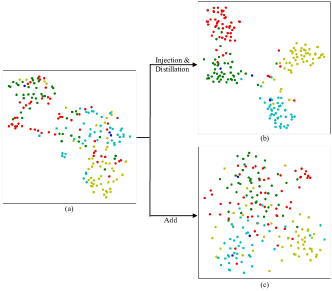
Figure 5: t-SNE map of the 7th client (DenseNet) through injection & distillation or add under breast cancer classification task (different label distributions). Different colored dots represent different categories. (a-c) are the t-SNE map of (a) the features extracted from the local model body, (b) local model body features after injection & distillation, and (c) the same feature by replacing the injection & distillation process with a simple add operation and retrained. The experimental results show that the features generated by injection & distillation are more distinguishable compared to the straightforward add design.

5.7 Feature Distribution t-SNE of Injection & Distillation Operations

We train the local heterogeneous model for 20 epochs without any other operations (The feature distribution is shown in Figure 5(a)). Next, we will perform 5 communication rounds of injection-distillation or add on the trained local heterogeneous model. The experimental results show that the injection-distillation operation (Figure 5(b)) generates more discriminative features compared to the add operation (Figure 5(c)). This is more conducive to subsequent tasks.

5.8 Generalizability Experiments of the Messenger Model

We evaluate local models directly on other clients without training on those clients’ data on the segmentation task in Table 7. We see performance increases not only on the models’ own clients, but on other untrained clients. These results verify that our messenger would increase the generalizability of the local model, thus it successfully collects generalized information from other clients.

5.9 The Disentanglement of the Bases from the Messenger

To evaluate the disentanglement, we calculate how orthogonal are those bases by calculating $e=\|BB^{\top}-I\|_{f}$ as the training proceeds, where $B$ is the bases matrix, $I$ is the identity matrix, and $\|\cdot\|_{f}$ is the Frobenius norm. If they are fully orthogonal to each other, $\|BB^{\top}-I\|_{f}$ should be equal to 0. Our experiment in the following Table 8 shows that, as the training proceeds, $e$ clearly drops, meaning our transmitter and receiver give good disentanglements.

Table 8: The disentanglement of feature bases changes in training process.

Rounds	$e=\|BB^{\top}-I\|_{f}$
1	0.44
5	0.37
10	0.11
20	0.10

6 Limitations and Conclusion

Our method has demonstrated its effectiveness in medical classification and segmentation tasks, yet we have not validated and refined our approach in medical object detection, image registration, medical 3D reconstruction, etc.. In future work, the potential of our method in these areas awaits further verification and enhancement. MH-pFLID effectively addresses challenges faced by existing personalized federated learning approaches for heterogeneous models. These challenges include collecting and labeling public datasets, and computational burden on local clients and servers. MH-pFLID, based on injection and distillation paradigm, offers a solution to these issues. MH-pFLID introduces a lightweight messenger model in each client and designs information receiver and transmitter. These can enable local heterogeneous models to transfer information from other clients well under non-IID distribution. Extensive experiments demonstrate superiority of MH-pFLID over existing frameworks for federated learning with heterogeneous models.

Impact Statements

This paper presents work whose goal is to advance the field of Machine Learning. There are many potential societal consequences of our work, none which we feel must be specifically highlighted here.

Appendix A Related Works Supplement

In this section, we provide a detailed supplement to the comparison of personalized federated learning in this paper.

APFL (Deng et al., 2020) adopts the joint prediction mode which is a mixture of global model and local model with adaptive weight. LG-FedAvg (Liang et al., 2020) and FedRep (Collins et al., 2021) use parameter decoupling to jointly learn the global part and local part of the client model, while only the global part was sent to the server. The difference between them is the definition of which part of the model is the global part. kNN-Per (Marfoq et al., 2022a) uses the output of the K global representations closest to the global representation of the input to be evaluated to make predictions. Ditto (Li et al., 2021) adds a regular term to the original local loss function of each client to measure the deviation between the local model and the global model.

Appendix B Baselines

In the medical image classification task (different resolution), we selected FedAvg, SCAFFOLD, FedProx, and their fine-tuned methods (Collins et al., 2022) same as previous work (Collins et al., 2021). Among the personalized Federated Learning methods, we compared FedRep, LG-FedAvg, APFL, and Ditto. For heterogeneous model federated learning, we chose FedMD, FedDF, pFedDF, DS-pFL, and KT-pFL.

In the medical image classification task (different label distrbutions), we compared various methods, including local training of clients with heterogeneous models and existing heterogeneous model federated learning approaches (FedMD, FedDF, pFedDF, DS-pFL, and KT-pFL).

The baseline used in the medical time-series classification task is the same as the medical image classification task (different label distrbutions).

For image segmentation tasks, we compared various approaches, including local training of clients and a variety of personalized federated learning techniques, as well as methods for learning a single global model and their fine-tuned versions. Among the personalized methods, we also chose FedRep, LG-FedAvg, APFL, and Ditto. We simultaneously added LC-Fed (Wang et al., 2022) and FedSM (Xu et al., 2022) which are effective improvements for FedRep and APFL in the federated segmentation domain.

Appendix C Datasets

A. Medical image classification (different resolution). We used the Breast Cancer Histopathological Image Database (BreaKHis) (Spanhol et al., 2016). We treat the original image as a high-resolution image. Then, the Bicubic downsampling method is used to downsample the high-resolution image, obtaining images with resolutions of x2 ↓, x4 ↓, and x8 ↓, respectively. Each resolution of medical images was treated as a separate client, resulting in four clients in total. Each client has the same number of images with consistent label distribution, but the image resolution is different for each client. The dataset for each client was randomly divided into training and testing sets at a ratio of 7:3, following previous work. In this task, we employed a family of models such as ResNet$\{17,11,8,5\}$.

B. Medical image classification (different label distributions). This task includes a breast cancer classification task and an OCT disease classification task. We designed eight clients, each corresponding to a distinct heterogeneous model. These models included ResNet (He et al., 2015), ShuffleNetV2 (Ma et al., 2018), ResNeXt (Xie et al., 2017), SqueezeNet (Iandola et al., 2016), SENet (Hu et al., 2018), MobileNetV2 (Sandler et al., 2018), DenseNet (Huang et al., 2017), and VGG (Simonyan & Zisserman, 2014). Similar to the previous approach, we applied non-IID label distribution methods to the OCT2017 (grayscale images) (Kermany et al., 2018) and BreaKHis (RGB images) across the 8 clients.

For the breast cancer classification task, we have filled in the data quantity to 8000 and allocated 1000 pieces of data to each client. The ratio of training set to testing set for each client is 8:2.

For the OCT disease classification task, we randomly selected 40000 pieces of data, with 5000 pieces per client. The ratio of training set to test set is also 8:2.

C. Medical time-series classification. We used the Sleep-EDF dataset (Goldberger et al., 2000) for the classification task of time series under Non-IID distribution. We divided the Sleep-EDF dataset evenly among three clients. The ratio of training set to testing set for each client is 8:2. We designed three clients using the TCN (Bai et al., 2018), Transformer (Zerveas et al., 2021) and RNN (Xie et al., 2024).

D. Medical image segmentation. Here, we focus on polyp segmentation (Dong et al., 2021). The dataset for this task consisted of endoscopic images collected and annotated from four different centers, with each center’s dataset treated as a separate client. Thus, there were four clients in total for this task. The number of each client are 1000, 380, 196 and 612. The ratio of training set to testing set for each client is 1:1. Each client utilized a specific model, including Unet++ (Zhou et al., 2019), FCN (Long et al., 2015), Unet (Ronneberger et al., 2015), and Res-Unet (Diakogiannis et al., 2020).

Appendix D Training Settings

D.1 Evaluation Indicators

The performance evaluation of the classification task is based on two metrics, accuracy (ACC) and macro-averaged F1-score (MF1), providing a comprehensive assessment of the model’s robustness. Additionally, Dice is used to evaluate the segmentation task performance across frameworks.

A. Accuracy. Accuracy is the ratio of the number of correct judgments to the total number of judgments.

B. Macro-averaged F1-score. First, calculate the F1-score for each recognition category, and then calculate the overall average value.

C. Dice. It is a set similarity metric commonly used to calculate the similarity between two samples, with a threshold of [0,1]. In medical images, it is often used for image segmentation, with the best segmentation result being 1 and the worst result being 0. The Dice coefficient calculation formula is as follows:

$$Dice=\frac{{2*(pred\cap true)}}{{pred\cup true}}$$ (12)

Among them, $pred$ is the set of predicted values, $true$ is the set of groudtruth values. And the numerator is the intersection between $pred$ and $true$. Multiplying by 2 is due to the repeated calculation of common elements between $pred$ and $true$ in the denominator. The denominator is the union of $pred$ and $true$.

D.2 Loss Function

Many loss functions have been applied in this article, and here are some explanations for them.The cross entropy loss function is very common and will not be explained in detail here. We mainly explain Dice loss.

Dice Loss applied in the field of image segmentation. It is represented as:

$$DiceLoss=1-\frac{{2*(pred\cap true)}}{{pred\cup true}}$$ (13)

The Dice loss and Dice coefficient are the same thing, and their relationship is:

$$DiceLoss=1-Dice$$ (14)

In knowledge distillation, we use KL divergence loss to optimize the distribution difference between the messenger model and the local model. We try to constrain the output of the messenger head and local head model to be under the same distribution, so that the knowledge can be distillated from the local model to the messenger model. The KL loss is defined as:

$$KLLoss=\sum_{i=0}^{m}[y_{i}log(y_{i})-\hat{y_{i}}log(\hat{y_{i}})]$$ (15)

where $m$ represents the total number of client data. $\hat{y_{i}}$ and $y_{i}$ represent the outputs of the messenger model and the local model, respectively.

D.3 Public Datasets for other Federated Learning of Heterogeneous Models

In this section, we mainly describe the setting of public datasets for methods such as FedMD, FedDF, DS-pFL and KT-pFL.

A. Medical image classification (different resolution). We select 100 pieces of data from each client and put them into the central server as public data, totaling 400 pieces of data as public data. In order to better obtain soft predictions for individual clients, the image resolution of the publicly available dataset will be resized to the corresponding resolution for each client.

B. Medical image classification (different label distributions). For the breast cancer classification task, we select 50 pieces of data for each client to upload, and the public dataset contains 400 images. For the OCT disease classification task, We selected 1000 pieces of data from both the non training and testing sets.

C. Medical time-series classification. We select 200 pieces of data for each client to upload, and the public dataset contains 600 images.

Appendix E The Messenger Models

For medical image classification, the structure of the messenger model is shown in Table 1.

Table 9: The structure of the messenger model in the medical image classification. In the messenger body, the stride of each layer is 2. Class represents the category.

	Layer	Operation
Messenger Body	Conv2d 3x3-64	ReLU
	MaxPool 3x3	-
	Conv2d 5x5-64	ReLU
	MaxPool 3x3	-
	Conv2d 7x7-512	ReLU
Messenger Head	Linear-256	BatchNorm1d+ReLU
	Linear-class	-

For medical image segmentation, the structure of the messenger model is shown in Table 2.

Table 10: The structure of the messenger model in the medical image segmentation. In the messenger body, the stride of each conv2d layer is 1 and MaxPool is 2. In the messenger head, the stride of each layer is 2. Class represents the category.

	Layer	Operation
Messenger Body	Conv2d 3x3-64	ReLU
	MaxPool 3x3	-
	Conv2d 5x5-64	ReLU
	MaxPool 3x3	-
	Conv2d 7x7-64	ReLU
	MaxPool 3x3	-
	Conv2d 7x7-512	ReLU
	MaxPool 3x3	-
Messenger Head	ConvTranspose2d 2x2-64	ReLU
	ConvTranspose2d 2x2-64	ReLU
	ConvTranspose2d 2x2-64	ReLU
	ConvTranspose2d 2x2-class	-

Appendix F Future Works

Our method has demonstrated its effectiveness in medical classification and segmentation tasks (Greenspan et al., 2023; Xie et al., 2024, 2022b, 2022a; Gong et al., 2021). In the future, We will extend our approach to areas such as medical object detection, image super-resolution (Xie et al., 2023), 3D reconstruction (Luan et al., 2023, 2021; Zhai et al., 2023; Luan et al., 2024; Wu et al., 2024; Gong et al., 2023), medical image generation (Chen et al., 2024), Magnetic Resonance Imaging (Chen et al., 2014), etc.. Moreover, we will also leverage the foundation models (Moor et al., 2023) into our FL framework to achieve higher performance.

References

- Aggarwal et al. (2021) Aggarwal, A., Mittal, M., and Battineni, G. Generative adversarial network: An overview of theory and applications. International Journal of Information Management Data Insights, 1(1):100004, 2021.
- Arivazhagan et al. (2019) Arivazhagan, M. G., Aggarwal, V., Singh, A. K., and Choudhary, S. Federated learning with personalization layers. arXiv preprint arXiv:1912.00818, 2019.
- Bai et al. (2018) Bai, S., Kolter, J. Z., and Koltun, V. An empirical evaluation of generic convolutional and recurrent networks for sequence modeling. arXiv preprint arXiv:1803.01271, 2018.
- Baltabay et al. (2023) Baltabay, M., Yazici, A., Sterling, M., and Ever, E. Designing efficient and lightweight deep learning models for healthcare analysis. Neural Processing Letters, pp. 1–31, 2023.
- Chen et al. (2014) Chen, X., Salerno, M., Yang, Y., and Epstein, F. H. Motion-compensated compressed sensing for dynamic contrast-enhanced mri using regional spatiotemporal sparsity and region tracking: Block low-rank sparsity with motion-guidance (blosm). Magnetic resonance in medicine, 72(4):1028–1038, 2014.
- Chen et al. (2024) Chen, X., Zhang, S., Chen, E. Z., Liu, Y., Zhao, L., Chen, T., and Sun, S. Federated data model. arXiv preprint arXiv:2403.08887, 2024.
- Chen et al. (2020) Chen, Y., Qin, X., Wang, J., Yu, C., and Gao, W. Fedhealth: A federated transfer learning framework for wearable healthcare. IEEE Intelligent Systems, 35(4):83–93, 2020.
- Collins et al. (2021) Collins, L., Hassani, H., Mokhtari, A., and Shakkottai, S. Exploiting shared representations for personalized federated learning. In ICML, pp. 2089–2099. PMLR, 2021.
- Collins et al. (2022) Collins, L., Hassani, H., Mokhtari, A., and Shakkottai, S. Fedavg with fine tuning: Local updates lead to representation learning. In Koyejo, S., Mohamed, S., Agarwal, A., Belgrave, D., Cho, K., and Oh, A. (eds.), Advances in Neural Information Processing Systems, volume 35, pp. 10572–10586. Curran Associates, Inc., 2022.
- Deng et al. (2020) Deng, Y., Kamani, M. M., and Mahdavi, M. Adaptive personalized federated learning. arXiv preprint arXiv:2003.13461, 2020.
- Diakogiannis et al. (2020) Diakogiannis, F. I., Waldner, F., Caccetta, P., and Wu, C. Resunet-a: A deep learning framework for semantic segmentation of remotely sensed data. ISPRS Journal of Photogrammetry and Remote Sensing, 162:94–114, 2020.
- Dong et al. (2021) Dong, B., Wang, W., Fan, D.-P., Li, J., Fu, H., and Shao, L. Polyp-pvt: Polyp segmentation with pyramid vision transformers. arXiv preprint arXiv:2108.06932, 2021.
- Goldberger et al. (2000) Goldberger, A. L., Amaral, L. A., Glass, L., Hausdorff, J. M., Ivanov, P. C., Mark, R. G., Mietus, J. E., Moody, G. B., Peng, C.-K., and Stanley, H. E. Physiobank, physiotoolkit, and physionet: components of a new research resource for complex physiologic signals. circulation, 101(23):e215–e220, 2000.
- Gong et al. (2021) Gong, X., Xia, X., Zhu, W., Zhang, B., Doermann, D., and Zhuo, L. Deformable gabor feature networks for biomedical image classification. In Proceedings of the IEEE/CVF Winter Conference on applications of computer vision, pp. 4004–4012, 2021.
- Gong et al. (2023) Gong, X., Song, L., Zheng, M., Planche, B., Chen, T., Yuan, J., Doermann, D., and Wu, Z. Progressive multi-view human mesh recovery with self-supervision. In Proceedings of the AAAI Conference on Artificial Intelligence, volume 37, pp. 676–684, 2023.
- Greenspan et al. (2023) Greenspan, H., Madabhushi, A., Mousavi, P., Salcudean, S., Duncan, J., Syeda-Mahmood, T., and Taylor, R. Medical Image Computing and Computer Assisted Intervention–MICCAI 2023: 26th International Conference, Vancouver, BC, Canada, October 8–12, 2023, Proceedings, Part V, volume 14224. Springer Nature, 2023.
- Hanzely & Richtárik (2020) Hanzely, F. and Richtárik, P. Federated learning of a mixture of global and local models. arXiv preprint arXiv:2002.05516, 2020.
- He et al. (2015) He, K., Zhang, X., Ren, S., and Sun, J. Deep residual learning for image recognition, 2015.
- Hinton et al. (2015) Hinton, G., Vinyals, O., and Dean, J. Distilling the knowledge in a neural network, 2015.
- Hu et al. (2018) Hu, J., Shen, L., and Sun, G. Squeeze-and-excitation networks. In Proceedings of the IEEE conference on computer vision and pattern recognition, pp. 7132–7141, 2018.
- Huang et al. (2017) Huang, G., Liu, Z., Van Der Maaten, L., and Weinberger, K. Q. Densely connected convolutional networks. In Proceedings of the IEEE conference on computer vision and pattern recognition, pp. 4700–4708, 2017.
- Huang et al. (2021) Huang, Y., Chu, L., Zhou, Z., Wang, L., Liu, J., Pei, J., and Zhang, Y. Personalized cross-silo federated learning on non-iid data. In AAAI, volume 35, pp. 7865–7873, 2021.
- Iandola et al. (2016) Iandola, F. N., Han, S., Moskewicz, M. W., Ashraf, K., Dally, W. J., and Keutzer, K. Squeezenet: Alexnet-level accuracy with 50x fewer parameters and¡ 0.5 mb model size. arXiv preprint arXiv:1602.07360, 2016.
- Itahara et al. (2023) Itahara, S., Nishio, T., Koda, Y., Morikura, M., and Yamamoto, K. Distillation-based semi-supervised federated learning for communication-efficient collaborative training with non-iid private data. IEEE Transactions on Mobile Computing, 22(1):191–205, 2023. doi: 10.1109/TMC.2021.3070013.
- Karimireddy et al. (2020) Karimireddy, S. P., Kale, S., Mohri, M., Reddi, S., Stich, S., and Suresh, A. T. Scaffold: Stochastic controlled averaging for federated learning. In ICML, pp. 5132–5143. PMLR, 2020.
- Kermany et al. (2018) Kermany, D. S., Goldbaum, M., Cai, W., Valentim, C. C., Liang, H., Baxter, S. L., McKeown, A., Yang, G., Wu, X., Yan, F., et al. Identifying medical diagnoses and treatable diseases by image-based deep learning. cell, 172(5):1122–1131, 2018.
- Li & Wang (2019) Li, D. and Wang, J. Fedmd: Heterogenous federated learning via model distillation. CoRR, abs/1910.03581, 2019.
- Li et al. (2020) Li, T., Sahu, A. K., Zaheer, M., Sanjabi, M., Talwalkar, A., and Smith, V. Federated optimization in heterogeneous networks. Proceedings of Machine learning and systems, 2:429–450, 2020.
- Li et al. (2021) Li, T., Hu, S., Beirami, A., and Smith, V. Ditto: Fair and robust federated learning through personalization. In ICML, pp. 6357–6368. PMLR, 2021.
- Liang et al. (2020) Liang, P. P., Liu, T., Ziyin, L., Allen, N. B., Auerbach, R. P., Brent, D., Salakhutdinov, R., and Morency, L.-P. Think locally, act globally: Federated learning with local and global representations. arXiv preprint arXiv:2001.01523, 2020.
- Lin et al. (2020) Lin, T., Kong, L., Stich, S. U., and Jaggi, M. Ensemble distillation for robust model fusion in federated learning. In Larochelle, H., Ranzato, M., Hadsell, R., Balcan, M., and Lin, H. (eds.), Advances in Neural Information Processing Systems, volume 33, pp. 2351–2363. Curran Associates, Inc., 2020.
- Long et al. (2015) Long, J., Shelhamer, E., and Darrell, T. Fully convolutional networks for semantic segmentation. In Proceedings of the IEEE conference on computer vision and pattern recognition, pp. 3431–3440, 2015.
- Luan et al. (2021) Luan, T., Wang, Y., Zhang, J., Wang, Z., Zhou, Z., and Qiao, Y. Pc-hmr: Pose calibration for 3d human mesh recovery from 2d images/videos. In Proceedings of the AAAI Conference on Artificial Intelligence, volume 35, pp. 2269–2276, 2021.
- Luan et al. (2023) Luan, T., Zhai, Y., Meng, J., Li, Z., Chen, Z., Xu, Y., and Yuan, J. High fidelity 3d hand shape reconstruction via scalable graph frequency decomposition. In Proceedings of the IEEE/CVF Conference on Computer Vision and Pattern Recognition, pp. 16795–16804, 2023.
- Luan et al. (2024) Luan, T., Li, Z., Chen, L., Gong, X., Chen, L., Xu, Y., and Yuan, J. Spectrum auc difference (saucd): Human-aligned 3d shape evaluation. arXiv preprint arXiv:2403.01619, 2024.
- Ma et al. (2018) Ma, N., Zhang, X., Zheng, H.-T., and Sun, J. Shufflenet v2: Practical guidelines for efficient cnn architecture design. In Proceedings of the European conference on computer vision (ECCV), pp. 116–131, 2018.
- Mansour et al. (2020) Mansour, Y., Mohri, M., Ro, J., and Suresh, A. T. Three approaches for personalization with applications to federated learning. arXiv preprint arXiv:2002.10619, 2020.
- Marfoq et al. (2022a) Marfoq, O., Neglia, G., Vidal, R., and Kameni, L. Personalized federated learning through local memorization. In ICML, pp. 15070–15092. PMLR, 2022a.
- Marfoq et al. (2022b) Marfoq, O., Neglia, G., Vidal, R., and Kameni, L. Personalized federated learning through local memorization. In Chaudhuri, K., Jegelka, S., Song, L., Szepesvari, C., Niu, G., and Sabato, S. (eds.), Proceedings of the 39th International Conference on Machine Learning, volume 162 of Proceedings of Machine Learning Research, pp. 15070–15092. PMLR, 17–23 Jul 2022b.
- McMahan et al. (2017) McMahan, B., Moore, E., Ramage, D., Hampson, S., and y Arcas, B. A. Communication-efficient learning of deep networks from decentralized data. In AISTATS, pp. 1273–1282. PMLR, 2017.
- Mills et al. (2021) Mills, J., Hu, J., and Min, G. Multi-task federated learning for personalised deep neural networks in edge computing. IEEE Transactions on Parallel and Distributed Systems, 33(3):630–641, 2021.
- Moor et al. (2023) Moor, M., Banerjee, O., Abad, Z. S. H., Krumholz, H. M., Leskovec, J., Topol, E. J., and Rajpurkar, P. Foundation models for generalist medical artificial intelligence. Nature, 616(7956):259–265, 2023.
- Ronneberger et al. (2015) Ronneberger, O., Fischer, P., and Brox, T. U-net: Convolutional networks for biomedical image segmentation. In Medical Image Computing and Computer-Assisted Intervention–MICCAI 2015: 18th International Conference, Munich, Germany, October 5-9, 2015, Proceedings, Part III 18, pp. 234–241. Springer, 2015.
- Sandler et al. (2018) Sandler, M., Howard, A., Zhu, M., Zhmoginov, A., and Chen, L.-C. Mobilenetv2: Inverted residuals and linear bottlenecks. In Proceedings of the IEEE conference on computer vision and pattern recognition, pp. 4510–4520, 2018.
- Sattler et al. (2020) Sattler, F., Müller, K.-R., and Samek, W. Clustered federated learning: Model-agnostic distributed multitask optimization under privacy constraints. IEEE transactions on neural networks and learning systems, 32(8):3710–3722, 2020.
- Simonyan & Zisserman (2014) Simonyan, K. and Zisserman, A. Very deep convolutional networks for large-scale image recognition. arXiv preprint arXiv:1409.1556, 2014.
- Spanhol et al. (2016) Spanhol, F. A., Oliveira, L. S., Petitjean, C., and Heutte, L. A dataset for breast cancer histopathological image classification. IEEE Transactions on Biomedical Engineering, 63(7):1455–1462, 2016. doi: 10.1109/TBME.2015.2496264.
- Wang et al. (2022) Wang, J., Jin, Y., and Wang, L. Personalizing federated medical image segmentation via local calibration. In ECCV, pp. 456–472. Springer, 2022.
- Wu et al. (2024) Wu, X., Wu, X., Luan, T., Bai, Y., Lai, Z., and Yuan, J. Fsc: Few-point shape completion. arXiv preprint arXiv:2403.07359, 2024.
- Xie et al. (2022a) Xie, L., Shen, Y., Zhang, M., Zhong, Y., Lu, Y., Yang, L., and Li, Z. Single-model multi-tasks deep learning network for recognition and quantitation of surface-enhanced raman spectroscopy. Optics Express, 30(23):41580–41589, 2022a.
- Xie et al. (2022b) Xie, L., Zhong, Y., Yang, L., Yan, Z., Wu, Z., and Wang, J. Tc-sknet with gridmask for low-complexity classification of acoustic scene. In 2022 Asia-Pacific Signal and Information Processing Association Annual Summit and Conference (APSIPA ASC), pp. 1091–1095. IEEE, 2022b.
- Xie et al. (2023) Xie, L., Li, C., Wang, Z., Zhang, X., Chen, B., Shen, Q., and Wu, Z. Shisrcnet: Super-resolution and classification network for low-resolution breast cancer histopathology image, 2023.
- Xie et al. (2024) Xie, L., Li, C., Zhang, X., Zhai, S., Fang, Y., Shen, Q., and Wu, Z. Trls: A time series representation learning framework via spectrogram for medical signal processing, 2024.
- Xie et al. (2017) Xie, S., Girshick, R., Dollár, P., Tu, Z., and He, K. Aggregated residual transformations for deep neural networks. In Proceedings of the IEEE conference on computer vision and pattern recognition, pp. 1492–1500, 2017.
- Xu et al. (2022) Xu, A., Li, W., Guo, P., Yang, D., Roth, H. R., Hatamizadeh, A., Zhao, C., Xu, D., Huang, H., and Xu, Z. Closing the generalization gap of cross-silo federated medical image segmentation. In CVPR, pp. 20866–20875, 2022.
- Yi et al. (2023a) Yi, L., Yu, H., Wang, G., and Liu, X. Fedlora: Model-heterogeneous personalized federated learning with lora tuning. CoRR, abs/2310.13283, 2023a. doi: 10.48550/ARXIV.2310.13283. URL https://doi.org/10.48550/arXiv.2310.13283.
- Yi et al. (2023b) Yi, L., Yu, H., Wang, G., and Liu, X. pfedes: Model heterogeneous personalized federated learning with feature extractor sharing. CoRR, abs/2311.06879, 2023b. doi: 10.48550/ARXIV.2311.06879. URL https://doi.org/10.48550/arXiv.2311.06879.
- Zerveas et al. (2021) Zerveas, G., Jayaraman, S., Patel, D., Bhamidipaty, A., and Eickhoff, C. A transformer-based framework for multivariate time series representation learning. 2021.
- Zhai et al. (2023) Zhai, Y., Luan, T., Doermann, D., and Yuan, J. Towards generic image manipulation detection with weakly-supervised self-consistency learning. In Proceedings of the IEEE/CVF International Conference on Computer Vision, pp. 22390–22400, 2023.
- Zhang et al. (2021) Zhang, J., Guo, S., Ma, X., Wang, H., Xu, W., and Wu, F. Parameterized knowledge transfer for personalized federated learning. In Ranzato, M., Beygelzimer, A., Dauphin, Y., Liang, P., and Vaughan, J. W. (eds.), Advances in Neural Information Processing Systems, volume 34, pp. 10092–10104. Curran Associates, Inc., 2021.
- Zhou et al. (2019) Zhou, Z., Siddiquee, M. M. R., Tajbakhsh, N., and Liang, J. Unet++: Redesigning skip connections to exploit multiscale features in image segmentation. IEEE transactions on medical imaging, 39(6):1856–1867, 2019.