Scalable physical source-to-field inference with hypernetworks

Abstract

We present a generative model that amortises computation for the field around e.g. gravitational or magnetic sources. Exact numerical calculation has either computational complexity $\mathcal{O}(M\times{}N)$ in the number of sources and field evaluation points, or requires a fixed evaluation grid to exploit fast Fourier transforms. Using an architecture where a hypernetwork produces an implicit representation of the field around a source collection (Fig. 1), our model instead performs as $\mathcal{O}(M+N)$, achieves accuracy of $\sim\!4\%-6\%$, and allows evaluation at arbitrary locations for arbitrary numbers of sources, greatly increasing the speed of e.g. physics simulations. We also examine a model relating to the physical properties of the output field and develop two-dimensional examples to demonstrate its application. The code for these models and experiments is available at this location.

Figure 1: In the template architecture, the basis function generator expands the output at an $n$-D spatial coordinate $\mathbf{r}$ in a (fixed or learnable) basis to specified order. The coefficients of the expansion are learned as a hypernetwork of the source geometry and magnetisation, that is additive across the sources, giving the cumulative magnetic field or scalar potential at $\mathbf{r}$.

1 Introduction

Fields are the critical observable in most disciplines of physics. The gravitational field, magnetic and electric fields, as well as various quantum mechanical fields, have provided foundational advances in the description of the physical world. Evaluating fields numerically is also crucial to the development of real-world technologies for the future, e.g. in renewable or fusion energy systems. However, current simulation approaches are bounded by their scaling when faced with a high number of field sources (i.e., non-pointlike objects) or fine-grained field resolution, for which seminal numerical methods—the Fast Multipole Method and Fast Fourier Transform (FFT) algorithms (Greengard & Rokhlin, 1987; Engheta et al., 1992)—are not ideal or do not apply.

Our approach is to use statistical learning to tackle ‘source-to-field’ inference (i.e. generating the field at any point around or inside an extended physical source, given the source properties), and in doing so we uncover a set of distinct challenges that require innovative solutions. Firstly, the model we propose must exhibit exceptional flexibility, being capable of learning a function space that accurately represents fields generated by an arbitrary number of sources with varying properties. This demands a framework that goes beyond traditional grid-based learning approaches and that adapts to arbitrary source configurations. Secondly, we must rigorously maintain the principle of superposition. In this context, this means ensuring that each source contributes to the field in a manner that is both independent and linear. This requirement is not just a mathematical convenience but a physical necessity, reflecting the fundamental nature of how fields interact and combine. Lastly, the model must be informed by established principles of physics, for example Maxwell’s equations, which for magnetic fields guarantees a divergence-free field.

Addressing these challenges, we introduce two models and two baseline models within a proposed general architecture that (cf. Table 1):

• generate a function for field evaluation at any given location, by employing hypernetworks Ha et al. (2017);

• give linear scaling in the number of sources and evaluation points, and follow the principle of superposition—both criteria are achieved by designing hypernetworks whose output is then used linearly; and

• consider relevant physical properties—like, in the case of electromagnetism, Maxwell’s equations—which we achieve by proposing novel Fourier hypernetworks.

These constraints alleviate the computational intensity typical for high-fidelity field simulations from sources and enable new exploratory models in physical simulations with statistical learning techniques. By addressing these challenges, our work advances the field of statistical learning and develops its relevance and applicability to real-world physical systems.

	Models		Baseline models
Property	Fourier	FC + ILR	FC INR	Linear	Exact
$\mathcal{O}(M+N)$ scaling	✓	✓	✓	✓	$\times$
Principle of superposition	✓	✓	$\times$	✓	✓
Admits physical interpretation	✓	$\times$	$\times$	$\times$	✓

Table 1: Comparison of desiderata across different models within the template architecture. The specification of models and baseline models is given in the Section 5.2: FC + ILR is a fully-connected network with a hypernetwork-trained final layer (an ‘Implicit Linear Representation’); FC INR is a standard fully-connected implicit neural representation hypernetwork.

2 Physical theory

Our prototypical applications are the two classical fields in physics: the magnetic field generated by any electrical current or source with a magnetisation vector $\mathbf{M}$, or similarly an electrical field generated by electric charges; and the gravitational field generated by any object with a mass, $m$. In this paper, we focus on the magnetic field, though everything in our results can be applied to all fields. It can be shown that the magnetic field, $\mathbf{H}_{\text{}}$, at a position $\mathbf{r}$ generated by a magnetisation at position $\mathbf{r^{\prime}}$ is given by Jackson (1999)

$$\mathbf{H}_{\text{}}(\mathbf{r})=-\frac{1}{4\pi}\int\underbrace{\left(\frac{\mathbf{r}-\mathbf{r}^{\prime}}{\left|\mathbf{r}-\mathbf{r}^{\prime}\right|^{3}}\nabla\cdot\right)}_{\equiv\mathbb{D}(\mathbf{r}-\mathbf{r}^{\prime})}\mathbf{M(\mathbf{r}^{\prime})}\ dV^{\prime},\\$$ (1)

where the term in parentheses acts like an operator $\mathbb{D}$ taking the divergence ($\nabla\cdot$ or $\mathbf{div}$) of the source magnetisation $\mathbf{M}$, and where the integral is evaluated over the source (with volume $V^{\prime}$). The action of the operator is to take the magnetisation vector at each location $\mathbf{r}^{\prime}$ within the source and yield a rotated and scaled version of it at $\mathbf{r}$. In three dimensions, it is a real symmetrical $3\times 3$ tensor with components (Smith et al., 2010, Eqs. A5–6)

$$D_{ij}(\mathbf{r}-\mathbf{r}^{\prime})=\frac{\delta_{ij}}{\left|\mathbf{r}-\mathbf{r}^{\prime}\right|^{3}}-\frac{3(r-r^{\prime})_{i}(r-r^{\prime})_{j}}{\left|\mathbf{r}-\mathbf{r}^{\prime}\right|^{5}},$$ (2)

where the indices $i,j$ run pairwise over the Cartesian coordinates $x,y,z$. That is, the matrix $\mathbb{D}$ is a purely geometric object. The total field at $\mathbf{r}$ is then the superimposed contribution integrated over the spatial extent of the source.

For a uniformly magnetised source, like a permanent magnet or a magnetic domain, the magnetisation $\mathbf{M}_{0}$ is constant across the object, and so the magnetic field vector at (a single) $\mathbf{r}$ is given by

$$\mathbf{H}_{\text{}}(\mathbf{r})=-\left(\frac{1}{4\pi}\int\mathbb{D}(\mathbf{r}-\mathbf{r}^{\prime})dV^{\prime}\right)\cdot\mathbf{M}_{0}=-\mathbb{N}(\mathbf{r},\mathbf{V}^{\prime})\cdot\mathbf{M}_{0},$$ (3)

where by linearity $\mathbb{N}$ remains a real, symmetric $3\times 3$ object known as the demagnetisation tensor, $\cdot$ is matrix multiplication and $\mathbf{V}^{\prime}$ is the geometry of the source. There exist closed-form expressions for the tensor $\mathbb{N}$ for ellipsoids Joseph & Schlömann (1964), prisms Aharoni (1998), tetrahedra Nielsen et al. (2019), and cylinders Nielsen & Bjørk (2020); Slanovc et al. (2022) among others. The same principles applies for the gravitational field, with the divergence of the magnetization replaced by the density of the object.

Since most objects consist of uniformly magnetised domains, it is for calculations advantageous to consider the magnetic field at a point as that generated by a collection of many sources:

$$\mathbf{H}_{\text{}}(\mathbf{r}|\mathbf{M})=-\sum_{j}\mathbb{N}(\mathbf{r},\mathbf{V}^{\prime}_{j})\cdot\mathbf{M}_{j}.$$ (4)

This decomposition is of order the number of sources $\times$ the number of points at which the field is evaluated, each requiring an evaluation of a different demagnetisation tensor $\mathbb{N}$. This is especially problematic in systems where the sources are interacting throughout time, i.e. dynamical systems. While the demagnetisation tensor $\mathbb{N}$ only has to be computed once if the geometry remains constant, the calculation of the demagnetisation field is numerically the most time consuming task in simulations of e.g. the time evolution of a collection of magnetic spins Abert et al. (2013), and there are a number of computational frameworks for evaluating the aggregate field from many sources at many points by geometric decomposition Bjørk et al. (2021); Ortner & Coliado Bandeira (2020); Liang et al. (2023).

3 Amortised evaluation of fields

This scaling limitation for physical fields motivates the use of a surrogate model for the field evaluation that can simultaneously i) encode an arbitrary number of sources into an efficient representation; and ii) impute the field at any $\mathbf{r}$ for parameterised shapes, and ultimately from a learned embedding of sources. We consider magnetic fields, but the approach would work equally well for gravitational fields.

For magnetic fields, the functions $\mathbb{N}$ and $\mathbf{H}_{\text{}}$ are continuous and differentiable, and so are likely candidates for approximation by a network trained on data examples generated from the analytically known forms for $\mathbf{H}_{\text{}}(\mathbf{M})$. An additional property for fields can be exploited to ease training. Because the gravitational field, as well as the magnetic field in the absence of currents, is conservative, it can be derived from scalar-valued functions $\phi$ called potentials, where $\mathbf{H}_{\text{}}=-\nabla\phi$, that may present a superior target for learning.

Evaluating the total field from $N$ sources at $M$ locations, it follows from Eq. 4 that this will scale as $\mathcal{O}(M\times N)$, which quickly becomes computationally infeasible and is the root cause limiting simulations of magnetic systems Abert et al. (2013). Therefore, while it is possible to fit the field distribution around sources while maintaining the $\mathcal{O}(M\times N)$ scaling implied by Eq. 4—for instance, by training a single model that is then applied in parallel across the sources and field locations—it would be of little practical interest.

Instead, we seek approximations for $\mathbf{H}_{\text{}}(\mathbf{r}|\mathbf{M})$ or $\phi(\mathbf{r}|\mathbf{M})$ at all points and for all source magnetisations, such that the field can be inferred in $\mathcal{O}(M+N)$, i.e.

$$\mathbf{H}_{\text{}}(\mathbf{r}|\mathbf{M})\approx-\sum_{i}^{M}f\left[\mathbf{r}_{i}\left|\sum_{j}^{N}g(\mathbf{M}_{j})\right.\right],$$ (5)

where $f$ and $g$ (cf. Fig 1) are functions to be specified. We interpret $g$ as a representation for the sources, and should be constructed so that a single representation of the source collection, i.e. the sum of the individual source embeddings, can accurately condition the approximating model $f$ for the field. These arbitrary collections of magnetic sources, with each source input with features like source position, shape, and magnetisation, generate a single additive fixed-length vector from an arbitrary-length number of sources, rather than applying the network many times in parallel to the features of each input source.

3.1 Additive hypernetworks for field inference

There are reasons to suppose that a representation like this might be possible. We know that physical sources obey the principle of superposition, contributing independently and linearly to the field at all locations. In the language of equivariance, this is to say linear additivity implies the sources will be permutation-invariant, so that the following closes:

To guarantee the principle of superposition, then, we must require that $f$ be linear in $\sum_{j}^{N}g(\mathbf{M}_{j})$, which is a significant constraint on possible architectures. Geometrically, this implies that the space of source collections is a vector space, and that any $g(\mathbf{M})$ is a coordinate in the space, weighting an abstract basis function representation $f$ of the field around source collections. The architecture set out in Fig. 1 implements this construction.

In this architecture, we use a fully-connected network to give the implicit neural representation for an individual source $g$, but leave open the choice of model for the basis function representation $f$. In fact, it is of interest to compare both a choice for $f$ that explicitly uses physical motivation and a choice that allows for a more expressive generative model.

3.2 Fourier Hypernetworks

An additive hypernetwork architecture guarantees only the principle of superposition. But there are other physical constraints that could influence our choices. Because the magnetic field is divergence-free, the scalar potential satisfies the Laplace equation, i.e.

$$0=\nabla\cdot\mathbf{H}=\nabla\cdot\left(-\nabla\phi\right)=-\nabla^{2}\phi;$$ (6)

everywhere except the boundary of the source, where $\nabla^{2}\phi=-\nabla\cdot\mathbf{M}$ (Griffiths, 2013, Eq. 6.23). This knowledge could be incorporated via the loss (e.g. as in Pollok et al., 2023). Alternatively, if $f$ is constrained such that its outputs are harmonic functions, the representation for the scalar potential will explicitly guarantees a divergence-free magnetic field, though because the source boundary delimits an interior and exterior solution to (6), this seems to require an $O(M\times N)$ check for each (source, point) pair.

Instead we focus on the physical desirability of orthogonal decomposition of the potential, choosing a set of basis functions $\psi_{n}$ corresponding to a Fourier expansion of the scalar potential in $d$-dimensions,

$$\phi(\mathbf{r})\approx f(\mathbf{r})=\sum_{n=0}^{n_{\text{max}}}A_{\mathbf{n}}\cos\left(\mathbf{k_{n}}\cdot\mathbf{r}\right)+B_{\mathbf{n}}\sin\left(\mathbf{k_{n}}\cdot\mathbf{r}\right),$$ (7)

where the Fourier coefficients $\{A_{\mathbf{n}},B_{\mathbf{n}}\}$ for the wavenumbers $\mathbf{k_{n}}$ up to order $n_{\text{max}}$ are the learned output of $\sum g$, rather than being evaluated via an integral as they would be in a Fourier transform. We give examples for the concrete 1-D and 2-D cases in the experiments in Sec. 5.

While this is a non-linear function in the field location $\mathbf{r}$, it is linear in the weights as required to make the source collections a vector space. Unlike a discrete Fourier transform, the choice of wavenumbers $\mathbf{k}$ is determined by the source function and not the window of the domain where the field is evaluated. There is no requirement that the wavenumbers form an integer sequence—they could, e.g. be set as learnable parameters—however doing this guarantees that the basis functions are orthogonal, which will remove degeneracies in the training landscape. There is a geometric correspondence to the use of random Fourier features in fully connected networks (Rahimi & Recht, 2007); the use of $d_{r}$ random Fourier features projects the input coordinates to a high-dimensional random superspace spanned by $d\leq d_{r}$ independent bases, while an explicit choice of $d_{r}$ integrally-spaced wavenumbers projects to an orthogonal superspace of dimension $d=d_{r}$. The model requires some tuning tactics, which are described in the supplementary material.

3.3 Networks without inductive biases

As an alternative, we might relax the requirement of orthogonal basis functions, and use another fully-connected network for $f$, so that the basis functions are learned. We can maintain the principle of superposition (only) by having the output $\sum g$ be the weights of the final layer of the network. We call this single layer an implicit linear representation and the model a FC + ILR network. If we furthermore relax the use of the principle of superposition, then $\sum g$ can be the weights and biases of a maximally-expressive fully connected network that still maintains the scaling behaviour we expect, which is the general structure of INRs (Sitzmann et al., 2020) where parameters are outputs of a fully-connected hypernetwork (Ha et al., 2017).

We compare the general hypernetwork architecture for the three different choices of $f$: a hypernetwork (Eq. 7), where $f$ is constructed from orthogonal basis functions (Fourier); a fully-connected network, where only the final linear layer of $f$ is generated from $g$ (FC + ILR); a general fully-connected hypernetwork (FC INR), where all parameters of $f$ are generated by $g$. Table 1 compares the properties of these models. In the experiments below, we investigate the behaviour and performance of these architectures.

4 Related Work

Our work builds upon and advances several existing areas of research. A critical aspect of our contribution is the scaling behaviour of our generative model, which operates with a computational complexity of $\mathcal{O}(M+N)$, compared to the standard $\mathcal{O}(M\times N)$ in exact numerical simulation of fields such as the MagTense framework (Bjørk et al., 2021), or FFT-based methods requiring fixed evaluation grids. Unlike these methods, our model adopts amortised evaluation, significantly improving computational efficiency with only a small sacrifice in accuracy.

Unlike general physics-informed neural networks (Karniadakis et al., 2021; Raissi et al., 2019), we consider an orthogonal basis specific to our problem domain, with the aim of producing a more tailored and efficient model. Moreover, we emphasise that this model is general and does not require re-training when source information (position, magnetisation) changes, which would otherwise be the case for PINNs. We also draw comparisons with the neural surrogates for the demagnetising field by Schaffer et al. (2023).

The scaling behaviour in our work can be compared with the linearly constrained neural networks applied by Hendriks et al. (2021) to the problem of magnetic fields; our work focuses on learning representations for physical sources, which can be used in a generative model, and this presents a different set of challenges and opportunities.

Work by Richter-Powell et al. (2022) and Müller (2023) has focused on neural conservation laws to guarantee divergence-free physical fields, using differential forms or architectural components that guarantee conservation laws and symmetries. Our approach, however, departs from these in employing an orthogonal basis function formulation, providing a distinct perspective on ensuring physical motivation. Ghosh et al. (2023) also note the correspondence in Eq. (6) in proposing their harmonic quantum neural networks, although we diverge in focusing on the linear additivity of sources and in application to classical fields, so that we are employing a distinct basis architecture.

Our work is distinct from the modeling of dynamical systems, often achieved using Hamiltonian or Lagrangian neural networks as explored by Greydanus et al. (2019), Toth et al. (2020), and Cranmer et al. (2020). These approaches capture time-domain dynamics, while our focus is on the static field evaluation and the efficient representation of the influence of sources.

5 Experiments

We implement experiments using finite magnetic sources, with fields and potentials derived from exact forms, either through the computational framework MagTense or via direct implementation. For spherically-symmetric sources, the dipole field at $\mathbf{r}$ from a collection of point-like sources with magnetic moments $\mathbf{m}_{i}$, radii $d_{i}$ at positions $\mathbf{r}_{i}$ is computed via the scalar potential (Jackson, 1999, p. 196):

$${\mu_{0}}\mathbf{H}_{\odot}(\mathbf{r})=-\nabla\sum_{i=1}^{N}\underbrace{\overbrace{\frac{1}{4\pi|\mathbf{r}-\mathbf{r_{i}}|^{2}}}^{\text{Surface of 3D ball}}\overbrace{\frac{\mathbf{m}_{i}\cdot(\mathbf{r}-\mathbf{r_{i}})}{|\mathbf{r}-\mathbf{r_{i}}|}}^{\text{dipole term}}}_{\text{scalar potential }\phi_{i}}\text{ or }-\nabla\sum_{i=1}^{N}\frac{1}{4\pi d_{i}^{2}}\frac{\mathbf{m}_{i}\cdot(\mathbf{r}-\mathbf{r_{i}})}{d_{i}}$$ (8)

corresponding to outside and inside the source respectively.

The distinguishing feature of the dipole term is the $1/r$ dependence; higher multipole terms ($1/r^{2}$, $1/r^{3}$) will be present for specific shapes of sources, but the dipole term will dominate at larger $r$ (Bjørk & d’Aquino, 2023), although higher multipole terms are required near the source.

We express the performance of the model prediction ($\hat{\phi}$ or $\hat{\mathbf{H}_{\text{}}}$) as a relative error,

$$\Delta_{\phi}:=\text{median}_{\mathbf{x}}\left|\frac{\hat{\phi}(\mathbf{x})-\phi(\mathbf{x})}{\phi(\mathbf{x})}\right|;\quad\Delta_{\mathbf{H}_{\text{}}}:=\text{median}_{\mathbf{x}}\frac{\lVert\hat{\mathbf{H}_{\text{}}}(\mathbf{x})-\mathbf{H}_{\text{}}(\mathbf{x})\lVert}{\lVert\mathbf{H}_{\text{}}(\mathbf{x})\lVert}$$ (9)

where $\lVert\cdot\lVert$ is the vector norm; the median is chosen because the mean is skewed by small potential and field values and is unrepresentative of performance.

5.1 Direct and indirect evaluation of the field

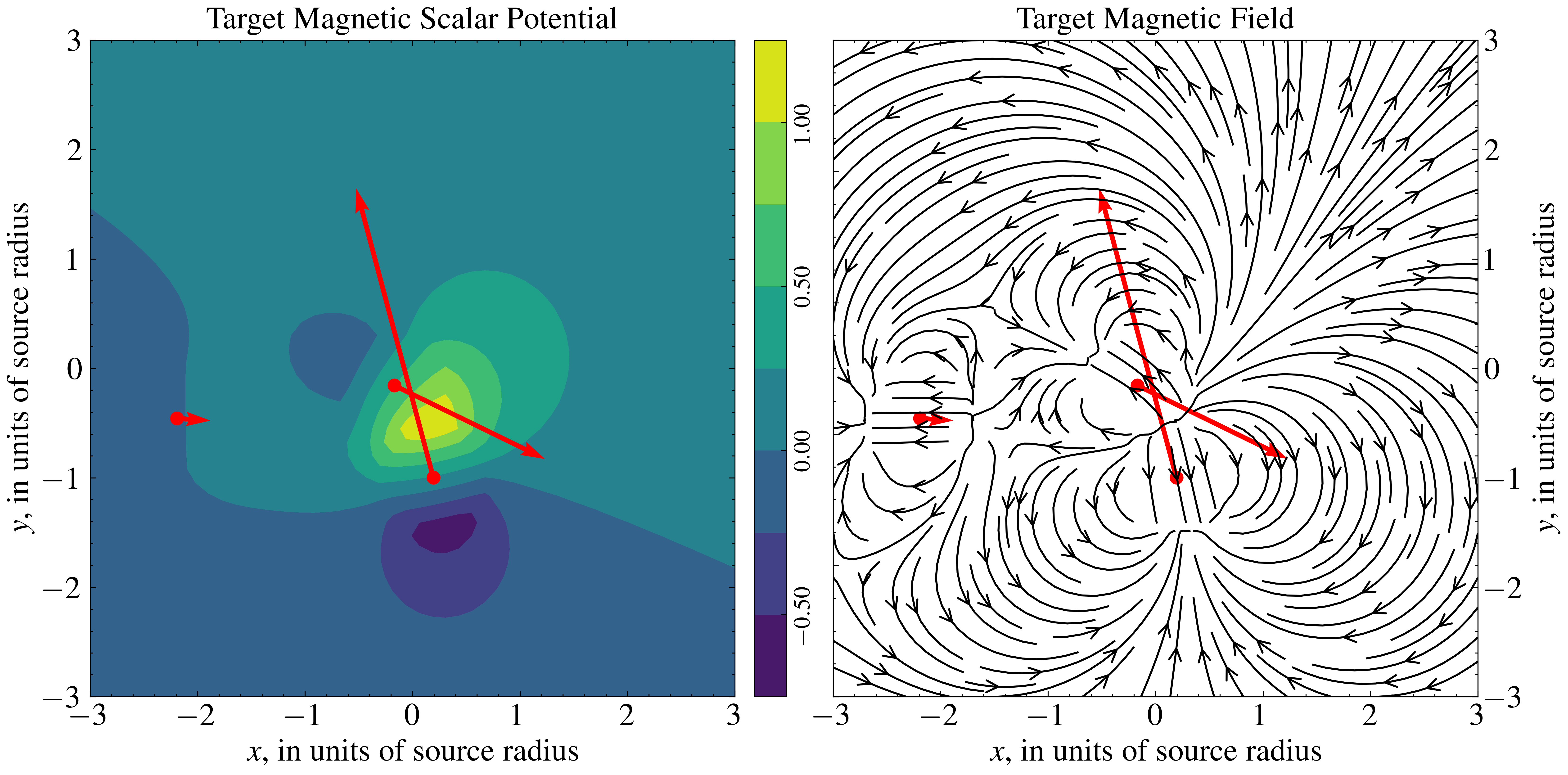
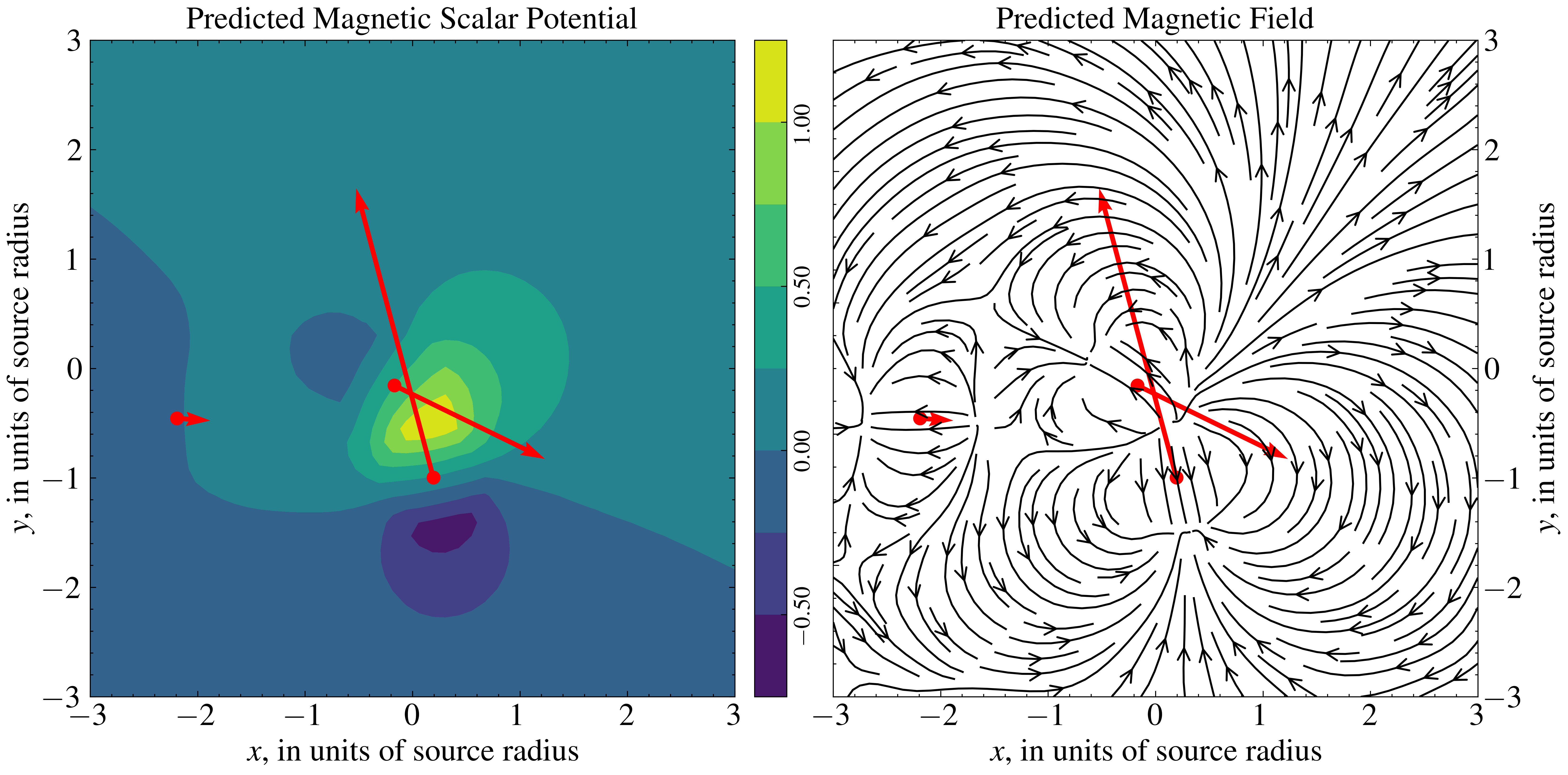
Figure 2: Magnetic potential and field for three finite circular sources (left) and their approximation by a small fully-connected network (right). Sources with locations and direction and magnitude of the magnetisation shown by the red arrows, are randomly positioned within a $[-3,3]\times[-3,3]$ domain, in units of the source radius, with the potential and field generated on a regular $100^{2}$ grid.

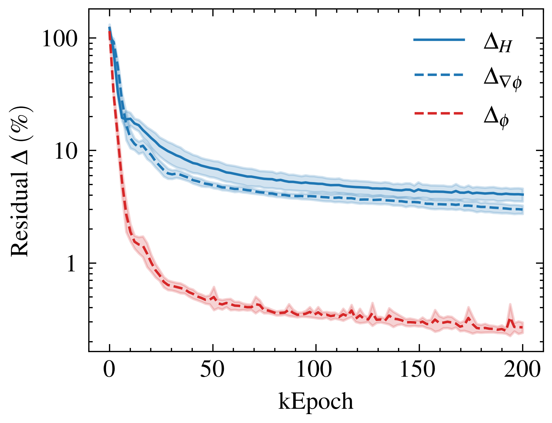
(a)

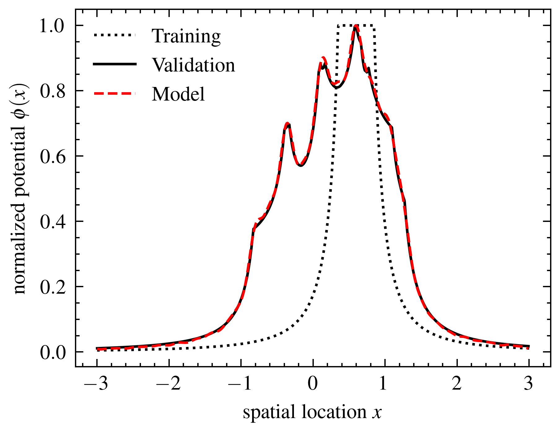
(b)

Figure 3: (Left) Training curves showing error in the predicted magnetic potential (red) and field (blue), per the metrics defined in Eqs. 9, i.e. expressed in % relative error to the target variable. The field evaluations are made directly (solid) and indirectly via the potential (dashed). The shading corresponds to the standard deviation across 10 runs with random model initialization. (Right) The normalized potential as function of position for the training network and a random collection of sources in 1D for the Fourier hypernetwork. Training on examples of a single-source potential (dotted black), the model reproduces the total potential around an arbitrary number of sources (here, 6 are used) placed randomly within the domain.

First, we evaluate how well the architecture can generate the field around a single example of a source collection, without requiring it to learn the dependence on source information, that is, training $f$ while keeping $g$ fixed. In a physical experimental setup, it is only the field and not the potential that can be measured. When training a model to amortize numerical computation, it is possible to train either on fields directly, or on the scalar potentials, which are then numerically differentiated to evaluate performance. It is worth investigating if there benefit to having the model generate the field directly rather than via the potential.

To show how a small fully-connected network $f$ is able to model the potential and field around magnetic sources, we use a single collection of randomly positioned sources, shown in Fig. 2. For this single source collection placed within a $[-3,3]\times[-3,3]$ domain, in units of the source radius, the potential and field are generated on a regular $100^{2}$ grid and using $100^{2}$ randomly sampled locations within the domain for validation. A ensemble of fully-connected networks of width 32 and depth 3 is trained for $10^{5}$ epochs using the Adam optimiser (Kingma & Ba, 2014) with a log learning rate of $-5$. Fig. 3 (left) shows the resulting mean training curves and variance in performance. A model directly inferring the scalar potential ($\Delta_{\phi}$) performs with 0.31% error. The same model can be used to infer the field by taking the numerical gradient of the potential ($\Delta_{\nabla\phi}$, defined in the same way as $\Delta_{H}$ but notated differently to express that the field evaluation is indirect); this reaches an error of 3.70% and notably follows the same training shape. A separate model with the same hidden layer size that directly outputs the magnetic field from the fully-connected network ($\Delta_{H}$) performs comparably to the indirect field method, reaching 4.70% though with an apparently slower convergence. This clearly demonstrates generalisation to arbitrary field locations—but not to arbitrary source collections.

It is unsurprising that, for a given network size and training schedule, the field estimation is less accurate than the potential, given the noising implicit in differentiation. It is also reasonable that a network learning a scalar output can train more easily than one with vector output. As there does not seem to be a justification in accuracy for using the direct field computation, in the following we use the field computation via the potential, as this implies a simpler network architecture and simultaneously lets us evaluate the potential, which is also of intrinsic interest.

5.2 Evaluation of arbitrary source configurations

The previous experiment showed the amortisation ability of a model across the spatial locations at which the field is evaluated, but to achieve the desired scaling performance we must demonstrate how the model generalises jointly across source configurations for the different networks considered. We use an ensemble of $10^{4}$ source collections with randomly generated positions and magnetisations within a $[-3,3]\times[-3,3]$ domain. To exploit the ability of models to superimpose sources, the efficient training strategy is for each collection to be a single source, and we sample each training example at $32^{2}$ uniform random points within the domain. (For visualisation in the figures in this section, a different fixed grid of $128^{2}$ is used.)

While the details of the inference network ($f$) differ depending on the model choice, as described below, for all models we use a fully-connected hypernetwork ($g$) of depth 3 and width equal to the number of parameters to be used by $f$. The networks are trained with a step-wise schedule of Adam optimsers of 5,000 epochs at log learning rates $[-3,-4,-5,-6]$. To facilitate comparison, the model sizes are kept as similar as possible—generally in the range of $\sim$20M trainable parameters—so that the total number of parameter-epochs is approximately constant across the three models. A supplementary Table 3 collates the parameters and configuration used in these experiments.

5.2.1 The Fourier network

For the Fourier network, scaling to an arbitrary number of sources is guaranteed by the linearity of the hypernetwork outputs in the inference network. To present this visually we show in Fig. 3 (right) a model with 32 modes to fit the one-dimensional analogue of the dipole potential, where the model learns only from examples with a single source, and inference can be performed by aggregating weights from many sources before computing the total potential at any position. Performing the training in 1D allows both the training, validation and model to be displayed in the same figure, but the conclusion apply to any dimension. While the generalisation ability of model to arbitrary numbers of sources at arbitrary positions within the domain should not be considered surprising given the architecture, it is an important demonstration of using the principle of superposition to achieve the desired scaling performance at inference time.

The explicit construction of the Fourier model in two dimensions is:

$$\phi(\mathbf{r})\approx\sum_{n}\sum_{m} a_{nm}\cos(\omega_{n}r_{x})\cos(\omega_{m}r_{y})+b_{nm}\sin(\omega_{n}r_{x})\cos(\omega_{m}r_{y})$$ (10)

$$+ c_{nm}\cos(\omega_{n}r_{x})\sin(\omega_{m}r_{y})+d_{nm}\sin(\omega_{n}r_{x})\sin(\omega_{m}r_{y}),$$

where $\omega_{n}=2\pi n/\lambda_{\text{min}}$ is the integer wavenumber, and the sums extend up to a fixed order $N_{\text{max}}$, which is a hyperparameter of training. We use $\omega_{n}=\omega_{m}$ so that the number of parameters generated by the hypernetwork is $\sim N_{\text{max}}^{2}$, making the 2D Fourier expansion of similar size to a linear network layer of width $N_{\text{max}}$. The expansion performs well ($\sim 10\%$) with as few as $N_{\text{max}}=16$ modes in each dimension; 32 modes are used for the metric in Table 2 and inference in Fig. 4.

5.2.2 The FC + ILR model

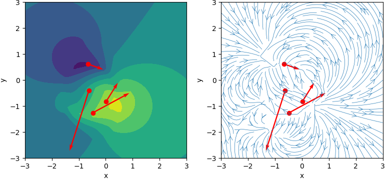
(a) Target

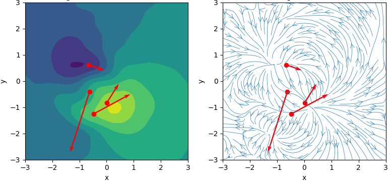
(b) Fourier

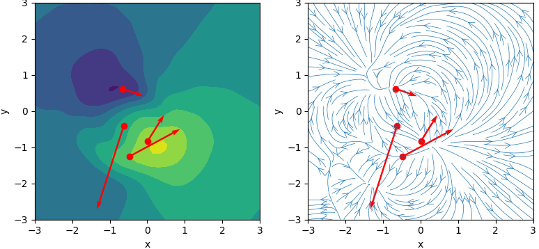
(c) FC + ILR

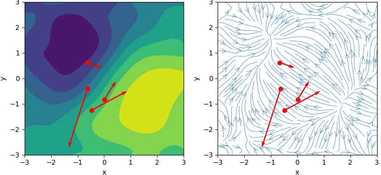
(d) Linear

Figure 4: Multiple source inference on a randomly-selected validation example, using models that learn only on single-source examples. Upper left: Magnetic potential and field from two-dimensional circular magnets at random locations with the domain; Other: The potential and field predicted by the trained models, which are evaluated by first summing the representations for the individual sources, and only then computing the spatial values. The axis and colour map scales are as in Fig. 2.

For the two-dimensional case, Fig. 4 shows the ability of the FC + ILR model to infer the potential and field around finite two-dimensional sources. We emphasise both that i) the training is performed only with single-source examples, and that ii) at inference time the source representations are computed and aggregated before any field evaluation is made.

5.2.3 Linear, exact and FC INR baselines

The more general FC INR network has no guarantee of extending the multiple source data sets when trained only with single source examples. Table 2 collates the validation errors for the different models in 2D, where the source properties and field points are both out-of-sample, with the same model size and training epochs in each case.

	Out-of-sample Error (%; Eq. 9)
Model	Single-source	Multi-source
Fourier	4.74 ($\pm$ 0.38)	5.73 ($\pm$ 0.45)
FC + ILR	4.38 ($\pm$ 0.32)	4.76 ($\pm$ 0.39)
FC INR	3.68	-
Linear	70.0	71.2

Table 2: Out-of-sample error rates for the models, trained over 20,000 epochs, with $1\sigma$ estimates from an ensemble of ten runs with random initialisations. Both the input source properties and the field evaluation locations are chosen out-of-sample. The baseline FC INR model does not have the ability to extend to multiple source data sets when trained only on single-source examples.

An exact numerical baseline, as described in Sec. 2, will have no error, but cannot satisfy the scaling and linearity goals that motivate this work. So we also construct a statistical model baseline: a minimal Linear model where both $f$ and $g$ are linear single layers, with widths extended so that overall model size is the same. This model still satisfies the scaling and superposition required but cannot effectively model the field from the source collection, achieving an error of $\sim 70\%$; an example inference output is shown in Fig 4.

6 Limitations & Discussion

We finish by delineating what this architecture should be capable of in principle, against what we have concretely demonstrated through these experiments. This work develops models that provide inference from arbitrary collections of sources, but our experiments demonstrate this only assuming a particular source shape. For practical results in (e.g.) magnetostatics, it is necessary to develop models in the same architecture trained with shapes like uniformly magnetised prisms and tetrahedra. For data generation, this will require in some cases new analytical derivation of formulae for these shapes, or to use high-resolution simulation to generate data. Developing these models as amortising replacements for infeasible numerical simulation requires extension to three dimensions. All models developed in this paper can be extended to in this way; the Fourier computation will then contain $(2N_{\text{max}})^{3}$ terms, which makes the parameter requirements for the FC + ILR model seem more scalable. We have not explicitly treated equivariance beyond noting a connection between the principle of superposition and permutation invariance of sources.

This work develops models for static configurations. This architecture could be integrated iteratively into a time-varying problem, using the model output to update properties of the sources and then re-evaluating the field. However, it would be more natural to consider training neural operator(s) to evolve the system. This model is most effectively used with collections of sources with spatial extent; for particle-like sources that Fast Multipole Method is a proven non-statistical algorithm with $O(M+N)$ scaling (Greengard & Rokhlin, 1987), with which it would of interest to compare the performance to the method proposed here, in a future work. With the difference of the inclusion of Maxwell’s equation, i.e. the use of harmonic functions and the Fourier model, the same architecture can perform inference for the field around gravitational sources. For work with experimental data, where the field and not the potential is observable, we have demonstrated only the reduced accuracy described in Figure 3 (left), though the potential is practically useful in the context of amortising simulations. Lastly, our particular choice of orthogonal decomposition (7), while physically motivated, may be improved by explicit weighting so that $\lim_{r\to\infty}\phi=0$. These limitations can be addressed with future work, which will be of interest to both the statistics and physics communities.

Code Release

The code for the presented models and experiments is available at this location.

7 Conclusions

Studying the problem of amortising the computation of the field around physical sources, we introduce a general architecture and three models trading off scalability, accuracy of approximation and physical correctness. Modeling via the scalar potential provides benefits to training performance. The Fourier  and FC + ILR models achieve accuracy at the level of $\sim 5\%$, and allow inference of the field around arbitrary numbers of sources by exploiting the physical principle of superposition. The physical motivation of the orthogonal decomposition Fourier model is attractive, but this does not translate into superior approximation, and requires additional tuning and complexity.

Hyperparameters

We have implemented our models using JAX 0.4.25 (Bradbury et al., 2024) and Equinox (Kidger & Garcia, 2021), with training performed on the EuroHPC Karolina GPU cluster. Table 3 collates the model parameters used for the experiments in Sec. 5.

	Fourier	FC + ILR	FC INR
Width	4$\times$32$\times$32	400	20
Depth	-	3	3
HNet Width*	0.25	1.5	1.0
HNet Depth	3	3	2
Total Parameters	6.3M	1.5M	1.7M
Optimiser	Adam
Average Learning Rate	5E–4	1E–4	1E–5
Epochs (thousands)	20	25	20
GPUs	NVIDIA A100-SXM4-40GB
Time (hours)	12	6	–

Table 3: Collation of model parameters used for the experiments in Sec 5 with the architecture developed in this work. A single entry in a row means the same value for all models. *The hypernetwork (hidden layer) width is expressed as a multiple of its output size, which is the total number of learned parameters in the inference network.

The output size of a hypernetwork is the number of parameters consumed by the main (inference) network, and this varies across the models as follows:

• The Fourier model is parameterised by the order $n_{\textrm{max}}$ of the expansion, and in two dimensions its inference ‘network’ requires $4n_{\textrm{max}}^{2}$ parameters;

• In the FC + ILR model, only the final layer of the inference network is set by the hypernetwork, so the total number of learnable parameters is the remaining layers of the inference network plus the hypernetwork size;

• In the FC INR model, the total learnable parameters are those of the hypernetwork, which will quickly have a large output size as the inference network grows. However, because his model does not have the property of linear additivity that allows inference to generalise to multi-source examples, we have not tried to train a large network of this kind.

Consequently, we have found it easiest to express the hypernetwork width in units of its output size. The total number of parameters across both networks is then listed separately.

Tuning tactics for the Fourier model

To coax strong performance from the Fourier architecture, we use the following tactics, which run contrary to intuitions about Fourier series for sampled data:

Selection of modes.

Our intuition for reconstructing a signal from sampled data would follow the constraints on wavelengths for the FFT—the shortest mode is set by the Nyquist sampling frequency and the longest mode is set by the domain window size. In fact, the domain size is irrelevant here because the underlying function is not periodic, and the modes should be significantly longer. In practice, we let the upper and lower bounds for the modes be free parameters, and use a logarithmically-spaced sequence (of length the order of the expansion), affixing the zero-frequency mode to automatically include the Fourier bias terms.

Irregularity of data sampling.

The periodic Fourier modes mean that training on a regular grid encourages overfitting: the reconstruction oscillates wildly even a short distance from the node points. Good practice would in any event suggest that training with data that are irregularly sampled over the domain would be more reliable, and this is the case.

Joint fitting of potential and field.

Given the practical interest in the field resulting from the model output, we find improved performance using a loss with a term for the target potential and an equally-weighted term fit to the target field, evaluated via the gradient of the potential.

References

- Abert et al. (2013) Abert, C., Exl, L., Bruckner, F., et al. magnum.fe: A micromagnetic finite-element simulation code based on fenics. Journal of Magnetism and Magnetic Materials, 345:29–35, 2013. ISSN 0304-8853. doi: https://doi.org/10.1016/j.jmmm.2013.05.051. URL https://www.sciencedirect.com/science/article/pii/S0304885313004022.
- Aharoni (1998) Aharoni, A. Demagnetizing factors for rectangular ferromagnetic prisms. Journal of Applied Physics, 83(6):3432–3434, March 1998. ISSN 0021-8979, 1089-7550. URL https://doi.org/10.1063/1.367113.
- Bjørk & d’Aquino (2023) Bjørk, R. and d’Aquino, M. Accuracy of the analytical demagnetization tensor for various geometries. Journal of Magnetism and Magnetic Materials, 587:171245, 2023.
- Bjørk et al. (2021) Bjørk, R., Poulsen, E. B., Nielsen, K. K., et al. MagTense: A micromagnetic framework using the analytical demagnetization tensor. Journal of Magnetism and Magnetic Materials, 535:168057, October 2021. URL https://www.sciencedirect.com/science/article/pii/S0304885321003334.
- Bradbury et al. (2024) Bradbury, J., Frostig, R., Hawkins, P., Johnson, M. J., Leary, C., Maclaurin, D., Necula, G., Paszke, A., VanderPlas, J., Wanderman-Milne, S., and Zhang, Q. JAX: composable transformations of Python+NumPy programs, 2024. URL http://github.com/google/jax.
- Cranmer et al. (2020) Cranmer, M., Greydanus, S., Hoyer, S., et al. Lagrangian Neural Networks, July 2020. URL http://arxiv.org/abs/2003.04630. arXiv:2003.04630 [physics, stat].
- Engheta et al. (1992) Engheta, N., Murphy, W., Rokhlin, V., et al. The fast multipole method (fmm) for electromagnetic scattering problems. IEEE Transactions on Antennas and Propagation, 40(6):634–641, 1992. doi: 10.1109/8.144597.
- Ghosh et al. (2023) Ghosh, A., Gentile, A. A., Dagrada, M., et al. Harmonic neural networks. In Proceedings of the 40th International Conference on Machine Learning, Icml’23. JMLR.org, 2023.
- Greengard & Rokhlin (1987) Greengard, L. and Rokhlin, V. A fast algorithm for particle simulations. Journal of Computational Physics, 73(2):325–348, 1987. ISSN 0021-9991. doi: https://doi.org/10.1016/0021-9991(87)90140-9. URL https://www.sciencedirect.com/science/article/pii/0021999187901409.
- Greydanus et al. (2019) Greydanus, S., Dzamba, M., and Yosinski, J. Hamiltonian Neural Networks. In Advances in Neural Information Processing Systems, volume 32. Curran Associates, Inc., 2019. URL https://proceedings.neurips.cc/paper/2019/hash/26cd8ecadce0d4efd6cc8a8725cbd1f8-Abstract.html.
- Griffiths (2013) Griffiths, D. Introduction to Electrodynamics. Pearson, 2013. ISBN 9780321856562. URL https://books.google.dk/books?id=AZx_zwEACAAJ.
- Ha et al. (2017) Ha, D., Dai, A. M., and Le, Q. V. Hypernetworks. In International Conference on Learning Representations, 2017. URL https://openreview.net/forum?id=rkpACe1lx.
- Hendriks et al. (2021) Hendriks, J., Jidling, C., Wills, A., et al. Linearly Constrained Neural Networks, April 2021. URL http://arxiv.org/abs/2002.01600.
- Jackson (1999) Jackson, J. D. Classical Electrodynamics, 3rd ed. Hoboken, NJ, USA: Wiley, 1999.
- Joseph & Schlömann (1964) Joseph, R. I. and Schlömann, E. Demagnetizing Field in Nonellipsoidal Bodies. Journal of Applied Physics, 36(5):1579–1593, November 1964. ISSN 0021-8979. URL https://doi.org/10.1063/1.1703091.
- Karniadakis et al. (2021) Karniadakis, G. E., Kevrekidis, I. G., Lu, L., et al. Physics-informed machine learning. Nature Reviews Physics, 3(6):422–440, May 2021. ISSN 2522-5820. doi: 10.1038/s42254-021-00314-5. URL https://www.nature.com/articles/s42254-021-00314-5.
- Kidger & Garcia (2021) Kidger, P. and Garcia, C. Equinox: neural networks in JAX via callable PyTrees and filtered transformations. Differentiable Programming workshop at Neural Information Processing Systems 2021, 2021.
- Kingma & Ba (2014) Kingma, D. P. and Ba, J. Adam: A method for stochastic optimization. arXiv preprint arXiv:1412.6980, 2014.
- Liang et al. (2023) Liang, T.-O., Koh, Y. H., Qiu, T., et al. Magtetris: A simulator for fast magnetic field and force calculation for permanent magnet array designs. Journal of Magnetic Resonance, 352:107463, 2023.
- Müller (2023) Müller, E. H. Exact conservation laws for neural network integrators of dynamical systems. Journal of Computational Physics, 488:112234, 2023. ISSN 0021-9991. doi: https://doi.org/10.1016/j.jcp.2023.112234. URL https://www.sciencedirect.com/science/article/pii/S0021999123003297.
- Nielsen & Bjørk (2020) Nielsen, K. K. and Bjørk, R. The magnetic field from a homogeneously magnetized cylindrical tile. Journal of Magnetism and Magnetic Materials, 507:166799, August 2020. URL https://www.sciencedirect.com/science/article/pii/S0304885319342155.
- Nielsen et al. (2019) Nielsen, K. K., Insinga, A. R., and Bjørk, R. The Stray and Demagnetizing Field of a Homogeneously Magnetized Tetrahedron. IEEE Magnetics Letters, 10:1–5, 2019.
- Ortner & Coliado Bandeira (2020) Ortner, M. and Coliado Bandeira, L. G. Magpylib: A free python package for magnetic field computation. SoftwareX, 2020. doi: 10.1016/j.softx.2020.100466.
- Pollok et al. (2023) Pollok, S., Olden-Jørgensen, N., Jørgensen, P. S., et al. Magnetic Field Prediction Using Generative Adversarial Networks. Journal of Magnetism and Magnetic Materials, 571:170556, April 2023. URL http://arxiv.org/abs/2203.07897.
- Rahimi & Recht (2007) Rahimi, A. and Recht, B. Random features for large-scale kernel machines. In Platt, J., Koller, D., Singer, Y., and Roweis, S. (eds.), Advances in Neural Information Processing Systems, volume 20. Curran Associates, Inc., 2007. URL https://proceedings.neurips.cc/paper%5Ffiles/paper/2007/file/013a006f03dbc5392effeb8f18fda755-Paper.pdf.
- Raissi et al. (2019) Raissi, M., Perdikaris, P., and Karniadakis, G. E. Physics-informed neural networks: A deep learning framework for solving forward and inverse problems involving nonlinear partial differential equations. Journal of Computational Physics, 378:686–707, February 2019. ISSN 0021-9991. doi: 10.1016/j.jcp.2018.10.045. URL https://www.sciencedirect.com/science/article/pii/S0021999118307125.
- Richter-Powell et al. (2022) Richter-Powell, J., Lipman, Y., and Chen, R. T. Q. Neural Conservation Laws: A Divergence-Free Perspective, December 2022. URL http://arxiv.org/abs/2210.01741. arXiv:2210.01741 [cs].
- Schaffer et al. (2023) Schaffer, S., Schrefl, T., Oezelt, H., et al. Physics-informed machine learning and stray field computation with application to micromagnetic energy minimization. Journal of Magnetism and Magnetic Materials, 576:170761, June 2023. URL https://www.sciencedirect.com/science/article/pii/S0304885323004109.
- Sitzmann et al. (2020) Sitzmann, V., Martel, J., Bergman, A., Lindell, D., and Wetzstein, G. Implicit neural representations with periodic activation functions. Advances in neural information processing systems, 33:7462–7473, 2020.
- Slanovc et al. (2022) Slanovc, F., Ortner, M., Moridi, M., Abert, C., and Suess, D. Full analytical solution for the magnetic field of uniformly magnetized cylinder tiles. Journal of Magnetism and Magnetic Materials, 559:169482, 2022.
- Smith et al. (2010) Smith, A., Nielsen, K. K., Christensen, D. V., et al. The demagnetizing field of a nonuniform rectangular prism. Journal of Applied Physics, 107(10):103910, May 2010. URL https://doi.org/10.1063/1.3385387.
- Toth et al. (2020) Toth, P., Rezende, D. J., Jaegle, A., et al. Hamiltonian Generative Networks. In International Conference on Learning Representations, April 2020. URL https://openreview.net/forum?id=HJenn6VFvB.
- Zaheer et al. (2017) Zaheer, M., Kottur, S., Ravanbakhsh, S., et al. Deep sets. In Guyon, I., Luxburg, U. V., Bengio, S., Wallach, H., Fergus, R., Vishwanathan, S., and Garnett, R. (eds.), Advances in Neural Information Processing Systems, volume 30. Curran Associates, Inc., 2017. URL https://proceedings.neurips.cc/paper%5Ffiles/paper/2017/file/f22e4747da1aa27e363d86d40ff442fe-Paper.pdf.