Addressing Unboundedness in Quadratically-Constrained Mixed-Integer Problems

Abstract

Quadratically-constrained unbounded integer programs hold the distinction of being undecidable [1], suggesting a possible soft-spot for Mathematical Programming (MP) techniques, which otherwise constitute a good choice to treat integer or mixed-integer (MI) problems. We consider the challenge of minimizing MI convex quadratic objective functions subject to unbounded decision variables and quadratic constraints. Given the theoretical weakness of white-box MP solvers to handle such models, we turn to black-box meta-heuristics of the Evolution Strategies (ESs) family, and question their capacity to solve this challenge. Through an empirical assessment of quadratically-constrained quadratic objective functions, across varying Hessian forms and condition numbers, we compare the performance of the CPLEX solver to state-of-the-art MI ESs, which handle constraints by penalty. Our systematic investigation begins where the CPLEX solver encounters difficulties (timeouts as the search-space dimensionality increases, $D\gtrsim 30$), on which we report by means of detailed analyses. Overall, the empirical observations confirm that black-box and white-box solvers can be competitive, especially when the constraint function is separable, and that two common ESs’ mutation operators can effectively handle the integer unboundedness. We also conclude that conditioning and separability are not intuitive factors in determining the complexity of this class of MI problems, where regular versus rough landscape structures can pose mirrored degrees of challenge for MP versus ESs.

Keywords: Unbounded integer programs; evolution strategies; integer mutation distributions;
CMA-ES with Integer Handling; ILOG-CPLEX; undecidability.

1 Introduction

Global optimization is a fundamental task across a wide range of disciplines, which is concerned with locating the absolute best objective function value within a region that was predefined by constraints. When the analytical forms of the objective function and constraints are known, the problem is classified as a White-Box Optimization (WBO) problem, which can be solved in a bottom-up manner by utilizing the explicit problem structure and available data. For instance, in numerical optimization, if the continuous objective function is convex and and certain conditions are satisfied, exact solvers can guarantee a solution to the problem [2]. At the same time, problems with non-convex objective functions have been shown to be NP-hard, making them more difficult to solve [3]. In contrast, when no information about the objective function is known, the optimization problem is referred to as a Black-Box Optimization (BBO) problem. In practical optimization problems, a blending of WBO and BBO approaches, referred to as gray-box optimizers [4] or hybrid metaheuristics [5], are frequently encountered. Also, a scheme of BBO problems with so-called explicit constraints, where the constraints are unveiled while the objective function remains black-boxed, is another form of blending that has received attention recently [6]. Notably, the distinction between BBO and WBO is also evident through model-based optimization, which targets BBO problems by constructing explicit surrogates and treating them by WBO solvers. A recent study successfully brought this target to fruition on constrained discrete BBO problems [7]. WBO is typically approached by formal algorithms and Mathematical Programming (MP) techniques, which are rooted in Theoretical Computer Science [8, 9]. Randomized search heuristics, which are a commonly used approach for solving BBO problems [10], operate by evaluating candidate solutions and using the resulting function values to guide the selection of future search points. They serve as a viable alternative to exact solvers, especially on non-convex landscapes. Evolution Strategies (ESs) [11, 12] are a family of effective randomized search heuristics for continuous and discrete search-spaces.

Focus

We focus on Mixed-Integer Optimization (MIO) [13, 14, 15, 16], which involves optimizing an objective function subject to constraints that include both continuous and discrete variables. MIO problems are NP-hard already in the linear case (MILP) and finding an optimal solution is often challenging. However, various optimization techniques have been developed to tackle MIO problems, including MP such as branch-&-bound algorithms, branch-&-cut algorithms, relaxations to semidefinite programming [17, 2], constraint programming [16], and meta-heuristics [18, 19, 20]. These techniques can be applied to a wide range of real-world problems, including design optimization, process optimization, hyperparameter optimization, resource allocation, and network design [15, 13]. The definition of the feasible integer search-space by, e.g., box-constraints, or otherwise being unbounded, is fundamental in the complexity sense. A striking theorem, proved by Jeroslow half a century ago [1], states that unbounded quadratically-constrained integer programs are undecidable. Accordingly, WBO solvers are challenged in practice by this class of problems. At the same time, the unbounded integer search also has implications on the choice of meta-heuristics from the BBO perspective. In particular, it eliminates the possibility to employ standard Genetic Algorithms [21], which require to encode the feasible space by means of fixed-size bitstrings, or any other meta-heuristic that requires explicit boundaries for its operation (e.g., the so-called CMA-ES with “Margins” [22] (cma-wM)).

Contribution

MI ESs (MIESs) were already investigated three decades ago by Rudolph [23] and Bäck [24], and yet, the research outcome of this MIES thread has not widely developed for most years, with a limited number of published studies [25, 26, 15], while enjoying a growing interest only recently [27, 22, 28, 6]. Importantly, certain fundamental questions still remain unanswered, despite the evident success in practice of modern ESs to solve MI problems (e.g., cma-wM [22] for bounded spaces, or another CMA-ES variant, which was adapted to handle integers [28] (cma-IH), for the unbounded case). An open question concerns the effectiveness of employing the normal distribution for integer mutations, in either bounded or unbounded spaces. The contribution of the current study is twofold – (i) assessing whether the theoretical undecidability of unbounded quadratically-constrained MI problems constitutes a WBO weakness, and thus an opportunity for BBO in practice, and (ii) assessing the effectiveness of the ES mutation distribution when handling unbounded integers.

Paper Organization

Next, Section 2 will formally state the problem, distill the research questions and mention the concrete aims. Section 3 will then present the utilized techniques abd specify the experimental setup. The numerical results will be presented in Section 4, and finally, Section 5 will conclude and summarize this study.

2 Problem Statement and Formulation

A standard quadratic program (QP) is formally defined as the minimization of a quadratic objective function whose decision variables are placed within the unit simplex ($\Delta_{D}:=\left\{\vec{x}\in\mathbb{R}_{+}^{D}:\vec{e}^{T}\vec{x}=1\right\}$, with the vector $\vec{e}\in\mathbb{R}^{D}$ of all ones):

$$\textrm{minimize}_{\vec{x}\in\Delta_{D}}\quad\vec{x}^{T}\mathbf{H}\vec{x},$$ (1)

and where $\mathbf{H}$ is a symmetric $D\times D$ real matrix. Non-homogeneous quadratic forms are easily treated by a trivial reformulation [29]. The introduction of integer decision variables renders the problem MI, standardly denoted as MIQP. Solving Eq. 1 is already NP-complete [30] – i.e., this so-called “pure-QP” of continuous variables is a hard problem even before introducing the integer decision variables. When such integers are introduced, the resultant MIQP is clearly a harder computational problem, but progress in addressing it in practice has been achieved [31]. One of the important aspects of the MIQP branch is the fact that it constitutes the next-step from the well-established MILP branch (see, e.g., [32]) toward the generalized Mixed-Integer Nonlinear Programming (MINLP) branch [33]. Finally, another degree of complexity is introduced to the model when the formulation encompasses quadratic constraint terms, and it is then called Quadratically-Constrained QP (QCQP) (also known as all-quadratic programs [34, 35]). In the current context of MI optimization, we will denote such problems as MIQCQP. Quadratic models, either pure-QP or MIQP, arise in a large variety of problems, ranging from Portfolio optimization (Markowitz’s original formulation [36] and its extensions [37]) and resource allocation [38], to population genetics [39] and game theory [40].

2.0.1 WBO: MIQCQP as a Soft-Spot

Jeroslow proved the undecidability of unbounded integer programs with quadratic constraints [1]. Despite this proven problem hardness, there has been much practical progress in treating MIQP in general [31] and MIQCQP in particular (e.g., by reformulation to a bilinear programming problem with integer variables [35], or by diverting to Mixed-Integer Second-Order Cone Programming [41] when the model permits). Although many linearization and reformulation techniques exist [42, 43], a generalized unbounded MIQP cannot be linearized. WBO solvers are typically challenged when treating MIQCQP, an angle that we intend to explore.

2.0.2 BBO: On Integer Mutations and Distributions

Rudolph questioned the suitability of random distributions for evolutionary mutations in unbounded integer spaces [23]. In particular, Rudolph showed that integer mutations utilizing the geometric distribution possess maximum entropy, and demonstrated the effectiveness of such mutations in practice. That study specifically proposed to use the doubly-geometric mutation, which possesses a symmetric distribution with respect to 0. It is achieved by drawing two random variables, $\left\{g_{1},g_{2}\right\}$, according to the geometric distribution $(\jmath=1,2)$: ${\mathbf{Pr}}\left\{g_{\jmath}=k\right\}=p\cdot\left(1-p\right)^{k}$ , and taking their difference, $z=g_{1}-g_{2}$. Importantly, when generalized to the multivariate case of an $n_{z}$-dimensional mutation vector $\vec{z}$, each dimension is drawn individually as such, $\mathcal{G}_{n_{z}}:g_{1}-g_{2}$, yet the distribution as a whole could be controlled by the mean step-size, $S=\mathop{{\mathbb{E}}}\left[\|\vec{z}\|_{1}\right]$:

$$p=1-\frac{S/n_{z}}{\sqrt{\left(1+\left(S/n_{z}\right)^{2}\right)}+1}\quad\Longleftrightarrow\quad S=n_{z}\cdot\frac{2(1-p)}{p(2-p)}.$$ (2)

In practice, each random variable is drawn by the following calculation ($g_{\jmath}$ are the geometrically distributed random variables, both with parameter $p$):

$$\begin{array}[]{l}\displaystyle g_{\jmath}\longleftarrow\left\lfloor\frac{\textrm{log}\left(1-\mathcal{U}\left(0,1\right)\right)}{\textrm{log}\left(1-p\right)}\right\rfloor\quad\jmath=1,2\\ \displaystyle\mathcal{G}_{n_{z}}\left(0,p\right):=g_{1}-g_{2}.\end{array}$$ (3)

The mentioned geometric distribution underlies classical MIESs [24, 25], whereas modern ESs, such as the renowned CMA-ES, were successfully modified to handle integer mutations while maintaining adherence to the normal distribution. We are interested in questioning the effectiveness of these two mutation distributions when handling unbounded integer search.

2.0.3 Research Questions and Concrete Aims

We present our research questions:

Do MIQCQP models constitute a weakness of WBO solvers in practice? How do MIESs compare, as BBO meta-heuristics representatives, in treating such models across different shapes of quadratic forms? And to what extent does the underlying mutation distribution influence their effectiveness?

Overall, we plan to investigate the following family of MI quadratic objective functions with quadratic inequality constraints ($E$ serves as the parametric constraint level):

$$\boxed{\begin{array}[]{ll}\vskip 6.0pt plus 2.0pt minus 2.0pt\displaystyle\textrm{minimize}_{\vec{x}}&f\left(\vec{x}\right):=(\vec{x}-\vec{\xi}_{k})^{T}\cdot\mathcal{H}_{k}\cdot(\vec{x}-\vec{\xi}_{k})\\ \vskip 6.0pt plus 2.0pt minus 2.0pt\displaystyle\textrm{subject to:}&g\left(\vec{x}\right):=(\vec{x}-\vec{\xi}_{\ell})^{T}\cdot\mathcal{H}_{\ell}\cdot(\vec{x}-\vec{\xi}_{\ell})\leq E\\ \displaystyle&\vec{x}\in\mathbb{R}^{D}\\ \displaystyle&x_{i}\in\mathbb{Z}\quad\forall i\in I,\end{array}}$$ (8)

where the $D$-dimensional decision vector $\vec{x}$ is constructed by $n_{r}$ real-valued decision variables followed by $n_{z}$ integer decision variables that are defined by the so-called index set $I:=\left\{n_{r}+1,\ldots,n_{r}+n_{z}\right\}$: $\forall i\in I\quad x_{i}\in\mathbb{Z}$.

3 Approach and Methodology

We would like to conduct a systematic comparison between an exact WBO solver to representative ESs in a fixed-budget (resources) plan. To this end, we consider the commercial CPLEX solver as an MP exact method (and particularly as an MIQCQP solver), versus two MIESs. We begin this section by shortly presenting the techniques, and then describing our numerical setup.

3.1 Solvers

CPLEX

IBM ILOG CPLEX constitutes a broad MP environment, with a large variety of state-of-the-art algorithms under the hood. Given linear or quadratic optimization models, either pure, mixed-integer or all-integer, it utilizes an automated algorithms selection procedure that guides the engine to employ the most suitable sub-routines (e.g., start solving a pure-LP with the dual-Simplex algorithm, and shift to other techniques when certain conditions arise). In our case (MIQCQP with convex objective and constraint functions [45]), the engine’s default selection is a Branch-&-Cut scheme relying on a QP solver [46].

mies

This ES was originally defined to treat altogether real-valued, integer ordinal, and categorical decision variables. We discard herein the treatment of categorical variables. Like most ESs, its operation is well defined by its self-adaptive mutation operator (Algorithm 1): $\left\{\vec{x},\vec{z}\right\}$ are the real-valued and integer decision vectors, respectively, and $\left\{\vec{s},\vec{q}\right\}$ are their strategy parameters, respectively. The normal distribution plays the dominant role of the real-valued update steps, whereas the integer decision variables are mutated by adding doubly geometrically distributed random numbers, following Eq. 3.

mies::mutate($\vec{x},~{}\vec{s},~{}n_{r},~{}\vec{z},~{}\vec{q},~{}n_{z}$)

  /* real-valued decision variables */

$\mathcal{N}_{g}^{(r)}\leftarrow\mathcal{N}\left(0,1\right),~{}\tau_{g}^{(r)}\leftarrow\frac{1}{\sqrt{2\cdot n_{r}}},~{}\tau_{\ell}^{(r)}\leftarrow\frac{1}{\sqrt{2\cdot\sqrt{n_{r}}}}$

for $i=1,\ldots,n_{r}$ do

       $s_{i}^{\prime}\longleftarrow\max\left(\varepsilon,~{}s_{i}\cdot\exp\left\{\tau_{g}^{(r)}\cdot\mathcal{N}_{g}^{(r)}+\tau_{\ell}^{(r)}\cdot\mathcal{N}\left(0,1\right)\right\}\right)$

       $x_{i}^{\prime}\longleftarrow x_{i}+\mathcal{N}\left(0,s_{i}^{\prime}\right)$

      

end for

  /* integer decision variables */

$\mathcal{N}_{g}^{(z)}\leftarrow\mathcal{N}\left(0,1\right),~{}\tau_{g}^{(z)}\leftarrow\frac{1}{\sqrt{2\cdot n_{z}}},~{}\tau_{\ell}^{(z)}\leftarrow\frac{1}{\sqrt{2\cdot\sqrt{n_{z}}}}$

for $i=1,\ldots,n_{z}$ do

       $q_{i}^{\prime}\longleftarrow\max\left(1,~{}q_{i}\cdot\exp\left\{\tau_{g}^{(z)}\cdot\mathcal{N}_{g}^{(z)}+\tau_{\ell}^{(z)}\cdot\mathcal{N}\left(0,1\right)\right\}\right)$

       $z_{i}^{\prime}\longleftarrow z_{i}+\mathcal{G}_{n_{z}}\left(0,q_{i}^{\prime}\right)$ // see Eq. 3

      

end for

return $\left\{\vec{x}^{\prime},~{}\vec{s}^{\prime},~{}\vec{z}^{\prime},\vec{q}^{\prime}\right\}$

Algorithm 1 The self-adaptive mutation operator utilized by the mies: $\left\{\vec{x},\vec{s}\right\}$ are the real-valued decision variables and strategy parameters, respectively. $\left\{\vec{z},\vec{q}\right\}$ are the integer decision variables and strategy parameters, respectively. $\mathcal{N}$ and $\mathcal{G}$ denote the normal and the geometric distributions, respectively (for the latter see (3)). In our implementation we set $\varepsilon:=10^{-5}$. No boundary constraints are enforced.

cma-IH

The CMA-ES is a modern ES [11] that has enjoyed a broad success in global optimization of continuous problems. Its operation is driven by two mechanisms that statistically learn past mutations: updating the covariance matrix $\mathbf{C}$, which is central to landscape maneuvering, and controlling the step-size $\sigma$. Those mechanisms were originally defined for continuous landscapes, and experienced performance issues when deployed on MI problems. Most dominantly, the major issue was identified as stagnation whenever the discrete decision variables get stuck on the landscape’s integer plateaus, and affect the heuristic’s progress. To remedy this malfunction on MI landscapes, the notion of margins was introduced to fix the probability of mutating to another integer, resulting in the so-called cma-wM [22]. However, this fix requires the explicit mapping of the bounded integer space, and thus becomes irrelevant in the unbounded case. A more simplistic fix for handling integers, which we denote as cma-IH and adopt for our study on unboundedness, treats the stagnation by setting a lower bound on the mutation variances [28]. Importantly, the cma-IH handles the entire set of decision variables by means of a unified covariance matrix, which facilitates the $D$-dimensional normally-distributed mutations $\vec{z}_{k}$, and then applies integer rounding to the variables belonging to the index set $I$:
$\displaystyle\vec{x}^{\prime}_{k}\sim\mathcal{N}(\vec{m},\sigma^{2}\mathbf{C})=\vec{m}+\sigma\cdot\mathcal{N}(\vec{0},\mathbf{C})=\vec{m}+\sigma\mathbf{C}^{\frac{1}{2}}\vec{z}_{k},\quad k=1,\ldots,\lambda$
$\displaystyle x^{\prime}_{k,i}\longleftarrow\texttt{round}\left(x^{\prime}_{k,i}\right)\quad\forall i\in I$.

3.2 Experimental Setup

To address our research questions, we define MIQCQP models on which we will assess the behavior of representative WBO and BBO techniques by means of numerical simulations. We elaborate on the choices made in our setup.

3.2.1 Landscape Choice and Instance Generation

To set up a testing framework, we choose concrete quadratic landscapes, and justify in what follows the selection process. We consider a separable and a non-separable Hessian matrices, which play roles in both the objective and the constraint functions:

1. Cigar: $\left(\mathcal{H}_{\textrm{cigar}}\right)_{11}=1,~{}\left(\mathcal{H}_{\textrm{cigar}}\right)_{ii}=c~{}~{}~{}i=2,\ldots,n$

2. Rotated Ellipse: $\mathcal{H}_{\textrm{RE}}=\mathcal{R}\mathcal{H}_{\textrm{ellipse}}\mathcal{R}^{-1}$ where $\left(\mathcal{H}_{\textrm{ellipse}}\right)_{ii}=c^{\frac{i-1}{n-1}}~{}~{}~{}i=1,\ldots,n$, and $\mathcal{R}$ is the rotation by $\approx\frac{\pi}{4}$ radians in the plane spanned by $(1,0,1,0,\ldots)^{T}$ and $(0,1,0,1,\ldots)^{T}$;

with $c$ denoting a parametric condition number. This choice is justified by the evident challenge that these landscapes introduced to both approaches in practice: Selecting (H-1) was based on preliminary runs with the CPLEX solver which indicated timeouts and thus reflected a WBO challenge. Equivalently, (H-2) introduced major challenges to the MIESs.
Altogether, we investigate the following four test-cases, where $f$ refers to the quadratic objective function and $g$ refers to the quadratic constraint function:

1. Cigar+Cigar: $\mathbf{H}_{f}=\mathbf{H}_{g}=\mathcal{H}_{\textrm{cigar}}$

2. RotEllipse+Cigar: $\mathbf{H}_{f}=\mathcal{H}_{\textrm{RE}},~{}\mathbf{H}_{g}=\mathcal{H}_{\textrm{cigar}}$

3. Cigar+RotEllipse: $\mathbf{H}_{f}=\mathcal{H}_{\textrm{cigar}},~{}\mathbf{H}_{g}=\mathcal{H}_{\textrm{RE}}$

4. RotEllipse+RotEllipse: $\mathbf{H}_{f}=\mathbf{H}_{g}=\mathcal{H}_{\textrm{RE}}$

3.2.2 Concrete Calculations

We consider an equal portion of continuous versus discrete decision variables, $D:=n_{r}+n_{z}=2\cdot n$. We set the following points in $\mathbb{R}^{D}$ about which the quadratic models are centered:

$$\displaystyle\vec{\xi}_{0}:= \left(+7,-7,+7,-7,...,+7,-7\right)^{T}$$

$$\displaystyle\vec{\xi}_{1}:= \left(-4,+4,-4,+4,...,-4,+4\right)^{T}.$$

For the separable Cigar, we construct the $D\times D$-dimensional Hessian matrix as a concatenation of two $n\times n$-dimensional matrices, in order to introduce the conditioning effect to both types of variables:

$$\mathbf{H}:=\begin{pmatrix}\mathcal{H}\quad\mathbf{0}\\ ~{}\\ \mathbf{0}\quad\mathcal{H}\end{pmatrix}.$$

Once the $D\times D$-dimensional Hessian matrix is set per the objective function $f$ (denoted as $\mathbf{H}_{f}$) as well as per the constraint function $g$ (denoted as $\mathbf{H}_{g}$), their values are calculated as follows ($\vec{y}_{k}$ denote the translated $\vec{x}$ with respect to $\vec{\xi}_{k}$):

$$\displaystyle f=\frac{1}{c}\cdot\vec{y}_{0}^{T}\mathbf{H}_{f}\vec{y}_{0},\quad \displaystyle\quad g=\frac{1}{c}\cdot\vec{y}_{1}^{T}\mathbf{H}_{g}\vec{y}_{1}.$$ (9)

Importantly, the MIESs handle the constraint function $g$ by means of a penalty term, and practically treat the following cost function:

[BBO cost function:] $$\quad f+10^{4}D^{2}\cdot\Theta(g-E)\cdot(g-E)^{2}\mapsto\min,$$ (10)

where $\Theta$ denotes the Heaviside step function.

3.2.3 Preliminary: Mixed-Integer Sphere-constrained-by-Sphere

We conducted preliminary runs to simulate WBO problem-solving by CPLEX of the simplest MIQCQP instance, subject to various parabolic levels, $E=\{10,30,50,80\}$, across increasing dimensionalities, $D=\{4,8,16,32,64\}$, each limited to 1 hour:

$$\displaystyle\textrm{minimize}_{\vec{x}}~{}~{}\vec{y}_{0}^{T}\cdot\vec{y}_{0}\quad \displaystyle\quad\displaystyle\textrm{subject to: }\vec{y}_{1}^{T}\cdot\vec{y}_{1}\leq E.$$ (11)

We summarize the outcome of these preliminary runs in Table 1. Evidently, the CPLEX solver is challenged on this MIQCQP test-case as of dimension $D=32$, when it occasionally terminates upon exceeding the time-limit. We therefore set up our experiments to consider this dimension as a starting point.

Table 1: CPLEX preliminary runs on the Sphere-constrained-by-Sphere case (Eq. 11). The entries specify the optimization outcome within a time-limit of 1 computation hour – optimal: an optimal solution was attained; tolerance: a solution was located within the relative gap tolerance; and time-out when exceeded the time-limit without indication regarding optimality of the candidate solution.

Dimen.	$E=10$	$E=30$	$E=50$	$E=80$
$D=4$	optimal	optimal	optimal	optimal
$D=8$	optimal	tolerance	tolerance	optimal
$D=16$	tolerance	tolerance	tolerance	tolerance
$D=32$	time-out	tolerance	tolerance	time-out
$D=64$	time-out	time-out	tolerance	tolerance

3.2.4 Problem Instances

To generate concrete problem instances (i.e., instantiate $k$ and $\ell$ in Eq. 8), and given the preliminary runs, we decided to explore three dimensions, $D=\{32,64,128\}$, with constraints level, $E=\{10,30,50,80\}$, across six conditioning, $c=\{10,100,\ldots,10^{6}\}$. Considering the double-Hessian combinations, this setup yields altogether 96 problem instances per dimension.

3.2.5 Numerical Setup

Adhering to a fixed-budget plan, we designate similar computational resources for each method: 1 hour per problem instance at $D=\{32,64\}$, and 2 hours at $D=128$. However, due to the ESs’ stochasticity, we allow a single CPLEX run versus 10 MIESs’ stochastic runs (each granted a budget of $10^{6}$ function evaluations, which was doubled at $D=128$).
Next, we provide the technical specifications of our numerical simulations.

WBO Setup

IBM ILOG CPLEX Optimization Studio 12.8 facilitated the WBO problem solving, modeled and run in OPL. All the experiments were run using the Python API (for sequential execution) and executed on Windows Intel(R) Xeon(R) CPU E5-1620 v4 @ 3.50GHz with 16 processing units. The relative MIP optimality gap was set to $10^{-3}$ (cplex.epgap = 0.001), and the polish procedure [47] was enabled after reaching an integer solution.

BBO Setup

The MIESs were implemented in python3; our mies implementation and parameter settings typically followed [26], whereas the cma-IH was deployed using the pycma package (version 3.3.0) with the default integer handling option. Preliminary runs indicated that the recombination operator was disruptive for the mies, so it was disabled. All runs were deployed on Linux Intel(R) Xeon(R) CPU E5-4669 v4 @ 3.0GHz with 88 processing units.

4 Numerical Results

4.1 Benchmark on MIQCQP Test Problems

We report on the numerical outcome of the simulations prescribed in Section 3.2 and analyze them. We focus on presenting the results per $D=64$, and explicitly mention observations per $D=32$ and $D=128$ only when they exhibited different trends. In terms of performance, it is important to note that the CPLEX terminates due to time-out throughout the test-cases, except for the high conditioning (TC-3) instances, on which it terminated instantly with a status tolerance. Figure 1 provides statistical boxplots of the objective function values, subject to minimization, obtained by the stochastic MIESs when normalized with respect to the deterministic CPLEX (that is, the value of 1.0 always represents the result attained by CPLEX): the separable Cigar as the constraint function [(TC-0),(TC-1)] (depicted in Fig. 1[A,B,E,F]) and the non-separable RotEllipse [(TC-2),(TC-3)] (depicted in Fig. 1[C,D]) serving in that role. The boxplots are group-organized according to the constraint level $E$ (see $x$-axis’ ticks) and group-colored according to the 6 conditioning levels (see legends) – with 24 boxplots per each ES. Next, we elaborate on each test-case.

Figure 1: A gallery of statistical boxplots of the MIESs’ objective function values normalized with respect to CPLEX. Multi-arrow heads represent boxplots with extreme magnitudes (indicative of high degree of divergence). Mind should be given to the $y$-scale, which is not uniform across the gallery. Outliers are depicted as black circles. The boxplots are group-organized according to the constraint level $E$ (see $x$-axis’ ticks) and group-colored according to the conditioning $c$. For each constraint level $E$, the mies boxplot groups are juxtaposed on the left-hand side to the cma-IH boxplot groups.

[A]  (TC-0) (Cigar+Cigar) at $D=64$	[B]  (TC-1) (RotEllipse+Cigar) at $D=64$
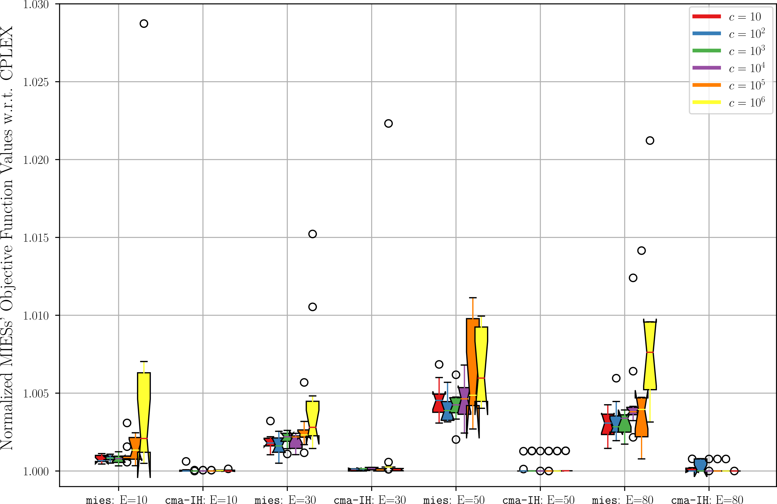
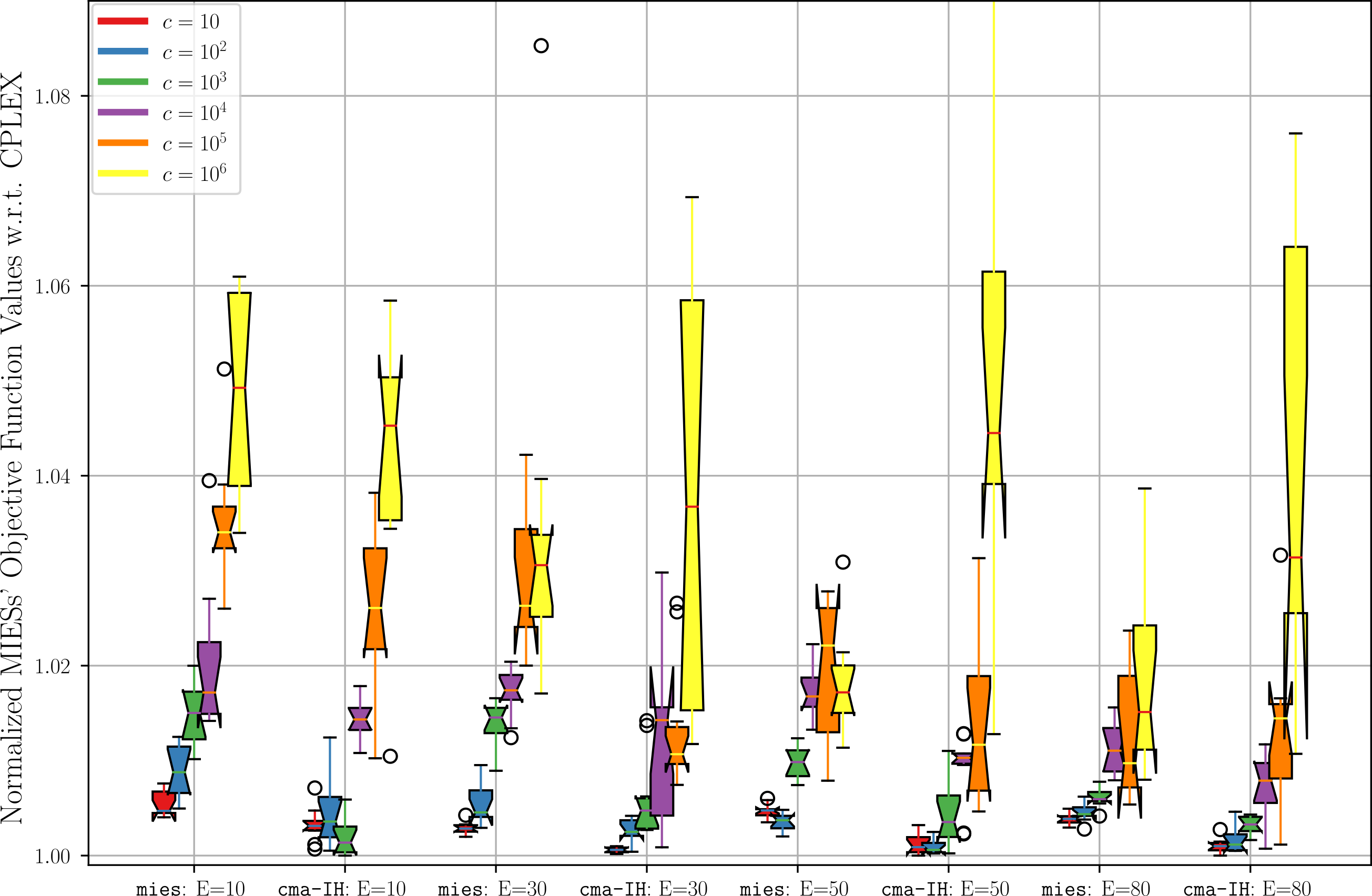
[C]  (TC-2) (Cigar+RotEllipse) at $D=64$	[D]  (TC-3) (RotEllipse+RotEllipse) at $D=64$
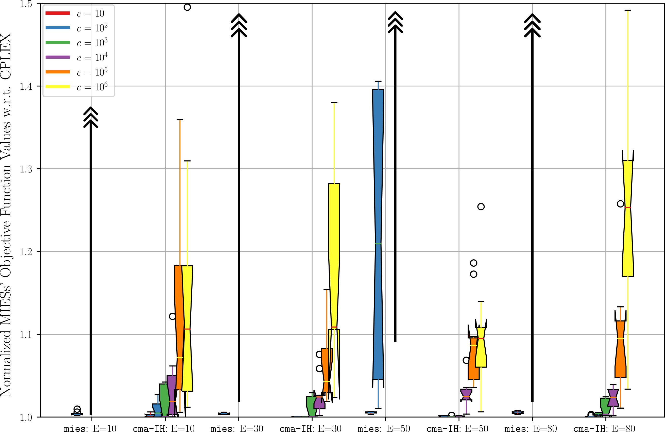
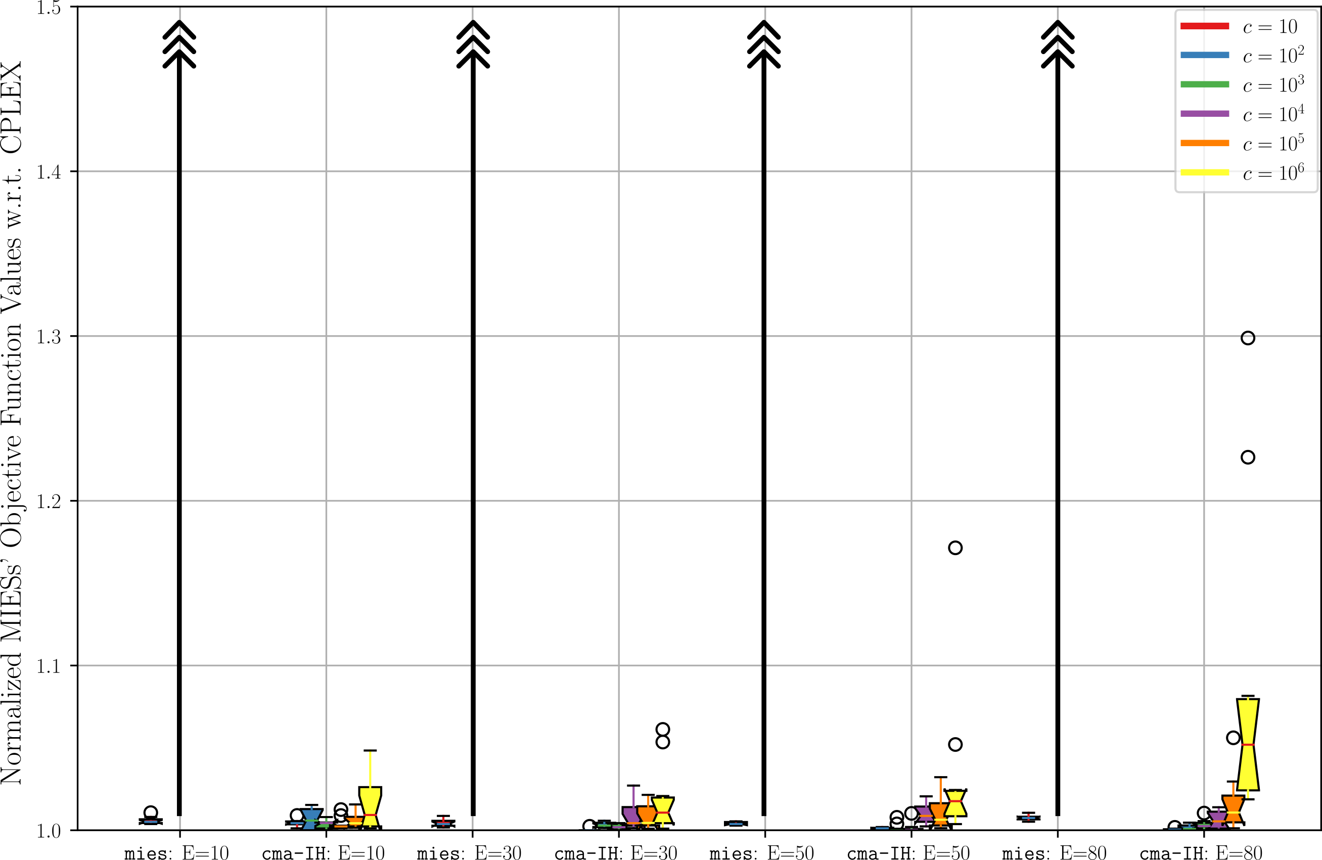
[E]  (TC-0) (Cigar+Cigar) at $D=128$	[F]  (TC-1) (RotEllipse+Cigar) at $D=32$

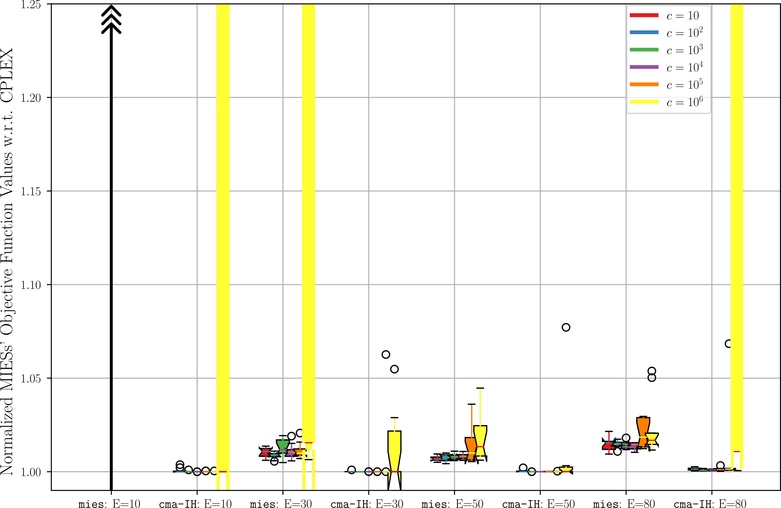
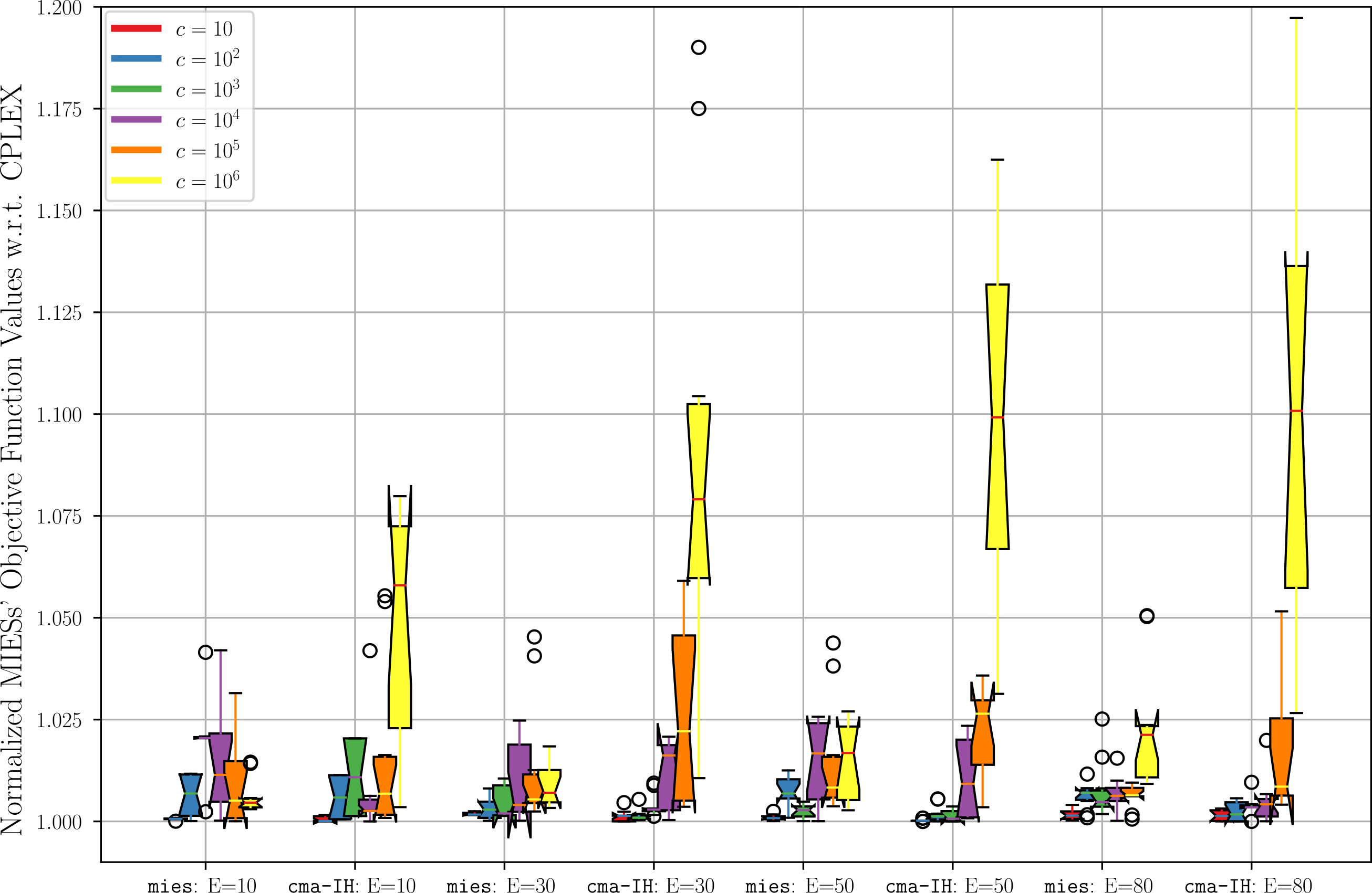
(TC-0) In high level, as evident in Fig. 1[A], the three techniques perform similarly (the reader should mind the limited $y$-scale). That is, the MIESs performed very well compared to the CPLEX and usually attained objective function values within 1% away from the global optima. The cma-IH always performs better, but within an insignificant margin of $\frac{1}{2}$%.
Concerning resources, the CPLEX always terminated due to time-out, whereas the cma-IH did not exploit its budgets entirely (termination due to tolerance criteria). In fact, the cma-IH often terminates on this test-case within 1min, yielding altogether a population of 10 accurate runs much faster than the CPLEX.
Notably, the performance trend per $D=128$ is different (exhibited in Fig. 1[E]): the mies poorly performs throughout $E=10$ and suffers from occasional failures on $c=10^{6}$ per $E=30$, whereas the cma-IH also suffers from occasional failures on $c=10^{6}$ per $E=\{10,80\}$ – in all cases, no more than 3 bad runs. Notably the median runs for those cases remain within small gaps to the CPLEX.

(TC-1) The mies and the cma-IH performed equally well on this test-case, but their attained objective function values have deteriorated with respect to the CPLEX to gaps in the order of 5% (Fig. 1[B]). The cma-IH was challenged by the ill-conditioned instances of $c=10^{6}$, on which it performed slightly worse than the mies when $E=\{30,50,80\}$.
Interestingly, this trend is even more amplified at $D=32$ (depicted in Fig. 1[F]), where the cma-IH does not perform smoothly when the conditioning is $10^{5}$ and higher, and performs strictly worse than the mies on $c=10^{6}$ across all $E$ levels.

(TC-2) The mies exhibited fine performance only on the low conditioning case of $c=10$ across all $E$ levels, and otherwise performed poorly. In practice, it often failed to satisfy the constraint function and remained within the infeasible region throughout many runs. At the same time, the performance of the cma-IH was excellent on the low conditioning instances $c=\{10,100\}$, and has consistently declined with the increasing conditioning to objective function gaps in the order of 10% (when considering the median run; see the median bars of $c=\{10^{5},10^{6}\}$ in Fig. 1[C]). Overall, this seems to be the hardest test-case for the cma-IH in terms of the attained objective function values.

(TC-3) Equivalently to (TC-2), the mies performed well only on the low conditioning case of $c=10$ across all $E$ levels, and otherwise performed poorly, often being penalized for not satisfying the constraint function. The cma-IH, on the other hand, performed very well on this test-case, far better than (TC-2). Its performance slightly degrades for the high conditioning cases of $c=\{10^{5},10^{6}\}$, but still remains below the 10% gap from the CPLEX. Interestingly, as mentioned above, this use-case constitutes the easiest problem for the CPLEX solver (instant computation with a status tolerance), except for the low conditioning of $c=10$ (where it terminates due to time-out).

4.2 The Integer Precision

When analyzing the numerical results in light of an MIESs comparison, there is always an advantage of the cma-IH with respect to the attained objective function values. The gap is occasionally negligible (e.g., below 1% per (TC-0)), but sometimes prominent (either with statistical significance or without). And yet, due to the mixed-integer nature, and when adhering to our second research question, we are ought to assess the attained degree of precision in terms of the “correct” integers within the converged solutions.
In order to numerically assess the precision of a candidate solution $\vec{\zeta}$ with respect to the integer optimizer $\vec{z}^{*}$ (i.e., the subset of integer decision variables at the global optimum ), we introduce a normalized error-rate $\epsilon_{z}\in[0,1]$ which simply counts the miscalculated variables belonging to the index set I:

$$\displaystyle\epsilon_{z}\left(\vec{\zeta},\vec{z}^{*}\right):= \displaystyle\frac{\#\left\{i:\zeta_{i}\neq z_{i}^{*},~{}\forall i\in I\right\}}{n_{z}}~{}.$$ (12)

Care should be given when inspecting this error-rate on multimodal landscapes that possess sub-optimal solutions of high-quality. Figure 2 presents the boxplots of the error-rate $\epsilon_{z}$ for the investigated test-cases. As evident in Fig. 2[A], the two MIESs obtain similar integer error-rates for (TC-0). The constraint level of $E=30$ seems more challenging. Next, when examining (TC-1), this trend of similar error-rates is kept until the high conditioning of $c=\{10^{5},10^{6}\}$, on which the trend flips and the mies obtains lower integer error-rates with statistical significance (see Fig. 2[B]). Per (TC-2), the error-rate pattern is equivalent to the objective function values’ pattern, that is, the mies performs well only on $c=10$, while the cma-IH performs well, with diminishing precision along the increasing conditioning (see Fig. 2[C]). Finally, (TC-3) exhibits a complex pattern of error-rates, which is rooted in the multimodality of this search landscape. The cma-IH accomplishes fine objective function values (see Fig. 1[D]), and yet its located optimizers reside far away from the global optima (see Fig. 2[D]). Interestingly, solutions obtained by the mies are located within moderate error-rates from the global optima whenever it is successful ($c=10$).

We conclude that the objective function advantage of the cma-IH is rooted in its ability to accomplish better precision for the continuous part of the optimizers. The mies seems to identify the correct integers of the optimizers for (TC-0) and (TC-1), but to lack precision of the continuous part on these two test-cases. Altogether, the two MIESs seem competitive in addressing the unbounded integer search, but the mies seems to accomplish higher precision whenever it is able to tackle the problem. We will discuss it further in Section 5.

Figure 2: A gallery of statistical boxplots of the integer error-rate $\epsilon_{z}$ (12) at $D=64$ uniformly scaled by $[0,1]$. The boxplots are group-organized according to the constraint level $E$ and group-colored according to the conditioning $c$; outliers are depicted as black circles.

[A]  (TC-0) (Cigar+Cigar)	[B]  (TC-1) (RotEllipse+Cigar)
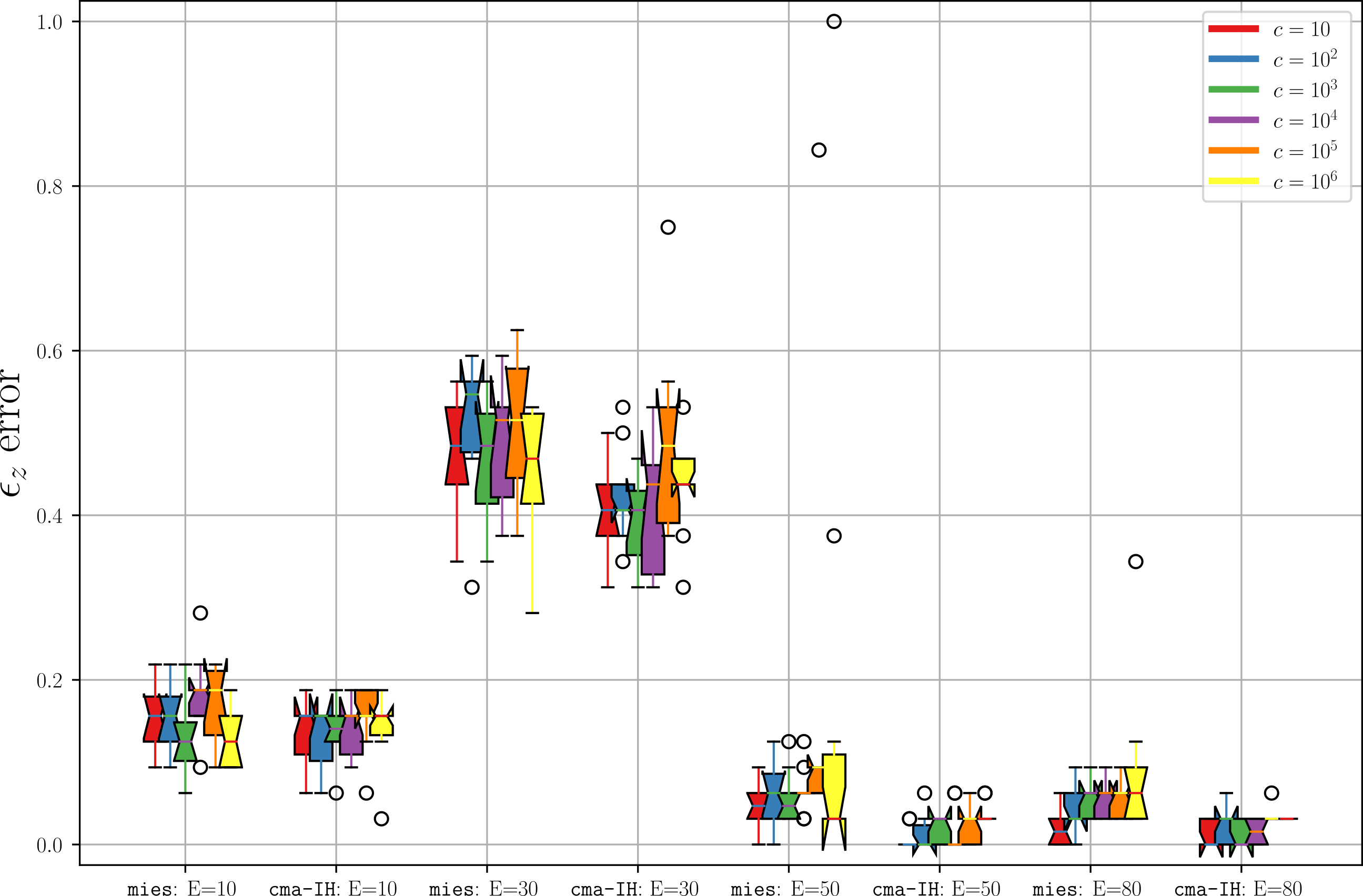
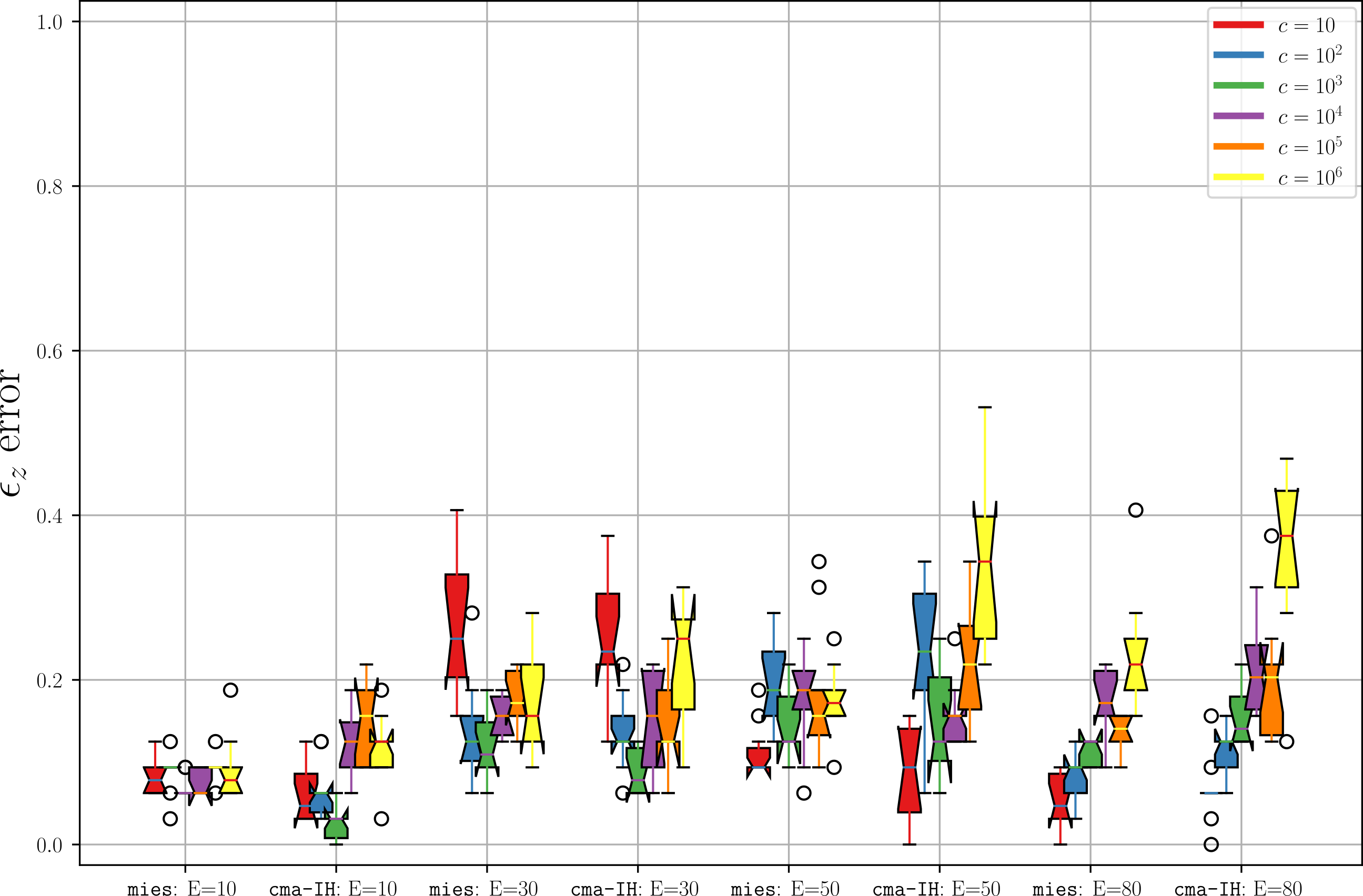
[C]  (TC-2) (Cigar+RotEllipse)	[D]  (TC-3) (RotEllipse+RotEllipse)

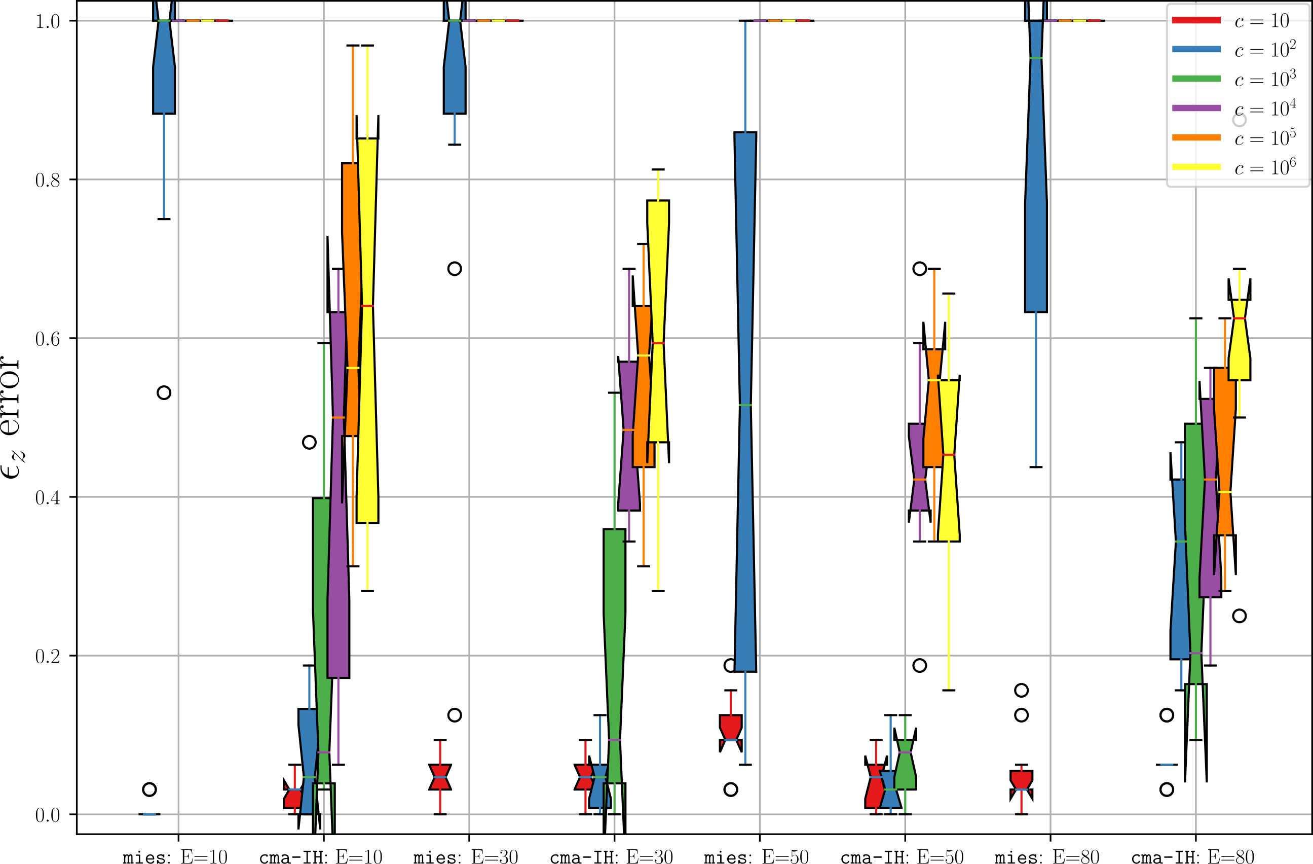
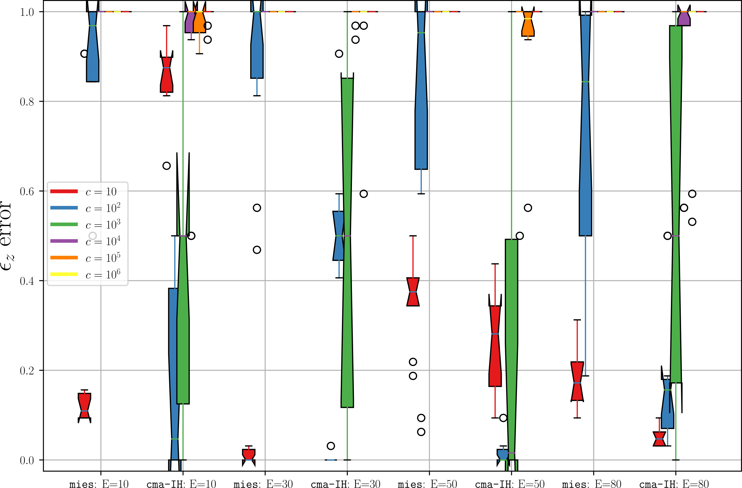
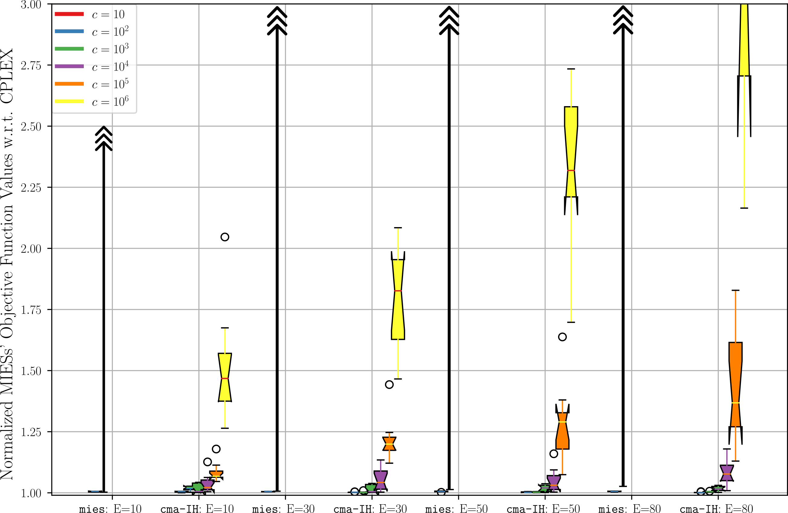
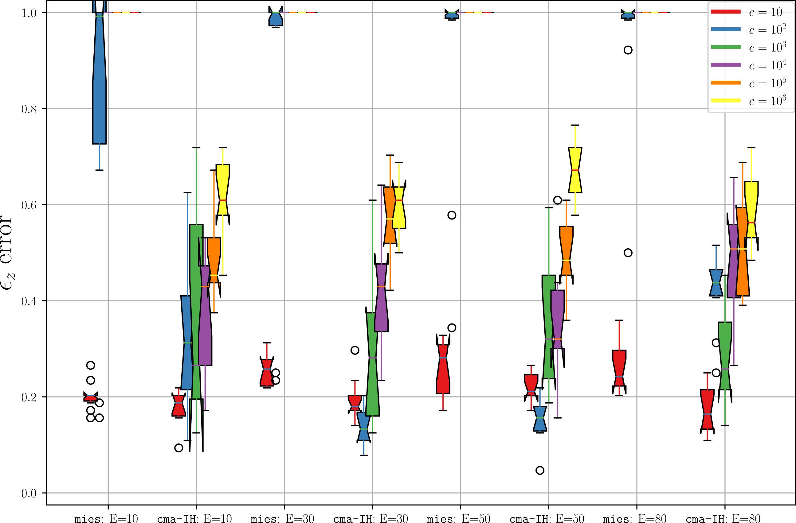
Figure 3: Additional problem-solving of IQCQP (all-integer) at $D=64$, depicting the outcome only for (TC-2) (Cigar+RotEllipse): [LEFT] statistical boxplots of the MIESs’ attained objective function values when normalized with respect to CPLEX, [RIGHT] the integer error-rate $\epsilon_{z}$ (12) per the obtained populations of solutions (decision vectors). Multi-arrow heads represent boxplots with extreme magnitudes. Reference should be made to the mixed-integer problem-solving shown in Fig. 1[C] and Fig. 2[C].

4.3 All-Integer: Additional IQCQP Benchmarking

When turning to IQCQP instances (all-integer problems with equivalent specifications: $D=n_{z}=64,~{}n_{r}=0$), the observed statistical trends are consistent with the mixed-integer patterns shown earlier. It is evident that the two MIESs experience the same strengths and weaknesses when solving the all-integer problems. Due to space limitations, Fig. 3 presents the outcome per (TC-2) alone, comprising boxplots of the objective function values and the integer error-rates. Consistent with the mixed-integer trends shown in Fig. 1[C] and Fig. 2[C], the observed statistical patterns exhibit further amplification for the cma-IH (see $y$-scale), which is challenged by this problem at most.

5 Discussion and Summary

The proven undecidability of MIQCQP problems posed the basis of the current study, which given this potential weakness, addressed research questions involving WBO and BBO approaches targeting that class of problems. Our empirical study focused on the strengths and limitations of the WBO CPLEX solver versus two BBO MIESs. We looked at three main factors of problem complexity: the constraints level (“parabolic tightness”), the interaction between decision variables (separability), and the conditioning of the Hessian matrix of the objective functions. These difficulties were represented in a set of four selected test-cases, which were scalable in terms of constraint-leveling and conditioning. Next, we summarize the key takeaways of our study:

1. The CPLEX solver is significantly challenged by MIQCQP problems with unbounded integer decision variables, but always provides optima of the best quality (even if obtained in timeouts). It experiences difficulties when the search landscape possesses a regular/adequate structure (Cigar across all conditioning), and on the other hand, smoothly handles landscapes with rough multimodal structures (high-conditioned RotEllipse).

2. The two MIESs were shown to treat unbounded integer search very well, relying on their self-adaptive mutation operators. The comparison between the mies to the cma-IH was unfair in the first place, since the former lacks the ability to produce correlated mutations, which strongly underlies the latter. Accordingly, the mies could not treat well the non-separable landscapes, especially when high-conditioned, unlike the cma-IH, which performed well but was challenged in integer precision when high-conditioned.

3. The cma-IH always completes 10 sequential runs with precise results on the Cigar+Cigar prior to the 1 hour time-limit of a single CPLEX run.

4. Integer mutations using the double-geometric distribution showed great potential when examining the integer error-rates of solutions obtained by the mies. Future research should investigate the effectiveness of this distribution when in concert with a correlation mechanism in order to handle the non-separable landscapes. Also, the mies could benefit from a stronger strategy for the continuous search, even on separable landscapes.

5. The cma-IH performed at its best whenever the two Hessian matrices coincided, $\mathbf{H}_{f}=\mathbf{H}_{g}$. This is to be expected when the cost function (10) encapsulates two Hessian matrices, even if the penalty term is a squared form of one of them (yielding a quartic polynomial of $\vec{x}$ with a quadratic term). That is, convergence is effectively achieved when the mutation operator reaches its full potential upon successfully learning an accurate covariance matrix, which coherently addresses the two components of the cost function.

Evidently, it is not a clear cut decision whether to employ the WBO CPLEX or the BBO MIESs, since their relative performance largely depends on the characteristics of the quadratic forms. Finally, conditioning and separability are not intuitive factors in determining the MIQCQP complexity, where regular versus rough structures can pose mirrored degrees of challenge for WBO versus BBO.

References

- [1] R. G. Jeroslow, “There cannot be any algorithm for integer programming with quadratic constraints,” Operations Research, vol. 21, no. 1, pp. 221–224, 1973.
- [2] S. Boyd and L. Vandenberghe, Convex Optimization. New York: Cambridge University Press, 2004.
- [3] P. M. Pardalos and S. A. Vavasis, “Quadratic programming with one negative eigenvalue is NP-hard,” Journal of Global optimization, vol. 1, no. 1, pp. 15–22, 1991.
- [4] D. Whitley, “Next generation genetic algorithms,” in Proceedings of the Genetic and Evolutionary Computation Conference Companion, GECCO ’17, (New York, NY, USA), pp. 922–941, ACM, 2017.
- [5] C. Blum and G. R. Raidl, Hybrid Metaheuristics: Powerful Tools for Optimization. Artificial Intelligence: Foundations, Theory, and Algorithms, Switzerland: Springer International Publishing, 2016.
- [6] Y. Hong and D. Arnold, “Evolutionary mixed-integer optimization with explicit constraints,” in Proceedings of the Genetic and Evolutionary Computation Conference, GECCO ’23, (New York, NY, USA), p. 822–830, Association for Computing Machinery, 2023.
- [7] T. P. Papalexopoulos, C. Tjandraatmadja, R. Anderson, J. P. Vielma, and D. Belanger, “Constrained discrete black-box optimization using mixed-integer programming,” in Proceedings of the 39th International Conference on Machine Learning (K. Chaudhuri, S. Jegelka, L. Song, C. Szepesvari, G. Niu, and S. Sabato, eds.), vol. 162 of Proceedings of Machine Learning Research, pp. 17295–17322, PMLR, 17–23 Jul 2022.
- [8] C. H. Papadimitriou and K. Steiglitz, Combinatorial Optimization: Algorithms and Complexity. Dover Books on Computer Science, Mineola, NY, USA: Dover Publications, 1998.
- [9] C. Moore and S. Mertens, The Nature of Computation. Oxford, UK: Oxford University Press, 2011.
- [10] I. Wegener, Randomized Search Heuristics as an Alternative to Exact Optimization, pp. 138–149. Berlin, Heidelberg: Springer Berlin Heidelberg, 2004.
- [11] T. Bäck, C. Foussette, and P. Krause, Contemporary Evolution Strategies. Natural Computing Series, Springer-Verlag Berlin Heidelberg, 2013.
- [12] M. Emmerich, O. M. Shir, and H. Wang, Handbook of Heuristics, ch. Evolution Strategies, pp. 1–31. Cham: Springer International Publishing, 2018.
- [13] C. A. Floudas, Nonlinear and mixed-integer optimization: fundamentals and applications. New York, NY, USA: Oxford University Press, 1995.
- [14] N. V. Sahinidis, “Mixed-integer nonlinear programming 2018,” 2019.
- [15] R. Li, M. T. Emmerich, J. Eggermont, T. Bäck, M. Schütz, J. Dijkstra, and J. H. Reiber, “Mixed integer evolution strategies for parameter optimization,” Evolutionary Computation, vol. 21, no. 1, pp. 29–64, 2013.
- [16] J. F. Franco, M. J. Rider, and R. Romero, “A mixed-integer quadratically-constrained programming model for the distribution system expansion planning,” International Journal of Electrical Power & Energy Systems, vol. 62, pp. 265–272, 2014.
- [17] W. J. Cook, W. H. Cunningham, W. R. Pulleyblank, and A. Schrijver, Combinatorial Optimization. New York, NY, USA: John Wiley and Sons, 2011.
- [18] G. Rozenberg, T. Bäck, and J. N. Kok, eds., Handbook of Natural Computing: Theory, Experiments, and Applications. Berlin-Heidelberg, Germany: Springer-Verlag, 2012.
- [19] J. Kacprzyk and W. Pedrycz, eds., Springer Handbook of Computational Intelligence. Berlin, Heidelberg: Springer Berlin Heidelberg, 2015.
- [20] R. Martí, P. Pardalos, and M. G. Resende, eds., Handbook of Heuristics. Switzeland: Springer International Publishing, 2018.
- [21] D. Goldberg, Genetic Algorithms in Search, Optimization, and Machine Learning. Reading, MA: Addison Wesley, 1989.
- [22] R. Hamano, S. Saito, M. Nomura, and S. Shirakawa, “CMA-ES with margin: lower-bounding marginal probability for mixed-integer black-box optimization,” in Proceedings of the Genetic and Evolutionary Computation Conference, GECCO ’22, (New York, NY, USA), p. 639–647, Association for Computing Machinery, 2022.
- [23] G. Rudolph, “An Evolutionary Algorithm for Integer Programming,” in Parallel Problem Solving from Nature-PPSN III, pp. 139–148, Springer, 1994.
- [24] T. Bäck and M. Schütz, “Evolution Strategies for Mixed Integer Optimization of Optical Multilayer Systems,” in Evolutionary Programming IV – Proc. Fourth Annual Conf. Evolutionary Programming, pp. 33–51, The MIT Press, 1995.
- [25] R. Li, J. Eggermont, O. M. Shir, M. Emmerich, T. Bäck, J. Dijkstra, and J. Reiber, “Mixed-Integer Evolution Strategies with Dynamic Niching,” in Parallel Problem Solving from Nature - PPSN X, vol. 5199 of Lecture Notes in Computer Science, pp. 246–255, Springer, 2008.
- [26] E. Reehuis and T. Bäck, “Mixed-integer evolution strategy using multiobjective selection applied to warehouse design optimization,” in Proceedings of the 12th annual conference on Genetic and evolutionary computation, GECCO ’10, (New York, NY, USA), pp. 1187–1194, ACM, 2010.
- [27] T. Tušar, D. Brockhoff, and N. Hansen, “Mixed-integer benchmark problems for single- and bi-objective optimization,” in Proceedings of the Genetic and Evolutionary Computation Conference, GECCO ’19, (New York, NY, USA), p. 718–726, Association for Computing Machinery, 2019.
- [28] T. Marty, Y. Semet, A. Auger, S. Héron, and N. Hansen, “Benchmarking CMA-ES with basic integer handling on a mixed-integer test problem suite,” in Proceedings of the Companion Conference on Genetic and Evolutionary Computation, GECCO ’23 Companion, (New York, NY, USA), p. 1628–1635, Association for Computing Machinery, 2023.
- [29] J. Gondzio and E. A. Yildirim, “Global solutions of nonconvex standard quadratic programs via mixed integer linear programming reformulations,” Journal of Global Optimization, vol. 81, pp. 293–321, 2021.
- [30] S. A. Vavasis, “Quadratic programming is in NP,” Information Processing Letters, vol. 36, no. 2, pp. 73–77, 1990.
- [31] C. Bliek, P. Bonami, and A. Lodi, “Solving Mixed-Integer Quadratic Programming problems with IBM-CPLEX: a progress report,” in Proceedings of the 26th RAMP Symposium, Hosei University, Tokyo, 2014.
- [32] E. R. Bixby, M. Fenelon, Z. Gu, E. Rothberg, and R. Wunderling, “MIP: Theory and practice — closing the gap,” in System Modelling and Optimization (M. J. D. Powell and S. Scholtes, eds.), (Boston, MA), pp. 19–49, Springer US, 2000.
- [33] P. Belotti, C. Kirches, S. Leyffer, J. Linderoth, J. Luedtke, and A. Mahajan, “Mixed-integer nonlinear optimization,” Acta Numerica, vol. 22, p. 1–131, 2013.
- [34] U. Raber, “A Simplicial Branch-and-Bound Method for Solving Nonconvex All-Quadratic Programs,” Journal of Global Optimization, vol. 13, pp. 417–432, 1998.
- [35] Y. Zhao and S. Liu, “Global optimization algorithm for mixed integer quadratically constrained quadratic program,” Journal of Computational and Applied Mathematics, vol. 319, pp. 159–169, 2017.
- [36] H. Markowitz, “Portfolio selection,” The Journal of Finance, vol. 7, no. 1, pp. 77–91, 1952.
- [37] P. Bonami and M. A. Lejeune, “An exact solution approach for portfolio optimization problems under stochastic and integer constraints,” Operations Research, vol. 57, no. 3, pp. 650–670, 2009.
- [38] T. Ibaraki and N. Katoh, Resource Allocation Problems: Algorithmic Approaches. Cambridge, MA, USA: MIT Press, 1988.
- [39] J. Kingman, “A mathematical problem in population genetics,” Mathematical Proceedings of the Cambridge Philosophical Society, vol. 57, no. 3, pp. 574––582, 1961.
- [40] I. M. Bomze, “Regularity versus degeneracy in dynamics, games, and optimization: A unified approach to different aspects,” SIAM Rev., vol. 44, no. 3, pp. 394–414, 2002.
- [41] H. Y. Benson and U. Saglam, Mixed-Integer Second-Order Cone Programming: A Survey, ch. Chapter 2, pp. 13–36.
- [42] W. P. Adams, R. J. Forrester, and F. W. Glover, “Comparisons and enhancement strategies for linearizing mixed 0-1 quadratic programs,” Discrete Optimization, vol. 1, no. 2, pp. 99–120, 2004.
- [43] M. Asghari, A. M. Fathollahi-Fard, S. M. J. Mirzapour Al-e hashem, and M. A. Dulebenets, “Transformation and linearization techniques in optimization: A state-of-the-art survey,” Mathematics, vol. 10, p. 283, Jan 2022.
- [44] A. Billionnet, S. Elloumi, and A. Lambert, “Linear reformulations of integer quadratic programs,” in Modelling, Computation and Optimization in Information Systems and Management Sciences (H. A. Le Thi, P. Bouvry, and T. Pham Dinh, eds.), (Berlin, Heidelberg), pp. 43–51, Springer Berlin Heidelberg, 2008.
- [45] IBM ILOG, “MIQCP: mixed integer programs with quadratic terms in the constraints.” https://www.ibm.com/docs/, 2021.
- [46] M. J. Best, Quadratic Programming with Computer Programs. Advances in Applied Mathematics, Boca Raton FL, USA: CRC Press, 2017.
- [47] E. Rothberg, “An Evolutionary Algorithm for Polishing Mixed Integer Programming Solutions,” INFORMS Journal on Computing, vol. 19, no. 4, pp. 534–541, 2007.