Randomized quasi-Monte Carlo and Owen’s boundary growth condition: A spectral analysis

Abstract

In this work, we analyze the convergence rate of randomized quasi-Monte Carlo (RQMC) methods under Owen’s boundary growth condition [Owen, 2006] via spectral analysis. Specifically, we examine the RQMC estimator variance for the two commonly studied sequences: the lattice rule and the Sobol’ sequence, applying the Fourier transform and Walsh–Fourier transform, respectively, for this analysis. Assuming certain regularity conditions, our findings reveal that the asymptotic convergence rate of the RQMC estimator’s variance closely aligns with the exponent specified in Owen’s boundary growth condition for both sequence types. We also provide analysis for certain discontinuous integrands.

65C05

1 Introduction

The quasi-Monte Carlo (QMC) method utilizes deterministic low-discrepancy sequences (LDS) to compute integrals. The prestigious Koksma–Hlawka inequality indicates that, for integrands whose variation in the Hardy–Krause sense is finite, the QMC integration error is bounded by the product of the Hardy–Krause variation and the star-discrepancy of the point set. The star-discrepancy converges as $\mathcal{O}(N^{-1}(\log N)^{s})$ for the LDS with fixed size $N$ and $\mathcal{O}(N^{-1}(\log N)^{s-1})$ for infinite sequences. However, the Koksma–Hlawka inequality fails to be informative for certain singular integrands in $L^{2}$. For functions with boundary unboundedness, Owen [25] characterizes a boundary growth condition and establishes connections with the asymptotic QMC convergence rates. Meanwhile, [14] finds that problem-specific lattice rules can achieve dimension-independent $\mathcal{O}(N^{-1})$ worst-case convergence rate. Additionally, the work [10] studies the convergence of randomly scrambled Sobol’ sequence for integrands with discontinuities.

The randomized QMC (RQMC) achieves unbiased mean estimators by randomizing the low-discrepancy sequences. The variance of the RQMC estimator has been explored in the previous literature. L’Ecuyer [15] investigates the randomly-shifted lattice rule (RSLR) using the Fourier transform. Owen [21] analyzes Sobol’ sequences through Haar wavelets. An equivalent formulation using the Walsh–Fourier transform is revealed in [5]. In this work, we conduct a spectral analysis of the RQMC estimator variance for both lattice rules and Sobol’ sequences concerning certain types of singular integrands. Assuming these integrands exhibit boundary unboundedness, discontinuities, or both, we leverage Fourier and Walsh–Fourier transforms to investigate their spectral properties.

This paper is organized as follows. Section 2 provides background information and notations related to the RQMC. Section 3 analyzes the RSLR and Sobol’ sequences through spectral analysis. Section 4 further analyzes Sobol’ sequences for discontinuous integrands. Section 5 presents numerical results. Finally, section 6 concludes the paper and discusses possible further directions.

2 Background

In this section, we introduce the lattice rule, Sobol’ sequences, and Owen’s boundary growth condition to characterize the integrand regularity.

2.1 Notations

First, we want to introduce notations that we will use throughout the paper.

$[\bm{a},\bm{b}]$: the hyperrectangle interval $\{\bm{t}\in\mathbb{R}^{s}:\min(\bm{a}_{j},\bm{b}_{j})\leq\bm{t}_{j}\leq\max(\bm{a}_{j},\bm{b}_{j})\}$.

${}_{b}\mathrm{wal}_{\bm{\ell}}$: the Walsh basis with index $\bm{\ell}\in\mathbb{N}_{0}^{s}$ in base $b$.

$c_{\bm{n}}$: the Fourier coefficient of $f$, $\bm{n}\in\mathbb{N}_{0}^{s}$.

$\Delta(f;\cdot,\cdot)$: the alternating sum of $f$.

$\bar{f}(\bm{\ell})$: the Walsh–Fourier coefficient of $f$ with index $\bm{\ell}$.

$\hat{f}$: the Fourier transform of $f$.

$\phi:[0,1]\to\mathbb{R}$ is given by $\phi(t)\coloneqq\min(t,1-t)$. To be used in Owen’s boundary growth condition and derivations.

$\Gamma_{\mathfrak{u},\bm{\ell}}$, $\Gamma_{\bm{\ell}}$: the “gain coefficient” of the digital net, $\mathfrak{u}\subseteq 1:s$, $\bm{\ell}\in\mathbb{N}_{0}^{s}$.

$s\in\mathbb{N}$: the integration dimension. We denote $1:s=\{1,2,\dotsc,s\}$.

$\lesssim$: the inequality holds up to a finite constant, i.e., $a\lesssim b$ means $a\leq Cb$ for some constant $C<+\infty$, $a,b\in\mathbb{R}$.

2.2 Lattice rule

In this work, we will specifically discuss the rank-1 lattice rule: Given a generating vector $\bm{z}\in\mathbb{N}^{s}$, the lattice rule with $N$ quadrature points is given by

(1) $$\left\{i\frac{\bm{z}}{N}\ \textrm{mod}\ 1:i=0,1,\dotsc,N-1\right\}.$$

The lattice rule can be extensible, meaning that when $N$ increases, extra new points can be added to the existing quadrature points without discarding the previously computed points. However, this requires the admissible choices of $N$ to be powers of a fixed integer, such as $N=2^{k}$ with $k\in\mathbb{N}$. Such extensible lattice rules are often addressed as “lattice sequences”.

For optimizing the generating vector $\bm{z}$, refer to [13, 2].

2.3 Sobol’ sequence

We first introduce the definition of a $(t,m,s)$-net in base $b$. A $(t,m,s)$-net in base $b$ is a set of $b^{m}$ points in $[0,1)^{s}$ such that every $s$-dimensional elementary interval

(2) $$E_{\bm{\ell},\bm{k}}=\prod_{j=1}^{s}\left[\frac{\bm{k}_{j}}{b^{\bm{\ell}_{j}}},\frac{\bm{k}_{j}+1}{b^{\bm{\ell}_{j}}}\right)$$

where $\bm{\ell}=(\bm{\ell}_{1},\dotsc,\bm{\ell}_{s})\in\mathbb{N}_{0}^{s}$, $\lvert\bm{\ell}\rvert:=\sum_{j=1}^{s}\bm{\ell}_{j}=m-t$ and $\bm{k}=(\bm{k}_{1},\dotsc,\bm{k}_{s})\in\mathbb{N}_{0}^{s}$ with $\bm{k}_{j}<b^{\bm{\ell}_{j}}$ for $j=1,\dotsc,s$, contains exactly $b^{t}$ points. $t$ is referred to as the quality parameter, $s$ as the dimension and $b^{m}$ as the number of quadrature points. More properties of the $(t,m,s)$-nets can be found in [5]. The Sobol’ sequence is a kind of $(t,m,s)$-nets in base $b=2$. Owen proposed nested uniform scrambling [20] to randomize the Sobol’ sequence, which, however, requires substantial storage and computational cost. Matoušek [17] proposes the random linear scramble as an alternative approach with reduced computational cost, which does not alter the mean squared $L^{2}$ discrepancy. A review of other randomizations can be found in [23].

The parameters in the Sobol’ sequence can be optimized in order to improve the quadrature points quality. For instance, the work [12] optimizes the Sobol’ sequences for better two-dimensional projections.

2.4 Owen’s boundary growth condition

Owen [25] proposes the boundary growth condition to characterize the unbounded integrand $f$ on $[0,1]^{s}$, which is given as follows. [Owen’s boundary growth condition [25]] Let $f\in L^{2}([0,1]^{s})$, and the derivative $\frac{\partial^{\mathfrak{u}}f}{\partial\bm{t}_{\mathfrak{u}}}$ exists on $(0,1)^{s}$ for $\mathfrak{u}\subseteq 1:s$. Then the boundary growth condition is given by

(3) $$\left\lvert\frac{\partial^{\mathfrak{u}}f}{\partial\bm{t}_{\mathfrak{u}}}\right\rvert\leq C\prod_{j=1}^{s}\phi(t_{j})^{-\mathbbm{1}_{j\in\mathfrak{u}}-A_{j}}$$

for all $\mathfrak{u}\subseteq\{1,\dotsc,s\}$, $\max_{j}A_{j}<1/2$ and $\phi:[0,1]\to\mathbb{R}$, $\phi(t)\coloneqq\min(t,1-t)$. Owen [25] proves that for integrands satisfying the condition (3), the RQMC $L^{1}$ convergence rate is given by $\mathcal{O}(n^{-1+\epsilon+A})$ for low-discrepancy sequences, for $\epsilon>0$. He et al. [11] and Gobet et al [6] have derived the RQMC $L^{2}$ convergence rate with $\mathcal{O}(n^{-1+\epsilon+A})$ under additional conditions. The former considers the Sobol’ sequence, while the latter assumes the correlations between randomized QMC quadrature points. In this work, we are interested in the convergence in $L^{2}$ for the lattice rule and Sobol’ sequence. The spectral analysis of these two low-discrepancy sequences, along with the boundary growth condition assumptions, is detailed in Section 3.

3 Spectral Analysis of RQMC and Owen’s boundary growth condition

In this section, we will explore the variance of the RSLR and scrambled Sobol’ sequence using the Fourier and Walsh–Fourier transformations, respectively.

3.1 Lattice Rule

The Fourier transform requires periodicity. Consequently, we consider the torus $\mathbb{T}^{s}=[0,1]^{s}$ and let the integrand $f\in L^{2}(\mathbb{T}^{s})$. The exact integration over this domain is represented by,

(4) $$I=\int_{\mathbb{T}^{s}}f(\bm{t})d\bm{t}.$$

Consider lattice points $\{\bm{t}_{i}\in[0,1]^{s}:i=0,\dotsc,N-1\}$ (1) and a random shift $\bm{\Delta}\sim\mathcal{U}([0,1]^{s})$. The RSLR estimator $I_{N}^{\textrm{lat}}\coloneqq I_{N}^{\textrm{lat}}(f)$ is then defined as

(5) $$I_{N}^{\textrm{lat}}=\frac{1}{N}\sum_{i=0}^{N-1}f({\bm{t}_{i}+\bm{\Delta}}).$$

In the following, we use the Fourier transform to study the variance of the RSLR estimator. Let $\hat{f}:\mathbb{R}^{s}\to\mathbb{C}$ denote the Fourier transform of $f$, expressed as

(6) $$\begin{split}\hat{f}({\bm{\omega}})&=\int_{\mathbb{R}^{s}}f(\bm{t})e^{-i2\pi\bm{\omega}\cdot\bm{t}}d\bm{t}\\ &=\sum_{\bm{n}\in\mathbb{Z}^{s}}c_{\bm{n}}\delta(\bm{\omega}-\bm{n})\end{split}$$

where $\delta$ is the Dirac delta function and the Fourier coefficients $c_{\bm{n}}$ of $f$ are given by

(7) $$c_{\bm{n}}=\int_{\mathbb{T}^{s}}f(\bm{t})e^{-i2\pi\bm{n}\cdot\bm{t}}d\bm{t}.$$

Given $N$ samples $\{\bm{t}_{i}\in[0,1]^{s}:i=0,\dotsc,N-1\}$, we introduce the N-sample operator $S_{N}[\bm{t}]$ and the randomized N-sample operator $S_{N}[\bm{t}+\bm{\Delta}]$ as follows:

(8) $$S_{N}[\bm{t}] \coloneqq\frac{1}{N}\sum_{i=0}^{N-1}\delta_{\bm{t}_{i}},$$

(9) $$S_{N}[\bm{t}+\bm{\Delta}] \coloneqq\frac{1}{N}\sum_{i=0}^{N-1}\delta_{\bm{t}_{i}+\bm{\Delta}},$$

where $\delta_{\bm{t}_{i}}$ and $\delta_{\bm{t}_{i}+\bm{\Delta}}$ are the Dirac function centered at $\bm{t}_{i}$ and $\bm{t}_{i}+\bm{\Delta}$, respectively, with $\bm{\Delta}~{}\mathcal{U}([0,1]^{s})$. Following [27], the integration estimator $I^{\mathrm{lat}}_{N}$ can be written as the inner product between the randomized N-sample operator $S_{N}[\bm{t}+\bm{\Delta}]$ and the integrand $f$, i.e.,

(10) $$\begin{split}I^{\mathrm{lat}}_{N}&=\left\langle S_{N}[\bm{t}+\bm{\Delta}],f\right\rangle_{L^{2}(\mathbb{T}^{s})}\\ &=\int_{\mathbb{R}^{s}}\left({\hat{S}^{N}}_{\bm{\omega}}[\bm{t}+\bm{\Delta}]\right)^{*}\hat{f}({\bm{\omega}})d\bm{\omega}\\ &=\sum_{\bm{n}\in\mathbb{Z}^{s}}\left({\hat{S}^{N}}_{\bm{n}}[\bm{t}+\bm{\Delta}]\right)^{*}c_{\bm{n}}\end{split}$$

where $\left\langle\cdot,\cdot\right\rangle$ denotes the inner product, the Fourier transformation is applied in the second line, ^∗ denotes the complex conjugate, and the third line is a constraint from $\mathbb{R}^{s}$ to $\mathbb{Z}^{s}$. For $\bm{\omega}\in\mathbb{R}^{s}$, the spectral density of the randomized $N$-sample estimator ${\hat{S}^{N}}_{\bm{\omega}}[\bm{t}+\bm{\Delta}]$ is defined by,

(11) $${\hat{S}^{N}}_{\bm{\omega}}[\bm{t}+\bm{\Delta}]\coloneqq\frac{1}{N}\sum_{i=0}^{N-1}\int_{\mathbb{R}^{s}}\delta_{\bm{t}_{i}+\bm{\Delta}}e^{-i2\pi\bm{\omega}\cdot\bm{t}}d\bm{t}=\frac{1}{N}\sum_{i=0}^{N-1}e^{-i2\pi\bm{\omega}\cdot(\bm{t}_{i}+\bm{\Delta})}.$$

We let ${\hat{S}^{N}}_{\bm{n}}[\bm{t}+\bm{\Delta}]$ be a constraint of ${\hat{S}^{N}}_{\bm{\omega}}[\bm{t}+\bm{\Delta}]$ from $\mathbb{R}^{s}$ to $\mathbb{Z}^{s}$. Notice that the exact integration is given by the Fourier coefficient of the zero-frequency component, i.e., $I=c_{0}$.

Lemma 3.1 (Variance of the RSLR estimator [15, 27]).

The variance of the RSLR estimator (5) is given by

(12) $$\mathrm{Var}(I_{N}^{\mathrm{lat}})=\sum_{\bm{n}\in\mathbb{Z}^{s}\setminus\{0\}}{\left\lvert\hat{S}_{\bm{n}}^{N}[\bm{t}]\right\rvert^{2}}\left\lvert c_{\bm{n}}\right\rvert^{2}.$$

The proof to Lemma 12 can be referred to [15] and [27]. For completeness, we provide the proof in Appendix A.

Next, we will introduce two essential notations. The set $\{\bm{h}\in\mathbb{Z}^{s}:\bm{h}\cdot\bm{z}\equiv 0\mod N\}$ is known as the dual lattice to the $N$-point rank-1 lattice rule generated by $\bm{z}$. Figure 1 plots a lattice rule $\bm{z}=(1,13)$, $N=21$ and the corresponding dual lattice.

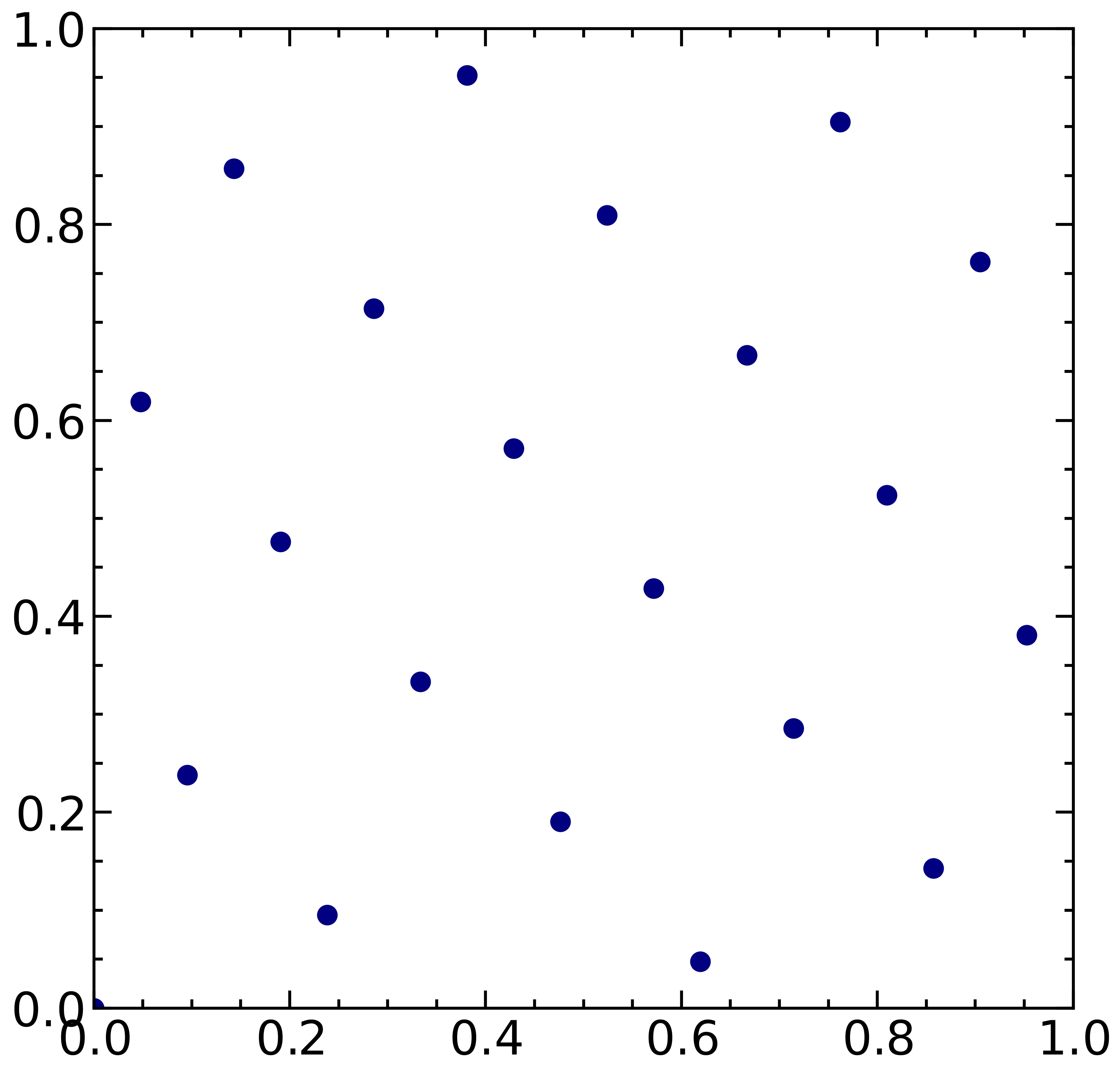
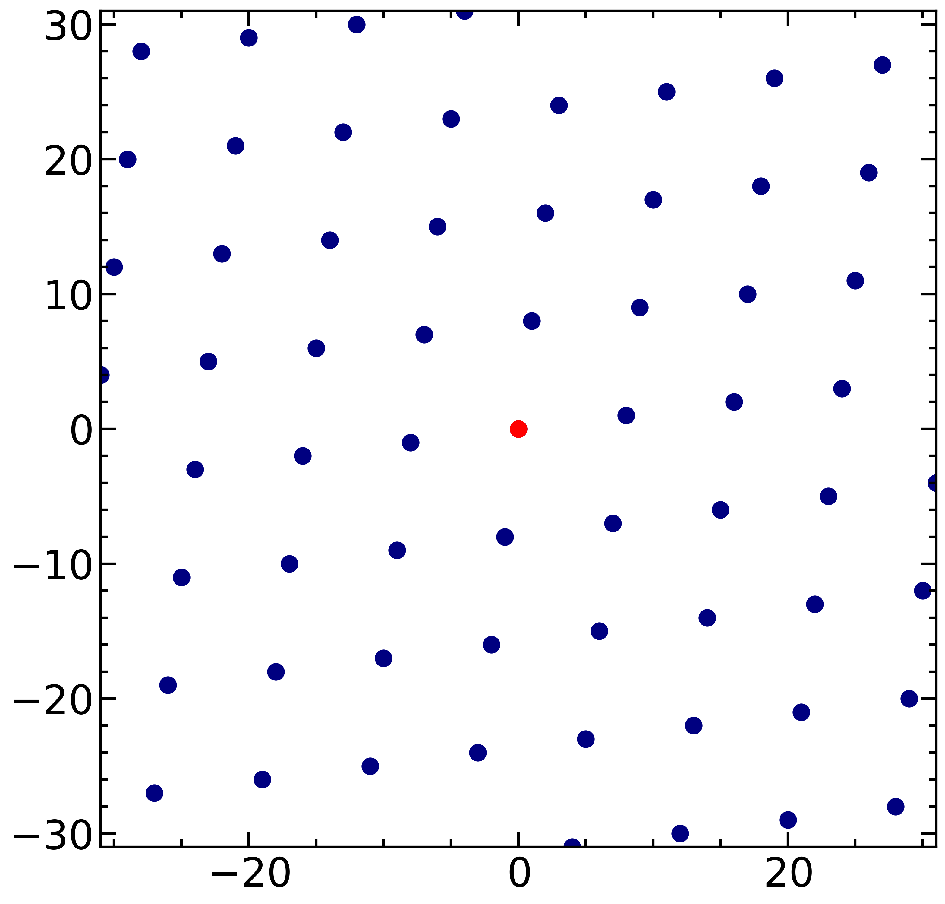
Figure 1: The lattice rule (left) with $\bm{z}=(1,13)$, $N=21$ and the corresponding dual lattice (right). The origin in the dual lattice is marked in red.

We also introduce the power spectral density (PSD) as the expectation of the squared spectral density. For RSLR, since the quadrature $\{\bm{t}_{i}$, $i=1,\dotsc,N\}$ are deterministic, the PSD is given by

(13) $$P_{\textrm{lat}}(\bm{n}):={\left\lvert\hat{S}_{\bm{n}}^{N}[\bm{t}]\right\rvert^{2}}.$$

The property of the PSD and variance for RSLR is given in the following lemma.

Lemma 3.2 (Variance of RSLR estimator [15]).

For the lattice with size $N$ generated by vector $\bm{z}\in\mathbb{N}^{s}$, the PSD for RSLR is given by

(14) $${P_{\mathrm{lat}}}(\bm{n})=\begin{cases}1&\text{if}\ {\bm{n}}\cdot\bm{z}\equiv 0\ \mathrm{mod}\ N,\\ 0&\text{otherwise}.\end{cases}$$

Thus the variance of the RSLR integration estimator, ${\mathrm{Var}\mspace{-2.0mu}\left[I_{N}^{\mathrm{lat}}\right]}$, is given by

(15) $${\mathrm{Var}\mspace{-2.0mu}\left[I_{N}^{\mathrm{lat}}\right]}=\sum_{\begin{subarray}{c}\bm{n}\cdot\bm{z}\equiv 0(\textrm{mod }N),\\ \bm{n}\neq 0\end{subarray}}\left\lvert c_{\bm{n}}\right\rvert^{2},$$

which is the summation of the squared Fourier coefficients of the integrand at the dual lattice except the origin.

The results first appear in [15]. We present an alternative proof in Section B, which does not assume $f\in L^{2}(\mathbb{T}^{s})$.

Remark 3.3 (Monte Carlo PSD).

Notice that in the case of Monte Carlo, the variance of the MC estimator is given by

(16) $${\mathrm{Var}\mspace{-2.0mu}\left[I_{N}\right]}=\frac{1}{N}\sum_{\bm{n}\neq 0}\left\lvert c_{\bm{n}}\right\rvert^{2}.$$

For instance, the reader can refer [27] for derivations. Figure 2 illustrates the decay property of MC and RSLR estimator variance of the unbounded 1-d function $f(t)=\phi(t)^{-0.25}$. The MC estimator variance decays as $\mathcal{O}(N^{-1})$ for all the integer frequencies except 0, which corresponds to the pink color in the plot. The RSLR estimator reduces the variance by discarding certain frequencies, with the orange color in the plot representing an upper bound of the RSLR variance. From Figure 2, it is clear that the convergence of the RSLR estimator variance depends on the decay property of the Fourier coefficients.

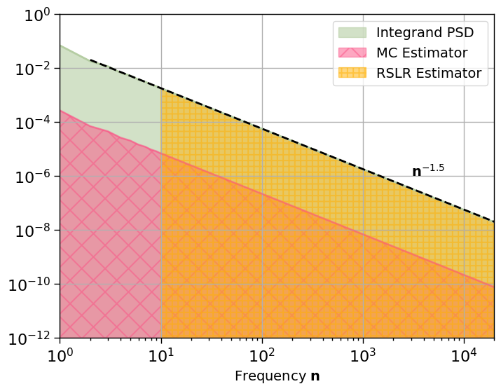
Figure 2: The integrand PSD, MC and RSLR estimator variances for the 1-d function $f(t)=\phi(t)^{-0.25}$.

Remark 3.4 (Fourier coefficients and integration error).

For the lattice rule $\{\bm{t}_{i}\in[0,1]^{s}:i=0,\dotsc,N-1\}$ with a generating vector $\bm{z}\in\mathbb{N}^{s}$, it is also known that the Fourier coefficients play an important role in the integration error for deterministic lattice rule, i.e.,

(17) $${I-\frac{1}{N}\sum_{i=0}^{N-1}f(\bm{t}_{i})}=\sum_{\begin{subarray}{c}\bm{n}\cdot\bm{z}\equiv 0(\textrm{mod }N),\\ \bm{n}\neq 0\end{subarray}}c_{\bm{n}},$$

cf. [18, 5, 4, 3, 28].

Following Niederreiter [18], we introduce the following definition, which characterizes the decay property of the Fourier coefficients.

Definition 3.5.

Given $\bm{n}\in\mathbb{Z}^{s}$, $\alpha>1/2$ and a constant $C<+\infty$, the function class $\mathcal{E}_{\bm{n}}^{\alpha}(C)$ is defined as follows: for $f\in\mathcal{E}_{\bm{n}}^{\alpha}$, its Fourier coefficients $c_{\bm{n}}$ satisfies

(18) $$\lvert c_{\bm{n}}\rvert\leq C\prod_{j=1}^{s}{{r_{1}}{({n}_{j})}^{-\alpha}},\ \bm{n}\neq 0$$

where $r_{1}(n_{j})\coloneqq\max{\{1,\lvert n_{j}\rvert\}}$, for $j=1,\dotsc,s$.

Notice that in definition 3.5, we have extended the range of $\alpha$ from $\alpha>1$ in Niederreiter’s definition [18] to $\alpha>1/2$. For $f\in\mathcal{E}_{\bm{n}}^{\alpha}$, we have the following existance result.

Lemma 3.6.

There exist a generating vector $\bm{z}\in\mathbb{N}^{s}$ such that

(19) $${\mathrm{Var}\mspace{-2.0mu}\left[I_{N}^{\mathrm{lat}}\right]}=\mathcal{O}(N^{-2\alpha}(\log N)^{2\alpha s}).$$

For instance, refer to [4, 18, 3].

Zaremba [29] characterized a sufficient condition for a function $f$ to belong to the space $\mathcal{E}_{\bm{n}}^{\alpha}(C)$: Let $\alpha>1$ be an integer and that all partial derivatives

(20) $$\frac{\partial^{k_{1}+\cdots+k_{s}}f}{\partial t_{1}^{k_{1}}\cdots\partial t_{s}^{k_{s}}}\quad 0\leq k_{j}\leq\alpha-1,\ j=1,\dotsc,s$$

exist and are of bounded variation on $\mathbb{T}^{s}$ in the sense of Hardy–Krause. Then $f\in\mathcal{E}_{\bm{n}}^{\alpha}(C)$ for the constant $C$ given explicitly. In the rest of this section, we characterize the relation between Owen’s boundary growth condition and the decay rate $\alpha$ of Fourier coefficients.

Lemma 3.7.

Consider the one-dimensional function $f:[0,1]\to\mathbb{R}$, with the derivative $\frac{\partial f}{\partial t}$ defined on $(0,1)$, satisfying the boundary growth condition (3) with $0\leq A<1/2$. The Fourier coefficients $c_{n}$ satisfies

(21) $$\lvert c_{n}\rvert=\begin{cases}\mathcal{O}(n^{-1+A})&\text{if}\ 0<A<1/2,\\ \mathcal{O}(n^{-1}\log{n})&\text{if}\ A=0.\end{cases}$$

The proof follows a classic approach to the Riemann–Lebesgue lemma and is deferred to Appendix C.

In the case when ${A}<0$, however, we only achieve the convergence at $\mathcal{O}(n^{-1})$ if we follow the proof in Appendix C. Furthermore, to explore the effect of discontinuities, we propose stronger assumptions on higher-order derivatives in Assumption 3.7. Given $\bar{A}<1$. Let $k\in\mathbb{N}_{0}$. Consider the 1-d function $f:[0,1]\to\mathbb{R}$. We assume that the $(k-1)$-th derivative, $\frac{\partial^{k-1}f}{\partial t^{k-1}}$ is continuous on $\mathbb{T}=[0,1]$, and the $k$-th derivative $\frac{\partial^{k}f}{\partial t^{k}}$ is piecewise continuous on $\mathbb{T}$, admitting finite number of discontinuities, denoted by $0<t_{1}<t_{2}<\cdots<t_{d}\leq 1$, $d<+\infty$. The $(k+1)$-th derivative $\frac{\partial^{(k+1)}f}{\partial t^{k+1}}$ satisfies the boundary growth condition (22) for some $\bar{A}<1$.

(22) $$\left\lvert\frac{\partial^{(k+1)}f}{\partial t^{k+1}}\right\rvert\leq\phi(t)^{-1-\bar{A}}.$$

When $k=0$, we denote

$$\frac{\partial^{-1}f}{\partial t^{-1}}(t_{0})\coloneqq\int_{0}^{t_{0}}f(t)dt.$$

Lemma 3.8.

For function $f$ satisfying Assumption 3.7, we have

(23) $$\lvert c_{n}\rvert=\begin{cases}\mathcal{O}(n^{-1-k}),&\text{if}\ \bar{A}<0\\ \mathcal{O}(n^{-1-k}\log(n)),&\text{if}\ \bar{A}=0\\ \mathcal{O}(n^{-1-k+A}),&\text{if}\ 0<\bar{A}<1.\end{cases}$$

Proof 3.9.

We start with the integration by parts.

(24) $$\begin{split}c_{n}\cdot(-i2\pi n)^{k}&=\int_{0}^{1}(-i2\pi n)^{k}f(t)e^{-i2\pi nt}dt\\ &=-\int_{0}^{1}(-i2\pi n)^{k-1}\frac{\partial f}{\partial t}e^{-i2\pi nt}dt+\underbrace{(-i2\pi n)^{k-1}f(t)e^{-i2\pi nt}\mid_{0}^{1}}_{=0}\\ &\ \vdots\\ &=(-1)^{k}\int_{0}^{1}\frac{\partial^{(k)}f}{\partial t^{k}}e^{-i2\pi nt}dt+\underbrace{\frac{\partial^{(k-1)}f}{\partial t^{k-1}}e^{-i2\pi nt}\mid_{0}^{1}}_{=0}\\ \end{split}$$

where we have applied the continuity of $f$, $\frac{\partial f}{\partial t}$, $\dotsc$, $\frac{\partial^{(k-1)}f}{\partial t^{k-1}}$ on $\mathbb{T}$. Notice that we can use the same technique as in the proof of Lemma 3.7. We have

(25) $$\int_{0}^{1}\frac{\partial^{(k)}f}{\partial t^{k}}(t)e^{-i2\pi nt}dt=-\int_{0}^{1}\frac{\partial^{(k)}f}{\partial t^{k}}\left(t+\frac{1}{2n}\right)e^{-i2\pi nt},$$

and

(26) $$c_{n}\cdot(-i2\pi n)^{k}=\frac{1}{2}\int_{0}^{1}\left(\frac{\partial^{(k)}f}{\partial t^{k}}(t)-\frac{\partial^{(k)}f}{\partial t^{k}}\left(t+\frac{1}{2n}\right)\right)e^{-i2\pi nt}dt.$$

We derive the following upper bound for $\lvert c_{n}\rvert$:

(27) $$\lvert c_{n}\rvert\lesssim{n^{-k}}\int_{0}^{1}\left\lvert\frac{\partial^{(k)}f}{\partial t^{k}}(t)-\frac{\partial^{(k)}f}{\partial t^{k}}\left(t+\frac{1}{2n}\right)\right\rvert dt.$$

When $\bar{A}\geq 0$, we consider the interior discontinuities at $t_{1},\dotsc,t_{d-1}$ with $t_{d-1}<1$. For sufficiently large $n$, when the interval $[t,t+\frac{1}{2n}]$ contains only one discontinuity of $\frac{\partial^{(k)}f}{\partial t^{k}}$, i.e. there exists only one $t_{i}\in[t,t+\frac{1}{2n}]$ for $i=1,\dotsc,d$, we have

(28) $$\left\lvert\frac{\partial^{(k)}f}{\partial t^{k}}(t)-\frac{\partial^{(k)}f}{\partial t^{k}}\left(t+\frac{1}{2n}\right)\right\rvert\leq\int_{t}^{t+\frac{1}{2n}}\left\lvert\frac{\partial^{k+1}f}{\partial t^{k+1}}\right\rvert dt+C_{i}$$

where $C_{i}=\lvert\lim_{t\to t_{i}^{+}}f(t)-\lim_{t\to t_{i}^{-}}f(t)\rvert$ is a constant, for $t_{d}\neq 1$. When $t_{d}=1$ and $t_{d}\in[t,t+\frac{1}{2n}]$, we have

(29) $$\left\lvert\frac{\partial^{(k)}f}{\partial t^{k}}(t)-\frac{\partial^{(k)}f}{\partial t^{k}}\left(t+\frac{1}{2n}\right)\right\rvert\leq\int_{t+\frac{1}{2n}-1}^{t}\left\lvert\frac{\partial^{k+1}f}{\partial t^{k+1}}\right\rvert dt+(d-1)C_{d-1}^{*}.$$

with $C_{d-1}^{*}=\max_{i=1}^{d-1}\lvert\lim_{t\to t_{i}^{+}}f(t)-\lim_{t\to t_{i}^{-}}f(t)\rvert$. Denote $\Omega_{d}=\{\bm{t}\in[0,1):\exists i=1,\dotsc,d,t_{i}\in[t,t+\frac{1}{2n}]\}$, for sufficiently large $n$, we have

(30) $$\begin{split}\lvert c_{n}\rvert&\leq n^{-k}\left(\int_{[0,1]-\Omega_{d}}\int_{[t,t+\frac{1}{2n}]}\left\lvert\frac{\partial^{k+1}f}{\partial t^{k+1}}(t_{0})\right\rvert dt_{0}dt\right.\\ &\quad\quad\quad\left.+\int_{\Omega_{d}}\left\lvert\frac{\partial^{(k)}f}{\partial t^{k}}(t)-\frac{\partial^{(k)}f}{\partial t^{k}}\left(t+\frac{1}{2n}\right)\right\rvert dt\right)\\ &\lesssim n^{-k}\left(\int_{[0,1]-\Omega_{d}}\int_{[t,t+\frac{1}{2n}]}\left\lvert\frac{\partial^{k+1}f}{\partial t^{k+1}}(t_{0})\right\rvert dt_{0}dt\right.\\ &\quad\quad\quad\left.+\int_{\Omega_{d}}\int_{[t,t+\frac{1}{2n}~{}\mathrm{mod}~{}1]}\left\lvert\frac{\partial^{k+1}f}{\partial t^{k+1}}\right\rvert dt+C_{d-1}^{*}dt\right)\\ &\lesssim n^{-k}\left(\int_{[0,1]}\int_{[t,t+\frac{1}{2n}~{}\mathrm{mod}~{}1]}\phi(t_{0})^{-1-\bar{A}}dt_{0}dt+\frac{1}{n}\right).\end{split}$$

Notice that the notation $\int_{[t,t+\frac{1}{2n}~{}\mathrm{mod}~{}1]}$ represents the integration over the interval $[t,t+\frac{1}{2n}]$ or $[t+\frac{1}{2n}-1,t]$, from Section 2.1. When $\bar{A}\geq 0$, the computation of

$$\int_{[0,1]}\int_{[t,t+\frac{1}{2n}~{}\mathrm{mod}~{}1]}\phi(t_{0})^{-1-\bar{A}}dt_{0}dt$$

can be refered to the proof in Appendix C. Next we consider when $\bar{A}<0$, the bound over the discontinuity (28) holds for all $i=1,\dotsc,d$. Similarly, we have

(31) $$\begin{split}\lvert c_{n}\rvert&\leq n^{-k}\left(\int_{[0,1]-\Omega_{d}}\int_{[t,t+\frac{1}{2n}]}\left\lvert\frac{\partial^{k+1}f}{\partial t^{k+1}}(t_{0})\right\rvert dt_{0}dt\right.\\ &\quad\quad\quad\left.+\int_{\Omega_{d}}\left\lvert\frac{\partial^{(k)}f}{\partial t^{k}}(t)-\frac{\partial^{(k)}f}{\partial t^{k}}\left(t+\frac{1}{2n}\right)\right\rvert dt\right)\\ &\lesssim n^{-k}\left(\int_{[0,1]-\Omega_{d}}\int_{[t,t+\frac{1}{2n}]}\left\lvert\frac{\partial^{k+1}f}{\partial t^{k+1}}(t_{0})\right\rvert dt_{0}dt\right.\\ &\quad\quad\quad\left.+\int_{\Omega_{d}}\int_{[t,t+\frac{1}{2n}]}\left\lvert\frac{\partial^{k+1}f}{\partial t^{k+1}}\right\rvert dt+\max_{i=1}^{d}C_{i}dt\right)\\ &\lesssim n^{-k}\left(\int_{[0,1]}\int_{[t,t+\frac{1}{2n}]}\phi(t_{0})^{-1-\bar{A}}dt_{0}dt+\frac{1}{n}\right).\end{split}$$

When $\bar{A}<0$, $\phi(t_{0})^{-1-\bar{A}}$ is integrable on $[0,1]$, i.e.,

$$\int_{[0,1]}\int_{[t,t+\frac{1}{2n}]}\phi(t_{0})^{-1-\bar{A}}dt_{0}dt<+\infty.$$

The conclusion follows.

With Assumption 3.7, Lemma 3.8 generalizes the result of Lemma 3.7. To interpret the result, consider that both the boundary unboundedness and the interior discontinuities can affect the convergence rate. When $\bar{A}\geq 0$, the boundary unboundedness dominates the convergence rate. Conversely, when $\bar{A}<0$, the $k$-th derivative of $f$, $\frac{\partial^{k}f}{\partial t^{k}}$ is bounded at the boundary, and the convergence rate is dominated by the discontinuities. [Comparison with Zaremba’s condition] Given an integer $k\in\mathbb{N}_{0}$, when the Fourier coefficients $c_{n}$ satisfy $\lvert c_{n}\rvert=\mathcal{O}(n^{-1-k-\epsilon})$ for $\epsilon>0$, it is known that $f\in C^{k}(\mathbb{T})$. Specifically, in our context, the decay rate $\lvert c_{n}\rvert=\mathcal{O}(n^{-1-A})$ implies that $f\in C^{k-1}(\mathbb{T})$ for $k=\left\lceil-A\right\rceil$, $A<1/2$. Compared to such necessary conditions for Fourier coefficients decay, our analysis introduces additional assumptions: the piecewise continuity of $\frac{\partial^{k}f}{\partial t^{k}}$ and the boundary growth condition on $\frac{\partial^{k+1}f}{\partial t^{k+1}}$. In contrast with the conditions presented by Zaremba (20), when $\bar{A}=0$, we assume $\frac{\partial^{k}f}{\partial t^{k}}$ is piecewise continuous without necessarily being bounded variation in the Hardy–Krause sense, given $\frac{\partial^{k}f}{\partial t^{k}}\leq\log(\phi(t))$. Our assumption and approach result in an inferior convergence rate up to a logarithmic factor.

In multidimensional cases, we introduce the following assumption on $\frac{\partial^{\mathfrak{u}}f}{\partial\bm{t}_{\mathfrak{u}}}$ for $\mathfrak{u}\subseteq\{1,2,\dotsc,s\}$. For simplicity, we focus on the first-order mixed partial derivatives, as the case for higher-order mixed partial derivatives can be analyzed similarly using integration by parts.

Lemma 3.10.

With $f$ satisfies the Assumption 2.4 with $0<A_{j}<1/2$ for $j=1,\dotsc,s$, we have

(32) $$\lvert c_{\bm{n}}\rvert\lesssim\prod_{j=1}^{s}r_{1}(n_{j})^{-1+A_{j}},$$

with $\bm{n}\in\mathbb{N}_{0}^{s}$, $r_{1}(n_{j})\coloneqq\max\{1,\lvert n_{j}\rvert\}$, for $j=1,\dotsc,s$.

Proof 3.11.

We begin by expressing the Fourier coefficients $c_{\bm{n}}$ as

(33) $$c_{\bm{n}}=\int_{[0,1]^{s}}f(\bm{t})e^{-i2\pi\bm{n}\cdot\bm{t}}d\bm{t}.$$

Let $\frac{1}{\bm{n}}=(\frac{1}{\bm{n}_{1}},\dotsc,\frac{1}{\bm{n}_{s}})$. For $\mathfrak{u}\subseteq\{1,2,\dotsc,s\}$, consider the vector $\bm{v}_{\mathfrak{u}}=\frac{1}{2\bm{n}}^{\mathfrak{u}}:0^{-\mathfrak{u}}$, i.e., $(\bm{v}_{\mathfrak{u}})_{j}=\frac{1}{2n_{j}}$ when $j\in\mathfrak{u}$ and 0 otherwise. We have

(34) $$\begin{split}c_{\bm{n}}&=\int_{[0,1]^{s}}f(\bm{t}+\bm{v}^{\mathfrak{u}})e^{-i2\pi\bm{n}\cdot(\bm{t}+\bm{v})}d\bm{t}\\ &=(-1)^{\lvert\mathfrak{u}\rvert}\int_{[0,1]^{s}}f(\bm{t}+\bm{v}^{\mathfrak{u}})e^{-i2\pi\bm{n}\cdot\bm{t}}d\bm{t}.\end{split}$$

By combining all $2^{s}$ subsets $\mathfrak{u}$, we have

(35) $$\begin{split}\lvert c_{\bm{n}}\rvert&\leq\frac{1}{2^{s}}\int_{[0,1]^{s}}\left\lvert\sum_{\mathfrak{u}\subseteq\{1,2,\dotsc,s\}}(-1)^{\lvert\mathfrak{u}\rvert}f(\bm{t}+\bm{v}^{\mathfrak{u}})\right\rvert d\bm{t}\\ &:=\frac{1}{2^{s}}\int_{[0,1]^{s}}\left\lvert\Delta(f;\bm{t},\bm{t}+\frac{1}{2\bm{n}})\right\rvert d\bm{t}\end{split}$$

where the notation $\Delta(f;\bm{t},\bm{t}+\frac{1}{2\bm{n}})$ from [24] denotes the alternating sum. We have,

(36) $$\begin{split}\left\lvert c_{\bm{n}}\right\rvert&\leq\frac{1}{2^{s}}\int_{[0,1]^{s}}\left\lvert\Delta(f;\bm{t},\bm{t}+\frac{1}{2\bm{n}})d\bm{t}\right\rvert\\ &=\frac{1}{2^{s}}\int_{[0,1]^{s}}\left\lvert\int_{[\bm{t},\bm{t}+\frac{1}{2\bm{n}}\textrm{ mod }1]}\partial^{1:s}f(\bm{\tau})d\bm{\tau}\right\rvert d\bm{t}\\ &\leq\frac{1}{2^{s}}\int_{[0,1]^{s}}\int_{[\bm{t},\bm{t}+\frac{1}{2\bm{n}}\textrm{ mod }1]}\left\lvert\partial^{1:s}f(\bm{\tau})\right\rvert d\bm{\tau}d\bm{t}\\ &\leq\frac{1}{2^{s}}\int_{[0,1]^{s}}\int_{[\bm{t},\bm{t}+\frac{1}{2\bm{n}}\textrm{ mod }1]}\prod_{j=1}^{s}\phi(\bm{\tau}_{j})^{-1-A_{j}}d\bm{\tau}d\bm{t}\\ &=\frac{1}{2^{s}}\prod_{j=1}^{s}\int_{[0,1]}\int_{[\bm{t}_{j},\bm{t}_{j}+\frac{1}{2\bm{n}_{j}}\textrm{ mod }1]}\phi(\bm{\tau}_{j})^{-1-A_{j}}d\bm{\tau}_{j}d\bm{t}_{j}\\ &\lesssim\prod_{j=1}^{s}(\bm{n}_{j})^{-1+A_{j}},\end{split}$$

where notice that from the third line the notation $[\bm{t},\bm{t}+\frac{1}{2\bm{n}}\textrm{ mod }1]$ denotes the interval $\{\bm{\tau}\in[0,1]^{s}:\min(\bm{t}_{j},\bm{t}_{j}+\frac{1}{2\bm{n}_{j}}\textrm{ mod }1)\leq\bm{\tau}_{j}\leq\max(\bm{t}_{j},\bm{t}_{j}+\frac{1}{2\bm{n}_{j}}\textrm{ mod }1)\}$ to apply the periodicity and avoid the singularity of $f$. The last line can be reached following the proof in Appendix C. Now we consider the case when some $\bm{n}_{j}=0$ for $j=1,\dotsc,s$. Let $\bm{n}_{\mathfrak{u}}=\bm{n}^{\mathfrak{u}}:0^{-\mathfrak{u}}$ for a nonempty subset $\mathfrak{u}\subsetneq\{1,2,\dotsc,s\}$ and $\bm{n}\in\mathbb{N}^{s}$. Similar to the above derivations, we have the following bounds

(37) $$\begin{split}\left\lvert c_{\bm{n}}\right\rvert&\leq\frac{1}{2^{s}}\int_{[0,1]^{s}}\left\lvert\Delta(f;\bm{t},\bm{t}+\frac{1}{2\bm{n}_{\mathfrak{u}}})\right\rvert d\bm{t}\\ &=\frac{1}{2^{s}}\int_{[0,1]^{s}}\left\lvert\int_{[\bm{t}_{\mathfrak{u}},\bm{t}_{\mathfrak{u}}+\frac{1}{2\bm{n}_{\mathfrak{u}}}\textrm{ mod }1]}\partial^{\mathfrak{u}}f(\bm{\tau})d\bm{\tau}\right\rvert d\bm{t}\\ &\leq\frac{1}{2^{s}}\int_{[0,1]^{s}}\int_{[\bm{t}_{\mathfrak{u}},\bm{t}_{\mathfrak{u}}+\frac{1}{2\bm{n}_{\mathfrak{u}}}\textrm{ mod }1]}\left\lvert\partial^{\mathfrak{u}}f(\bm{\tau})\right\rvert d\bm{\tau}d\bm{t}\\ &\leq\frac{1}{2^{s}}\int_{[0,1]^{s}}\int_{[\bm{t}_{\mathfrak{u}},\bm{t}_{\mathfrak{u}}+\frac{1}{2\bm{n}_{\mathfrak{u}}}\textrm{ mod }1]}\prod_{j\in\mathfrak{u}}\phi(\bm{\tau}_{j})^{-1-A_{j}}\prod_{k\notin\mathfrak{u}}\phi(\bm{\tau}_{j})^{-A_{k}}d\bm{\tau}d\bm{t}\\ &=\frac{1}{2^{s}}\prod_{j\in\mathfrak{u}}\int_{[0,1]}\int_{[\bm{t}_{j},\bm{t}_{j}+\frac{1}{2\bm{n}_{j}}\textrm{ mod }1]}\phi(\bm{\tau}_{j})^{-1-A_{j}}d\bm{\tau}_{j}d\bm{t}_{j}\\ &\quad\quad\quad\cdot\prod_{k\notin\mathfrak{u}}\int_{[0,1]}\int_{[0,1]}\phi(\bm{\tau}_{j})^{-A_{k}}d\bm{\tau}_{k}d\bm{t}_{k}\\ &\lesssim\prod_{j\in\mathfrak{u}}(\bm{n}_{j})^{-1+A_{j}}.\end{split}$$

By combining (36) and (37), we reach the conclusion.

The result of Lemma 3.10 can be further extended to a function that has an axis-parallel discontinuity, given in the following Lemma.

Lemma 3.12.

Consider the function $f:[0,1]^{s}\to\mathbb{R}$ in the form $f=\mathbbm{1}_{\Omega}\cdot g$, where $\Omega=[\bm{a},\bm{b}]\subseteq[0,1]^{s}$ is a hyperrectangle and the first order mixed partial derivatives $\frac{\partial^{\mathfrak{u}}g}{\partial\bm{t}_{\mathfrak{u}}}$ defined on $(0,1)^{s}$, satisfying the boundary growth condition (3) with $0<A_{j}<1/2$ for $j=1,\dotsc,s$. The Fourier coefficients $c_{\bm{n}}$ satisfies

(38) $$\lvert c_{\bm{n}}\rvert\lesssim\prod_{j=1}^{s}r_{1}(n_{j})^{-1+A_{j}}.$$

The proof can be found in Appendix D.

In this section, we have established the relation between the integrand regularity and the Fourier coefficients decay, and thus the RSLR estimator variance decay. The Fourier coefficients decay rate is dominated by boundary unboundedness or the interior discontinuities of the function $f$ or its derivatives. In the next section, we will study the Sobol’ sequence.

3.2 Sobol’ sequence

With $N=2^{m}$, let $I_{N}^{\mathrm{sob}}\coloneqq I_{N}^{\mathrm{sob}}(f)$ be the scrambled $(t,m,s)$-Sobol’ sequence estimator of the integral $I$ (4). Owen [22] uses ANOVA decomposition and the Haar wavelet basis to derive the variance of $I_{N}^{\mathrm{sob}}$. An equivalent formulation to the Haar wavelets is revealed in [5], where the Walsh basis is applied. Following Owen [21], let the multiresolution ANOVA decomposition of $f$ be given by: $f=\sum_{\mathfrak{u}\subseteq 1:s}\sum_{\bm{\ell}\in\mathbb{N}_{0}^{\lvert\mathfrak{u}\rvert}}f_{\mathfrak{u},\bm{\ell}}$, the variance of $I_{N}^{\mathrm{sob}}$ is given by

(39) $${\mathrm{Var}\mspace{-2.0mu}\left[I_{N}^{\mathrm{sob}}\right]}=\frac{1}{N}\sum_{\mathfrak{u}\neq\varnothing}\sum_{\bm{\ell}\in\mathbb{N}_{0}^{s}}\Gamma_{\mathfrak{u},\bm{\ell}}\sigma^{2}_{\mathfrak{u},\bm{\ell}}.$$

where $\sigma^{2}_{\mathfrak{u},\bm{\ell}}={\mathrm{Var}\mspace{-2.0mu}\left[f_{\mathfrak{u},\bm{\ell}}\right]}=\int_{[0,1]^{s}}f^{2}_{\mathfrak{u},\bm{\ell}}(\bm{t})d\bm{t}$. $\Gamma_{\mathfrak{u},\bm{\ell}}$ is referred to as the “gain coefficient” in [21], which is a quantity depending on the net parameters. Recently, Pan and Owen [26] have derived an explicit formula for the gain coefficient in base 2, which we summarize as follows.

Proposition 3.13 (The gain coefficients of a $(t,m,s)$-net in base 2 [26]).

The gain coefficients $\Gamma_{\mathfrak{u},\bm{\ell}}$ of a $(t,m,s)$-net in base 2 satisfy the following:

$$\Gamma_{\mathfrak{u},\bm{\ell}} =0, \mathrm{if}\ \lvert\bm{\ell}\rvert\leq m-t-\lvert\mathfrak{u}\rvert,$$

(40) $$\Gamma_{\mathfrak{u},\bm{\ell}} \in\{0,2^{m-\lvert\bm{\ell}\rvert}\}, \mathrm{if}\ m-t-\lvert\mathfrak{u}\rvert<\lvert\bm{\ell}\rvert\leq m-t,$$

$$\Gamma_{\mathfrak{u},\bm{\ell}} \leq 2^{t}, \mathrm{if}\ \lvert\bm{\ell}\rvert>m-t.$$

It is worth mentioning that a recent work has derived an upper bound for the gain coefficients on general prime bases [7]. Notice that the gain coefficients in base 2, $\Gamma_{\mathfrak{u},\bm{\ell}}$ is bounded by $2^{t+s-1}$. In this work, we aim to study the decay of $\sigma^{2}_{\mathfrak{u},\bm{\ell}}$ with the boundary growth conditions (3). For simplicity, we will not consider the ANOVA decomposition, thus omitting the subscript $\mathfrak{u}$. Following [5], we have

(41) $${\mathrm{Var}\mspace{-2.0mu}\left[I_{N}^{\mathrm{sob}}\right]}=\frac{1}{N}\sum_{\bm{\ell}\in\mathbb{N}_{0}^{s}}\Gamma_{\bm{\ell}}\sigma^{2}_{\bm{\ell}}$$

with $\Gamma_{\bm{\ell}}$ given in (3.13) with $\lvert\mathfrak{u}\rvert=s$. To introduce $\sigma^{2}_{\bm{\ell}}$, we consider the Walsh decomposition of $f$:

(42) $$f(\bm{t})=\sum_{\bm{\ell}\in\mathbb{N}_{0}^{s}}\bar{f}({\bm{\ell}}){}_{2}{\mathrm{wal}}_{\bm{\ell}}(\bm{t})$$

where $\bar{f}$ refers to the Walsh–Fourier coefficients, cf. [5], and the Walsh function ${}_{2}\mathrm{wal}_{\ell}$ is introduced in Appendix E. Following the notation in [4, 5], for $\bm{\ell}=\left(\bm{\ell}_{1},\dotsc,\bm{\ell}_{s}\right)\in\mathbb{N}_{0}^{s}$, we define the index set

(43) $$L_{\bm{\ell}}=\{\bm{k}=(\bm{k}_{1},\dotsc,\bm{k}_{s})\in\mathbb{N}_{0}^{s}:\left\lfloor 2^{\bm{\ell}_{j}-1}\right\rfloor\leq k_{j}<2^{\bm{\ell}_{j}}\ \textrm{for}\ 1\leq j\leq s\}.$$

We define a function $\beta_{\bm{\ell}}$ as the Walsh expansion of $f$ within the index set $L_{\bm{\ell}}$, i.e.

(44) $$\beta_{\bm{\ell}}(\bm{t})=\sum_{\bm{k}\in L_{\bm{\ell}}}\bar{f}(\bm{k}){}_{2}{\mathrm{wal}}_{\bm{k}}(\bm{t}),$$

and finally we have the expression for $\sigma^{2}_{\bm{\ell}}$ given by

(45) $$\sigma^{2}_{\bm{\ell}}={\mathrm{Var}\mspace{-2.0mu}\left[\beta_{\bm{\ell}}\right]}=\sum_{\bm{k}\in L_{\bm{\ell}}}\lvert\bar{f}(\bm{k})\rvert^{2}.$$

To proceed with the summations of the Walsh–Fourier coefficients $\bar{f}$ within the set $L_{\bm{\ell}}$, we define another set

(46) $$T_{\bm{\ell}}=\{\bm{k}=(\bm{k}_{1},\dotsc,\bm{k}_{s})\in\mathbb{N}_{0}^{s}:0\leq\bm{k}_{j}<2^{\ell_{j}}\ \textrm{for}\ 1\leq j\leq s\}.$$

Define the operator $\Delta_{j}$ as the set subtraction, i.e.,

(47) $$\Delta_{j}T_{\bm{\ell}}=T_{\bm{\ell}}-T_{\bm{\ell}-\bm{e}_{j}},$$

for $\bm{e}_{j}$ the unit vector with value 1 in coordinate $j$ and 0 elsewhere. When $\bm{\ell}_{j}=0$, we denote $T_{\bm{\ell}-\bm{e}_{j}}\coloneqq\varnothing$. Define $\bigotimes$ as the operator composition, i.e. $\bigotimes_{j=1}^{s}\Delta_{j}=\Delta_{s}\circ\Delta_{s-1}\circ\cdots\circ\Delta_{1}$, we can express the set $L_{\bm{\ell}}$ using the composition of subtractions, i.e.,

(48) $$L_{\bm{\ell}}=\bigotimes_{j=1}^{s}\Delta_{j}T_{\bm{\ell}}.$$

For $\bm{t}\in[0,1]^{s}$, we define a set $I_{\bm{\ell}}(\bm{t})=\{\bm{y}\in[0,1]^{s}:\cap_{j=1}^{s}\left\lfloor\bm{y}_{j}b^{\bm{\ell}_{j}}\right\rfloor=\left\lfloor\bm{t}_{j}b^{\bm{\ell}_{j}}\right\rfloor\}$, implying that $\bm{y}_{j}$ and $\bm{t}_{j}$ share the same first $\bm{\ell}_{j}$ digits in base 2, $j=1,\dotsc,s$. Now we can express the Walsh series in $T_{\bm{\ell}}$ in the following Lemma.

Lemma 3.14 (Walsh series in $T_{\bm{\ell}}$).

Given the function $f\in L^{2}([0,1]^{s})$ and the index set $T_{\bm{\ell}}$ as defined in (46), we have the expression for the Walsh series in base 2 in $T_{\bm{\ell}}$ as

(49) $$\sum_{\bm{k}\in T_{\bm{\ell}}}\bar{f}(\bm{k}){}_{2}{\mathrm{wal}}_{\bm{k}}(\bm{t})=\prod_{j=1}^{s}2^{\ell_{j}}\int_{\cap_{j=1}^{s}\left\lfloor\bm{y}_{j}2^{\bm{\ell}_{j}}\right\rfloor=\left\lfloor\bm{t}_{j}2^{\bm{\ell}_{j}}\right\rfloor}f(\bm{y})d\bm{y}.$$

The proof involves using the Walsh–Dirichlet kernel, and can be found in Appendix E. Using Lemma 49, we can express the Walsh series in $L_{\bm{\ell}}$ as follows.

(50) $$\begin{split}\beta_{\bm{\ell}}(\bm{t})&=\sum_{\bm{k}\in L_{\bm{\ell}}}\bar{f}(\bm{k}){}_{2}{\mathrm{wal}}_{\bm{k}}(\bm{t})\\ &=\sum_{\bm{k}\in\bigotimes_{j=1}^{s}\Delta_{j}T_{\bm{\ell}}}\bar{f}(\bm{k}){}_{2}{\mathrm{wal}}_{\bm{k}}(\bm{t})\\ &=\bigotimes_{j=1}^{s}\Delta_{j}\sum_{\bm{k}\in T_{\bm{\ell}}}\bar{f}(\bm{k}){}_{2}{\mathrm{wal}}_{\bm{k}}(\bm{t})\\ &=\bigotimes_{j=1}^{s}\Delta_{j}\prod_{j=1}^{s}2^{\ell_{j}}\int_{\cap_{j=1}^{s}\left\lfloor\bm{y}_{j}2^{\bm{\ell}_{j}}\right\rfloor=\left\lfloor\bm{t}_{j}2^{\bm{\ell}_{j}}\right\rfloor}f(\bm{y})d\bm{y},\end{split}$$

where in the last two equalities we have abused the notation $\Delta_{j}$ by letting

(51) $$\Delta_{j}\sum_{\bm{k}\in T_{\bm{\ell}}}\bar{f}(\bm{k}){}_{2}{\mathrm{wal}}_{\bm{k}}(\bm{t})=\begin{cases}\sum_{\bm{k}\in T_{\bm{\ell}}}\bar{f}(\bm{k}){}_{2}{\mathrm{wal}}_{\bm{k}}(\bm{t})-\sum_{\bm{k}\in T_{\bm{\ell}-\bm{e}_{j}}}\bar{f}(\bm{k}){}_{2}{\mathrm{wal}}_{\bm{k}}(\bm{t})&\ \mathrm{if}\ \bm{\ell}_{j}>1,\\ \sum_{\bm{k}\in T_{\bm{\ell}}}\bar{f}(\bm{k}){}_{2}{\mathrm{wal}}_{\bm{k}}(\bm{t})&\ \mathrm{else}.\end{cases}$$

We can further express $\beta_{\bm{\ell}}$ in (50). First we consider the case in 1 dimension. For $\ell\neq 0$, the Equation (50) becomes

(52) $$\begin{split}\beta_{\ell}(t)&=2^{\ell}\int_{\left\lfloor y2^{\ell}\right\rfloor=\left\lfloor t2^{\ell}\right\rfloor}f(y)dy-2^{\ell-1}\int_{\left\lfloor y2^{\ell-1}\right\rfloor=\left\lfloor t2^{\ell-1}\right\rfloor}f(y)dy\\ &=\begin{cases}2^{\ell-1}\left(\int_{\left\lfloor y2^{\ell}\right\rfloor=\left\lfloor t2^{\ell}\right\rfloor}f(y)dy-\int_{\left\lfloor y2^{\ell}\right\rfloor=\left\lfloor t2^{\ell}+1\right\rfloor}f(y)dy\right),&\text{if}\ \left\lfloor t2^{\ell}\right\rfloor=\left\lfloor t2^{\ell-1}\right\rfloor\\ 2^{\ell-1}\left(\int_{\left\lfloor y2^{\ell}\right\rfloor=\left\lfloor t2^{\ell}\right\rfloor}f(y)dy-\int_{\left\lfloor y2^{\ell}\right\rfloor=\left\lfloor t2^{\ell}-1\right\rfloor}f(y)dy\right),&\text{otherwise},\end{cases}\\ &=2^{\ell-1}\left(\int_{\left\lfloor y2^{\ell}\right\rfloor=\left\lfloor t2^{\ell}\right\rfloor}f(y)dy-\int_{\left\lfloor y2^{\ell}\right\rfloor=2\left\lfloor t2^{\ell-1}\right\rfloor+\xi_{\ell}}f(y)dy\right)\end{split}$$

where $\xi_{\ell}(t)=\left\lfloor t2^{\ell}\right\rfloor-2\left\lfloor t2^{\ell-1}\right\rfloor+1\textrm{ mod }2$. Notice that the condition $\left\lfloor t2^{\ell}\right\rfloor=\left\lfloor t2^{\ell-1}\right\rfloor$ indicates that the $\ell$-th digit of $t$ in base 2 is 0. Otherwise the $\ell$-th digit is 1, and the last line simplifies the notation by introducing the notation $\xi_{\ell}$, which is the complement of $\left\lfloor t2^{\ell}\right\rfloor-2\left\lfloor t2^{\ell-1}\right\rfloor$ in base 2. When ${\ell}=0$, $\beta_{0}=\int_{0}^{1}f(y)dy$. For $\bm{\ell}\in\mathbb{N}^{s}$, we can have the case in $s$ dimensions by induction, given in the following compact form:

(53) $$\beta_{\bm{\ell}}(\bm{t})=\prod_{j=1}^{s}2^{\bm{\ell}_{j}-1}\left(\sum_{\mathfrak{v}\subseteq 1:s}(-1)^{\lvert\mathfrak{v}\rvert}\int_{\cap_{j=1}^{s}\left\lfloor y_{j}2^{\bm{\ell}_{j}}\right\rfloor=2\left\lfloor t_{j}2^{\bm{\ell}_{j}-1}\right\rfloor+\xi_{\bm{\ell},j}}f(y)dy\right),$$

with $\xi_{\bm{\ell},j}=\left\lfloor t2^{\bm{\ell}_{j}}\right\rfloor-2\left\lfloor t2^{\bm{\ell}_{j}-1}\right\rfloor+\mathbbm{1}_{j\in\mathfrak{v}}\textrm{ mod }2$. When $\bm{\ell}\in\mathbb{N}_{0}^{s}$ and some $\bm{\ell}_{j}\neq 0$, for $j\in\mathfrak{u}$ and nonempty set $\mathfrak{u}\subseteq 1:s$, we have

(54) $$\beta_{\bm{\ell}}(\bm{t})=\prod_{j\in\mathfrak{u}}2^{\bm{\ell}_{j}-1}\prod_{k\notin\mathfrak{u}}2^{\bm{\ell}_{k}}\\ \cdot\left(\sum_{\mathfrak{v}\subseteq\mathfrak{u}}(-1)^{\lvert\mathfrak{v}\rvert}\int_{[0,1]^{\lvert-\mathfrak{u}\rvert}}\int_{\cap_{j\in\mathfrak{u}}\left\lfloor\bm{y}_{j}2^{\bm{\ell}_{j}}\right\rfloor=2\left\lfloor\bm{t}_{j}2^{\bm{\ell}_{j}-1}\right\rfloor+\xi_{\bm{\ell},j}}f(\bm{y})d\bm{y}_{\mathfrak{u}}d\bm{y}_{-\mathfrak{u}}\right).$$

Now we will introduce the Lemma, which study the decay of $\sigma^{2}_{\bm{\ell}}$. First we consider the 1-d case.

Lemma 3.15.

For an integrand $f\in L^{2}([0,1])$, satisfying the boundary growth condition (3), for $-1/2<A<1/2$. Then $\sigma^{2}_{\ell}\coloneqq\sigma^{2}_{\ell}(f)$, given by (41), satisfies the following decay:

(55) $$\sigma^{2}_{\ell}\lesssim 2^{(2A-1)\ell}.$$

Proof 3.16.

Following (45) and (52), for $\ell>0$, we can express $\sigma^{2}_{\ell}$ as

(56) $$\begin{split}\sigma^{2}_{\ell}&=\int_{[0,1]}\beta^{2}_{\ell}(x)dx\\ &=2^{2\ell-2}\int_{[0,1]}\left(\int_{\left\lfloor y2^{\ell}\right\rfloor=\left\lfloor t2^{\ell}\right\rfloor}f(y)dy-\int_{\left\lfloor y2^{\ell}\right\rfloor=2\left\lfloor t2^{\ell-1}\right\rfloor+\xi_{\ell}}f(y)dy\right)^{2}dt\\ &=2^{2\ell-2}\sum_{k=0}^{2^{\ell}-1}2^{-\ell}\left(\int_{\left\lfloor y2^{\ell}\right\rfloor=k}f(y)dy-\int_{\left\lfloor y2^{\ell}\right\rfloor=k+1}f(y)dy\right)^{2}\cdot\mathbbm{1}_{k\textrm{ mod }2=0}\\ &+2^{2\ell-2}\sum_{k=0}^{2^{\ell}-1}2^{-\ell}\left(\int_{\left\lfloor y2^{\ell}\right\rfloor=k}f(y)dy-\int_{\left\lfloor y2^{\ell}\right\rfloor=k+1}f(y)dy\right)^{2}\cdot\mathbbm{1}_{k\textrm{ mod }2=1}\\ &=2^{2\ell-2}\sum_{k=0}^{2^{\ell-1}-1}2^{-\ell}\cdot 2\left(\int_{\left\lfloor y2^{\ell}\right\rfloor=2k}f(y)dy-\int_{\left\lfloor y2^{\ell}\right\rfloor=2k+1}f(y)dy\right)^{2}\\ &=2^{\ell-1}\sum_{k=0}^{2^{\ell-1}-1}\left(\int_{\left\lfloor y2^{\ell}\right\rfloor=2k}f(y)-f(y+2^{-\ell})dy\right)^{2}\\ &\leq 2^{\ell-1}\sum_{k=0}^{2^{\ell-1}-1}\left(\int_{\left\lfloor y2^{\ell}\right\rfloor=2k}\lvert f(y)-f(y+2^{-\ell})\rvert dy\right)^{2}.\end{split}$$

First we consider the boundary growth condition (3) for $A\neq 0$, for a given $y_{0}\in(0,\frac{1}{2}-2^{-\ell})$, that corresponds to $k=0,\dotsc,2^{\ell-2}-1$ with $\left\lfloor y2^{\ell}\right\rfloor=2k$, we have

(57) $$\begin{split}\lvert f(y_{0})-f(y_{0}+2^{-\ell})\rvert&=\left\lvert\int_{y_{0}}^{y_{0}+2^{-\ell}}\frac{\partial f}{\partial y}dy\right\rvert\\ &\leq\int_{y_{0}}^{y_{0}+2^{-\ell}}\left\lvert\frac{\partial f}{\partial y}\right\rvert dy\\ &\lesssim\int_{y_{0}}^{y_{0}+2^{-\ell}}y^{-1-A}dy\\ &=\frac{1}{A}\left[y_{0}^{-A}-(y_{0}+2^{-\ell})^{-A}\right].\end{split}$$

We consider the symmetricity of the boundary growth condition in $[0,1]$. For $y_{0}\in(0,\frac{1}{2}-2^{\ell})$, $1-2^{-\ell}-y_{0}\in(\frac{1}{2},1-2^{-\ell})$, which corresponds to $k=2^{\ell-2},\dotsc,2^{\ell}-1$ when $\left\lfloor(1-2^{-\ell}-y_{0})2^{\ell}\right\rfloor=2k$. We have

(58) $$\begin{split}\lvert f(1-2^{-\ell}-y_{0})-f(1-y_{0})\rvert&=\left\lvert\int_{1-2^{-\ell}-y_{0}}^{1-y_{0}}\frac{\partial f}{\partial y}dy\right\rvert\\ &\leq\int_{1-2^{-\ell}-y_{0}}^{1-y_{0}}\left\lvert\frac{\partial f}{\partial y}\right\rvert dy\\ &\lesssim\int_{1-2^{-\ell}-y_{0}}^{1-y_{0}}(1-y)^{-1-A}dy\\ &=\int_{y_{0}}^{y_{0}+2^{-\ell}}y^{-1-A}dy\\ &=\frac{1}{A}\left[y_{0}^{-A}-(y_{0}+2^{-\ell})^{-A}\right].\end{split}$$

The equations (57) and (58) cover the all the cases for $k=0,\dotsc,2^{\ell-1}-1$. Thus we have

(59) $$\begin{split}\sigma^{2}_{\ell}&\leq 2^{\ell-1}\sum_{k=0}^{2^{\ell-1}-1}\left(\int_{\left\lfloor y2^{\ell}\right\rfloor=2k}\lvert f(y)-f(y+2^{-\ell})\rvert dy\right)^{2}\\ &=2^{\ell}\sum_{k=0}^{2^{\ell-2}-1}\left(\int_{\left\lfloor y2^{\ell}\right\rfloor=2k}\lvert f(y)-f(y+2^{-\ell})\rvert dy\right)^{2}.\end{split}$$

Now for $k=0,\dotsc,2^{\ell-2}-1$, we have

(60) $$\begin{split}&\int_{\left\lfloor y2^{\ell}\right\rfloor=2k}\lvert f(y)-f(y+2^{-\ell})\rvert dy\\ &\lesssim\frac{1}{A}\int_{\left\lfloor y2^{\ell}\right\rfloor=2k}y^{-A}-(y+2^{-\ell})^{-A}dy\\ &=\frac{1}{A}\int_{2k\cdot 2^{-\ell}}^{(2k+1)2^{-\ell}}y^{-A}-(y+2^{-\ell})^{-A}dy\\ &=\frac{1}{A(1-A)}\left[2\cdot\left(2^{-\ell}(2k+1)\right)^{1-A}-\left(2^{-\ell}(2k)\right)^{1-A}-\left(2^{-\ell}(2k+2)\right)^{1-A}\right]\\ &=\frac{2^{-\ell(1-A)}}{A(1-A)}\left[2\cdot\left(2k+1\right)^{1-A}-\left(2k\right)^{1-A}-\left(2k+2\right)^{1-A}\right].\end{split}$$

For the case $k\in\mathbb{N}_{0}$, we define the function $\varXi:[0,1]\to\mathbb{R}$, $\varXi(x)=x^{1-A},A\neq 0$. By the Taylor expansion, we have

(61) $$\begin{split}(2k)^{1-A}&=(2k+1)^{1-A}-(1-A)(2k+1)^{-A}+\frac{\varXi^{\prime\prime}(2k+1)}{2!}\\ &\hskip 160.00024pt+\cdots+(-1)^{m}\frac{\varXi^{(m)}(2k+1)}{m!}+\cdots\\ (2k+2)^{1-A}&=(2k+1)^{1-A}+(1-A)(2k+1)^{-A}+\frac{\varXi^{\prime\prime}(2k+1)}{2!}\\ &\hskip 160.00024pt+\cdots+(1)^{m}\frac{\varXi^{(m)}(2k+1)}{m!}+\cdots\end{split}$$

Then we have

(62) $$2\cdot\left(2k+1\right)^{1-A}-\left(2k\right)^{1-A}-\left(2k+2\right)^{1-A}=-\sum_{m=1}^{\infty}2\cdot\frac{\varXi^{(2m)}(2k+1)}{(2m)!}.$$

Thus, an upper bound for $\sigma^{2}_{\ell}$ is given by

(63) $$\begin{split}\sigma^{2}_{\ell}&\leq C2^{\ell(2A-1)}\sum_{k=0}^{2^{\ell-2}-1}\left(2\cdot\left(2k+1\right)^{1-A}-\left(2k\right)^{1-A}-\left(2k+2\right)^{1-A}\right)^{2}\\ &=C2^{\ell(2A-1)}\sum_{k=0}^{2^{\ell-2}-1}\left(\sum_{m=1}^{\infty}\frac{\varXi^{(2m)}(2k+1)}{(2m)!}\right)^{2}.\end{split}$$

For $A\in(-1/2,0)\cup(0,1/2)$, we have

(64) $$\begin{split}&\left\lvert\sum_{m=1}^{\infty}\frac{-\varXi^{(2m)}(2k+1)}{(2m)!}\right\rvert\\ &=\left\lvert\sum_{m=1}^{\infty}\frac{(2m-2+A)(2m-1+A)\cdots A(1-A)(2k+1)^{-2m+1-A}}{(2m)!}\right\rvert\\ &\leq C\sum_{m=1}^{\infty}(2k+1)^{-2m+1-A}\\ &=C\frac{(2k+1)^{-1-A}}{1-(2k+1)^{-2}}\leq C{(2k+1)^{-1-A}}.\end{split}$$

Then,

(65) $$\sum_{k=0}^{2^{\ell-2}-1}(2k+1)^{-2-2A}<\sum_{k=1}^{\infty}k^{-2-2A}<+\infty.$$

Thus we have,

(66) $$\sigma^{2}_{\ell}\lesssim 2^{(2A-1)\ell}.$$

Now we consider the boundary growth condition (3) with $A=0$. Similar to (59)

(67) $$\begin{split}\sigma^{2}_{\ell}&\leq 2^{\ell}\sum_{k=0}^{2^{\ell-2}-1}\left(\int_{\left\lfloor y2^{\ell}\right\rfloor=2k}\lvert f(y)-f(y+2^{-\ell})\rvert dy\right)^{2}\\ &\leq C2^{\ell}\sum_{k=0}^{2^{\ell-2}-1}\left(\int_{2k\cdot 2^{-\ell}}^{(2k+1)2^{-\ell}}\log(y+2^{-\ell})-\log(y)dy\right)^{2}\\ &=C2^{\ell}\sum_{k=0}^{2^{\ell-2}-1}\left(\varTheta\left((2k+2)2^{-\ell}\right)+\varTheta(2k\cdot 2^{-\ell})-2\varTheta((2k+1)\cdot 2^{-\ell})\right)^{2}\\ \end{split}$$

where we define $\varTheta:[0,1]\to\mathbb{R}$, $\varTheta(x)=x\log x-x$. The derivatives of $\varTheta$ are given by $\varTheta^{(2m)}(2k+1)=(2m-2)!(2k+1)^{-2m+1}$, for $m=1,\dotsc,\infty$. Similar to earlier derivations we have

(68) $$\begin{split}\varTheta\left((2k+2)2^{-\ell}\right)&=\varTheta\left((2k+1)2^{-\ell}\right)+2^{-\ell}\varTheta^{\prime}\left((2k+1)2^{-\ell}\right)\\ &\hskip 120.00018pt+\cdots+(2^{-\ell})^{m}\frac{\varTheta^{(m)}((2k+1)2^{-\ell})}{m!}+\cdots\\ \varTheta\left((2k)2^{-\ell}\right)&=\varTheta\left((2k+1)2^{-\ell}\right)-2^{-\ell}\varTheta^{\prime}\left((2k+1)2^{-\ell}\right)\\ &\hskip 120.00018pt+\cdots+(-2^{-\ell})^{m}\frac{\varTheta^{(m)}((2k+1)2^{-\ell})}{m!}+\cdots\end{split}$$

(69) $$\begin{split}&\varTheta\left((2k+2)2^{-\ell}\right)+\varTheta(2k\cdot 2^{-\ell})-2\varTheta((2k+1)\cdot 2^{-\ell})\\ &=\sum_{m=1}^{\infty}2(2^{-\ell})^{2m}\frac{\varTheta^{(2m)}((2k+1)2^{-\ell})}{(2m)!}\\ &=2\sum_{m=1}^{\infty}(2^{-\ell})^{2m}\frac{\varTheta^{(2m)}((2k+1)2^{-\ell})}{(2m)!}\\ &=2\sum_{m=1}^{\infty}(2^{-\ell})^{2m}\frac{(2m-2)!((2k+1)2^{-\ell})^{-2m+1}}{(2m)!}\\ &=2^{-\ell+1}\sum_{m=1}^{\infty}\frac{(2m-2)!(2k+1)^{-2m+1}}{(2m)!}\leq C2^{-\ell+1}(2k+1)^{-1}.\end{split}$$

Finally, for $A=0$, we have

(70) $$\begin{split}\sigma^{2}_{\ell}&\leq C2^{\ell}\sum_{k=0}^{2^{\ell-2}-1}2^{-2\ell}(2k+1)^{-2}\\ &\lesssim 2^{-\ell}.\end{split}$$

Lemma 3.17 (Convergence of variance in 1d).

Let $f\in L^{2}([0,1])$ and $f$ satisfies the boundary growth condition (3). Then the variance of the RQMC estimator with Sobol’ sequence satisfies

(71) $${\mathrm{Var}\mspace{-2.0mu}\left[I_{N}^{\mathrm{sob}}\right]}=\mathcal{O}(N^{2A-2}).$$

We will introduce and prove the multidimensional case first and subsequently defer the detailed proof to Lemma 3.17. We now present the following lemma.

Lemma 3.18.

For an integrand $f\in L^{2}([0,1]^{s})$, satisfying the boundary growth condition (3), for $-1/2<A^{*}<1/2$, where $A^{*}=\max_{j=1}^{s}A_{j}$. Consider $\bm{\ell}\in\mathbb{N}_{0}^{s}$. Then $\sigma^{2}_{\ell}\coloneqq\sigma^{2}_{\ell}(f)$, given by (41), satisfies the following decay:

(72) $$\sigma^{2}_{\bm{\ell}}\lesssim 2^{(2A^{*}-1)\lvert\bm{\ell}\rvert}.$$

Proof 3.19.

Following (54), we have

(73) $$\begin{split}\sigma^{2}_{\bm{\ell}}&=\int_{[0,1]^{s}}\left\lvert\beta_{\bm{\ell}}(\bm{t})\right\rvert^{2}d\bm{t}\\ &=\sum_{\begin{subarray}{c}\bm{k}_{\mathfrak{u}}\in\mathbb{N}_{0}^{\lvert\mathfrak{u}\rvert}\\ {\bm{k}_{\mathfrak{u}}\leq 2^{\bar{\bm{\ell}}_{\mathfrak{u}}}-1}\end{subarray}}\left(\int_{[0,1]^{\lvert-\mathfrak{u}\rvert}}\int_{\cap_{j\in\mathfrak{u}}\left\lfloor\bm{y}_{j}2^{\bm{\ell}_{j}}\right\rfloor=2\bm{k}_{j}}\right.\\ &\hskip 120.00018pt\left.\sum_{\mathfrak{v}\subseteq\mathfrak{u}}(-1)^{\lvert\mathfrak{v}\rvert}f\left(\bm{y}^{\mathfrak{v}}:\left(\bm{y}+2^{-\bm{\ell}}\right)^{\mathfrak{u}-\mathfrak{v}}\mid\bm{y}_{-\mathfrak{u}}\right)d\bm{y}_{\mathfrak{u}}d\bm{y}_{-\mathfrak{u}}\right)^{2}\\ &=\sum_{\begin{subarray}{c}\bm{k}_{\mathfrak{u}}\in\mathbb{N}_{0}^{\lvert\mathfrak{u}\rvert}\\ {\bm{k}_{\mathfrak{u}}\leq 2^{\bar{\bm{\ell}}_{\mathfrak{u}}}-1}\end{subarray}}\left(\int_{(E_{\bm{\ell},2\bm{k}})_{\mathfrak{u}}}\sum_{\mathfrak{v}\subseteq\mathfrak{u}}(-1)^{\lvert\mathfrak{v}\rvert}\int_{[0,1]^{\lvert-\mathfrak{u}\rvert}}f\left(\bm{y}^{\mathfrak{v}}:\left(\bm{y}+2^{-\bm{\ell}}\right)^{\mathfrak{u}-\mathfrak{v}}\mid\bm{y}_{-\mathfrak{u}}\right)d\bm{y}_{-\mathfrak{u}}d\bm{y}_{\mathfrak{u}}\right)^{2}\\ &=\sum_{\begin{subarray}{c}\bm{k}_{\mathfrak{u}}\in\mathbb{N}_{0}^{\lvert\mathfrak{u}\rvert}\\ {\bm{k}_{\mathfrak{u}}\leq 2^{\bar{\bm{\ell}}_{\mathfrak{u}}}-1}\end{subarray}}\left(\int_{{(E_{\bm{\ell},2\bm{k}})_{\mathfrak{u}}}}\int_{[\bm{y},\bm{y}+2^{-\bm{\ell}_{\mathfrak{u}}}]}\partial^{\mathfrak{u}}\int_{[0,1]^{\lvert-\mathfrak{u}\rvert}}f(\bm{y}_{0}\mid\bm{y}_{-\mathfrak{u}})d\bm{y}_{-\mathfrak{u}}d\bm{y}_{0}\right)^{2}\\ &\lesssim\sum_{\begin{subarray}{c}\bm{k}_{\mathfrak{u}}\in\mathbb{N}_{0}^{\lvert\mathfrak{u}\rvert}\\ {\bm{k}_{\mathfrak{u}}\leq 2^{\bar{\bm{\ell}}_{\mathfrak{u}}}-1}\end{subarray}}\left(\int_{{(E_{\bm{\ell},2\bm{k}})_{\mathfrak{u}}}}\int_{[\bm{y},\bm{y}+2^{-\bm{\ell}_{\mathfrak{u}}}]}\prod_{j\in\mathfrak{u}}\phi(\bm{y}_{0,j})^{-A_{j}-1}d\bm{y}_{0}\right)^{2},\end{split}$$

where we denote $\bar{\bm{\ell}}_{\mathfrak{u}}=\bm{\ell}_{\mathfrak{u}}-1$. For a general $\bm{\ell}\in\mathbb{N}_{0}^{s}$, we can have the following expression:

(74) $$\sigma^{2}_{\bm{\ell}}=\sum_{\begin{subarray}{c}\bm{k}\in\mathbb{N}_{0}^{s}\\ {\bm{k}\leq 2^{\bar{\bm{\ell}}}-1}\end{subarray}}\left(\int_{E_{\bm{\ell},2\bm{k}}}{\Delta(f;\bm{y},\bm{y}+\frac{1}{2^{-\bm{\ell}}})}d\bm{y}\right)^{2}.$$

Notice that in this context, we define $\bar{\bm{\ell}}\coloneqq\max(\bm{\ell}-1,0)$. We also define $f(\bm{y})\coloneqq 0$ when $\bm{y}\notin[0,1]^{s}$, which takes into account of the case when some $\bm{\ell}_{j}=0$ for the notation simplicity. Equation (74) has a more compact form than (73). For now, we will study in detail of (73).

When all $\bm{\ell}_{j}>1$ for $j\in\mathfrak{u}$, we can use the symmetricity to compute only in $[0,1/2]$, i.e.,

(75) $$\sigma^{2}_{\bm{\ell}}\lesssim\sum_{\begin{subarray}{c}\bm{k}_{\mathfrak{u}}\in\mathbb{N}_{0}^{\lvert\mathfrak{u}\rvert}\\ {\bm{k}_{\mathfrak{u}}\leq 2^{\bar{\bm{\ell}}_{\mathfrak{u}}-1}-1}\end{subarray}}\left(\int_{(E_{\bm{\ell},2\bm{k}})_{\mathfrak{u}}}\int_{[\bm{y},\bm{y}+2^{-\bm{\ell}_{\mathfrak{u}}}]}\prod_{j\in\mathfrak{u}}\phi(\bm{y}_{0,j})^{-A_{j}-1}d\bm{y}_{0}d\bm{y}\right)^{2}.$$

When $\bm{k}_{\mathfrak{u}}\leq 2^{\bar{\bm{\ell}}_{\mathfrak{u}}-1}-1$ we have

(76) $$\begin{split}&\int_{[\bm{y},\bm{y}+2^{-\bm{\ell}_{\mathfrak{u}}}]}\prod_{j\in\mathfrak{u}}\phi(\bm{y}_{0,j})^{-A_{j}-1}d\bm{y}_{0}d\bm{y}\\ &=\prod_{j\in\mathfrak{u}}\int_{y_{j}}^{y_{j}+2^{-\bm{\ell}_{j}}}\bm{y}_{0,j}^{-A_{j}-1}d\bm{y}_{0,j}\\ &=\begin{cases}\prod_{j=1}^{s}\left(\frac{1}{A_{j}}\left[\bm{y}_{j}^{-A_{j}}-(\bm{y}_{j}+2^{-\bm{\ell}_{j}})^{-A_{j}}\right]\right),&\text{if }A_{j}\neq 0,\\ \prod_{j=1}^{s}\log(\bm{y}_{j}+2^{-\bm{\ell}_{j}})-\log(\bm{y}_{j}),&\text{if }A_{j}=0.\end{cases}\end{split}$$

Refer to Equations (59)-(70), we have

(77) $$\begin{split}\sigma_{\bm{\ell}}^{2}&\lesssim\prod_{j=1}^{s}2^{(2A_{j}-1)\bm{\ell}_{j}}\\ &\lesssim 2^{(2A^{*}-1)\lvert\bm{\ell}\rvert}.\end{split}$$

where $A^{*}=\max_{j=1}^{s}A_{j}$. When there is a $\bm{\ell}_{j}=1$, with $A_{j}\neq 0$, we have

(78) $$\begin{split}\int_{0}^{\frac{1}{2}}\int_{\bm{y}_{j}}^{\bm{y}_{j}+2^{-1}}\bm{y}_{0,j}^{-A_{j}-1}d\bm{y}_{0,j}d\bm{y}_{j}&=\int_{0}^{\frac{1}{2}}\left(\int_{\bm{y}_{j}}^{\frac{1}{2}}\bm{y}_{0,j}^{-A_{j}-1}d\bm{y}_{0,j}+\int_{\frac{1}{2}}^{\bm{y}_{j}+\frac{1}{2}}\bm{y}_{0,j}^{-A_{j}-1}d\bm{y}_{0,j}\right)d\bm{y}_{j}\\ &=\int_{0}^{\frac{1}{2}}\frac{1}{A_{j}}\left[(\bm{y}_{j})^{-A_{j}}+(\frac{1}{2}-\bm{y}_{j})^{-A_{j}}-2(\frac{1}{2})^{-A_{j}}\right]\\ &=-\frac{1}{A_{j}(1-A_{j})}2^{A_{j}-1},\end{split}$$

With $A_{j}=0$, we have

(79) $$\begin{split}\int_{0}^{\frac{1}{2}}\int_{\bm{y}_{j}}^{\bm{y}_{j}+2^{-1}}\bm{y}_{0,j}^{-1}d\bm{y}_{0,j}d\bm{y}_{j}&=\int_{0}^{\frac{1}{2}}\left(\int_{\bm{y}_{j}}^{\frac{1}{2}}\bm{y}_{0,j}^{-1}d\bm{y}_{0,j}+\int_{\frac{1}{2}}^{\bm{y}_{j}+2^{-1}}\bm{y}_{0,j}^{-1}d\bm{y}_{0,j}\right)d\bm{y}_{j}\\ &=\int_{0}^{\frac{1}{2}}\left(2\log\frac{1}{2}-\log(\bm{y}_{j})^{-A_{j}}-\log(\frac{1}{2}-\bm{y}_{j})\right)d\bm{y}_{j}\\ &=1.\end{split}$$

Substitute Equations (78) and (79) into (73) we reach the same result as (77) and thus compelete the proof.

Theorem 3.20.

Given $f\in L^{2}[0,1]^{s}$, for $\sigma^{2}_{\ell}\coloneqq\sigma^{2}_{\ell}(f)$, given by (41), satisfies the following decay:

$$\sigma^{2}_{\bm{\ell}}\lesssim 2^{(2A^{*}-1)\lvert\bm{\ell}\rvert},$$

for $-1/2<A^{*}<1/2$, the variance of the RQMC estimator with scrambled Sobol’ sequence $I_{N}^{\mathrm{sob}}$ satisfies

(80) $${\mathrm{Var}\mspace{-2.0mu}\left[I_{N}^{\mathrm{sob}}\right]}=\mathcal{O}(N^{2A^{*}-2}\log(N)^{s-1}).$$

The proof can be refered to [21, 5]. Notice that in our proof, the convergence rate of Sobol’ sequence does not exceed $\mathcal{O}(N^{-3/2})$, even if the integrand has better regularity. This observation is in accordance with the remarks of Dick et al. [5], who introduce higher order digital nets to exploit faster convergence rate. This contrasts with the convergence rate of the lattice rule, which depends on the function derivative’s boundary growth condition.

4 Unbounded integrands with interior discontinuities

In this section, we aim to extend the analysis of Sobol’ sequence to scenarios where the integrand includes interior discontinuities, in addition to the unboundedness as characterized in the boundary growth condition assumptions (3) outlined in Section 2. Following He and Wang [10], we will consider an integrand of the following form $f(\bm{y})=g(\bm{y})\cdot\mathbbm{1}_{\bm{y}\in\Omega}$, where $\Omega\subset[0,1]^{s}$. For $\mathfrak{u}\subseteq 1:s$, we focus on partially axis-parallel sets of the form

(81) $$\Omega=\Omega_{\mathfrak{u}}\times\prod_{j\notin\mathfrak{u}}[a_{j},b_{j}],$$

where $\Omega_{\mathfrak{u}}$ is a Lebesgue measurable subset of $\prod_{j\in\mathfrak{u}}[0,1]$ and $0\leq a_{j}<b_{j}\leq 1$ for $j\notin\mathfrak{u}$. Following [10], we will introduce a property that $\Omega_{\mathfrak{u}}$ satisfies.

Definition 4.1 (Minkowski content [1]).

Let $(\partial\Omega)_{\epsilon}$ be the outer parallel body of the boundary $\partial\Omega$ of $\Omega$ at a distance $\epsilon$. If the limit

$$\mathcal{M}(\partial\Omega)=\lim_{\epsilon\to 0}\frac{\lambda_{s}((\partial\Omega)_{\epsilon})}{\epsilon},$$

exists and is finite, then $\partial\Omega$ is said to admit a $(d-1)$-dimensional Minkowski content with respect to the s-dimensional Lebesgue measure $\lambda_{s}$.

When $\Omega_{\mathfrak{u}}$ admits a $\lvert\mathfrak{u}\rvert-1$-dimensional Minkowski content, as discussed in [10], the convergence rate of the RQMC estimator for this type of integrands, denoted as $f=\mathbbm{1}_{\Omega}g$, is $\mathcal{O}(n^{-\frac{1}{2}-\frac{1}{4\lvert\mathfrak{u}\rvert-2}}(\log n)^{\frac{2s}{2\lvert\mathfrak{u}\rvert-1}})$ if $g$ has bounded Hardy–Krause variation, and the result can be improved to $\mathcal{O}(n^{-\frac{1}{2}-\frac{1}{2\lvert\mathfrak{u}\rvert}})$ if $g\equiv 1$. In a further exploration [9], the author considers the case when $g$ is unbounded and satisfies Owen’s boundary growth condition (3), which is exactly the scenario we consider in this section. The author shows that the convergence rate of the RQMC estimator is $\mathcal{O}(n^{(A^{*}-1)(\frac{1}{2}+\frac{1}{4\lvert\mathfrak{u}\rvert-2})}(\log n)^{\frac{(1-A^{*})s}{2\lvert\mathfrak{u}\rvert-1}})$, with $A^{*}=\max_{j=1}^{s}A_{j}$, indicating a multiplicative effect from the discontinuity and the boundary unboundedness. We will perform spectral analysis for such discontinuous integrands in the subsequent discussions.

Before proceeding with the analysis, we will introduce two results which will be used in the following sections. The first Lemma is part of the Lemma 3.4 of [10].

Lemma 4.2 (Part of Lemma 3.4 of [10]).

Consider $\bm{r}\in\mathbb{N}_{0}^{s}$ with identical components, where $\bm{r}_{j}=r$ for all $j=1,\dotsc,s$, and $r\in\mathbb{N}$. For the simpilicity of notation, here we define the elementary interval $E_{\bm{r},\bm{k}}$ as:

(82) $$E_{\bm{r},\bm{k}}=\prod_{j=1}^{s}\left[\frac{\bm{k}_{j}}{{\bm{r}}_{j}},\frac{\bm{k}_{j}+1}{{\bm{r}}_{j}}\right)^{s},0\leq\bm{k}_{j}\leq\bm{r}_{j}-1.$$

The set of the elementary intervals $E_{\bm{r},\bm{k}}$ that intersect with $\Omega$, i.e. $E_{\bm{r},\bm{k}}\cap\Omega\neq\varnothing$, is denoted as ${\mathcal{T}_{\mathrm{tot}}^{r}}$. The set of elementary intervals $E_{\bm{r},\bm{k}}$ that intersect with $\partial\Omega$, i.e., $E_{\bm{r},\bm{k}}\cap\partial\Omega\neq\varnothing$ is denoted as $\left\lvert\mathcal{T}_{\mathrm{bdy}}^{r}\right\rvert$. $\left\lvert\mathcal{T}_{\mathrm{bdy}}^{r}\right\rvert$ has the following upper bound,

(83) $$\left\lvert\mathcal{T}_{\mathrm{bdy}}^{r}\right\rvert\lesssim r^{s-1}.$$

Furthermore, $\left\lvert\mathcal{T}_{\mathrm{tot}}^{r}\right\rvert$ can be expressed as the union of at most $\left\lvert\mathcal{T}_{\mathrm{bdy}}^{r}\right\rvert\lesssim r^{s-1}$ axis-parallel sets of the form $[\bm{a},\bm{b}]$.

The second Lemma discusses the integration within the elementary intervals.

Lemma 4.3.

Let $f=\mathbbm{1}_{\Omega}\cdot g$, where $g$ satisfies the boundary growth condition (3) and $\Omega\in[0,1]^{s}$ and denote $A^{*}=\max_{j=1}^{s}A_{j}$. Consider $A^{*}<\frac{1}{2}$. We have the upper bound of the integration of the alternating sum $\Delta(f;\bm{y},\bm{y}+2^{-\bm{\ell}})$ within the elementary interval $E_{{\bm{\ell}},2\bm{k}}$ for ${\bm{\ell}}\in\mathbb{N}_{0}^{s}$, and $0\leq\bm{k}_{j}\leq 2^{\bar{\bm{\ell}}_{j}}-1$ for $j=1,\dotsc,s$, $\bar{\bm{\ell}}\coloneqq\max(\bm{\ell}-1,0)$, as follows:

(84) $$\left(\int_{E_{\bm{\ell},2\bm{k}}}\Delta(f;\bm{y},\bm{y}+2^{-\bm{\ell}})d\bm{y}\right)^{2}\lesssim 2^{-\lvert\bm{\ell}\rvert},$$

for $\epsilon>0$.

Proof 4.4.

We have

(85) $$\begin{split}\left(\int_{E_{\bm{\ell},2\bm{k}}}\Delta(f;\bm{y},\bm{y}+2^{-\bm{\ell}})d\bm{y}\right)^{2}&\leq\left(\int_{E_{\bm{\ell},2\bm{k}}}\left\lvert\Delta(f;\bm{y},\bm{y}+2^{-\bm{\ell}})\right\rvert d\bm{y}\right)^{2}\\ &\leq\left(\int_{E_{\bar{\bm{\ell}},\bm{k}}}\left\lvert f(\bm{y})\right\rvert d\bm{y}\right)^{2}.\end{split}$$

When $A^{*}>0$, the integration in each elementary interval $E_{\bar{\bm{\ell}},\bm{k}}$ has such an upper bound,

(86) $$\begin{split}\left(\int_{E_{\bm{\ell},\bm{k}}}f(\bm{y})d\bm{y}\right)^{2}&\lesssim\left(\int_{[0,2^{-\bar{\bm{\ell}}}]}\bm{y}^{-A^{*}}d\bm{y}\right)^{2}\\ &=\left(\prod_{j=1}^{s}2^{-\bar{\bm{\ell}}_{j}(1-A^{*})}\right)^{2}\\ &\leq 2^{-\lvert\bar{\bm{\ell}}\rvert}\\ &\lesssim 2^{-\lvert{\bm{\ell}}\rvert}.\end{split}$$

When $A^{*}=0$, we have

(87) $$\begin{split}\left(\int_{E_{\bar{\bm{\ell}},\bm{k}}}f(\bm{y})d\bm{y}\right)^{2}&\lesssim\left(\int_{[0,2^{-\bar{\bm{\ell}}}]}-\log(\bm{y})d\bm{y}\right)^{2}\\ &\lesssim 2^{-2\lvert\bar{\bm{\ell}}\rvert}\prod_{j=1}^{s}\left(1+\bar{\bm{\ell}}_{j}\right)^{2}\\ &\lesssim 2^{-\lvert\bm{\ell}\rvert}.\end{split}$$

Otherwise $f(\bm{y})$ is bounded in each elementary interval and

(88) $$\begin{split}\left(\int_{E_{\bar{\bm{\ell}},\bm{k}}}f(\bm{y})d\bm{y}\right)^{2}&\leq\int_{E_{\bar{\bm{\ell}},\bm{k}}}f^{2}(\bm{y})d\bm{y}\\ &\lesssim\int_{[0,2^{-\bar{\bm{\ell}}}]}1d\bm{y}\\ &\lesssim 2^{-\lvert\bm{\ell}\rvert}.\end{split}$$

With these ingredients, we consider different cases of $\Omega$ for the discontinuous integrand in the following sections.

4.1 Axis-parallel sets

We first examine the case of axis-parallel sets.

Lemma 4.5.

Consider a function $g:[0,1]^{s}\to\mathbb{R}$, satisfying the following boundary growth condition (3) with $0<A_{j}<1/2$ for $j=1,\dotsc,s$. For a function $f=\mathbbm{1}_{\Omega}\cdot g$, $\Omega$ given in the axis-parallel form $[\bm{a},\bm{b}]$, $\sigma^{2}_{\ell}\coloneqq\sigma^{2}_{\ell}(f)$, given by (41), satisfies the following decay:

(89) $$\sigma^{2}_{\bm{\ell}}\lesssim\prod_{j=1}^{s}2^{\max(-1+2A_{j},-1)\bm{\ell}_{j}}.$$

The proof is deferred to Appendix F. Next, we consider a particular case when $\Omega$ is the union of multiple disjoint axis-parallel sets, which will be used in the subsequent proofs.

Lemma 4.6.

Consider a function $g:[0,1]^{s}\to\mathbb{R}$, satisfying the boundary growth condition (3) with $0<A_{j}<1/2$ for $j=1,\dotsc,s$. For a function $f_{M}=\mathbbm{1}_{{\Omega}_{M}}\cdot g$, where $\Omega$ given as the union of $M$ intervals of the form $[\bm{a},\bm{b}]$, the variance of $f_{M}$, denoted as ${\mathrm{Var}\mspace{-2.0mu}\left[f_{M}\right]}$, satisfies the following decay:

(90) $${\mathrm{Var}\mspace{-2.0mu}\left[I_{N}^{\mathrm{sob}}(f_{M})\right]}\lesssim M\left(N^{-2+2A^{*}}\log(N)^{s-1}+N^{-2}\log(N)^{s-1}\right).$$

The proof is deferred to Appendix G.

4.2 General discontinuous integrand

We first consider a general discontinuous integrand, with $\mathfrak{u}=1:s$ in the definition (81) and $\Omega$ admits a $s-1$ dimensional Minkowski content.

For $\bm{r}$ and $r$ defined in (82), we define $\Omega_{r}\coloneqq\{\bigcup E_{\bm{r},\bm{k}}:E_{\bm{r},\bm{k}}\cap\Omega\neq\varnothing,0\leq\bm{k}_{j}\leq\bm{r}-1\}$. Define $f_{r}\coloneqq\mathbbm{1}_{\Omega_{{r}}}g$, consider the following inequality

(91) $${\mathrm{Var}\mspace{-2.0mu}\left[I_{N}^{\mathrm{sob}}(f)\right]}\leq 2{\mathrm{Var}\mspace{-2.0mu}\left[I_{N}^{\mathrm{sob}}(f-f_{r})\right]}+2{\mathrm{Var}\mspace{-2.0mu}\left[I_{N}^{\mathrm{sob}}(f_{r})\right]}.$$

From Lemma 4.2, $\Omega_{r}$ can be expressed as the union of at most $r^{s-1}$ axis-parallel sets. From Lemma 4.6, for a fixed $r$, we have that

(92) $${\mathrm{Var}\mspace{-2.0mu}\left[I_{N}^{\mathrm{sob}}(f_{r})\right]}\lesssim r^{s-1}\left(N^{-2}(\log N)^{s-1}+N^{2A^{*}-2}(\log N)^{s-1}\right).$$

We have

(93) $$\begin{split}{\mathrm{Var}\mspace{-2.0mu}\left[I_{N}^{\mathrm{sob}}(f-f_{r})\right]}&\leq\frac{1}{N}{\mathrm{Var}\mspace{-2.0mu}\left[f-f_{r}\right]}\\ &\leq\frac{1}{N}{\mathbb{E}\mspace{-2.0mu}\left[(f-f_{r})^{2}\right]}.\end{split}$$

For bounded $f$, i.e. when $A^{*}\leq 0$, we have

(94) $${\mathbb{E}\mspace{-2.0mu}\left[(f-f_{r})^{2}\right]}\lesssim r^{s-1}r^{-s}=r^{-1}.$$

Thus, we have

(95) $$\begin{split}{\mathrm{Var}\mspace{-2.0mu}\left[I_{N}^{\mathrm{sob}}(f)\right]}&\lesssim r^{-1}N^{-1}+r^{s-1}N^{-2}(\log N)^{s-1}+r^{s-1}N^{2A^{*}-2}(\log N)^{s-1}\\ &\lesssim r^{-1}N^{-1}+r^{s-1}N^{-2}(\log N)^{s-1}.\end{split}$$

We choose $r=N^{\frac{1}{s}}(\log N)^{\frac{1}{s}-1}$ to balance the two terms, and we have

(96) $${\mathrm{Var}\mspace{-2.0mu}\left[I_{N}^{\mathrm{sob}}(f)\right]}\lesssim N^{-1-\frac{1}{s}}\left(\log N\right)^{1-\frac{1}{s}}.$$

When $A^{*}>0$, we use the Hölder inequality to have

(97) $$\begin{split}{\mathbb{E}\mspace{-2.0mu}\left[(f-f_{r})^{2}\right]}&=\int_{[0,1]^{s}}f(\bm{y})^{2}\mathbbm{1}_{\Omega_{r}\setminus\Omega}d\bm{y}\\ &\leq\int_{[0,1]^{s}}f(\bm{y})^{2}\sum_{\bm{k}\leq\bm{r}}\mathbbm{1}_{E_{\bm{r},\bm{k}}\cap\partial\Omega\neq\varnothing}d\bm{y}\\ &\leq\left(\int_{[0,1]^{s}}f(\bm{y})^{2p}\right)^{1/p}\left(\int_{[0,1]^{s}}\sum_{\bm{k}\leq\bm{r}}\mathbbm{1}^{q}_{E_{\bm{r},\bm{k}}\cap\partial\Omega\neq\varnothing}d\bm{y}\right)^{1/q}\end{split}$$

where $1/p+1/q=1$. We choose $2A^{*}p<1$ to ensure the integrability of $f^{2p}$, and consequently $1/q=1-2A^{*}-\delta$ for $0<\delta<1-2A^{*}$. We have

(98) $$\begin{split}{\mathrm{Var}\mspace{-2.0mu}\left[I_{N}^{\mathrm{sob}}(f-f_{r})\right]}&\leq\frac{1}{N}{\mathbb{E}\mspace{-2.0mu}\left[(f-f_{r})^{2}\right]}\\ &\leq\frac{1}{N}\left(\int_{[0,1]^{s}}\sum_{\bm{k}\leq\bm{r}}\mathbbm{1}^{q}_{E_{\bm{r},\bm{k}}\cap\partial\Omega\neq\varnothing}d\bm{y}\right)^{1-2A^{*}-\delta}\\ &\lesssim\frac{1}{N}(r^{s-1}r^{-s})^{1-2A^{*}-\delta}\\ &=r^{-1+2A^{*}+\delta}N^{-1}.\end{split}$$

We have

(99) $${\mathrm{Var}\mspace{-2.0mu}\left[I_{N}^{\mathrm{sob}}(f)\right]}\lesssim r^{-1+2A^{*}+\delta}N^{-1}+r^{s-1}N^{2A^{*}-2}(\log N)^{s-1}.$$

We choose $r=N^{\frac{1-2A^{*}}{s-2A^{*}-\delta}}(\log N)^{\frac{1-s}{s-2A^{*}-\delta}}$ to obtain

(100) $$\begin{split}{\mathrm{Var}\mspace{-2.0mu}\left[I_{N}^{\mathrm{sob}}(f)\right]}&\lesssim N^{-1+\frac{(1-2A^{*})(-1+2A^{*}+\delta)}{s-2A^{*}-\delta}}\left(\log N\right)^{\frac{(s-1)(1-2A^{*}-\delta)}{s-2A^{*}-\delta}}.\end{split}$$

The results are summerized in the following Lemma.

Lemma 4.7.

For $f(\bm{y})=g(\bm{y})\cdot\mathbbm{1}_{\bm{y}\in\Omega}$, $g$ satisfy the boundary growth condition (3) and $\Omega$ admits a $s-1$ dimensional Minkowski content. We have the variance of the RQMC estimator with scrambled Sobol’ sequence $I_{N}^{\mathrm{sob}}\coloneqq I_{N}^{\mathrm{sob}}(f)$ satisfies

(101) $${\mathrm{Var}\mspace{-2.0mu}\left[I_{N}^{\mathrm{sob}}\right]}\lesssim\begin{cases}N^{-1-\frac{1}{s}}\left(\log N\right)^{s-1},&\text{if }A^{*}<0,\\ N^{-1+\frac{(1-2A^{*})(-1+2A^{*}+\delta)}{s-2A^{*}-\delta}}\left(\log N\right)^{\frac{(s-1)(1-2A^{*}-\delta)}{s-2A^{*}-\delta}},&\text{else},\end{cases}$$

for $\delta>0$.

4.3 Partially axis-parallel sets

This subsection considers the case when $\Omega=\Omega_{\mathfrak{u}}\times[\bm{a}_{-\mathfrak{u}},\bm{b}_{-\mathfrak{u}}]$, $\mathfrak{u}\subsetneq 1:s$, is a partially axis-parallel set, with $\Omega_{\mathfrak{u}}$ admits a $\lvert\mathfrak{u}\rvert-1$ dimensional Minkowski content. We summarize the results in the following Lemma.

Lemma 4.8.

Given $\mathfrak{u}\subseteq 1:s$, $\Omega=\Omega_{\mathfrak{u}}\times[\bm{a}_{-\mathfrak{u}},\bm{b}_{-\mathfrak{u}}]\subseteq[0,1]^{s}$, and $f=\mathbbm{1}_{\Omega}\cdot g$, $g\in C([0,1]^{s})$, we have the variance of the RQMC estimator with scrambled Sobol’ sequence $I_{N}^{\mathrm{sob}}$ satisfies

(102) $${\mathrm{Var}\mspace{-2.0mu}\left[I_{N}^{\mathrm{sob}}\right]}\lesssim\begin{cases}N^{-1-\frac{1}{\lvert\mathfrak{u}\rvert}}(\log N)^{\frac{s-1}{\lvert\mathfrak{u}\rvert}}&\ \mathrm{if}\ A^{*}<0,\\ N^{-1+\frac{(1-2A^{*})(-1+2A^{*}+\delta)}{\lvert\mathfrak{u}\rvert-2A^{*}-\delta}}(\log N)^{\frac{(s-1)(1-2A^{*}-\delta)}{\lvert\mathfrak{u}\rvert-2A^{*}-\delta}}&\ \mathrm{else},\end{cases}$$

for $\delta>0$.

The proof largely follows from the derivations in the previous subsections, and we defer it to Appendix H. Compared with the result of He [9], Lemma 4.8 implies the convergence rate can be improved from a multiplication effect of the discontinuity and the boundary unboundedness. Besides, we prove that when the integrand is bounded, the rate due to the discontinuity can be improved from $\mathcal{O}(N^{-1-\frac{1}{2\lvert\mathfrak{u}\rvert-1}+\epsilon})$ in [10, 9] to $\mathcal{O}(N^{-1-\frac{1}{\lvert\mathfrak{u}\rvert}+\epsilon})$.

5 Numerical Examples

Following Section 4, we consider the integrand in the form: $f(\bm{t})=\mathbbm{1}_{\bm{t}\in\Omega}g(\bm{t})$, where $g$ is derived from the numerical example in [19]

(103) $$g(\bm{t})=C\exp\left(M\lVert\Phi^{-1}(\bm{t})\rVert_{2}^{2}\right)$$

where $M<1/4$, and the normalizing constant $C=(1-2M)^{s/2}$. We will consider various types of $\Omega$ in the following four examples and compare the fitted convergence rates with the theory. In this section, we employ the lattice rule from [2] and Sobol’ sequence from [12].

In Example 1, we analyze a hypersphere-type discontinuity with $\Omega=\{\bm{t}\in[0,1]^{s}:\sum_{j=1}^{s}\bm{t}_{j}^{2}\leq 1\}$. Figure 3 and 4 display boxplots for 2,048 samples of squared errors $(I_{N}^{\mathrm{lat}}-I)^{2}$ and $(I_{N}^{\mathrm{sob}}-I)^{2}$, across various settings of $M$.

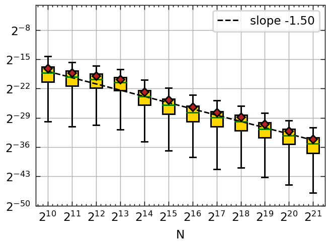
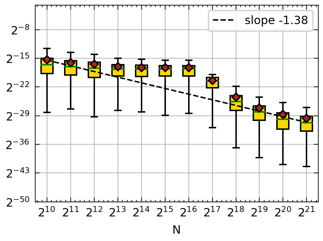
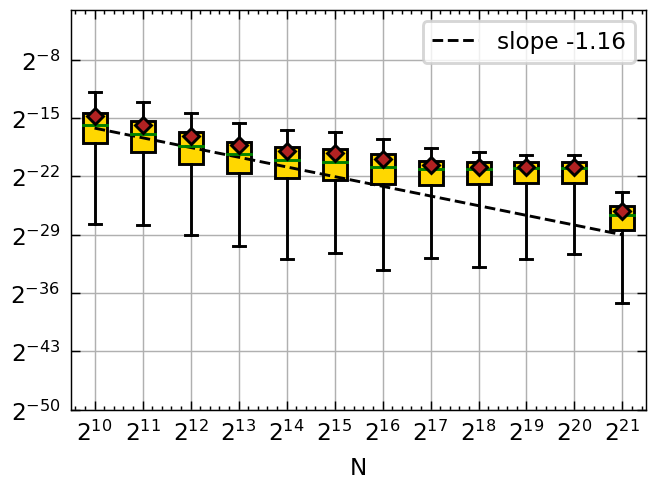
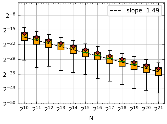
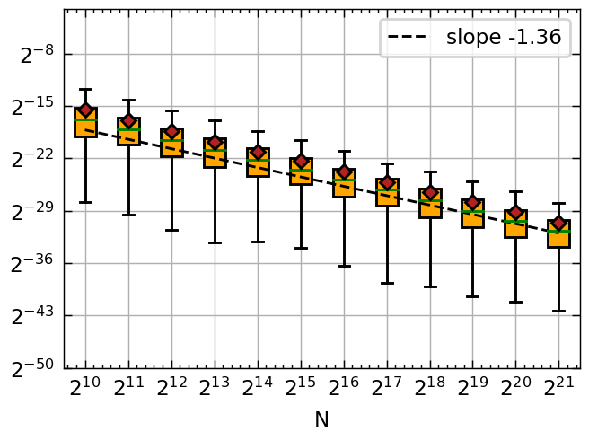
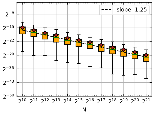
Figure 3: Ex1: The convergence of RQMC estimator variances. Top: RSLR; bottom: Sobol’ sequence. The columns from left to right correspond to $s=2,3,5$ respectively. $M=0.1$. Each boxplot displays the 1st to 99th percentile of 2,048 samples.

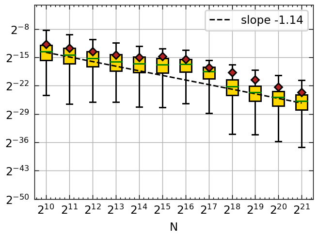
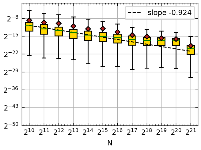
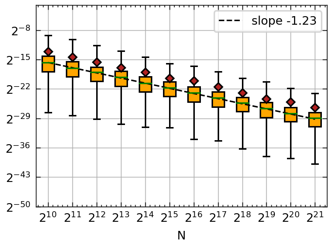
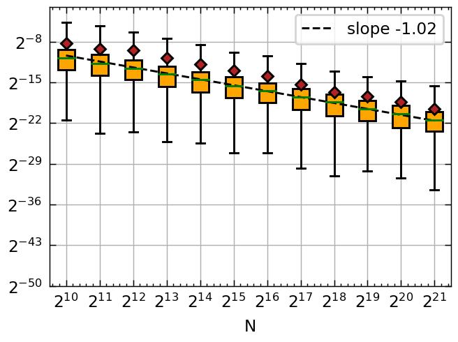
Figure 4: Ex1: The convergence of RQMC estimator variances. Top: RSLR; bottom: Sobol’ sequence. The columns from left to right correspond to $s=2,3,5$, respectively. $M=0.2$ when $s=2,3$, and $M=0.225$ when $s=5$. Each boxplot displays the 1st to 99th percentile of 2,048 samples.

From Figure 3, when $M=0.1$, both RSLR and the randomly scrambled Sobol’ sequence are affected by the hypersphere-type discontinuity rather than by the boundary growth conditions. For both sequences, the fitted convergence rates are close to $\mathcal{O}(N^{-1-\frac{1}{s}+\epsilon})$, faster than our theoretical results. When the value of $M$ is increased to $0.2$ for $s=2,3$ and $0.225$ for $s=5$ in Figure 4, the convergence rates are close to $\mathcal{O}(N^{-2+4M+\epsilon})$, suggesting the effects from the boundary growth condition, which is again faster than our theoretical results. The suboptimal observed rates for RSLR are due to the nonasymptotic regimes.

In Example 2, we consider the hyperplane-type discontinuity with $\Omega=\{\bm{t}\in[0,1]^{s}:\sum_{j=1}^{s}\bm{t}_{j}\leq 1\}$. The rest of the settings remain the same as in Example 1. The boxplots of squared errors are shown in Figure 5 and 6.

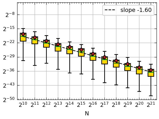
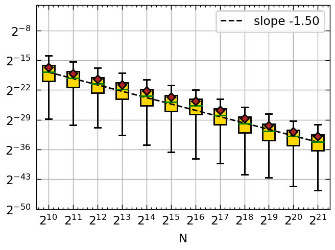
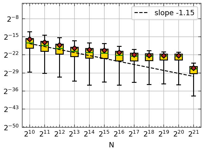
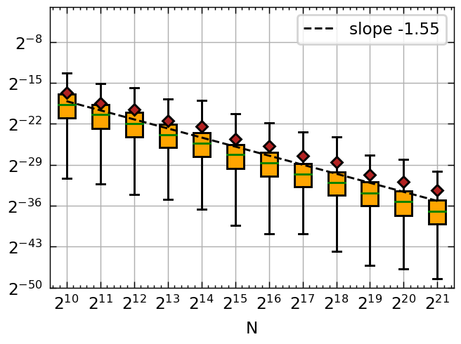
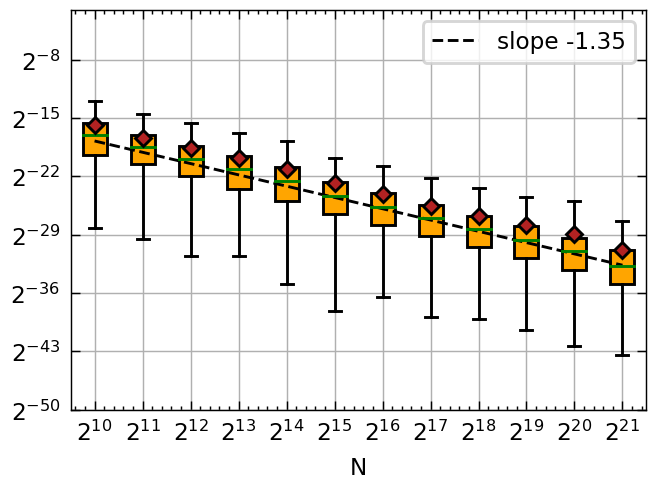
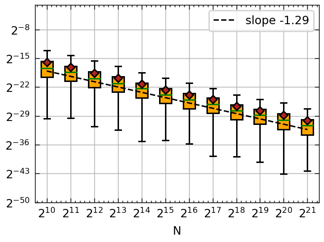
Figure 5: Ex2: The convergence of RQMC estimator variances. Top: RSLR; bottom: Sobol’ sequence. The columns from left to right correspond to $s=2,3,5$, respectively. $M=0.1$. Each boxplot displays the 1st to 99th percentile of 2,048 samples.

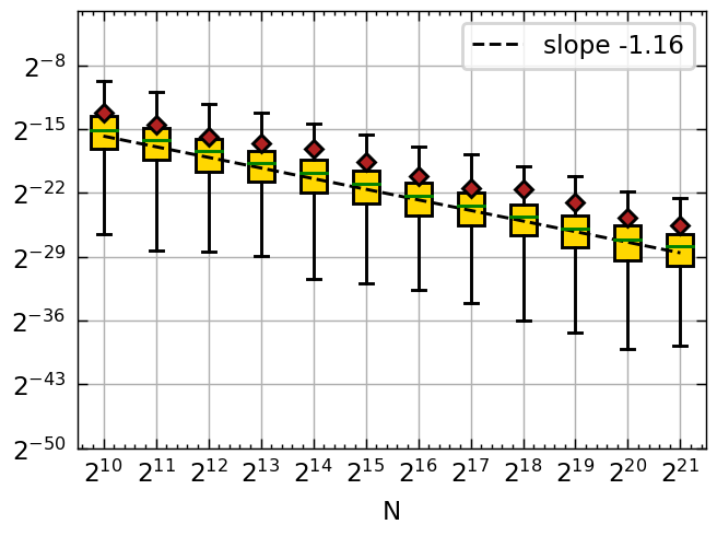
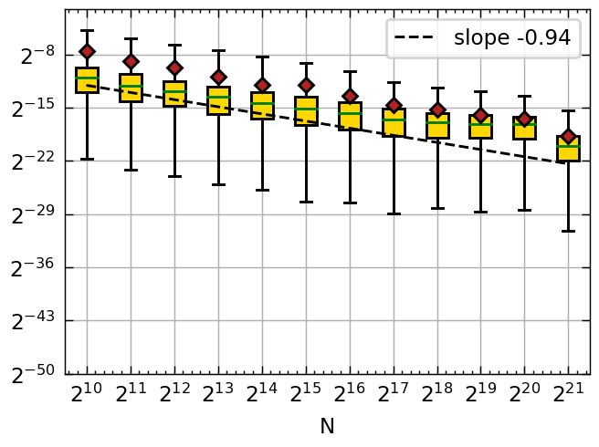
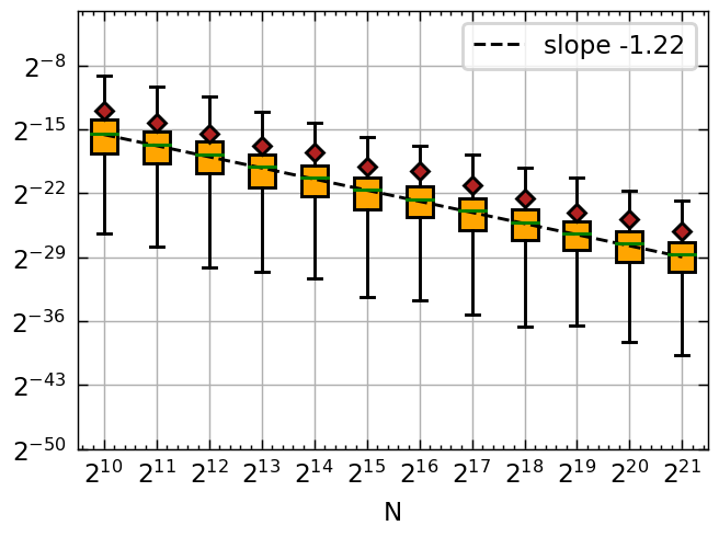
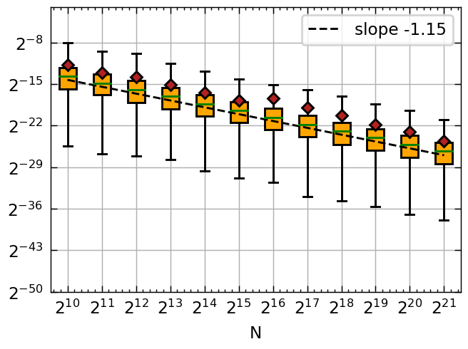
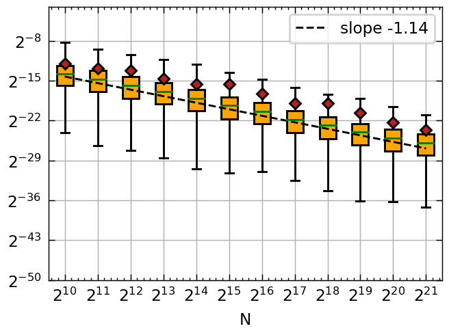
Figure 6: Ex2: The convergence of RQMC estimator variances. Top: RSLR; bottom: Sobol’ sequence. The columns from left to right correspond to $s=2,3,5$, respectively. $M=0.2$ when $s=2,3$, and $M=0.225$ when $s=5$. Each boxplot displays the 1st to 99th percentile of 2,048 samples.

The Sobol’ sequences behave similarly to those in Example 1 with the hypersphere-type discontinuity. It is worth discussing the RSLR. When $M=0.1$, in the case $s=2$, the fitted convergence $-1.60$ closely aligns with the convergence rate $\mathcal{O}(N^{-2+4M+\epsilon})$, suggesting the boundary growth condition, rather than the discontinuity, dominates the convergence rate — a contrast to Example 1. Moreover, when $s=3,5$, the fitted convergence rates are close to $\mathcal{O}(N^{-1-\frac{1}{s-1}+\epsilon})$, as if the dimension is reduced by 1 in the discontinuity effect. This difference from Example 1 stems from the different discontinuity boundaries. When $M$ are increased as in Figure 6, the boundary growth conditions dominate the convergence rates, which are similar to those in Example 1.

In Example 3, we consider an axis-parallel discontinuity. Specicially, we consider $\Omega=\{\bm{t}\in[0,1]^{s}:\min_{j=1}^{s}t_{j}\geq 1/2\}$ and set $M=0.1$. The boxplots of squared errors are shown in Figure 7.

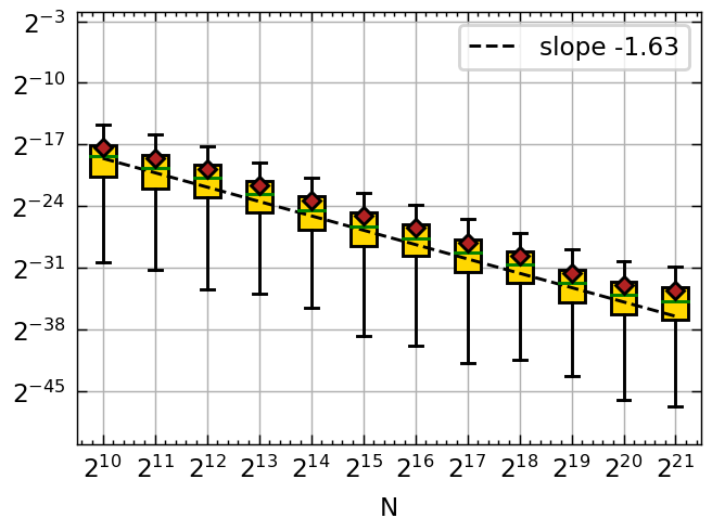
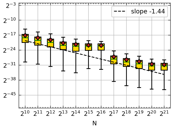
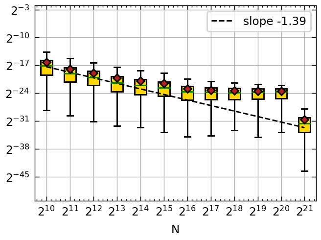
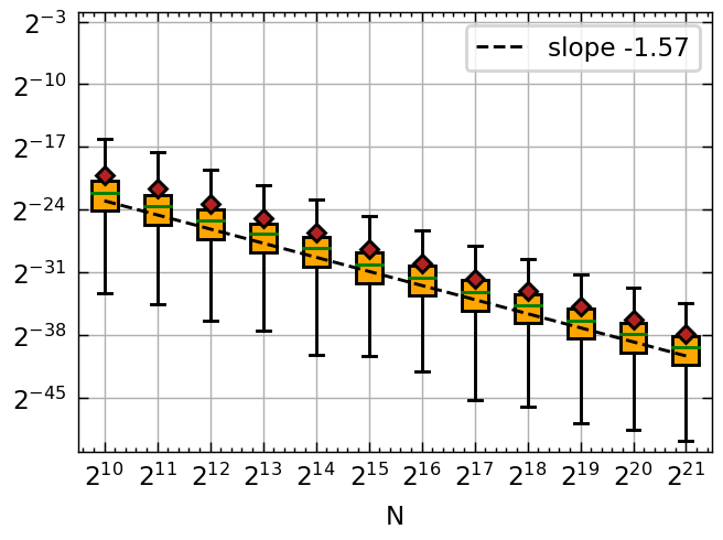
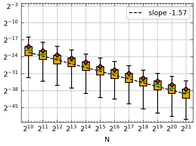
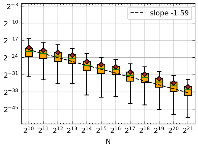
Figure 7: Ex3: The convergence of RQMC estimator variances. Top: RSLR, bottom: Sobol’ sequence. The columns from left to right correspond to $s=2,3,5$, respectively. $M=0.1$. Each boxplot displays the 1st to 99th percentile of 2,048 samples.

From Figure 7, the convergence rates of Sobol’ sequences for all three dimension settings closely align with our theoretical rates $\mathcal{O}(N^{-2+4M+\epsilon})$, indicating the boundary growth condition dominates the convergence rate. More nonasymptotic effects appear in the RSLR when dimension $s$ increases.

In Example 4, we consider a partial axis-parallel discontinuity. We consider $\Omega=\{\bm{t}\in[0,1]^{s}:\min_{j=1}^{2}\bm{t}_{j}\geq 1/2,\sum_{i=3}^{s}\bm{t}_{i}^{2}\geq 1\}$ with $M=0.1$ and dimensions $s=4,5,7$. The boxplots of squared errors are shown in Figure 8.

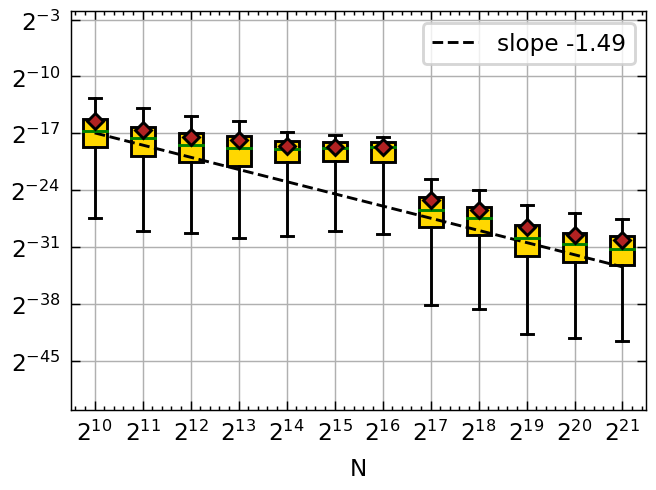
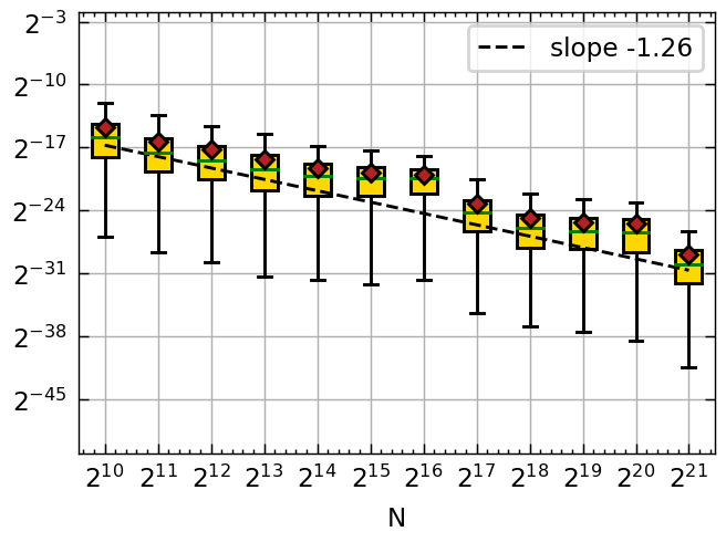
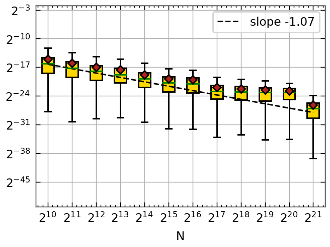
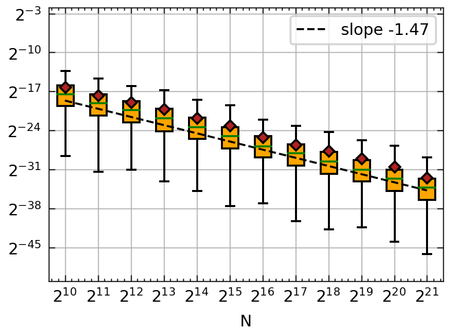
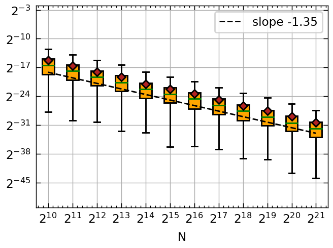
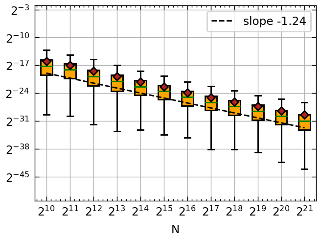
Figure 8: Ex4: The convergence of RQMC estimator variances. Top: RSLR, bottom: Sobol’ sequence. The columns from left to right corresponds to $s=4,5,7$, respectively. $M=0.1$. Each boxplot displays the 1st to 99th percentile of 2,048 samples.

The convergence rates from Figure 8 are similar to those in Figure 5 from Example 1. This indicates that in the case of partial axis-parallel discontinuity, the effects of the axis-parallel dimensions are marginal, which is consistent with our theoretical results.

6 Conclusions

This work presents a comparative study of the RSLR and the randomly scrambled Sobol’ sequences through spectral analysis. We analyze integrands whose Hardy–Krause variation is infinite, resulting from either the boundary unboundedness or interior discontinuities. We study sufficient conditions for these integrands and compare them to classical results. Owen’s boundary growth conditions bridge the gaps within integer orders of differentiability and convergence.

Both low-discrepancy sequences under consideration are insensitive to axis-parallel type discontinuities. For general discontinuous integrands with Sobol’ sequences, the convergence rates observed in the numerical results are faster than our theoretical results. One potential reason could be that the Hölder inequality applied in (97) does not provide optimal upper bounds. Another reason can be the loose upper bound in Lemma 4.6. Future work could aim to refine these upper bounds.

The effect of the discontinuity interface on the RSLR remains unclear. The work [8] studies the Fourier transform of indicator functions on $\mathbb{R}^{s}$ and reveals its dependency on the boundary curvature. Future work could extend the analysis in [8] to study the decay of Fourier coefficients, for instance, for the unbounded and discontinuous integrands examined in this work.

Furthermore, this study could facilitate the variance reduction techniques in the RQMC settings. For instance, in the context of importance sampling for QMC, as discussed in [11, 16], future efforts could consider the spectral properties to optimize the proposal distribution.

Appendix A Proof to Lemma 12

Proof A.1.

The variance of the RSLR estimator is given as

(104) $$\mathrm{Var}(I^{\mathrm{lat}}_{N})=\mathbb{E}[(I^{\mathrm{lat}}_{N})^{2}]-(\mathbb{E}[I^{\mathrm{lat}}_{N}])^{2}.$$

We continue the derivations as follows:

(105) $$\begin{split}(I^{\mathrm{lat}}_{N})^{2}&=\left(\sum_{\bm{n}\in\mathbb{Z}^{s}}\left({\hat{S}^{N}}_{\bm{n}}[\bm{t}+\bm{\Delta}]\right)^{*}c_{\bm{n}}\right)^{2}\\ &=\sum_{\bm{n},\bm{n}^{\prime}}c_{\bm{n}}^{*}{\hat{S}^{N}}_{\bm{n}}[\bm{t}+\bm{\Delta}]\left({\hat{S}^{N}}_{\bm{n}^{\prime}}[\bm{t}+\bm{\Delta}]\right)^{*}c_{\bm{n}^{\prime}}.\end{split}$$

Notice that in the case of RSLR, the spectral density is given by

(106) $$\begin{split}\hat{S}^{N}_{\bm{n}}[\bm{t}+\bm{\Delta}]&=e^{-i2\pi\bm{n}\cdot\bm{\Delta}}\frac{1}{N}\sum_{i=0}^{N-1}e^{-i2\pi\bm{n}\cdot\bm{t}_{i}}\\ &=e^{-i2\pi\bm{n}\cdot\bm{\Delta}}\hat{S}^{N}_{\bm{n}}[\bm{t}].\end{split}$$

With $\bm{\Delta}\sim\mathcal{U}([0,1]^{s})$, we have

(107) $$\begin{split}\mathbb{E}[\hat{S}^{N}_{\bm{n}}[\bm{t}+\bm{\Delta}]\hat{S}^{N}_{\bm{n}^{\prime}}[\bm{t}+\bm{\Delta}]]&=\mathbb{E}[e^{-i2\pi(\bm{n}-\bm{n}^{\prime})\cdot\bm{\Delta}}\hat{S}^{N}_{\bm{n}}[\bm{t}](\hat{S}^{N}_{\bm{n}^{\prime}}[\bm{t}])^{*}]\\ &=\mathbbm{1}_{\{\bm{n}=\bm{n}^{\prime}\}}\left\lvert\hat{S}^{N}_{\bm{n}}(\bm{t})\right\rvert^{2}.\end{split}$$

Thus we have,

(108) $$\mathbb{E}[(I^{\mathrm{lat}}_{N})^{2}]=\sum_{\bm{n}\in\mathbb{Z}^{s}}\left\lvert\hat{S}^{N}_{\bm{n}}[\bm{t}]\right\rvert^{2}\left\lvert c_{\bm{n}}\right\rvert^{2}$$

and

(109) $$\begin{split}\mathbb{E}[I^{\mathrm{lat}}_{N}]&={\mathbb{E}\mspace{-2.0mu}\left[\sum_{\bm{n}}\hat{S}^{N}_{\bm{n}}[\bm{t}+\bm{\Delta}]{c}^{*}_{\bm{n}}\right]}\\ &={\mathbb{E}\mspace{-2.0mu}\left[e^{-i2\pi\bm{n}\cdot\bm{\Delta}}\hat{S}^{N}_{\bm{n}}[\bm{t}]c^{*}_{\bm{n}}\right]}\\ &=\hat{S}^{N}_{0}[\bm{t}]c^{*}_{0}.\end{split}$$

(110) $$\mathbb{E}[I^{\mathrm{lat}}_{N}]^{2}=c_{0}(\hat{S}^{N}_{0}[\bm{t}])^{*}\hat{S}^{N}_{0}[\bm{t}]c^{*}_{0}={\left\lvert\hat{S}^{N}_{0}[\bm{t}]\right\rvert^{2}}\left\lvert c_{0}\right\rvert^{2}.$$

Appendix B Proof to Lemma 3.2

Proof B.1.

We compute $P_{\mathrm{lat}}(\bm{n})$ directly.

(111) $$\begin{split}P_{\mathrm{lat}}(\bm{n})&={\left\lvert\hat{S}^{N}_{\bm{n}}[\bm{t}]\right\rvert^{2}}\\ &=(\hat{S}^{N}_{\bm{n}}[\bm{t}])^{*}\hat{S}^{N}_{\bm{n}}[\bm{t}]\\ &=\frac{1}{N^{2}}\left(N+\sum_{i,j=0,i\neq j}^{N-1}e^{-i2\pi\bm{n}\cdot(\bm{t}_{i}-\bm{t}_{j})}\right)\\ &=\frac{1}{N^{2}}\left(N+\sum_{i,j=0,i<j}^{N-1}2\cos\left({2\pi\bm{n}\cdot(\bm{t}_{i}-\bm{t}_{j})}\right)\right).\end{split}$$

Recall that $\bm{t}_{i}=\frac{i}{N}\bm{z}\textrm{ mod }1$ and by using the periodicity, we have

(112) $$\sum_{i,j=0,i<j}^{N}2\cos\left({2\pi\bm{n}\cdot(\bm{t}_{i}-\bm{t}_{j})}\right)=\sum_{k=1}^{N-1}2(N-k)\cos\left({2\pi\bm{n}\cdot\left(\frac{k}{N}\bm{z}\right)}\right).$$

When $\bm{n}\cdot\bm{z}\equiv 0\mod N$, we have

(113) $$\sum_{i,j=0,i<j}^{N}2\cos\left({2\pi\bm{n}\cdot(\bm{t}_{i}-\bm{t}_{j})}\right)=N(N-1).$$

Otherwise let us denote

(114) $$Z_{N}\coloneqq\sum_{k=1}^{N-1}(N-k)e^{-i2\pi\bm{n}\cdot\left(\frac{k}{N}\bm{z}\right)}$$

and we are interested in $2Re(Z_{N})$. Let us first expand $Z_{N}$:

(115) $$\begin{split}Z_{N}&=\sum_{k=1}^{N-1}(N-k)e^{-i2\pi\bm{n}\cdot\left(\frac{k}{N}\bm{z}\right)}\\ &=\sum_{l=1}^{N-1}\sum_{k=1}^{l}e^{-i2\pi\bm{n}\cdot\left(\frac{k}{N}\bm{z}\right)}\\ &=\sum_{l=1}^{N-1}\frac{e^{i2\pi\frac{\bm{n}\cdot\bm{z}}{N}}-e^{i2\pi\frac{(l+1)\bm{n}\cdot\bm{z}}{N}}}{1-e^{i2\pi\frac{\bm{n}\cdot\bm{z}}{N}}}\\ &=(N-1)\frac{e^{i2\pi\frac{\bm{n}\cdot\bm{z}}{N}}}{1-e^{i2\pi\frac{\bm{n}\cdot\bm{z}}{N}}}-\frac{1}{1-e^{i2\pi\frac{\bm{n}\cdot\bm{z}}{N}}}\frac{e^{i2\pi\frac{2\bm{n}\cdot\bm{z}}{N}}-e^{i2\pi\frac{(N+1)\bm{n}\cdot\bm{z}}{N}}}{1-e^{i2\pi\frac{\bm{n}\cdot\bm{z}}{N}}}\\ &=(N-1)\frac{e^{i2\pi\frac{\bm{n}\cdot\bm{z}}{N}}-1}{2-2\cos(2\pi\frac{\bm{n}\cdot\bm{z}}{N})}-\frac{1-e^{-i2\pi\frac{\bm{n}\cdot\bm{z}}{N}}}{2-2\cos(2\pi\frac{\bm{n}\cdot\bm{z}}{N})}\cdot\frac{1-2e^{i2\pi\frac{\bm{n}\cdot\bm{z}}{N}}+e^{i2\pi\frac{2\bm{n}\cdot\bm{z}}{N}}}{2-2\cos(2\pi\frac{\bm{n}\cdot\bm{z}}{N})}\\ \end{split}$$

Now we compute $Re(Z_{N})$.

(116) $$\begin{split}Re(Z_{N})&=(N-1)\frac{\cos(i2\pi\frac{\bm{n}\cdot\bm{z}}{N})-1}{2-2\cos(2\pi\frac{\bm{n}\cdot\bm{z}}{N})}-\frac{3-4\cos(i2\pi\frac{\bm{n}\cdot\bm{z}}{N})+\cos(i2\pi\frac{2\bm{n}\cdot\bm{z}}{N})}{(2-2\cos(2\pi\frac{\bm{n}\cdot\bm{z}}{N}))^{2}}\\ &=-\frac{N-1}{2}-\frac{2-4\cos(i2\pi\frac{\bm{n}\cdot\bm{z}}{N})+2\cos^{2}(i2\pi\frac{\bm{n}\cdot\bm{z}}{N})}{(2-2\cos(2\pi\frac{\bm{n}\cdot\bm{z}}{N}))^{2}}\\ &=-\frac{N}{2}.\end{split}$$

Thus, we have

(117) $$\sum_{i,j=0,i<j}^{N-1}2\cos\left({2\pi\bm{n}\cdot(\bm{t}_{i}-\bm{t}_{j})}\right)=2Re(Z_{N})=-N,$$

and

(118) $${P_{\textrm{lat}}}(\bm{n})=\begin{cases}1,&\text{if}\ \bm{n}\cdot\bm{z}\equiv 0\mod N\\ 0,&\text{otherwise}.\end{cases}$$

Appendix C Proof to Lemma 3.7

Proof C.1.

In 1-D, the Fourier coefficients are given by

(119) $$\begin{split}c_{n}&=\int_{\mathbb{T}}f(t)e^{-i2\pi nt}dt\\ &=\int_{\mathbb{T}}f(t+\frac{1}{2n})e^{-i2\pi n(t+\frac{1}{2n})}dt\\ &=\int_{\mathbb{T}}-f(t+\frac{1}{2n})e^{-i2\pi nt}dt.\end{split}$$

Now we have two expressions for $c_{n}$, thus we have

(120) $$\begin{split}\lvert c_{n}\rvert&=\frac{1}{2}\left\lvert\int_{\mathbb{T}}f(t)e^{-i2\pi nt}dt+\int_{\mathbb{T}}-f(t+\frac{1}{2n})e^{-i2\pi nt}dt\right\rvert\\ &\leq\frac{1}{2}\int_{\mathbb{T}}\left\lvert f(t)-f(t+\frac{1}{2n})\right\rvert dt\\ &=\frac{1}{2}\int_{\mathbb{T}}\left\lvert\int_{[t,t+\frac{1}{2n}\textrm{ mod }1]}\frac{\partial f}{\partial t_{0}}dt_{0}\right\rvert dt\\ &\leq\frac{1}{2}\int_{\mathbb{T}}\left(\mathbbm{1}_{t\in[0,\frac{1}{2}-\frac{1}{2n})}\int_{t}^{t+\frac{1}{2n}}\left\lvert\frac{\partial f}{\partial t_{0}}\right\rvert dt_{0}+\mathbbm{1}_{t\in[\frac{1}{2}-\frac{1}{2n},1)}\int_{t+\frac{1}{2n}-1}^{t}\left\lvert\frac{\partial f}{\partial t_{0}}\right\rvert dt_{0}\right)dt.\end{split}$$

We will consider the following situations:(i) $t\in[0,\frac{1}{2}-\frac{1}{2n})$

(121) $$\begin{split}\int_{0}^{\frac{1}{2}-\frac{1}{2n}}\int_{t}^{t+\frac{1}{2n}}\left\lvert\frac{\partial f}{\partial t_{0}}\right\rvert dt_{0}dt&\leq\int_{0}^{\frac{1}{2}-\frac{1}{2n}}\int_{t}^{t+\frac{1}{2n}}t_{0}^{-A-1}dt_{0}dt\\ &=\frac{1}{A}\int_{0}^{\frac{1}{2}-\frac{1}{2n}}t^{-A}-\left(t+\frac{1}{2n}\right)^{-A}dt\\ &=\frac{1}{A(1-A)}\left[\left(\frac{1}{2}-\frac{1}{2n}\right)^{1-A}-2^{A-1}+\left(\frac{1}{2n}\right)^{1-A}\right].\end{split}$$

When (ii) $t\in[\frac{1}{2}-\frac{1}{2n},\frac{1}{2}]$, we have

(122) $$\int_{t}^{t+\frac{1}{2n}}\left\lvert\frac{\partial f}{\partial t_{0}}\right\rvert dt_{0}=\int_{t}^{\frac{1}{2}}\left\lvert\frac{\partial f}{\partial t_{0}}\right\rvert dt_{0}+\int_{\frac{1}{2}}^{t+\frac{1}{2n}}\left\lvert\frac{\partial f}{\partial t_{0}}\right\rvert dt_{0},$$

and

(123) $$\begin{split}\int_{\frac{1}{2}-\frac{1}{2n}}^{\frac{1}{2}}\int_{t}^{t+\frac{1}{2n}}\left\lvert\frac{\partial f}{\partial t_{0}}\right\rvert dt_{0}dt&=\int_{\frac{1}{2}-\frac{1}{2n}}^{\frac{1}{2}}\left(\int_{t}^{\frac{1}{2}}\left\lvert\frac{\partial f}{\partial t_{0}}\right\rvert dt_{0}+\int_{\frac{1}{2}}^{t+\frac{1}{2n}}\left\lvert\frac{\partial f}{\partial t_{0}}\right\rvert dt_{0}\right)dt\\ &\leq\frac{1}{A}\int_{\frac{1}{2}-\frac{1}{2n}}^{\frac{1}{2}}t^{-A}+(1-t-\frac{1}{2n})^{-A}-2\cdot\left(\frac{1}{2}\right)^{-A}dt\\ &=-\frac{1}{A}\cdot\frac{2^{A}}{n}+\frac{2}{A(1-A)}\left[2^{A-1}-2\cdot\left(\frac{1}{2}-\frac{1}{2n}\right)^{1-A}\right].\end{split}$$

Similar to case (i), when (iii) $t\in[\frac{1}{2},1-\frac{1}{2n})$, we have

(124) $$\int_{\frac{1}{2}}^{1-\frac{1}{2n}}\int_{t}^{t+\frac{1}{2n}}\left\lvert\frac{\partial f}{\partial t_{0}}\right\rvert dt_{0}dt\leq\frac{1}{A(1-A)}\left[\left(\frac{1}{2}-\frac{1}{2n}\right)^{1-A}-2^{A-1}+\left(\frac{1}{2n}\right)^{1-A}\right].$$

In case (iv) $t\in[1-\frac{1}{2n},1]$, we have

(125) $$\begin{split}\int_{1-\frac{1}{2n}}^{1}\left\lvert\int_{t}^{t+\frac{1}{2n}\textrm{ mod }1}\frac{\partial f}{\partial t_{0}}dt_{0}\right\rvert dt&\leq\int_{1-\frac{1}{2n}}^{1}\int_{t+\frac{1}{2n}-1}^{\frac{1}{2}}\left\lvert\frac{\partial f}{\partial t_{0}}\right\rvert dt_{0}+\int_{\frac{1}{2}}^{t}\left\lvert\frac{\partial f}{\partial t_{0}}\right\rvert dt_{0}dt\\ &\leq-\frac{1}{A}\cdot\frac{2^{A}}{2n}+\frac{2}{A(1-A)}\left(\frac{1}{2n}\right)^{1-A}.\end{split}$$

where in Equation (125) we have used the fact that $f$ is $1$-periodic. Thus, we have

(126) $$\lvert c_{n}\rvert\leq\frac{4}{A(1-A)}\left(\frac{1}{2n}\right)^{1-A}-\frac{2^{A+1}}{An}=\mathcal{O}(n^{-1+A}).$$

Similarly, in the case $A=0$, we will consider the following situations:(i) $t\in[0,\frac{1}{2}-\frac{1}{2n})$

(127) $$\begin{split}\int_{0}^{\frac{1}{2}-\frac{1}{2n}}\int_{t}^{t+\frac{1}{2n}}\left\lvert\frac{\partial f}{\partial t_{0}}\right\rvert dt_{0}dt&\leq\int_{0}^{\frac{1}{2}-\frac{1}{2n}}\int_{t}^{t+\frac{1}{2n}}t_{0}^{-1}dt_{0}dt\\ &=\int_{0}^{\frac{1}{2}-\frac{1}{2n}}\log\left(t+\frac{1}{2n}\right)-\log{t}dt\\ &=\frac{1}{2}\log{\frac{1}{2}}-\frac{1}{2}-\left(\frac{1}{2n}\log{\frac{1}{2n}}-\frac{1}{2n}\right)\\ &-\left(\frac{1}{2}-\frac{1}{2n}\right)\log{\left(\frac{1}{2}-\frac{1}{2n}\right)}+\frac{1}{2}-\frac{1}{2n}.\end{split}$$

In case (ii) when $t\in[\frac{1}{2}-\frac{1}{2n},\frac{1}{2})$, we have

(128) $$\begin{split}\int_{\frac{1}{2}-\frac{1}{2n}}^{\frac{1}{2}}\int_{t}^{t+\frac{1}{2n}}\left\lvert\frac{\partial f}{\partial t_{0}}\right\rvert dt_{0}dt&\leq\int_{\frac{1}{2}-\frac{1}{2n}}^{\frac{1}{2}}\int_{t}^{\frac{1}{2}}\left\lvert\frac{\partial f}{\partial t_{0}}\right\rvert dt_{0}+\int_{\frac{1}{2}}^{t+\frac{1}{2n}}\left\lvert\frac{\partial f}{\partial t_{0}}\right\rvert dt_{0}dt\\ &=\int_{\frac{1}{2}-\frac{1}{2n}}^{\frac{1}{2}}\log{\frac{1}{2}}-\log{t}dt+\log{\frac{1}{2}}-\log{\left(1-\frac{1}{2n}-t\right)}dt\\ &=\frac{1}{n}\log{\frac{1}{2}}-2\left[\frac{1}{2}\log{\frac{1}{2}}-\frac{1}{2}-\left(\frac{1}{2}-\frac{1}{2n}\right)\log{\left(\frac{1}{2}-\frac{1}{2n}\right)}+\frac{1}{2}-\frac{1}{2n}\right].\end{split}$$

The case (iii) when $t\in[\frac{1}{2},1-\frac{1}{2n})$ is similar to case (i), and we have

(129) $$\begin{split}\int_{0}^{\frac{1}{2}-\frac{1}{2n}}\int_{t}^{t+\frac{1}{2n}}\left\lvert\frac{\partial f}{\partial t_{0}}\right\rvert dt_{0}dt\leq&=\frac{1}{2}\log{\frac{1}{2}}-\frac{1}{2}-\left(\frac{1}{2n}\log{\frac{1}{2n}}-\frac{1}{2n}\right)\\ &-\left(\frac{1}{2}-\frac{1}{2n}\right)\log{\left(\frac{1}{2}-\frac{1}{2n}\right)}+\frac{1}{2}-\frac{1}{2n}.\end{split}$$

In case (iv) when $t\in[1-\frac{1}{2n},1]$, we have

(130) $$\begin{split}\int_{1-\frac{1}{2n}}^{1}\int_{t+\frac{1}{2n}-1}^{t}\left\lvert\frac{\partial f}{\partial t_{0}}\right\rvert dt_{0}dt&\leq\int_{1-\frac{1}{2n}}^{1}\int_{t+\frac{1}{2n}-1}^{\frac{1}{2}}\left\lvert\frac{\partial f}{\partial t_{0}}\right\rvert dt_{0}+\int_{\frac{1}{2}}^{t}\left\lvert\frac{\partial f}{\partial t_{0}}\right\rvert dt_{0}dt\\ &=\int_{1-\frac{1}{2n}}^{1}2\log{\frac{1}{2}}-\log{\left(1-t\right)}dt-\log{\left(t+\frac{1}{2n}-1\right)}dt\\ &=\frac{1}{n}\log{\frac{1}{2}}.\end{split}$$

Thus we have in case $A=0$,

(131) $$\lvert c_{n}\rvert=-\left(\frac{1}{n}\log{\frac{1}{2n}}-\frac{1}{n}\right)+\frac{2}{n}\log{\frac{1}{2}}=\mathcal{O}(n^{-1}\log n).$$

Appendix D Proof to Lemma 3.12

Proof D.1.

For $\bm{t}\in[0,1)^{s}$ and $\bm{n}\in\mathbb{N}^{s}$, we will consider a nonempty set $\mathfrak{u}\subseteq 1:s$ such that $\bm{n}_{\mathfrak{u}}=\bm{n}^{\mathfrak{u}}:0^{-\mathfrak{u}}$. Without loss of generality, we assume that ${1}\in\mathfrak{u}$. We split the domain $[0,1]^{s}$ into two parts depending on whether the interval $[\bm{t},\bm{t}+\frac{1}{2\bm{n}_{\mathfrak{u}}}]$ intersects with the boundary of $\Omega$. We first consider the situation when $[\bm{t},\bm{t}+\frac{1}{2\bm{n}_{\mathfrak{u}}}]\cap\partial\Omega\neq\emptyset$.

We proceed with a proof by induction. For a function $f=\mathbbm{1}_{\Omega}\cdot g$, with $g$ satisfying the boundary growth condition (2.4) with $0<A_{j}<1/2$ for $j=1,\dotsc,s$ and axis-parallel $\Omega=[\bm{a},\bm{b}]\subseteq[0,1]^{s}$, we assume

(132) $$\int_{[0,1]^{s}}\mathbbm{1}_{[\bm{t},\bm{t}+\frac{1}{2\bm{n}_{\mathfrak{u}}})\cap\partial\Omega\neq\emptyset}\left\lvert\Delta(f;\bm{t},\bm{t}+\frac{1}{2\bm{n}_{\mathfrak{u}}})\right\rvert d\bm{t}\lesssim\prod_{j=1}^{s}\bm{n}_{j}^{\max(-1+A_{j},-1)}.$$

The case $s=1$ is already proved in Lemma 3.7. We assume the statement holds for $s-1$ dimensions. Now in the case of $s$ dimensions, we can split the dimensions into $1$ and $2:s$.

(133) $$\begin{split}\lvert c_{\bm{n}}\rvert&\leq\frac{1}{2^{s}}\int_{[0,1]^{s}}\mathbbm{1}_{[\bm{t},\bm{t}+\frac{1}{2\bm{n}_{\mathfrak{u}}}]\cap\partial\Omega\neq\emptyset}\left\lvert\Delta(f;\bm{t},\bm{t}+\frac{1}{2\bm{n}_{\mathfrak{u}}})\right\rvert d\bm{t}\\ &=\frac{1}{2^{s}}\int_{[0,1]^{s-1}}\int_{0}^{1}\mathbbm{1}_{[\bm{t},\bm{t}+\frac{1}{2\bm{n}_{\mathfrak{u}}}]\cap\partial\Omega\neq\emptyset}\left\lvert\Delta(f;\bm{t},\bm{t}+\frac{1}{2\bm{n}_{\mathfrak{u}}})\right\rvert d\bm{t}_{1}d\bm{t}_{-1}\\ &=\frac{1}{2^{s}}\int_{[0,1]^{s-1}}\left(\mathbbm{1}_{[\bm{t}_{-1},\bm{t}_{-1}+\frac{1}{2\bm{n}_{\mathfrak{u}-1}}]\cap\partial\Omega=\emptyset}\int_{0}^{1}\mathbbm{1}_{[\bm{t}_{1},\bm{t}_{1}+\frac{1}{2\bm{n}_{1}}]\cap\partial\Omega\neq\emptyset}\left\lvert\Delta(f;\bm{t},\bm{t}+\frac{1}{2\bm{n}_{\mathfrak{u}}})\right\rvert d\bm{t}_{1}\right.\\ &\left.\quad\quad\quad+\mathbbm{1}_{[\bm{t}_{-1},\bm{t}_{-1}+\frac{1}{2\bm{n}_{\mathfrak{u}-1}}]\cap\partial\Omega\neq\emptyset}\int_{0}^{1}\left\lvert\Delta(f;\bm{t},\bm{t}+\frac{1}{2\bm{n}_{\mathfrak{u}}})\right\rvert d\bm{t}_{1}\right)d\bm{t}_{-1}.\end{split}$$

In the following, we will consider two situations with the dimensions $2:s$. First, when $[\bm{t}_{-1},\bm{t}_{-1}+\frac{1}{2\bm{n}_{\mathfrak{u}-1}})\cap\partial\Omega=\emptyset$ and $[\bm{t}_{1},\bm{t}_{1}+\frac{1}{2\bm{n}_{1}}]\cap\partial\Omega\neq\emptyset$ we have the triangular inequality

(134) $$\lvert\Delta(f;\bm{t},\bm{t}+\frac{1}{2\bm{n}_{\mathfrak{u}}})\rvert\leq\sum_{\mathfrak{v}\subseteq\mathfrak{u}}\prod_{j\in\mathfrak{u}}\phi\left(\left(\bm{t}^{\mathfrak{v}}:(\bm{t}+\frac{1}{2\bm{n}_{\mathfrak{u}}})^{\mathfrak{u}-\mathfrak{v}}\right)_{j}\right)^{-A_{j}}$$

Notice that we have the following decomposition in the direction of $\bm{t}_{1}$ of the alternating sum,

(135) $$\left\lvert\Delta(f;\bm{t},\bm{t}+\frac{1}{2\bm{n}_{\mathfrak{u}}})\right\rvert\\ =\left\lvert\sum_{\mathfrak{v}\subseteq\mathfrak{u}-1}(-1)^{\lvert\mathfrak{v}\rvert}f(\bm{t}^{\mathfrak{v}}:(\bm{t}+\frac{1}{2\bm{n}_{\mathfrak{u}}})^{\mathfrak{u}-\mathfrak{v}})-(-1)^{\lvert\mathfrak{v}\rvert}f(\bm{t}^{\mathfrak{v}+1}:(\bm{t}+\frac{1}{2\bm{n}_{\mathfrak{u}}})^{\mathfrak{u}-(\mathfrak{v}+1)})\right\rvert$$

and we proceed the first part of Equation (133) as

(136) $$\begin{split}&\int_{[0,1]^{s-1}}\mathbbm{1}_{[\bm{t}_{-1},\bm{t}_{-1}+\frac{1}{2\bm{n}_{\mathfrak{u}-1}}]\cap\partial\Omega=\emptyset}\int_{\bm{a}_{1}\in[\bm{t}_{1},\bm{t}_{1}+\frac{1}{2\bm{n}_{1}}]\cup\bm{b}_{1}\in[\bm{t}_{1},\bm{t}_{1}+\frac{1}{2\bm{n}_{1}}]}\left\lvert\Delta(f;\bm{t},\bm{t}+\frac{1}{2\bm{n}_{\mathfrak{u}}})\right\rvert d\bm{t}_{1}d\bm{t}_{-1}\\ &=\int_{[0,1]^{s-1}}\mathbbm{1}_{[\bm{t}_{-1},\bm{t}_{-1}+\frac{1}{2\bm{n}_{\mathfrak{u}-1}}]\cap\partial\Omega=\emptyset}\\ &\quad\quad\int_{[\bm{a}_{1},\bm{a}_{1}+\frac{1}{2\bm{n}_{1}}]\cup[\bm{b}_{1}-\frac{1}{2\bm{n}_{1}},\bm{b}_{1}]}\left\lvert\sum_{\mathfrak{v}\subseteq\mathfrak{u}-1}(-1)^{\lvert\mathfrak{v}\rvert}f\left(\bm{t}^{\mathfrak{v}+1}:(\bm{t}+\frac{1}{2\bm{n}_{\mathfrak{u}}})^{-(\mathfrak{v}+1)}\right)\right\rvert d\bm{t}_{1}d\bm{t}_{-1}\\ &=\int_{[0,1]^{s-1}}\mathbbm{1}_{[\bm{t}_{-1},\bm{t}_{-1}+\frac{1}{2\bm{n}_{\mathfrak{u}-1}}]\cap\partial\Omega=\emptyset}\int_{[\bm{a}_{1},\bm{a}_{1}+\frac{1}{2\bm{n}_{1}}]\cup[\bm{b}_{1}-\frac{1}{2\bm{n}_{1}},\bm{b}_{1}]}\\ &\quad\quad\left\lvert\int_{[\bm{t}_{\mathfrak{u}-1},\bm{t}_{\mathfrak{u}-1}+\frac{1}{2\bm{n}_{\mathfrak{u}-1}}\textrm{ mod }1]}\partial^{\mathfrak{u}-1}f(\bm{\tau}\mid\bm{\tau_{1}}=\bm{t}_{1})d\bm{\tau}_{\mathfrak{u}-1}\right\rvert d\bm{t}_{1}d\bm{t}_{-1}\\ &\leq\int_{[0,1]^{s-1}}\mathbbm{1}_{[\bm{t}_{-1},\bm{t}_{-1}+\frac{1}{2\bm{n}_{\mathfrak{u}-1}}]\cap\partial\Omega=\emptyset}\int_{[\bm{a}_{1},\bm{a}_{1}+\frac{1}{2\bm{n}_{1}}]\cup[\bm{b}_{1}-\frac{1}{2\bm{n}_{1}},\bm{b}_{1}]}\\ &\quad\quad\int_{[\bm{t}_{\mathfrak{u}-1},\bm{t}_{\mathfrak{u}-1}+\frac{1}{2\bm{n}_{\mathfrak{u}-1}}\textrm{ mod }1]}\left\lvert\partial^{\mathfrak{u}-1}f(\bm{\tau}\mid\bm{\tau_{1}}=\bm{t}_{1})\right\rvert d\bm{\tau}_{\mathfrak{u}-1}d\bm{t}_{1}d\bm{t}_{-1}\\ &\leq\int_{[0,1]^{s-1}}\mathbbm{1}_{[\bm{t}_{-1},\bm{t}_{-1}+\frac{1}{2\bm{n}_{\mathfrak{u}-1}}]\cap\partial\Omega=\emptyset}\int_{[\bm{a}_{1},\bm{a}_{1}+\frac{1}{2\bm{n}_{1}}]\cup[\bm{b}_{1}-\frac{1}{2\bm{n}_{1}},\bm{b}_{1}]}\\ &\quad\quad\int_{[\bm{t}_{\mathfrak{u}-1},\bm{t}_{\mathfrak{u}-1}+\frac{1}{2\bm{n}_{\mathfrak{u}-1}}\textrm{ mod }1]}\phi(\bm{t}_{1})^{-A_{1}}\prod_{j\in\mathfrak{u}-1}\phi(\bm{\tau}_{j})^{-1-A_{j}}d\bm{\tau}_{\mathfrak{u}-1}d\bm{t}_{1}d\bm{t}_{-1}\\ &\leq\int_{[\bm{a}_{1},\bm{a}_{1}+\frac{1}{2\bm{n}_{1}}]\cup[\bm{b}_{1}-\frac{1}{2\bm{n}_{1}},\bm{b}_{1}]}\phi(\bm{t}_{1})^{-A_{1}}d\bm{t}_{1}\\ &\quad\quad\cdot\int_{[0,1]^{s-1}}\int_{[\bm{t}_{-1},\bm{t}_{-1}+\frac{1}{2\bm{n}_{\mathfrak{u}-1}}\textrm{ mod }1]}\prod_{j\in\mathfrak{u}-1}\phi(\bm{\tau}_{j})^{-1-A_{j}}d\bm{\tau}_{\mathfrak{u}-1}d\bm{t}_{-1}\\ &\leq\prod_{j\in\mathfrak{u}}\bm{n}_{j}^{-1+A_{j}}\end{split}$$

where in the second line we have considered the support of $f$, such that either $\sum_{\mathfrak{v}\subseteq\mathfrak{u}-1}(-1)^{\lvert\mathfrak{v}\rvert}f(\bm{t}^{\mathfrak{v}+1}:(\bm{t}+\frac{1}{2\bm{n}_{\mathfrak{u}}})^{-(\mathfrak{v}+1)})$ or $\sum_{\mathfrak{v}\subseteq\mathfrak{u}-1}(-1)^{\lvert\mathfrak{v}\rvert}f(\bm{t}^{\mathfrak{v}}:(\bm{t}+\frac{1}{2\bm{n}_{\mathfrak{u}}})^{-\mathfrak{v}})$ is zero, and the last line can be refered to the proof in Appendix C. Next, when $[\bm{t}_{-1},\bm{t}_{-1}+\frac{1}{2\bm{n}_{\mathfrak{u}-1}})\cap\partial\Omega\neq\emptyset$, we will further consider two situations of the dimension 1, namely, $\bm{a}_{1}\in[\bm{t}_{1},\bm{t}_{1}+\frac{1}{2\bm{n}_{1}}]\cup\bm{b}_{1}\in[\bm{t}_{1},\bm{t}_{1}+\frac{1}{2\bm{n}_{1}}]$ and $\bm{a}_{1}\notin[\bm{t}_{1},\bm{t}_{1}+\frac{1}{2\bm{n}_{1}}]\cap\bm{b}_{1}\notin[\bm{t}_{1},\bm{t}_{1}+\frac{1}{2\bm{n}_{1}}]$. When $\bm{a}_{1}\in[\bm{t}_{1},\bm{t}_{1}+\frac{1}{2\bm{n}_{1}}]\cup\bm{b}_{1}\in[\bm{t}_{1},\bm{t}_{1}+\frac{1}{2\bm{n}_{1}}]$,

(137) $$\begin{split}&\int_{\bm{a}_{1}\in[\bm{t}_{1},\bm{t}_{1}+\frac{1}{2\bm{n}_{1}}]\cup\bm{b}_{1}\in[\bm{t}_{1},\bm{t}_{1}+\frac{1}{2\bm{n}_{1}}]}\\ &\left\lvert\sum_{\mathfrak{v}\subseteq\mathfrak{u}-1}(-1)^{\lvert\mathfrak{v}\rvert}f(\bm{t}^{\mathfrak{v}}:(\bm{t}+\frac{1}{2\bm{n}_{\mathfrak{u}}})^{\mathfrak{u}-\mathfrak{v}})-(-1)^{\lvert\mathfrak{v}\rvert}f(\bm{t}^{\mathfrak{v}+1}:(\bm{t}+\frac{1}{2\bm{n}_{\mathfrak{u}}})^{\mathfrak{u}-(\mathfrak{v}+1)})\right\rvert d\bm{t}_{1}\\ &=\int_{[\bm{a}_{1},\bm{a}_{1}+\frac{1}{2\bm{n}_{1}})\vee[\bm{b}_{1}-\frac{1}{2\bm{n}_{1}},\bm{b}_{1})}\left\lvert\sum_{\mathfrak{v}\subseteq\mathfrak{u}-1}(-1)^{\lvert\mathfrak{v}\rvert}f\left(\bm{t}^{\mathfrak{v}+1}:(\bm{t}+\frac{1}{2\bm{n}_{\mathfrak{u}}})^{-(\mathfrak{v}+1)}\right)\right\rvert d\bm{t}_{1}.\end{split}$$

The function $f(\bm{t}_{-1}\mid\bm{t}_{1})$ satisfy the boundary growth condition, i.e.,

(138) $$\left\lvert\partial^{\mathfrak{v}}f(\bm{t}_{-1}\mid\bm{t}_{1})\right\rvert\leq\prod_{j\in\mathfrak{v}}\phi(\bm{t}_{j})^{-A_{j}}\prod_{k\in-\mathfrak{v}}\phi(\bm{t}_{k})^{-A_{k}}$$

for $\mathfrak{v}\subseteq\mathfrak{u}-1$. By our assumption, we have

(139) $$\begin{split}&\int_{[0,1]^{s-1}}\mathbbm{1}_{[\bm{t}_{-1},\bm{t}_{-1}+\frac{1}{2\bm{n}_{\mathfrak{u}-1}})\cap\partial\Omega\neq\emptyset}\left\lvert\sum_{\mathfrak{v}\subseteq\mathfrak{u}-1}(-1)^{\lvert\mathfrak{v}\rvert}f\left(\bm{t}^{\mathfrak{v}+1}:(\bm{t}+\frac{1}{2\bm{n}_{\mathfrak{u}}})^{-(\mathfrak{v}+1)}\right)\right\rvert d\bm{t}_{-1}\\ &\leq\phi(\bm{t}_{1})^{-A_{j}}\prod_{j\in\mathfrak{u}-1}\bm{n}_{j}^{-1+A_{j}}.\end{split}$$

Notice that

(140) $$\int_{[\bm{a}_{1},\bm{a}_{1}+\frac{1}{2\bm{n}_{1}})\cup[\bm{b}_{1}-\frac{1}{2\bm{n}_{1}},\bm{b}_{1})}\phi(\bm{t}_{1})^{-A_{1}}d\bm{t}_{1}\lesssim\bm{n}_{1}^{-1+A_{1}}.$$

When $\bm{a}_{1}\notin[\bm{t}_{1},\bm{t}_{1}+\frac{1}{2\bm{n}_{1}}]\cap\bm{b}_{1}\notin[\bm{t}_{1},\bm{t}_{1}+\frac{1}{2\bm{n}_{1}}]$

(141) $$\begin{split}&\int_{\bm{a}_{1}\notin[\bm{t}_{1},\bm{t}_{1}+\frac{1}{2\bm{n}_{1}}]\cap\bm{b}_{1}\notin[\bm{t}_{1},\bm{t}_{1}+\frac{1}{2\bm{n}_{1}}]}\\ &\left\lvert\sum_{\mathfrak{v}\subseteq\mathfrak{u}-1}(-1)^{\lvert\mathfrak{v}\rvert}f\left(\bm{t}^{\mathfrak{v}}:(\bm{t}+\frac{1}{2\bm{n}_{\mathfrak{u}}})^{-\mathfrak{v}}\right)-(-1)^{\lvert\mathfrak{v}\rvert}f\left(\bm{t}^{\mathfrak{v}+1}:(\bm{t}+\frac{1}{2\bm{n}_{\mathfrak{u}}})^{-(\mathfrak{v}+1)}\right)\right\rvert d\bm{t}_{1}\\ &\leq\int_{0}^{1}\int_{[\bm{t}_{1},\bm{t}_{1}+\frac{1}{2\bm{n}_{1}}\textrm{ mod }1]}\left\lvert\sum_{\mathfrak{v}\subseteq\mathfrak{u}-1}(-1)^{\lvert\mathfrak{v}\rvert}\partial^{1}f(\bm{\tau}\mid\bm{\tau}_{\mathfrak{u}-1}=\bm{t}^{\mathfrak{v}}:(\bm{t}+\frac{1}{2\bm{n}_{\mathfrak{u}}})^{\mathfrak{u}-1-\mathfrak{v}})\right\rvert d\bm{\tau}_{1}d\bm{t}_{1}\\ \end{split}$$

Notice that $\partial^{1}f(\bm{t}_{-1}\mid\bm{t}_{1})$ satisfy the boundary growth condition. By our assumption, we have

(142) $$\begin{split}&\int_{[0,1]^{s-1}}\mathbbm{1}_{[\bm{t}_{-1},\bm{t}_{-1}+\frac{1}{2\bm{n}_{\mathfrak{u}-1}})\cap\partial\Omega\neq\emptyset}\\ &\quad\quad\left\lvert\sum_{\mathfrak{v}\subseteq\mathfrak{u}-1}(-1)^{\lvert\mathfrak{v}\rvert}\partial^{1}f(\bm{\tau}\mid\bm{\tau}_{\mathfrak{u}-1}=\bm{t}^{\mathfrak{v}}:(\bm{t}+\frac{1}{2\bm{n}_{\mathfrak{u}}})^{\mathfrak{u}-1-\mathfrak{v}})\right\rvert d\bm{t}_{-1}\\ &\leq\phi(\bm{t}_{1})^{-1-A_{j}}\prod_{j\in\mathfrak{u}-1}\bm{n}_{j}^{-1+A_{j}}.\end{split}$$

Notice that

(143) $$\int_{0}^{1}\int_{[\bm{t},\bm{t}+\frac{1}{2\bm{n}_{1}}\textrm{ mod }1]}\phi(\bm{\tau}_{1})^{-1-A_{1}}d\bm{\tau}_{1}d\bm{t}_{1}\lesssim\bm{n}_{1}^{-1+A_{1}}.$$

Combining (136), (139), (140), (142), (143) the result follows.

Appendix E Walsh functions

Walsh (1923) introduced a system of functions denoted by ${}_{b}{\mathrm{wal}}_{k}$.

Definition E.1 (Walsh functions in 1d).

Let $k\in\mathbb{N}_{0}$ with $b$-adic expansion $k=\kappa_{0}+\kappa_{1}b+\kappa_{2}b^{2}+\cdots$. For $b\geq 2$ we denote by $\omega_{b}$ the primitive $b$th root of unity $\omega_{b}=e^{2\pi i/b}$. Then the $b$-ary Walsh function ${}_{b}{\mathrm{wal}}_{k}$ is defined by

$${}_{b}{\mathrm{wal}}_{k}(x)=\omega_{b}^{\kappa_{0}\xi_{1}+\kappa_{1}\xi_{2}+\cdots}$$

for $x\in[0,1)$ with $b$-adic expansion $x=\xi_{1}b^{-1}+\xi_{2}b^{-2}+\cdots$ (unique in the sense that infinitely many of the digits $\xi_{i}$ must be different from $b-1$).

In the following we present the proof to Lemma 49.

Proof E.2.

For $\bm{k}=(\bm{k}_{1},\dotsc,\bm{k}_{s})$, the $s$-dimensional Walsh-Dirichlet kernel is given by

(144) $$\begin{split}D_{\bm{\ell}}(\bm{z})&=\sum_{\bm{k}_{1}=0}^{b^{\bm{\ell}_{1}}-1}\cdots\sum_{\bm{k}_{s}=0}^{b^{\bm{\ell}_{s}}-1}{}_{b}{\mathrm{wal}}_{\bm{k}}(\bm{z})\\ &=\sum_{\bm{k}_{1}=0}^{b^{\bm{\ell}_{1}}-1}\cdots\sum_{\bm{k}_{s}=0}^{b^{\bm{\ell}_{s}}-1}\prod_{j=1}^{s}{}_{b}{\mathrm{wal}}_{\bm{k}_{j}}(\bm{z}_{j})\\ &=\prod_{j=1}^{s}b^{\bm{\ell}_{j}}\mathbbm{1}_{\bm{z}_{j}\in[0,b^{-\bm{\ell}_{j}})}\\ &=\mathbbm{1}_{\bm{z}\in[0,b^{-\bm{\ell}})}\prod_{j=1}^{s}b^{\bm{\ell}_{j}}.\end{split}$$

Notice that the Walsh–Fourier coefficient is given by

(145) $$\bar{f}(\bm{k})=\int_{[0,1]^{s}}f(\bm{t})\left({}_{b}{\mathrm{wal}}_{\bm{k}}(\bm{t})\right)^{*}d\bm{t}.$$

Substitute (145) into (49), we have

(146) $$\begin{split}\sum_{\bm{k}\in T_{\bm{\ell}}}\bar{f}(\bm{k}){}_{2}{\mathrm{wal}}_{\bm{k}}(\bm{t})&=\sum_{\bm{k}\in T_{\bm{\ell}}}\int_{[0,1]^{s}}f(\bm{y})\left({}_{2}{\mathrm{wal}}_{\bm{k}}(\bm{y})\right)^{*}{}_{2}{\mathrm{wal}}_{\bm{k}}(\bm{t})d\bm{y}\\ &=\sum_{\bm{k}\in T_{\bm{\ell}}}\int_{[0,1]^{s}}f(\bm{y}){}_{2}{\mathrm{wal}}_{\bm{k}}(\bm{y}\ominus\bm{t})d\bm{y}\\ &=\int_{[0,1]^{s}}f(\bm{y})\sum_{\bm{k}\in T_{\bm{\ell}}}{}_{2}{\mathrm{wal}}_{\bm{k}}(\bm{y}\ominus\bm{t})d\bm{y}\end{split}$$

where $\ominus$ denotes the digit-wise subtraction modulo $2$. Refering to (144), the Walsh–Dirichlet kernel $\sum_{\bm{k}\in T_{\bm{\ell}}}{}_{2}{\mathrm{wal}}_{\bm{k}}(\bm{y}\ominus\bm{t})$ is nonzero when $\bm{y}\ominus\bm{t}\in[0,2^{-\bm{\ell}}]$. In this case, the first $\bm{\ell}_{j}$ digits of $\bm{y}_{j}$ and $\bm{t}_{j}$ must match for all $j=1,\dotsc,s$, which is equivalent to the condition $\left\lfloor\bm{y}_{j}2^{\bm{\ell}_{j}}\right\rfloor=\left\lfloor\bm{t}_{j}2^{\bm{\ell}_{j}}\right\rfloor$ for $j=1,\dotsc,s$. Thus we have

(147) $$\sum_{\bm{k}\in T_{\bm{\ell}}}\bar{f}(\bm{k}){}_{2}{\mathrm{wal}}_{\bm{k}}(\bm{t})=\prod_{j=1}^{s}2^{\bm{\ell}_{j}}\int_{\cap_{j=1}^{s}\left\lfloor\bm{y}_{j}2^{\bm{\ell}_{j}}\right\rfloor=\left\lfloor\bm{t}_{j}2^{\bm{\ell}_{j}}\right\rfloor}f(\bm{y})d\bm{y}.$$

Appendix F Proof of Lemma 4.5

Proof F.1.

Following [10], we consider a partition of $[0,1]^{s}$ with the elementary intervals $E_{\bm{\ell},\bm{k}}$ with $b=2$, $\bm{\ell}\in\mathbb{N}_{0}^{s}$, as defined in (2). Similar to Equation (74), we define $\bar{\bm{\ell}}\coloneqq\max(\bm{\ell}-1,0)$, $\bar{\bm{\ell}}_{\mathfrak{u}}\coloneqq{\bm{\ell}}_{\mathfrak{u}}-1$ and $f(\bm{y})\coloneqq 0$ when $\bm{y}\notin[0,1]^{s}$ for the notation simplicity. We have,

(148) $$\sigma^{2}_{\bm{\ell}}(f)=\sum_{\begin{subarray}{c}\bm{k}\in\mathbb{N}_{0}^{s}\\ {\bm{k}\leq 2^{\bar{\bm{\ell}}}-1}\end{subarray}}\left(\int_{E_{\bm{\ell},2\bm{k}}}{\Delta(f;\bm{y},\bm{y}+\frac{1}{2^{\bm{\ell}}})}d\bm{y}\right)^{2}$$

for $\bm{\ell}_{j}\neq 0$ for all $j=1,\dotsc,s$, and

(149) $$\sigma^{2}_{\bm{\ell}}(f)=\sum_{\begin{subarray}{c}\bm{k}\in\mathbb{N}_{0}^{\lvert\mathfrak{u}\rvert}\\ {\bm{k}\leq 2^{\bar{\bm{\ell}}_{\mathfrak{u}}}-1}\end{subarray}}\left(\int_{E_{\bm{\ell}_{\mathfrak{u}},2\bm{k}}}{\Delta(f;\bm{y},\bm{y}+\frac{1}{2^{\bm{\ell}_{\mathfrak{u}}}})}d\bm{y}\right)^{2},$$

when $\bm{\ell}_{j}=0$ for some $j\in\mathfrak{u}$, $\mathfrak{u}\subsetneq 1:s$. In the following, we will only consider the former case, as the latter case can be reduced to the former case.

Similar to the proof in Appendix D, we assume the following: For a function $f=\mathbbm{1}_{\Omega}\cdot g$, with $g$ satisfying the boundary growth condition (2.4) with $0<A_{j}<1/2$ for $j=1,\dotsc,s$ and axis-parallel $\Omega=[\bm{a},\bm{b}]\subseteq[0,1]^{s}$, we have

(150) $$\sum_{\begin{subarray}{c}\bm{k}\in\mathbb{N}_{0}^{s}\\ {\bm{k}\leq 2^{\bar{\bm{\ell}}}-1}\end{subarray}}\left(\int_{E_{\bm{\ell},2\bm{k}}}\left\lvert\Delta(f;\bm{y},\bm{y}+\frac{1}{2^{\bm{\ell}}})\right\rvert d\bm{y}\right)^{2}\lesssim\prod_{j=1}^{s}2^{\max(-1+2A_{j},-1)\bm{\ell}_{j}}.$$

We first prove the case $s=1$. We have

(151) $$\begin{split}\sum_{{k}=0}^{2^{\bar{{\ell}}}-1}\left(\int_{E_{{\ell},2{k}}}{\Delta(f;y,y+\frac{1}{2^{\ell}})}dy\right)^{2}&=\sum_{{k}=0}^{2^{\bar{{\ell}}}-1}\mathbbm{1}_{E_{\bar{\ell},k}\cap\partial\Omega\neq\varnothing}\left(\int_{E_{{\ell},2{k}}}{\Delta(f;y,y+\frac{1}{2^{\ell}})}dy\right)^{2}\\ &+\sum_{{k}=0}^{2^{\bar{{\ell}}}-1}\mathbbm{1}_{E_{\bar{\ell},k}\cap\partial\Omega=\varnothing}\left(\int_{E_{{\ell},2{k}}}{\Delta(f;y,y+\frac{1}{2^{\ell}})}dy\right)^{2}.\end{split}$$

Now we analyze the first part of (151). We have,

(152) $$\begin{split}\sum_{{k}=0}^{2^{\bar{{\ell}}}-1}\mathbbm{1}_{E_{\bar{\ell},k}\cap\partial\Omega\neq\varnothing}\left(\int_{E_{{\ell},2{k}}}{\Delta(f;y,y+\frac{1}{2^{\ell}})}dy\right)^{2}&\leq\sum_{{k}=0}^{2^{\bar{{\ell}}}-1}\mathbbm{1}_{E_{\bar{\ell},k}\cap\partial\Omega\neq\varnothing}\left(\int_{E_{\bar{\ell},{k}}}\left\lvert g(y)\right\rvert dy\right)^{2}.\end{split}$$

Considering there are at most 2 $E_{\bar{\ell},k}$ such that $E_{\bar{\ell},k}\cap\partial\Omega\neq\varnothing$, following Lemma 4.3, we have

(153) $$\sum_{{k}=0}^{2^{\bar{{\ell}}}-1}\mathbbm{1}_{E_{\bar{\ell},k}\cap\partial\Omega\neq\varnothing}\left(\int_{E_{{\ell},2{k}}}{\Delta(f;y,y+\frac{1}{2^{\ell}})}dy\right)^{2}\lesssim 2\cdot 2^{-\bar{\ell}}\lesssim 2^{-\ell}.$$

The second part of (151) can be bounded by (55), i.e.,

(154) $$\begin{split}&\sum_{{k}=0}^{2^{\bar{{\ell}}}-1}\mathbbm{1}_{E_{\bar{\ell},k}\cap\partial\Omega=\varnothing}\left(\int_{E_{{\ell},2{k}}}{\Delta(f;y,y+\frac{1}{2^{\ell}})}dy\right)^{2}\\ &=\sum_{{k}=0}^{2^{\bar{{\ell}}}-1}\mathbbm{1}_{E_{\bar{\ell},k}\cap\partial\Omega=\varnothing}\left(\int_{E_{{\ell},2{k}}}{\Delta(g;y,y+\frac{1}{2^{\ell}})}dy\right)^{2}\\ &\leq\sum_{{k}=0}^{2^{\bar{{\ell}}}-1}\left(\int_{E_{{\ell},2{k}}}\left\lvert\Delta(g;y,y+\frac{1}{2^{\ell}})\right\rvert dy\right)^{2}\\ &\lesssim 2^{(2A-1)\ell}.\end{split}$$

Now we assume the statement holds for $s-1$ dimensions. We consider the following decomposition for $s$ dimensions.

(155) $$\begin{split}&\sum_{\begin{subarray}{c}\bm{k}\in\mathbb{N}_{0}^{s}\\ {\bm{k}\leq 2^{\bar{\bm{\ell}}}-1}\end{subarray}}\mathbbm{1}_{E_{\bar{\bm{\ell}},\bm{k}}\cap\partial\Omega\neq\varnothing}\left(\int_{E_{\bm{\ell},2\bm{k}}}\sum_{\mathfrak{v}\subseteq 1:s}(-1)^{\lvert\mathfrak{v}\rvert}f\left(\bm{y}^{\mathfrak{v}}:\left(\bm{y}+2^{-\bm{\ell}}\right)^{-\mathfrak{v}}\right)d\bm{y}\right)^{2}\\ &=\sum_{\begin{subarray}{c}\bm{k}\in\mathbb{N}_{0}^{s}\\ {\bm{k}\leq 2^{\bar{\bm{\ell}}}-1}\end{subarray}}\mathbbm{1}_{E_{\bar{\bm{\ell}},\bm{k}}\cap\partial\Omega\neq\varnothing}\\ &\hskip 30.00005pt\left(\int_{E_{\bm{\ell},2\bm{k}}}\sum_{\mathfrak{v}\subseteq 2:s}(-1)^{\lvert\mathfrak{v}\rvert}f\left(\bm{y}^{\mathfrak{v}}:\left(\bm{y}+2^{-\bm{\ell}}\right)^{-\mathfrak{v}}\right)-f\left(\bm{y}^{\mathfrak{v}+1}:\left(\bm{y}+2^{-\bm{\ell}}\right)^{-\mathfrak{v}-1}\right)d\bm{y}\right)^{2}\\ &\leq\sum_{\begin{subarray}{c}\bm{k}\in\mathbb{N}_{0}^{s}\\ {\bm{k}\leq 2^{\bar{\bm{\ell}}}-1}\end{subarray}}\mathbbm{1}_{(E_{\bar{\bm{\ell}},\bm{k}})_{1}\cap(\partial\Omega)_{1}\neq\varnothing}\\ &\hskip 30.00005pt\left(\int_{E_{\bm{\ell},2\bm{k}}}\sum_{\mathfrak{v}\subseteq 2:s}(-1)^{\lvert\mathfrak{v}\rvert}f\left(\bm{y}^{\mathfrak{v}}:\left(\bm{y}+2^{-\bm{\ell}}\right)^{-\mathfrak{v}}\right)-f\left(\bm{y}^{\mathfrak{v}+1}:\left(\bm{y}+2^{-\bm{\ell}}\right)^{-\mathfrak{v}-1}\right)d\bm{y}\right)^{2}\\ &+\sum_{\begin{subarray}{c}\bm{k}\in\mathbb{N}_{0}^{s}\\ {\bm{k}\leq 2^{\bar{\bm{\ell}}}-1}\end{subarray}}\mathbbm{1}_{\begin{subarray}{c}(E_{\bar{\bm{\ell}},\bm{k}})_{-1}\cap(\partial\Omega)_{-1}\neq\varnothing\\ (E_{\bar{\bm{\ell}},\bm{k}})_{1}\cap(\partial\Omega)_{1}=\varnothing\end{subarray}}\\ &\hskip 30.00005pt\left(\int_{E_{\bm{\ell},2\bm{k}}}\sum_{\mathfrak{v}\subseteq 2:s}(-1)^{\lvert\mathfrak{v}\rvert}f\left(\bm{y}^{\mathfrak{v}}:\left(\bm{y}+2^{-\bm{\ell}}\right)^{-\mathfrak{v}}\right)-f\left(\bm{y}^{\mathfrak{v}+1}:\left(\bm{y}+2^{-\bm{\ell}}\right)^{-\mathfrak{v}-1}\right)d\bm{y}\right)^{2}.\end{split}$$

The first part of (155) can be further derived by

(156) $$\begin{split}&\sum_{\begin{subarray}{c}\bm{k}\in\mathbb{N}_{0}^{s}\\ {\bm{k}\leq 2^{\bar{\bm{\ell}}}-1}\end{subarray}}\mathbbm{1}_{(E_{\bar{\bm{\ell}},\bm{k}})_{1}\cap\partial(\Omega)_{1}\neq\varnothing}\\ &\hskip 30.00005pt\left(\int_{E_{\bm{\ell},2\bm{k}}}\sum_{\mathfrak{v}\subseteq\mathfrak{z}-1}(-1)^{\lvert\mathfrak{v}\rvert}f\left(\bm{y}^{\mathfrak{v}}:\left(\bm{y}+2^{-\bm{\ell}}\right)^{-\mathfrak{v}}\right)-f\left(\bm{y}^{\mathfrak{v}+1}:\left(\bm{y}+2^{-\bm{\ell}}\right)^{-\mathfrak{v}-1}\right)d\bm{y}\right)^{2}\\ &\leq 2\sum_{\begin{subarray}{c}\bm{k}\in\mathbb{N}_{0}^{s}\\ {\bm{k}\leq 2^{\bar{\bm{\ell}}}-1}\end{subarray}}\mathbbm{1}_{(E_{\bar{\bm{\ell}},\bm{k}})_{1}\cap\partial(\Omega)_{1}\neq\varnothing}\left(\int_{E_{\bm{\ell},2\bm{k}}}\sum_{\mathfrak{v}\subseteq\mathfrak{z}-1}(-1)^{\lvert\mathfrak{v}\rvert}f\left(\bm{y}^{\mathfrak{v}}:\left(\bm{y}+2^{-\bm{\ell}}\right)^{-\mathfrak{v}-1}\right)\right)^{2}\\ &+\left(\int_{E_{\bm{\ell},2\bm{k}+\bm{e}_{1}}}\sum_{\mathfrak{v}\subseteq\mathfrak{z}-1}(-1)^{\lvert\mathfrak{v}\rvert}f\left(\bm{y}^{\mathfrak{v}}:\left(\bm{y}+2^{-\bm{\ell}}\right)^{-\mathfrak{v}-1}\right)d\bm{y}\right)^{2}\\ &\leq 2\sum_{\begin{subarray}{c}\bm{k}\in\mathbb{N}_{0}^{s}\\ {\bm{k}\leq 2^{\bar{\bm{\ell}}}-1}\end{subarray}}\mathbbm{1}_{(E_{\bar{\bm{\ell}},\bm{k}})_{1}\cap\partial(\Omega)_{1}\neq\varnothing}\left(\int_{E_{\bm{\ell},2\bm{k}}}\Delta(f_{\bm{y}_{1}};\bm{y}_{-1},\bm{y}_{-1}+2^{-\bm{\ell}_{-1}})d\bm{y}\right)^{2}\\ &+\left(\int_{E_{\bm{\ell},2\bm{k}+\bm{e}_{1}}}\Delta(f_{\bm{y}_{1}};\bm{y}_{-1},\bm{y}_{-1}+2^{-\bm{\ell}_{-1}})d\bm{y}\right)^{2}\\ \end{split}$$

Notice that $f_{\bm{y}_{1}}\coloneqq f(\bm{y}_{-1}\mid\bm{y}_{1})$ satisfy the boundary growth condition. We use the assumption on $s-1$ dimension to obtain

(157) $$\begin{split}&\sum_{\begin{subarray}{c}\bm{k}\in\mathbb{N}_{0}^{s}\\ {\bm{k}\leq 2^{\bar{\bm{\ell}}}-1}\end{subarray}}\mathbbm{1}_{(E_{\bar{\bm{\ell}},\bm{k}})_{1}\cap\partial(\Omega)_{1}\neq\varnothing}\left(\int_{E_{\bm{\ell},2\bm{k}}}\Delta(f_{\bm{y}_{1}};\bm{y}_{-1},\bm{y}_{-1}+2^{-\bm{\ell}_{-1}})d\bm{y}\right)^{2}\\ &=\sum_{\bm{k}_{1}=0}^{2^{\bar{\bm{\ell}}_{1}}-1}\sum_{\begin{subarray}{c}\bm{k}_{-1}\in\mathbb{N}_{0}^{s-1}\\ {\bm{k}_{-1}\leq 2^{\bar{\bm{\ell}}_{-1}}-1}\end{subarray}}\mathbbm{1}_{(E_{\bar{\bm{\ell}},\bm{k}})_{1}\cap\partial(\Omega)_{1}\neq\varnothing}\left(\int_{(E_{\bm{\ell},2\bm{k}})_{1}}\int_{(E_{\bm{\ell},2\bm{k}})_{-1}}\Delta(f_{\bm{y}_{1}};\bm{y}_{-1},\bm{y}_{-1}+2^{-\bm{\ell}_{-1}})d\bm{y}_{-1}d\bm{y}_{1}\right)^{2}\\ &\leq\sum_{\bm{k}_{1}=0}^{2^{\bar{\bm{\ell}}_{1}}-1}\sum_{\begin{subarray}{c}\bm{k}_{-1}\in\mathbb{N}_{0}^{s-1}\\ {\bm{k}_{-1}\leq 2^{\bar{\bm{\ell}}_{-1}}-1}\end{subarray}}\mathbbm{1}_{(E_{\bar{\bm{\ell}},\bm{k}})_{1}\cap\partial(\Omega)_{1}\neq\varnothing}\left(\int_{(E_{\bm{\ell},2\bm{k}})_{1}}\int_{(E_{\bm{\ell},2\bm{k}})_{-1}}\int_{[\bm{y}_{-1},\bm{y}_{-1}+2^{-\bm{\ell}_{-1}}]}\partial^{2:s}f_{\bm{y}_{1}}d\bm{y}_{-1}d\bm{y}_{1}\right)^{2}\\ &\leq\sum_{\bm{k}_{1}=0}^{2^{\bar{\bm{\ell}}_{1}}-1}\sum_{\begin{subarray}{c}\bm{k}_{-1}\in\mathbb{N}_{0}^{s-1}\\ {\bm{k}_{-1}\leq 2^{\bar{\bm{\ell}}_{-1}}-1}\end{subarray}}\mathbbm{1}_{(E_{\bar{\bm{\ell}},\bm{k}})_{1}\cap\partial(\Omega)_{1}\neq\varnothing}\\ &\left(\int_{(E_{\bm{\ell},2\bm{k}})_{1}}\int_{(E_{\bm{\ell},2\bm{k}})_{-1}}\int_{[\bm{y}_{-1},\bm{y}_{-1}+2^{-\bm{\ell}_{-1}}]}\prod_{j=2}^{s}\phi(\bm{y}_{j})^{-1-A_{j}}\phi(\bm{y}_{1})^{-A_{1}}d\bm{y}_{-1}d\bm{y}_{1}\right)^{2}\\ &\leq 2^{-\bar{\bm{\ell}}_{1}}\sum_{\begin{subarray}{c}\bm{k}_{-1}\in\mathbb{N}_{0}^{s-1}\\ {\bm{k}_{-1}\leq 2^{\bar{\bm{\ell}}_{-1}}-1}\end{subarray}}\left(\int_{(E_{\bm{\ell},2\bm{k}})_{-1}}\int_{[\bm{y}_{-1},\bm{y}_{-1}+2^{-\bm{\ell}_{-1}}]}\prod_{j=2}^{s}\phi(\bm{y}_{j})^{-1-A_{j}}d\bm{y}_{-1}\right)^{2}\\ &\lesssim 2^{-{\bm{\ell}}_{1}}\prod_{j=2}^{s}2^{\max(-1+2A_{j},-1)\bm{\ell}_{j}}.\end{split}$$

The second part of (155) can be derived as:

(158) $$\begin{split}&\sum_{\begin{subarray}{c}\bm{k}\in\mathbb{N}_{0}^{s}\\ {\bm{k}\leq 2^{\bar{\bm{\ell}}}-1}\end{subarray}}\mathbbm{1}_{\begin{subarray}{c}(E_{\bar{\bm{\ell}},\bm{k}})_{-1}\cap\partial(\Omega)_{-1}\neq\varnothing\\ (E_{\bar{\bm{\ell}},\bm{k}})_{1}\cap\partial(\Omega)_{1}=\varnothing\end{subarray}}\\ &\hskip 30.00005pt\left(\int_{E_{\bm{\ell},2\bm{k}}}\sum_{\mathfrak{v}\subseteq\mathfrak{z}-1}(-1)^{\lvert\mathfrak{v}\rvert}f\left(\bm{y}^{\mathfrak{v}}:\left(\bm{y}+2^{-\bm{\ell}}\right)^{-\mathfrak{v}}\right)-f\left(\bm{y}^{\mathfrak{v}+1}:\left(\bm{y}+2^{-\bm{\ell}}\right)^{-\mathfrak{v}-1}\right)d\bm{y}\right)^{2}\\ &\leq\sum_{\begin{subarray}{c}\bm{k}\in\mathbb{N}_{0}^{s}\\ {\bm{k}\leq 2^{\bar{\bm{\ell}}}-1}\end{subarray}}\mathbbm{1}_{\begin{subarray}{c}(E_{\bar{\bm{\ell}},\bm{k}})_{-1}\cap\partial(\Omega)_{-1}\neq\varnothing\\ (E_{\bar{\bm{\ell}},\bm{k}})_{1}\cap\partial(\Omega)_{1}=\varnothing\end{subarray}}\left(\int_{E_{\bm{\ell},2\bm{k}}}\Delta\left(\int_{\bm{y}_{1}}^{\bm{y}_{1}+2^{-\bm{\ell}_{1}}}\partial^{1}f_{\bm{y}_{1}};\bm{y}_{-1},\bm{y}_{-1}+2^{-\bm{\ell}_{-1}}\right)\right)^{2}\\ &=\sum_{\begin{subarray}{c}\bm{k}\in\mathbb{N}_{0}^{s}\\ {\bm{k}\leq 2^{\bar{\bm{\ell}}}-1}\end{subarray}}\mathbbm{1}_{\begin{subarray}{c}(E_{\bar{\bm{\ell}},\bm{k}})_{-1}\cap\partial(\Omega)_{-1}\neq\varnothing\\ (E_{\bar{\bm{\ell}},\bm{k}})_{1}\cap\partial(\Omega)_{1}=\varnothing\end{subarray}}\\ &\left(\int_{(E_{\bm{\ell},2\bm{k}})_{1}}\int_{(E_{\bm{\ell},2\bm{k}})_{-1}}\Delta\left(\frac{\int_{\bm{y}_{1}}^{\bm{y}_{1}+2^{-\bm{\ell}_{1}}}\partial^{1}f_{\bm{y}_{1}}}{\int_{\bm{y}_{1}}^{\bm{y}_{1}+2^{-\bm{\ell}_{1}}}\phi(\bm{y}_{1})^{-1-A_{1}}d\bm{y}_{1}};\bm{y}_{-1},\bm{y}_{-1}+2^{-\bm{\ell}_{-1}}\right)\cdot\int_{\bm{y}_{1}}^{\bm{y}_{1}+2^{-\bm{\ell}_{1}}}\phi(\bm{y}_{1})^{-1-A_{1}}d\bm{y}_{1}\right)^{2}\\ &\leq\sum_{\begin{subarray}{c}\bm{k}\in\mathbb{N}_{0}^{s}\\ {\bm{k}\leq 2^{\bar{\bm{\ell}}}-1}\end{subarray}}\mathbbm{1}_{\begin{subarray}{c}(E_{\bar{\bm{\ell}},\bm{k}})_{-1}\cap\partial(\Omega)_{-1}\neq\varnothing\\ (E_{\bar{\bm{\ell}},\bm{k}})_{1}\cap\partial(\Omega)_{1}=\varnothing\end{subarray}}\\ &\left(\int_{(E_{\bm{\ell},2\bm{k}})_{1}}\int_{\bm{y}_{1}}^{\bm{y}_{1}+2^{-\bm{\ell}_{1}}}\phi(\bm{y}_{1})^{-1-A_{1}}d\bm{y}_{1}\cdot\sup_{\bm{y}_{1}}\int_{(E_{\bm{\ell},2\bm{k}})_{-1}}\Delta\left(\frac{\int_{\bm{y}_{1}}^{\bm{y}_{1}+2^{-\bm{\ell}_{1}}}\partial^{1}f_{\bm{y}_{1}}}{\int_{\bm{y}_{1}}^{\bm{y}_{1}+2^{-\bm{\ell}_{1}}}\phi(\bm{y}_{1})^{-1-A_{1}}d\bm{y}_{1}};\bm{y}_{-1},\bm{y}_{-1}+2^{-\bm{\ell}_{-1}}\right)\right)^{2}.\end{split}$$

Notice that for any $\bm{y}_{1}\in[0,1]$, $\frac{\int_{\bm{y}_{1}}^{\bm{y}_{1}+2^{-\bm{\ell}_{1}}}\partial^{1}f_{\bm{y}_{1}}}{\int_{\bm{y}_{1}}^{\bm{y}_{1}+2^{-\bm{\ell}_{1}}}\phi(\bm{y}_{1})^{-1-A_{1}}d\bm{y}_{1}}:[0,1]^{s-1}\to\mathbb{R}$ satisfies the boundary growth condition, i.e.,

(159) $$\begin{split}\left\lvert\partial^{\mathfrak{v}}\frac{\int_{\bm{y}_{1}}^{\bm{y}_{1}+2^{-\bm{\ell}_{1}}}\partial^{1}f_{\bm{y}_{1}}}{\int_{\bm{y}_{1}}^{\bm{y}_{1}+2^{-\bm{\ell}_{1}}}\phi(\bm{y}_{1})^{-1-A_{1}}d\bm{y}_{1}}\right\rvert&=\left\lvert\frac{\int_{\bm{y}_{1}}^{\bm{y}_{1}+2^{-\bm{\ell}_{1}}}\partial^{1+\mathfrak{v}}f_{\bm{y}_{1}}}{\int_{\bm{y}_{1}}^{\bm{y}_{1}+2^{-\bm{\ell}_{1}}}\phi(\bm{y}_{1})^{-1-A_{1}}d\bm{y}_{1}}\right\rvert\\ &\lesssim\prod_{j\in\mathfrak{v}}\phi(\bm{y}_{j})^{-1-A_{j}}.\end{split}$$

By our assumption we have,

(160) $$\begin{split}&\sum_{\begin{subarray}{c}\bm{k}_{-1}\in\mathbb{N}_{0}^{s-1}\\ {\bm{k}_{-1}\leq 2^{\bar{\bm{\ell}}_{-1}}-1}\end{subarray}}\mathbbm{1}_{(E_{\bar{\bm{\ell}},\bm{k}})_{-1}\cap\partial(\Omega)_{-1}\neq\varnothing}\\ &\left(\int_{(E_{\bm{\ell},2\bm{k}})_{-1}}\Delta\left(\frac{\int_{\bm{y}_{1}}^{\bm{y}_{1}+2^{-\bm{\ell}_{1}}}\partial^{1}f_{\bm{y}_{1}}}{\int_{\bm{y}_{1}}^{\bm{y}_{1}+2^{-\bm{\ell}_{1}}}\phi(\bm{y}_{1})^{-1-A_{1}}d\bm{y}_{1}};\bm{y}_{-1},\bm{y}_{-1}+2^{-\bm{\ell}_{-1}}\right)\right)^{2}\lesssim\prod_{j=2}^{s}2^{\max(2A_{j}-1,-1)\bm{\ell}_{j}}\end{split}$$

for any $\bm{y}_{1}\in[0,1]$. Combining (158)-(160), we have

(161) $$\begin{split}&\sum_{\begin{subarray}{c}\bm{k}\in\mathbb{N}_{0}^{s}\\ {\bm{k}\leq 2^{\bar{\bm{\ell}}}-1}\end{subarray}}\mathbbm{1}_{\begin{subarray}{c}(E_{\bar{\bm{\ell}},\bm{k}})_{-1}\cap\partial(\Omega)_{-1}\neq\varnothing\\ (E_{\bar{\bm{\ell}},\bm{k}})_{1}\cap\partial(\Omega)_{1}=\varnothing\end{subarray}}\\ &\hskip 20.00003pt\left(\int_{E_{\bm{\ell},2\bm{k}}}\sum_{\mathfrak{v}\subseteq\mathfrak{z}-1}(-1)^{\lvert\mathfrak{v}\rvert}f\left(\bm{y}^{\mathfrak{v}}:\left(\bm{y}+2^{-\bm{\ell}}\right)^{-\mathfrak{v}}\right)-f\left(\bm{y}^{\mathfrak{v}+1}:\left(\bm{y}+2^{-\bm{\ell}}\right)^{-\mathfrak{v}-1}\right)d\bm{y}\right)^{2}\\ &\lesssim 2^{(2A_{1}-1)\bm{\ell}_{1}}\prod_{j=2}^{s}2^{\max(2A_{j}-1,-1)\bm{\ell}_{j}}.\end{split}$$

Combining (157) and (161) and we reach the conclusion.

Appendix G Proof of Lemma 4.6

Proof G.1.

For a given $\bm{\ell}\in\mathbb{N}_{0}^{s}$, following (74), we have

(162) $$\sigma_{\bm{\ell}}^{2}(f_{M})=\sum_{\begin{subarray}{c}\bm{k}\in\mathbb{N}_{0}^{s}\\ {\bm{k}\leq 2^{\bar{\bm{\ell}}}-1}\end{subarray}}\left(\int_{E_{\bm{\ell},2\bm{k}}}{\Delta(f_{M};\bm{y},\bm{y}+\frac{1}{2^{\bm{\ell}}})}d\bm{y}\right)^{2}.$$

In the following we will consider all situations by the elementary interval $E_{\bar{\bm{\ell}},\bm{k}}$ intersecting with the boundary of $\Omega$. Specifically, we have

(163) $$\sigma_{\bm{\ell}}^{2}(f_{M})=\sum_{\mathfrak{u}\subseteq 1:s}\sum_{\begin{subarray}{c}\bm{k}\in\mathbb{N}_{0}^{s}\\ {\bm{k}\leq 2^{\bar{\bm{\ell}}}-1}\end{subarray}}\mathbbm{1}_{\begin{subarray}{c}\cap_{j\in\mathfrak{u}}\left((E_{\bar{\bm{\ell}},\bm{k}})_{j}\cap(\partial\Omega)_{j}\neq\varnothing\right)\\ \cap_{i\notin\mathfrak{u}}\left((E_{\bar{\bm{\ell}},\bm{k}})_{i}\cap(\partial\Omega)_{i}=\varnothing\right)\end{subarray}}\left(\int_{E_{\bm{\ell},2\bm{k}}}{\Delta(f_{M};\bm{y},\bm{y}+\frac{1}{2^{\bm{\ell}}})}d\bm{y}\right)^{2},$$

where $\mathbbm{1}_{\begin{subarray}{c}\cap_{j\in\mathfrak{u}}\left((E_{\bar{\bm{\ell}},\bm{k}})_{j}\cap(\partial\Omega)_{j}\neq\varnothing\right)\\ \cap_{i\notin\mathfrak{u}}\left((E_{\bar{\bm{\ell}},\bm{k}})_{i}\cap(\partial\Omega)_{i}=\varnothing\right)\end{subarray}}$ takes value 1 if the event $\cap_{j\in\mathfrak{u}}\left((E_{\bar{\bm{\ell}},\bm{k}})_{j}\cap(\partial\Omega)_{j}\neq\varnothing\right)\cap_{i\notin\mathfrak{u}}\left((E_{\bar{\bm{\ell}},\bm{k}})_{i}\cap(\partial\Omega)_{i}=\varnothing\right)$ is true and 0 otherwise. For a given $\mathfrak{u}\subseteq 1:s$, we have

(164) $$\begin{split}&\sum_{\begin{subarray}{c}\bm{k}\in\mathbb{N}_{0}^{s}\\ {\bm{k}\leq 2^{\bar{\bm{\ell}}}-1}\end{subarray}}\mathbbm{1}_{\begin{subarray}{c}\cap_{j\in\mathfrak{u}}\left((E_{\bar{\bm{\ell}},\bm{k}})_{j}\cap(\partial\Omega)_{j}\neq\varnothing\right)\\ \cap_{i\notin\mathfrak{u}}\left((E_{\bar{\bm{\ell}},\bm{k}})_{i}\cap(\partial\Omega)_{i}=\varnothing\right)\end{subarray}}\left(\int_{E_{\bm{\ell},2\bm{k}}}{\Delta(f_{M};\bm{y},\bm{y}+\frac{1}{2^{\bm{\ell}}})}d\bm{y}\right)^{2}\\ &=\sum_{\begin{subarray}{c}\bm{k}_{\mathfrak{u}}\in\mathbb{N}_{0}^{\lvert\mathfrak{u}\rvert}\\ {\bm{k}_{\mathfrak{u}}\leq 2^{\bar{\bm{\ell}}_{\mathfrak{u}}}-1}\end{subarray}}\mathbbm{1}_{{\cap_{j\in\mathfrak{u}}\left((E_{\bar{\bm{\ell}},\bm{k}})_{j}\cap(\partial\Omega)_{j}\neq\varnothing\right)}}\sum_{\begin{subarray}{c}\bm{k}_{-\mathfrak{u}}\in\mathbb{N}_{0}^{\lvert-\mathfrak{u}\rvert}\\ {\bm{k}_{-\mathfrak{u}}\leq 2^{\bar{\bm{\ell}}_{-\mathfrak{u}}}-1}\end{subarray}}\mathbbm{1}_{\cap_{i\notin\mathfrak{u}}\left((E_{\bar{\bm{\ell}},\bm{k}})_{i}\cap(\partial\Omega)_{i}=\varnothing\right)}\left(\int_{E_{\bm{\ell},2\bm{k}}}{\Delta(f_{M};\bm{y},\bm{y}+\frac{1}{2^{\bm{\ell}}})}d\bm{y}\right)^{2}\\ \end{split}$$

We have the following decomposition. For $\mathfrak{u}\subseteq 1:s$, we have

(165) $${\Delta(f_{M};\bm{y},\bm{y}+\frac{1}{2^{\bm{\ell}}})}=\sum_{\mathfrak{v}\subseteq\mathfrak{u}}(-1)^{\lvert\mathfrak{v}\rvert}\sum_{\mathfrak{z}\subseteq-\mathfrak{u}}(-1)^{\lvert\mathfrak{z}\rvert}f_{M}(\bm{y}^{\mathfrak{z}};(\bm{y}+2^{-\bm{\ell}})^{-\mathfrak{u}-\mathfrak{z}}\mid\bm{y}^{\mathfrak{v}};(\bm{y}+2^{-\bm{\ell}})^{\mathfrak{u}-\mathfrak{v}})$$

where $\bm{y}^{\mathfrak{z}};(\bm{y}+2^{-\bm{\ell}})^{-\mathfrak{u}-\mathfrak{z}}\mid\bm{y}^{\mathfrak{v}};(\bm{y}+2^{-\bm{\ell}})^{\mathfrak{u}-\mathfrak{v}}$ denotes a $\bm{y}$ such that $\bm{y}_{\mathfrak{u}}=\bm{y}^{\mathfrak{v}};(\bm{y}+2^{-\bm{\ell}})^{\mathfrak{u}-\mathfrak{v}}$ and $\bm{y}_{-\mathfrak{u}}=\bm{y}^{\mathfrak{z}};(\bm{y}+2^{-\bm{\ell}})^{-\mathfrak{u}-\mathfrak{z}}$. We have the following triangular inequality,

(166) $$\left\lvert\Delta(f_{M};\bm{y},\bm{y}+\frac{1}{2^{\bm{\ell}}})\right\rvert\leq\sum_{\mathfrak{v}\subseteq\mathfrak{u}}\left\lvert\sum_{\mathfrak{z}\subseteq-\mathfrak{u}}(-1)^{\lvert\mathfrak{z}\rvert}f_{M}(\bm{y}^{\mathfrak{z}};(\bm{y}+2^{-\bm{\ell}})^{-\mathfrak{u}-\mathfrak{z}}\mid\bm{y}^{\mathfrak{v}};(\bm{y}+2^{-\bm{\ell}})^{\mathfrak{u}-\mathfrak{v}})\right\rvert$$

and

(167) $$\begin{split}&\left(\int_{E_{\bm{\ell},2\bm{k}}}{\Delta(f_{M};\bm{y},\bm{y}+\frac{1}{2^{\bm{\ell}}})}d\bm{y}\right)^{2}\\ &\leq\left(\int_{E_{\bm{\ell},2\bm{k}}}\left\lvert\Delta(f_{M};\bm{y},\bm{y}+\frac{1}{2^{\bm{\ell}}})\right\rvert d\bm{y}\right)^{2}\\ &\leq\left(\int_{E_{\bm{\ell},2\bm{k}}}\sum_{\mathfrak{v}\subseteq\mathfrak{u}}\left\lvert\sum_{\mathfrak{z}\subseteq-\mathfrak{u}}(-1)^{\lvert\mathfrak{z}\rvert}f_{M}(\bm{y}^{\mathfrak{z}};(\bm{y}+2^{-\bm{\ell}})^{-\mathfrak{u}-\mathfrak{z}}\mid\bm{y}^{\mathfrak{v}};(\bm{y}+2^{-\bm{\ell}})^{\mathfrak{u}-\mathfrak{v}})\right\rvert d\bm{y}\right)^{2}\\ &\leq 2^{\lvert\mathfrak{u}\rvert}\sum_{\mathfrak{v}\subseteq\mathfrak{u}}\left(\int_{E_{\bm{\ell},2\bm{k}}}\left\lvert\sum_{\mathfrak{z}\subseteq-\mathfrak{u}}(-1)^{\lvert\mathfrak{z}\rvert}f_{M}(\bm{y}^{\mathfrak{z}};(\bm{y}+2^{-\bm{\ell}})^{-\mathfrak{u}-\mathfrak{z}}\mid\bm{y}^{\mathfrak{v}};(\bm{y}+2^{-\bm{\ell}})^{\mathfrak{u}-\mathfrak{v}})\right\rvert d\bm{y}\right)^{2}.\end{split}$$

We continue the derivation as follows:

(168) $$\begin{split}&\int_{E_{\bm{\ell},2\bm{k}}}\left\lvert\sum_{\mathfrak{z}\subseteq-\mathfrak{u}}(-1)^{\lvert\mathfrak{z}\rvert}f_{M}(\bm{y}^{\mathfrak{z}};(\bm{y}+2^{-\bm{\ell}})^{-\mathfrak{u}-\mathfrak{z}}\mid\bm{y}^{\mathfrak{v}};(\bm{y}+2^{-\bm{\ell}})^{\mathfrak{u}-\mathfrak{v}})\right\rvert d\bm{y}\\ &=\int_{(E_{\bm{\ell},2\bm{k}})_{\mathfrak{u}}}\int_{(E_{\bm{\ell},2\bm{k}})_{-\mathfrak{u}}}{\left\lvert\sum_{\mathfrak{z}\subseteq-\mathfrak{u}}(-1)^{\lvert\mathfrak{z}\rvert}f_{M}(\bm{y}^{\mathfrak{z}};(\bm{y}+2^{-\bm{\ell}})^{-\mathfrak{u}-\mathfrak{z}}\mid\bm{y}^{\mathfrak{v}};(\bm{y}+2^{-\bm{\ell}})^{\mathfrak{u}-\mathfrak{v}})\right\rvert}d\bm{y}_{\mathfrak{u}}d\bm{y}_{-\mathfrak{u}}\\ &=\int_{(E_{\bm{\ell},2\bm{k}})_{\mathfrak{u}}}\int_{(E_{\bm{\ell},2\bm{k}})_{-\mathfrak{u}}}\\ &\frac{\left\lvert\Delta\left(f_{M}(\cdot\mid\bm{y}^{\mathfrak{v}};(\bm{y}+2^{-\bm{\ell}})^{\mathfrak{u}-\mathfrak{v}});\bm{y},\bm{y}+2^{-\bm{\ell}_{-\mathfrak{u}}}\right)\right\rvert}{\phi(\bm{y}^{\mathfrak{v}};(\bm{y}+2^{-\bm{\ell}})^{\mathfrak{u}-\mathfrak{v}})^{-A^{*}}}d\bm{y}_{-\mathfrak{u}}\phi(\bm{y}^{\mathfrak{v}};(\bm{y}+2^{-\bm{\ell}})^{\mathfrak{u}-\mathfrak{v}})^{-A^{*}}d\bm{y}_{\mathfrak{u}}\\ &\leq\sup_{\bm{y}_{\mathfrak{u}}\in(E_{\bm{\ell},2\bm{k}})_{\mathfrak{u}}}\int_{(E_{\bm{\ell},2\bm{k}})_{-\mathfrak{u}}}\frac{\left\lvert\Delta\left(f_{M}(\cdot\mid\bm{y}^{\mathfrak{v}};(\bm{y}+2^{-\bm{\ell}})^{\mathfrak{u}-\mathfrak{v}});\bm{y},\bm{y}+2^{-\bm{\ell}_{-\mathfrak{u}}}\right)\right\rvert}{\phi(\bm{y}^{\mathfrak{v}};(\bm{y}+2^{-\bm{\ell}})^{\mathfrak{u}-\mathfrak{v}})^{-A^{*}}}d\bm{y}_{-\mathfrak{u}}\\ &\int_{(E_{\bm{\ell},2\bm{k}})_{\mathfrak{u}}}\phi(\bm{y}^{\mathfrak{v}};(\bm{y}+2^{-\bm{\ell}})^{\mathfrak{u}-\mathfrak{v}})^{-A^{*}}d\bm{y}_{\mathfrak{u}}.\end{split}$$

Notice that from Lemma 3.18, we have

(169) $$\begin{split}&\sum_{\begin{subarray}{c}\bm{k}_{-\mathfrak{u}}\in\mathbb{N}_{0}^{\lvert-\mathfrak{u}\rvert}\\ {\bm{k}_{-\mathfrak{u}}\leq 2^{\bar{\bm{\ell}}_{-\mathfrak{u}}}-1}\end{subarray}}\mathbbm{1}_{\cap_{i\notin\mathfrak{u}}\left((E_{\bar{\bm{\ell}},\bm{k}})_{i}\cap(\partial\Omega)_{i}=\varnothing\right)}\\ &\sum_{\mathfrak{v}\subseteq\mathfrak{u}}\left(\sup_{\bm{y}_{\mathfrak{u}}\in(E_{\bm{\ell},2\bm{k}})_{\mathfrak{u}}}\int_{(E_{\bm{\ell},2\bm{k}})_{-\mathfrak{u}}}\frac{\left\lvert\Delta\left(f_{M}(\cdot\mid\bm{y}^{\mathfrak{v}};(\bm{y}+2^{-\bm{\ell}})^{\mathfrak{u}-\mathfrak{v}});\bm{y},\bm{y}+2^{-\bm{\ell}_{-\mathfrak{u}}}\right)\right\rvert}{\phi(\bm{y}^{\mathfrak{v}};(\bm{y}+2^{-\bm{\ell}})^{\mathfrak{u}-\mathfrak{v}})^{-A^{*}}}d\bm{y}_{-\mathfrak{u}}\right)^{2}\\ &\leq 2^{\lvert\mathfrak{u}\rvert}2^{(2A^{*}-1)\left\lvert\bm{\ell}_{-\mathfrak{u}}\right\rvert},\end{split}$$

since for any $\bm{y}_{\mathfrak{u}}\in(E_{\bm{\ell},2\bm{k}})_{\mathfrak{u}}$ and $\mathfrak{v}\subseteq\mathfrak{u}$, we have

(170) $$\begin{split}&\left\lvert\frac{\partial}{\partial\bm{y}_{\mathfrak{z}}}\frac{{f_{M}(\cdot\mid\bm{y}^{\mathfrak{v}};(\bm{y}+2^{-\bm{\ell}})^{\mathfrak{u}-\mathfrak{v}})}}{\phi(\bm{y}^{\mathfrak{v}};(\bm{y}+2^{-\bm{\ell}})^{\mathfrak{u}-\mathfrak{v}})^{-A^{*}}}\right\rvert\lesssim\prod_{j\in-\mathfrak{u}}\phi(\bm{y}_{j})^{-A_{j}-\mathbbm{1}_{j\in\mathfrak{z}}}.\end{split}$$

Thus we have,

(171) $$\begin{split}&\sum_{\begin{subarray}{c}\bm{k}_{\mathfrak{u}}\in\mathbb{N}_{0}^{\lvert\mathfrak{u}\rvert}\\ {\bm{k}_{\mathfrak{u}}\leq 2^{\bar{\bm{\ell}}_{\mathfrak{u}}}-1}\end{subarray}}\mathbbm{1}_{{\cap_{j\in\mathfrak{u}}\left((E_{\bar{\bm{\ell}},\bm{k}})_{j}\cap(\partial\Omega)_{j}\neq\varnothing\right)}}\sum_{\begin{subarray}{c}\bm{k}_{-\mathfrak{u}}\in\mathbb{N}_{0}^{\lvert-\mathfrak{u}\rvert}\\ {\bm{k}_{-\mathfrak{u}}\leq 2^{\bar{\bm{\ell}}_{-\mathfrak{u}}}-1}\end{subarray}}\mathbbm{1}_{\cap_{i\notin\mathfrak{u}}\left((E_{\bar{\bm{\ell}},\bm{k}})_{i}\cap(\partial\Omega)_{i}=\varnothing\right)}\\ &2^{\lvert\mathfrak{u}\rvert}\sum_{\mathfrak{v}\subseteq\mathfrak{u}}\left(\sup_{\bm{y}_{\mathfrak{u}}}\int_{(E_{\bm{\ell},2\bm{k}})_{-\mathfrak{u}}}\frac{\left\lvert\Delta\left(f_{M}(\cdot\mid\bm{y}^{\mathfrak{v}};(\bm{y}+2^{-\bm{\ell}})^{\mathfrak{u}-\mathfrak{v}});\bm{y},\bm{y}+2^{-\bm{\ell}_{-\mathfrak{u}}}\right)\right\rvert}{\phi(\bm{y}^{\mathfrak{v}};(\bm{y}+2^{-\bm{\ell}})^{\mathfrak{u}-\mathfrak{v}})^{-A^{*}}}d\bm{y}_{-\mathfrak{u}}\right)^{2}\\ &\left(\int_{(E_{\bm{\ell},2\bm{k}})_{\mathfrak{u}}}\phi(\bm{y}^{\mathfrak{v}};(\bm{y}+2^{-\bm{\ell}})^{\mathfrak{u}-\mathfrak{v}})^{-A^{*}}d\bm{y}_{\mathfrak{u}}\right)^{2}\\ &\lesssim M2^{2\lvert\mathfrak{u}\rvert}2^{-\lvert\bm{\ell}_{\mathfrak{u}}\rvert}2^{(2A^{*}-1)\left\lvert\bm{\ell}_{-\mathfrak{u}}\right\rvert}\\ \end{split}$$

Thus,

(172) $$\begin{split}\sigma^{2}_{\bm{\ell}}(f_{M})&\lesssim\sum_{\mathfrak{u}\subseteq 1:s}M2^{2\lvert\mathfrak{u}\rvert}2^{-\lvert\bm{\ell}_{\mathfrak{u}}\rvert}2^{(2A^{*}-1)\left\lvert\bm{\ell}_{-\mathfrak{u}}\right\rvert}\\ &\leq\sum_{\mathfrak{u}\subseteq 1:s}M2^{2s}2^{\max(-1,2A^{*}-1)\lvert\bm{\ell}\rvert}\\ &=\sum_{q=0}^{s}{s\choose q}M2^{2s}2^{\max(-1,2A^{*}-1)\lvert\bm{\ell}\rvert}\\ &\lesssim M2^{\max(-1,2A^{*}-1)\lvert\bm{\ell}\rvert}.\end{split}$$

Finally, we have,

(173) $${\mathrm{Var}\mspace{-2.0mu}\left[I_{N}^{\mathrm{sob}}(f_{M})\right]}\lesssim M\left(N^{2A^{*}-2}(\log N)^{s-1}+N^{-2}(\log N)^{s-1}\right).$$

Appendix H Proof of Lemma 4.8

Proof H.1.

Define $f_{\bm{r}_{\mathfrak{u}}}\coloneqq\mathbbm{1}_{\Omega_{\bm{r}_{\mathfrak{u}}}}g$, and we have

(174) $${\mathrm{Var}\mspace{-2.0mu}\left[I_{N}^{\mathrm{sob}}(f)\right]}\leq 2{\mathrm{Var}\mspace{-2.0mu}\left[I_{N}^{\mathrm{sob}}(f-f_{\bm{r}_{\mathfrak{u}}})\right]}+2{\mathrm{Var}\mspace{-2.0mu}\left[I_{N}^{\mathrm{sob}}(f_{\bm{r}_{\mathfrak{u}}})\right]}.$$

We have

(175) $${\mathrm{Var}\mspace{-2.0mu}\left[I_{N}^{\mathrm{sob}}(f_{\bm{r}_{\mathfrak{u}}})\right]}\lesssim r^{\lvert\mathfrak{u}\rvert-1}N^{-2}(\log N)^{s-1}+N^{2A-2}(\log N)^{s-1}.$$

Notice that

(176) $$\begin{split}{\mathrm{Var}\mspace{-2.0mu}\left[I_{N}^{\mathrm{sob}}(f-f_{\bm{r}_{\mathfrak{u}}})\right]}&\leq N^{-1}{\mathrm{Var}\mspace{-2.0mu}\left[f-f_{\bm{r}_{\mathfrak{u}}}\right]}\\ &\leq N^{-1}{\mathbb{E}\mspace{-2.0mu}\left[(f-f_{\bm{r}_{\mathfrak{u}}})^{2}\right]}.\end{split}$$

We have

(177) $${\mathbb{E}\mspace{-2.0mu}\left[(f-f_{\bm{r}_{\mathfrak{u}}})^{2}\right]}\leq r^{-1}$$

when $A^{*}<0$ and

(178) $$\begin{split}{\mathbb{E}\mspace{-2.0mu}\left[(f-f_{r})^{2}\right]}&\leq r^{-1+2A^{*}+\delta}.\end{split}$$

for $0<\delta<1-2A^{*}$ when $A^{*}\geq 0$. When $A^{*}<0$, we have

(179) $${\mathrm{Var}\mspace{-2.0mu}\left[I_{N}^{\mathrm{sob}}(f)\right]}\lesssim N^{-1}r^{-1}+r^{\lvert\mathfrak{u}\rvert-1}N^{-2}(\log N)^{s-1}.$$

We choose $r=N^{\frac{1}{\lvert\mathfrak{u}\rvert}}(\log N)^{\frac{1-s}{\lvert\mathfrak{u}\rvert}}$ to obtain

(180) $${\mathrm{Var}\mspace{-2.0mu}\left[I_{N}^{\mathrm{sob}}(f)\right]}\lesssim N^{-1-\frac{1}{\lvert\mathfrak{u}\rvert}}(\log N)^{\frac{s-1}{\lvert\mathfrak{u}\rvert}}.$$

When $A^{*}\geq 0$, we have

(181) $${\mathrm{Var}\mspace{-2.0mu}\left[I_{N}^{\mathrm{sob}}(f)\right]}\lesssim N^{-1}r^{-1+2A^{*}+\delta}+r^{\lvert\mathfrak{u}\rvert-1}N^{2A^{*}-2}(\log N)^{s-1}.$$

We choose $r=N^{-\frac{1-2A^{*}}{2A^{*}+\delta-\lvert\mathfrak{u}\rvert}}(\log N)^{\frac{s-1}{2A^{*}+\delta-\lvert\mathfrak{u}\rvert}}$ to obtain

(182) $${\mathrm{Var}\mspace{-2.0mu}\left[I_{N}^{\mathrm{sob}}(f)\right]}\lesssim N^{-1+\frac{(1-2A^{*})(-1+2A^{*}+\delta)}{\lvert\mathfrak{u}\rvert-2A^{*}-\delta}}(\log N)^{\frac{(s-1)(1-2A^{*}-\delta)}{\lvert\mathfrak{u}\rvert-2A^{*}-\delta}}.$$

References

- [1] L. Ambrosio, A. Colesanti, and E. Villa, Outer Minkowski content for some classes of closed sets, Mathematische Annalen, 342 (2008), pp. 727–748.
- [2] R. Cools, F. Y. Kuo, and D. Nuyens, Constructing embedded lattice rules for multivariate integration, SIAM Journal on Scientific Computing, 28 (2006), pp. 2162–2188.
- [3] J. Dick, P. Kritzer, and F. Pillichshammer, Lattice Rules, Springer, 2022.
- [4] J. Dick, F. Y. Kuo, and I. H. Sloan, High-dimensional integration: the quasi-Monte Carlo way, Acta Numerica, 22 (2013), pp. 133–288.
- [5] J. Dick and F. Pillichshammer, Digital nets and sequences: discrepancy theory and quasi-Monte Carlo integration, Cambridge University Press, 2010.
- [6] E. Gobet, M. Lerasle, and D. Métivier, Mean estimation for randomized quasi Monte Carlo method, (2022).
- [7] T. Goda and K. Suzuki, Improved bounds on the gain coefficients for digital nets in prime power base, Journal of Complexity, 76 (2023), p. 101722.
- [8] M. Greenblatt, Fourier transforms of indicator functions, lattice point discrepancy, and the stability of integrals, Mathematische Annalen, 380 (2021), pp. 1959–1990.
- [9] Z. He, Quasi-monte carlo for discontinuous integrands with singularities along the boundary of the unit cube, Mathematics of Computation, 87 (2018), pp. 2857–2870.
- [10] Z. He and X. Wang, On the convergence rate of randomized quasi-Monte Carlo for discontinuous functions, SIAM Journal on Numerical Analysis, 53 (2015), pp. 2488–2503.
- [11] Z. He, Z. Zheng, and X. Wang, On the error rate of importance sampling with randomized quasi-Monte Carlo, arXiv preprint arXiv:2203.03220, (2022).
- [12] S. Joe and F. Y. Kuo, Constructing Sobol’ sequences with better two-dimensional projections, SIAM Journal on Scientific Computing, 30 (2008), pp. 2635–2654.
- [13] F. Y. Kuo, Component-by-component constructions achieve the optimal rate of convergence for multivariate integration in weighted Korobov and Sobolev spaces, Journal of Complexity, 19 (2003), pp. 301–320.
- [14] F. Y. Kuo, C. Schwab, and I. H. Sloan, Quasi-Monte Carlo finite element methods for a class of elliptic partial differential equations with random coefficients, SIAM Journal on Numerical Analysis, 50 (2012), pp. 3351–3374.
- [15] P. L’Ecuyer and C. Lemieux, Variance reduction via lattice rules, Management Science, 46 (2000), pp. 1214–1235.
- [16] Y. Liu and R. Tempone, Nonasymptotic convergence rate of quasi-Monte Carlo: Applications to linear elliptic PDEs with lognormal coefficients and importance samplings, arXiv preprint arXiv:2310.14351, (2023).
- [17] J. Matoušek, On the -discrepancy for anchored boxes, Journal of Complexity, 14 (1998), pp. 527–556.
- [18] H. Niederreiter, Random number generation and quasi-Monte Carlo methods, SIAM, 1992.
- [19] D. Ouyang, X. Wang, and Z. He, Quasi-Monte Carlo for unbounded integrands with importance sampling, arXiv preprint arXiv:2310.00650, (2023).
- [20] A. B. Owen, Randomly permuted -nets and -sequences, in Monte Carlo and Quasi-Monte Carlo Methods in Scientific Computing: Proceedings of a conference at the University of Nevada, Las Vegas, Nevada, USA, June 23–25, 1994, Springer, pp. 299–317.
- [21] A. B. Owen, Monte Carlo variance of scrambled net quadrature, SIAM Journal on Numerical Analysis, 34 (1997), pp. 1884–1910.
- [22] , Scrambling Sobol’ and Niederreiter–Xing points, Journal of complexity, 14 (1998), pp. 466–489.
- [23] A. B. Owen, Variance and discrepancy with alternative scramblings, 2002.
- [24] A. B. Owen, Multidimensional variation for quasi-Monte Carlo, in Contemporary Multivariate Analysis And Design Of Experiments: In Celebration of Professor Kai-Tai Fang’s 65th Birthday, World Scientific, 2005, pp. 49–74.
- [25] , Halton sequences avoid the origin, SIAM review, 48 (2006), pp. 487–503.
- [26] Z. Pan and A. B. Owen, The nonzero gain coefficients of Sobol’s sequences are always powers of two, Journal of Complexity, 75 (2023), p. 101700.
- [27] A. Pilleboue, G. Singh, D. Coeurjolly, M. Kazhdan, and V. Ostromoukhov, Variance analysis for Monte Carlo integration, ACM Transactions on Graphics (TOG), 34 (2015), pp. 1–14.
- [28] I. H. Sloan, I. Sloan, and S. Joe, Lattice methods for multiple integration, Oxford University Press, 1994.
- [29] S. C. Zaremba, Some applications of multidimensional integration by parts, Annales Polonici Mathematici, 21 (1968), pp. 85–96.