Unclocklike biological oscillators with frequency memory

Abstract

Entrainment experiments on the vertebrate segmentation clock have revealed that embryonic oscillators actively change their internal frequency to adapt to the driving signal. This is neither consistent with a one-dimensional clock model nor with a limit-cycle model, but rather suggests a new "unclocklike" behavior. In this work, we propose simple, biologically realistic descriptions of such internal frequency adaptation, where a phase oscillator activates a memory variable controlling the oscillator’s frequency. We study two opposite limits for the control of the memory variable, one with a smooth phase-averaging memory field, and the other with a pulsatile, phase-dependent activation. Both models recapitulate intriguing properties of the entrained segmentation clock, such as very broad Arnold tongues and an entrainment phase plateauing with detuning. We compute analytically multiple properties of such systems, such as entrainment phases and cycle shapes. We further describe new phenomena, including hysteresis in entrainment, bistability in the frequency of the entrained oscillator, and probabilistic entrainment. Our work shows that oscillators with frequency memory can exhibit new classes of unclocklike properties, that can be tested experimentally.

I Introduction

Non-linear oscillators are often coupled to external signals, giving rise to complex dynamical patterns and computations Glass (2001). Multiple examples are found in cellular biology, e.g. the internal circadian clocks entrained by the day/night cycles Partch et al. (2014) or the cell cycle itself Novák and Tyson (2008). Coupled cellular oscillations also play a major role during embryonic development, e.g. in the so-called "segmentation clock" Pourquié (2022). Segmentation in vertebrates is the periodic process leading to the formation of somites, which are vertebrae precursors. In 1976, Cooke and Zeeman proposed that the formation of somites was under the control of a global embryonic oscillator Cooke and Zeeman (1976), and in 1997, Palmeirm et al. confirmed how oscillations and spatial waves of genes implicated in the Notch signaling pathway were coupled to somite formation Palmeirim et al. (1997). Since then, multiple experimental works have explored the properties of the segmentation clock Oates et al. (2012); Pourquié (2022) . The embryonic segmentation clock emerges from the coupling of numerous individual cellular oscillators, each of them displaying complex dynamics with a period slowing down Morelli et al. (2009); Ares et al. (2012); Lauschke et al. (2013); Webb et al. (2016); Uriu et al. (2021), see also François and Mochulska (2024) for an extensive review of existing mathematical models.

Segmentation oscillators are now routinely cultured in the lab, where oscillations can be maintained for multiple cycles and visualized using standard fluorescent reporters in tissue culture Lauschke et al. (2013); Hubaud et al. (2017), stem cells systems Matsuda et al. (2020); Miao et al. (2023) or even single cells Rohde et al. (2021). Recently, Sanchez et al Sanchez et al. (2022) further studied the entrainment properties of the segmentation oscillator submitted to periodic pulses of DAPT (a Notch inhibitor), Fig. 1 A-B. While the segmentation clock (measured via global fluorescence in the culture) can indeed be entrained, it was shown that the oscillator response is shifted depending on the period of the entrainment system.

Such dependency on the entrainment period is not consistent with the classical theory for oscillator entrainment Winfree (2013); Kuramoto (1984); Cross and Siggia (2005); Granada et al. (2013). To see why, it is useful to introduce Winfree’s distinctions between "clock" and "unclock" properties for biological oscillators Winfree (1975). "Clock" refers to systems where all accessible states lie on a circle, so that the dynamics are effectively 1D periodic, and the rates of transitions between states set timescales. Examples include early models of cell-cycle Winfree (1975), or quadratic-and-integrate fire neural models for neuroscienceIzhikevich (2007), and such 1D cycle structure is proposed to provide cycle robustness Li et al. (2004). Perturbations of clocks should then move the system around its 1D periodic coordinate, i.e. modulate rates of transitions, or define a simple phase response curve Kuramoto (1984); Winfree (2013); Cross and Siggia (2005). Thus we do not expect any dependency on the period of the entrainment system in the absence of any extra (internal) states. Going further, Winfree noticed that limit cycle oscillators are "unclocklike" because one can define and observe biologically functional states outside of the cycle (e.g. the phaseless center of the cycle, associated with Type 0 resetting Winfree (2013)). However, a dependency on the period of the entrainment signal is not consistent with classical entrainment theory Kuramoto (1984); Winfree (2013); Izhikevich (2007) of limit cycles either (see Appendix A for an explanation).

Thus, to explain a dependency of entrainment properties on the period of the external signal, we need new hypotheses. A possibility, observed in so-called "overdrive suppression" on cardiac oscillators, is that an external perturbation modifies chemical parameters driving the period Zheng and Wang (2015). Then, changes in oscillator properties with the entrainment period are largely incidental with no biological meaning. However, in highly regulated processes such as embryonic development, changes in internal properties in response to signals might rather be associated with internal buffering or adaptive mechanisms (and associated internal states), e.g., regulating the developmental "tempo" Manser and Perez-Carrasco (2023); Ebisuya and Briscoe (2024). Winfree already mentioned the possibility of "clockshop" behaviors, where multiple oscillators would interact, giving rise to new "unclocklike" properties. Such interactions have already been studied for the coupling of two internal independent oscillators (e.g. cell-cycle and circadian clock Feillet et al. (2014); Droin et al. (2019)or master/slave circadian neurons Jeong et al. (2022)), but importantly did not explicitly include the possibility of internal period changes. A "clockshop" scenario is very plausible for the segmentation clock oscillator(s) since multiple internal oscillators are implicated in this system Sonnen et al. (2018); Goldbeter and Pourquié (2008), with an already established functional role of oscillators’ interaction for the slowing down of the dynamics and differentiation Lauschke et al. (2013); Sonnen et al. (2018).

Here we revisit those ideas, to propose and study a class of minimal models with two oscillating variables accounting for unusual entrainment properties similar to the segmentation clock. In brief, we start with the simplest possible continuous clock (a phase oscillator $\phi$) and add one extra degree of freedom with feedback (a memory $x$). This renders the system bidimensional, and "unclocklike" in a different way from both the standard limit cycle models Winfree (2013) or from the coupling of two phase oscillators Feillet et al. (2014); Droin et al. (2019). We study two types of internal coupling, and derive conditions for stability, which are biologically accessible (see Fig. 1 C for a graphical summary of the models studied). Adding such memory variable can lead to frequency adaptation, where an entrained oscillator can change its internal frequency to match a periodic stimulus. We show that such memory variable comes with new, specific entrainment properties. We then establish that this class of models recapitulates very well the unusual properties observed in the entrained segmentation clock such as a plateau in the entrainment phase as a function of detuning, and are well captured by simple, intuitive analytical expressions capturing the non-linearity of memory computation. Furthermore, we predict multiple new properties of such systems, such as the bistability of the internal frequency, that can not be accounted by classical entrainment theory (i.e. without internal memory). While our work is theoretical, we discuss simple experimental protocols to probe such properties.

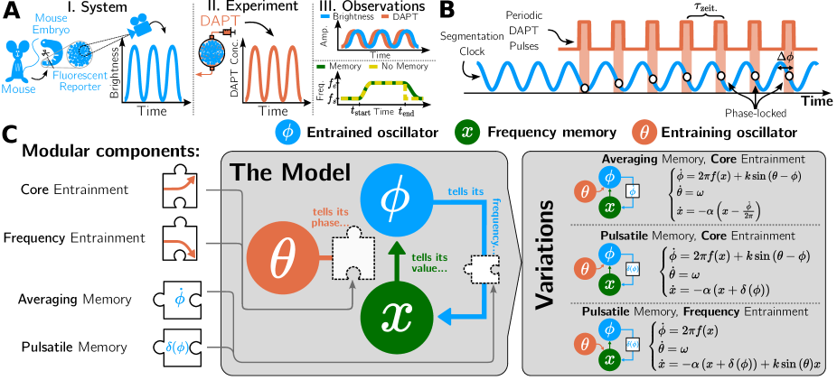
Figure 1: A) Sanchez et al Sanchez et al. (2022) studied notch oscillations in the mouse embryo tailbud. They managed to entrain these to external periodic pulses of DAPT. Experiments, where the system was "released" from the entraining signal, revealed that the embryonic oscillator adapts its internal frequency. B) Periodic perturbation of the segmentation clock via DAPT (period $\tau$) in presomitic tissue results in entrainment of the clock with measurable entrainment phase, $\Delta\phi$. C) The model we study has three interconnected dynamical variables. They are the entrained oscillator (blue), the entraining oscillator (orange), and the memory variable $x$ (green). The types of interconnections are modular and give rise to the variations of the model.

II Results

II.1 Modelling phase oscillators with frequency memory

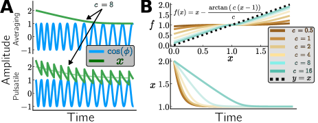
Figure 2: Behavior and conditions for models with a memory variable A) The two plots show examples of frequency convergence when starting away from the stable state for the Averaging memory system (top) and the Pulsatile memory system (bottom). $\alpha=1$. B) Examples of possible coupling functions, with $c_{1}=c_{2}=c$ for $f$ and their associated decay rates (for the Averaging-Core system). When $f\sim x$, $x$ decays linearly, while when $f\sim 1$, $x$ decays exponentially. $\alpha=1$.

We aim to formulate the problem of phase oscillators with memory in the simplest possible way. We consider a generic phase oscillator, called $\phi$, which in the absence of other variables would correspond to a classical "clock". However, we assume that the frequency of this oscillator called $f$, depends on another variable called $x$, which can be any biological parameter of the system (e.g. some metabolite concentration, a degradation rate, etc.). A natural choice might a priori be to assume that $f(x)\sim x$, i.e. that one variable $x$ in the system directly fixes the frequency so that the introduction of an extra step $f$ might seem unnecessary. However, we will see below that in the presence of feedback, one indeed needs an additional non-linearity for the system to be stable, justifying the introduction of such an intermediate.

Indeed, our key additional assumption is that $x(t)$ is some function of previous phases $\phi(u),u\leq t$, thus storing a memory of the past of the clock. Since the frequency $f$ is a function of $x$, changes of $x$ possibly lead to frequency changes. Such a model is in particular inspired by what is observed in the segmentation clock, where at least two oscillating pathways, Notch and Wnt, were suggested to influence their respective periods and can entrain one another Sonnen et al. (2018); Lauschke et al. (2013); François and Mochulska (2024), reminiscent of models of positional information based on the computing of phase difference Goodwin and Cohen (1969); Beaupeux and François (2016). Notice that $\phi$ and $x$ are of a different nature: $\phi$ is a phase variable, effectively capturing in an abstract way the state of the system Kuramoto (1984), while $x$ is an observable variable of the system such as the concentration of a protein.

We study two types of couplings between $\phi$ and $x$, conceptualized in Fig. 1 C.

II.1.1 Averaged memory

In the first instance, we consider a model with "averaged memory":

$$\begin{cases}\dot{\phi}=2\pi f(x)\\ \dot{x}=\alpha\left(\frac{\dot{\phi}}{2\pi}-x\right).\end{cases}$$ (1)

where $\alpha$ sets the timescale of convergence for $x$. $x$ acts as a smooth averaging of the past frequency in the limit of small $\alpha$. Since $x$, in turn, influences $\phi$, the function $f$ can not be arbitrary. In the absence of any other external signal, one gets for $x$

$$\dot{x}=\alpha(f(x)-x)$$ (2)

which should have at least one stable fixed point $x_{*}=f(x_{*})$, defining the natural intrinsic frequency $\omega_{i}=2\pi x_{*}$. In the following, we rescale time and $x$ so that $x_{*}=1$. Thus, we also have for the intrinsic frequency $f_{i}=1$ and the corresponding intrinsic period $\tau_{i}=1$. Stability further imposes that $f^{\prime}(x_{*})<1$. This means that $f$ has to be sublinear close to the fixed point: for $x>1$, the system slows down to decrease its frequency towards $1$ while for $x<1$ the system speeds up.

Figs. 2A,B show the dynamics of such oscillator following a perturbation in $x$ (all simulations presented are available in a Jupyter Notebook, https://github.com/cmdenis/2024-frequency-memory, see Appendix B for more details). As said above, a natural choice for $f$ would be $f(x)\sim x$, which would give $f^{\prime}(1)=1$ but thus is only marginally stable. To circumvent such marginal stability, we define

$$f(x)=x+\sigma(x)$$ (3)

where $\sigma(x)$ is a sigmoid function capturing the non-linearity of $f$ with respect to the internal memory. The conditions $f(1)=1,f^{\prime}(1)<1$ translate into $\sigma(1)=0,\sigma^{\prime}(1)<0$. Remarkably, we will show below that multiple aspects of entrainment depend simply on the non-linearity $\sigma(x)=f(x)-x$, further justifying the introduction of such a function.

We typically consider small $\sigma$ so that $f(x)$ is a small perturbation of the memory variable $x$ controlling the frequency. In the following, we consider functions of the form

$$\sigma(x)=-\frac{\arctan c_{2}(x-1)}{c_{1}}$$ (4)

where $c_{1}$ and $c_{2}$ are positive constants, as illustrated in Fig. 2 B, which ensures that $\sigma^{\prime}(1)<0$. Big $c_{1}$ ensures only weak non-linearity. Except otherwise mentioned, in simulations we set $c_{1}=c_{2}=8$. Notice also that, for such a choice of $\sigma$ and small and big $x$, $f$ is linear in $x$ up to an additive constant.

II.1.2 Pulsatile memory

The coupling above relies on an implicit averaging of phase dynamics by $x$, which might be difficult to implement biologically because the phase is an abstract variable associated with a limit cycle. We thus propose and study a more mechanistic model for such coupling. It has been recently observed that the coordination of gene expression can be done through pulsatile activations, which provide a natural, and possibly ubiquitous mechanism for frequency sensing by biochemical networks Cai et al. (2008). The segmentation clock itself seems to present features of pulsatile behaviors Eck et al. (2024), which is also consistent with the idea that it is poised close to a SNIC bifurcation Jutras-Dubé et al. (2020), known to naturally display pulsatile dynamics (type I oscillators Izhikevich (2007); François and Mochulska (2024)). Motivated by those observations and the model proposed in Cai et al. (2008), we introduce a "pulsatile coupling" model, where pulses in the $x$ variable are generated at a specific phase for $\phi$. Biologically, this could be done for instance, at the maximal value of some oscillatory variable, or if the oscillating system described by $\phi$ is itself pulsatile, this can be done at the pulse itself. We thus study the resulting ODEs:

$$\begin{cases}\dot{\phi}=&2\pi f(x)\\ \dot{x}=&\alpha\left(r\delta\left(\textbf{mod}(\phi,2\pi)\right)-x\right).\end{cases}$$ (5)

$\delta$ is the Dirac delta function centered around 0, and for convenience, we also define $r\alpha$ as the magnitude of the pulse. To get an intuition for this system, one can think of what happens in the limiting cases. If $\phi$ completes many cycles in a given amount of time, then the pulses begin to "stack up" raising the average value of $x$ since it doesn’t get the chance to decrease significantly. Conversely, if very few cycles are completed by $\phi$ in that same amount of time, then $x$ will have the time to decay closer to 0, which will make the average value of $x$ low. All in all, such a mechanism allows $\phi$ to modulate the level of $x$.

Notice that in the pulsatile model, $x$ is oscillating as well, at the same frequency as $\phi$, a situation again reminiscent of somitogenesis with the coupling of multiple biological oscillators Sonnen et al. (2018); Goldbeter and Pourquié (2008). Similar to the averaging coupling case, $r$ can not be arbitrary for stability. By integrating Eq. 5 over one period with periodic x, one gets

$$0=-\langle x\rangle+\frac{r}{\tau_{i}}$$ (6)

where we define $\langle x\rangle=\frac{1}{\tau_{i}}{\int_{0}^{\tau_{i}}}x(t)dt$ the average value of $x$ over one period. If we take for the stable period $\tau_{i}\sim 1$ and similar to the averaged memory case $\langle x\rangle=1$, we then get $r=1$, the choice we make throughout this work . Other choices are possible for the same $f(x)$ but would then simply change the stable frequency of the oscillator, which can then be put back to $1$ by rescaling time (Appendix C, Fig. S1 for different choices of parameters). Given some initial conditions away from the stable state, the system gradually adjusts its frequency to converge back to the stable long-term frequency, at a rate proportional to $\alpha$, as shown in Fig. 2A bottom.

II.2 Entrainment of the core oscillator $\phi$

Interesting properties occur when those models are perturbed. For a standard limit cycle oscillator, classical entrainment theory reduces to a one-dimensional phase equation reproduced in Appendix A, Eq. 23. However, with two oscillating variables ($\phi,x$), the system becomes "unclocklike" and new entrainment modalities appear.

We first focus on entrainment on the intrinsic phase $\phi$, which we refer to as the "core" oscillator. We introduce an external oscillator $\theta$, with frequency $\omega$, and introduce a coupling function $H$ and a coupling constant $k$ such that the modified equations are :

$$\begin{cases}\dot{\phi}=2\pi f(x)+\underbrace{k\ H(\theta-\phi)}_{\text{Core Entrainment}}\\ \dot{\theta}=\omega\\ \end{cases}$$ (7)

with $x$ dynamics prescribed by either Eq.1 or Eq. 5 depending on the internal coupling model considered. For convenience, we also define the entrainment period $\tau=\frac{2\pi}{\omega}$.

Fig. 3A illustrates how both Averaged and Pulsatile memory models are entrained by the external oscillator using one of the functions defined in Fig 2B, and a standard Kuramoto coupling $H=\sin$. Of note, the value of $x$ is changing due to entrainment. Since $x$ is both a measure and a control of the internal frequency of the phase oscillator (via the weakly nonlinear function $f(x)=x+\sigma(x)$ with small $\sigma$), it means that the system is adapting its intrinsic frequency in response to the external oscillator.

Fig. 3B, middle, illustrates the advantage and versatility of systems with frequency adaptation: when ramping up the frequency $\omega$ of the external oscillator $\theta$, the system can dynamically adjust its frequency to follow the external oscillator over a broad range of frequencies. We contrast this behavior with the standard case, where the internal frequency is maintained to $1$ where the system is only entrained for the range of $f$ defined by $2\pi|1-f|<1$ (from Appendix, Eq. 24 taking $\omega_{i}=2\pi$ and $H=\sin$), Fig. 3B, bottom.

II.3 Arnold Tongues and hysteresis for Core entrainment

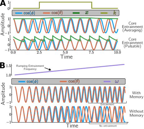
Figure 3: A) Comparison of different entrainment systems. Each subplot is divided into different regimes. Initially, the system is unentrained. Once the coupling is activated, the two oscillators enter a transient state before eventually becoming synchronized. When the coupling is removed, $\phi$ returns to its stable frequency/period. Middle subplot: Entraining $\phi$ with $\theta$ using the Averaging-Core system. Bottom subplot: Entraining $\phi$ with $\theta$ using the Pulsatile-Core system. $\omega/(2\pi)=1.1$, $\alpha=1$. B) Comparison between a system with memory and a system with no memory, if entrained by an external oscillator whose frequency is ramped up, with $k=1.5$, $\alpha=5$.

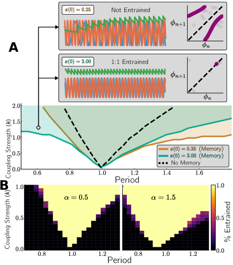
Figure 4: A) Arnold tongues for the Pulsatile-Core system with memory for different initial conditions and system with no memory. The system with memory has wider tongues. We show sample runs and the effect initial conditions have on entrainment. The Arnold tongue was computed numerically by checking the convergence of phase $\phi$ using stroboscopic maps over 2000 cycles, as illustrated on the top. $\alpha=0.5$. B) Probabilistic Arnold Tongue for the Pulsatile-Core system with $\alpha=0.5$ and $\alpha=1.5$. Varying the $\alpha$ parameter affects the width of the tongue. $x(0)=1.1$.

Fig. 4 displays the entrainment range of oscillators as a function of the rescaled period $2\pi/\omega$ and of the coupling strength $k$ for $H=\sin$, generally called "Arnold tongues" Glass (2001), displayed here for the pulsatile system, (see Appendix D, Fig. S2 for equivalent tongues with averaged memory), for different initial conditions of the system. Fig. 4 A illustrates the range of possible entrainment for various values of initial $x$ (a set of parameters is labeled as entrained if numerically a $\phi(t=0)$ is found that makes the trajectory entrained), while Fig. 4 B shows what happens for a fixed initial value of $x=1$ as we vary the initial condition for the phase $\phi(t=0)$, and $\alpha$. A comparison with the same system with a fixed $f=1$ (no memory) is shown in Fig. 4A. Focusing first on Fig. 4 A, the tongue for the system with memory widens for higher coupling strength compared to the equivalent one without memory, meaning that the system is much easier to entrain as already illustrated in Fig. 3. This is reminiscent of the large tongues obtained for the segmentation clock in Sanchez et al. (2022). However, we further observe that the initial conditions for $x$ strongly matter to have entrainment within a given tongue, a new "unclocklike" property of such systems. Simulations that started with lower initial $x$ can usually get entrained to lower periods, and simulations that started with higher initial $x$ can get entrained to higher periods, Fig. 4A. This creates the first type of hysteresis where the entrained/not entrained state depends on the history of the system via $x$, as further illustrated in Fig. 5. We show two different protocols: in the top of Fig. 5 A, the angular velocity of the external oscillations ($\omega$) is started at the natural intrinsic value corresponding to $f=x=1$, and then slowly increases by $50\%$ while keeping the system entrained. However, if this angular velocity is suddenly changed from the same initial condition, the system does not entrain, Fig. 5 A bottom. In Appendix E, Fig. S3 shows a similar behavior for the Averaging-Core system when ramping the entrainment frequency at different rates. Conversely, one can keep $x$ constant and change the initial phase of $\phi$, to observe probabilistic Arnold tongues, Fig. 4B. In particular, close to the boundaries of the entrainment range, some initial phase conditions do not allow for entrainment because $x$ is pushed at too low or too high values, and the effect is stronger for bigger $\alpha$ because $x$ varies much more in such cases (see below). Again, such initial condition dependencies are not possible in classical phase response theory, because entrainment is associated with a fixed point equation on the phase, which either has a solution or not. Another form of hysteresis is observed for the pulsatile system, with a new kind of bistability compared to classical entrainment theory, illustrated in Fig. 5B. Classically, a $1:1$ tongue is observed if the frequency of the external oscillator $\theta$ is close to the intrinsic frequency of the oscillator $\phi$. However, if the $x$ variable is perturbed, new entrainment regimes appear as the intrinsic frequency of the oscillator changes because of the feedback. For instance, if $x$ is initialized at a low value, this poises the oscillator toward low frequency, and one can observe a $1:2$ tongue, even if the external oscillator oscillates at the stable intrinsic frequency $f=1$. Here, importantly, the system displays bistability in its intrinsic frequency $f(x)$ due to the feedback between $\phi$ and $x$, which is impossible to observe in standard models where $f$ is constant. Bistability is one of the hallmarks of internal feedback in stable biological systems Cherry and Adler (2000): thus, feedback here creates a new type of bistability for an oscillating system.

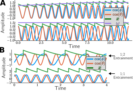
Figure 5: A) Experimental scheme to test for hysteresis. Parameters are $k=1.8$, $\alpha=0.5$. (Top) For the Pulsatile-Core system, the entrainment frequency ($\omega/(2\pi)$) is started at 1 and slowly ramped up to 1.5: entrainment persists. (Bottom) The system’s entrainment frequency ($\omega/(2\pi)$) is started immediately at 1.5: no entrainment. B) Example of bistability in the pulsatile frequency coupling system. The same parameters with different initial conditions give rise to different cyclic outcomes. It is possible to entrain the system to 1:1 (bottom) and 1:2 (top) regimes, depending on the initial conditions for the memory variable $x$. $\omega/(2\pi)=2.2$, $k=1.5$.

II.4 Phase of entrainment

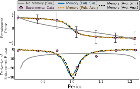
Figure 6: (Top) Entrainment phase for models with memory (core entrainment) and without memory, fitted to the experimental data. The models with memory all present the same overlapping shape. The black dotted curve is the analytically computed phase difference Eq. 10 (indistinguishable from the equivalent simulated results), which perfectly overlaps with the simulated pulsatile-core system (blue) and Eq. 14 (diamond yellow). This contrasts with the $\arcsin$ shape of the system without memory, Eq. 25. For comparison with experiments, we shifted the (arbitrary) phase definition of experimental data for $\theta$ so that $\Delta\phi=0$ for a rescaled period of $1$. Parameters for memory system: $c_{1}=7.6$, $c_{2}=53.6$, $k=1.35$, $\alpha=0.03$, $\tau_{\text{scale}}=147.5$. Parameters for the system without memory: $k=1.3$, $\tau_{\text{scale}}=144$. (Bottom) Derivative of the entrainment phase for the system with memory, without memory, and the experimental data, where slight differences between simulations and models are more visible.

An important observable associated with entrainment is the stationary phase difference $\Delta\phi=\theta-\phi$ between entrained and entraining oscillators, Fig. 6. Importantly, such phase differences are much easier to measure experimentally with low uncertainty compared to other variables or Arnold Tongue boundaries Sanchez et al. (2022), and as such constitute one of the best ways to discriminate between different models.

II.4.1 Averaged memory

Studying first the averaged memory model, and assuming that at entrainment $x=x_{c}$ is approximately constant (which is approximately the case if $\alpha$ is small), and that $\Delta\phi=\theta-\phi$ is constant meaning that $\dot{\phi}=\omega$, we get :

$$\omega=2\pi f(x_{c})+kH\left(\Delta\phi\right)$$ (8)

It also follows from Eq. 1 at stationarity that

$$x_{c}=\frac{\dot{\phi}}{2\pi}=\frac{\omega}{2\pi}=\frac{1}{\tau}$$ (9)

so that $x$ is indeed a direct measure of the external frequency, as expected by construction.

We can then invert Eq. 8 to get :

$$\Delta\phi=H^{-1}\left(\frac{-2\pi\sigma(\frac{\omega}{2\pi})}{k}\right)$$ (10)

where $\sigma(x)=f(x)-x$ measures the deviation between $f$ and a pure linear behavior. Notice that, remarkably, the entrainment phase thus provides a direct measurement of the non-linearity $\sigma(x)$ (assuming $H$ is known).

In experiments on the segmentation clock Sanchez et al. (2022), data fitting suggests that the change of internal frequency with detuning $df/d\omega$ is approximately $1$ for high and low periods. This means that $\sigma$ converges to constant values for high and low $x$, thus justifying the sigmoid form defined in Eq. 4. From Eq. 10, we expect convergence of the entrained phase towards constant values at low and high periods. Those values are free parameters of the model but can be fitted so that simulations are in full agreement with the experimental data reproduced in Fig. 6, using $H=\sin$. This result is to be contrasted with the classical entrainment that predicts infinite derivatives at the boundaries of the entrainment ranges in such regimes (Fig. 6, gray line, and Appendix A). One could be concerned that such plateauing would come from the perfectly linear asymptotic behavior of $f$, in Appendix F, Fig. S4 we illustrate what happens for different asymptotic slopes, and we still observe sigmoid shapes consistent with experiments for a broad range of periods.

II.4.2 Pulsatile memory

For the pulsatile system, similar analytical results can be obtained, see details in Appendix G. Assuming the oscillator is entrained, we can integrate equations over one cycle (from $t=0$ to $t=\tau$, the entrained period). Recalling that $f(x)=x+\sigma(x)$, we get from the $\phi$ equation

$$\omega=2\pi\langle x\rangle+2\pi\langle\sigma(x)\rangle+k\langle H(\Delta\phi)\rangle.$$ (11)

Using the periodicity of $x$ and taking the origin of time $t=0$ right after the pulse of magnitude $r\alpha$, we can integrate the $x$ equation over one cycle to get

$$x(t)=r\alpha\frac{e^{-\alpha t}}{1-e^{-\alpha\tau}}.$$ (12)

In particular, we see that $\int_{0}^{\tau}x(t)dt=\frac{r\alpha}{\alpha}=r=1$, which gives the very intuitive results that $x$ varies around its steady state value in absence of entrainment $x\sim 1$. We also see that $\langle x\rangle=\frac{1}{\tau}=\omega/(2\pi)$, showing that, due to entrainment, $x$ adjusts to match the entrainment frequency on average, similar to the averaged memory case (Eq. 9) even though $x$ is not constant in that case.

Injecting into Eq. 11, the $\omega$ terms cancel out and we get

$$0=\langle\sigma(x)\rangle+\frac{k}{2\pi}\langle H(\Delta\phi)\rangle.$$ (13)

Remarkably again, this equation relates intuitively and compactly the entrained phase difference between the two oscillators $\Delta\phi$ to the non-linearity of the internal frequency $f$, which is entirely captured by $\sigma(x)=f(x)-x$. Notice that Eq. 10 for averaged memory is a mean-field equivalent of Eq.13.

Further assuming now that $\Delta\phi$ (but not necessarily $\sigma$) is approximately constant over one cycle (see Appendix G), we can get a similar form as Eq. 10

$$\Delta\phi=H^{-1}\left(\frac{\left(\omega-\chi(\omega)\right)}{k}\right)$$ (14)

with $\chi(\omega)$ given by Eq. 32. In Appendix G we show that, for our choices of $f$, $d\chi(\omega)/d\omega\sim 1$ (Eq. 39) for high and low detuning, ensuring that in the pulsatile coupling case, $\Delta\phi$ plateaus in the same way as the averaging coupling case for high and low detuning.

In fact, assuming that $\alpha$ is small, we can see from Eq. 12 that $x$ is almost constant. At order $0$ in $\alpha$, we get back that $x\sim\frac{1}{\tau}$, and from Eq.13

$$H(\Delta\phi)=-\frac{2\pi}{k}\sigma(x)$$ (15)

which consistently turns out to be identical to the averaging coupling model result in Eq. 10. Thus in the limit of small $\alpha$, there is no difference between the pulsatile and averaged memory models for $\Delta\phi$ at steady state, suggesting that the computation of such phase difference is a good way to show the existence of an internal frequency memory irrespective of the model details.

Fig. 6 further shows the numerical and analytical phase curves for the two types of coupling and are further compared to a standard system without memory, and the experimental data presented in Sanchez et alSanchez et al. (2022).

II.5 Entrainment through the memory variable

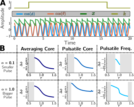
Figure 7: A) Example of entrainment for the pulsatile frequency system. The system is initially unentrained until the coupling is activated, after which it becomes entrained. The coupling is stopped afterward. The timescale of the entrainment is slower for the frequency entrainment than for the core entrainment. Notice the deformation of the $x$ curve by the sinusoidal coupling. $k=1.0$, $\alpha=1.0$, $\omega/(2\pi)=1.1$. B) Comparison of entrainment phases for the different models under consideration, with their entrainment ranges. The gray regions correspond to no entrainment. Simulations were all initialized with $x(0)=1$. Other examples of such curves for different couplings are qualitatively identical or similar and shown in Appendix H $k=1.5$.

It is natural to investigate entrainment performed on $x$, the memory variable (instead of $\phi$). If $f$ is weakly non-linear, we intuitively expect $x$ to be more directly related to the frequency, so it is not clear that $x$ has enough phase dependency to allow for entrainment, which should consequently be harder. Indeed, we could not entrain the averaged memory model, probably because of the explicit averaging performed by $x$ which erases any phase information.

In the pulsatile system, $x$ is oscillating so contains more phase information. We study

$$\begin{cases}\dot{\phi}=&2\pi f(x)\\ \dot{x}=&\alpha\left(\underbrace{r\delta\left(\textbf{mod}(\phi,2\pi)\right)}_{\text{Pulses}}-x\right)+\underbrace{k\sin\left(\theta\right)x}_{\text{Freq. Entrainment}},\end{cases}$$ (16)

which allows for an explicit analytic expression of $x$ if there is entrainment (see Appendix I and Eq. 20).

Entrainment on this system is illustrated in Fig. 7A and Fig. 7B further compares various entrainment modalities. For small $\alpha=0.1$ we observe a much smaller entrainment range for frequency entrainment compared to the core oscillator, and an associated smaller range of possible $\Delta\phi$. This is consistent with the fact that $x$ still erases much of the phase information: it is indeed difficult to entrain, and the system must be adjusted to a specific phase to do so.

To understand what happens, it is again useful to integrate Eq. 16 over one cycle right after the pulse in $x$ to get

$$\int_{0}^{\tau}\dot{\phi}dt = 2\pi\int_{0}^{\tau}f(x)dt$$ (17)

$$\int_{0}^{\tau}\dot{x}dt = -\alpha\int_{0}^{\tau}x(t)dt+k\int_{0}^{\tau}\sin(\omega t+\Delta\phi)xdt$$ (18)

where we introduced the phase shift $\Delta\phi$ between the entraining signal and the system (so that $\phi=0$ corresponds to the time of the pulse). This way, we can rewrite $\theta(t)=\omega t+\Delta\phi$.

Focusing on Eq. 18, the left-hand side of this expression is $-r\alpha$ because of the periodicity of the system and the pulse of magnitude $r\alpha$ in $x$ at $t=0$. For the first term on the right-hand side, we use Eq. 3 to notice that $\int_{0}^{\tau}xdt=\int_{0}^{\tau}f(x)dt-\int_{0}^{\tau}\sigma(x)dt$, and from Eq. 17 $\int_{0}^{\tau}f(x)dt=\frac{1}{2\pi}\int_{0}^{\tau}\dot{\phi}=1$. Given that $r=1$, the $r\alpha$ and $\alpha$ terms cancel out and we get

$$\langle\sin(\omega t+\Delta\phi)x(t)\rangle=\frac{\alpha}{k}\langle\sigma(x(t))\rangle$$ (19)

which is reminiscent of Eq. 13. Notice that in the limit of small $\alpha$ the right-hand side of Eq. 19 is expected to be rather small, which is consistent with the fact that we expect entrainment to be difficult in this limit.

To go further one can integrate $x(t)$ to get (assuming $t=0$ corresponds to the pulse):

$$x(t)=\frac{\alpha e^{-\alpha t}}{1-e^{-\alpha\tau}}\exp{\frac{k}{\omega}[\cos(\Delta\phi)-\cos(\Delta\phi+\omega t)]}.$$ (20)

Notice that $x$ depends on $\Delta\phi$ because the pulse happens at $t=0$. Substituting the value of $x$ into Eq. 19 provides an analytic expression allowing to define $\Delta\phi$ implicitly (see Appendix I for the full expression). Like before, the stationary phase difference $\Delta\phi$ thus is a pure function of $\sigma$. The expression is highly non-linear and can not be inverted analytically, however, it can be solved numerically and compared to the steady-state value of the phase shift from explicit entrainment simulations, with perfect agreement, see Appendix I, Fig. S6.

To get a better sense of what happens, further approximations are needed. For low $\alpha$ Taylor expansion of the left-hand side of Eq. 19 gives

$$\langle\sin(\omega t+\Delta\phi)x(t)\rangle=\frac{\alpha}{k}\left(I_{0}\left(\frac{k}{\omega}\right)e^{\frac{k\cos(\Delta\phi)}{\omega}}-1\right)$$ (21)

where $I_{0}(x)$ is the modified Bessel function of the first kind of order zero. This expression is proportional to $\frac{\alpha}{k}$ which thus simplifies with the right-hand side of Eq. 19. One can use this Taylor expression to invert $\Delta\phi$, again with very good agreement Appendix Fig. S6.

We notice that $\Delta\phi$ depends only weakly on the detuning, indicative that the systems closely follow the entrainment signal in such a frequency coupling regime. This means that we can get a zero-order approximation of $\Delta\phi$ by taking its value for detuning $0$ (i.e. $\omega=2\pi$) so that $\langle\sigma\rangle=0$, which gives

$$\Delta\phi\sim\arccos\left(-\frac{2\pi}{k}\ln\left(\text{I}_{0}\left(\frac{k}{2\pi}\right)\right)\right)-\pi$$ (22)

which is close to $-\pi/2$ for $k\sim 1$. For non-zero detuning, $\sigma$ remains small because $x$ oscillates close to $1$, and $I_{0}\left(k/\omega\right)$ stays of order $1$ which is the reason why $\Delta\phi$ does not change much with the detuning, and consistent with the idea that the entrained system is poised to a precise phase difference in this regime, Appendix I Fig. S6.

II.6 Large $\alpha$ regime

So far we have implicitly assumed that $\alpha$ is small, which is necessary to have a weakly oscillating $x$, leading to a well-defined $f$ throughout the cycle. We are now relaxing this assumption to explore the limit of large $\alpha$.

In the averaged memory regime, taking in Eqs. 1 and 7 the quasi-static approximation $x\sim\frac{\dot{\phi}}{2\pi}$ gives $x\sim f(x)+\frac{k}{2\pi}H(\Delta\phi)$, which is the same equation as for the small $\alpha$ regime. So we do not expect any difference for the phase difference $\Delta\phi$ at entrainment for small and large $\alpha$, as indeed seen numerically in the first column of Fig. 7 B.

However, for the pulsatile memory, the high $\alpha$ regime is different from the low $\alpha$ regime. The reason is that the magnitude of the pulse is proportional to $\alpha$. Because of this, $x$ becomes initially very big, but since the existence of the limit cycle requires that the average value of $x$ is $1$ (in the absence of entrainment), $x$ also needs to decay below $1$ significantly. Consequently, $f(x)$ varies much over one cycle. Thus, the system oscillates in a qualitatively different way: $\phi$ progresses rapidly right after the pulse but much more slowly when $x$ is decaying below $1$, as seen in Fig. 8 A (compare $\alpha=0.5$ where $\cos\phi$ is very sinusoidal to $\alpha=5.0$ where it is more "sawtooth"-like).

In particular, the stable unentrained period depends on $\alpha$ in this regime, and can further be analytically computed. We assume that $x$ varies as $x(t)\sim\alpha e^{-\alpha t}$ for large $\alpha$. Assuming quick transitions between the plateaus of the sigmoid $\sigma$ we obtain the relation $\tau^{*}=2\frac{\log\alpha}{\alpha}$ (see Appendix J for derivation). Fig 8 B shows the comparison between this approximation and the measured period in simulations, with an excellent agreement for high enough $\alpha$.

Because of the non-uniform progression of $\phi$, entrainment properties are largely modified, and analytical results are more difficult to obtain. For entrainment on the core oscillator $\phi$, for long entrainment periods, the entrainment phase does not depend much on detuning and is approximately $0$, Fig. 7B, bottom middle. This is not surprising since for high $\alpha$, $\phi$ spends much time right before the pulse time $\phi=0$ as can be seen in Fig 8 A, and thus $\theta$ aligns with this point. For frequency coupling, there is now much more information on the global phase of the oscillator in the variable memory $x$ in this case, and remarkably, one recovers a plateauing dependency similar to the core coupling at low $\alpha$, Fig. 7B, bottom right. Notice however that, since $\dot{\phi}$ can no longer be considered uniform over a cycle for big $\alpha$, $\phi$ can no longer be directly taken as the ’true’ oscillator phase Kuramoto (1984). Such non-uniform phase increase is rather reminiscent of oscillators tuned close to an infinite period bifurcation François and Mochulska (2024) or the ERICA model for somitogenesis proposed in Sanchez et al. (2022), with strong influences on the shape of the Phase Response Curve.

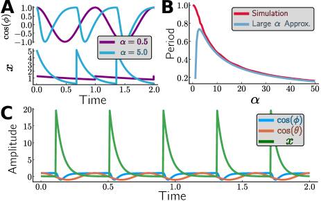
Figure 8: A) Unentrained time evolution of $\cos(\phi)$ and $x$ for the pulsatile systems, for different values of $\alpha$. Higher $\alpha$ leads to shorter stable unentrained periods (higher frequency) and asymmetric oscillations. B) Simulation and analytical approximation for the stable unentrained period for the Pulsatile system. This applies to both the Pulsatile-Core and the Pulsatile-Frequency system since this is for the unentrained system. C) Example of entrainment of a high $\alpha$ system for Pulsatile-Core system. The range of 1:1 entrainment gets shifted to shorter periods. $k=1$, $\alpha=20$, $\omega/(2\pi)=2.5$.

III Discussion

In this work, we propose and study simple models of "unclocklike" oscillators with an internal memory variable. We are motivated by unexpected properties of the embryonic segmentation clock in response to entrainment Sanchez et al. (2022), and by the more general idea that some biochemical memory variable $x$ is controlling the internal frequency $f(x)$ of the oscillator, while itself oscillating. We observe new entrainment properties that can not be captured with classical entrainment theory, because it precisely lacks such memory.

Formalizing the problem of frequency adaptation allows us to explore necessary conditions and suggests new effects. Simple fixed point analysis shows that the frequency $f(x)$ of the core oscillator $\phi$ has to be sublinear in the memory variable $x$, close to its natural frequency. It makes intuitive sense: for instance, if the frequency of the system were to be slightly increased externally by some transient perturbations, it then has to go down closer to its natural frequency, thus ensuring homeostasis. The effect of such frequency adaptation is mostly visible in entrainment experiments. It first allows for a considerably bigger entrainment range with broad Arnold tongues, Fig. 4. Furthermore, in all models considered, the entrainment phase is always a function of the non-linearity of the frequency, captured by the function $\sigma(x)=f(x)-x$. This observation is of practical importance. Concretely, an experimentalist could vary the frequency of entrainment $\omega$, measuring the entrainment phase difference $\Delta\phi$ to infer properties of both the coupling functions $H$ and non-linearity in the frequency $\sigma$, which quantifies the feedback between the memory variable and the frequency of the oscillator. Case in point, in the vertebrate segmentation clock Sanchez et al. (2022), the shape of $H$ was first inferred, then the plateauing of $\Delta\phi$ suggested both the existence of such feedback and its functional form, i.e. $f(x)=x\pm c_{1}$ for high detuning and low. Systematic explorations of different biological oscillators might reveal different types of $\sigma$ corresponding to different internal controls.

We also demonstrate two new hysteretic effects associated with such models. Exploring the full entrainment range is only possible with a smooth change of frequencies, allowing to adiabatically change the memory variable $x$. Conversely, if one suddenly changes the frequency of entrainment close to the boundary of the entrainment range, $x$ can not rapidly adapt so that entrainment is impossible. This is the first new hysteresis type: entrainment with high detuning depends on the past history of $x$, Fig. 5 A. Another hysteretic effect is bistability in the intrinsic frequency of the oscillator, depending on the value of $x$ Fig. 5 B, where in particular the system can adopt a frequency twice as slow as the imposed intrinsic frequency. In the segmentation clock entrainment context, one could imagine combining the two hysteretic effects within one single experiment: one could slowly decrease the entrainment frequency by a factor of $2$, ensuring the intrinsic period is double, before suddenly reverting to the intrinsic frequency of the oscillator, thus ensuring 1:2 entrainment. Entrainment appears more difficult through $x$ than through $\phi$, possibly because the phase effects on $x$ are averaged by $f$, leading to a situation closer to overdrive suppression where the behavior is best explained by a simple change of one internal parameter Zheng and Wang (2015). In the segmentation clock context, entrainment experiments have been done via perturbations of Wnt, Notch Sonnen et al. (2018) and metabolism, which acts via Wnt Miyazawa et al. (2024). The comparison of entrainment ranges and entrainment phases for each of those situations might help to uncover qualitative differences in entrainment properties, possibly identifying pathways responsible for different organization levels in the biological "unclock" considered (i.e. core clock $\phi$ vs memory variable $x$). It is already known that Wnt and Notch relative phases have a functional role in differentiation Sonnen et al. (2018). Thus, a single phase cannot fully describe the segmentation clock, which is "unclocklike". It has further been suggested that a second oscillator (possibly Wnt) changes the frequency of the Notch oscillator Lauschke et al. (2013). Interestingly, Wnt oscillations are experimentally much more synchronized within the embryo than Notch Sonnen et al. (2018), a possible indication that Wnt could indeed implement and encode some averaging of Notch oscillators, thus possibly playing a role similar to the memory variable $x$.

Progress in quantitative biology and real-time imaging has opened the door for systematic exploration, modeling, and understanding of biological dynamics. In some cases, one can directly relate biology to well-known, classical mathematical descriptions (e.g. landscapes Rand et al. (2021)), and theoretical modeling involves mapping mathematical control parameters to biological handles. However dynamical systems in biology are often more versatile and adaptive than classical physics ones. A more complete understanding requires specific hypotheses tied to uniquely biological properties, such as homeostasis, adaptation, or more generally computation Koseska and Bastiaens (2017). Memory variables like those proposed here explain how the time scale of biological oscillators can adjust to external constraints, possibly contributing to the labile tempo of embryonic developmentEbisuya and Briscoe (2024); Manser and Perez-Carrasco (2023). Well-defined perturbations, such as entrainment, reveal properties of the internal biological feedbacks like memory variables. This opens the door for the building and the exploration of new classes of models like we do here, and further interactions between theory and experiments.

Appendix A Brief summary of classical entrainment theory

In this section, we briefly summarize aspects of classical entrainment theory of limit cycles to derive equations used for comparison in the main text. The phase of a clock is a zero mode on a limit cycle Pikovsky et al. (2001), and it can be shown that at the lowest order, assuming weak coupling, the dynamics of the entrained oscillator (phase $\phi$, intrinsic frequency $\omega_{i}$) are influenced by the entraining periodic signal (phase $\theta$, frequency $\omega$ ) in the following way :

$$\frac{d\phi}{dt}=\omega_{i}+H(\theta-\phi)$$ (23)

where $H$ is a function of phase (difference) that depends only on the shape of the flow of the entrained oscillator close to the limit cycle. For the segmentation clock, although DAPT pulses are only weakly influencing the oscillation , $H$ is strongly shifted depending on external oscillator frequency, which is not expected from classical theory since $H$ does not depend on $\omega$ in Eq. 23. Practically, this leads to "Arnold tongues" for entrainment much larger than usual Sanchez et al. (2022). Another inconsistency with the classical entrainment theory is the unusual behavior of the entrainment phase as a function of detuning Granada et al. (2013). Assuming that the external oscillator $\theta$ has frequency $\omega$, from Eq. 23 entrainment occurs if

$$\omega_{i}-\omega+H(\theta-\phi)=0$$ (24)

This means the range of entrainment is defined by maxima and minima of $H$, where the derivative $H^{\prime}$ is $0$. Furthermore, the relative entrainment phase of the oscillator $\phi_{e}$ with respect to the entrainment signal $\theta$ is thus of the form

$$\phi_{e}-\theta=H^{-1}\left(\frac{\omega_{i}-\omega}{c}\right)$$ (25)

then, $d\phi_{e}/d\omega$ is proportional to $1/H^{\prime}$ at the range of entrainment, so should become infinite (as illustrated in Fig. 6). Surprisingly, the entrainment phase for the segmentation oscillator plateaus for very small and very large detuning, thus completely inconsistent with the classical entrainment theory.

Appendix B Numerical Integration

All the simulations presented in this paper were done in the Julia programming language Bezanson et al. (2017), using the DifferentialEquations.jl package Rackauckas and Nie (2017).

The notebook to generate the data for all the figures in this paper (except conceptual Figs. 1 and S7) is available at the following repository: https://github.com/cmdenis/2024-frequency-memory

We used the built-in Vern9 and ROCK2 solver from DifferentialEquations.jl.

Appendix C Varying $r$

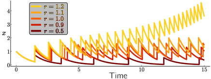
Figure S1: Effect of different ratios $r$, taking $\alpha=1$. Note that the system blows up (and speeds up) if $r$ is too big.

Varying the size of the pulse, through the $r$ parameter in the pulsatile system can give stable unentrained pulsation. However, it was seen numerically that high values of $r$ can start diverging numerically. For this reason as well as mathematical convenience we focus our attention on systems with $r=1$. Unentrained scenarios for $r\neq 1$ are presented in Fig. S1.

Appendix D Arnold Tongues for the Averaging-Core System

Just like the Pulsatile-Core system, we can obtain Arnold Tongues for the Averaging-Core system. We see the same behavior as in the pulsatile system when using different initial conditions for the $x$ variable in Fig. S2.

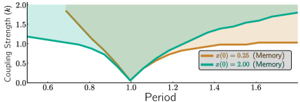
Figure S2: 1:1 Arnold tongue for the Averaging-Core system. Different initial conditions for the $x$ variable yield tongues stretching to shorter or longer periods. $\alpha=0.1$

Appendix E Core Coupling Hysteresis

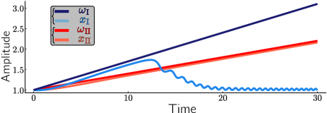
Figure S3: Example runs for the Averaging-Core system being entrained and unentrained after ramping the entraining frequencies. For an entrainment strength of $k=1.50$. Only the entraining frequencies ($\omega_{\text{I}}$ and $\omega_{\text{II}}$) and the internal frequency ($x_{\text{I}}$ and $x_{\text{II}}$) are shown. $k=1.5$, $\alpha=1$.

Hysteresis is noticed in the core coupling system. When varying the frequency of the entraining oscillator slow enough, we can entrain in a very wide range of frequencies. In fact, if the frequency is varied slowly enough and the amplitude of coupling is strong enough, no bound on the maximum frequency of entrainment was observed. Fig. S3 shows some quantitative results regarding the ramping of the frequency of the system.

Appendix F Variation of asymptotic behavior of the coupling function

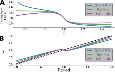
Figure S4: A) Coupling functions with different asymptotic behavior. For high or low $x$, curves go like $0.5x$, $1x$ and $2x$. $k=1.5$. B) Analytical curves using equation 10 for the entrainment phase curves resulting from the frequency curves $f$ presented in panel A, using core coupling with $H=\sin$.

We assumed that $f\sim x$ for $x$ away from 1, consistent with experiments. Such a precise constraint might however not always be realistic. However, we can relax this assumption to show that the system still possesses a characteristic flattening of its entrainment phase curve, as illustrated with numerical simulations in Fig. S4. If $f\sim ax$, then for $a>1$, there will be other points where $f(x)=x$ for $x\neq 1$, this means that there will be an infinite derivative at the end of the phase curve, but if $a$ is close to one, it will still be preceded by a flattening. If $a<1$, then the phase curve will not only flatten but also change the sign of its derivative past a maximum or minimum.

Appendix G Pulsatile Coupling Entrainment Phase

We consider the pulsatile regime

$$\begin{cases}\dot{\phi}=2\pi f(x)+kH\left(\theta-\phi\right)\\ \dot{x}=-\alpha x+r\alpha\delta\left(\textbf{mod}(\phi,\ 2\pi)\right).\end{cases}$$ (26)

Integrating the $\phi$ variable over one cycle

$$\frac{1}{\tau}\int_{0}^{\tau}\dot{\phi}\ dt=\frac{1}{\tau}\int_{0}^{\tau}\left(2\pi f(x)+kH(\theta-\phi)\right)\ dt.$$ (27)

We know that, $\frac{1}{\tau}\int_{0}^{\tau}\dot{\phi}\ dt=\frac{2\pi}{\tau}=\omega$. Hence we get

$$\omega=2\pi\langle f(x)\rangle+k\langle H(\Delta\phi)\rangle.$$ (28)

where averages are computed over one cycle.

Because the influence of $\phi$ over $x$ only occurs once every cycle, and assuming the system to be entrained, we can write explicitly the equation for $x$:

$$x(t)=e^{-\alpha t}(r\alpha+x_{0})$$ (29)

where $t$ is time, $r\alpha$ is the magnitude of the pulses, $\alpha$ is the decay rate and $x_{0}$ is the initial value of $x$ right after the pulse is applied corresponding to the beginning of the cycle $t=0$. Since we know the system is periodic, $x(\tau)=x_{0}$, and thus we have the equation :

$$x_{0}=\frac{r\alpha}{e^{\alpha\tau}-1}.$$ (30)

and

$$x(t)=r\alpha\frac{e^{-\alpha t}}{1-e^{-\alpha\tau}}.$$ (31)

We then define $\chi$ as

$$\chi=\omega\int_{0}^{\tau}f\left(r\alpha\frac{e^{-\alpha t}}{1-e^{-\alpha\tau}}\right)\ dt.$$ (32)

which can not be computed analytically without further assumptions. Assuming now that the phase difference $\Delta\phi$ between the two oscillators is roughly constant for the duration of the cycle (an assumption that we relax below), using the expression for $\phi$ in Eq. 5, we get

$$\Delta\phi=H^{-1}\left(\frac{\omega-\chi}{k}\right).$$ (33)

We can also use this expression to estimate the stable entrained frequency, $\omega^{*}$ by looking at the case where $\Delta\phi=0$ (assuming $H(0)=0$ corresponds to the stable coupling. This yields the relation

$$\omega^{*}=\omega\int_{0}^{\tau}f\left(r\alpha\frac{e^{-\alpha t}}{1-e^{-\alpha\frac{2\pi}{\omega^{*}}}}\right)dt.$$ (34)

Notice that in the limit of small $\alpha$ $\frac{e^{-\alpha t}}{1-e^{-\alpha\tau}}\rightarrow\frac{r\alpha}{\alpha\tau^{*}}$, so that

$$\omega^{*}=\omega f(\frac{r}{\tau^{*}})$$ (35)

For $r=1$ and $f(1)=1$, the intrinsic period $\tau^{*}=1$ is solution as desired.

One can also study what happens for high and low detuning. Assuming $f(x)=x+\sigma(x)$ where $\sigma$ is a sigmoidal function, and assuming saturation far from the intrinsic entrainment frequency, we can make the approximation

$$f(x)\approx x+C.$$ (36)

Hence, looking back at the expression for $\chi$ in the equation 32 and using the approximation in 36 we get

$$\chi=\omega\int_{0}^{\tau}\left(r\alpha\frac{e^{-\alpha t}}{1-e^{-\alpha\tau}}+C\right)dt$$ (37)

which yields

$$\chi=\frac{r\alpha}{\alpha}\omega+2\pi C.$$ (38)

so that

$$\frac{d\chi}{d\omega}\sim\frac{r\alpha}{\alpha}=r$$ (39)

as claimed in the main text.

Appendix H Varying the entrainment coupling function for the pulsatile-frequency system

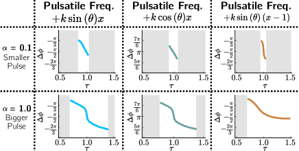
Figure S5: Phases of entrainment for different coupling terms in the Pulsatile-Frequency system with $k=1.5$.

We can create variations of the Pulsatile-Frequency model by modifying the coupling function used for entrainment between $\theta$ and $x$. In the main text, we presented a coupling function of the form $+k\sin\left(\theta\right)x$. Other variations such as $+k\cos\left(\theta\right)x$ and $+k\sin\left(\theta\right)(x-1)$ also yield entrainment. The phase of entrainment for these alternative systems is compared in Fig. S5, with qualitative behaviors similar to the case presented in the main text.

Appendix I Phase of entrainment for large $\alpha$ in pulsatile frequency system

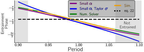
Figure S6: Phase of entrainment for the Pulsatile-Frequency system using different approximations. The yellow curve corresponds to the actual value of $\Delta\phi$ measured from full integration of the differential equations. The green curve corresponds to the numerical solving of the implicit Eq. 43 for $\Delta\phi$, which agrees perfectly with the simulations. The purple curve corresponds to the numerical solving of Eq. 43 after approximating the trajectory of $x(t)$ with a Taylor expansion for small $\alpha$. The blue curve corresponds to the numerical solving of Eq. 43 while linearizing $\sigma$ around 1 and using a Taylor expansion in $\alpha$ for $x(t)$. The dotted black curve corresponds to the constant value Eq. 22. For those simulations, we used $k=0.9$, $\alpha=0.1$, $c_{1}=8$, $c_{2}=4$.

We have shown analytical results for the phase of entrainment as a function of the period of the entraining oscillator. The phase of entrainment for the pulsatile-frequency system can be obtained in the limit of small $\alpha$. However, it was seen numerically that smaller values of $\alpha$ reduce the range of entrainment, as in Figs. 7 and S5. We plot the results from section II.5 in Fig. S6.

For the entrained pulsatile-frequency system, we can write exactly $x$ as a function of time by solving the equation $\dot{x}(t)=-\alpha x+ksin(\theta)x$. First, we know that $\theta=\omega t+\Delta\phi$. Using the separation of variables, we obtain:

$$x(t)=C\exp{\left(-\frac{k}{\omega}\cos(\Delta\phi-t\omega)-\alpha t\right)}$$ (40)

Further, we apply the periodic boundary condition for entertainment, taking into account the periodic pulses. As such, we pose: $x(0)=x(\tau)+\alpha$. Which yields

$$C=\frac{\alpha\exp{\left(\frac{k}{\omega}\cos(\Delta\phi)\right)}}{1-\exp{\left(-\alpha\tau\right)}}$$ (41)

Hence, we have

$$x(t)=\frac{\alpha e^{\alpha t}}{1-e^{-\alpha\tau}}\exp{\left(\frac{k}{\omega}\left(\cos(\Delta\phi)-\cos(\Delta\phi-t\omega)\right)\right)}$$ (42)

Using this result and expanding Eq. 19, we can obtain an exact analytical implicit solution for $\Delta\phi$ in the pulsatile-frequency system:

$$-\frac{\alpha}{k}\int_{0}^{\tau}\sigma\left(\frac{\alpha e^{-\alpha t}}{1-e^{-\alpha\tau}}\exp{\frac{k}{\omega}[\cos(\Delta\phi)-\cos(\Delta\phi+\omega t)]}\right)dt\\ =\int_{0}^{\tau}\sin(\Delta\phi+\omega t)\frac{\alpha e^{-\alpha t}}{1-e^{-\alpha\tau}}\exp{\frac{k}{\omega}[\cos(\Delta\phi)-\cos(\Delta\phi+\omega t)]}\,dt.$$ (43)

In other words, given $\tau=2\pi/\omega$, $\alpha$ and $k$, one can solve implicitly for $\Delta\phi$. Assuming small $\alpha$ gives

$$x_{\alpha}(t)=\left(\alpha\left(\frac{1}{2}-\frac{t}{\tau}\right)+\frac{1}{\tau}\right)e^{\frac{k\cos(\Delta\phi)-k\cos(\Delta\phi+t\omega)}{\omega}}.$$ (44)

with this, we can solve the right-hand side of Eq. 43 exactly and obtain Eq. 21. Using Eq. 44, one may further simplify the left-hand side of Eq. 43 by Taylor expanding $\sigma(x)\approx-\frac{c_{2}}{c_{1}}(x-1)$ near $x=1$. This result is compared to our simulation and the linear approximation mentioned in the main text in Fig. S6, with excellent agreement.

Appendix J Analytical computation of stable period for large $\alpha$

We want to find $\omega^{*}=1/\tau^{*}$ such that

$$\omega^{*}=\langle f(x)\rangle=\langle\sigma(x)\rangle+\langle x\rangle=\langle\sigma(x)\rangle+\omega^{*}$$ (45)

Which means we need $\langle\sigma(x)\rangle=0$. Since $x$ varies quickly between the two saturation plateau of $\sigma$, we approximate $\sigma$ as a piecewise function:

$$\sigma(x)=\begin{cases}\sigma_{+},\ \text{if $x\leq 1$}\\ \sigma_{-},\ \text{if $x>1$}\\ \end{cases}$$

If we find $t^{*}$ where $x(t^{*})=1$, then we could write

$$\langle\sigma(x)\rangle=\frac{1}{\tau^{*}}\left(\sigma_{-}t^{*}+\sigma_{+}(\tau^{*}-t^{*})\right)$$

We can find $t^{*}=\frac{\log\alpha}{\alpha}$ , which gives us

$$\frac{1}{\omega^{*}}=\tau^{*}=\frac{\log\alpha}{\alpha}\frac{(\sigma_{-}-\sigma_{+})}{\sigma_{-}}$$

And if we assume $\sigma$ to be symmetric, such that $\sigma_{-}=-\sigma_{+}$, then we get

$$\frac{1}{\omega^{*}}=\tau^{*}=2\frac{\log\alpha}{\alpha}.$$ (46)

This result is presented and compared to the simulations in the main text, Fig. 8.

Appendix K Intuition and summary of the behind the models

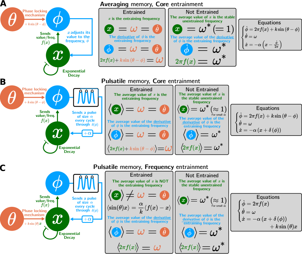
Figure S7: A), B) and C) provide intuitive pictures for, respectively, the averaging memory, core entrainment system, the pulsatile memory, core entrainment system, and the pulsatile memory, frequency entrainment system. For each system, a summary of some intuitive insights for both the entrained and not entrained cases is provided. Notice that B and C have the same "Not Entrained" panel.

Fig. S7 summarizes the different models presented in this paper and highlights some key analytical properties about them.