Phase-induced vortex pinning in rotating supersolid dipolar systems

Abstract

We analyze the pinning of vortices for a stationary rotating dipolar supersolid along the low-density paths between droplets as a function of the rotation frequency. We restrict ourselves to the stationary configurations of vortices with the same symmetry as that of the array of droplets. Our approach exploits the fact that the wave function of each droplet acquires a linear phase on the coordinates, and hence the relative phases between neighboring droplets allows us to predict the position of the vortices. For a confined system, the estimate accurately reproduces the Gross-Pitaevskii results in the spatial regions where the neighboring droplets are well defined.

I Introduction

Supersolids were experimentally created for the first time in 2017 in spin-orbit coupled Bose-Einstein condensates (BECs) [1], BECs with cavity mediated interactions [2, 3], and in 2019 in dipolar BECs [4, 5, 6], with many other experiments featuring them afterwards [7, 8, 9, 10, 11, 12, 13, 14, 15, 16, 17, 18, 19, 20]. This state of matter combines the frictionless flow of the superfluids with a translational symmetry breaking typical of crystals [21, 22, 23, 24, 25, 26]. In the case of dipolar supersolids, one can obtain them either by generating a roton instability into an already condensed gas [4, 5, 6, 27, 28, 18, 29, 30, 31, 32, 33], or by directly condensing the gas from a thermal cloud into a supersolid [20]. Dipolar supersolids break the translational symmetry by spontaneously forming a position-dependent density distribution, which includes droplets of high density separated by lower-density areas. In such a supersolid phase of dipolar BECs [34, 35, 36], given that droplets are separated by low density valleys, the barrier required for the nucleation of vortices is reduced with respect to the superfluid case (see e.g. [37]). In particular, for stationary rotating systems, it was shown that low-density regions reduce the energetic barrier for a vortex to enter the system, which lowers the nucleation frequency and help in pinning the vortices in the interstitial zones between droplets [35].

The aim of this work is to predict the positions of vortices in a stationary arrays in supersolid dipolar BEC [34, 35, 18] forming a triangular lattice of droplets when it is subject to rotation. Our approach consists in approximating the system wave function through a superposition of the localized wave functions of individual droplets. Such a hypothesis is based on the fact that the density is concentrated on the droplets, which are surrounded by very low relative density valleys. Then, any droplet exhibiting axial symmetry around a line parallel to the rotation axis acquires a homogeneous velocity field [38], which is determined by the velocity of the center of mass of the rotating droplet. In consequence, the phase of the droplet wave function turns out to exhibit a linear expression in terms of the spatial coordinates [38, 39]. Such an expression can be conveniently employed for estimating the vortex positions between two neighboring droplets through a simple formula, as it has been already shown for a BEC in rotating square lattices [39]. In the present work, which involves a triangular lattice, we show that the use of three droplets in the model leads to more accurate values for the vortex positions along the low-density paths that separate the droplets.

The paper is organized as follows. In Sec. II we introduce the basic characteristics and parameters of a rotating triangular lattice of droplets, which will be considered in our analysis, and in Sec. II.1 we outline the method for determining the vortex positions. In Sec. III we describe the confined system of dipolar atoms and show a typical stationary configuration, whereas Sec. III.1 is devoted to the determination of the coordinates of vortices of different configurations. Finally, a summary of the results is given in Sec. IV.

II Triangular droplet lattice

We start by considering the stationary configuration of a rotating supersolid dipolar BEC, which forms an extended triangular lattice of droplets. The key properties of this system are outlined below, and will be then used to predict the characteristics of the vortex array that emerges within the low-density regions between these droplets. We assume the density is modulated as [18]

$$\rho({\bf r})=\rho_{0}\,\left[1+C\,\sum_{i=1}^{3}\cos(\bm{q}_{i}\cdot\bm{r})\right],$$ (1)

where the parameter $C>0$ represents the contrast. The vectors $\bm{q}_{i}$, which lie in the $(x,y)$ plane, are defined by

$$\bm{q}_{1}=q\hat{y}\,,\,\,\bm{q}_{2}=-\frac{1}{2}q\hat{y}+\frac{\sqrt{3}}{2}q\hat{x}\,,\,\,\bm{q}_{3}=-\frac{1}{2}q\hat{y}-\frac{\sqrt{3}}{2}q\hat{x}\,,$$ (2)

with $q=2\pi/\lambda$. It is worth noting that in a realistic setup, the overall density factor may exhibit a dependence on the coordinate $z$, $\rho_{0}=\rho_{0}(z)$. This dependence can be modeled by a Gaussian or Thomas-Fermi distribution. However, for the purposes of the subsequent discussion, this dependency can be safely disregarded without loss of generality.

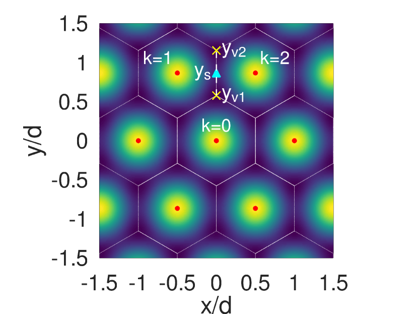
Figure 1: Density plot of the density distribution given by Eq. (1), where the density maxima are marked with red dots. The thin white lines indicate the low-density paths around the droplets, while the dashed line marks the specific path described in the text. In such a path, the saddle point at $y_{s}=\lambda$ is marked with a triangle, and the minima at $y_{v1}=d/\sqrt{3}$ and $y_{v2}=2d/\sqrt{3}$ (vertices) with crosses.

In Fig. 1 we show a plot of the density distribution in Eq. (1). By analyzing its maxima, minima, and saddle points, we can characterize the density pattern as follows. The distance between neighboring droplet maxima is $d=2\lambda/\sqrt{3}$. The minima are located at equidistant positions from three neighboring droplets, namely at the vertices of the hexagonal structure depicted in the figure. In the following, we will use the term path to denote the line segments connecting them (namely, each side of the hexagon). When the droplets have all the same size and shape, as in the ideal case depicted in Fig. 1, all paths in between the first ring of droplets are equivalent. These are the paths that will be specifically relevant for the discussion in Sec. III. Therefore, here we will focus ourselves on the vertical path marked by the dashed line in Fig. 1, without loss of generality. For this specific case, the two vertices are located along the $y$-axis at $y_{v1}=d/\sqrt{3}$ and $y_{v2}=2d/\sqrt{3}$. At the center of the path, $y_{s}=\sqrt{3}/2d$, which corresponds to the middle point between the two neighboring droplets, the density displays a saddle point.

When the supersolid lattice is put under rotation, stationary vortices will appear along the low-density paths between the droplets [39, 37, 33]. The position of the vortex along those paths, denoted as $Y_{v}$ for the specific path considered above, can be easily estimated using the ansatz discussed below, in Sec. II.1.

In Sec. III we will consider a finite realization of this system, which can be achieved through numerical calculations. In order to do so, we will introduce a harmonic trap to confine the system. Given that we also subject the system to rotation at constant frequency $\Omega$ along the $z$-axis, the effective confinement varies with $\Omega$. Then, the distribution of droplets and their densities vary as well. We will verify that a number of droplets arrange in a triangular lattice, and hence compute $d$ and the remaining geometrical quantities from the obtained densities for each frequency.

II.1 Estimate of the vortex positions

In this section, we outline the way to estimate the position of the vortices, following Ref. [39]. We assign to each droplet $k$ a localized wave function $w_{k}({\bm{r},\Omega})$ normalized to unity, where $\bm{r}=(x,y,z)$. Hence, the wave function of the system of droplets can be approximated by

$$\psi_{D}(\bm{r},t)=\sum_{k}w_{k}({\bm{r},\Omega})\,e^{i\phi_{k}(t)}\sqrt{N_{k}(t)}\,,$$ (3)

where ${N_{k}(t)}$ is the number of particles of the droplet, $\phi_{k}(t)$ its global phase, and the indices $k$ runs upon all the droplets. Given the axial symmetry of each droplet, we may further approximate [38]

$$w_{k}(\bm{r},\Omega)=|w_{k}(\bm{r},\Omega)|e^{i\frac{m}{\hbar}(\bm{r}-\bm{r}_{\text{cm}}^{k})\cdot(\bm{\Omega}\times\bm{r}_{\text{cm}}^{k})},$$ (4)

where we have fixed to zero the phase of $w_{k}$ at the center of mass of the droplet.

Two-droplet case. Let us first consider the case in which the vortex sits between two neighboring droplets, labeled as $k^{\prime}$ and $k$. Specifically, we examine the two droplets indicated in the upper section of Fig. 1, which are symmetric with respect to the vertical $y$-axis. We denote the generic coordinates of a vortex core in the $z=0$ plane as $(X_{v},Y_{v},0)$. Due to symmetry, a vortex lying between these two droplets will have $X_{v}=0$, while the vertical coordinate $Y_{v}$ can be obtained by requiring the vanishing of the wave function at the vortex core, $\psi_{D}(X_{v},Y_{v},0)=0$, namely

$$w_{k^{\prime}}(\bm{r})\,e^{i\phi_{k^{\prime}}}\sqrt{N_{k^{\prime}}}+w_{k}(\bm{r})\,e^{i\phi_{k}}\sqrt{N_{k}}=0\,,$$ (5)

where we have omitted the time dependence for ease of notation. By writing,

$$(\bm{r}-\bm{r}_{\text{cm}}^{k})\cdot(\bm{\Omega}\times\bm{r}_{\text{cm}}^{k})=(\bm{r}-\bm{r}_{\text{cm}}^{k^{\prime}})\cdot(\bm{\Omega}\times\bm{r}_{\text{cm}}^{k^{\prime}})\\ +\bm{r}\cdot(\bm{\Omega}\times(\bm{r}_{\text{cm}}^{k}-\bm{r}_{\text{cm}}^{k^{\prime}})),$$ (6)

Eq. (5) can be rewritten as,

$$\sqrt{N_{k}}|w_{k}|\,e^{i(\frac{m}{\hbar}\bm{r}\cdot(\bm{\Omega}\times(\bm{r}_{\text{cm}}^{k}-\bm{r}_{\text{cm}}^{k^{\prime}}))-\varphi_{k})}+\sqrt{N_{k^{\prime}}}|w_{k^{\prime}}|\,=0\,,$$ (7)

where $\varphi_{k}(t)=\phi_{k^{\prime}}(t)-\phi_{k}(t)$ is the phase difference between the centers of such neighboring droplets.

In terms of the center-of-mass coordinates one has,

$$\bm{r}\cdot(\bm{\Omega}\times(\bm{r}_{\text{cm}}^{k}-\bm{r}_{\text{cm}}^{k^{\prime}}))=-x(y^{k}_{\text{cm}}-y^{k^{\prime}}_{\text{cm}})\Omega\\ +y(x^{k}_{\text{cm}}-x^{k^{\prime}}_{\text{cm}})\Omega\,.$$ (8)

As for the droplet label $k$, here we set $k=0$ for the central droplet, and let run $k$ clockwise for the outer droplets, as indicated in Fig. 1. Then, considering the case of the two droplets with $k=2$ and $k^{\prime}=1$ in Eq. (8), for which $y^{1}_{\text{cm}}=y^{2}_{\text{cm}}$, we may obtain, from the condition that the imaginary and real parts of Eq. (7) should vanish, the vortex coordinate $Y_{v}(t)$,

$$Y_{v}(t)=\left(\frac{\varphi(t)}{\pi}+2l+1\right)\,\frac{\pi\hbar}{md\Omega}\,,$$ (9)

where $d=x^{2}_{\text{cm}}-x^{1}_{\text{cm}}$ is the distance between the center of mass of the droplets, and $\varphi=\varphi_{2}=\phi_{1}-\phi_{2}$. Here, $l$ is an integer number labeling different possible solutions, with $l=0$ corresponding to the first vortex that enters through that path [39]. It is also important to remark that the coordinates of the center of mass increase as functions of the rotation frequency due to the centrifugal force, and we will estimate its position by searching the density maxima of the droplets.

Three-droplet case. In principle, in a triangular lattice, when the location of a vortex approaches a vertex of the droplet lattice, the presence of a third neighboring droplet should affect the vortex position, and hence it becomes important to take such an effect into account. Then, one can approximate the wave function in such a region as

$$\psi_{D}(\bm{r},t)\simeq\sum_{k=0}^{2}|w_{k}(\bm{r},\Omega)|e^{i\frac{m}{\hbar}(\bm{r}-\bm{r}_{\text{cm}}^{k})\cdot(\bm{\Omega}\times\bm{r}_{\text{cm}}^{k})+i\phi_{k}}\sqrt{N_{k}}\,.$$ (10)

In this case we cannot extract an analytical expression for the vortex coordinates. However, by adequately modelling the individual wave functions of the droplets, an approximate solution can be obtained. Here we shall consider the two droplets at the first ring ($k=1,2$) together with the central one ($k=0$), a case that will be relevant for the finite realization presented in the following section. For such a purpose we will approximate $|w_{k}|$ by Gaussian functions with widths $a$ and heights which almost reproduce the characteristics of our droplets. We further assume that $\phi_{k}=\phi_{0}$ for all sites. With these approximations, we can again obtain an expression for $Y_{v}$ by imposing that the wave function of Eq. (10) vanishes at the position of the vortex core. In particular, the value of $Y_{v}$ is given by the solution of

$$\sqrt{\frac{N_{0}}{N_{1}}}\,e^{\dfrac{d(d-\sqrt{3}Y_{v})}{2a^{2}}}+2\cos\left(\frac{md}{2\hbar}\Omega Y_{v}\right)=0,$$ (11)

where we have accounted for the fact that in a finite realization the central droplet population $N_{0}$ may be different from the population $N_{1}=N_{2}$ of the other two droplets. Notice that Eq. (11) has multiple solutions which are related to those labeled by $l$ in Eq. (9).

The above Eq. (11), along with Eq. (9), constitutes one of the central results of the present work. In Sec. III.1, we will compare it with exact results from numerical simulations, demonstrating its accuracy in predicting vortex positions.

III Rotating stationary supersolid

In order to present a practical case study, we focus on investigating a rotating stationary supersolid configuration within a dipolar system akin to the one studied in Ref. [35]. Specifically, we consider a Bose gas composed by $N=1.1\times 10^{5}$ dipolar ¹⁶²Dy atoms trapped by an axially symmetric harmonic trap of frequencies $\{\omega_{r},\omega_{z}\}=2\pi\times\{60,120\}$ Hz. For this atomic species, the dipolar scattering length is $a_{dd}=130a_{0}$, where $a_{0}$ stands for Bohr radius. The magnetic dipoles are considered to be aligned along the $z$ direction by a magnetic field $\bm{B}$. The $s$-wave scattering length of the contact interaction is fixed to $a_{s}=92a_{0}$ throughout the whole paper. The system is set to rotate at an angular velocity $\Omega$ around the polarization axis.

The advantage of this specific configuration is that it features a triangular supersolid lattice as the ground state, which is the closest packing configuration and thus is of special interest. However, the model developed in this paper does not require any specific geometry and could be applied to other supersolid configurations as long as the positions of the droplets are correctly taken into account.

We consider the gas to be at $T=0$, thus no thermal fluctuations are taken into account. We describe the system using the usual extended Gross Pitaevskii (eGP) theory, which includes both the quantum fluctuations in the form of the Lee-Huang-Yang (LHY) correction [41, 42, 43] and the dipole-dipole interaction [44]. To account for the rotation of the condensate we will work in the rotating frame, for which an additional term is introduced into the energy functional [45, 46]. The energy functional of such a system can be written as $E_{\text{GP}}+E_{\text{dd}}+E_{\text{LHY}}+E_{\Omega}$, with

$$E_{\text{GP}} =\int\left[\frac{\hbar^{2}}{2m}|\nabla\psi(\bm{r})|^{2}+V(\bm{r})n(\bm{r})+\frac{g}{2}n^{2}(\bm{r})\right]d\bm{r}\,,$$

$$E_{\text{dd}} =\frac{C_{\text{dd}}}{2}\iint n(\bm{r})V_{\text{dd}}(\bm{r}-\bm{r}^{\prime})n(\bm{r}^{\prime})d\bm{r}d\bm{r}^{\prime}\,,$$

$$E_{\text{LHY}} =\frac{2}{5}\gamma_{\text{LHY}}\int n^{5/2}(\bm{r})d\bm{r}\,,$$ (12)

$$E_{\Omega} =-\Omega\int\psi^{*}(\bm{r})\hat{L}_{z}\psi(\bm{r})d\bm{r}\,,$$

where $E_{\text{GP}}=E_{\text{k}}+E_{\text{ho}}+E_{\text{\text{int}}}$ is the standard GP energy functional including the kinetic, potential, and contact interaction terms, $V(\bm{r})=(m/2)\sum_{\alpha=x,y,z}\omega_{\alpha}^{2}r_{\alpha}^{2}$ is the harmonic trapping potential, and $g=4\pi\hbar^{2}a_{s}/m$ is the contact interaction strength. The system wave function $\psi(\bm{r})$ is normalized to the total number of particles $N$ and the condensate density is given by $n(\bm{r})=|\psi(\bm{r})|^{2}$. The inter-particle dipole-dipole potential is $V_{\text{dd}}(\bm{r})=(1-3\cos^{2}\theta)/(4\pi r^{3})$ with $C_{\text{dd}}\equiv\mu_{0}\mu^{2}$ its strength, $\mu$ the modulus of the dipole moment $\bm{\mu}$, $\bm{r}$ the distance between the dipoles, and $\theta$ the angle between the vector $\bm{r}$ and the dipole axis, $\cos\theta=\bm{\mu}\cdot\bm{r}/(\mu r)$. The LHY coefficient is $\gamma_{\text{LHY}}={128\sqrt{\pi}}{\hbar^{2}a_{s}^{5/2}}/(3m)\left(1+3\epsilon_{\text{dd}}^{2}/2\right)$, with $\epsilon_{\text{dd}}=\mu_{0}\mu^{2}N/(3g)$. The last term $E_{\Omega}$ accounts for the rotating frame, with $\hat{L}_{z}=-i\hbar(x\partial_{y}-y\partial_{x})$ representing the angular momentum operator along $z$. To obtain the supersolid stationary states in the rotating frame, we perform numerical simulations in which we minimize the above energy functional employing a conjugate gradient method (see e.g. [48]). Among the several possible stationary configurations, we select those corresponding to a triangular supersolid lattice by means of a suitable choice of the trial wave function .

         

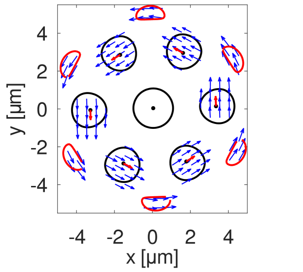
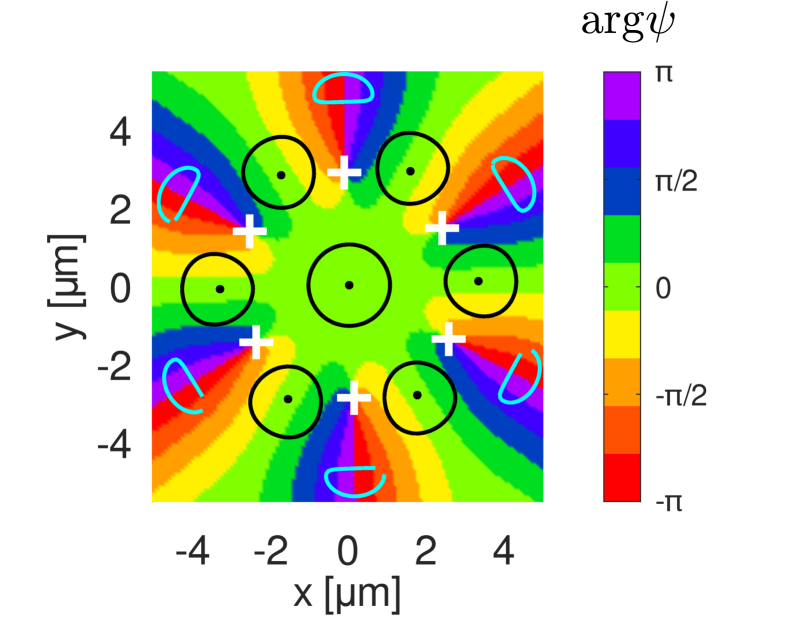
Figure 2: Typical density and phase configuration of the stationary supersolid triangular lattice obtained from the eGP simulations, in the rotating frame. Here $\Omega=2\pi\times 20$ Hz. (top) Isodensity contours and velocity field around the stationary droplets. The black curves correspond to the contours around the six first-ring droplets at a density value of $0.2\rho_{\text{max}}$, and the red curves around the low-density clouds at a density value of $0.04\rho_{\text{max}}$, where $\rho_{\text{max}}$ is the maximum density value. The red arrows at the droplet maxima correspond to the $\bm{v}_{k}$. (bottom) Color map of the phase of the supersolid wave function at the plane $z=0$. The plus signs mark the location of the vortices, and the curves are isodensity contours of the droplets for the same values as in the top panel.

A typical configuration is displayed in Fig. 2, featuring the density contours and velocity field in the upper panel, and the phase distribution along with the position of the vortex cores in the lower panel. This figure corresponds to the case with $\Omega=2\pi\times 20$ Hz, and serves as a representative illustration for all cases within the range of rotation frequencies considered in this work. Figure 2 reveals well-localized, circularly symmetric densities of the gas droplets (depicted in black) arranged in a triangular structure formed by a central droplet at $(x,y)=(0,0)$, and six droplets located along a ring around it. It may be seen that each of these droplets exhibits a uniform velocity field $\bm{v}_{k}=\bm{\Omega}\times\bm{r}^{k}_{\text{cm}}$. Additionally, at the border, very low-density clouds with non-circular shapes (in red) are present and display a diffuse distribution with an extended velocity field. Then, such a cloud is not included in the region where $\psi_{D}$ is defined. Between the droplets, we observe the presence of vortices whose positions form a lattice structure determined by the periodic arrangement of the supersolid droplets, see bottom panel in Fig. 2.

III.1 Vortex pinning

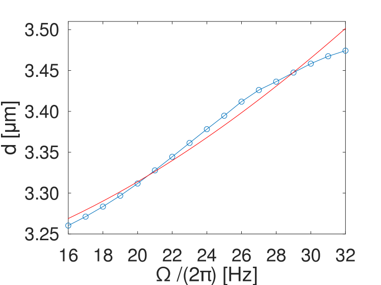
Figure 3: Mean value of the inter-droplet distance $d$ (blue circles) as a function of the rotation frequency $\Omega$. The data have been obtained by identifying the density maxima from the calculated supersolid configurations. The solid red line correspond to the distance for a non-rotating configuration with an effective trap frequency $\tilde{\omega}_{r}=\sqrt{\omega_{r}^{2}-\Omega^{2}}$.

In order to investigate the position of the vortices as a function of the rotation, we employ the method outlined in Sec. II.1. Here we focus on the location of the vortices along the low-density paths bounded by two vertices, such as the line joining $y_{v1}$ and $y_{v2}$ in Fig. 1. We begin by considering the effect of pairs of neighboring droplets. The mean relative distance $d$ between droplet pairs is shown in Fig. 3 as a function of the rotation frequency $\Omega$ (blue circles). We observe an increase of such a distance with the frequency, which can be mainly attributed to the effect of the centrifugal force acting on the particles. This can be proved by comparison with the inter-droplet distance of a non-rotating gas trapped at the effective frequency $\tilde{\omega}_{r}=\sqrt{\omega_{r}^{2}-\Omega^{2}}$ so as to mimic the centrifugal force effect, shown in the same Fig. 3 (solid red line).

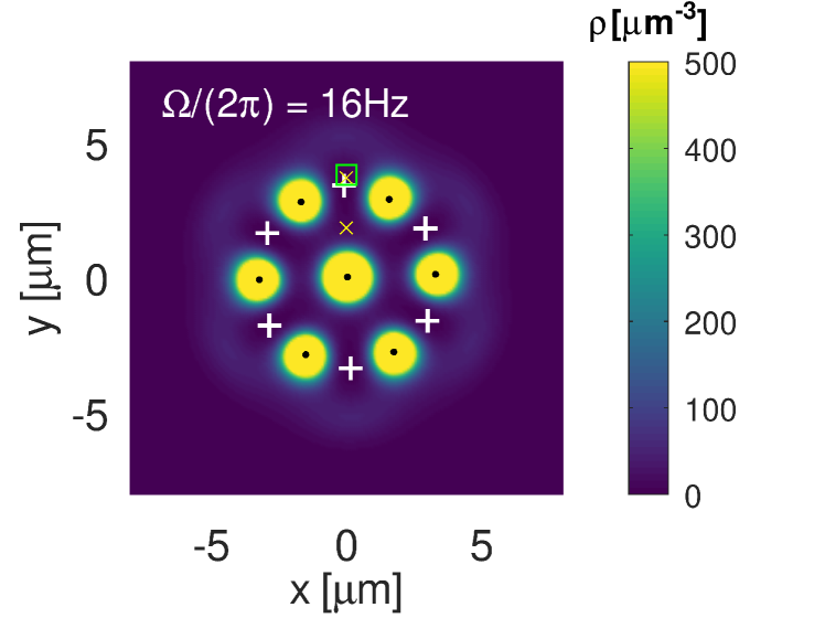
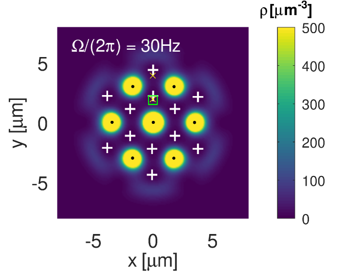
Figure 4: Density plots of stationary supersolid configurations obtained from the eGP simulations at the $z=0$ plane for some representative rotation frequencies: $\Omega/(2\pi)=16,\,20,$ and $30$ Hz (from top to bottom, respectively). The black dots mark the maxima of the density. The vortex positions determined with the plaquette method are shown as white plus symbols ($+$). The position of the vortex core obtained from the analytical ansatz, along the straight path between the vertices $y_{v1}$ and $y_{v2}$ [yellow crosses ($\times$)], is indicated by a green square.

Then, we extract the positions of any vortices present in the system using a plaquette method [50] and compare them to our estimate in Eq. (9). In Fig. 4 we show examples of the stationary density distribution at different rotation frequencies, along with the vortex locations. This figure shows that the vortices are not necessarily pinned to the vertices, but rather along the low-density paths that connect them. The configurations conserve the triangular symmetry both for the density and phase profiles, and we observe that they display vanishing phase differences among droplet centers, i.e., $\varphi_{k}=0,\forall k$. This leads to the prediction $Y_{v}=(2l+1)\pi\hbar/(md\Omega)$. It is worth noting that the position of the vortex along the straight path between the vertices $y_{v1}$ and $y_{v2}$ (see figure) corresponds to the solution with $l=0$, whereas different values of $l$ identify additional vortices that may enter the system from outside. Nevertheless, we remark that those additional vortices that appear, e.g., for $\Omega/(2\pi)=30$ Hz (bottom panel of Fig. 4) cannot be properly described by the ansätze (9) and (11) because they are nucleated in the low-density cloud, outside the region of validity of the analytical approach.

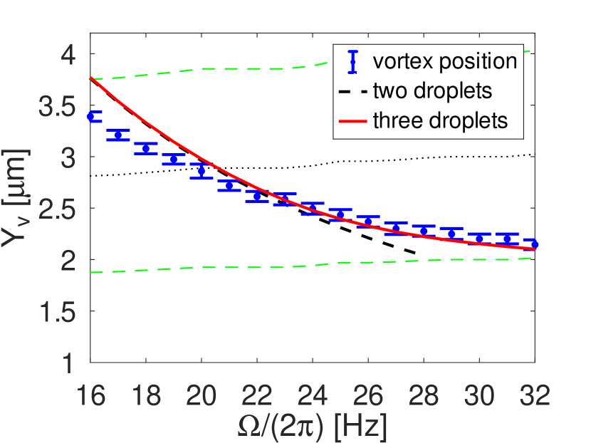
Figure 5: Vortex position as a function of the rotation frequency $\Omega$, for the stationary configurations. The positions extracted from full eGP simulations using a plaquette method (see text) are marked as blue points with their corresponding error bar. The prediction provided by Eq. (9) with $l=0$ (black dashed line) and (11) (solid red line) have been calculated using the values of $d$ obtained from the numerical simulations, which are shown in Fig. 3. They correspond to the ansatz based on two and three droplets, respectively. The parameters of the three-droplet ansatz are $a=0.75\mu$m and $\sqrt{N_{0}/N_{1}}=1.06$. The (green) dashed lines represent positions of the vertices, whereas the (black) dotted line indicates the position of the saddle point.

At this point, we are now able to compare the analytical predictions of Eqs. (9) and (11) with the extracted values of the vortex positions $Y_{v}$ as a function of the rotating frequency, as summarized in Fig. 5. Overall, this figure demonstrates that the analytical ansatz discussed in Sec. II.1 provides an accurate prediction for the positions of the vortex cores between supersolid droplets in stationary rotating configurations. It is also worth noting that the pinning at the saddle points, represented by a dotted line in the graph, and density minima do not seem to be favored with respect to other points along such paths, as stated previously (see e.g. [33]). Instead, the vortex position smoothly changes as a function of the rotation frequency. As a matter of fact, in a rotating supersolid, the slow variation of the vortex location arises from the imprinted velocity field on the droplets, rather than from density holes that typically pin vortices in non-rotating systems.

Finally, let us comment about the two- and three-droplet approximations. Although the two-droplet ansatz is not expected to hold far from the saddle point, where other effects should be taken into account, the ansatz accurately predicts the rotation frequency at which vortices locate near such a point, through an analytical formula. Instead, the three-droplet model permits us to numerically estimate with accuracy the position of vortices along the line joining the saddle point and the vertex $y_{v1}$. This is evident from the figure, where the positions of the vertices are indicated by (green) dashed lines. In particular, for the saddle point $y_{s}$, the prediction of the rotation frequency for reaching such a point using the two- and three-droplet approximations differ in less than 0.3%, as the exponential term in Eq. (11) is smaller than $10^{-2}$ at the saddle point. Notice that neglecting such an exponential term altogether, the two-droplet ansatz is exactly recovered. In contrast, for the vertex $y_{v1}$, the two-droplet rotation frequency estimate is given by $\Omega/2\pi={\hbar\sqrt{3}}/{(2md^{2})}\simeq 28$ Hz; whereas, using the three-droplet approach of Eq. (11), one obtains $\Omega/2\pi\simeq 37$ Hz. This result may be seen considering that the argument of the exponential vanishes at the vertex $y_{v1}$, and hence the frequency at which the vortex should reach such a vertex satisfies

$$\cos\left(\frac{md^{2}\Omega}{2\hbar\sqrt{3}}\right)=-\frac{1}{2}\sqrt{\frac{N_{1}}{N_{0}}}.$$ (13)

Then, assuming equal populations $N_{0}=N_{1}$ the above equation leads to $\Omega/2\pi=2\hbar/(\sqrt{3}md^{2})\simeq 37$ Hz for the lowest $\Omega$ value that corresponds to vortex position with $l=0$ in Eq. (9), consistently with the numerical findings of the eGP simulations. In summary, we have shown that the three-droplet model better describes the vortex position as a function of rotation frequency from the saddle $y_{s}$ to vertex $y_{v1}$.

IV Summary and concluding remarks

We have shown that when a dipolar supersolid is subjected to rotation, the positions of vortices between two neighboring droplets can be predicted in terms of the rotation frequency and the inter-droplet distance. Such a distance can be roughly estimated using the non-rotating system with a harmonic potential that mimics the net confinement produced by the rotating trap. The vortex positions are a smooth function of the rotation frequency and are distributed along the low-density paths between both droplets, instead of being fixed at a density minimum. Such a formulation applies in the regions where robust droplets acquire on-site axially symmetric profiles. We have further shown that a very accurate value of the vortex locations can be numerically obtained by considering three neighboring droplets within the triangular lattice. In the present case, due to the external confinement, three well-formed neighboring droplets could be observed only around the first vertex, but given that our estimate remains valid from the vertex up to the saddle, we may conclude that the model should work well for less confined systems where more droplets are formed around other vertices of the triangular lattice.

As a final remark, the approach can be generalized to more complex droplets configurations as long as the droplets themselves are axially symmetric and well defined. Vortices will likely be placed in areas in which 2 or 3 neighboring droplets are enough to precisely predict their positions, regardless of the lattice structure of the supersolid.