Energy stable gradient flow schemes for shape and topology optimization in Navier-Stokes flows††thanks: This work was supported in part by the National Key Basic Research Program under grant 2022YFA1004402, the Science and Technology Commission of Shanghai Municipality (No. 22ZR1421900 and 22DZ2229014), and the National Natural Science Foundation of China under grant (No. 12071149).
Abstract
We study topology optimization governed by the incompressible Navier-Stokes flows using a phase field model. Novel stabilized semi-implicit schemes for the gradient flows of Allen-Cahn and Cahn-Hilliard types are proposed for solving the resulting optimal control problem. Unconditional energy stability is shown for the gradient flow schemes in continuous and discrete spaces. Numerical experiments of computational fluid dynamics in 2d and 3d show the effectiveness and robustness of the optimization algorithms proposed.
Keywords: Topology optimization, incompressible Navier-Stokes equations, stabilized gradient flow, energy stability, phase field method
1 Introduction
Shape and topology optimization [1] of computational fluid dynamics is a popular topic with applications such as auto-coronary bypass anastomoses in medical science [2], the laminar flow wing design in aeronautics [3] and pipe flow [4]. Such optimal control problems in fluid flow [3] aim to seek a configuration or layout for optimizing some objective (e.g., energy dissipation and geometric inverse problem) subject to geometric and physical constraints such as incompressible fluid flows [5, 6, 7, 8, 9, 10, 11] or compressible Navier-Stokes equations [12]. Compared to shape optimization by adjusting the profile of geometric boundary to obtain better configuration [13], topology optimization can perform both shape and topological changes of structures. Numerical realization of topology optimization in fluid flows can be performed via the variable density method [14], topological derivative [15], level set method [16], phase field method [17, 18], etc.
As diffusive interface tracking techniques, the phase field method [18, 19, 20, 21, 22] is introduced for minimizing general volume and surface functionals constrained by incompressible Navier-Stokes flows. The porous medium approach [14] proposed by Borrvall and Petersson enables the governing equations to be defined on a fixed domain with a variable linear term characterizing the permeability. The main idea of the phase field model of topology optimization is to combine both objective and so-called Ginzburg–Landau energy to construct the total free energy. The latter is a diffuse interface approximation of perimeter regularization implying the existence of the optimal control problem [20]. For topology optimization constrained by Navier-Stokes flow, Garcke et al. [21, 18] discussed the differentiability of the solution to the phase field function, the first-order necessary condition from sensitivity analysis, and sharp interfacial asymptotic analysis.
The gradient flow method actually was a powerful tool for minimization of nonlinear or multi-physical coupling type of energy functional for many problems (see, e.g., [23, 24]). From the numerical perspective, a gradient flow scheme is generally evaluated on the energy dissipation and its computational efficiency [23]. The energy dissipative gradient flow scheme is of crucial importance to topology optimization implying that the sequence generated by the algorithm is convergent and monotonous. Unlike phase field models in the physical background such as interface dynamics [19] or crystallization [25], the difficulty of constructing an energy dissipative gradient flow scheme for topology optimization arises from the coupling among the gradient flow, linear/nonlinear physical constraints of partial differential equations and possible extra adjoint systems. For shape design constrained by Stokes flow in the phase field model, an energy monotonic-decaying gradient flow scheme is proposed [17, 26] for minimization of energy dissipation via the stabilized method. An efficient iterative thresholding method [27, 28] was developed for topology optimization for Stokes and the Navier–Stokes flow. To the best of our knowledge, however, there exists no research work on energy dissipative gradient flow schemes for topology optimization constrained by the nonlinear partial differential equations such as the incompressible Navier-Stokes flow.
In this paper, we derive the gradient flow of the phase field model for topology optimization of incompressible Navier-Stokes flow and prove the energy dissipation property in continuous space by overcoming the introduction of the extra adjoint variables that are induced by nonlinear constraints. Then we propose energy dissipative gradient flow schemes (Allen-Cahn and Cahn-Hilliard types) based on the so-called stabilization method [29, 30] by adding stabilization terms to avoid strict time step constraints, which treats the nonlinear terms explicitly and the linear terms implicitly. For the Navier-Stokes flows by the porous medium approach, the Fréchet differentiability of state functions with respect to phase field function [21] defines the unique solution of linearized Navier-Stokes equation. The uniform boundedness of the velocity field and pressure function is also guaranteed. These analysis results motivate us to deduce the Lipschitz continuity of the solution to the phase field function which is of use in showing energy dissipation of the gradient flow. We note that the unconditional energy stability holds when the stabilized coefficients are larger than the coefficients depending on Lipschiz conditions, uniform bounds of the solution, and geometric area.
The rest of the paper is organized as follows: In section 2, we briefly introduce the phase field model and the governing steady-state Navier-Stokes equations. Then the topology optimization is built. The uniform boundedness of the solution pairs and adjoint variables are shown by the assumption that the gradient of velocity is smaller than a prescribed constant depending on the viscous coefficient and geometric measure. In section 3, we proposed the generalized gradient flow schemes first to solve the topology optimization problem. The energy dissipation of the gradient flow in continuous space is addressed by combining both state and adjoint variables which is an important clue for the stability of the scheme in time discretization. Then the Lipschtiz continuity of both state and adjoint variables is shown via the error estimate analysis and Sobolev compact embedding Theorem. After that, we present the main Theorem to show the stabilized gradient flow schemes are unconditional energy stable for both Allen-Cahn and Chan-Hilliard types. We also prove the cut-off technique does not affect the monotonicity of the cost functional by gradient flow scheme. In section 4, we introduce the conforming mixed finite element method to discretize the state variables (velocity field, pressure function) as well as the adjoint variables. The algorithm with a stable semi-implicit scheme is proposed to evolve the phase field function numerically. Various numerical experiments in 2D and 3D have been tested to verify the effectiveness of the algorithms proposed. Section 4 draws brief conclusions and some potential values to generalize such gradient flow schemes to other topology optimization.
2 Model problem
In this section, we introduce the phase field model for shape and topology optimization in a viscous incompressible fluid. The purpose of shape and topology optimization here is to seek an optimized configuration attaining the minimization of a given cost functional (typically dissipated energy) subject to stationary incompressible Navier-Stokes equations and some geometric constraint.
Let be an open bounded domain with Lipschitz continuous boundary . The whole domain is partitioned into three disjoint subregions where , and represent the fluid region, solid region and diffuse layer, respectively. The boundary is partitioned into both nonoverlapping Dirichlet and Neumann boundaries with (see Fig. 1 left), where consists of the inlet as well as the wall, and represents the outlet. First, we introduce notations involving Sobolev spaces [31]. Let be a Lebesgue space of square-integrable functions on . Denote with being the generalized derivative of with respect to . Denote and . Then denote the vectorial function spaces , with its dual space , and . Denote Sobolev space with divergence-free constraint . Let us use a same notation to define inner products of type by and for any scalar functions and vectorial functions . The phase field function can be seen as a “density” function (see Fig. 1 right) such that
| (1) |
2.1 Governing equations
Let the positive number be the viscous coefficient. Define the following bilinear form and trilinear form , respectively
where the vectorial functions are given by , and , respectively. We refer to [32, Lemma IX.1.1 and Lemma IX.2.1] and [33] for some useful properties on the trilinear form.
Lemma 2.1.
The trilinear form is well-defined and continuous in the space . The following estimate holds
| (2) |
where
with being the Lebesgue measure of . Furthermore, the following properties hold:
| (3) | ||||||
The permeability function for medium [21, page 225] is non-negative with satisfying
| (4) | ||||
Let the Cauchy stress tensor be with being an identity tensor. Let be a prescribed velocity field imposed on the inlet and the wall. Define the Sobolev spaces and for state and adjoint variables. Consider a weak formulation of a steady-state incompressible Navier-Stokes equation: find such that
| (5) |
where is a given source. The existence of (5) is valid (see [18, Lemma 2.7]) for every phase field function with a.e. in . The uniqueness [18, Lemma 2.8] of (5) holds by the assumption that .
2.2 Phase-field model
The shape functional with specific purpose is defined by the phase field function and the velocity field where the non-negative integrand is Fréchet differentiable with respect to and . Consider the shape functional of energy dissipation . Let be the volume of the solid region. The double well potential [34, page 421]
| (6) |
has the formulation with uniform upper bound of its derivative. Next, we can construct the total free energy by the summation of the Ginzburg-Landau energy, the shape functional and the least square of volume error as
| (7) |
where represents the thickness of the diffuse layer, and . Then the shape and topology optimization problem is to seek such that
| (8) |
where is the solution of (5) with given phase field function . The existence of the minimizer for optimal control problem (8) holds by using the lower semi-continuity of the objective functional and some compactness properties (see [21, 18]). We introduce the following adjoint equations corresponding to the optimization problem (8).
Lemma 2.2.
Let domain be an open bounded domain. Suppose that is differentiable with respect to with the Fréchet derivative denoted as . Then the weak form of the adjoint problem (a generalized Stokes equation) satisfies: find such that
| (9) |
where the directional derivative for energy dissipation.
Proof.
By utilizing the weak formulation of (5), define the following functional
| (10) |
The Lagrange functional is introduced associated with total free energy and (10)
| (11) |
Then the constrained problem can be transformed into the saddle point problem [35]
| (12) |
By the Karusch-Kuhn-Tucker condition, the saddle point of is characterized by
| (13) | ||||||
The first line in (13) implies the adjoint equations while the second line in (13) leads to the steady-state incompressible Navier-Stokes equations. ∎
The following analysis is based on the assumption that the boundary condition of the velocity field is the homogeneous Dirichlet condition.
Lemma 2.3.
Proof.
We refer to [18, Lemma 2.8] where the existence and uniqueness results for the Navier-Stokes equations (5) are discussed requiring that . The uniform boundedness (14) of the solution pair for Navier-Stokes equations (5) independent of phase field function is proved referring to [21, Lemma 4.3]. For the adjoint equations (9) of the general cost functional, the solvability and uniqueness has also been discussed referring to [21, Lemma 4.9] requiring . We are going to show the uniform boundedness of the adjoint variables by assuming which is of help to the following estimate. Let the test function in (9) so that for . After applying Lemma 2.1, Cauchy inequality and Poincaré inequality, we obtain
| (16) | ||||
which implies that
| (17) |
Furthermore by [36, Lemma II.2.1.1], we obtain unique such that
| (18) |
is fulfilled for some constant . ∎
3 Gradient flow
In this section, we construct an efficient and effective method to solve the optimal control problem (8) numerically. The minimum can be found by introducing the gradient flow with a virtual temporal dimension. The phase field function is extended to where is the prescribed terminal time. Given free energy functional bounded from below, denote its variational derivative as . The general form of the gradient flow [23] can be written as
| (19) |
supplemented with suitable boundary conditions. The nonpositive symmetric operator is the dissipation mechanism including the gradient flow of Allen-Cahn type with and the gradient flow of Cahn-Hilliard type with (the Laplacian). Since the gradient flow preserves mass conservation, hence no extra volumetric constraint needs to be introduced. To simplify the presentation, we assume throughout the paper that the boundary conditions are chosen such that all boundary terms will vanish when integration by parts is performed. The gradient flow for solving the optimal control problem (8) reads: find such that
| (20) |
Lemma 3.1.
Proof.
The existence of variational derivative and hold for all by the implicit Theorem [21] implying that
| (22) |
By the chain rule of variational differentiation, we obtain
| (23) | ||||
Taking the test function with in adjoint equations (9), we have
| (24) |
Combing (22), (23) and (24) yields
| (25) |
which allows the conclusion to hold. ∎
Proposition 3.2.
Under the gradient flow (20), the energy stable holds for all such that
| (26) |
Proof.
Take the differentiation of the total energy in (7) with respect to the temporal variable yielding that
| (27) |
where the derivative denotes . Next for the last term in (27), we obtain
| (28) |
according to the chain rule in differentiation . After using the adjoint equations (9) with test functions , we have
| (29) |
Differentiate (5) with respect to to derive
| (30) |
Combining (28) - (30), we obtain
| (31) |
By using the integration by parts and combining (20), (27) and (31), we obtain (26) thanks to the nonnegative operator of . ∎
Now, we are going to construct the energy dissipative gradient flow scheme for solving the optimal control problem (8). Let and denote a time partition with time step size for . For simplicity, consider a uniform time discretization with , where the number of time levels . The first-order semi-implicit scheme with generalized stabilization of gradient flow (20) reads
| (32) |
where the nonlinear term
and the general stabilization operator denotes with each . Then we begin to prove the property of the unconditional energy stable for the semi-implicit scheme (32). For proving the unconditional energy stability of the scheme (32), we need to verify the Lipschtiz boundedness of state and adjoint variables with respect to the phase field function
Lemma 3.3.
Let be given such that . Suppose that is Lipschitz continuous with respect to its argument: For any , there exists positive coefficient independent of satisfying that
| (33) |
Suppose that and are the solution of Navier-Stokes equations (5), respectively. Then the following estimate holds for state variables
| (34) |
where . Furthermore, if and are the solution of adjoint equations (9), respectively. Then the following estimates hold for adjoint variables
| (35) |
where
| (36) |
with being a constant related to the Poincaré inequality.
Proof.
Let and be the solution pairs of Navier-Stokes equations (5), respectively. Then the substraction together with setting the test function yields that
| (37) | ||||
For , we have . After applying Lemma 2.1, Cauchy inequality, Hölder equality, and Poincaré inequality, we obtain
| (38) | ||||
where the Sobolev imbedding Theorem is used for ignoring its constant and depends on the Poincaré inequality. After that, we can deduce the following estimate
| (39) |
Let and are the solution pairs of adjoint equations (9). The substraction by setting the test function yields that
| (40) | ||||
By the rearrangement of the trilinear terms, we obtain
| (41) | ||||
For , we have . Similarly applying Lemma 2.1, Cauchy inequality, Hölder equality and Poincaré inequality, we obtain
| (42) | ||||
yielding
| (43) | ||||
where the Sobolev imbedding Theorem is used for . The boundedness result can be further deduced by
| (44) | ||||
where the estimate (34) is used. ∎
Next, the estimate of the adjacent cost functionals is discussed.
Lemma 3.4.
Suppose that the phase field function is evolved by the scheme (32).
Proof.
By the identity, it holds for all
| (47) |
yielding that
| (48) | ||||
For last two terms in the last equation of (48), we have
| (49) | ||||
Given , take the test functions in (9) yielding that
| (50) |
Considering the Navier-Stokes equations (5) with two consecutive time steps, then the substraction leads to
| (51) |
where we have taken the test functions by . For the nonlinear terms in (51), we have
| (52) | ||||
where the residual is second-order term of the substraction . Similarly, we have
| (53) | ||||
where the residual is . Thus from (50) to (53), we obtain
| (54) | ||||
We are prepared to deduce the property of unconditional energy stable with semi-implicit gradient flow scheme.
Theorem 3.5.
Let are positive values independent of such that
| (55) |
The unconditional energy stable holds for the stabilized gradient flow scheme (32)
| (56) |
Proof.
The residue terms in (45) can be bounded by Lemma 3.3
| (57) | ||||
and
| (58) | ||||
The subtraction between adjacent Ginzburg-Landau energy gives
| (59) | ||||
where we use Taylor expansion up to the second order by taking . Then use the linear property of the volume functional and apply the Cauchy-Schwarz inequality to obtain
| (60) | ||||
We conduct the estimation via Lemma 3.4 and (59)
| (61) | ||||
and
| (62) | ||||
thanks to the nonnegative operator and sufficient large values and . ∎
Remark 3.6.
The popular method to construct an energy stable scheme of gradient flow is the class of convex splitting method [37] involving inner iteration. While it requires updating P.D.E. repeatedly for each time step in the case of topology optimization. The stabilization treats the nonlinear terms explicitly and adds a stabilization term to avoid strict time step constraints [29]. In our case, the instability factors come from the nonlinear term in Navier-Stokes equations and the introduction of adjoint variables. The other method to construct the energy stable scheme is introducing a scalar auxiliary variable (see [23]). However, such a method can only keep the energy stability of the modified energy instead of the original energy.
Then we introduce the bounded value function space
| (63) |
and the corresponding projection operator defines
| (64) | ||||
Modify the volume function and to obtain the following result.
Lemma 3.7.
Proof.
The projection operator satisfies . Then using the definition of the permeability function defined on the whole domain and the volume function, it holds
| (66) | ||||
such that is the solution pair of (5). Let be partitioned into two disjoint domains where
| (67) |
Then we obtain
| (68) | ||||
where vanishes on for is a.e. constant. Furthermore, by the nonnegativity of the double well potential, we have
| (69) | ||||
where vanishes on for takes value on 0 or 1. The invariant of the permeability function and volume function under the projection leads to
| (70) |
and
| (71) |
Combining (68) (69) (70) and (71), we conclude the estimate. ∎
Remark 1.
Given the previous phase field function , then compute the velocity field via the Navier-Stokes equations. After that update the phase field function via the stabilized gradient flow (32) and then compute the corresponding velocity field . In this way, the minimizing sequence is generated by repeating the above procedure. From Theorem 3.5, the sequence satisfies the energy dissipation
which guarantees the convergence and monotonicity. However, the phase field function may exceed the range causing inaccuracy in computing the Navier-Stokes equations.
Another way to construct the convergent sequence meanwhile keeping phase field function in the range is computing by (32), (5) and (9) first. Then use the projection on phase field function to obtain . We note that is still the solution pair of the Navier-Stokes equations (5) because the permeability function does not change by the projection operator. Then, use the stabilized gradient flow to obtain the next decreasing iteration
Finally, we alternatively take the projection step and the stabilized gradient flow step to generate the sequence such that
which preserves the energy dissipation and bounds the phase field function in .
4 Numerical realization
In this section, we introduce the finite element to discretize the Navier-Stokes equations (5), the adjoint equation (9) and the gradient flow (32) of the phase field.
4.1 Finite element discretization
Consider a family of unstructured meshes satisfying the union of triangular units , where the mesh size is with being the diameter of any . Let us consider the conforming finite element subspaces characterized as the discrete velocity function space and the discrete pressure function as well as the phase field function space . We shall also admit a compatibility condition [38, 39, 40] between the discrete velocity and pressure spaces and by assuming that there exists a positive constant such that
| (72) |
Denote the space of bubble functions by , where the bubble function and are the barycentric coordinates of . Then the MINI (-bubble/) element [38, 39] for discretization of Navier-Stokes equations is given by
The following subspaces are necessary to describe the Dirichlet boundary condition for the velocity field and for the adjoint function . The phase field function is discretized in piece-wise linear function space . The discrete variational problem of Navier-Stokes equations (5) reads: find such that
| (73) |
Similarly, the discrete problem of adjoint equations (9) reads: find such that
| (74) |
The discrete variational problem of gradient flow (32) is given by: find such that
| (75) |
where is the discrete nonpositive symmetric operator such as the discrete Laplacian for gradient flow and the identity operator for gradient flow . For Allen-Cahn gradient flow, take the test function in the second equation of (75) then insert it into the first equation to simplify the expression. Hence no intermediate variable is introduced. Since the stability proofs of stabilized semi-implicit schemes (32) are all variational, they can be directly extended to fully discrete stabilized semi-implicit schemes with mixed finite element methods.
Theorem 4.1.
Proof.
Replace the continuous variables with the discrete variables as well as for the adjoint variables (). Then follow the procedure of Theorem 3.5 to obtain the conclusion. ∎
To verify the monotonic-decaying property of the projection in the fully-discrete sense, we refer to [17, Lemma 4.1] with the phase field function discretized by the piecewise linear finite element method
| (77) |
where defines the corresponding discrete projection operator
| (78) | ||||
Denote the discrete permeability . Then the following monitonicity property holds.
Lemma 4.2.
The Lagrange multiplier is introduced to further eliminate the volume error for the Allen-Cahn gradient flow. Furthermore, the nonlinear term can be expressed by
| (80) |
where is the weighted parameter, is the normalized factor. For updating the Lagrange multiplier, a Uzawa type scheme reads
| (81) |
Note that the discrete Navier-Stokes system in (73) has a nonlinear convection term. A typically efficient Newton scheme preserving locally quadratic convergence rate is proposed by solving numerically a series of Oseen problems: Given for the previous approximation, find such that
| (82) |
Then the approximate solution pair is updated by In this section, we propose a topology optimization algorithm based on the scheme (75). We use the trick that once the state and adjoint variables are solved, the phase field is evolved via the gradient flow scheme for several steps to further improve the efficiency. Now, we are prepared to present Algorithm 1 (Allen-Cahn) and Algorithm 2 (Cahn-Hilliard) for topology optimization using the semi-implicit gradient flow scheme. We note that the projection can not be used in the Cahn-Hilliard gradient for it may break the mass conservation.
4.2 Numerical experiments
Numerical simulations are performed with FreeFem++ [41]. All numerical results are performed on a computer with 12th Gen Intel(R) Core(TM) i7-12700 2.10 GHz and 16 GB memory. Set where the permeability coefficient for the following Examples.
Example 1 (Diffuser in 2d): Consider a benchmark of the shape design for the diffuser in 2d space (see [14]). The computational domain is set to be a square (see Fig. 2 left). The flow on the inlet is imposed by the prescribed function . The volume target is set to be of the solid phase. The basic parameters are given as follows: and . Set for Allen-Cahn flow and for Cahn-Hilliard flow. Choose the initial phase field function be the constant .
-
•
Test the performance of stabilized Allen-Cahn gradient flow by Algorithm 1 for realizing the topology optimization. No stabilized terms and projection operator are used for the Allen-Cahn gradient flow in situation 1. Set for situation 2, for situation 3, and as well as the projection operator for situation 4. The maximum and minimum of the phase field function are presented in Table 1 during shape evolution showing that the stabilized Allen-Cahn gradient flow with the projection operator behaves well even in large time step (see optimal shape in Fig. 5 right). Then fix , and . The optimal shapes and the corresponding velocity fields are shown in Fig. 4 with different viscous parameters. The curves of convergence histories for total energy and volume errors are presented in Fig. 3 demonstrating the property of energy decreasing and the high accuracy of volume control.
-
•
Next, consider algorithm 2 by the Cahn-Hilliard gradient flow for topology optimization. Choose and for the stabilized parameters. Though the Cahn-Hilliard gradient flow has the property of mass conservation, we note that the mass of solid region is not equivalent to volume function in which the phase field function may exceed the range . The stabilized parameters are well chosen such that the phase field function is well controlled in the range during shape evolution (see Table 2) to meet the demand of volume constraint. The optimal shapes are shown in Fig. 5 (left and middle) with different viscous parameters. The convergence histories of total energy and mass variation are shown in Fig. 6 showing that the Chan-Hiliard gradient flow scheme proposed has the energy dissipation property.
| Situation 1 | Situation 2 | Situation 3 | Situation 4 | |||||
|---|---|---|---|---|---|---|---|---|
| iter | ||||||||
| 0 | 0.5 | 0.5 | 0.5 | 0.5 | 0.5 | 0.5 | 0.5 | 0.5 |
| 1 | 1e73 | -1e76 | 1.22 | 0.51 | 0.86 | 0.54 | 0.89 | 0.54 |
| 20 | - | - | 1.46 | 0.24 | 1.37 | -0.06 | 1.00 | 0.00 |
| 40 | - | - | 1.38 | -0.01 | 1.36 | -0.03 | 1.00 | 0.00 |
| 60 | - | - | 1.35 | 0.00 | 1.34 | -0.02 | 1.00 | 0.00 |
| 80 | - | - | 1.39 | 0.00 | 1.34 | -0.01 | 1.00 | 0.00 |
| 100 | - | - | 1.40 | 0.00 | 1.33 | -0.01 | 1.00 | 0.00 |
| iter | iter | ||||||||
|---|---|---|---|---|---|---|---|---|---|
| 0 | 0.65 | 0.65 | 0.65 | 0.65 | 0 | 0.65 | 0.65 | 0.65 | 0.65 |
| 20 | 0.67 | 0.63 | 0.78 | 0.55 | 20 | 0.67 | 0.63 | 0.77 | 0.55 |
| 40 | 1.03 | -0.04 | 1.02 | -0.02 | 40 | 1.03 | -0.02 | 1.02 | -0.02 |
| 60 | 1.00 | -0.06 | 1.03 | -0.03 | 60 | 1.00 | -0.06 | 1.03 | -0.03 |
| 80 | 1.01 | -0.05 | 1.03 | -0.03 | 80 | 1.01 | -0.05 | 1.03 | -0.03 |
| 100 | 1.01 | -0.05 | 1.03 | -0.03 | 100 | 1.01 | -0.05 | 1.03 | -0.03 |
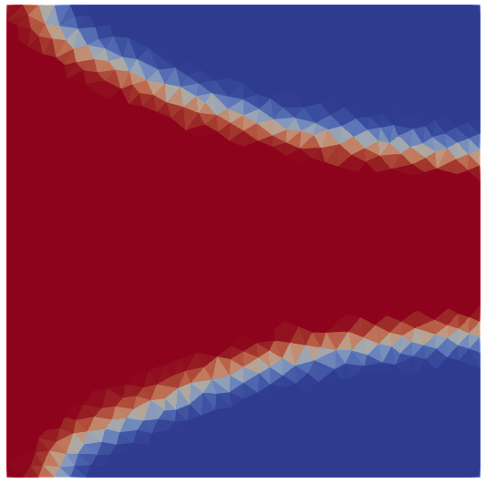
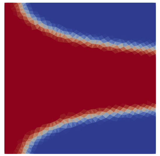
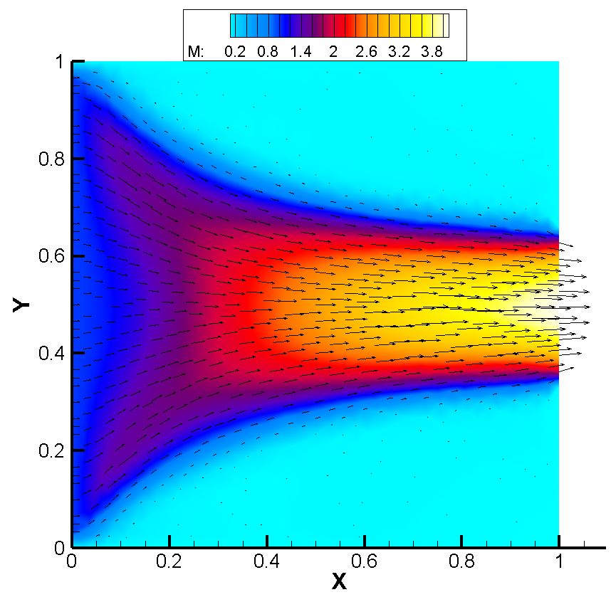
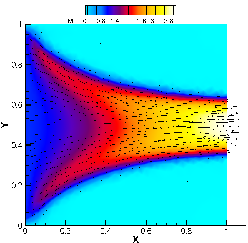

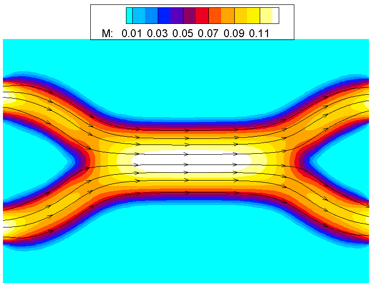
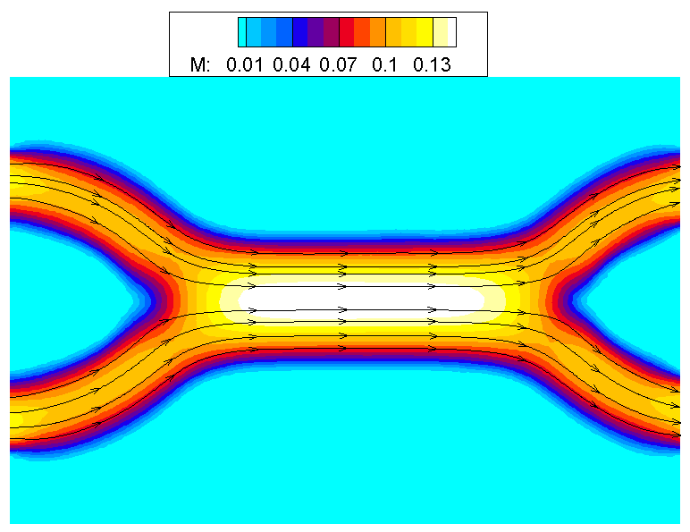
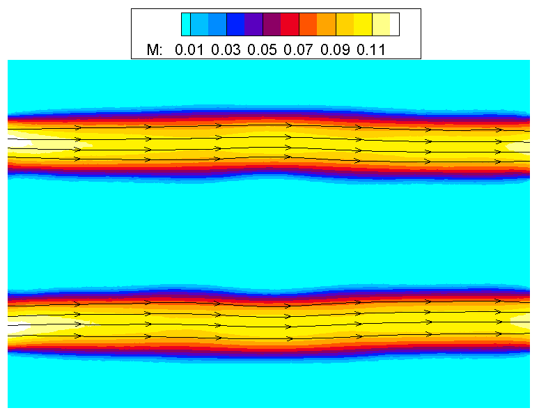
Example 2 (Bypass design): The second Example is the shape design for the bypass in 2d space. The computational domain is set to be a rectangle (see Fig. 2 right) with two inlets and two outlets. The flow on the inlet is imposed by the prescribed function .
-
•
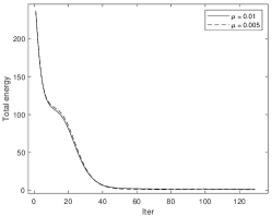
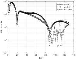
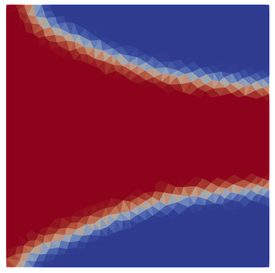
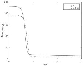
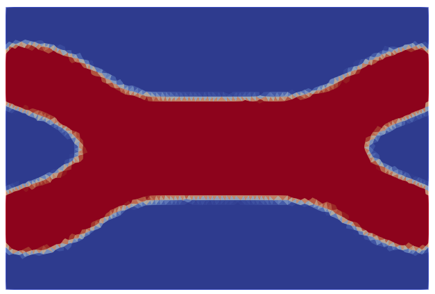
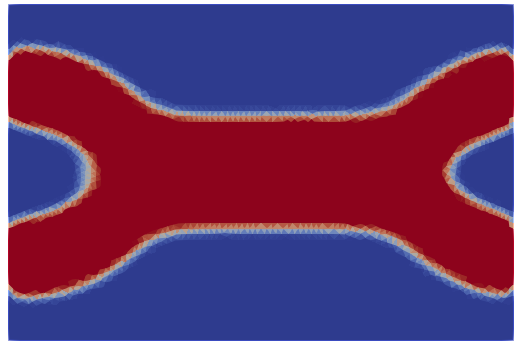
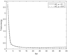
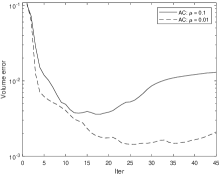
At first, fix the volume target in which the solid phase occupies almost the volume of the whole domain. Consider the algorithm 1 with the projected Allen-Cahn gradient flow scheme to evolve the phase field function. The basic parameters are given as follows: and . The initial phase field function is . The optimal distribution with single connected shape and the corresponding velocity fields are presented on the left and middle of Fig. 7 where the viscous coefficients and . The convergence histories of total energy are shown in Fig. 8 left demonstrating that the algorithm 1 has the energy dissipative property. Meanwhile, the volume error (Fig. 8 right) is well controlled almost by .
-
•
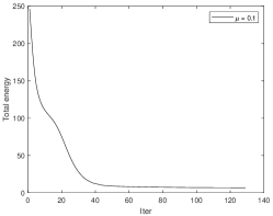
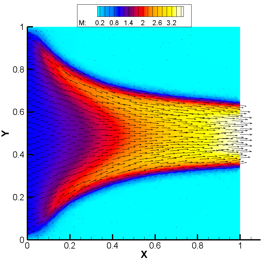
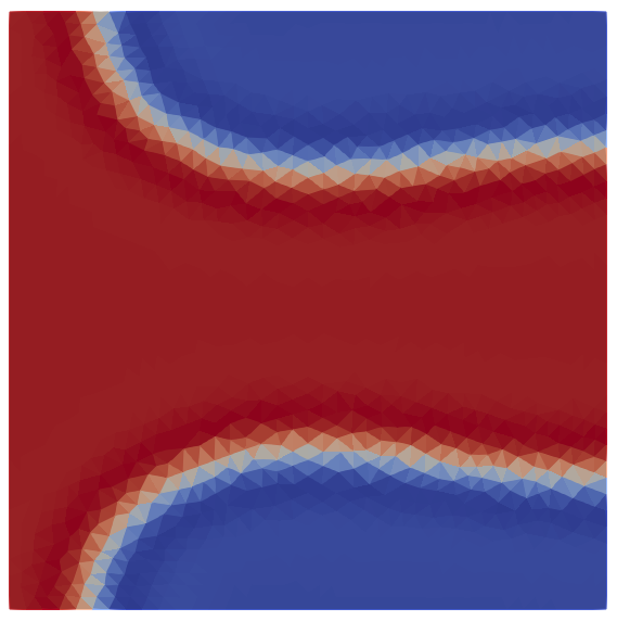
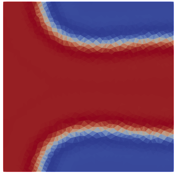
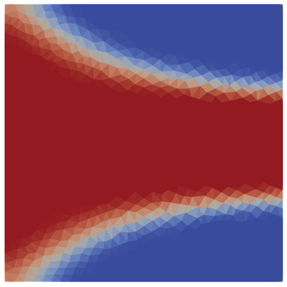
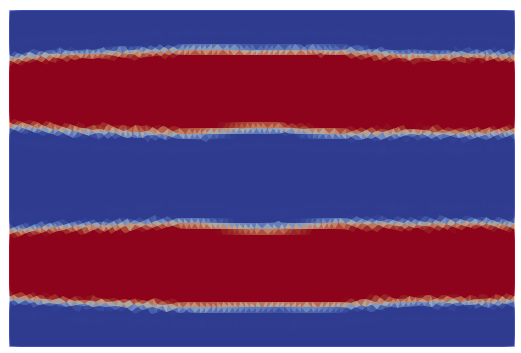
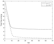
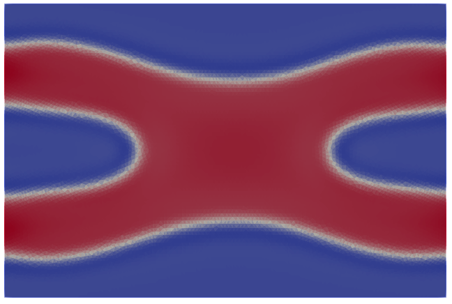
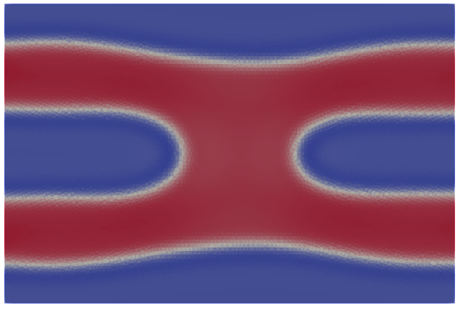
Consider the Cahn-Hilliard gradient flow algorithm 2 for topology optimization. Choose the initial phase field function . The basic parameters are given as follows: and . The other conditions are the same as the above. The optimal distribution and its corresponding velocity field exhibit the double channels in Fig. 7 right. The convergence histories of total energy is presented in the middle of Fig. 8 showing the effectiveness of the algorithm 2. Furthermore, different (see Fig. 9) have been tested to display the optimal configurations and curves of total free energy.

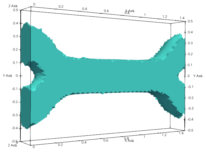
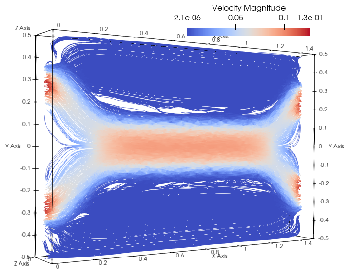
Example 3 (Bypass design in 3d): This example is solved by Algorithm 1. See Fig. 10 for the domains to design the internal flow channels.
-
•
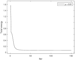
(A). The design domain is the Fig. 10 left. The velocity on the inlet is . Set the volume target 0.85 for the solid phase. The basic parameters are given as follows: and =10. The optimal distribution from two directions and corresponding velocity fields are displayed in Fig. 11 with different viscous coefficients. The curves of convergence histories for both total energy and volume in Fig. 12 shows the energy dissipative for the scheme in 3d space.
-
•
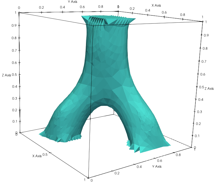
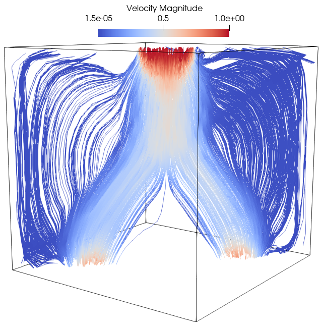
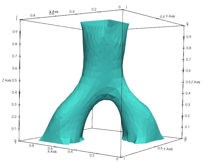
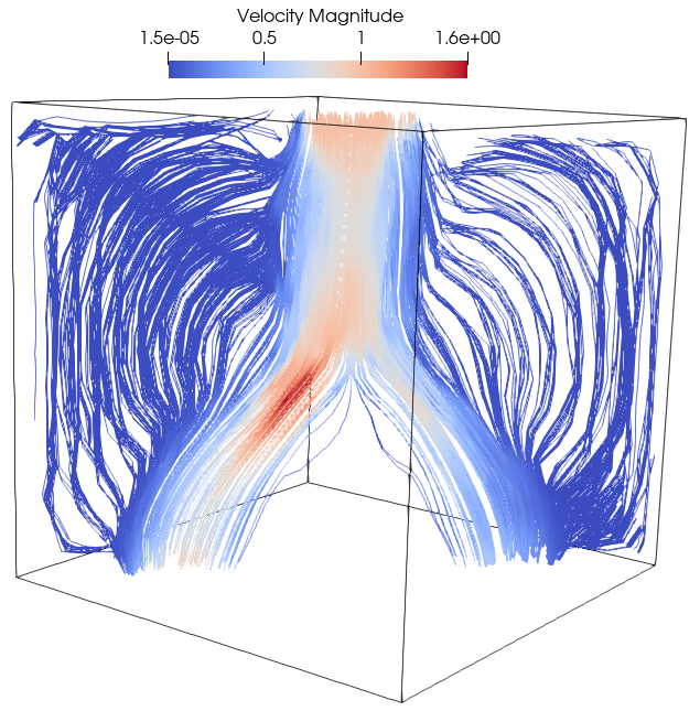
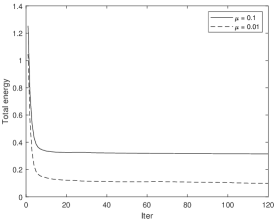
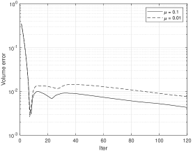
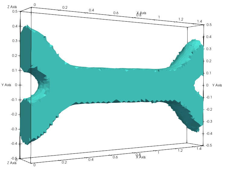
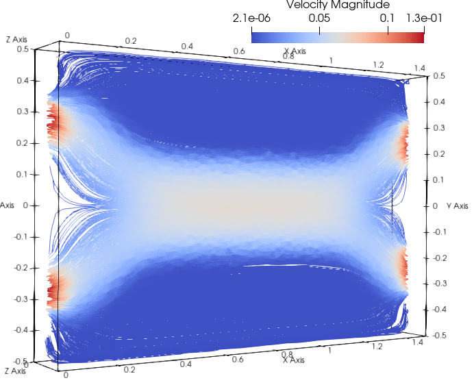
(B). The design domain is the Fig. 10 right. The velocity on the inlet is . The basic parameters are given as follows: , , and . The optimal distribution from two directions and corresponding velocity fields are displayed in Fig. 13 with different viscous coefficients. The curves of convergence histories for both total energy and volume in Fig. 14 shows the energy dissipative for the scheme in 3d space.


5 Conclusion
Topology optimization in incompressible Navier-Stokes equations has been considered using a phase field model. We propose the novel stabilized semi-implicit schemes of the gradient flow in Allen-Cahn and Cahn-Hilliard types for solving the resulting optimal control problem. The unconditional energy stability is shown for the gradient flow schemes in both continuous and discrete spaces by the Lipschtiz continuity. Numerical examples of computational fluid dynamics show effectiveness and robustness of the optimization algorithm proposed. The stabilized gradient flow scheme is the constant coefficient equation that can be solved efficiently. The scheme keeping energy dissipation is simple to realize and may can be extended to other topology optimization models with general objective functionals such as geometric inverse problems or with nonlinear physical constraints.
References
- [1] M.P. Bendsøe and O. Sigmund, Topology Optimization. Theory, Methods and Applications, Springer-Verlag, Berlin, 2003.
- [2] A. Quarteroni, L. Dede, A. Manzoni, and C. Vergara, Mathematical Modelling of the Human Cardiovascular System: Data, Numerical Approximation, Clinical Applications, Cambridge University Press, Cambridge, 2019.
- [3] B. Mohammadi and O. Pironneau, Applied Shape Optimization for Fluids, Clarendon Press, Oxford, 2001.
- [4] C. Dapogny, P. Frey, and F. Omnès et al. Geometrical shape optimization in fluid mechanics using FreeFem++, Struct. Multidisc. Optim., 58 (2018), pp. 2761–2788.
- [5] I. P. A. Papadopoulos and P. E. Farrell, Preconditioners for computing multiple solutions in three-dimensional fluid topology optimization, SIAM J. Sci. Comput., 45 (2023), pp. B853-B883.
- [6] I. P. A. Papadopoulos, P. E. Farrell, and T. M. Surowiec, Computing multiple solutions of topology optimization problems, SIAM J. Sci. Comput., 43 (2021), pp. A1555-A1582.
- [7] J. Li and S. Zhu, Shape optimization of Navier–Stokes flows by a two-grid method, Comput. Methods Appl. Mech. Engrg., 400 (2022), 115531.
- [8] Y. Deng, Z. Liu, J. Wu, and Y. Wu, Topology optimization of steady Navier–Stokes flow with body force, Comput. Methods Appl. Mech. Engrg., 255 (2013), pp. 306–321
- [9] A. Gersborg-Hansen, O. Sigmund, and R. B. Haber, Topology optimization of channel flow problems, Struct. Multidiscip. Optim., 30 (2005), pp. 181–192,
- [10] J. Li, S. Zhu and X. Shen, On mixed finite element approximations of shape gradients in shape optimization with the Navier-Stokes equation, Numer. Methods Partial Differential Equations, 39 (2023), 1604-1634.
- [11] S. Schmidt and V. Schulz, Shape derivatives for general objective functions and the incompressible Navier-Stokes equations, Control Cybernet., 39 (3) (2010), pp. 677-713.
- [12] P. Plotnikov and J. Sokołowski, Compressible Navier-Stokes Equations. Theory and Shape optimization, Basel: Springer-Verlag, 2012.
- [13] W. Gong, J. Li, and S. Zhu, Improved discrete boundary type shape gradients for PDE-constrained shape optimization, SIAMJ. Sci. Comput., 44 (2022), pp. A2464-A2505.
- [14] T. Borrvall and J. Petersson, Topology optimization of fluid in Stokes flow, Internat. J. Numer. Methods Fluids, 41 (2003), pp. 77–107.
- [15] P. Guillaume and K. Sid Idris, Topological sensitivity and shape optimization for the Stokes equations, SIAM J. Control Optim., 43 (2004), pp. 1-31.
- [16] S. Zhou and Q. Li, A variational level set method for the topology optimization of steady-state Navier-Stokes flow, J. Comput. Phys., 227 (2008), pp. 10178-10195.
- [17] F. Li and J. Yang, A provably efficient monotonic-decreasing algorithm for shape optimization in Stokes flows by phase-field approaches, Comput. Methods Appl. Mech. Engrg., 398 (2022), 115195.
- [18] H. Garcke and C. Hecht, Applying a phase field approach for shape optimization of a stationary Navier-Stokes flow, ESAIM Control Optim. Calc. Var., 22, (2016), pp. 309-337.
- [19] D. Anderson, G. McFadden, and A. Wheeler, Diffuse-interface methods in fluid mechanics, Annu. Rev. Fluid Mech., 30 (1998), pp. 139–165.
- [20] H. Garcke, C. Hecht, M. Hinze, and C. Kahle, Numerical approximation of phase field based shape and topology optimization for fluids, SIAM J. Sci. Comput., 37 (2015), pp. A1846-A1871.
- [21] H. Garcke, C. Hecht, M. Hinze, C. Kahle, and K. Lam, Shape optimization for surface functionals in Navier-Stokes flow using a phase field approach, Interfaces Free Bound., 18 (2016), pp. 219–261.
- [22] B. Jin, J. Li, Y. Xu and S. Zhu, An adaptive phase-field method for structural topology optimization, J. Comput. Phys., 506 (2024), 112932.
- [23] J. Shen, J. Xu and J. Yang, a new class of efficient and robust energy stable schemes for gradient flows, SIAM Rev., 61 (2019) pp. 474-506.
- [24] Q. Du and X. B. Feng, The phase field method for geometric moving interfaces and their numerical approximations, in Geometric Partial Differential Equations, Part I, Handb. Numer. Anal., 21 (2020), pp. 425-508.
- [25] K. Elder, M. Katakowski, M. Haataja, and M. Grant, Modeling elasticity in crystal growth, Phys. Rev. Lett., 88 (2002), 245701.
- [26] Y. Li, K. Wang, Q. Yu, Q. Xia and J. Kim, Unconditionally energy stable schemes for fluid-based topology optimization, Commun. Nonlinear Sci. Numer. Simul., 111 (2022), 106433.
- [27] H. Leng, D. Wang, H. Chen, and X. Wang, An Iterative thresholding method for topology optimization for the Navier–Stokes flow, ICIAM 2019 SEMA SIMAI Springer Ser., 1 (2022) 205–226.
- [28] H. Chen, H. Leng, D. Wang, and X. Wang, An efficient threshold dynamics method for topology optimization for fluids, CSIAM Trans. Appl. Math., 3 (2022), pp. 25-56.
- [29] J. Zhu, L. Chen, J. Shen, and V. Tikare, Coarsening kinetics from a variable mobility Cahn-Hilliard equation—application of semi-implicit Fourier spectral method, Phys. Rev. E., 60 (1999), pp. 3564–3572.
- [30] J. Shen and X. Yang, Numerical approximations of Allen-Cahn and Cahn-Hilliard equations, Discrete Contin. Dyn. Syst., 28 (2010), pp. 1669-1691.
- [31] R. Adams and J. Fournier. Sobolev Spaces. Elsevier, 2003.
- [32] G. O. Galdi, An Introduction to the Mathematical Theory of the Navier–Stokes Equations, Springer, New York, 2011.
- [33] E. Casas, M. Mateos, and J.P. Raymond, Error estimates for the numerical approximation of a distributed control problem for the steady-state Navier–Stokes equations, SIAM J. Control Optim., 46 (2007), pp. 952-982.
- [34] Y. Cai, H. Choi and J. Shen, Error estimates for time discretizations of Cahn-Hilliard and Allen-Cahn phase-field models for two-phase incompressible flows. Numer. Math., 137 (2017), pp. 417-449.
- [35] M. C. Delfour and J.-P. Zolésio, Shapes and Geometries: Metrics, Analysis, Differential Calculus, and Optimization. 2nd ed., SIAM, Philadelphia, 2011.
- [36] H. Sohr, The Navier-Stokes Equations: An Elementary Functional Analytic Approach. Birkhäuser Advanced Texts, Springer Verlag, 2001.
- [37] D. J. Eyre, Unconditionally gradient stable time marching the Cahn-Hilliard equation, in MRS Proc. 529, Cambridge University Press, 1998.
- [38] F. Brezzi and M. Fortin, Mixed and Hybrid Finite Element Methods, Springer, New York, 1991.
- [39] V. Girault and P.A. Raviart, Finite Element Methods for Navier-Stokes Equations: Theory and Algorithms, Springer-Verlag, Berlin, 1986.
- [40] R. Temam, Navier-Stokes Equations: Theory and Numerical Analysis, American Mathematical Soc., 2001.
- [41] F. Hecht, New development in FreeFem++, J. Numer. Math., 20 (2012), pp. 251-265.