Chemistry Beyond Exact Solutions on a Quantum-Centric Supercomputer
A universal quantum computer can be used as a simulator capable of predicting properties of diverse quantum systems [1]. Electronic structure problems in chemistry offer practical use cases around the hundred-qubit mark [2]. This appears promising since current quantum processors have reached these sizes. However, mapping these use cases onto quantum computers yields deep circuits, and for for pre-fault-tolerant quantum processors, the large number of measurements to estimate molecular energies leads to prohibitive runtimes [3]. As a result, realistic chemistry is out of reach of current quantum computers in isolation. A natural question is whether classical distributed computation can relieve quantum processors from parsing all but a core, intrinsically quantum component of a chemistry workflow. Here, we incorporate quantum computations of chemistry in a quantum-centric supercomputing architecture, using up to 6400 nodes of the supercomputer Fugaku to assist a Heron superconducting quantum processor. We simulate the N2 triple bond breaking in a correlation-consistent cc-pVDZ basis set, and the active-space electronic structure of [2Fe–2S] and [4Fe–4S] clusters [4], using 58, 45 and 77 qubits respectively, with quantum circuits of up to 10570 (3590 2-qubit) quantum gates. We obtain our results using a class of quantum circuits that approximates molecular eigenstates, and a hybrid estimator. The estimator processes quantum samples, produces upper bounds to the ground-state energy and wavefunctions supported on a polynomial number of states. This guarantees an unconditional quality metric for quantum advantage, certifiable by classical computers at polynomial cost. For current error rates, our results show that classical distributed computing coupled to quantum processors can produce good approximate solutions for practical problems beyond sizes amenable to exact diagonalization.
The most common task in theoretical quantum chemistry is the computation of ground-state energies by solving the Schrödinger equation in the Born-Oppenheimer approximation. Exact numerical solutions in a finite basis set have a cost growing combinatorially in the number of electrons and orbitals. This limits exact diagonalization in the full configuration interaction (FCI) to system sizes close to 22 electrons in 22 orbitals (22e,22o) [5] and (26e,23o) [6]. For system sizes beyond the reach of FCI, one must rely on approximate methods, e.g., diagrammatic techniques, wavefunction ansatzes, and Monte Carlo integration [7, 8].
Progress in quantum computing has triggered a flurry of theoretical proposals for computational chemistry over the last decade (e.g., [9, 10, 11]). At the same time, attempts have been made at implementations on pre-fault-tolerant quantum processors [12, 13, 14, 15, 16, 17, 18], but these have so far been limited to small systems, for two main reasons. First, despite numerous efforts to improve on the measurement problem (e.g., [19, 20, 21]), runtime for energy expectation value estimation on interesting systems remains out of any reasonable timescale. Second, the depths of chemically-motivated quantum circuits for computations of chemistry are very high. For unitary coupled cluster [22] and a single step of time evolution, these quantities scale as [23] on a system with spin-orbitals. While this scaling can be improved with various techniques [24], on pre-fault-tolerant devices the signal emerging from circuits of such size is weakened by the accumulation of gate errors and qubit decoherence.
I Methods
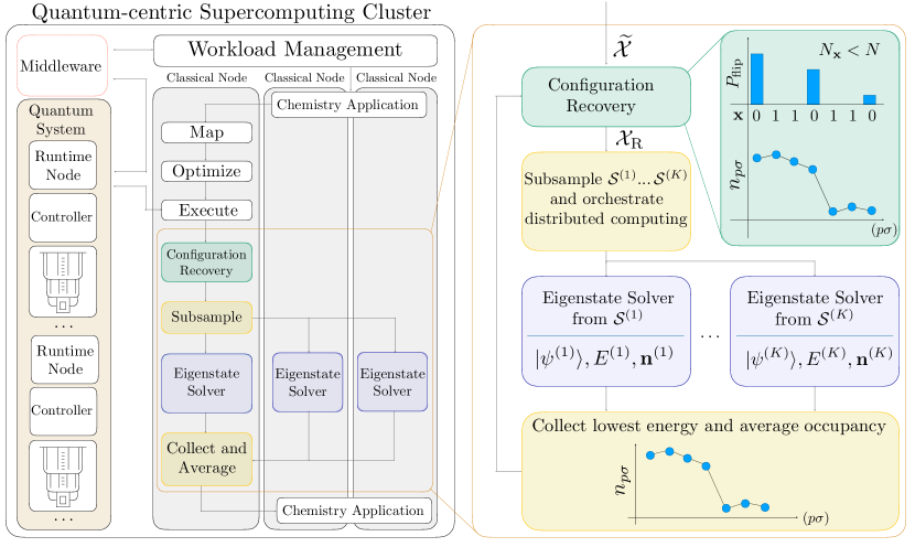
We set up the discussion of our results by considering the quantum-centric supercomputing architecture [25] schematized in Fig. 1 a . The architecture enables scaling of computational capacity by leveraging quantum processors for their natural task: executing a limited number of large quantum circuits. We follow the workflow in Fig. 1 to summarize our methods.
Our main goal is to find the ground state of chemistry Hamiltonians
| (1) |
expanded over a discrete basis set. Here we have defined the fermionic creation/annihilation operator / associated to the -th basis set element and the spin , while and are the one- and two-body electronic integrals, obtained from standard chemistry software [26]. Throughout this manuscript we use molecular orbitals as basis set elements. We map the degrees of freedom of Eq. (1) to qubits with a Jordan-Wigner (JW) transformation [27]. We then construct a quantum circuit to be executed on quantum hardware, preparing a state on qubits, which represents a molecular wavefunction on molecular spin-orbitals. In the JW mapping, the single-qubit basis states / represent empty/occupied spin-orbitals. These mapping and optimization steps are performed on classical nodes, see Fig. 1. We execute the circuit on a quantum computer and measure in the computational basis. Repeating this produces a set of measurement outcomes
| (2) |
in the form of bitstrings distributed according to some ; the bitstrings represent electronic configurations (Slater determinants).
On a pre-fault-tolerant quantum computer, the action of noise alters the distribution from its ideal form to some other , which generates the noisy set of configurations , accessible to us via quantum measurement. Noise in the quantum system broadens the distribution over configurations that do not contribute to low-energy states, so-called deadwood [28]. As a result, only a fraction of contains a meaningful quantum signal. To improve this scenario, we introduce a probabilistic self-consistent configuration recovery technique, which allows a probabilistic partial recovery of noiseless configuration samples from .
The configuration recovery scheme is inspired by the structure of chemistry problems. The Hamiltonian in Eq. (1) conserves the number of particles separately for each spin species. The recovery routine targets configurations that have the wrong particle number due to the accumulation of errors in the execution of the quantum circuit.
Repeated rounds of recovery can be carried out self-consistently. The first step of each recovery round is to iterate through the set and find configurations with particles. If (or ), bits are sampled to be flipped from the set of occupied (or empty) spin-orbitals, according to a distribution proportional to a monotonically-increasing function [29] of , the distance from the current value of the bit to the average occupancy of the spin-orbital , obtained from the previous recovery round. This generates a new set of recovered configurations .
Following the next step of Fig. 1, we build batches of configurations using samples from the set , according to a distribution proportional to the empirical frequencies of each in . We project and diagonalize the Hamiltonian over each , as proposed recently in the quantum selected configuration interaction method [30, 31], which draws inspiration from the classical selected configuration interaction framework [32, 33, 34, 35, 36, 37, 38].
Each batch of sampled configurations spans a subspace in which the many-body Hamiltonian is projected:
| (3) |
The ground states and energies of , which we label and , are then computed using the iterative Davidson method on multiple classical nodes. The computational cost – both quantum and classical – to produce is polynomial in , the dimension of the subspace.
The ground states are then used to obtain new occupancies
| (4) |
for each spin-orbital tuple , averaged on the batches. These occupancies are sent back to the configuration recovery step, and this entire self-consistent iteration is repeated until convergence. The initial guess for used for the first round of recovery comes from the raw quantum samples in the correct particle sector. The configuration recovery routine can be seen effectively as a problem-informed clustering of a noisy signal around the occupations .
Let us now discuss the advantages and limitations of the method. First, on a noiseless signal , it is guaranteed to succeed efficiently if the ground state has a support of polynomial size, and if the wavefunction prepared on the quantum processor has a support similar to that of the ground state. In general, independently of the wavefunction support size, one can unambiguously benchmark by comparing with other methods that can only produce upper bounds to the ground state energy. In this regard, our method shares the same working assumptions as classical CI methods. Within the CI framework, quantum computing will allow us to test the performance of unitary circuits that are hard to simulate classically [39].
To establish some insight on the configuration recovery, we analytically compute a lower bound on the probability of recovering electronic configurations that have been corrupted by noise, as a function of their Hamming distance from an integer rounding of , using a global depolarizing noise model , where is the parameter that controls the amount of noiseless quantum signal [29]. We find that the likelihood of recovery decays exponentially with the system size and also with the Hamming distance from the configuration that best approximates . Since classical CI methods also require exponential time to reach configurations with high Hamming distances from a reference state, it would be possible for the quantum-centric architecture presented here to perform a more efficient simulation at some finite system size and error rates.
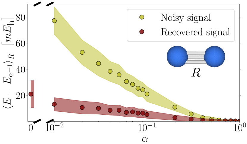
To further test noise robustness, we perform numerical simulations that confirm the improvements of applying the configuration recovery routine to the dissociation of N2 (6-31G basis set). In this test we sample from the exact ground state and we set a subspace dimension of .
Fig. 2 shows the error in the ground-state energy relative to the noiseless case (), as a function of the amount of signal , for the estimator both with and without configuration recovery. On the N2 model, errors below can be obtained from signal using the raw noisy samples. However, by using configuration recovery we can tolerate a signal to reach the same error. This numerical experiment hints that the use of configuration recovery will be crucial for large-scale experiments.
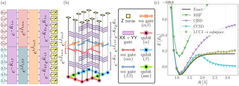
Before presenting our experimental results, we discuss the circuits used to produce the candidate ground states. We employ a truncated version of the local unitary cluster Jastrow (LUCJ) ansatz [40], shown in Fig. 3 (a),
| (5) |
Here are generic one-body operators, are density-density operators restricted to spin-orbitals that are mapped onto adjacent qubits [40], and is the bitstring representing the restricted Hartree-Fock (RHF) state in the JW mapping. Through this local approximation, the LUCJ ansatz allows for moderate circuit depths. Its accuracy derives from the connection with unitary coupled cluster theory and adiabatic state preparation [41, 39, 40]. The moderate depths of LUCJ are due to the use of exponentials of one-body operators, implementable in linear depth and a quadratic number of 2-qubit gates, and density-density operators, implementable in constant depth and a linear number of ZZ rotations (due to the locality approximation) [40]. The LUCJ circuit, compiled into one- and two-qubit gates, is shown in Fig. 3 (b).
In Fig. 3 (c) we show a numerical experiment comparing the potential energy curve of N2 (6-31G basis) obtained by restricted CCSD to one obtained from the LUCJ ansatz, numerically optimized using the subspace energy as the objective function [29]. The dimension of the diagonalization subspace for different bond lengths ranging from to , with a median of . Due to the presence of strong static correlation, CCSD fails in the description of the dissociation curve, while the optimized LUCJ ansatz produces a qualitatively correct dissociation curve. We simulated the LUCJ ansatz using ffsim [42].
II Results
In the following, we present the experimental results obtained using the methods discussed so far, on Heron quantum processors and the Fugaku supercomputer. The largest experiment is run on a subset of 77 qubits of a 133-qubit Heron quantum processor. The median fidelites for this subset are for two-qubits gates, for single-qubit, and readout fidelity of , with median coherence times s and s. The quantum circuits are executed a maximum of three million times with a minute QPU runtime per experiment. We employ a reset-mitigation scheme by adding an additional measurement instruction before the circuit execution and post-selecting outcomes based on this first measurement returning the initial state . This post-selection results in retention rate of all the executions.
The classical projection and diagonalizations are obtained with the Davidson method implemented in the library PySCF [26] on a single node, or DICE [38, 35] for distributed computing on multiple nodes. Convergence to the most accurate solution can be obtained in two ways: increasing the accuracy per diagonalization with the subspace size , and increasing the number of batches , which will reduce statistical errors in the analysis. For our largest experiment on the [4Fe-4S] cluster, we use up to , distributing a single projection and diagonalization to nodes of Fugaku, and batches, for a total of 6400 nodes. We analyze runtime performance as a function of and versus the number of nodes used [29]. At nodes per diagonalization on the largest experiments, classical runtimes are about hours. The largest HCI calculation that we performed on 16 nodes at took about 16 minutes.
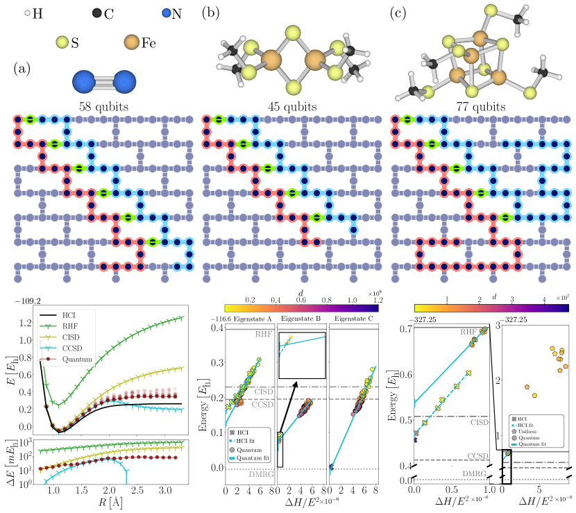
We perform two classes of experiments: the breaking of the triple bond of N2 (cc-pVDZ basis), in the top panel in Fig. 4 (a), and the ground states of [2Fe-2S] and [4Fe-4S] clusters (active spaces of the TZP-DKH basis), shown in the top panels in Fig. 4 (b) and (c). We study the ground-state properties of these molecular systems in the and subspace, where is the total component of the spin and .
Throughout our experiments we use the truncated LUCJ circuit , which is the result of considering the circuit and removing the last orbital rotation and Jastrow operations. We parameterize the LUCJ circuits converting the CCSD wavefunction in Jastrow form and imposing a locality approximation to the resulting tensors, i.e., zeroing out the components not corresponding to adjacent qubits [40]. For systems where the parameters obtained from CCSD have small amplitude, the and terms in the ansatz approximately cancel: in such situation, without , the resulting wavefunction is over-concentrated around the Hartree-Fock configuration [29].
The breaking of the N2 bond is a well-known test of the accuracy of electronic structure methods in the presence of static electronic correlation [43, 44]. Restricted CCSD theory, a dominant paradigm for the accurate description of weakly correlated systems in quantum chemistry, fails in the description of N2 dissociation due to static correlation effects: as correlations become stronger, RHF becomes unstable toward a symmetry-broken unrestricted Hartree-Fock (UHF) state. CCSD built from RHF predicts an artificial barrier to binding and over-correlates at dissociation, whereas CCSD built from a UHF reference dissociates correctly at the cost of spin contamination, a manifestation of Löwdin’s symmetry dilemma. We use a correlation-consistent cc-pVDZ basis set, to place emphasis on a theory’s ability to treat both dynamic and static correlation in an accurate and balanced manner. We map the N2 molecule onto a Heron processor as shown in the middle panel of Fig. 4 (a). We project and diagonalize a Hamiltonian using configurations. We consider batches of configurations and each point in the dissociation curve has measurement outcomes and 10 iterations of recovery. The experimental data is reported in the bottom panel of Fig. 4 (a), showing the potential energy surface of N2 compared to classical approximate methods. The data from our experiments are consistent with other classical methods except for CCSD, which fails in the description of the dissociation as seen for the smaller basis set considered in Fig. 4(b). Amongst the classical SCI methods, Heat-Bath Configuration Interaction (HCI) [35] obtains the best results for N2 and will be our reference classical method in all the other experiments. The difference between our method and HCI energies is everywhere within tens of . We further analyze the accuracy of our experiments as a function of , and the effect of orbital optimizations in the accuracy of the predictions [29]. This first test demonstrates that we are capable of addressing multi-reference ground states and builds confidence for the next set of experiments, which will focus on assessing the ability of the quantum-classical architecture to do precision many-body physics.
Iron–sulfur (FeS) clusters are molecular ensembles of sulfide-linked 1- to 8-iron centers in variable oxidation states. They are important cofactors in biological processes ranging from nitrogen fixation to photosynthesis and respiration [46]. Their electronic structure, with multiple low-lying states of differing electronic and magnetic character, is responsible for their rich chemistry. At the same time, they pose considerable challenges for experimental studies and numerical tools. For our experiments we consider the synthetic [Fe2S2(SCH3)4]-2 cluster [4], abbreviated [2Fe-2S] and used in numerical studies to mimic the oxidized dimers prominently found in ferredoxins [47].
The qubit mapping of the LUCJ circuit on the Heron processor for [2Fe-2S] is shown in the middle panel of Fig. 4 (b). We consider batches of configurations and measurement outcomes. For the [2Fe-2S] cluster, we perform an energy-variance analysis of the low-energy spectrum of the molecule. The energy-variance analysis is a tool routinely used in classical computational electronic structure to capture the convergence of the approximate eigenstate energy for different levels of accuracy of a computational method [48]. Here we use energy-variance analysis to assess the convergence as a function of , which is directly related to quantum and classical accuracy, runtimes, and costs. If one can statistically sample from a good approximation of an eigenstate, points at finite number of samples will be distributed linearly in the energy-variance plane [48]. This gives us a tool to detect eigenstates for both quantum and classical methods.
The bottom panel in Fig. 4(b) shows an energy-variance comparison of HCI and our estimator. The accuracy of both estimators is quantified by the number of electronic configurations that span the subspace for diagonalization. For , we warm start with the obtained from the method at , and only two recovery iterations are considered after. As we increase , three eigenstates appear, which we label A, B, and C. At lower values of , the data follows the expected linear relation for eigenstate A. Beyond a critical value of , both the energy and variance change abruptly, discovering another set of points following a linear relation, which correspond to a second eigenstate B, of lower energy. The resulting mean occupations of eigenstates A and B are substantially different [29], confirming that we have found two distinct eigenstates. The third cluster of points in the energy-variance plane (Eigenstate C) was found by warm starting the procedure, for all values of considered, with the obtained from the second cluster (Eigenstate B) at . We then extrapolate the quantum data following the linear energy-variance relations, finding agreement between the quantum extrapolated data and the best HCI calculation performed and the Density Matrix Renormalization Group (DMRG) calculaiton from Ref. [45], showcasing the ability of our methods to perform precision many-body physics.
The circuits considered for the N2 experiments and [2Fe-2S] reached sizes of approximately 1-1.5k two-qubit gates. We now test the quality of the signal in noisy circuits that test the limits of Heron devices, using up to 6400 nodes of Fugaku for the classical processing. We consider the synthetic [Fe4S4(SCH3)4]-2 cluster [4], abbreviated [4Fe-4S], a representative of nature’s cubanes, whose ground state deduction from experimental measurements was an early success of inorganic spectroscopy [49]. The LUCJ circuit employed for this molecular species contains approximately 3.5k two-qubit gates. The qubit mapping on the Heron processor for [4Fe-4S] is shown in the middle panel of Fig. 4 (c). As in the previous experiment, we consider batches of configurations and measurement outcomes. For , configuration recovery is warm started with the obtained from the method at , and only two iterations are then performed.
This last set of experiments sheds light on the quality of the quantum signal that is passed to the configuration recovery at these large circuit sizes. The bottom right panel in Fig. 4 (c) shows a comparison of the energy-variance analysis from measurement outcomes obtained from the Heron device and configurations sampled from the uniform distribution. We see that, even if the quantum solutions produced are worse than other classical methods, the energy and variance obtained from quantum data are significantly lower than those obtained from uniformly distributed configurations (i.e. pure noise), on subspaces of the same size. This confirms that there is a valuable signal at circuit sizes of approximately 3.5k two-qubit gates.
III Discussion
Current quantum computers in isolation can be used as tools to explore calculations beyond brute-force [50, 51] on problems that match the interactions of the quantum devices. The assistance of classical distributed computations enables addressing problems that go beyond this constraint, with workflows such as the one used here for chemistry.
We now discuss the implications of our results in the search for quantum advantage. Any computation is ranked against three parameters: runtime, energy or cost, and accuracy. While the first two are often easily measured, ranking by accuracy is not always straightforward. However, the class of computational methods that strictly produce upper bounds to the ground-state energy defines an unconditional accuracy metric, which can be used to assess quantum advantage. Within this class of methods, a lower energy is ranked as higher quality, with no extra information required. This, for example, allowed us to benchmark our results against classical selected configuration interaction and uniform configuration sampling on an experiment on 77 qubits, without access to exact solutions. Additionally, the approximate solutions found here can be stored in classical memory, which permits a classical prover to certify them, and allows their manipulation by further classical processing.
The estimator can be applied to simulation tasks other than quantum chemistry, if the target ground state energy can be captured by a sparse wavefunction. This motivates looking into useful quantum circuits with supports in the computational basis scaling polynomially with problem size. Although in principle other estimators, such as the standard ones used in variational quantum eigensolvers, have bounded variance for any wavefunction, the dire scaling of number of measurements to estimate energies makes them impractical for the molecules targeted in this work [3].
Reconstructing the exact ground state probability distribution on a quantum computer is not required to get accurate energy approximations, as long as one is sampling from the ground state support. It will be compelling to use these methods on future quantum devices with lower error rates and correspondingly reduced classical processing requirements.
To counter wavefunction broadening on current quantum hardware, we have used a self-consistent configuration recovery method, exploiting a problem-inspired clustering that leverages the average occupation numbers of the molecular orbitals. We foresee generalizations of our configuration recovery technique to problems other than quantum chemistry that are not informed by the physics of the problem. Conversely, for specific applications one could use even more information about the problem.
We have used a LUCJ class of quantum circuits that can reproduce a low-rank decomposition and sparsification of the quantum unitary CCSD (qUCCSD), which allowed us to keep circuit depths manageable [40]. Better quantum noise rates would allow to access deeper quantum circuits, improving their approximation of the qUCCSD theory and eventually surpassing qUCCSD itself if enough parameters are given. The inclusion of more density-density interactions, takes LUCJ further away from non-interacting fermionic computations, increasing the classical simulation overhead [52]. We have performed optimization-free experiments, exploiting the connection between LUCJ and classical coupled cluster theory, yet closing a quantum-classical optimization could further improve the quality of the solutions.
It is important to evaluate the methods presented here in the context of variational classical heuristics to highlight their different domains of applicability [53]. To improve on other classical CI methods, one would need to sample important configurations with a significant number of excitations over the HF state. Variational quantum Monte Carlo methods [54, 55], of paramount importance in many-body physics, are sensitive to the structures of the probability distributions they are modeling, not just to their supports. Methods based on tensor networks [56, 57] are successfully used to tackle strongly correlated problems in chemistry, granted the ability to converge their energies with bond dimensions. Convergence can be challenging in some cases [58, 59] because of its computational cost and its sensitivity to the nature and ordering of the basis-set orbitals. Characterizing the domain of applicability of different classical and quantum heuristics facilitates combining them in quantum-centric supercomputing environments, shifting the search for quantum advantage towards practical problems.
Author contributions
Design of the workflow and experiments: J. R.-M., M. M., W. K., K. S., M. T., A. M. Implementation of the workflow: J. R.-M., M. M., A. J.-A., S. M., S. S., T. S., I. S., R.-Y. S., K. J. S. Tuning and calibration of the Heron processor: H.H. Execution of the quantum part of the workflow on Heron: M. M., P. J., M. T. Execution of the classical part of the workflow on Fugaku: T. S., R.-Y. S., S. Y. Numerical benchmarks: J. R.-M., M.M., T. S., K. J. S. Analytical derivations: J. R.-M., M.M., W. K., K. S., M. T., A. M. All authors contributed to the manuscript writing and data analysis.
Acknowledgements.
We thank the IBM Quantum Service and Data team for help with the workflow execution. The authors acknowledge feedback and insightful conversations with Alberto Baiardi, Giuseppe Carleo, Garnet Kin-Lic Chan, Antonio Córcoles, Oliver Dial, Jay Gambetta, Artur Izmaylov, Yukio Kawashima, David Kremer, Isaac Lauer, Peter Love, Guglielmo Mazzola, Takahito Nakajima, Paul Nation, Hanhee Paik, Emily Pritchett, Max Rossmannek, Paul Schweigert, James E.T. Smith, Miles Stoudenmire, Andrew Wack, Christa Zoufal.References
- Feynman [1982] R. P. Feynman, Simulating physics with computers, Int. J. Theor. Phys 21, 467 (1982).
- Aspuru-Guzik et al. [2005] A. Aspuru-Guzik, A. D. Dutoi, P. J. Love, and M. Head-Gordon, Simulated quantum computation of molecular energies, Science 309, 1704 (2005).
- Wecker et al. [2015] D. Wecker, M. B. Hastings, and M. Troyer, Progress towards practical quantum variational algorithms, Phys. Rev. A 92, 042303 (2015).
- Sharma et al. [2014] S. Sharma, K. Sivalingam, F. Neese, and G. K.-L. Chan, Low-energy spectrum of iron-sulfur clusters directly from many-particle quantum mechanics, Nat. Chem 6, 927 (2014).
- Vogiatzis et al. [2017] K. D. Vogiatzis, D. Ma, J. Olsen, L. Gagliardi, and W. A. De Jong, Pushing configuration-interaction to the limit: towards massively parallel MCSCF calculations, J. Chem. Phys 147, 184111 (2017).
- Gao et al. [2024] H. Gao, S. Imamura, A. Kasagi, and E. Yoshida, Distributed implementation of full configuration interaction for one trillion determinants, J. Chem. Theory Comput (2024).
- LeBlanc et al. [2015] J. P. LeBlanc, A. E. Antipov, F. Becca, I. W. Bulik, G. K.-L. Chan, C.-M. Chung, Y. Deng, M. Ferrero, T. M. Henderson, C. A. Jiménez-Hoyos, et al., Solutions of the two-dimensional Hubbard model: benchmarks and results from a wide range of numerical algorithms, Phys. Rev. X 5, 041041 (2015).
- Motta et al. [2017] M. Motta, D. M. Ceperley, G. K.-L. Chan, J. A. Gomez, E. Gull, S. Guo, C. A. Jiménez-Hoyos, T. N. Lan, J. Li, F. Ma, et al., Towards the solution of the many-electron problem in real materials: equation of state of the hydrogen chain with state-of-the-art many-body methods, Phys. Rev. X 7, 031059 (2017).
- Cao et al. [2019] Y. Cao, J. Romero, J. P. Olson, M. Degroote, P. D. Johnson, M. Kieferová, I. D. Kivlichan, T. Menke, B. Peropadre, N. P. Sawaya, et al., Quantum chemistry in the age of quantum computing, Chem. Rev 119, 10856 (2019).
- McArdle et al. [2020] S. McArdle, S. Endo, A. Aspuru-Guzik, S. C. Benjamin, and X. Yuan, Quantum computational chemistry, Rev. Mod. Phys 92, 015003 (2020).
- Bauer et al. [2020] B. Bauer, S. Bravyi, M. Motta, and G. Kin-Lic Chan, Quantum algorithms for quantum chemistry and quantum materials science, Chem. Rev 120, 12685 (2020).
- Kandala et al. [2017] A. Kandala, A. Mezzacapo, K. Temme, M. Takita, M. Brink, J. M. Chow, and J. M. Gambetta, Hardware-efficient variational quantum eigensolver for small molecules and quantum magnets, Nature 549, 242 (2017).
- Google AI Quantum and Collaborators [2020] Google AI Quantum and Collaborators, Hartree-Fock on a superconducting qubit quantum computer, Science 369, 1084 (2020).
- Huggins et al. [2022] W. J. Huggins, B. A. O’Gorman, N. C. Rubin, D. R. Reichman, R. Babbush, and J. Lee, Unbiasing fermionic quantum Monte Carlo with a quantum computer, Nature 603, 416 (2022).
- Motta et al. [2023a] M. Motta, G. O. Jones, J. E. Rice, T. P. Gujarati, R. Sakuma, I. Liepuoniute, J. M. Garcia, and Y.-y. Ohnishi, Quantum chemistry simulation of ground- and excited-state properties of the sulfonium cation on a superconducting quantum processor, Chem. Sci 14, 2915 (2023a).
- Zhao et al. [2023] L. Zhao, J. Goings, K. Shin, W. Kyoung, J. I. Fuks, J.-K. Kevin Rhee, Y. M. Rhee, K. Wright, J. Nguyen, J. Kim, et al., Orbital-optimized pair-correlated electron simulations on trapped-ion quantum computers, npj Quantum Inf 9, 60 (2023).
- Google AI Quantum and Collaborators [2023] Google AI Quantum and Collaborators, Purification-based quantum error mitigation of pair-correlated electron simulations, Nat. Phys 19, 1787 (2023).
- Weaving et al. [2023] T. Weaving, A. Ralli, P. J. Love, S. Succi, and P. V. Coveney, Contextual subspace variational quantum eigensolver calculation of the dissociation curve of molecular nitrogen on a superconducting quantum computer (2023), arXiv:2312.04392 [quant-ph] .
- Verteletskyi et al. [2020] V. Verteletskyi, T.-C. Yen, and A. F. Izmaylov, Measurement optimization in the variational quantum eigensolver using a minimum clique cover, J. Chem. Phys 152, 124114 (2020).
- Huggins et al. [2021] W. J. Huggins, J. R. McClean, N. C. Rubin, Z. Jiang, N. Wiebe, K. B. Whaley, and R. Babbush, Efficient and noise resilient measurements for quantum chemistry on near-term quantum computers, npj Quantum Inf 7, 1 (2021).
- Dutt et al. [2023] A. Dutt, W. Kirby, R. Raymond, C. Hadfield, S. Sheldon, I. L. Chuang, and A. Mezzacapo, Practical benchmarking of randomized measurement methods for quantum chemistry Hamiltonians, arXiv:2312.07497 (2023).
- Anand et al. [2022] A. Anand, P. Schleich, S. Alperin-Lea, P. W. Jensen, S. Sim, M. Díaz-Tinoco, J. S. Kottmann, M. Degroote, A. F. Izmaylov, and A. Aspuru-Guzik, A quantum computing view on unitary coupled cluster theory, Chem. Soc. Rev 51, 1659 (2022).
- Hastings et al. [2015] M. B. Hastings, D. Wecker, B. Bauer, and M. Troyer, Improving quantum algorithms for quantum chemistry, Quant. Info. Comput 15, 1–21 (2015).
- Lee et al. [2021] J. Lee, D. W. Berry, C. Gidney, W. J. Huggins, J. R. McClean, N. Wiebe, and R. Babbush, Even more efficient quantum computations of chemistry through tensor hypercontraction, Phys. Rev. X Quantum 2, 030305 (2021).
- Alexeev et al. [2023] Y. Alexeev, M. Amsler, P. Baity, M. A. Barroca, S. Bassini, T. Battelle, D. Camps, D. Casanova, F. T. Chong, C. Chung, et al., Quantum-centric supercomputing for materials science: A perspective on challenges and future directions, arXiv preprint arXiv:2312.09733 (2023).
- Sun et al. [2018] Q. Sun, T. C. Berkelbach, N. S. Blunt, G. H. Booth, S. Guo, Z. Li, J. Liu, J. D. McClain, E. R. Sayfutyarova, S. Sharma, et al., PySCF: the python-based simulations of chemistry framework, WIREs Comput. Mol. Sci 8, e1340 (2018).
- Jordan and Wigner [1928] P. Jordan and E. Wigner, Über das paulische äquivalenzverbot, Zeit. Phys 47, 631 (1928).
- Ivanic and Ruedenberg [2001] J. Ivanic and K. Ruedenberg, Identification of deadwood in configuration spaces through general direct configuration interaction, Theor. Chem. Acc 106, 339 (2001).
- [29] See supplementary information.
- Kanno et al. [2023] K. Kanno, M. Kohda, R. Imai, S. Koh, K. Mitarai, W. Mizukami, and Y. O. Nakagawa, Quantum-selected configuration interaction: classical diagonalization of Hamiltonians in subspaces selected by quantum computers (2023), arXiv:2302.11320 [quant-ph] .
- Nakagawa et al. [2023] Y. O. Nakagawa, M. Kamoshita, W. Mizukami, S. Sudo, and Y. ya Ohnishi, ADAPT-QSCI: Adaptive construction of input state for quantum-selected configuration interaction (2023), arXiv:2311.01105 [quant-ph] .
- Evangelista [2014] F. A. Evangelista, Adaptive multiconfigurational wave functions, J. Chem. Phys 140, 124114 (2014).
- Schriber and Evangelista [2016] J. B. Schriber and F. A. Evangelista, Communication: An adaptive configuration interaction approach for strongly correlated electrons with tunable accuracy, J. Chem. Phys 144, 161106 (2016).
- Holmes et al. [2016a] A. A. Holmes, H. J. Changlani, and C. Umrigar, Efficient heat-bath sampling in Fock space, J. Chem. Theory Comput 12, 1561 (2016a).
- Holmes et al. [2016b] A. A. Holmes, N. M. Tubman, and C. Umrigar, Heat-bath configuration interaction: An efficient selected configuration interaction algorithm inspired by heat-bath sampling, J. Chem. Theory Comput 12, 3674 (2016b).
- Tubman et al. [2016] N. M. Tubman, J. Lee, T. Y. Takeshita, M. Head-Gordon, and K. B. Whaley, A deterministic alternative to the full configuration interaction quantum Monte Carlo method, J. Chem. Phys 145, 044112 (2016).
- Schriber and Evangelista [2017] J. B. Schriber and F. A. Evangelista, Adaptive configuration interaction for computing challenging electronic excited states with tunable accuracy, J. Chem. Theory Comput 13, 5354 (2017).
- Sharma et al. [2017] S. Sharma, A. A. Holmes, G. Jeanmairet, A. Alavi, and C. J. Umrigar, Semistochastic heat-bath configuration interaction method: Selected configuration interaction with semistochastic perturbation theory, J. Chem. Theory Comput 13, 1595 (2017).
- Evangelista et al. [2019] F. A. Evangelista, G. K.-L. Chan, and G. E. Scuseria, Exact parameterization of fermionic wave functions via unitary coupled cluster theory, J. Chem. Phys 151, 244112 (2019).
- Motta et al. [2023b] M. Motta, K. J. Sung, K. B. Whaley, M. Head-Gordon, and J. Shee, Bridging physical intuition and hardware efficiency for correlated electronic states: the local unitary cluster Jastrow ansatz for electronic structure, Chem. Sci 14, 11213 (2023b).
- Matsuzawa and Kurashige [2020] Y. Matsuzawa and Y. Kurashige, Jastrow-type decomposition in quantum chemistry for low-depth quantum circuits, J. Chem. Theory Comput 16, 944 (2020).
- The ffsim developers [2024] The ffsim developers, ffsim: Faster simulations of fermionic quantum circuits (2024).
- Fan and Piecuch [2006] P.-D. Fan and P. Piecuch, The usefulness of exponential wave function expansions employing one-and two-body cluster operators in electronic structure theory: The extended and generalized coupled-cluster methods, Adv. Quantum Chem 51, 1 (2006).
- Bulik et al. [2015] I. W. Bulik, T. M. Henderson, and G. E. Scuseria, Can single-reference coupled cluster theory describe static correlation?, J. Chem. Theory Comput 11, 3171 (2015).
- Li and Chan [2017a] Z. Li and G. K.-L. Chan, Spin-projected matrix product states: versatile tool for strongly correlated systems, J. Chem. Theory Comput 13, 2681 (2017a).
- Beinert et al. [1997] H. Beinert, R. H. Holm, and E. Munck, Iron-sulfur clusters: nature’s modular, multipurpose structures, Science 277, 653 (1997).
- Venkateswara Rao and Holm [2004] P. Venkateswara Rao and R. Holm, Synthetic analogues of the active sites of iron-sulfur proteins, Chem. Rev 104, 527 (2004).
- Kashima and Imada [2001] T. Kashima and M. Imada, Path-integral renormalization group method for numerical study on ground states of strongly correlated electronic systems, J. Phys. Soc. Jpn 70, 2287 (2001).
- Papaefthymiou et al. [1986] V. Papaefthymiou, M. M. Millar, and E. Muenck, Moessbauer and EPR studies of a synthetic analog for the iron-sulfur Fe4S4 core of oxidized and reduced high-potential iron proteins, Inorg. Chem 25, 3010 (1986).
- Kim et al. [2023] Y. Kim, A. Eddins, S. Anand, K. X. Wei, E. Van Den Berg, S. Rosenblatt, H. Nayfeh, Y. Wu, M. Zaletel, K. Temme, et al., Evidence for the utility of quantum computing before fault tolerance, Nature 618, 500 (2023).
- Shinjo et al. [2024] K. Shinjo, K. Seki, T. Shirakawa, R.-Y. Sun, and S. Yunoki, Unveiling clean two-dimensional discrete time quasicrystals on a digital quantum computer, arXiv preprint arXiv:2403.16718 (2024).
- Reardon-Smith et al. [2023] O. Reardon-Smith, M. Oszmaniec, and K. Korzekwa, Improved simulation of quantum circuits dominated by free fermionic operations, arXiv preprint arXiv:2307.12702 (2023).
- Lee et al. [2023] S. Lee, J. Lee, H. Zhai, Y. Tong, A. M. Dalzell, A. Kumar, P. Helms, J. Gray, Z.-H. Cui, W. Liu, et al., Evaluating the evidence for exponential quantum advantage in ground-state quantum chemistry, Nat. Commun 14, 1952 (2023).
- Becca and Sorella [2017] F. Becca and S. Sorella, Quantum Monte Carlo approaches for correlated systems (Cambridge University Press, 2017).
- Carleo and Troyer [2017] G. Carleo and M. Troyer, Solving the quantum many-body problem with artificial neural networks, Science 355, 602 (2017).
- White and Martin [1999] S. R. White and R. L. Martin, Ab initio quantum chemistry using the density matrix renormalization group, J. Chem. Phys 110, 4127 (1999).
- Chan and Sharma [2011] G. K.-L. Chan and S. Sharma, The density matrix renormalization group in quantum chemistry, Annu. Rev. Phys. Chem 62, 465 (2011).
- Hubig et al. [2018] C. Hubig, J. Haegeman, and U. Schollwöck, Error estimates for extrapolations with matrix-product states, Phys. Rev. B 97, 045125 (2018).
- Li et al. [2019] Z. Li, J. Li, N. S. Dattani, C. Umrigar, and G. K. Chan, The electronic complexity of the ground-state of the FeMo cofactor of nitrogenase as relevant to quantum simulations, J. Chem. Phys 150, 024302 (2019).
- Hehre et al. [1969] W. J. Hehre, R. F. Stewart, and J. A. Pople, Self-consistent molecular-orbital methods. I. use of Gaussian expansions of Slater-type atomic orbitals, J. Chem. Phys 51, 2657 (1969).
- Hehre et al. [1972] W. J. Hehre, R. Ditchfield, and J. A. Pople, Self-consistent molecular orbital methods. XII. Further extensions of Gaussian-type basis sets for use in molecular orbital studies of organic molecules, J. Chem. Phys 56, 2257 (1972).
- Dunning [1989] T. H. Dunning, Gaussian basis sets for use in correlated molecular calculations. I. The atoms boron through neon and hydrogen, J. Chem. Phys 90, 1007 (1989).
- Sun et al. [2020] Q. Sun, X. Zhang, S. Banerjee, P. Bao, M. Barbry, N. S. Blunt, N. A. Bogdanov, G. H. Booth, J. Chen, Z.-H. Cui, et al., Recent developments in the PySCF program package, J. Chem. Phys 153, 024109 (2020).
- Becke [1988] A. D. Becke, Density-functional exchange-energy approximation with correct asymptotic behavior, Phys. Rev. A 38, 3098 (1988).
- Perdew [1986] J. P. Perdew, Density-functional approximation for the correlation energy of the inhomogeneous electron gas, Phys. Rev. B 33, 8822 (1986).
- Jorge et al. [2009] F. Jorge, A. Canal Neto, G. Camiletti, and S. Machado, Contracted Gaussian basis sets for Douglas-Kroll-Hess calculations: estimating scalar relativistic effects of some atomic and molecular properties, J. Chem. Phys 130 (2009).
- Liu [2010] W. Liu, Ideas of relativistic quantum chemistry, Mol. Phys 108, 1679 (2010).
- Li et al. [2012] Z. Li, Y. Xiao, and W. Liu, On the spin separation of algebraic two-component relativistic Hamiltonians, J. Chem. Phys 137, 154114 (2012).
- Tang et al. [2021] H. L. Tang, V. Shkolnikov, G. S. Barron, H. R. Grimsley, N. J. Mayhall, E. Barnes, and S. E. Economou, Qubit-ADAPT-VQE: an adaptive algorithm for constructing hardware-efficient ansaatzes on a quantum processor, PRX Quantum 2, 020310 (2021).
- Powell [1994] M. J. D. Powell, A direct search optimization method that models the objective and constraint functions by linear interpolation, in Advances in Optimization and Numerical Analysis, edited by S. Gomez and J.-P. Hennart (Springer Netherlands, Dordrecht, 1994) pp. 51–67.
- Roos et al. [1980] B. O. Roos, P. R. Taylor, and P. E. Sigbahn, A complete active space SCF method (CASSCF) using a density matrix formulated super-CI approach, Chem. Phys 48, 157 (1980).
- Head-Gordon and Pople [1988] M. Head-Gordon and J. A. Pople, Optimization of wave function and geometry in the finite basis Hartree-Fock method, J. Phys. Chem 92, 3063 (1988).
- Werner and Knowles [1985] H.-J. Werner and P. J. Knowles, A second order multiconfiguration SCF procedure with optimum convergence, J. Chem. Phys 82, 5053 (1985).
- Olsen [2011] J. Olsen, The CASSCF method: A perspective and commentary, Int. J. Quantum Chem 111, 3267 (2011).
- Zgid and Nooijen [2008] D. Zgid and M. Nooijen, The density matrix renormalization group self-consistent field method: orbital optimization with the density matrix renormalization group method in the active space, J. Chem. Phys 128, 144116 (2008).
- Wu et al. [2022] A.-K. Wu, M. T. Fishman, J. Pixley, and E. Stoudenmire, Disentangling interacting systems with fermionic gaussian circuits: application to the single impurity Anderson model, arXiv:2212.09798 (2022).
- Wouters and Van Neck [2014] S. Wouters and D. Van Neck, The density matrix renormalization group for ab initio quantum chemistry, Eur. Phys. J. D 68, 272 (2014).
- Moreno et al. [2023] J. R. Moreno, J. Cohn, D. Sels, and M. Motta, Enhancing the expressivity of variational neural, and hardware-efficient quantum states through orbital rotations (2023), arXiv:2302.11588 [quant-ph] .
- Sokolov et al. [2020] I. O. Sokolov, P. K. Barkoutsos, P. J. Ollitrault, D. Greenberg, J. Rice, M. Pistoia, and I. Tavernelli, Quantum orbital-optimized unitary coupled cluster methods in the strongly correlated regime: can quantum algorithms outperform their classical equivalents?, J. Chem. Phys 152, 124107 (2020).
- Mizukami et al. [2020] W. Mizukami, K. Mitarai, Y. O. Nakagawa, T. Yamamoto, T. Yan, and Y.-y. Ohnishi, Orbital optimized unitary coupled cluster theory for quantum computer, Phys. Rev. Research 2, 033421 (2020).
- Bierman et al. [2023] J. Bierman, Y. Li, and J. Lu, Improving the accuracy of variational quantum eigensolvers with fewer qubits using orbital optimization, J. Chem. Theory Comput 19, 790 (2023).
- Smith et al. [2017] J. E. Smith, B. Mussard, A. A. Holmes, and S. Sharma, Cheap and near exact casscf with large active spaces, Journal of chemical theory and computation 13, 5468 (2017).
- Thouless [1960] D. Thouless, Stability conditions and nuclear rotations in the Hartree-Fock theory, Nuc. Phys 21, 225 (1960).
- Bradbury et al. [2018] J. Bradbury, R. Frostig, P. Hawkins, M. J. Johnson, C. Leary, D. Maclaurin, G. Necula, A. Paszke, J. VanderPlas, S. Wanderman-Milne, and Q. Zhang, JAX: composable transformations of Python+NumPy programs (2018).
- Chowdhury et al. [2022] D. Chowdhury, A. Georges, O. Parcollet, and S. Sachdev, Sachdev-Ye-Kitaev models and beyond: window into non-Fermi liquids, Rev. Mod. Phys. 94, 035004 (2022).
- Friedman and Levine [1997] B. Friedman and G. Levine, Configuration-interaction approach to the two-dimensional Hubbard model near half-filling, Phys. Rev. B 55, 9558 (1997).
- Louis et al. [1999] E. Louis, F. Guinea, M. P. López Sancho, and J. A. Vergés, Configuration-interaction approach to hole pairing in the two-dimensional Hubbard model, Phys. Rev. B 59, 14005 (1999).
- Schwarz et al. [2015] L. R. Schwarz, G. H. Booth, and A. Alavi, Insights into the structure of many-electron wave functions of mott-insulating antiferromagnets: The three-band Hubbard model in full configuration interaction quantum Monte Carlo, Phys. Rev. B 91, 045139 (2015).
- Dobrautz et al. [2019] W. Dobrautz, H. Luo, and A. Alavi, Compact numerical solutions to the two-dimensional repulsive Hubbard model obtained via nonunitary similarity transformations, Phys. Rev. B 99, 075119 (2019).
- Rozenberg et al. [1994] M. J. Rozenberg, G. Kotliar, and X. Y. Zhang, Mott-Hubbard transition in infinite dimensions. II, Phys. Rev. B 49, 10181 (1994).
- Georges et al. [1996] A. Georges, G. Kotliar, W. Krauth, and M. J. Rozenberg, Dynamical mean-field theory of strongly correlated fermion systems and the limit of infinite dimensions, Rev. Mod. Phys. 68, 13 (1996).
- Lee et al. [2017] S.-S. B. Lee, J. von Delft, and A. Weichselbaum, Doublon-holon origin of the subpeaks at the Hubbard band edges, Phys. Rev. Lett. 119, 236402 (2017).
- Gauvin-Ndiaye et al. [2023] C. Gauvin-Ndiaye, J. Tindall, J. R. Moreno, and A. Georges, Mott transition and volume law entanglement with neural quantum states (2023), arXiv:2311.05749 [cond-mat.str-el] .
- Kwon et al. [1998] Y. Kwon, D. M. Ceperley, and R. M. Martin, Effects of backflow correlation in the three-dimensional electron gas: Quantum Monte Carlo study, Phys. Rev. B 58, 6800 (1998).
- Imada and Kashima [2000] M. Imada and T. Kashima, Path-integral renormalization group method for numerical study of strongly correlated electron systems, J. Phys. Soc. Jpn 69, 2723 (2000).
- Nomura et al. [2017] Y. Nomura, A. S. Darmawan, Y. Yamaji, and M. Imada, Restricted Boltzmann machine learning for solving strongly correlated quantum systems, Phys. Rev. B 96, 205152 (2017).
- Sorella [2001] S. Sorella, Generalized Lanczos algorithm for variational quantum Monte Carlo, Phys. Rev. B 64, 024512 (2001).
- Mizusaki and Imada [2002] T. Mizusaki and M. Imada, Extrapolation method for shell model calculations, Phys. Rev. C 65, 064319 (2002).
- Motta et al. [2021] M. Motta, E. Ye, J. R. McClean, Z. Li, A. J. Minnich, R. Babbush, and G. K.-L. Chan, Low rank representations for quantum simulation of electronic structure, npj Quantum Inf 7, 1 (2021).
- Reck et al. [1994] M. Reck, A. Zeilinger, H. J. Bernstein, and P. Bertani, Experimental realization of any discrete unitary operator, Phys. Rev. Lett 73, 58 (1994).
- Clements et al. [2016] W. R. Clements, P. C. Humphreys, B. J. Metcalf, W. S. Kolthammer, and I. A. Walmsley, Optimal design for universal multiport interferometers, Optica 3, 1460 (2016).
- Jiang et al. [2018] Z. Jiang, K. J. Sung, K. Kechedzhi, V. N. Smelyanskiy, and S. Boixo, Quantum algorithms to simulate many-body physics of correlated fermions, Phys. Rev. Appl 9, 044036 (2018).
- Nation et al. [2021] P. D. Nation, H. Kang, N. Sundaresan, and J. M. Gambetta, Scalable mitigation of measurement errors on quantum computers, Phys. Rev. X Quantum 2, 040326 (2021).
- Viola and Lloyd [1998] L. Viola and S. Lloyd, Dynamical suppression of decoherence in two-state quantum systems, Phys. Rev. A 58, 2733 (1998).
- Kofman and Kurizki [2001] A. Kofman and G. Kurizki, Universal dynamical control of quantum mechanical decay: modulation of the coupling to the continuum, Phys. Rev. Lett 87, 270405 (2001).
- Biercuk et al. [2009] M. J. Biercuk, H. Uys, A. P. VanDevender, N. Shiga, W. M. Itano, and J. J. Bollinger, Optimized dynamical decoupling in a model quantum memory, Nature 458, 996 (2009).
- Niu and Todri-Sanial [2022] S. Niu and A. Todri-Sanial, Effects of dynamical decoupling and pulse-level optimizations on IBM quantum computers, IEEE Trans. Quantum Eng 3, 1 (2022).
- Qiskit contributors [2023] Qiskit contributors, Qiskit: An open-source framework for quantum computing (2023).
- Li and Chan [2017b] Z. Li and G. K.-L. Chan, Repository: Active space model for iron sulfur clusters (2017b).
- Note [1] When considering samples from the uniform distribution over electronic configurations on the correct particle sector, the configuration recovery method cannot be applied since it only recovers configurations with the wrong particle number. Therefore, this scenario is equivalent to running QSCI (without configuration recovery) on those samples.
Supplementary Information: Chemistry Beyond Exact Solutions on a Quantum-Centric Supercomputer
I Conventions and notation
I.1 Hamiltonian
Our starting point is the Born-Oppenheimer Hamiltonian, written in second quantization using a basis of orthonormal orbitals ,
| (S1) |
Indices label spatial orbitals in the basis set, are spin indices, and the fermionic operator creates/destroys an electron in orbital with spin . We define the number operator which describes the number of electrons with spin on orbital . For non-relativistic all-electron calculations, the quantities
| (S2) |
describe the internuclear electrostatic interaction energy and the one-electron and two-electron parts of the Hamiltonian respectively (atomic units are used throughout, i.e. lengths and energies are measured in Bohr and Hartree units and respectively where and are the electron charge and mass). The symbols , , and denote the total number of nuclei and their positions and atomic numbers respectively.
For relativistic and/or active-space calculations, the indices label active-space orbitals, and the quantities , , and are modified to account for relativistic effects and/or the potential generated by the inactive-electron density.
In this work, we use orbitals from a restricted closed-shell Hartree-Fock calculation (also called molecular orbitals and denoted MOs) as the basis functions . Furthermore, we denote the number of spin- electrons in the exact ground state. Furthermore , the toal number of electrons in the exact ground state.
I.2 Molecular species and active spaces
| molecule | basis | ||
|---|---|---|---|
| N2 | 6-31G | (10e,16o) | |
| N2 | cc-pVDZ | (10e,26o) | |
| [2Fe-2S] | TZP-DKH | (30e,20o) | |
| [4Fe-4S] | TZP-DKH | (54e,36o) |
The molecules simulated in this work are listed in Table 1. For N2 , we studied all non-core electrons and orbitals on quantum hardware. We computed the potential energy curve using (i) restricted Hartree-Fock (RHF) at 6-31G, and cc-pVDZ level [60, 61, 62] using PySCF [26, 63] and enforcing symmetry and, after projecting the non-relativistic Born-Oppenheimer Hamiltonian in the space spanned by all non-core RHF orbitals with standard functionalities, with (ii) restricted and symmetry-preserving Moller-Plesset second-order perturbation theory (MP2), coupled cluster with singles and doubles (CCSD), complete active-space configuration interaction (CASCI), for 6-31G and selected configuration interaction, in its heat-bath flavor (HCI), for cc-pVDZ.
For [2Fe-2S] and [4Fe-4S] , we employed active spaces [4, 45], spanned by Fe[3d] and S[3p] orbitals, derived from a localized Density Functional Theory calculation with BP86 functional [64, 65], TZP-DKH basis [66], and sf-X2C (spin-free exact two-component) Hamiltonian [67, 68] to include scalar relativistic effects. We computed approximations to the ground-state energy with restricted RHF, MP2, CCSD, and HCI. The RHF, MP2, CCSD, CISD, CASCI and HCI calculations were carried out with the PySCF library [26].
I.3 Electron configurations and qubit mapping
In this work, we represent many-electron states using qubit states with the Jordan-Wigner transformation, that maps an electronic configuration, i.e. a Slater determinant of the form
| (S3) |
where is the vacuum state (i.e., the state with zero electrons) and , onto an element of the computational basis,
| (S4) |
labeled by a bitstring . The first half of the bitstring is denoted by and the second half of the bitstring is denoted by . The JW mapping employs qubits and allows computing the number of spin- electrons for a given configuration as . The total number of electrons, , is the Hamming weight of . At the single-configuration level, any in the right particle sector must satisfy: . An important example is the restricted Hatree-Fock (RHF) bitstring
| (S5) |
which by construction has .
The Fock space is the vector space containing all possible electronic configurations for orbitals with all possible filling factors for each spin sector. The terms determinant and electronic configuration are used interchangeably in the manuscript.
II Methods
II.1 HPC quantum estimator
This section provides a detailed description of the HPC quantum estimator. We describe the subspace projection and diagonalization, the self-consistent configuration recovery scheme, a lower bound to the likelihood of recovering different families of electronic configurations, and different techniques to optimize circuit parameters to minimize the estimator energy.
We first introduce some notations. We use and to denote a set of configurations sampled from probability distributions and , where is a density operator corresponding to a noisy version of . We denote the subset of configurations with the right particle number. The set of configurations recovered by the configuration recovery procedure is denoted by and the set of configurations output by self-consistent configuration recovery, and with a set of approximately configurations sampled from . The wavefunction in obtained by projection and diagonalization of in the subspace spanned by the configurations in .
II.1.1 Eigenstate solver
Given a set of electronic configurations, the many-electron Hamiltonian is projected and diagonalized in the subspace spanned by the single-particle states defined by the electronic configurations, as proposed recently in [30]. We begin by considering a set of configurations , all with the right-particle number for each spin sector. Sub-indices between parenthesis label configurations in a set and not configuration components. We use the generic label for a set of configurations with the right particle number. In practice, the configuration recovery procedure will execute the eigenstate solver on the sets and .
Conservation of spin.–
In this study, we ensured that our calculations produced wavefunctions that are eigenfunctions of Hamiltonian symmetries and in particular singlet states, i.e., eigenfunctions of total spin with eigenvalue 0, . Conservation of symmetries is notoriously important because molecular eigenstates are joint eigenfunctions of and its symmetries, including , , molecular point-group symmetries (if any), and . Conservation of and (and molecular point-group symmetries that are isomorphic to ) can be achieved in a relatively easy way, since the eigenfunctions of these operators are Slater determinants (SD) , e.g.
| (S6) |
Therefore, in this work, we ensure that the configurations used to span the SCI subspace all have the desired eigenvalue of and as part of the configuration recovery procedure in the presence of noise. Conservation of is more difficult to achieve in CI methods since the eigenfunctions of are not SDs. The proper way of ensuring conservation of is expanding on a set of configuration state functions (CSFs), i.e. spin-symmetry-adapted linear combinations of SDs. The use of CSFs was common in early CI codes since, in addition to the obvious benefits of reducing the memory footprint of the CI vector, automatic conservation of total spin enhanced the stability of the CI iterations. Modern CI codes tend to employ SDs as opposed to CSFs, because the formation of the vector (the most memory- and rate-limiting step of CI algorithms) is considerably more efficient and easily parallelized in SD-based algorithms, and in part because system memory and disk are more plentiful than in previous machines. However, in SD-based CI codes, the conservation of total spin is no longer guaranteed. In the case of our HPC quantum estimator, sampling from a quantum computer may return sets of SDs that do not allow constructing eigenfunctions of total spin. For example, in a (2e,2o) system, one may sample the configuration (having a single spin-down excitation over the RHF state ) which is a linear combination of the open-shell singlet and triplet states, respectively . If the configuration is not sampled, one can construct neither eigenfunction of total spin, leading to spin contamination or redundancy (i.e. the configuration is involved in a CI calculation, but has coefficient in the CI vector). In this work, to facilitate conservation of total spin, we relied on the following procedure: instead of collecting directly i.i.d. samples from to make the batch , we collect samples and identify all unique configurations (u for unique) of length obtained from and for , forming the set . The size of the set is upper bounded by . From we obtain the batch set as:
| (S7) |
The size of the set above is upper bounded by . This procedure facilitates total spin conservation (for example, from the configuration one can build the set , which contains two closed-shell configurations and allows constructing an open-shell singlet state) but does not enforce it. Therefore, in combination with the sampling strategy mentioned above, we achieve the conservation of total spin by a soft constraint in the eigenstate solver, i.e. by adding a penalty term to mitigate spin contamination,
| (S8) |
where can be understood as a Lagrange multiplier that penalizes contributions from . In this work, we employed a soft constraint with .
Projection and diagonalization.–
For each subsampled set , the Hamiltonian is projected into the corresponding subspace spanned by the configurations in :
| (S9) |
We then diagonalize this projected Hamiltonian (solving ), and its ground state forms an approximation to the ground state of . The approximate ground state is defined by its amplitudes in the subspace:
| (S10) |
The estimate of the ground-state energy is given by:
| (S11) |
II.1.2 Self-consistent configuration recovery
After a quantum state , corresponding to a noiseless state , is prepared in our pre-fault-tolerant quantum processor, we measure it in the computational basis, obtaining the set of measurements
| (S12) |
The class of noiseless states considered in this work are eigenstates to the total particle number operator and the total number operator for each spin species:
| (S13) |
From the measurements on the quantum processors, we observe that there are a number of configurations in whose and do not match the and of the ground state. In Table 2 we report typical values of the fraction of sampled configurations with the wrong particle number. Since the circuits we use to produce are particle-number preserving, we are certain that configurations with wrong particle numbers have been corrupted by noise. It is this subset of configurations that the configuration recovery scheme is applied to. The configurations in whose and are not subject to the configuration recovery subroutine.
We then probabilistically flip bits and restore the correct particle number using information obtained from observables of the system. We use the spin-orbital occupancy averaged over all collected batches of subsamples , whose components are given by:
| (S14) |
where is defined in Eq. (S10). Consider a configuration with spin-up electrons, where . From the set of occupied spin-orbitals in the first half of , bits are sampled to be flipped. If instead , the bits to be flipped are instead sampled from the unoccupied spin-orbitals. The same procedure applies to the spin-down orbitals.
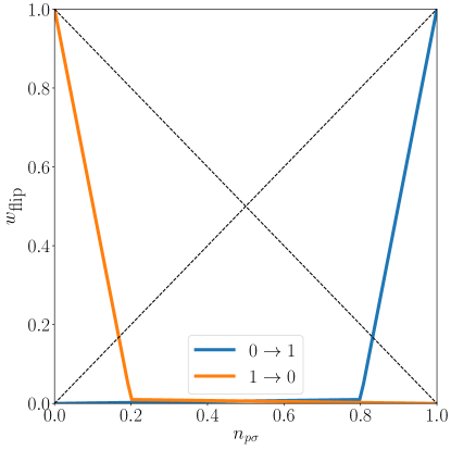
The probability of flipping bit depends on the distance between the value of the bit and the reference orbital occupancy . The simplest approach would be to define the distribution proportional to . However, this introduces an undesirable effect: if for some spin-orbital , , then as well, i.e., we assign roughly probability weight to flip the bit, regardless of its initial value. On the other hand, the initial value will in general retain some correlation with the other values in the bitstring, even in the presence of noise. Hence a better approach is to de-weight the probability of flipping when is small by using a modified rectified linear unit (ReLU) function , defined as
| (S15) |
The parameter defines the location of the “corner” of the ReLU function, while the parameter defines the value of the ReLU function at the corner. becomes a true ReLU function when , and for values of the ReLU is modified so that it is not identically zero except at : a plot is shown in Fig. S1. In the specific cases in this work, we chose the values and (the filling factor) in all experiments.
We do not assume that we know a priori, and instead we compute it and improve it self-consistently, following the procedure:
-
1.
Setup phase:
-
2.
Self-consistent iterations (repeat until stopping criterion is met):
-
(a)
is used to correct the configurations with the wrong particle number in (we give this subset the label ). The resulting set of recovered configurations is labelled .
-
(b)
From , batches of samples are obtained as described in Sec. II.1.1.
- (c)
-
(d)
From the approximate eigenstates construct refined guess for , according to Eq. (S14).
-
(e)
If the stopping criterion is not met, go back to step 2.(a).
-
(a)
We direct the reader to Fig. 2 in the main text for a numerical emulation of the effect of the configuration recovery on the accuracy of the HPC quantum estimator in the presence of noise.
An analytical lower bound to the probability of recovering families of configurations.–
Without loss of generality, we reorder the orbital labels such that . Note that in the previous expression we have combined the spin-orbital multi index into a single index running from . In the following we assume that there exists a good reference configuration , obtained by assigning value 1 to the bits of which have the largest magnitude, and zero otherwise. The average deviation of from is quantified by : . represents the average distance between each bit in and the corresponding entry in . The bits for which are referred to as the 1-sector of , while the bits for which are referred to as the 0-sector of . For this analysis we take the probability of flipping a bit in proportional to , which on average takes the value:
-
•
; if is in the 1-sector of and .
-
•
; if is in the 1-sector of and .
-
•
; if is in the 0-sector of and .
-
•
; if is in the 0-sector of and .
We use these average values for our analytical derivations.
We analyze the probability of recovering configurations using the configuration recovery scheme described above, as a function of their Hamming distance from . For this analysis, we consider a simple global depolarizing noise model, whose effect on the probability of sampled configurations is described by:
| (S16) |
where is a parameter that quantifies the amount of quantum signal. While we use for simplicity a global depolarizing noise model, we foresee similar derivations could be done for more realistic noise models.
The configurations that can be sampled from such a probability distribution fall into three categories: configurations with the right particle number that are in the support of the ideal distribution , configurations with the right particle number that are not the support of , and configurations with the wrong particle number. Configuration recovery does not apply to the first two categories. The third category, configurations with incorrect particle numbers, are guaranteed to have come from the noisy part of . We now derive a lower bound on the probability of drawing a configuration with wrong number of particles from and then converting it (via the configuration recovery scheme) to a particular configuration with the right particle number, whose Hamming distance to is .
Since is Hamming distance from , it contains s in the -sector and s in the -sector. There are two cases for initial configurations with wrong number of particles: those that have too many 1s or too many 0s.
-
1.
Too many 1s. In this case only bits with the value 1 will be flipped by the configuration recovery. Consider the set of initial noisy configurations with Hamming weight . Here, is the number of 1s in the 0-sector of in the initial configuration that need to be flipped to reach , while is the number of 1s in the 1-sector that need to be flipped to reach . All possible combinations of and are considered in this analysis. Starting from the initial noisy configuration, the probability of flipping one of the s that need to be flipped to reach (which we will call a “successful” bit-flip) is given by
(S17) the denominator reflects the total number of s weighted by their probabilities of being flipped. After flipping the first 1 in the 0-sector, the probability of another successful bit-flip in the the same sector is similarly
(S18) Thus, the probability of flipping all of the incorrect s in the 0-sector is
(S19) The same argument can be applied to the bit-flips performed in the 1-sector. The probability of a successful first bit-flip in the 1-sector is given by:
(S20) by essentially the same argument as above. The probability of a successful second flip is
(S21) One can apply the same iterative argument in this case. Hence, the overall probability of obtaining the target bitstring via configuration recovery is
(S22) -
2.
For the set of configurations with Hamming weight that came from and instances of bit-flip errors in the one- and zero-sectors of the state (respectively), a symmetric argument applies. We omit the derivation for this case.
The above gives the probabilities of recovering configurations with excess 1s or 0s back to a particular bitstring of Hamming distance from . We now integrate this probability over different values of and to obtain the probability of recovering a particular bitstring of Hamming distance to , from a sample drawn from the uniform distribution. We obtain the lower bound
| (S23) |
The two terms correspond to the two cases above, with the combinatorial fractions in each giving the probabilities of obtaining a configuration equivalent to the particular bitstring plus random bit-flips in the 0-sector of and random bit-flips in the 1-sector (first term), or random bit-flips in the one-sector of the HF state and random bit-flips in the zero-sector (second term).
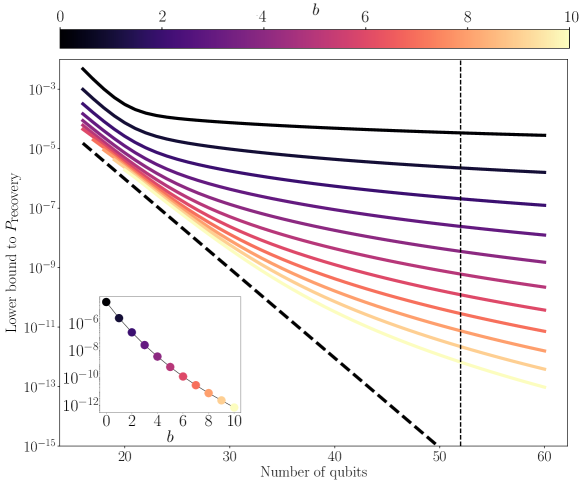
Fig. S2 shows the lower bound in Eq. (S23) to the recovery probability, for and , as a function of the number of qubits . We observe that the lower bound decays as an exponential of the number of qubits and that the recovery of configurations with small values of is more likely than the recovery of configurations defined by large values. We remark that the configuration recovery probability for configurations close to is substantially larger than the probability of obtaining the same samples by sampling from the uniform distribution, which would be the limit of no quantum signal. We argue that this feature helps in improving molecular energies over using simple post-selection over correct particle sector.
II.1.3 Optimization of the circuit parameters
The optimization of circuit parameters to produce better distributions in the space of electronic configurations is an avenue of improvement of the HPC quantum estimator framework. We develop a formalism for parameter optimization using the subspace energy as the cost function, in contrast to previous experiments that rely on standard VQE optimization frameworks [30, 31]. The HPC quantum estimator is constructed by running a diagonalization procedure in subspaces defined by different batches of sampled configurations, as described in Sec. II.1.1. The number of subspaces considered can go from to , where . Recall that is the dimensionality of the subspace of the Fock space spanned by configurations with the correct particle number and is the dimension of the SCI subspace. Note that is double-combinatorial in the number of spin-orbitals and electrons. Therefore, computing the HPC quantum estimator (with or without configuration recovery) for all possible sets of configurations is not efficient. Instead, we propose the use of a Monte Carlo estimator over batches of configurations to optimize the energy of the HPC quantum estimator averaged over different sets of configurations.
Recall that each configuration is sampled with probability , in the noiseless case. The following discussion applies to the noisy distribution . The method presented in this section can be applied also in conjunction with the configuration recovery technique. Since each configuration is i.i.d. sampled, the joint distribution that describes the probability of sampling the configurations in a batch with configurations is given by
| (S24) |
We consider the situation where the quantum circuit that prepares is characterized by a set of variational parameters . The explicit dependence on variational parameters is denoted by . A cost function is formulated for the circuit optimization:
| (S25) |
where is defined in Sec. II.1.1, Eq. (S11) as the SCI ground-state energy for the configurations in . An estimator to the double combinatorially-large summation in can be obtained by the Monte-Carlo unbiased estimator:
| (S26) |
with and where the are obtained from sampled according to . The gradient of the cost function with respect to the variational parameters is given by:
| (S27) |
Multiplying each term in the sum from the product rule by we obtain:
| (S28) |
whose Monte-Carlo estimator is given by:
| (S29) |
with and where again the are obtained from sampled according to . The evaluation of may be achieved by:
| (S30) |
We remark that the limit where is equivalent to the stochastic gradient-descent optimization technique.
For most classes of variational circuits, the gradient of the circuits may be implemented by parameter-shift rules or similar techniques. The reader may have noticed that the estimator for the gradient in the cost function of Eq. (S29) is biased if the support of does not coincide with the support of , as a direct consequence of writing for configurations outside the support of , where that expression is ill-defined.
Another practical issue with the gradient-based optimization of is the requirement to evaluate and , which rely in the Hadamard test for their evaluation. The implementation of the Hadamard test requires controlled versions of the circuits that realize the variational states. The implementation of such controlled unitaries requires circuit depths beyond the reach of current quantum devices.
An alternative approach is to optimize by explicit-gradient-free methods like COBYLA [70] or simulated annealing. Gradient-free optimization of the circuit parameters is used in the numerical study of Sec. III.1.4.
The optimization of the circuit parameters on quantum experiments to minimize the estimator energy will be the subject of future studies, which should consider the effect of noise in different gradient-free optimizers. Furthermore, the goal of this work is not to show that the optimization of the circuit parameters can improve the accuracy of the estimator, but to show that the quantum centric supercomputing estimator allows to tackle electronic structure problems described by an unprecedented number of qubits. Moreover, we show that the estimator run on circuits with fixed parameters already achieves good levels of accuracy.
II.1.4 Orbital optimization
We advise the reader to first visit Sec. II.1.3, since the cost function that is optimized is similar in this scenario. Orbital or single-particle basis rotations are a common approach to improve the accuracy of variational calculations of electronic structure systems. Orbital optimizations can be applied in conjunction with a wide variety of electronic structure methods, including complete active space diagonalizations [71, 72, 73, 74], the density matrix renormalization group [75, 76, 77], variational Monte Carlo [78] techniques, and quantum computing variational approaches [79, 80, 81]. Moreover, orbital optimizations are common practice on SCI-based approaches as well [82]. More generally, orbital optimizations make variational approaches invariant under orbital rotations. For notation clarity we replace in this section the notation of the two-body integral by the abbreviation .
The implementation of the orbital optimizations in conjunction with the HPC quantum estimator (with or without configuration recovery) follows the procedure presented in Ref. [78]. Orbital rotations consist of the application of the similarity transformation:
| (S31) |
where
| (S32) |
In this work, we choose the matrix that parametrizes the rotation to be real: . To enforce unitarity in we require that . According to Thouless’s Theorem [83], the action of the similarity transformation defined by transforms the creation operators according to:
| (S33) |
where . The Hamiltonian in the rotated basis can therefore be written in terms of the reference creation and annihilation operators:
| (S34) |
where the one- and two-body integrals have been transformed according to the tensor transformations:
| (S35) |
using Einstein’s summation convention.
A variational procedure is used to search for the single-particle basis that yields the optimal description of the ground state, given the collection of all possible bare variational trial states . The variational procedure is similar to the method presented in Sec. II.1.3. In this setting, is the SCI ansatz given as the linear combination of the determinants in (see Eq. (S10)). The set of variational parameters is composed of the circuit parameters defining together with the wavefunction amplitudes in the subspace defined by the SCI configurations. Each variational state is dressed by the same single-particle orbital rotation
| (S36) |
The loss function to be optimized in the variational setting is defined by the average, over batches of configurations, of the Rayleigh quotient:
| (S37) |
Gradient descent and its variants can be used to minimize both and in , while the optimization of is carried out by the diagonalization procedure (see Sec. II.1.1). Note that the sum in the average contains double-combinatorially many terms. Consequently, a Monte-Carlo based estimator is used to obtained an unbiased estimate (see Sec. II.1.3). Gradients with respect to have the same expression as in Eq. (S28) replacing by . Gradients with respect to the orbital rotations can be computed by the contraction of the bare one- and two-body reduced density matrices (1- and 2-RDMs) with the gradients of the one- and -two body integrals with respect to in Eq. (S37):
| (S38) |
In the previous expression the gradients of the integrals in the rotated basis are given by
| (S39) |
and the bare 1-RDMs and 2-RDMs are defined as
| (S40) |
The gradients of the integrals with respect to the rotation parameters are computed using the automatic differentiation (AD) tools of the software package Jax [84]. Since the evaluation of the gradients with respect to requires the evaluation of an intractable sum, we use an unbiased Monte-Carlo estimator for its evaluation:
| (S41) |
with and where the batches of configurations labelled by are sampled according to (see Eq. (S24)).
For a full orbital optimization calculation, all sets of variational parameters , , and should be updated. Since and sets rely on gradients for their optimization, they can be updated simultaneously. However, the wavefunction amplitudes are not updated by gradients. In this case, the optimization strategy consists of the alternation of a number of gradient-descent steps optimizing and followed by the eigenstate solver that now uses samples from an updated distribution according to the change in with a rotated Hamiltonian according to . This alternation is repeated for a number of iterations . In this work, we do not consider the optimization of circuit parameters and therefore the effect of the orbital optimization is not maximized, since the quantum circuit is not allowed to respond to the change in the Hamiltonian.
See Sec. IV.3 to see the effect of orbital optimizations in the accuracy of the HPC quantum estimator (with configuration recovery). The section shows results run on measurement outcomes obtained from the Heron device, to study the dissociation of N2 at cc-pVDZ level of theory.
II.2 Wavefunction concentration and accuracy
II.2.1 Sample complexity
Under the assumption that the ground state is sufficiently concentrated, we show here that the energy obtained from the estimator converges to the ground-state energy exponentially fast in the number of samples. Suppose we sample from the ground state , where label computational configurations and are the corresponding coefficients. In other words, the symbol denotes the integer with binary representation for a given binary string . To abbreviate the notation we drop the explicit dependence of on . Let be the probability of each bitstring and, without loss of generality, assume the configurations are ordered by : . To quantify the concentration of the configurations , we define parameters and for a given such that
| (S42) |
The first condition imposes that the total probability of the first configurations must be at least while the second lower bounds the individual by . We first prove general statements using and and, after that, apply these statements to different distributions of .
If we draw samples from , we can show that the probability of not obtaining all of the first configurations among the samples decays exponentially with . The probability of not seeing a given bitstring in any of the samples is . Therefore, the probability of having at least one of the first configurations not appearing in the samples is upper bounded by
| (S43) |
Choosing large enough so that , the bound further simplifies to . Therefore, if we would like the probability of failure to be at most , it is sufficient to choose
| (S44) |
Next, to understand how should scale with the system size, we look at the error in the energy of the approximate ground state constructed from diagonalizing the Hamiltonian in the sampled basis. First, let be the truncated basis consisting of exactly the first configurations . Let
| (S45) |
be the normalized state constructed by truncating to the subspace . Here, is a normalization constant. We have
| (S46) |
Intuitively, if , is close to . In particular, it implies an upper bound on the energy of :
| (S47) |
Now, let be the matrix that represents the Hamiltonian in the truncated subspace , i.e. the top left block of , and let be the ground state of . We have
| (S48) |
where the inequality follows from being the ground state of . Combining Eqs. (S47) and (S48), we have a bound on the difference between the ground-state energy of and the original Hamiltonian :
| (S49) |
Earlier, we assumed that consists of exactly the first bit strings. Note that cannot increase if we add more configurations to . Therefore, combining with the earlier statement about the probability of seeing all bit strings in samples, we have that for any , choosing
| (S50) |
guarantees
| (S51) |
with probability at least . This result allows us to estimate the sufficient number of samples given a distribution of the configurations in the ground state. For example, if decays exponentially, we have and . At , where is a parameter to be determined, choosing is sufficient to guarantee an energy error at most . We have the freedom to choose large enough so that . In particular, if , we would choose . In short, the sufficient number of samples scales only polynomially with the number of qubits .
This favorable scaling persists even if decays algebraically for some constant . In this case, we have and . Therefore, choosing , we can guarantee the error is at most . Again, we have the freedom to choose for some large enough so that . With this choice of , the number of samples only needs to scale polynomially with as .
Recall that in our procedure, further subsample from the set of samples . If the size of the subsamples is large enough, one can also prove that at least one of them contains all the configurations . For simplicity, we assume that we will draw subsamples uniformly from . This subsampling probability is the worst case for the success probability and, in practice, we would instead draw these subsamples based on their frequencies in the samples. Assume that each subsample has configurations . Additionally, we are interested in the limit . We will calculate the probability that none of these subsamples has all of the correct configurations and show that this probability decays exponentially with .
First, consider a subsample of samples. There are ways to choose this subsample. Among them, contain the configurations . So the probability of not having all configurations is
| (S52) |
So the probability that none of the subsamples has all of the configurations is bounded by
| (S53) |
which indeed decays exponentially with .
In the first example above where , if we choose such that is a constant, we have
| (S54) |
Therefore, a polynomially large number of subsamples would ensure that the failure probability is at most a constant. Although the scaling of with is the same as that of , choosing a large significantly reduces the dimension of the matrices that we need to diagonalize. Instead of diagonalizing a large matrix, we diagonalize different matrices, which can be performed in parallel.
II.2.2 Assessing wavefunction concentration
A-priori it is not possible to know if the ground-state wavefunction of a given system is concentrated. In this subsection, we present a number of tests that can be carried out to study the concentration of the ground state wavefunction, having access only to the eigenstates produced by the estimator with or without configuration recovery.
Assume that the distribution over the space of electronic configurations generated by the wave function coincides with that of the ground state. The study of the convergence of the approximate ground state properties obtained from , as a function of , can reveal if the ground state wavefunction is concentrated. When the ground state is not concentrated, the convergence of observables like the energy with can be slow, or not converge at all. In the particular case of the energy, as the number of configurations is increased, the value for the approximate ground-state energy decreases. If the approximate ground state energy has not converged when reaching the largest amenable by the available computational resources, it is clear that the size of the support of the ground-state wavefunction exceeds the value of .
Furthermore, when the ground state wave function is not concentrated, different batches of sampled configurations will likely share only a few common configurations, resulting in a large variance between the properties extracted from the different .
The expectation values of observables being close to their extremal values can also be a good indicator of the concentration. For example, the closer the occupations are to a corner of the hypercube , the more concentrated the wavefunction is on the bitstring that corresponds to the corner.
We remark that while these tests can indicate the presence of a non-concentrated ground state wavefunction, they do not guarantee a definitive answer to whether the ground-ground state wavefunction was indeed concentrated.
II.2.3 A numerical study of the accuracy: Hubbard model
To illustrate the dependence of the accuracy of the SCI-based eigensolver as a function of the ground-state wavefunction concentration we consider the -site Hubbard model in a fully-connected lattice with random hopping amplitudes:
| (S55) |
The hopping amplitudes are independent random variables drawn from the Gaussian distribution with mean and standard deviation , i.e. and . The results presented in this section are obtained from the average of results obtained from twenty disorder realizations. In the infinite-volume, this model is known to possess self-averaging properties [85]. However, on finite-size systems, there are sample-to-sample fluctuations. The numerical study in this section does not consider the effect of noise, so we run the estimator without configuration recovery. For the discussion that follows, we span the wavefunction amplitudes in terms of electronic configurations in the localized basis, i.e. the basis used to define the Hamiltonian in Eq. (S55), contrary to the molecular systems considered where the reference basis is that of Hartree-Fock orbitals.
We choose the Hubbard model for this analysis because the ground-state properties, and the wavefunction concentration, depend on a single parameter: . Furthermore, the study of the Hubbard model with various flavors of Configuration Interaction approaches has been considered by previous works [86, 87, 88, 89]. The onsite Hubbard repulsion controls the nature of the ground state of the system. In the limit, and for , the ground state is a Fermi liquid metal. For , the ground state is a Mott insulator. The metal to insulator transition in this case is of second order [90, 91]. Dynamical Mean Field Theory studies report a transition point of [92]. The transition on finite-size systems is harder to identify [93]. The change in the nature of the ground state is reflected in the concentration of the wavefunction amplitudes. In the Mott phase, electrons tend to localize and there is a preference for configurations with low double occupancy [93]. For and small , and given the disordered nature of the model, it is expected that all electronic configurations will be equivalent, especially after considering a number of disorder realizations. It is therefore expected that the eigenstate solver will show better accuracy for larger values of .
Since the goal of this numerical experiment is to isolate the performance of the SCI eigensolver as a function of the wavefunction concentration, the electronic configurations used to run the SCI eigenstate solver are the configurations of highest amplitude in the exact ground state. This choice removes any effects in the accuracy coming from the choice of the quantum circuit generating the configurations . This procedure is equivalent to the QSCI proposal [30], where the configurations are sampled from the exact ground-state wavefunction. As a measure of concentration, we consider the entropy of the distribution defined by the wavefunction amplitudes:
| (S56) |
To measure the accuracy in the ground state we consider the relative error in the ground-state energy, a common metric in variational many-body calculations. The relative error is refined as: . For the numerical experiments we consider , and 31 equally-spaced values of , between and , both included.
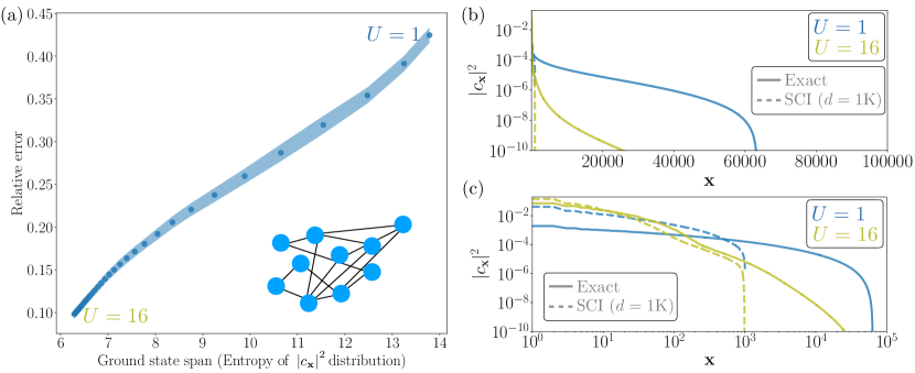
Fig. S3 (a) shows the relative error in the ground-state energy obtained by SCI as a function of the entropy of the distribution of the wavefunction amplitudes. The more concentrated the ground-state wavefunction (lower entropy), the lower the relative error becomes. As expected, the SCI-based eigensolver performs better for large deep in the Mott phase. For small in the metallic phase, the SCI trial wavefunction with does not have enough expressive power to accurately represent the ground state of the system, whose amplitudes anti-concentrate.
Panels (b) and (c) in Fig. S3 show a comparison between the exact and SCI wavefunction amplitudes ordered by their magnitude for (metal) and (Mott insulator). For more concentrated wavefunctions () the SCI amplitudes are in better agreement with the exact amplitudes. For the number of relevant electronic configurations in the exact wavefunction greatly exceeds the configurations that SCI is allowed to use, explaining the poor performance of SCI in the prediction of the ground-state energy as shown in Fig. S3 (a).
II.3 Energy-variance extrapolation
It is expected that the accuracy of the HPC quantum estimator (with or without configuration recovery) will increase as the number of configurations used for the subspace expansion is increased. However, the convergence of the ground-state properties with is not expected to follow any specific functional relation. Therefore, attempting to analyze the convergence as a function of is not well motivated. Instead, the different eigenstate approximations obtained for different values of and different batches of samples are used for an energy-variance extrapolation [48, 94, 95, 96, 97, 98]. Consider the approximate eigenstate , whose energy is given by , and consider the exact eigenstate energy . The difference between the approximate energy and ,
| (S57) |
vanishes linearly with the Hamiltonian variance divided by the square of the variational energy [48]
| (S58) |
This linear relation is satisfied as long as is sufficiently close to an eigenstate of the Hamiltonian, as measured by the state fidelity. The least squares fit of a collection of energy-variance points yields an estimate of , as the intersect of the fit with the ordinates. This point is the extrapolation of the estimate of the energy to the limit where coincides with the exact eigenstate. Besides the energy extrapolation, the energy-variance analysis may also reveal the existence of multiple eigenstates close in energy to the ground state.
In the main text and in this supplementary material we apply the energy-variance analysis to two different sets of energy-variance pairs. The first one is the energy-variance pairs obtained by the HCI procedure where different energies and variances are obtained by changing the cutoff parameter that indirectly controls the number of determinants in the subspace projection and diagonalization, resulting in different levels of accuracy. The second set of energy-variance pairs are those obtained from the HPC quantum estimator for different numbers of configurations as well as for different batches of sampled configurations .
III Experiments
This section begins by describing the quantum circuits that are employed to produce the configurations to which we apply the eigenstate solver. We describe how to set the circuit parameters from an efficient classical CCSD calculation, and show examples of the structure of the compiled circuits. We show numerical experiments comparing the performance of the circuits we use against the performance of a classically efficient reduction of the LUCJ circuits.
We also describe the setup for all of the experiments conducted in this work, highlighting the quantum and classical hardware used. We show the quantum device mappings, depth and number of gates in the circuits, and the number of measurement outcomes sampled. We also provide details about the classical computing resources.
III.1 Quantum circuits
In this work, we used the local-unitary cluster Jastrow (LUCJ) ansatz [40] to sample randomly distributed electronic configurations. LUCJ derives from the unitary cluster Jastrow (UCJ) ansatz, which has the form [41] of a product of layers,
| (S59) |
where
| (S60) |
In Eq. (S60), label molecular spatial orbitals and label spin polarizations ( for spin-up and spin-down electrons respectively). / has complex/real matrix elements and is anti-Hermitian/symmetric. The UCJ ansatz can be derived from a twice-factorized low-rank decomposition of the qUCCD ansatz [99, 41], and the -product form is such that the exact full configuration interaction wavefunction can be obtained via Eq. (S59) [41, 39].
The local UCJ or LUCJ [40] introduces a “local” approximation of the UCJ ansatz, which makes the following modifications for opposite-spin and same-spin number-number terms:
| (S61) |
where and the sets are such that the quantum circuit implementing has depth and only comprises number-number “nn gates,” i.e. two-qubit unitaries of the form , acting on adjacent qubits in the topology of a certain device. For example, on a heavy-hex device, and [40]. The circuits , on the other hand, can be implemented by a Bogolyubov circuit acting on qubits and comprising gates and depth [100, 101, 102]. Through the local approximation, the LUCJ Ansatz balances hardware friendliness and accuracy, the latter ultimately deriving from its connection to coupled cluster theory and adiabatic state preparation [40].
Unless otherwise specified, we use the truncated LUCJ circuit , which is the result of considering the two-layer LUCJ circuit and removing the last orbital rotation and last Jastrow operations. The resulting state is implemented by a circuit whose depth is identical to the single-layer LUCJ circuit. The addition of the operation to the circuit can have a large impact on the configurations generated by the circuit when the parameters are set from the tensor from a classical restricted closed-shell CCSD calculation (as described in the next section). For dynamically correlated species, the parameters obtained from can have a small amplitude, resulting in the approximate cancellation of the and terms in the ansatz. Without , the resulting wavefunction can be over-concentrated around the Hartree-Fock configuration. Therefore, for dynamically correlated species the action of is to remove some of the excessive concentration of the wavefunction, when parameters are set from a restricted closed-shell CCSD calculation.
III.1.1 Initialization of LUCJ parameters
In our experiments, we parametrize the LUCJ circuits using the following procedure:
-
1.
First, we carry out a classical restricted closed-shell CCSD calculation, yielding amplitudes and , where / labels occupied/unoccupied orbitals in the RHF state.
-
2.
We reshape the tensor into the matrix and diagonalize it, , where the eigenvectors are sorted in decreasing order of absolute value.
-
3.
We extend the unitaries to the following matrices,
(S62) i.e. matrices where only the occupied/unoccupied block is non-zero.
-
4.
We define the Hermitian operators
(S63) and their eigenpairs
(S64) -
5.
We define the operators
(S65) - 6.
-
7.
We zero out the entries of the matrices leading to quantum gates acting on non-adjacent qubits. For a heavy-hex lattice, we retain the following elements:
(S66)
The final sparsification allows us to construct a LUCJ wavefunction. In a conventional LUCJ calculation, these parameters are the starting point of a variational optimization. For the hardware experiments reported in this study, we employed these parameters, without further optimization, to define a LUCJ circuit, that we used to sample randomly distributed configurations.
III.1.2 Mapping to heavy-hex devices
The choice of retaining the elements with when implementing LUCJ on a heavy-hex device has an important technical motivation: on such devices, assuming a number of qubits greatly exceeding , spin-up and spin-down orbitals can be mapped on two segments of adjacent qubits forming a “zig-zag” pattern and connected through an auxiliary qubit for as shown in the three rightmost panels of Fig. S9. Such a qubit layout allows implementing LUCJ with a minimal overhead of gates (two per auxiliary qubit and layer of LUCJ). However, on current devices with up to 133 qubits, for one cannot couple spin-orbitals with opposite spins through auxiliary qubits without incurring a significant overhead of gates, for the simple reason that a chain of 22 or more qubits is longer than the “diagonal” of the device. In such a situation, as shown in the rightmost panel of Fig. S9, the segments on which spin-up and spin-down qubits are mapped form two “tails” that are not connected by auxiliary qubits. This fact has two implications: (i) no more than 6 spin-orbitals with opposite spins can be coupled through auxiliary qubits, and (ii) if one retains the elements with and , the largest elements of may be discarded, yielding a lower-accuracy wavefunction. The first problem is a fundamental one, that can only be resolved with a substantially different mapping of fermionic degrees of freedom onto qubits and/or through the availability of larger devices. The second problem, on the other hand, has a simple solution, that we now describe. First, for any pair of spatial orbitals , the orbital rotation
| (S67) |
implements the permutation exchanging orbitals and , in the sense that
| (S68) |
Three immediate implications of this fact are:
-
•
.
-
•
for any density-density operator , one has
(S69) -
•
that for any permutation there exists an orbital rotation implementing the permutation (this is true because permutations can be written as products of exchange permutations, an exchange permutation can be implemented by an orbital rotation, and orbital rotations are closed under multiplication).
Consider now the tensor resulting from the low-rank decomposition of the CCSD operator described in the previous Subsection. Let be the elements of with the largest absolute values, and let be the permutation such that . Then,
| (S70) |
where the elements of with the largest absolute values are at positions . Before sparsifying the tensor , one can use the identity
| (S71) |
to obtain a UCJ operator with transformed orbital rotations and an opposite-spin density-density interaction whose largest elements in absolute value act on spatial orbitals . Sparsification of then leads to retaining the dominant opposite-spin density-density interaction terms (as many as allowed by the size and topology of the available heavy-hex device) with a minimal overhead of gates.
In this work, we retained the elements with and . In future work, the procedure described here could be used to modify the LUCJ wavefunction and the resulting probability distribution for electronic configurations.
III.1.3 Compiled circuits
In Figures S4, S5, S6, and S7, we show the specific LUCJ circuits considered in this work. Each circuit is compiled into single-qubit
| (S72) |
and two-qubit gates. For readability, the displayed circuits contain barriers separating orbital rotations and density-density interactions, which we removed in the final compilation to / to reduce circuit depth. It is worth noting that the leftmost part of the quantum circuit does not implement the Bogolyubov transformation , but prepares the Slater Determinant . In other words, it reproduces the action of on a specific Slater determinant, which allows for a drastic reduction in circuit size without information loss. Subsequent orbital rotations are not amenable to such a circuit simplification.
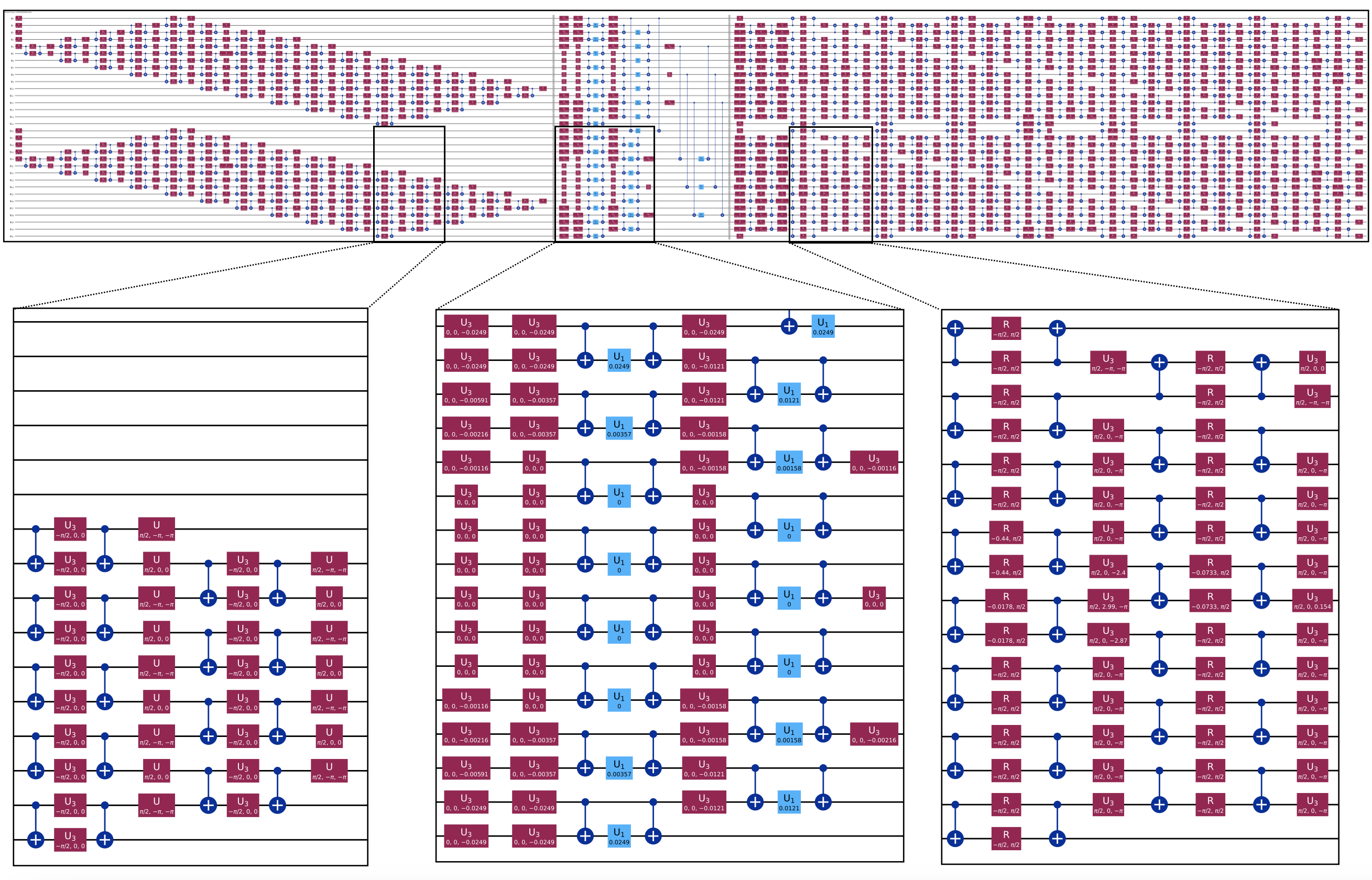
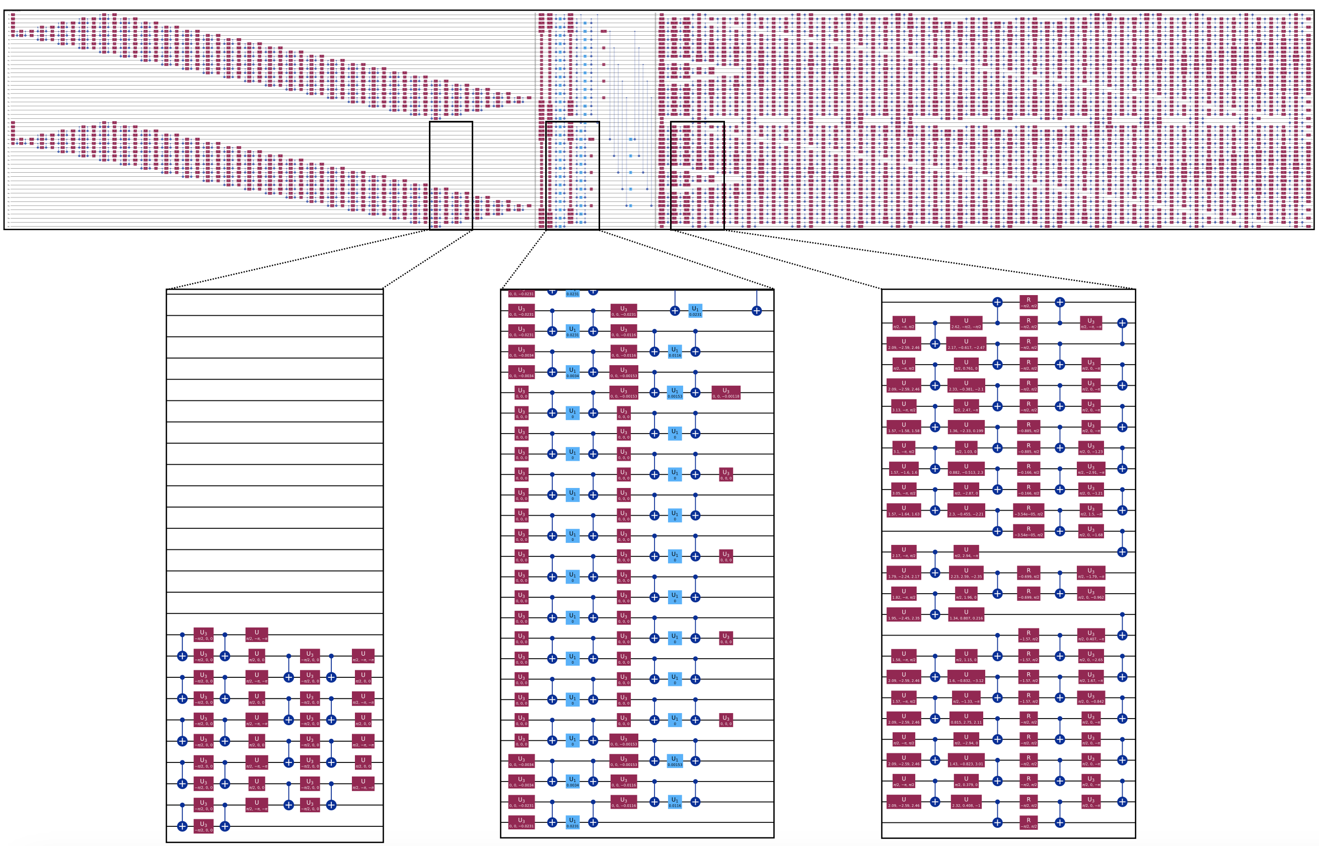
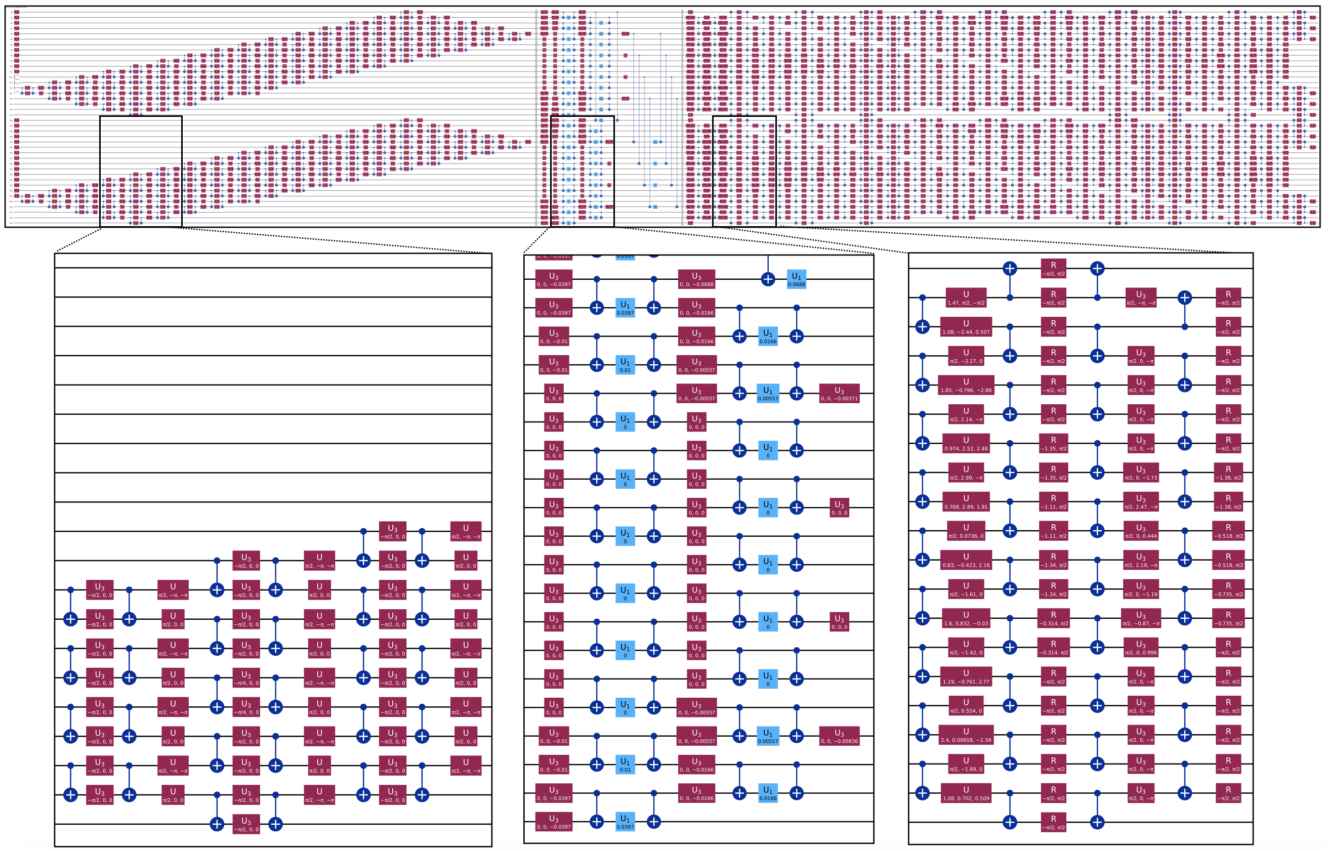
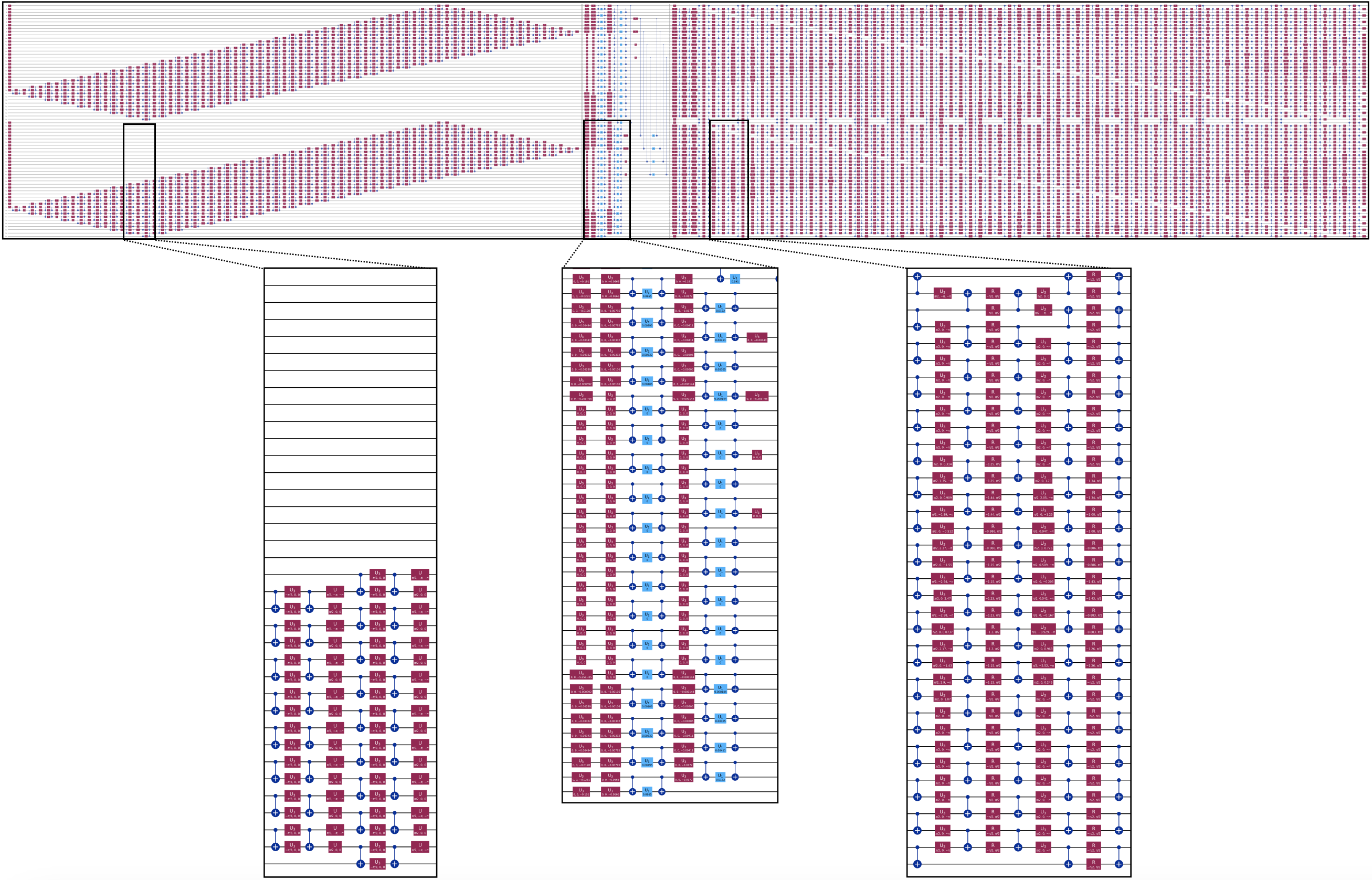
III.1.4 Effect of the Jastrow terms in the accuracy
In this section we study the impact of the two-body terms, , of the LUCJ ansatz in the performance of the HPC quantum estimator. We compare the case where the two-body parameters are zero, , against the most general case where they can take arbitrary real values. Without the density-density interactions, the remaining circuit is a free-fermion evolution, i.e. the wavefunction amplitudes remain those of a single Slater determinant [83], so it can be efficiently simulated by a classical computer.
We present a numerical study of that emulates the procedure without taking into account the effect of noise. Thus, there is no configuration recovery. For the quantum circuit simulations, we used the software library ffsim [42]. ffsim performs the state vector simulation within a subspace of fixed particle number and total component of the spin, making the simulations much more efficient than a generic quantum circuit simulator.
Three circuits are considered: LUCJ(), LUCJ(), and the LUCJ circuit without two-body terms, which we refer to as “Determinant”. We study the accuracy of the estimator in the dissociation of N2 (6-31G). For the LUCJ circuits, we consider those with heavy-hex-like connectivity in the density-density interactions; see Eq. (S66). The circuits are optimized to minimize the estimator energy, as described in Sec. II.1.3 using the COBYLA [70] optimizer. At each optimization step we consider batches of samples obtained from the set of sampled configurations , where . The value of at each point in the dissociation curve is chosen to coincide with the number of configurations resulting from a converged HCI calculation, carried out on PySCF, in the same system.
Fig. S8 (a) shows the potential energy surface obtained from the HPC quantum estimator run on configurations generated by LUCJ(), LUCJ() and the determinant circuits. Panel (b) in Fig. S8 shows the energy error from the three different circuits. For most bond lengths, the error of the HPC quantum estimator is largest for the determinant circuit, showing that the density-density interactions play a crucial role for the generation of relevant electronic configurations. This claim is also supported by the decrease of the error (on average) when increasing the number of LUCJ layers. We note that the optimization of the LUCJ circuits takes more iterations to converge than the optimization of the determinant circuits.
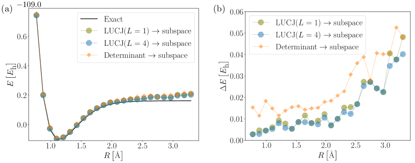
III.2 Quantum and classical computational resources
III.2.1 Quantum experiment details
This section provides technical details about the experiments carried out on the quantum devices. The circuits that we use come from the truncation of two layers of the LUCJ circuits (as described in Sec. III.1). For the quantum runs, the circuit parameters are not optimized and instead are obtained from a classical CCSD calculation, as described in Sec. III.1. Note that the circuits themselves are still classically challenging to simulate.
Table 2 lists the different molecular species, together with the number of qubits used to encode the that generates samples of electronic configurations. The same table also provides details about the total circuit depths, and numbers of one- and two-qubit gates, as well as the IBM device that was used to run the experiments. The specific qubit layouts are also provided in Table 2 and depicted in Fig. S9.
In the experiments that study the dissociation of N2 , the number of measurement outcomes collected is and per point in the dissociation curve at 6-31G and cc-pVDZ level of theory respectively. In the experiments to study the ground-state properties of [2Fe-2S] and [4Fe-4S], the number of measurement outcomes collected is . Out of the total number of measurement outcomes, a fraction of the configurations live in the subspace of the Fock space with the correct particle number, defined as
| (S73) |
Table 2 shows the 95% confidence interval for that fraction. Recall that the measurement outcomes that correspond to configurations with the correct particle number are used in the setup phase of the configuration recovery procedure. Table 2 also shows the fraction of sampled configurations with the correct particle number if samples were collected from the uniform distribution over configurations of length ,
| (S74) |
As shown in the Table, the two probabilities are statistically distinguishable for all the experiments we carried out. Our experiments used twirled readout error mitigation (ROEM) [103] to mitigate errors arising from qubit measurement, and dynamical decoupling (DD) [104, 105, 106, 107] to mitigate errors arising from quantum gates. We employed the implementation of ROEM and DD available on the Runtime library of Qiskit [108], through the Sampler primitive. DD is implemented by sequences of control pulses, whose effect is to protect qubits from decoherence due to low-frequency system-environment coupling. Here, we applied sequences of two pulses (as in Ramsey echo experiments) to idle qubits.
| system | q (JW, Tot.) | ( | device | layout | [95 c.i.] | ||
|---|---|---|---|---|---|---|---|
| N2, (10e,16o) | (32, 36) | (148,762,1408) | [082]+[273] | (0.0069,0.0071) | 0.0044 | ||
| N2, (10e,26o) | (52, 58) | (223,1792,3412) | [0121]+[2127] | (0.0016,0.0017) | |||
| [2Fe-2S], (30e,20o) | (40, 45) | (173,1100,2070) | [0104]+[294] | (0.0044,0.0045) | 0.00022 | ||
| [4Fe-4S], (54e,36o) | (72, 77) | (301,3590,6980) | [0100]+[228] | (,) |
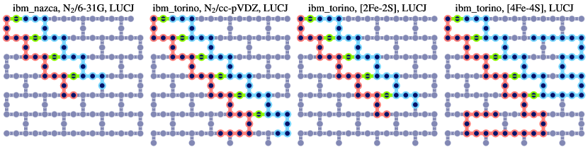
III.2.2 Classical resource details
The SCI-based eigenstate solver used by HPC quantum estimator is the one implemented in PySCF [26, 63] for the N2 (6-31G, cc-pVDZ), and [2Fe-2S] systems. For the [4Fe-4S] molecule we use the SCI-based eigenstate solver implemented in DICE [38, 35] because of its ability to run across multiple computer nodes.
For the [4Fe-4S] experiments, the eigenstate solver can be distributed across a number of classical nodes. The workflow for [4Fe-4S] is run on the supercomputer Fugaku. The supercomputer Fugaku has a total of 158,976 nodes with Armv8.2-A SVE 512 bit architecture. Each node has 82 cores and 32 GiB of memory. The largest calculation in this work uses 6400 nodes of the Fugaku supercomputer running in parallel.
IV Experimental results
This section contains the results from the experiments that are run on the quantum devices, as described in the previous section. We show a collection of investigations that are complementary to those shown in the main text.
We first visualize the prediction individual wave function components obtained by the HPC quantum estimator with configuration recovery in a system size where we have access to the exact ground state wave function amplitudes (N2 in the 6-31G basis).
We then study the scaling and runtime of the estimator. In particular, we study the effect and cost that more intensive classical resources have on the quality of the estimator. We choose the N2 (cc-pVDZ) and [2Fe-2S] molecules for this analysis.
We also study the effect of orbital optimizations in conjunction with the HPC quantum eigensolver in the quality of the predictions. We choose N2 in the cc-pVDZ basis as the case of study.
The results reported in Figure 4 of the main text, for the [2Fe-2S] cluster show the resolution of three different eigenstates. In this section we provide additional information about their nature. In particular, we study the average orbital occupancy for the three eigenstates in the MO and localized bases.
Lastly, we investigate the amount of signal that can be extracted and amplified from our experiments. For this study we consider the dissociation of N2 (cc-pVDZ) as well as the study of the low-energy spectrum of the [2Fe-2S] molecule. The same study for the [4Fe-4S] molecule is in the main text.
IV.1 Visualization of the wave function amplitudes
The aim of this subsection is to show the accuracy of individual wavefunction amplitudes obtained with the HPC quantum estimator (with configuration recovery). Configuration recovery is run on measurement outcomes obtained from a quantum device. We consider the dissociation of N2 in a basis set that is amenable to exact diagonalization techniques but larger than a minimal basis set: the 6-31G basis. The exact diagonalization wavefunction serves as the reference to asses the accuracy of the amplitudes produced by the estimator. For each point of the dissociation curve we collect measurement outcomes and run the configuration recovery procedure with batches of samples. The configuration recovery method is run for ten sefl-consistent iterations. The value of the subspace dimension for the SCI eigenstate solver is . For the potential energy surface we report . We show the amplitudes of the wavefunction from the batch of configurations whose energy is the lowest.
Panel (a) in Fig. S10 shows the potential energy surface of the molecule obtained by the estimator as well as the error in the estimation of the ground-state energy, as a function of the bond length. The error in the estimation of the ground-state energy remains below for all points in the dissociation curve, thus showing good agreement with the exact results.
Panel (b) in Fig. S10 shows a comparison between the exact ground state wavefunction amplitudes and the wavefunction amplitudes obtained by the estimator, for different points in the dissociation curve. The agreement is exceptional for the larger wavefunction amplitudes and slowly deteriorates in the description of the tails of the wavefunction. We also observe that for larger bond lengths, where higher levels of static correlation are present, the agreement in the tails is worse than for bond lengths closer to the equilibrium geometry. This is to be expected for two reasons. First, for larger bond lengths the wavefunction amplitudes are less concentrated than close to equilibrium. As discussed in Sec. II.2, the accuracy of the estimator using a SCI-based eigenstate solver deteriorates as the wavefunction becomes less concentrated. The second reason is that for bond lengths close to equilibrium, the wavefunction has a strong mean field character, but not for larger bond lengths. This directly impacts the shape of the reference spin-orbital occupancy that is used to recover configurations. When the wavefunction is mean-field dominated, takes the shape of a sharp step function shape with all spin-orbital average occupancies close to 0 or 1. One possible effect of static correlations is to soften the step function, moving average occupancies of some spin-orbitals away from 0 or 1. The recovery of configurations used in this work is more effective when the components of are close to 0 or 1.
In summary, the HPC quantum estimator with a SCI-based eigenstate solver and configuration recovery produces accurate representations of the ground state wavefunction (on experimental data), even at an individual amplitude level. Less concentrated wavefunctions tend to challenge the procedure more, both because the accuracy of the SCI solver is decreased, and because the configuration recovery becomes less effective due to softer profiles of .
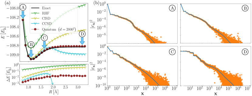
IV.2 Scaling and runtime
We begin this section by studying the improvement of the accuracy of the HPC quantum estimator with the number of determinants used for the subspace expansion and diagonalization. It is clear that larger yields more expressivity in the variational wavefunction, since we are increasing the possible size of the support of the state. It is also clear that increasing increases the HPC quantum estimator runtime since both the projection and diagonalization processes become more computationally intensive. To show the improvement of the accuracy with we consider the dissociation of N2 (cc-pVDZ), where the measurement outcomes are generated by the quantum device. The estimator is applied to measurement outcomes and we take batches of samples and report for the potential energy surface for different values of . Ten self-consistent iterations are considered for the recovery of configurations.
Fig. S11 shows the potential energy surfaces obtained by the estimator with different values of , the number of determinants used for the subspace expansion and diagonalization. Increasing the value of improves the results both qualitatively and quantitatively. For the smaller values of , the potential energy surface shows unphysical oscillations when the bond length is large. For larger values of , not only the energy values are lower, but also the oscillations in the energy as a function of the bond length are significantly decreased in amplitude. Improvement of the ground state approximation with an increasing amount of computational resources is also observed in the energy-variance analyses of the main text (Fig. 4), and the supplementary materials (Figs. S20 and S21).
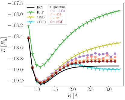
We analyze the vertical and horizontal scaling of the workflow, in the case where the subspace diagonalization is run on a single computer node, using the solver provided in the PySCF library. The [2Fe-2S] iron-sulfur cluster is used as the system of reference. Fig. S12 shows vertical scaling (increasing resources within a single node) of the eigenstate solver, and relative runtimes and schematics of horizontal scaling (adding nodes to cluster) of different blocks of the estimator (with configuration recovery). The eigenstate solver contributes the most to total runtime of the algorithm. Vertical scaling of the eigenstate solver shows noticable decrease in runtime up to a point. Experiments showed that for [2Fe-2S], 30+ CPUs per node is the optimal configuration. A good strategy for classical scaling would be to find the optimal vertical configuration and then scale horizontally for better utilization of resources.
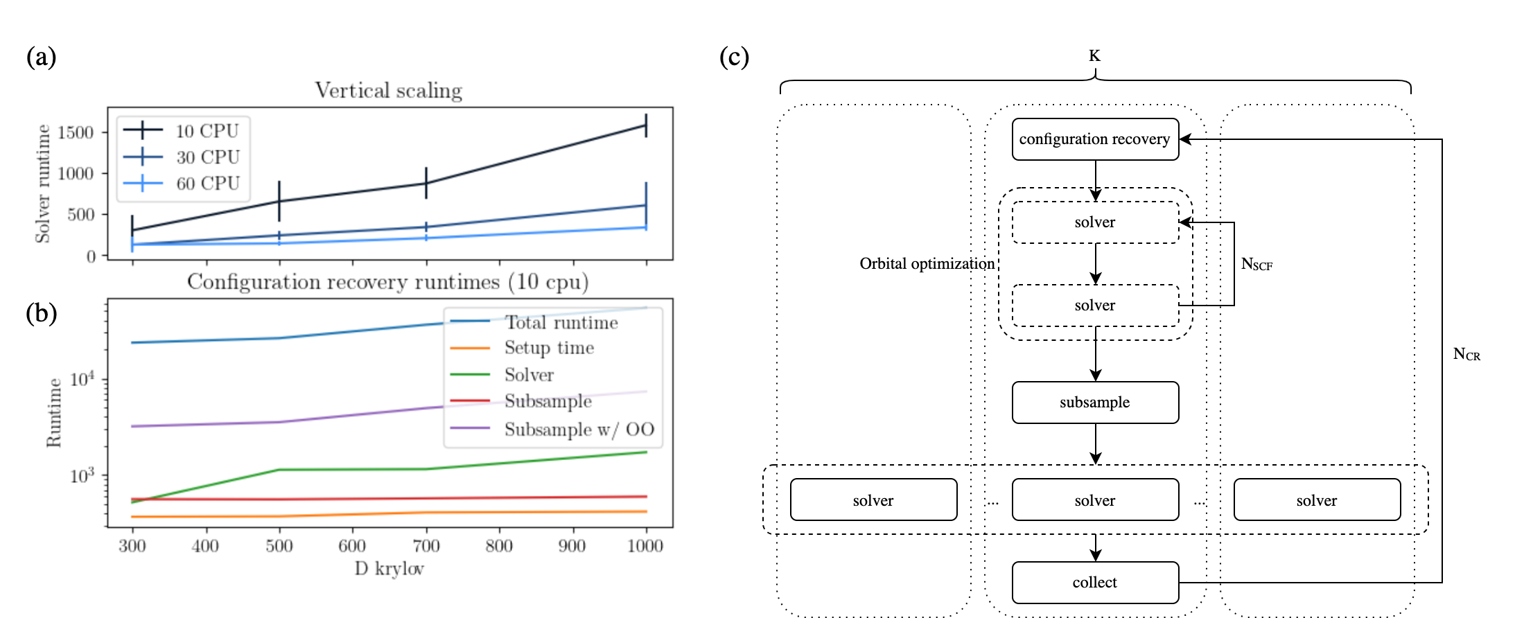
To conclude this section, we study the dependence of the runtime and accuracy of the estimator in the [4Fe-4S] system as a function of the amount of classical compute. The classical compute can be increased by increasing the size of the subspace dimension , or by collecting more batches of configurations . The DICE library allows to distribute the subspace diagonalization across a number of independent computer nodes. It is expected that more classical nodes will yield faster runtimes per diagonalization. For this experiment the Heron device Montecarlo is used, with collected measurement outcomes, and .
Fig. S13 (a) shows the runtime of the diagonalization of a single batch of configurations as a function of the number of classical nodes. Different subspace dimensions are considered. As expected, with an increased number of nodes, the runtime of the diagonalization decreases. After a certain number of nodes, the speedup saturates, due to the overhead in inter-node communications. This panel allows us to identify the number of classical nodes necessary to have a fixed runtime for the diagonalization for different subspace dimensions. To study improvement of the accuracy of the estimator with the number of batches of configurations , we run the workflow with . From the , batches, we subsample the energy of smaller groups of batches and collect the minimum energy for each subsample. The subsampled minimum energies are averaged. Different sizes of the smaller groups of batches are considered until reaching the group of batches of configurations. Panel (b) in Fig. S13 shows the average of the minimum energies as a function of the total number of nodes for different values of , such that the runtime of each digonalization is fixed to 1.44 hours. The total number of classical nodes is given by the product of the size of the groups of batches of configurations and the number of nodes required to obtain a runtime of 1.44 hours per subspace projection and diagonalization.
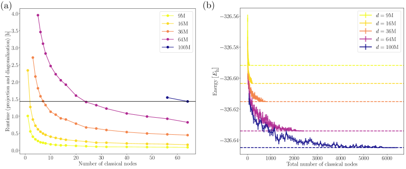
IV.3 Effect of orbital optimizations in the dissociation of N2 (cc-pVDZ)
We apply orbital optimizations (OO) to improve the accuracy of the HPC quantum estimator, in the study of the dissociation of N2 (cc-pVDZ). The estimator with configuration recovery and its orbital-optimized counterpart are applied to the same set of noisy measurement outcomes obtained from the quantum device. We use batches of samples in each case and iterations of the alternation between the optimization of and running of the eigenstate solver to update . After each update, iterations of gradient descent with momentum are used to optimize . Before applying orbital optimizations, the configuration recovery procedure is run for 10 iterations on the reference basis (molecular orbitals). Various sizes of the batches are considered.
Fig. S14 compares the ground-state energy obtained by the estimator without and with orbital optimizations. We observe that close to the equilibrium bond length the effect of the orbital optimizations is negligible. However, upon dissociation, the estimator with orbital optimizations obtains noticeably lower ground state energies. For smaller values of , the estimator without orbital optimizations shows unphysical oscillations in the potential energy surface. The orbital optimizations decrease the amplitude of those oscillations.
In summary, orbital optimizations allow finding the single-particle basis in which the estimator is most accurate, thus improving the quality of its predictions. Furthermore, the optimization of the circuit parameters would allow the circuit to respond to the change of basis to produce electronic configurations better suited for the new basis. As mentioned earlier, the optimization of the circuit parameters will be the subject of follow-up projects. Note that the unrestricted optimization of can break symmetries that may be desirable to preserve, so it is up to the user to decide whether to use orbital optimizations or not.
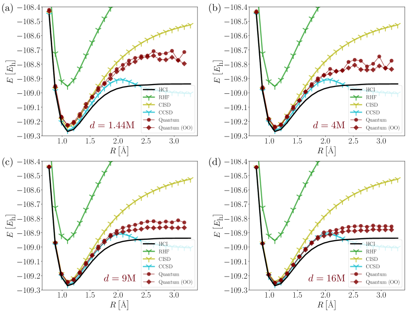
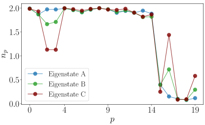
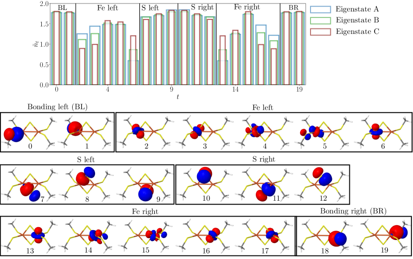
IV.4 Orbital occupation numbers for the low-energy spectrum of [2Fe-2S]
The calculations reported in Figure 4 of the main text, for the [2Fe-2S] cluster, identified three distinct eigenstates that we labeled A, B, and C. In this section, we provide additional information about the nature of the three identified eigenstates. The purpose of this analysis is to illustrate the robust classification of the wavefunctions produced by our estimator into three families (A, B, and C) but also to shed light on the nature of the corresponding eigenstates and the ability of our method to accurately capture a multireference character in electronic eigenstates, pinpointing areas of possible future improvement. In particular, we show the spatial orbital occupancy for the three eigenstates that the HPC quantum estimator finds for [2Fe-2S] both in the MO basis and in a basis of spatially local orbitals. The MO basis helps highlight deviations from the mean-field states or lack thereof, and the basis of localized orbitals (identifiable with e.g. Fe and S orbitals) helps characterize our method’s ability to capture local antiferromagnetic correlations between transition-metal atoms.
The spatial orbital occupancy is given by . Therefore . For Eigenstate A, the occupancy comes from the estimator run with . For Eigenstates B and C, the occupancy comes from the estimator run with . We cannot compare the occupancy for the same value of since the description of eigenstates A and B require different numbers of configurations (see Sec. IV.5.2 and Fig. S21). For Eigenstates B and C, we use the same number of determinants to make the comparison as even as possible. The number of batches of configurations is .
Fig. S15 shows the profile for the three eigenstates identified from the energy-variance analysis, in the basis of MOs. The occupancy profile for Eigenstate A is the typical profile of an eigenstate with a strong mean-field character. The occupancy of the lowest-energy molecular orbitals is close to its maximum value, while the remaining orbitals have lower occupancy. The character of the occupancy profile for Eigenstate B is different from that of Eigenstate A. The occupancy of the third and fourth orbitals is depleted to give a more prevalent presence of electrons in orbitals and . This effect is even more noticeable for eigenstate C, where the occupancy of the third and fourth orbitals is depleted by half and the occupancy of orbital is now over the half-filling factor.
To further understand the nature of Eigenstates B and C, we study the occupancy in the basis of localized orbitals (see Sec. I.2 for details about the basis of localized orbitals). The reported occupancies are constructed as follows: first, we obtain the one-body density matrix for the approximate ground state obtained from each batch of configurations, expressed in the basis of MOs: (see Eq. S40). We then rotate the density matrix to the basis of localized orbitals with a similarity transformation denoted by ,
| (S75) |
where is the one-body density matrix in the basis of localized orbitals. The occupancy of localized orbital is given by
| (S76) |
Fig. S16 shows a comparison of the value of for Eigenstates A, B, and C. The reflection symmetry along the plane that separates the left and right sides of the molecule is broken for the three approximate eigenstates. This is highlighted by the observation that the occupancy of the equivalent orbitals for the two Fe atoms are not the same. We also observe that the occupancy of the bonding orbitals of the SCH3 groups and the occupancy of the orbitals of the S atoms is similar for the three eigenstates. The occupancy of the orbitals of Fe has the largest differences among the three different eigenstates. The more notable discrepancy in the d-orbitals of Fe may be a consequence of the fact that the low-energy physics of this molecule is dominated by the antiferromagnetic coupling of the electrons in the Fe orbitals [45, 4].
IV.5 Quantum signal in the experiments
In this section we assess the quality of the quantum signal for all our experiments, going beyond the [4Fe-4S] analysis presented in the main text.. Given the large circuit sizes of our experiments:
-
•
2Fe-2S: 40 qubits (not including auxiliary), 1100 two-qubit gates, 3170 total gates,
-
•
N2 : 52 qubits (not including auxiliary), 1792 two-qubit gates, 5204 total gates,
-
•
4Fe-4S: 72 qubits (not including auxiliary), 3590 two-qubit gates, 10570 total gates,
one should verify whether there is a useful signal coming out of the quantum circuits, comparing samples from and uniform random samples. We first investigate the fraction of sampled configurations that live in the correct particle sector and compare it to the fraction that would be obtained if the samples came from the uniform distribution . The values for alongside their 95% confidence interval, and are reported in Table 2. For the 40-, 52-, and 72-qubit experiments, we observe that is , , and times larger than respectively. This provides a first indication that configurations sampled from the quantum device contain a signal that is distinguishable from white noise.
The second set of tests that we conduct is the comparison of the ground-state energy obtained by the HPC quantum estimator with and without applying the configuration recovery procedure. Note that not applying configuration recovery makes the estimator equivalent to the QSCI framework [30] . Having reasonable energies (lower than or in the vicinity of the RHF energy) without applying configuration recovery reveals that the set already contains reasonable configurations to construct a non-random ground state.
The third set of tests involves comparing the performance of the HPC quantum estimator with configuration recovery run on configurations obtained from the quantum device and samples obtained from the uniform distribution. We consider the uniform distribution over all possible configurations in the Fock space, as well as the uniform distribution over configurations with the correct particle number, as in Fig. 4 (c) in the main text 111When considering samples from the uniform distribution over electronic configurations on the correct particle sector, the configuration recovery method cannot be applied since it only recovers configurations with the wrong particle number. Therefore, this scenario is equivalent to running QSCI (without configuration recovery) on those samples.. The results for these last two sets of tests are shown in the coming subsections for the 40-, 52- and 72-qubit experiments.
IV.5.1 N2 experiments
Effect of configuration recovery on the accuracy of the HPC quantum estimator.–
In this section, we compare the accuracy of the estimator without configuration recovery (applied to ) to the accuracy of the estimator with configuration recovery (applied to ). As for all N2 experiments, . From the experimental measurements, we observe that the average (over the bondlengths considered in this study) size of the set is . The maximum number of determinants that can be extracted to perform the projection and diagonalization is . Since typical values of used for the N2 molecule exceed we perform the projection and diagonalization using all the configurations obtained from (number of batches of configurations is ). For the estimator run with configuration recovery we use . In both cases, we report the energy for the potential energy surface. When running the estimator with configuration recovery we use 10 self-consistent recovery iterations.
Fig. S17 shows the comparison between the HPC quantum estimator run with and without configuration recovery. The ground-state energy is shown as a function of the bond length. The estimator run on , i.e. without configuration recovery, obtains energies comparable to RHF energies. A level of accuracy comparable to RHF is not desirable for correlated electronic structure methods. However, since no mitigation techniques have been used in the large circuits producing the samples, this is an indication that a useful quantum signal (mostly of mean-field character) is present in . As expected, the estimator with configuration recovery shows higher levels of accuracy as compared to not using configuration recoivery, obtaining a qualitatively correct dissociation curve upon increasing .
The accuracy of the energies obtained by the HPC quantum estimator without configuration recovery could be improved by obtaining more measurement outcomes and thus more configurations on the right particle sector. The typical values of used for the estimator with configuration recovery are larger than . With current noise rates, obtaining a larger size of to run the estimator without configuration recovery, requires the collection of many more measurement outcomes, at an efficiency where approximately only 1 in 1000 measured configurations has the right particle number (see Tab 2 for the precise fraction). Configuration recovery allows improving the accuracy of the HPC quantum estimator without the collection of more measurement outcomes from the quantum device. This is desirable as it reduces the overall cost of the calculation.
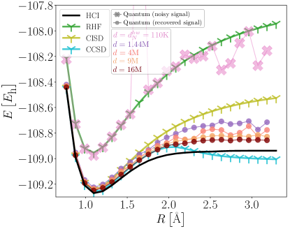
Comparison of the quality of the estimator with configuration recovery, applied to quantum data and configurations drawn from the uniform distribution.–
We first compare the performance of the estimator with configuration recovery applied to measurement outcomes from the quantum device versus its application to configurations sampled from the uniform distribution in the right particle sector. The estimator is applied to samples in both scenarios and we use the same value of . In both cases, we take batches of samples and report for the potential energy surface. When running the estimator with configuration recovery we use 10 self-consistent iterations. Recall that the configuration recovery procedure recovers configurations that have the wrong particle number due to noise, thus the application of the estimator to configurations sampled from the uniform distribution in the right particle sector is equivalent to applying the SCI eigenstate solver to the random configurations. Panel (a) in Fig. S18 shows the comparison. We observe that the potential energy surface obtained from the measurement outcomes from the quantum device is both qualitatively and quantitatively more accurate than the one obtained from the uniform distribution over configurations in the right particle sector. The potential energy surface obtained from the configurations sampled from the uniform distribution shows a very prominent non-smooth behavior with energies worse than the RHF energies for a number of bond lengths.
The comparison with samples obtained from the configurations uniformly sampled over the full Fock space and the quantum samples is shown in Fig. S18 (b). We remark that samples over the uniform distribution in the Fock space of electronic configurations are unlikely to reveal any configurations in the correct particle sector, since the probability of a uniformly random bitstring falling in the correct particle sector is . Recall that the configurations on the right particle sector are required to start the configuration recovery procedure by providing the initial average occupancies. Therefore, we take configurations sampled from the uniform distribution over configurations of length for this comparison. Note that the use of more samples from the uniform distribution as compared to the number of measurement outcomes from quantum constitutes a comparison that favors the uniform distribution scenario.
In spite of this, Fig. S18 (b) shows a higher level of accuracy obtained by the estimator with configuration recovery run using measurement outcomes from the quantum device. These results indicate that the quantum device has a signal that is amplified by the configuration recovery procedure and used by the HPC quantum estimator to procedure more accurate ground-state representations than running the same estimator on uniform noise.
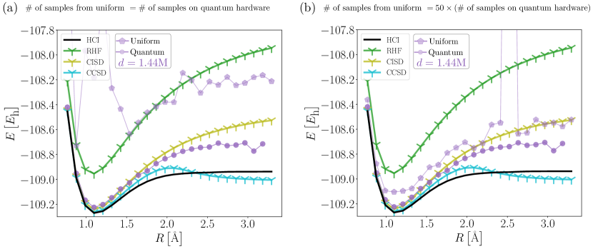
IV.5.2 [2Fe-2S] experiments
Effect of configuration recovery on the accuracy of the HPC quantum estimator.–
In this section, we compare the accuracy of the estimator without configuration recovery (i.e., applied to ) to the accuracy of the estimator with configuration recovery (applied to ). As for all [2Fe-2S] experiments, . In both cases, we take batches of samples. When running the configuration recovery procedure, we use 10 self-consistent recovery iterations.
Fig. S19 shows the Kernel Density Estimation (KDE) of the distribution running the HPC quantum estimator both with and without configuration recovery for different values of . The qualitative behavior of the KDE for the estimator with and without vonfiguration recovery is similar. Upon increasing the value of , the distributions shift towards lower values of the energy. However, the distributions of for the estimator with configuraiton recovery have lower energy than those without. Without configuration recovery, the best ground-state energy obtained is between the RHF and CISD energies, whereas when using the configuration recovery procedure, the energy is decreased even below the CCSD estimate. Again, note that the fact that the estimator without configuration recovery still has energies below RHF is a promising indication that the raw data from the device contains a signal that the configuration recovery procedure can amplify.
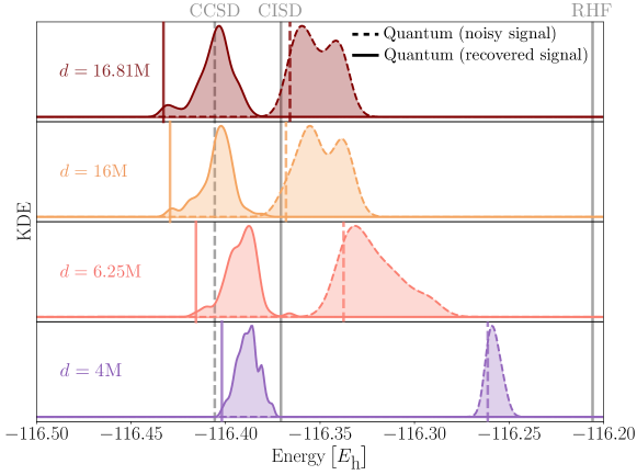
Comparison of the quality of the estimator with configuration recovery, applied to quantum data and configurations drawn from the uniform distribution.–
We first compare the performance of the HPC quantum estimator with configuration recovery applied to measurement outcomes from the quantum device versus configurations drawn from the uniform distribution over configurations in the right particle sector. In both cases we consider batches of electronic configurations and the estimator is applied to sampled configurations. The self-consistent recovery procedure is warm-started from the orbital occupancy vector obtained after running ten self-consitent iterations with . Since the configuration recovery is warm-started, for we apply two self-consistent iterations. In both scenarios, the same values of are considered. Recall that configuration recovery procedure recovers configurations that have the wrong particle number due to noise, thus the application of the estimator to configurations sampled from the uniform distribution in the right particle sector is equivalent to applying the SCI eigenstate solver to the random configurations. Fig. S20 shows a comparison of the energy-variance analysis obtained from the estimator on measurement outcomes from the quantum device and on uniformly random configurations with the right particle number. When the configurations come from measurement outcomes from a quantum device, the energy-variance analysis shows two clusters of points following a linear relation. The two clusters correspond to two eigenstates of the Hamiltonian. The extrapolated energy is in good agreement with the energy extrapolation from HCI calculations. The energy-variance analysis on the estimator run on the random configurations with the right particle number shows a different behavior. The energy-variance pairs are not clustered as clearly as in the previous scenario. For the largest values of considered, we observe that a first cluster begins to form, which coincides with the eigenstate of the highest energy that both HCI and the HPC quantum estimator applied to quantum measurement outcomes reveal. However, for these values of the HPC estimator run on random samples is not capable of revealing the second eigenstate of lower energy that the estimator run on quantum data obtains.
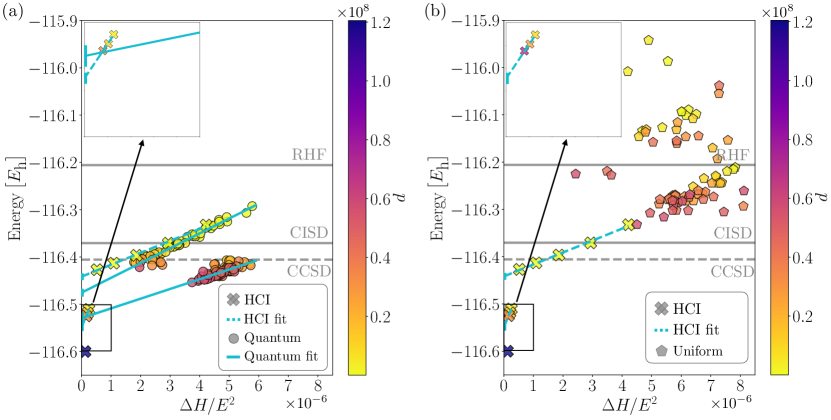
We also compare the performance of the HPC estimator with configuration recovery run on the data obtained from the quantum device versus on configurations drawn from the uniform distribution over the full Fock space. In both cases, we consider batches of electronic configurations and the estimator is applied to sampled configurations . The self-consistent recovery procedure is warm-started from the orbital occupancy vector obtained after running ten configuration recovery iterations with . Since the configuration recovery procedure is warm-started, for we apply two self-consistent operations. Fig. S21 (a) shows the comparison of the energy-variance analyses in both scenarios for values of the subspace dimension up to . The qualitative behavior is similar, showing a cluster of points following a line that coincides with Eigenstate A of the Hamiltonian. However, is enough for the estimator run on quantum samples to reveal the second cluster corresponding to Eigenstate B, while greater values of are required in the case where the samples are obtained from the uniform distribution over the full Fock space. Being able to resolve eigenstates of lower energy with smaller values of shows a more efficient description of the low-energy physics of the problem.
To quantify more precisely for which value of the Eigenstate B cluster of energy-variance pairs appears, we study the evolution of as a function of . A jump in reveals the discovery of a cluster in the energy-variance plane. Fig. S21 (b) shows the as a function of in both scenarios. While a large enough value of allows resolving Eigenstate B from the estimator with configuration recovery applied to the uniformly random samples, this transition requires the projection and diagonalization of the Hamiltonian in a subspace whose dimension is . The observation of the same transition on the configurations sampled from the quantum device requires at most configurations. The difference in these dimensions is of at least 3.75M electronic configurations.
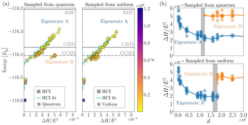
These results indicate that the quantum device provides a useful signal that is used by the HPC quantum estimator to procedure more accurate ground-state representations than using the same estimator on samples from uniform distribution.
References
- Feynman [1982] R. P. Feynman, Simulating physics with computers, Int. J. Theor. Phys 21, 467 (1982).
- Aspuru-Guzik et al. [2005] A. Aspuru-Guzik, A. D. Dutoi, P. J. Love, and M. Head-Gordon, Simulated quantum computation of molecular energies, Science 309, 1704 (2005).
- Wecker et al. [2015] D. Wecker, M. B. Hastings, and M. Troyer, Progress towards practical quantum variational algorithms, Phys. Rev. A 92, 042303 (2015).
- Sharma et al. [2014] S. Sharma, K. Sivalingam, F. Neese, and G. K.-L. Chan, Low-energy spectrum of iron-sulfur clusters directly from many-particle quantum mechanics, Nat. Chem 6, 927 (2014).
- Vogiatzis et al. [2017] K. D. Vogiatzis, D. Ma, J. Olsen, L. Gagliardi, and W. A. De Jong, Pushing configuration-interaction to the limit: towards massively parallel MCSCF calculations, J. Chem. Phys 147, 184111 (2017).
- Gao et al. [2024] H. Gao, S. Imamura, A. Kasagi, and E. Yoshida, Distributed implementation of full configuration interaction for one trillion determinants, J. Chem. Theory Comput (2024).
- LeBlanc et al. [2015] J. P. LeBlanc, A. E. Antipov, F. Becca, I. W. Bulik, G. K.-L. Chan, C.-M. Chung, Y. Deng, M. Ferrero, T. M. Henderson, C. A. Jiménez-Hoyos, et al., Solutions of the two-dimensional Hubbard model: benchmarks and results from a wide range of numerical algorithms, Phys. Rev. X 5, 041041 (2015).
- Motta et al. [2017] M. Motta, D. M. Ceperley, G. K.-L. Chan, J. A. Gomez, E. Gull, S. Guo, C. A. Jiménez-Hoyos, T. N. Lan, J. Li, F. Ma, et al., Towards the solution of the many-electron problem in real materials: equation of state of the hydrogen chain with state-of-the-art many-body methods, Phys. Rev. X 7, 031059 (2017).
- Cao et al. [2019] Y. Cao, J. Romero, J. P. Olson, M. Degroote, P. D. Johnson, M. Kieferová, I. D. Kivlichan, T. Menke, B. Peropadre, N. P. Sawaya, et al., Quantum chemistry in the age of quantum computing, Chem. Rev 119, 10856 (2019).
- McArdle et al. [2020] S. McArdle, S. Endo, A. Aspuru-Guzik, S. C. Benjamin, and X. Yuan, Quantum computational chemistry, Rev. Mod. Phys 92, 015003 (2020).
- Bauer et al. [2020] B. Bauer, S. Bravyi, M. Motta, and G. Kin-Lic Chan, Quantum algorithms for quantum chemistry and quantum materials science, Chem. Rev 120, 12685 (2020).
- Kandala et al. [2017] A. Kandala, A. Mezzacapo, K. Temme, M. Takita, M. Brink, J. M. Chow, and J. M. Gambetta, Hardware-efficient variational quantum eigensolver for small molecules and quantum magnets, Nature 549, 242 (2017).
- Google AI Quantum and Collaborators [2020] Google AI Quantum and Collaborators, Hartree-Fock on a superconducting qubit quantum computer, Science 369, 1084 (2020).
- Huggins et al. [2022] W. J. Huggins, B. A. O’Gorman, N. C. Rubin, D. R. Reichman, R. Babbush, and J. Lee, Unbiasing fermionic quantum Monte Carlo with a quantum computer, Nature 603, 416 (2022).
- Motta et al. [2023a] M. Motta, G. O. Jones, J. E. Rice, T. P. Gujarati, R. Sakuma, I. Liepuoniute, J. M. Garcia, and Y.-y. Ohnishi, Quantum chemistry simulation of ground- and excited-state properties of the sulfonium cation on a superconducting quantum processor, Chem. Sci 14, 2915 (2023a).
- Zhao et al. [2023] L. Zhao, J. Goings, K. Shin, W. Kyoung, J. I. Fuks, J.-K. Kevin Rhee, Y. M. Rhee, K. Wright, J. Nguyen, J. Kim, et al., Orbital-optimized pair-correlated electron simulations on trapped-ion quantum computers, npj Quantum Inf 9, 60 (2023).
- Google AI Quantum and Collaborators [2023] Google AI Quantum and Collaborators, Purification-based quantum error mitigation of pair-correlated electron simulations, Nat. Phys 19, 1787 (2023).
- Weaving et al. [2023] T. Weaving, A. Ralli, P. J. Love, S. Succi, and P. V. Coveney, Contextual subspace variational quantum eigensolver calculation of the dissociation curve of molecular nitrogen on a superconducting quantum computer (2023), arXiv:2312.04392 [quant-ph] .
- Verteletskyi et al. [2020] V. Verteletskyi, T.-C. Yen, and A. F. Izmaylov, Measurement optimization in the variational quantum eigensolver using a minimum clique cover, J. Chem. Phys 152, 124114 (2020).
- Huggins et al. [2021] W. J. Huggins, J. R. McClean, N. C. Rubin, Z. Jiang, N. Wiebe, K. B. Whaley, and R. Babbush, Efficient and noise resilient measurements for quantum chemistry on near-term quantum computers, npj Quantum Inf 7, 1 (2021).
- Dutt et al. [2023] A. Dutt, W. Kirby, R. Raymond, C. Hadfield, S. Sheldon, I. L. Chuang, and A. Mezzacapo, Practical benchmarking of randomized measurement methods for quantum chemistry Hamiltonians, arXiv:2312.07497 (2023).
- Anand et al. [2022] A. Anand, P. Schleich, S. Alperin-Lea, P. W. Jensen, S. Sim, M. Díaz-Tinoco, J. S. Kottmann, M. Degroote, A. F. Izmaylov, and A. Aspuru-Guzik, A quantum computing view on unitary coupled cluster theory, Chem. Soc. Rev 51, 1659 (2022).
- Hastings et al. [2015] M. B. Hastings, D. Wecker, B. Bauer, and M. Troyer, Improving quantum algorithms for quantum chemistry, Quant. Info. Comput 15, 1–21 (2015).
- Lee et al. [2021] J. Lee, D. W. Berry, C. Gidney, W. J. Huggins, J. R. McClean, N. Wiebe, and R. Babbush, Even more efficient quantum computations of chemistry through tensor hypercontraction, Phys. Rev. X Quantum 2, 030305 (2021).
- Alexeev et al. [2023] Y. Alexeev, M. Amsler, P. Baity, M. A. Barroca, S. Bassini, T. Battelle, D. Camps, D. Casanova, F. T. Chong, C. Chung, et al., Quantum-centric supercomputing for materials science: A perspective on challenges and future directions, arXiv preprint arXiv:2312.09733 (2023).
- Sun et al. [2018] Q. Sun, T. C. Berkelbach, N. S. Blunt, G. H. Booth, S. Guo, Z. Li, J. Liu, J. D. McClain, E. R. Sayfutyarova, S. Sharma, et al., PySCF: the python-based simulations of chemistry framework, WIREs Comput. Mol. Sci 8, e1340 (2018).
- Jordan and Wigner [1928] P. Jordan and E. Wigner, Über das paulische äquivalenzverbot, Zeit. Phys 47, 631 (1928).
- Ivanic and Ruedenberg [2001] J. Ivanic and K. Ruedenberg, Identification of deadwood in configuration spaces through general direct configuration interaction, Theor. Chem. Acc 106, 339 (2001).
- [29] See supplementary information.
- Kanno et al. [2023] K. Kanno, M. Kohda, R. Imai, S. Koh, K. Mitarai, W. Mizukami, and Y. O. Nakagawa, Quantum-selected configuration interaction: classical diagonalization of Hamiltonians in subspaces selected by quantum computers (2023), arXiv:2302.11320 [quant-ph] .
- Nakagawa et al. [2023] Y. O. Nakagawa, M. Kamoshita, W. Mizukami, S. Sudo, and Y. ya Ohnishi, ADAPT-QSCI: Adaptive construction of input state for quantum-selected configuration interaction (2023), arXiv:2311.01105 [quant-ph] .
- Evangelista [2014] F. A. Evangelista, Adaptive multiconfigurational wave functions, J. Chem. Phys 140, 124114 (2014).
- Schriber and Evangelista [2016] J. B. Schriber and F. A. Evangelista, Communication: An adaptive configuration interaction approach for strongly correlated electrons with tunable accuracy, J. Chem. Phys 144, 161106 (2016).
- Holmes et al. [2016a] A. A. Holmes, H. J. Changlani, and C. Umrigar, Efficient heat-bath sampling in Fock space, J. Chem. Theory Comput 12, 1561 (2016a).
- Holmes et al. [2016b] A. A. Holmes, N. M. Tubman, and C. Umrigar, Heat-bath configuration interaction: An efficient selected configuration interaction algorithm inspired by heat-bath sampling, J. Chem. Theory Comput 12, 3674 (2016b).
- Tubman et al. [2016] N. M. Tubman, J. Lee, T. Y. Takeshita, M. Head-Gordon, and K. B. Whaley, A deterministic alternative to the full configuration interaction quantum Monte Carlo method, J. Chem. Phys 145, 044112 (2016).
- Schriber and Evangelista [2017] J. B. Schriber and F. A. Evangelista, Adaptive configuration interaction for computing challenging electronic excited states with tunable accuracy, J. Chem. Theory Comput 13, 5354 (2017).
- Sharma et al. [2017] S. Sharma, A. A. Holmes, G. Jeanmairet, A. Alavi, and C. J. Umrigar, Semistochastic heat-bath configuration interaction method: Selected configuration interaction with semistochastic perturbation theory, J. Chem. Theory Comput 13, 1595 (2017).
- Evangelista et al. [2019] F. A. Evangelista, G. K.-L. Chan, and G. E. Scuseria, Exact parameterization of fermionic wave functions via unitary coupled cluster theory, J. Chem. Phys 151, 244112 (2019).
- Motta et al. [2023b] M. Motta, K. J. Sung, K. B. Whaley, M. Head-Gordon, and J. Shee, Bridging physical intuition and hardware efficiency for correlated electronic states: the local unitary cluster Jastrow ansatz for electronic structure, Chem. Sci 14, 11213 (2023b).
- Matsuzawa and Kurashige [2020] Y. Matsuzawa and Y. Kurashige, Jastrow-type decomposition in quantum chemistry for low-depth quantum circuits, J. Chem. Theory Comput 16, 944 (2020).
- The ffsim developers [2024] The ffsim developers, ffsim: Faster simulations of fermionic quantum circuits (2024).
- Fan and Piecuch [2006] P.-D. Fan and P. Piecuch, The usefulness of exponential wave function expansions employing one-and two-body cluster operators in electronic structure theory: The extended and generalized coupled-cluster methods, Adv. Quantum Chem 51, 1 (2006).
- Bulik et al. [2015] I. W. Bulik, T. M. Henderson, and G. E. Scuseria, Can single-reference coupled cluster theory describe static correlation?, J. Chem. Theory Comput 11, 3171 (2015).
- Li and Chan [2017a] Z. Li and G. K.-L. Chan, Spin-projected matrix product states: versatile tool for strongly correlated systems, J. Chem. Theory Comput 13, 2681 (2017a).
- Beinert et al. [1997] H. Beinert, R. H. Holm, and E. Munck, Iron-sulfur clusters: nature’s modular, multipurpose structures, Science 277, 653 (1997).
- Venkateswara Rao and Holm [2004] P. Venkateswara Rao and R. Holm, Synthetic analogues of the active sites of iron-sulfur proteins, Chem. Rev 104, 527 (2004).
- Kashima and Imada [2001] T. Kashima and M. Imada, Path-integral renormalization group method for numerical study on ground states of strongly correlated electronic systems, J. Phys. Soc. Jpn 70, 2287 (2001).
- Papaefthymiou et al. [1986] V. Papaefthymiou, M. M. Millar, and E. Muenck, Moessbauer and EPR studies of a synthetic analog for the iron-sulfur Fe4S4 core of oxidized and reduced high-potential iron proteins, Inorg. Chem 25, 3010 (1986).
- Kim et al. [2023] Y. Kim, A. Eddins, S. Anand, K. X. Wei, E. Van Den Berg, S. Rosenblatt, H. Nayfeh, Y. Wu, M. Zaletel, K. Temme, et al., Evidence for the utility of quantum computing before fault tolerance, Nature 618, 500 (2023).
- Shinjo et al. [2024] K. Shinjo, K. Seki, T. Shirakawa, R.-Y. Sun, and S. Yunoki, Unveiling clean two-dimensional discrete time quasicrystals on a digital quantum computer, arXiv preprint arXiv:2403.16718 (2024).
- Reardon-Smith et al. [2023] O. Reardon-Smith, M. Oszmaniec, and K. Korzekwa, Improved simulation of quantum circuits dominated by free fermionic operations, arXiv preprint arXiv:2307.12702 (2023).
- Lee et al. [2023] S. Lee, J. Lee, H. Zhai, Y. Tong, A. M. Dalzell, A. Kumar, P. Helms, J. Gray, Z.-H. Cui, W. Liu, et al., Evaluating the evidence for exponential quantum advantage in ground-state quantum chemistry, Nat. Commun 14, 1952 (2023).
- Becca and Sorella [2017] F. Becca and S. Sorella, Quantum Monte Carlo approaches for correlated systems (Cambridge University Press, 2017).
- Carleo and Troyer [2017] G. Carleo and M. Troyer, Solving the quantum many-body problem with artificial neural networks, Science 355, 602 (2017).
- White and Martin [1999] S. R. White and R. L. Martin, Ab initio quantum chemistry using the density matrix renormalization group, J. Chem. Phys 110, 4127 (1999).
- Chan and Sharma [2011] G. K.-L. Chan and S. Sharma, The density matrix renormalization group in quantum chemistry, Annu. Rev. Phys. Chem 62, 465 (2011).
- Hubig et al. [2018] C. Hubig, J. Haegeman, and U. Schollwöck, Error estimates for extrapolations with matrix-product states, Phys. Rev. B 97, 045125 (2018).
- Li et al. [2019] Z. Li, J. Li, N. S. Dattani, C. Umrigar, and G. K. Chan, The electronic complexity of the ground-state of the FeMo cofactor of nitrogenase as relevant to quantum simulations, J. Chem. Phys 150, 024302 (2019).
- Hehre et al. [1969] W. J. Hehre, R. F. Stewart, and J. A. Pople, Self-consistent molecular-orbital methods. I. use of Gaussian expansions of Slater-type atomic orbitals, J. Chem. Phys 51, 2657 (1969).
- Hehre et al. [1972] W. J. Hehre, R. Ditchfield, and J. A. Pople, Self-consistent molecular orbital methods. XII. Further extensions of Gaussian-type basis sets for use in molecular orbital studies of organic molecules, J. Chem. Phys 56, 2257 (1972).
- Dunning [1989] T. H. Dunning, Gaussian basis sets for use in correlated molecular calculations. I. The atoms boron through neon and hydrogen, J. Chem. Phys 90, 1007 (1989).
- Sun et al. [2020] Q. Sun, X. Zhang, S. Banerjee, P. Bao, M. Barbry, N. S. Blunt, N. A. Bogdanov, G. H. Booth, J. Chen, Z.-H. Cui, et al., Recent developments in the PySCF program package, J. Chem. Phys 153, 024109 (2020).
- Becke [1988] A. D. Becke, Density-functional exchange-energy approximation with correct asymptotic behavior, Phys. Rev. A 38, 3098 (1988).
- Perdew [1986] J. P. Perdew, Density-functional approximation for the correlation energy of the inhomogeneous electron gas, Phys. Rev. B 33, 8822 (1986).
- Jorge et al. [2009] F. Jorge, A. Canal Neto, G. Camiletti, and S. Machado, Contracted Gaussian basis sets for Douglas-Kroll-Hess calculations: estimating scalar relativistic effects of some atomic and molecular properties, J. Chem. Phys 130 (2009).
- Liu [2010] W. Liu, Ideas of relativistic quantum chemistry, Mol. Phys 108, 1679 (2010).
- Li et al. [2012] Z. Li, Y. Xiao, and W. Liu, On the spin separation of algebraic two-component relativistic Hamiltonians, J. Chem. Phys 137, 154114 (2012).
- Tang et al. [2021] H. L. Tang, V. Shkolnikov, G. S. Barron, H. R. Grimsley, N. J. Mayhall, E. Barnes, and S. E. Economou, Qubit-ADAPT-VQE: an adaptive algorithm for constructing hardware-efficient ansaatzes on a quantum processor, PRX Quantum 2, 020310 (2021).
- Powell [1994] M. J. D. Powell, A direct search optimization method that models the objective and constraint functions by linear interpolation, in Advances in Optimization and Numerical Analysis, edited by S. Gomez and J.-P. Hennart (Springer Netherlands, Dordrecht, 1994) pp. 51–67.
- Roos et al. [1980] B. O. Roos, P. R. Taylor, and P. E. Sigbahn, A complete active space SCF method (CASSCF) using a density matrix formulated super-CI approach, Chem. Phys 48, 157 (1980).
- Head-Gordon and Pople [1988] M. Head-Gordon and J. A. Pople, Optimization of wave function and geometry in the finite basis Hartree-Fock method, J. Phys. Chem 92, 3063 (1988).
- Werner and Knowles [1985] H.-J. Werner and P. J. Knowles, A second order multiconfiguration SCF procedure with optimum convergence, J. Chem. Phys 82, 5053 (1985).
- Olsen [2011] J. Olsen, The CASSCF method: A perspective and commentary, Int. J. Quantum Chem 111, 3267 (2011).
- Zgid and Nooijen [2008] D. Zgid and M. Nooijen, The density matrix renormalization group self-consistent field method: orbital optimization with the density matrix renormalization group method in the active space, J. Chem. Phys 128, 144116 (2008).
- Wu et al. [2022] A.-K. Wu, M. T. Fishman, J. Pixley, and E. Stoudenmire, Disentangling interacting systems with fermionic gaussian circuits: application to the single impurity Anderson model, arXiv:2212.09798 (2022).
- Wouters and Van Neck [2014] S. Wouters and D. Van Neck, The density matrix renormalization group for ab initio quantum chemistry, Eur. Phys. J. D 68, 272 (2014).
- Moreno et al. [2023] J. R. Moreno, J. Cohn, D. Sels, and M. Motta, Enhancing the expressivity of variational neural, and hardware-efficient quantum states through orbital rotations (2023), arXiv:2302.11588 [quant-ph] .
- Sokolov et al. [2020] I. O. Sokolov, P. K. Barkoutsos, P. J. Ollitrault, D. Greenberg, J. Rice, M. Pistoia, and I. Tavernelli, Quantum orbital-optimized unitary coupled cluster methods in the strongly correlated regime: can quantum algorithms outperform their classical equivalents?, J. Chem. Phys 152, 124107 (2020).
- Mizukami et al. [2020] W. Mizukami, K. Mitarai, Y. O. Nakagawa, T. Yamamoto, T. Yan, and Y.-y. Ohnishi, Orbital optimized unitary coupled cluster theory for quantum computer, Phys. Rev. Research 2, 033421 (2020).
- Bierman et al. [2023] J. Bierman, Y. Li, and J. Lu, Improving the accuracy of variational quantum eigensolvers with fewer qubits using orbital optimization, J. Chem. Theory Comput 19, 790 (2023).
- Smith et al. [2017] J. E. Smith, B. Mussard, A. A. Holmes, and S. Sharma, Cheap and near exact casscf with large active spaces, Journal of chemical theory and computation 13, 5468 (2017).
- Thouless [1960] D. Thouless, Stability conditions and nuclear rotations in the Hartree-Fock theory, Nuc. Phys 21, 225 (1960).
- Bradbury et al. [2018] J. Bradbury, R. Frostig, P. Hawkins, M. J. Johnson, C. Leary, D. Maclaurin, G. Necula, A. Paszke, J. VanderPlas, S. Wanderman-Milne, and Q. Zhang, JAX: composable transformations of Python+NumPy programs (2018).
- Chowdhury et al. [2022] D. Chowdhury, A. Georges, O. Parcollet, and S. Sachdev, Sachdev-Ye-Kitaev models and beyond: window into non-Fermi liquids, Rev. Mod. Phys. 94, 035004 (2022).
- Friedman and Levine [1997] B. Friedman and G. Levine, Configuration-interaction approach to the two-dimensional Hubbard model near half-filling, Phys. Rev. B 55, 9558 (1997).
- Louis et al. [1999] E. Louis, F. Guinea, M. P. López Sancho, and J. A. Vergés, Configuration-interaction approach to hole pairing in the two-dimensional Hubbard model, Phys. Rev. B 59, 14005 (1999).
- Schwarz et al. [2015] L. R. Schwarz, G. H. Booth, and A. Alavi, Insights into the structure of many-electron wave functions of mott-insulating antiferromagnets: The three-band Hubbard model in full configuration interaction quantum Monte Carlo, Phys. Rev. B 91, 045139 (2015).
- Dobrautz et al. [2019] W. Dobrautz, H. Luo, and A. Alavi, Compact numerical solutions to the two-dimensional repulsive Hubbard model obtained via nonunitary similarity transformations, Phys. Rev. B 99, 075119 (2019).
- Rozenberg et al. [1994] M. J. Rozenberg, G. Kotliar, and X. Y. Zhang, Mott-Hubbard transition in infinite dimensions. II, Phys. Rev. B 49, 10181 (1994).
- Georges et al. [1996] A. Georges, G. Kotliar, W. Krauth, and M. J. Rozenberg, Dynamical mean-field theory of strongly correlated fermion systems and the limit of infinite dimensions, Rev. Mod. Phys. 68, 13 (1996).
- Lee et al. [2017] S.-S. B. Lee, J. von Delft, and A. Weichselbaum, Doublon-holon origin of the subpeaks at the Hubbard band edges, Phys. Rev. Lett. 119, 236402 (2017).
- Gauvin-Ndiaye et al. [2023] C. Gauvin-Ndiaye, J. Tindall, J. R. Moreno, and A. Georges, Mott transition and volume law entanglement with neural quantum states (2023), arXiv:2311.05749 [cond-mat.str-el] .
- Kwon et al. [1998] Y. Kwon, D. M. Ceperley, and R. M. Martin, Effects of backflow correlation in the three-dimensional electron gas: Quantum Monte Carlo study, Phys. Rev. B 58, 6800 (1998).
- Imada and Kashima [2000] M. Imada and T. Kashima, Path-integral renormalization group method for numerical study of strongly correlated electron systems, J. Phys. Soc. Jpn 69, 2723 (2000).
- Nomura et al. [2017] Y. Nomura, A. S. Darmawan, Y. Yamaji, and M. Imada, Restricted Boltzmann machine learning for solving strongly correlated quantum systems, Phys. Rev. B 96, 205152 (2017).
- Sorella [2001] S. Sorella, Generalized Lanczos algorithm for variational quantum Monte Carlo, Phys. Rev. B 64, 024512 (2001).
- Mizusaki and Imada [2002] T. Mizusaki and M. Imada, Extrapolation method for shell model calculations, Phys. Rev. C 65, 064319 (2002).
- Motta et al. [2021] M. Motta, E. Ye, J. R. McClean, Z. Li, A. J. Minnich, R. Babbush, and G. K.-L. Chan, Low rank representations for quantum simulation of electronic structure, npj Quantum Inf 7, 1 (2021).
- Reck et al. [1994] M. Reck, A. Zeilinger, H. J. Bernstein, and P. Bertani, Experimental realization of any discrete unitary operator, Phys. Rev. Lett 73, 58 (1994).
- Clements et al. [2016] W. R. Clements, P. C. Humphreys, B. J. Metcalf, W. S. Kolthammer, and I. A. Walmsley, Optimal design for universal multiport interferometers, Optica 3, 1460 (2016).
- Jiang et al. [2018] Z. Jiang, K. J. Sung, K. Kechedzhi, V. N. Smelyanskiy, and S. Boixo, Quantum algorithms to simulate many-body physics of correlated fermions, Phys. Rev. Appl 9, 044036 (2018).
- Nation et al. [2021] P. D. Nation, H. Kang, N. Sundaresan, and J. M. Gambetta, Scalable mitigation of measurement errors on quantum computers, Phys. Rev. X Quantum 2, 040326 (2021).
- Viola and Lloyd [1998] L. Viola and S. Lloyd, Dynamical suppression of decoherence in two-state quantum systems, Phys. Rev. A 58, 2733 (1998).
- Kofman and Kurizki [2001] A. Kofman and G. Kurizki, Universal dynamical control of quantum mechanical decay: modulation of the coupling to the continuum, Phys. Rev. Lett 87, 270405 (2001).
- Biercuk et al. [2009] M. J. Biercuk, H. Uys, A. P. VanDevender, N. Shiga, W. M. Itano, and J. J. Bollinger, Optimized dynamical decoupling in a model quantum memory, Nature 458, 996 (2009).
- Niu and Todri-Sanial [2022] S. Niu and A. Todri-Sanial, Effects of dynamical decoupling and pulse-level optimizations on IBM quantum computers, IEEE Trans. Quantum Eng 3, 1 (2022).
- Qiskit contributors [2023] Qiskit contributors, Qiskit: An open-source framework for quantum computing (2023).
- Li and Chan [2017b] Z. Li and G. K.-L. Chan, Repository: Active space model for iron sulfur clusters (2017b).
- Note [1] When considering samples from the uniform distribution over electronic configurations on the correct particle sector, the configuration recovery method cannot be applied since it only recovers configurations with the wrong particle number. Therefore, this scenario is equivalent to running QSCI (without configuration recovery) on those samples.