Computing Chebyshev polynomials using the complex Remez algorithm
Abstract
We employ the generalized Remez algorithm, initially suggested by P. T. P. Tang, to perform an experimental study of Chebyshev polynomials in the complex plane. Our focus lies particularly on the examination of their norms and zeros. What sets our study apart is the breadth of examples considered, coupled with the fact that the degrees under investigation are substantially higher than those in previous studies where other methods have been applied. These computations of Chebyshev polynomials of high degrees reveal discernible patterns which allow for conjectures to be formulated based on abundant experimental evidence. The use of Tang’s algorithm allows for computations executed with precision, maintaining accuracy within quantifiable margins of error. Additionally, as a result of our experimental study, we propose what we believe to be a fundamental relationship between Chebyshev and Faber polynomials associated with a compact set.
1 Introduction
Let be a compact subset of the complex plane . Our focus is directed towards monic polynomials that exhibit minimal deviation from zero over the set . In other words, for any given positive integer we want to find coefficients satisfying
| (1) |
The existence of minimizing coefficients is guaranteed through a compactness argument. However, such a minimizer does not need to be unique. If is a finite points set consisting of points then there are an infinite number of different minimizing polynomials. This is the only exceptional case and the assumption that consists of infinitely many points ensures the uniqueness of a monic minimizer of (1) for any which henceforth is denoted by . This is the so-called Chebyshev polynomial of degree corresponding to the set . For basic theory detailing the proofs of existence and uniqueness of Chebyshev polynomials we refer the reader to [2, 7, 9, 36, 25, 41].
Throughout this text we reserve the notation to denote the maximum norm on and let denote the open unit disk and the unit circle.
Historically the consideration of polynomial minimizers with respect to the maximum norm originate from the studies of P. L. Chebyshev who considered minimization on , see [6]. Chebyshev polynomials corresponding to real sets have been much better understood than the corresponding complex ones. The reason for this discrepancy in understanding can partially be attributed to the powerful alternation theorem which is valid for real Chebyshev polynomials, [7, p. 75]. For any compact set containing at least points the Chebyshev polynomial is characterized by having an alternating set on consisting of points. That is to say, there are points all contained in such that
| (2) |
This alternating property, whose analogue can be shown for general real approximation tasks, constitutes the theoretical grounding for the classical Remez algorithm which is used to compute real-valued best approximations, see [7, 25, 34, 35].
1.1 Chebyshev polynomials in the complex plane
Alternation fails to characterise Chebyshev polynomials for general complex sets . Apart from the fact that the argument of a Chebyshev polynomial at an extremal point can be any angle, not just with , the number of extremal points corresponding to on can vary greatly. While there are at least such extremal points on , see e.g. [41, Theorem 1, p. 446], there is no upper bound on the number of extremal points. Indeed, as the example shows, the entire sets may consist of extremal points of the Chebyshev polynomial.
One approach to studying Chebyshev polynomials in the complex plane comes from the fruitful interplay between approximation theory and potential theory. For this reason, we recall that to any compact set we can associate a quantity referred to as the logarithmic capacity, denoted , see [33, §5.1].
In [44] Szegő proved that
| (3) |
A recent proof of this fundamental inequality can be found in [33, Theorem 5.5.4]. Since the capacity and radius of a disk coincides this provides an easy way of seeing that . However, this powerful inequality can be used to draw further conclusions. If is a polynomial of exact degree , then [33, Theorem 5.2.5] says that
| (4) |
Let be a monic polynomial of degree and a filled-in lemniscate. We gather as a consequence of (3), (4) and the uniqueness of Chebyshev polynomials that
| (5) |
This example, whose origins can be traced back to Faber [14], constitutes one of the few cases where the Chebyshev polynomials are explicitly determined for certain degrees. In general, for a given compact set , it is rarely the case that the Chebyshev polynomials have known representations. For instance, the Chebyshev polynomials corresponding to of degrees other than multiples of remain unknown in the general case.
Chebyshev polynomials appear in various applications. The classical Chebyshev polynomials which are minimal on intervals are fundamental for numerical analysis and approximation theory. This is, to a large extent, due to their relation with Fourier analysis. Chebyshev polynomials on unions of intervals further appear as discriminants corresponding to Jacobi matrices which in turn are related to periodic Schrödinger operators, see [9, §2]. The generalization of Chebyshev polynomials to complex sets can also be motivated by applicability. To name an example, it is explained in [19] how matrix valued Chebyshev polynomials have applications to Krylov subspace iterations methods such as the Arnoldi iteration which is used to estimate eigenvalues of matrices. Such potential links are further considered in [48, 15]. If the matrix in question is normal then the matrix valued Chebyshev polynomials coincide with Chebyshev polynomials relative to the spectrum of the matrix in question. On a related note, residual matrix valued Chebyshev polynomials appear when estimating convergence of the GMRES algorithm, see [19]. Residual Chebyshev polynomials are also minimizers of the supremum norm on a compact set but instead of being monic they are normalized to attain the value at some specified point. This modification gives rise to differences but many properties are shared. For theoretical aspects of such polynomials see [12]. We believe that these examples serves to indicate that the determination of Chebyshev polynomials is interesting for a variety of different reasons and not limited to understanding fundamental properties of approximation theory.
1.2 Two different approaches
To remedy the fact that Chebyshev polynomials typically are inexplicit, one common approach to understanding their asymptotic behavior is to compare them to explicit classes of polynomials. One such class of polynomials are the Faber polynomials [14]. If is a simply connected compact set which consists of more than one point, there exists a conformal mapping of the form
| (6) |
see [41, Chapter 2]. The Faber polynomial of degree , denoted , is the monic polynomial of degree defined by the equation
| (7) |
In certain rare cases the Chebyshev polynomials and Faber polynomials corresponding to a set coincide [14]. If is the closure of an analytic Jordan domain the Faber polynomials become well-suited trial polynomials for studying Chebyshev polynomials. In this case they satisfy
| (8) |
for some depending on , see e.g. [14, 51]. This implies that the sequence asymptotically saturates (3) when the bounding curve of is analytic. As a consequence, the so-called Widom factors introduced in [18] as
| (9) |
converge to as in this particular case. From (3) we see that this is optimal. Much of the research into Chebyshev polynomials is directed to understanding the asymptotic behavior of . In [51] and later [42] conditions to guarantee that as were relaxed by means of comparison with Faber polynomials. If is the closure of a Jordan domain with boundary then it follows from [43, Theorem 2, p.68] that
| (10) |
It is an open question if the conditions concerning the regularity of the boundary can be further relaxed while still guaranteeing that the corresponding Widom factors converge to the theoretical minimal value. For instance, if is the closure of a Jordan domain such that the bounding curve is piecewise analytic but contains corner points can we still conclude that
It is known that some level of smoothness of the bounding curve is required for to hold as there are known examples of fractal Jordan domains such that the Widom factors, at least along a subsequence, are bounded below by for some . This can be deduced from results in [26].
Using Faber polynomials it can be shown that if is a convex set then for all , see [28, Theorem 2] and more recently [1, Theorem 4.1]. In [4] a completely different class of trial polynomials were used to prove that the sequence remains bounded if is the closure of a quasi-disk. For examples illustrating the close interplay between Faber polynomials and Chebyshev polynomials, we refer the reader to [40, 51]. In Section 3 we will explore a possible relation between the Chebyshev and Faber polynomials that have been observed numerically. Loosely formulated this entails that Chebyshev polynomials approach Faber polynomials for a fixed degree along certain curves related to the conformal map of the set in question.
Besides understanding the norm behavior, another point of interest is understanding how the geometry of a set affects the zero distributions of the corresponding Chebyshev polynomials. Given a polynomial , let denote the normalized zero counting measure of . That is,
where is the Dirac delta measure at and denotes the zeros of counting multiplicity. Given a compact set , a typical quantitative way of describing the asymptotical distribution of the zeros of is by determining weak-star limits of the sequence of measures . As it turns out, such weak-star limits are closely related to the potential theoretic concept of equilibrium measure. We therefore introduce the notation to denote the equilibrium measure corresponding to a compact set , see [33, §3.3]. Given a sequence of degrees [3, Theorem 2.1.7] says that if
| (11) |
for every compact set in the interior of then as . Loosely formulated, if “almost all” of the zeros of approach the boundary then they distribute according to equilibrium measure. In particular, if has empty interior then as . It is shown in [40] that the zeros of when is the closure of a Jordan domain, stay away from the boundary precisely when the bounding curve is analytic. It therefore follows that if is the closure of a Jordan domain whose boundary contains a corner then the zeros of will approach the boundary in some fashion. The question we want to investigate is if we can discern that (11) should hold for such sets.
It could be argued that in order to study Chebyshev polynomials there are two available approaches. One alternative is to try to compare Chebyshev polynomials with other classes of polynomials which are candidates to provide small maximum norms such as the Faber polynomials. The other approach to studying Chebyshev polynomials – which will be the main focus of this article – is to consider computing these polynomials. In our case these computations will be performed using numerical approximations. Such considerations are somewhat scarce in the literature although examples exist which rely on other methods than the ones presented here. See for instance [20, 32, 47, 48]. In this article we will discuss and apply an algorithm suggested by P. T. P. Tang that was presented in his Ph.D thesis [45] and further developed by B. Fischer and J. Modersitzki in [16]. More specifically we will compute Chebyshev polynomials corresponding to a wide variety of compact sets in the complex plane. Doing so, it will become apparent that certain hypothesis can be made plausible using numerical computations. See [16, 27, 46] for further developments of this algorithm.
1.3 Outline
This article is organized as follows.
In Section 2 a short discussion concerning Tang’s algorithm from [45] is presented. In particular its relation to the computation of Chebyshev polynomials is exemplified. This section serves as the method part of the article. A psuedo-code implementation is provided in the appendix as Algorithms 1 and 2.
In Section 3 we present numerical findings related to computations of Chebyshev polynomials using Tang’s algorithm. In particular Widom factors and zeros are computed for regular polygons, the -cusped hypocyloid, circular lunes and the Bernoulli lemniscate. We also compare the difference between Chebyshev polynomials and Faber polynomials for such sets.
In Section 4 the results from Section 3 are discussed and we form conjectures based on these. Our main hypothesis is that the asymptotic behavior of Faber polynomials and Chebyshev polynomials have strong ties when it comes to asymptotic zero distributions, however, when it comes to norm behavior these can behave rather differently.
2 Numerical computations of Chebyshev polynomials
In the following we consider the procedure of approximating complex-valued functions on a compact subset of the complex plane, henceforth denoted . Conforming to the situation considered in [45, 46] we restrict ourselves to the consideration of real linear spaces in the sense that all scalars appearing in linear combinations will be real-valued. Since any -dimensional complex space can be regarded as a -dimensional space over the real numbers this is no restriction. We introduce the notation to denote the linear space of complex-valued continuous functions on with real linear combinations. We further let denote an -dimensional subspace of with an associated basis . The algorithm developed by Tang computes the best approximation to among all elements of . In other words
for every . We assume throughout that is unique. This will be the case when studying Chebyshev polynomials on a continuum, that is, a compact connected set containing infinitely many points. To conform to the case of Chebyshev polynomials we would let and denote a complex polynomial over of degree at most .
As usual, we let denote the dual space of and those linear functionals in that vanish on . Riesz’ representation theorem states that any real linear functional in can be represented through the formula
where is a complex Borel measure. The extension theorem of Hahn–Banach implies an elementary relation between linear functionals and distance minimizing elements for Banach spaces. From [30, Theorem 7 in §8.2] we see that
| (12) |
As stated, (12) provides no substantial information on the actual maximizing linear functional. The space of all complex Borel measures on may prove too unwieldly to deal with in any practical situation. However, there exists maximizing linear functionals satisfying (12) with a specific simple form as was shown by Zuhovickiĭ and Remez, see e.g. [41, Theorem 2, p. 437]. The value in (12) coincides with the maximal value of all expressions of the form
| (13) |
where , and are subject to the constraints:
| (14) |
| (15) |
The goal of using Tang’s algorithm, which is further illustrated in Appendix A, concerns the computation of the maximizing functional. The algorithm produces a sequence of linear functionals together with an associated sequence of approximants that satisfy that is increasing in and
| (16) |
One of the novelties with Tang’s algorithm in comparison to previous algorithms at the time of its inception is that it can be shown to converge quadratically if certain conditions are met, see [45, 46] for further details. If one assumes that for all sufficiently large then
A simple proof of this can be found in [16]. As a consequence it follows that at least a subsequence of converges to under the assumption that the minimizer is unique. It should be mentioned that in our computation of Chebyshev polynomials, we have typically observed rapid convergence.
3 Computations of Chebyshev polynomials
We now turn to the computation of Chebyshev polynomials in the complex plane. We stress the fact that this section will only contain computational results and the discussion of these are postponed to Section 4. To translate the notation from Section 2 to the present situation we let be a specified degree and a parametrization of a curve denoted . In order to compute we let and in the general case, we choose the basis as
The algorithm, applied to this setting, will produce coefficients so that
In many cases it is possible to exploit the symmetry of a set to reduce the size of the basis which significantly helps with speeding up the computation. As an example if is conjugate symmetric meaning that
then by the uniqueness of all coefficients appearing must be real. Hence the basis can be chosen to be the -dimensional real linear space spanned by
In general, we have the following lemma, see also [12, Example 4.1].
Lemma 1.
Let denote a compact infinite set, satisfying
For and ,
where denotes a monic polynomial of degree .
Proof.
The proof is an easy consequence of the uniqueness of Chebyshev polynomials. Considering the polynomial
we see that this is a monic polynomial with the same norm as on . From uniqueness of the corresponding Chebyshev polynomial we conclude that
which immediately implies the result. ∎
As a consequence of Lemma 1 it is possible to exploit the symmetry of the underlying set in order to make further reductions on the size of the basis used in Tang’s algorithm.
We will consider the computation of Chebyshev polynomials corresponding to a plethora of sets for which the asymptotics remain unknown. Firstly we will consider the computation of Widom factors, as defined in (9). Secondly we will investigate a possible connection between Chebyshev polynomials and Faber polynomials using numerical experiments. Finally we will consider the computation of zeros of .
Remark 1.
Let us heavily emphasize the fact that the computations performed here will provide th degree monic polynomials such that is close to the theoretical minimum . Furthermore, can be explicitly upper bounded in the computations using (16). This implies that Widom factors can be accurately estimated. Regarding intricate polynomial properties such as their coefficients and zeros, the algorithm has to be used with care. Although it is true that if is close to then their distance is small in every measurable way, it is in general difficult to quantify this. We remark however, that the computations are consistent in the sense that the behaviors here exhibited do not change as the precision is increased further.
3.1 Computations of Widom Factors
As was already stated in Section 1 we recall that if denotes the closure of a Jordan domain with boundary then it is known that as , see [42, 43, 51]. If is convex it is possible to conclude that , see [28]. If is a quasi-disk then is known to be bounded [4]. Likewise, the assumption that the outer boundary of consists of dini-smooth arcs which are disjoint apart from their endpoints which do not have external cusps also implies that is bounded, see [49, Theorem 2.1]. Informally stated, an external cusp is a point where the intersecting arcs form an angle of on the interior of so that it “points away” from the unbounded complement. Apart from these results, very few general estimates exist regarding Widom factors related to compact sets, even with the additional assumption that they are closures of Jordan domains.
We stress the fact that is invariant under dilations and translations in the sense that for any with we have
see [18]. Therefore it is always possible to rotate and scale the set in question in a way so that symmetries can be easily exploited without affecting the Widom factors. We remind the reader that in the following section we will simply present the results of numerical computations and leave the discussion of these results to Section 4.
3.1.1 Regular polygon
Simple examples of piecewise analytic Jordan domains with corners are the regular polygons or simply -gons if they have sides of equal length. Due to the convexity of such sets we immediately gather that if is a regular polygon then . It is not known whether the sequence converges in this case and we therefore proceed with studying the corresponding Widom factors numerically. Previous numerical considerations for Chebyshev polynomials corresponding to a square have been undertaken in [32] for degrees up to 16. These, however, lack the perspective of Widom factors. The logarithmic capacity of a regular -gon can be found in [33, Table 5.1]. It is there stated that
| (17) |
We use this formula together with Tang’s algorithm to compute the Widom factors corresponding to different -gons. If the corners are located at
then the set is invariant under rotations by an angle of and hence Lemma 1 implies that
| (18) |
where is a monic polynomial of degree , depending on , whose coefficients are all real. From (18) it follows that basis elements are needed in Tang’s algorithm to compute . We use the following notation:
-
•
- the equilateral triangle, ,
-
•
- the square, ,
-
•
- the pentagon, ,
-
•
- the hexagon, .
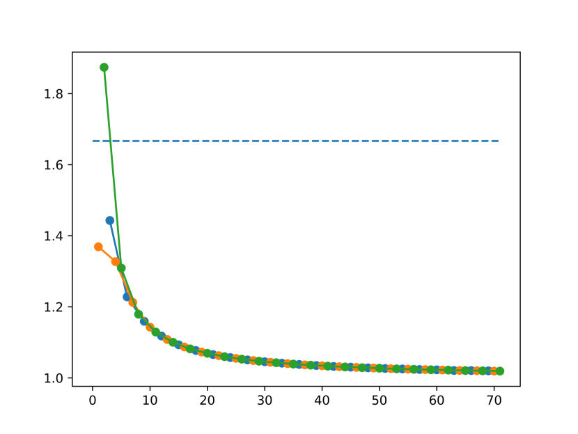
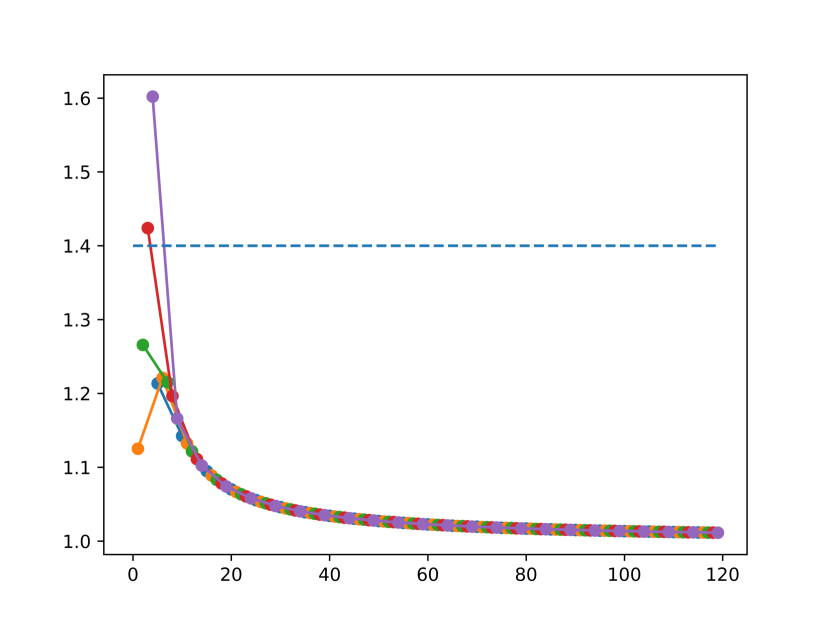
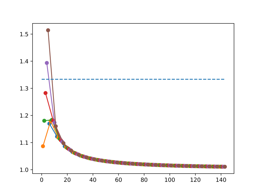
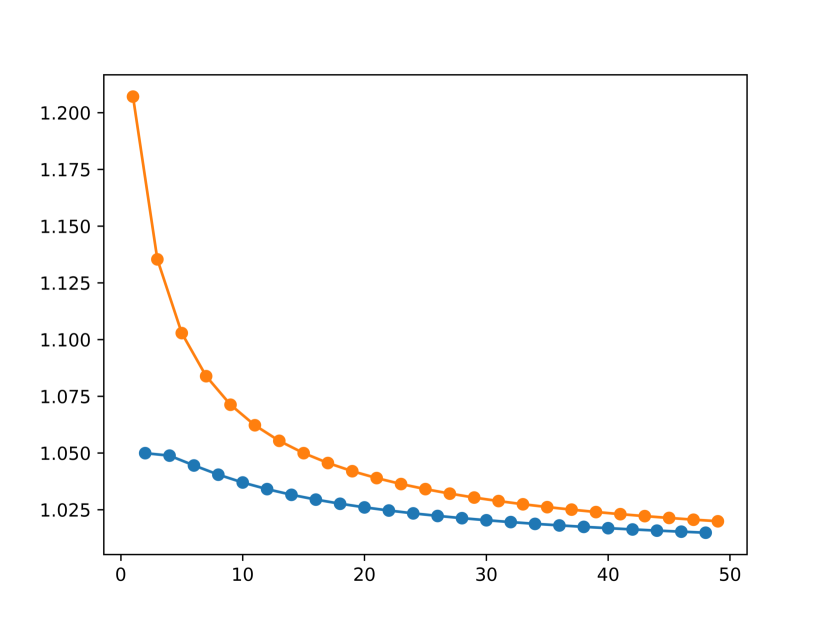
The corresponding Widom factors are illustrated in Table 1 and Figures 1(a)–1(d) and will be further discussed in Section 4.
| 1.3090 | 1.2784 | 1.2135 | 1.5142 | |
| 1.1427 | 1.1298 | 1.1424 | 1.1736 | |
| 1.0549 | 1.0497 | 1.0554 | 1.0632 | |
| 1.0271 | 1.0245 | 1.0272 | 1.0314 | |
| – | 1.0135 | 1.0150 | 1.0173 | |
| – | 1.0104 | 1.0112 | 1.0130 |
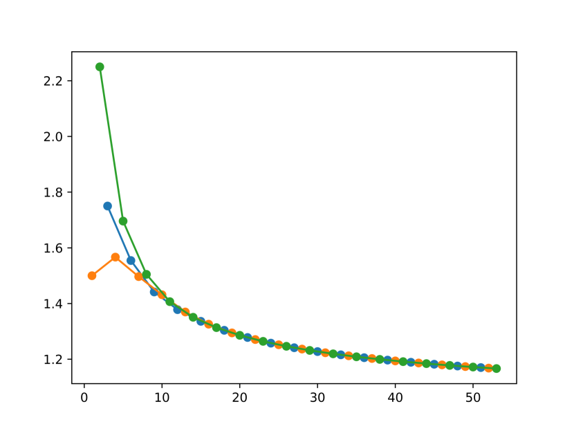
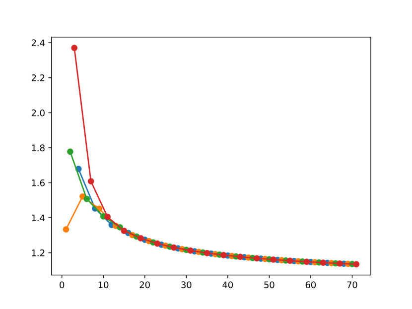
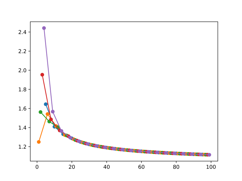
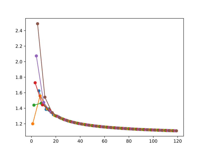
3.1.2 Hypocycloid
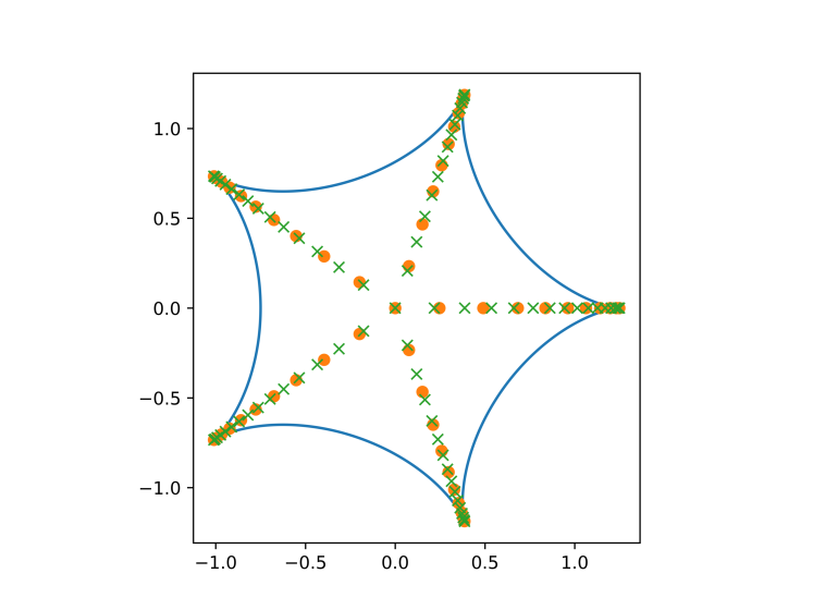
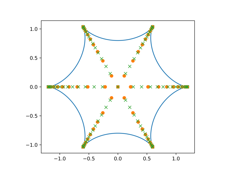
Examples of sets which are not quasi-circles are sets which contain outward pointing cusps on their boundary. With an “outward pointing cusp” we simply mean that the exterior angle at such a point is . For a pictorial representation the reader can consult Figures 5(g)-5(j) since examples of sets containing cusps are the -cusped hypocycloids. These are the Jordan curves defined via
| (19) |
It is easily seen that if is the external conformal map from the unbounded component of to satisfying as then
and hence for any .
The corresponding Faber polynomials have been studied in [23, 24]. Particular focus has been directed toward the corresponding zero distributions which are confined to straight lines.
Clearly the sets are invariant under rotations by and therefore Lemma 1 implies that
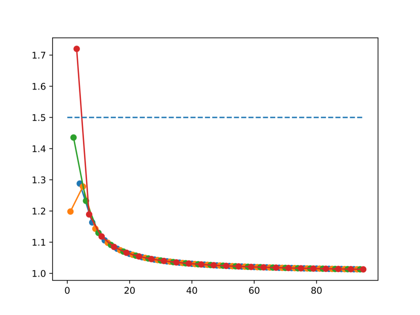
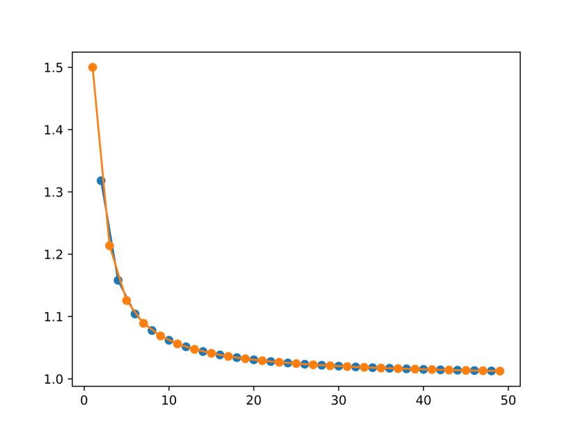
where is a monic polynomial with real coefficients. The corresponding Widom factors are illustrated in Table 2 and Figures 2(a)–2(d) and will be further discussed in section 4.
| 1.6959 | 1.5212 | 1.6445 | 2.48832 | |
| 1.4315 | 1.4078 | 1.4091 | 1.4744 | |
| 1.2518 | 1.2404 | 1.2493 | 1.2664 | |
| 1.1717 | 1.1626 | 1.1674 | 1.1759 | |
| – | 1.1113 | 1.1213 | 1.1269 |
3.1.3 Circular Lunes
As a final example of the computation of Widom factors we consider the case of circular lunes, see Figures 5(e) and 5(f). Given , we let
| (20) |
with vertices at and exterior angle . The structure of such sets heavily depend on the value of the parameter . If then the set is non-convex while if the set is convex. The extreme cases are and . We will consider two parameter values, namely and as they cover the cases of concavity and convexity. Irregardless of the parameter value of , the set is symmetric with respect to both axes. From Lemma 1 we conclude that
where is a monic polynomial of degree with real coefficients. The results of the computations using Tang’s algorithm are illustrated in Table 3 and Figures 3(a) and 3(b).
| 1.0404 | 1.0619 | |
| 1.0341 | 1.0244 | |
| 1.0212 | 1.0203 | |
| 1.0261 | 1.0174 | |
| 1.0213 | 1.0135 |
3.2 The Faber connection
Our initial interest in computing Chebyshev polynomials originated in studies of their zeros. One part of this study concerned Chebyshev polynomials on level curves corresponding to the exterior conformal map of a simply connected set . More precisely, if is the exterior conformal map we investigated Chebyshev polynomials on the level curves
and found that the corresponding zeros of seemed to converge for increasing . By simultaneously plotting the zeros of the Faber polynomials, the picture became quite clear. The zeros of , as increased, appeared to accumulate at the zeros of the corresponding Faber polynomials. We investigate this possible relation numerically for lemniscates, hypocycloids and circular lunes.
3.2.1 Lemniscates
For given parameters and , we define a family of compact lemniscatic sets via
| (21) |
A pictorial representation of such sets can be found in Figures 5(k) and 5(l). From (4) we gather that and since the polynomial saturates the lower bound in (3) we see that . For the remaining degrees we apply Lemma 1 to draw the conclusion that
| (22) |
where is a monic polynomial whose coefficients are all real. The parameter determines three separate regimes of sets.
-
•
If then is the closure of an analytic Jordan domain.
-
•
If , we write and in this case is connected however its interior is not.
-
•
If then consists of components.
Since , we see that for any and . The question is what the asymptotic behavior is for the remaining sequences of degrees. For it follows immediately from (8) that as since the boundary is an analytic Jordan curve. If then it is known that , see [51]. The remaining case, when , is handled by [5, Corollary 2] where it is shown that as .
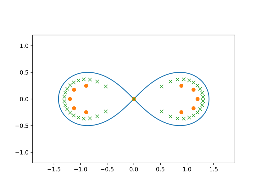
In the following discussion we limit ourselves to the case and write and . It should be stressed that analogous considerations are possible for any . The set is the classical Bernoulli lemniscate.
The conformal map taking to with is given by
where the branch is chosen such that at infinity. It follows from (7) that
and hence for any value of . We investigate if there is a possible relation between and as well.
It is possible to determine the Chebyshev polynomial of degree corresponding to explicitly by solving the system of equations
with . For a computation shows that the solution is given by
| (23) |
On the other hand, using the Taylor expansion of it is easy to see that
and hence we gather from (23) that uniformly on compact subsets of the complex plane. The question is whether this should be considered an anomaly or a potential link between Chebyshev polynomials and Faber polynomials. The natural procedure is of course to consider further examples. We do so numerically using Tang’s algorithm.
We define a norm on polynomials in the following way. If then is given by
| (24) |
Our aim with this is to display the difference
and illustrate that this appears to tend to with . Such a difference is illustrated in Figure 4(a).
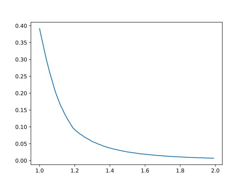
3.2.2 Hypocycloid
We continue the considerations concerning a possible relation between Faber polynomials and Chebyshev polynomials on level curves corresponding to conformal maps. We therefore return to the family of -cusped hypocycloids . The Faber polynomials can be computed using [24, Proposition 2.3].
For , we let
If denotes the external conformal map from the unbounded component of to with as then is the analytic Jordan curve where attains modulus . With the intention of considering the possibility that
as , we compute for . The graph is illustrated in Figure 4(b).
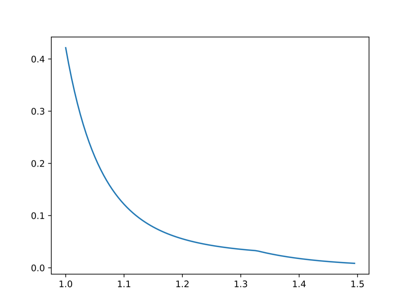
3.2.3 Circular Lunes
We end the considerations of comparing Chebyshev polynomials to Faber polynomials by considering the case of circular lunes. As an example we consider the case where . In this case the canonical external conformal map from the unbounded component of to the exterior of the closed unit disk has the simple form
We therefore find that
For , we let
The computed difference for is illustrated in Figure 4(c).

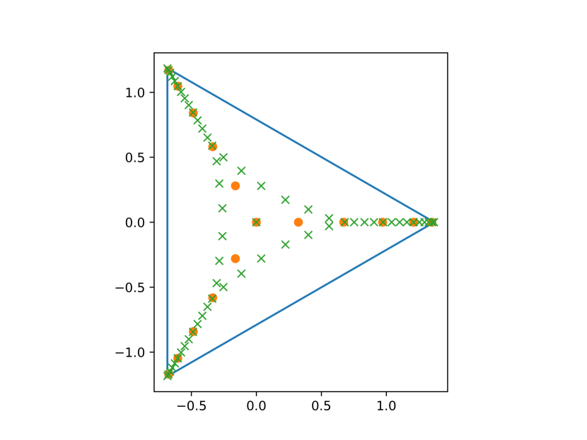
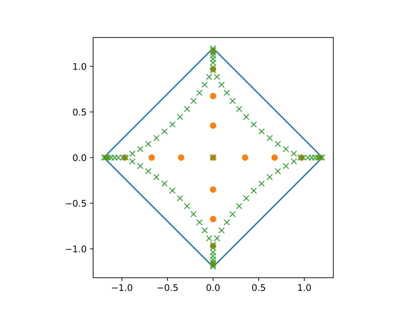
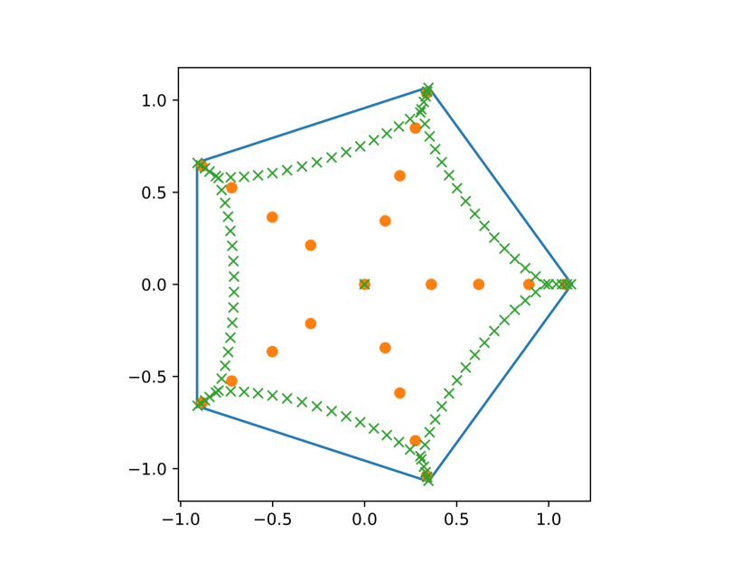
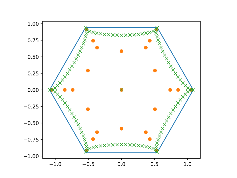
3.3 Zero distribution
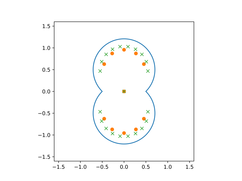
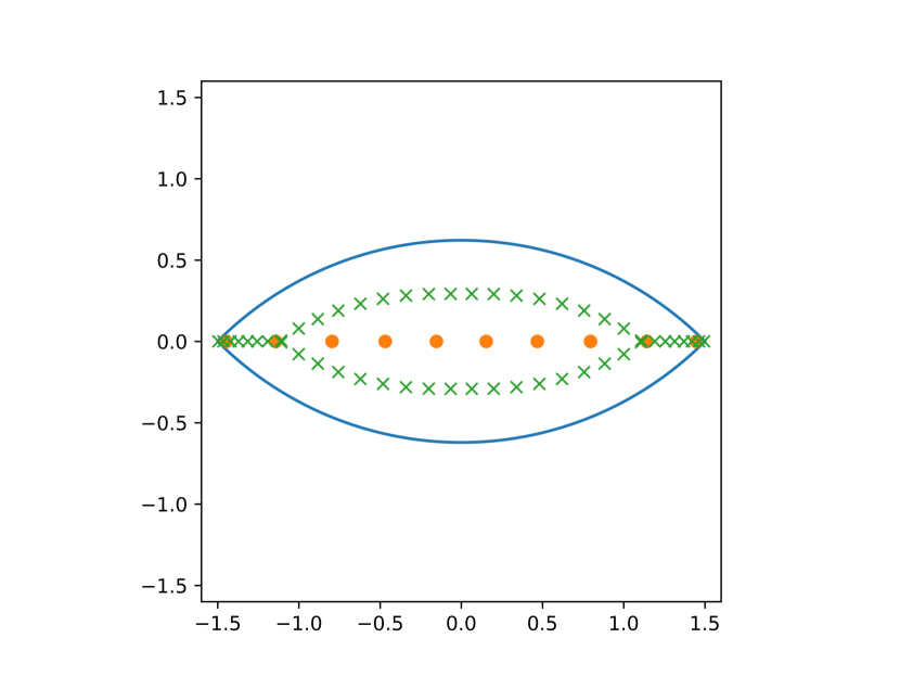
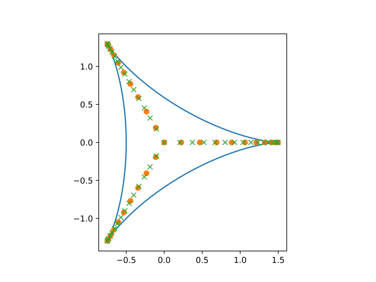
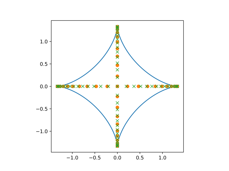
Our final computations concerns computing the zeros of for different compact sets . In Figures 5(a)-5(d) the zeros corresponding to , , and are computed. In Figures 5(e) and 5(f) the zeros of certain are illustrated for and . In Figures 5(g)–5(j) the zeros of certain are computed for different values of and . In Figures 5(k) and 5(l) the zeros corresponding to and are computed. To complement the plots of the zeros of we also plot the zeros of Chebyshev polynomials corresponding to two different families of lemniscates. In particular lemniscates of the form
The corresponding zero plots are given in Figures 5(m) and 5(n). We again stress the fact that the computations are approximative since we compute polynomials whose norms are close to .
4 Discussion
In Section 3 we saw several examples of computations of Chebyshev polynomials that we here wish to discuss further.
4.1 Widom factors
The Widom factors computed in Section 3 are computed to a high degree of accuracy. We believe that Tang’s algorithm can be very useful in getting suggested behavior regarding the Widom factors corresponding to a set. This method has previously been applied in [8] where a result on the limits of Widom factors – first conjectured using numerical experiments – was resolved theoretically. The conjecture whose validity we wish to argue for is the following.
Conjecture 1.
Let denote the closure of a Jordan domain with piecewise analytic boundary where none of the singularities of are cusp points. Then
4.1.1 Regular polygon
We begin by discussing the Widom factors computed for the regular polygons. As we previously remarked, it is known that these are bounded by due to the inherent convexity of the set but apart from this bound, not much is known. The plots in Figures 1(a)-1(d) clearly suggests that is monotonically decreasing in if and is an -gon. Furthermore, it seems to be the case that the Widom factors converge to . This is in accordance with Conjecture 1. The computations clearly suggests that there is differing behavior between Chebyshev polynomials and Faber polynomials corresponding to the regular -gon in terms of their supremum value. Indeed, by [31, Theorem II.2.1], we see that if is an -gon with corners at then
as for . In conclusion, we see that
We remark that the dotted lines visible in Figures 1(a)-1(d) represent the value . If we choose to believe that decrease monotonically for then as Figures 1(a)-1(d) illustrate, the norms of the Chebyshev polynomials are significantly smaller.
Based on these considerations, the Faber polynomials corresponding to the regular polygons presumably do not provide good enough estimates as trial polynomials to determine the limits of the Widom factors. In short, we believe that the sequence decreases monotonically if and that the limit is as .
One approach in proving that the limit value is is to analyze some well-suited family of trial polynomials whose normalized norms converge to . How to construct such a family is not immediately clear to us. Under the assumption that holds this would not constitute the only example where the Faber polynomials are ill-suited trial polynomials for determining the detailed behavior of . In the extreme case, an example of Clunie [13] further studied by Suetin [43, p. 179] and Gaier [17] illustrates the existence of a quasi-disk such that the quantity
is unbounded in along some sparse subsequence. In comparison [4, Theorem 1] shows that is still bounded in this case.
4.1.2 Hypocycloid
Recall that denotes the -cusped hypocycloid defined in (19). Since is piecewise analytic away from the cusp points which are outward pointing, [49, Theorem 2.1] can be applied to deduce that is bounded. The Faber polynomials again seem ill-suited in order draw conclusions concerning the precise behavior of the Widom factors in this case since it is shown in [24] that
for . Comparisons with Faber polynomials are therefore inconclusive as to whether
holds or not. The numerical experiments illustrated in Figures 2(a)-2(d) paint a richer picture. Again, it seems likely that the sequence decreases monotonically, suggesting that the sequence has a limit as . In comparison to the Widom factors of the regular -gons, the decay appears to be slower in this case. We find it reasonable to assume that that – if it exists – should be smaller than due to the monotonicity pattern and the values computed in Table 2. We find it difficult to say whether the correct conjecture is that the sequence converges to the theoretical minimal value of since the decay seems to be slow. For this reason we believe that “outward pointing cusps” should be excluded from Conjecture 1 since it is not clear even in the case of the -cusped hypocycloid if the associated Widom factors asymptotically saturates (3).
4.1.3 Circular lune
Recall that , defined in (20), denotes the circular lune with vertices at and exterior angle . Based on the plots in Figures 3(a) and 3(b) together with the computations in Table 3, it seems likely that the Widom factors corresponding to converges to . It is interesting to note that when the set is convex then the whole sequence appears to be monotonically decreasing, see Figure 3(b). On the other hand, if then two distinct monotonically decreasing subsequences of emerge based on the parity of the degrees. We believe that the sequence is monotonically decreasing to for fixed if . The case that is excluded for it is classical that for any value of . Also classical is the fact that . We believe that this example shows that for a nice enough bounding curve, it is not necessary that the set is convex for the sequence of Widom factors to converge to the theoretical minimal value. This also motivates our quite general formulation of Conjecture 1.
4.2 Motivating the Faber connection
The Chebyshev polynomials and Faber polynomials will both exhibit similar symmetric structure as the corresponding underlying set. To see this, one should compare Lemma 1 to [21, Theorem 2.2] or [22, Theorem 2.1]. This comparison is essentially encapsulated in the following simple lemma.
Lemma 2.
If is invariant under rotations of then both the Chebyshev polynomial and Faber polynomial of respective degrees are polynomials in multiplied by the factor for . In particular,
Proof.
Of course Lemma 2 has more to do with the rotational symmetry of a set than any other property. It does, however, give several easy examples where the two families of polynomials overlap.
If is a rectifiable Jordan curve and is the conformal map from the exterior of to of the form
then it can be shown that
for . If was a polynomial of degree then it would follow from (3) that it would coincide with the corresponding Chebyshev polynomial. We have already seen examples of this when studying lemniscates. Although this is rarely the case, we observe that will be an increasingly good candidate for obtaining relatively small maximum values on as . For a fixed degree , will be asymptotically minimal on in the sense that
We believe that this serves as motivation for why one could expect
as to hold in general. Based on the numerical data illustrated in Figure 4 this is clearly hinted upon for these specific domains. We therefore make the following conjecture.
Conjecture 2.
Let denote a connected compact set with simply connected complement and let denote the conformal map of the form
If then
We find the data presented in Figure 4 convincing in suggesting the validity of Conjecture 2 for these specific types of sets and remark that similar patterns have materialized for any other combination of degrees and sets that we have considered. In the general case it is clear that will be an analytic curve for and hence the regularity of the boundary of is perhaps of less importance since the Faber polynomials corresponding to are the same as the ones corresponding to . We stress again the fact that the algorithm outputs polynomials such that is small. This is not exactly the same as saying that is small with defined in (24). What is true, is that for a fixed , implies that . The computations remain consistent throughout. No matter how close we approximate the minimal norm, the behavior as suggested in Figure 4 remains.
4.3 Zero distributions
We recall that if is a polynomial then is the probability measure defined in Section 1 via the formula
where are the zeros of counting multiplicity. Also, given a compact set we use to denote the equilibrium measure on .
It is shown in [40] that the zeros corresponding to the closure of a Jordan domain stay away from the boundary precisely when the bounding curve is analytic. As such we see that in all of our examples, except for the cases of lemniscates with analytic boundary, the zeros should approach some part of the boundary. From [11, Theorem 1.1] we gather that every “corner point” on the respective sets , and should attract zeros. This also appears to be the case, albeit, slowly for .
Predicting the behavior of zeros of extremal polynomials based on plots has proven hazardous in the past. In particular, we refer to the reader to [38] where five conjectures concerning limiting zero distributions are made very plausible using numerical plots only to be proven to be wrong using theoretical results. However, if one chooses to believe that Conjecture 2 is true then this alludes to the possibility that potential weak-star limits of and are related. In the cases where we boldly propose conjectures regarding weak-star convergence of we emphasize that the corresponding weak-star limits of the counting measures are known to have this very behavior.
4.3.1 Regular polygons
We adopt the notation to denote the regular polygon with sides. As is suggested by Figures 5(a)-5(d), the zeros of for low degrees appear to lie on the diagonal lines between the vertices and the origin. However, by increasing the degree it seems clear that the zeros approach the boundary. In [38] the case of Faber polynomials on are discussed. Here the authors specify that for small degrees the zeros of appear to distribute along the diagonals however they also note that as a consequence of [29, Theorem 1.5] at least a subsequence of converges in the weak-star sense to which is supported on the boundary. The zeros of certain are illustrated in [22] and appear to behave very similar to the ones for computed here. We therefore believe that the zeros should approach the boundary in the sense that (11) should hold for every compact set in the interior. This would of course also imply that
as .
4.3.2 Circular lune
Recall the definition of from (20). Based on the plot in Figure 5(e) it appears as most of the zeros approach the boundary in the case when and that (11) should hold for any compact set contained in the interior. This is in fact a known result and follows from [39, Theorem 2.1]. Indeed, from there we gather that as for any . In this sense the computed polynomials serves to confirm the predicted behaviour from theoretical results. For any value of it follows from [29, Theorem 1.5] that along some subsequence. Again, motivated by the belief that the conjectured similarities between Chebyshev polynomials and Faber polynomials persists for together with the strong resemblance between the plots of zeros for Faber polynomials in [22] with the corresponding zeros of computed here, we suspect that
for any value of . Note that and hence has all its zeros at the origin.
Based on the examples of the regular polygons and circular lunes together with our belief that Conjecture 2 is valid we conjecture the following result which is a partial reformulation of [29, Theorem 1.5] to the setting of Chebyshev polynomials. We define a singularity point of a piecewise analytic curve as a point where the derivative of the arc-length parametrization of the curve has limits from either sides but form an angle to each other.
Conjecture 3.
Let denote the closure of a Jordan domain with piecewise analytic boundary such that has a singularity other than an outward cusp. Then there is a subsequence such that
4.3.3 Hypocycloid
The reason that an outward cusp is excluded in Conjecture 3 is that the result does not hold in the Faber setting if the bounding curve has an outward cusp as is shown in [24]. Indeed, exactly as is the case for Faber polynomials, we believe that the example of an hypocycloid provides an example where the zeros of do not approach all of the boundary. It is clearly suggested by Figures 5(g)-5(j) that the support of is confined to the diagonals between the cusps and the origin for all values of computed. This is in accordance with the behavior exhibited by and we believe that an analogous result as [24, Theorem 3.1] is true in this case.
Conjecture 4.
The zeros of for are confined to the set
| (25) |
Again, if we choose to believe Conjecture 2 then this together with Conjecture 25 would imply that the zeros of would move along the straight diagonals as increases and approach the corresponding zeros of the Faber polynomials, this is something we find reasonable to believe.
On the other hand, we note that numerical simulations indicate that the zeros of the corresponding Bergman polynomials corresponding to and its interior, all lie on the straight lines in (25) for small degrees. However it follows from [38, Theorem 2.1] that at least a subsequence of the Bergman polynomials have zero counting measures converging weak-star to .
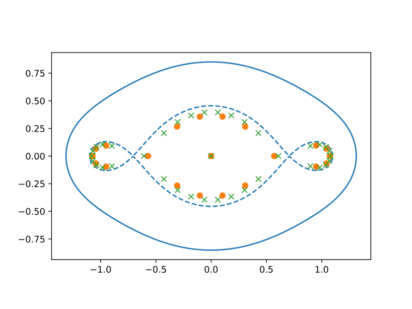
4.3.4 Lemniscate
Recall that , and that . Based on Figure 5(k) it seems reasonable to assume that
| (26) |
for any compact set contained in . It actually appears to be the case that all the zeros approach the boundary. The main theorem in [40], which states that zeros of Chebyshev polynomials corresponding to an analytic Jordan curve stay away from the boundary is not applicable in this case because does not have a connected interior. If (26) could be established, a consequence of this would be that converges in the weak-star sense to the equilibrium measure on . It should be noted in this regard that by changing the variable to it follows that
where is the monic minimizer of the expression
Corresponding to each weight of the form for there is a minimizing weighted Chebyshev polynomial which we denote with , see [5]. In the particular case where it is shown in [5, Theorem 3] that converges weak-star to equilibrium measure on . This implies that an analogous result as (26) is valid for compact subsets of . There is no reason to believe that such a result should exclusively hold for the parameter value of and we therefore suspect that
Note that for any and hence very different zero behavior would be exhibited for the different subsequences if the conjecture is true. This is however the case for the Faber polynomials. From a result in [50], it follows that
Furthermore, it is shown there that all the zeros of lie on or inside .
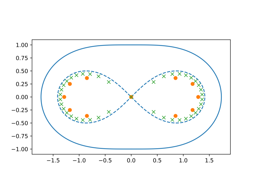
We turn our attention to the outer lemniscates with . Surprisingly, based on Figure 5(l) it seems like the zeros of all lie strictly inside except for the single zero at . Although the main Theorem in [40] implies that the zeros asymptotically stay away from there is no results hinting toward the fact the zeros seem to cluster on . If one believes Conjecture 2 so that as then it is reasonable to assume that the zeros of lie on or inside for all values of and since the zeros of have this very behavior.
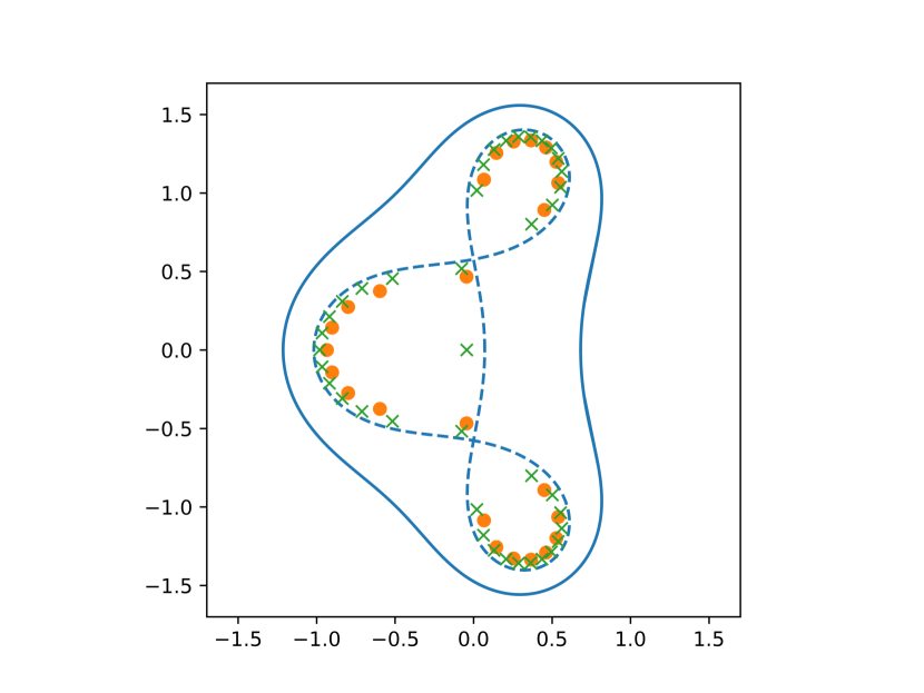
Analogous results seem to hold true with replaced by for any value of as the corresponding numerical simulations indicate the same pattern. Generalizations of Ullmans result concerning the asymptotic zero distribution of the Faber polynomials on can be found in [21]. We further believe that a general version of the above result can be formulated for any connected lemniscate. To understand this perspective we introduce the notion of a critical value of a polynomial. This is a number where is such that . The polynomial has one critical value, namely which is attained at the origin. This implies that the curve will contain a critical point of resulting in the fact that the curve forms a crossing with itself at the origin. In general, if is a critical value of a polynomial then will contain a crossing point.
If we consider the polynomial then has two critical values, namely and . Upon inspection of Figure 5(m) it becomes apparent that the zeros of the Chebyshev polynomials on the curve seem to approach the critical curve which correspond to the lemniscate where the largest critical value is attained (in modulus). Equivalently, this curve is characterized by being the curve with smallest value of which is connected.
A similar pattern emerges for the lemniscates of the form with , see Figure 5(n). For the polynomial the critical point is and the corresponding critical value is . Since we see that the critical lemniscate corresponds to . Again, this critical lemniscate seems to attract the zeros of the Chebyshev polynomials corresponding to larger values of . We believe that this can be formulated as a general result as we have observed this very behavior for all lemniscates that we have considered.
Conjecture 5.
Let be a polynomial of degree with largest critical value in terms of absolute value given by . For any let
then for a fixed
as .
Based on Figures 5(m) and 5(n) this seems to be the case. Observe that (5) implies that where is the leading coefficient of in which case the zero counting measure is constant.
It could be further speculated what happens in the general case for level curves of conformal maps. Assume that is a connected compact set with simply connected complement and is the conformal map of the form as . Again, introducing the set then the bounding curve of is analytic for . From [40] we know that the zeros of asymptotically stay away from the boundary, in the sense that there exists a neighborhood of the boundary where is zero free for large . The question is if something similar as in the case of lemniscates happens in this situation. Do the zeros asymptotically approach ? This is true for the corresponding Faber polynomials and therefore the validity of Conjecture 2 could hint at this being true for the corresponding Chebyshev polynomials.
4.4 Concluding remarks
With this article, we hope to exemplify the usefulness of Tang’s generalization of the Remez algorithm to the study of Chebyshev polynomials. Our research into the matters commenced by considering the zeros of the Chebyshev polynomials corresponding to the Bernoulli lemniscate
Based on the fact that it was suggested in [10] that the odd Chebyshev polynomials which apart from having a zero at the origin should behave similarly. Explicitly it is written on [10, p. 215] that “…we suspect (but cannot prove) that for large all the other zeros of lie in small neighborhoods of and that the above is also the limit through odd ’s.” Here . We initially set out to show this. Since we did not progress in this regard we started considering numerical methods to compute the Chebyshev polynomials with the intent of better understanding how the zeros approached . Using Tang’s algorithm we could compute the Chebyshev polynomials corresponding to and the result surprised us. The zeros seemed to behave opposite to our conjecture and approached the bounding curve rather than the two points . The use of the algorithm therefore showed us that the hypothesis we initially had believed was probably incorrect and that our conjecture should be modified. We made partial progress in proving Conjecture 3 in [5] by showing that a related problem satisfied the conjectured behavior. However, we are still lacking a complete proof of this.
With the algorithm at hand we set out to study Chebyshev polynomials corresponding to a wide variety of sets whose asymptotic behavior remain unknown. We believe that making use of the algorithm is a good way of getting predictions on the behavior of Chebyshev polynomials. The results in [5] and [8] are based on conjectures formulated using initial numerical experiments. Some rather surprising results have also been suggested to us by numerical experiments along the way. In particular, the relation between Faber polynomials and Chebyshev polynomials specified in Conjecture 2 does not seem to have been given any attention in the literature in the past although the fact that they coincide for certain sets is known.
In short, we believe that use of Tang’s algorithm in the study of Chebyshev polynomials may prove useful in the future when formulating conjectures on their asymptotic behavior.
Appendix A Tang’s algorithm
We recall that Tang’s algorithm seeks a linear functional
| (27) |
conditioned to satisfy , , , and for every . The goal with applying the algorithm is to obtain coefficients such that
is minimal.
The linear nature of the maximizing linear functional suggests that it is beneficial to change the perspective to linear algebra. We use the notation from [45, 46, 27, 16] and define the matrix
| (28) |
together with the vector
| (29) |
It then follows from (13) that
| (30) |
and the constraints (14) and (15) become embedded in the equation
| (31) |
Parameters satisfying (31) are called admisible if additionally is invertible. If , , is a best approximation and , are corresponding admissible parameters such that then
| (32) |
and therefore if is invertible we can recover the extremal coefficients from and . We assume, as in [45, 46, 16] that (which is no restriction) since we can always parametrize using . To emphasize that we are working on we let .
For an implementation of the algorithm in Python, see [37].
Acknowledgement
The author is grateful to Frank Wikström and Jacob Stordal Christiansen, both at Lund University. The former for providing excellent advice on the presentation of the numerical experiments in this manuscript and the latter for helpful discussions on the material presented herein.
References
- [1] F. G. Abdullayev, V. V. Savchuk, and T. Tunç. Exact estimates for Faber polynomials and for norm of Faber operator. Complex Var. Elliptic Equ., 65:293–305, 2020.
- [2] N. I. Achieser. Theory of approximation. Frederick Ungar publishing co. New York, 1956.
- [3] V. Andrievskii and H.-P. Blatt. Discrepancy of Signed Measures and Polynomial Approximation. Springer New York, 2001.
- [4] V. Andrievskii and F. Nazarov. On the Totik–Widom property for a quasidisk. Constr. Approx., 50:497–505, 2019.
- [5] A. Bergman and O. Rubin. Chebyshev polynomials corresponding to a vanishing weight. J. Approx. Theory (to appear), 2024.
- [6] P. L. Chebyshev. Théorie des mécanismes connus sous le nom de parallélogrammes. Mém. des sav. étr. prés. à l’Acad. de. St. Pétersb., 7:539–568, 1854.
- [7] E. W. Cheney. Introduction to approximation theory. McGraw-Hill book company, 1966.
- [8] J. S. Christiansen, B. Eichinger, and O. Rubin. Extremal polynomials and polynomial preimages. arXiv, 2312.12992, 2023.
- [9] J. S. Christiansen, B. Simon, and M. Zinchenko. Asymptotics of Chebyshev polynomials, I. subsets of . Invent. Math., 208:217–245, 2017.
- [10] J. S. Christiansen, B. Simon, and M. Zinchenko. Asymptotics of Chebyshev polynomials, III. sets saturating Szegő, Schiefermayr, and Totik–Widom bounds. Oper. Theory Adv. Appl., 276:231–246, 2020.
- [11] J. S. Christiansen, B. Simon, and M. Zinchenko. Asymptotics of Chebyshev polynomials, IV. Comments on the complex case. JAMA, 141:207–223, 2020.
- [12] J. S. Christiansen, B. Simon, and M. Zinchenko. Asymptotics of Chebyshev polynomials, V. Residual polynomials. Ramanujan J., 61:251–278, 2023.
- [13] J. Clunie. On schlicht functions. Ann. Math., 69:511–519, 1959.
- [14] G. Faber. Über Tschebyscheffsche polynome. J. Reine Angew. Math., 150:79–106, 1919.
- [15] V. Faber, J. Liesen, and P. Tichý. On chebyshev polynomials of matrices. SIAM J. Matrix Anal. Appl., 31:2205–2221, 2010.
- [16] B. Fischer and J. Modersitzki. An algorithm for complex linear approximation based on semi-infinite programming. Numer. Algor., 5:287–297, 1993.
- [17] D. Gaier. The Faber operator and its boundedness. J. Approx. Theory, 101:265–277, 1999.
- [18] A. Goncharov and B. Hatinoğlu. Widom factors. Potential Anal., 42:671–680, 2015.
- [19] A. Greenbaum and L. N. Trefethen. GMRES/CR and Arnoldi/Lanczos as matrix approximation problems. SIAM J. Sci. Comput., 15:359–368, 1994.
- [20] U. Grothkopf and G. Opfer. Complex Chebyshev polynomials on circular sectors with degree six or less. Math. Comput., 39:599–615, 1982.
- [21] M. He. The Faber polynomials for -fold symmetric domains. J. Comput. Appl. Math., 54:313–324, 1994.
- [22] M. He. Numerical results on the zeros of Faber polynomials for -fold symmetric domains. In Exploiting symmetry in applied and numerical analysis, Lectures in Appl. Math., pages 229–240. Amer. Math. Soc., 1994.
- [23] M. He. Explicit representations of Faber polynomials for -cusped hypocycloids. J. Approx. Theory, 87:137–147, 1996.
- [24] M. He and E. B. Saff. The zeros of Faber polynomials for an -cusped hypocycloid. J. Approx. Theory, 78:410–432, 1994.
- [25] A. Iske. Approximation theory and algorithms for data analysis. Springer–Verlag GmbH, Heidelberg, 2018.
- [26] S. O. Kamo and P. A. Borodin. Chebyshev polynomials for Julia sets. Moscow Univ. Math. Bull., 49:44–45, 1994.
- [27] M. Z. Komodromos, S. F. Russell, and P. T. P. Tang. Design of fir filters with complex desired frequency response using a generalized remez algorithm. IEEE Trans. Circuits Syst. II, 42:274–278, 1995.
- [28] T. Kövari and Ch. Pommerenke. On Faber polynomials and Faber expansions. Math. Z., 99:193–206, 1967.
- [29] A. Kuijlaars and E. B. Saff. Asymptotic distribution of the zeros of Faber polynomials. Math. Proc. Camb. Phil. Soc., 118:437–447, 1995.
- [30] P. D. Lax. Functional analysis. John Wiley & Sons, Inc., 2002.
- [31] E. Miña Díaz. Asymptotics for Faber polynomials and polynomials orhogonal over regions in the complex plane. PhD thesis, Vanderbilt University, 2006.
- [32] G. Opfer. An algorithm for the construction of best approximations based on Kolmogorov’s criterion. J. Approx. Theory, 23:299–317, 1978.
- [33] T. Ransford. Potential theory in the complex plane. Cambridge university press, 1995.
- [34] E. Remez. Sur la détermination des polynômes d’approximation de degré donnée. Comm. Soc. Math. Kharkov, 10:41–63, 1934.
- [35] E. Remez. Sur un procédé convergent d’approximations successives pour déterminer les polynômes d’approximation. Compt. Rend. Acad. Sc., 198:2063–2065, 1934.
- [36] T. J. Rivlin. Chebyshev polynomials: from approximation theory to algebra and number theory. John Wiley & sons, Inc., New York, 1990.
- [37] O. Rubin. Remez–Tang algorithm. https://github.com/olguvirubin/remez-tang-algorithm, 2024.
- [38] E. B. Saff and N. S. Stylianopoulos. Asymptotics for polynomial zeros: Beware of predictions from plots. Comput. Methods Funct. Theory., 8:385–407, 2008.
- [39] E. B. Saff and N. S. Stylianopoulos. On the zeros of asymptotically extremal polynomial sequences in the plane. J. Approx. Theory, 191:118–127, 2015.
- [40] E. B. Saff and V. Totik. Zeros of Chebyshev polynomials associated with a compact set in the plane. SIAM J. Math. Anal., 21:799–802, 1990.
- [41] V. I. Smirnov and N. A. Lebedev. Functions of a complex variable: constructive theory. The M.I.T. press, Massachusetts Institute of Technology, Cambridge, Massachusetts, 1968.
- [42] P. K. Suetin. Polynomials orthogonal over a region and bieberbach polynomials. In Proceedings of the Steklov institute of mathematics. American mathematical society, Providence, Rhode Island, 1974.
- [43] P. .K Suetin. Series of Faber polynomials. Gordon and Breach science publishers, Amsterdam, The Netherlands, 1998.
- [44] G. Szegő. Bemerkungen zu einer Arbeit von Herrn M. Fekete: Über die Verteilung der Wurzeln bei gewissen algebraischen Gleichungen mit ganzzahligen Koeffizienten. Math. Z., 21:203–208, 1924.
- [45] P. T. P. Tang. Chebyshev approximation on the complex plane. PhD thesis, University of California at Berkeley, 1987.
- [46] P. T. P. Tang. A fast algorithm for linear complex Chebyshev approximation. Math. Comp., 51:721–739, 1988.
- [47] J.-P. Thiran and C. Detaille. Chebyshev polynomials on circular arcs and in the complex plane. In Progress in Approximation Theory, pages 771–786. Academic Press, Boston, MA, 1991.
- [48] K-.C. Toh and L. N. Trefethen. The Chebyshev polynomial of a matrix. SIAM J. Matrix Anal. Appl., 20:400–419, 1998.
- [49] V. Totik and T. Varga. Chebyshev and fast decreasing polynomials. Proc. Lond. Math. Soc., 110:1057–1098, 2015.
- [50] J. L. Ullman. Studies in Faber polynomials. I. Trans. Am. Math. Soc., 94:515–528, 1960.
- [51] H. Widom. Extremal polynomials associated with a system of curves in the complex plane. Adv. in Math., 3:127–232, 1969.