TIT/HEP-701 May 2024 Inductive calculation of superconformal indices
based on giant graviton expansion

We investigate a simple-sum giant graviton expansion of the superconformal indices of ${\cal N}=2$ superconformal field theories realized on D3-branes probing $7$-brane backgrounds with constant axio-dilation field. The expansion is of self-dual type, and imposes strong constraints on the indices. By using the constraints we determine first few terms in the superconformal indices for arbitrary rank $N$.

1 Introduction

AdS/CFT correspondence [1, 2, 3] is usually regarded as a duality between a $d$-dimensional boundary field theory and a $d+1$ dimensional bulk theory including gravity. This duality have been extensively studied in the large $N$ limit, and a lot of evidences have been found. For example, in the correspondence between the ${\cal N}=4$ $U(N)$ SYM and the type IIB string theory in $AdS_{5}\times S^{5}$, the superconformal index [4, 5], which is the quantity we focus on in this paper, was calculated on the both sides of the correspondence in the large $N$ limit, and the agreement was confirmed [5].

The correspondence is believed to hold even for finite $N$. Formulas giving the finite $N$ superconformal index on the AdS side have been proposed [6, 7, 8], and are called giant graviton expansions. In the expansions, the finite $N$ corrections are included as the contributions of giant gravitons [9, 10] wrapped around cycles in the internal manifolds. They are calculated as the indices of field theories on giant gravitons. Therefore, a giant graviton expansion can be regarded as a set of relations between two classes of field theories: boundary field theories with different ranks and theories realized on brane systems labeled by wrapping numbers.

We consider superconformal theories $T_{N}$ with rank $N=1,2,3,\ldots$, and their superconformal indices $I_{N}$. The general form of a giant graviton expansion is

$$\frac{I_{N}}{I_{\infty}}=\sum_{\vec{m}}x_{1}^{m_{1}N}\cdots x_{k}^{m_{k}N}F_{m_{1},\ldots,m_{k}}.$$ (1)

where $\sum_{\vec{m}}$ is the summation over $k$ non-negative wrapping numbers $m_{1},\ldots,m_{k}$. $k$ depends on the theories; $k=3$ for ${\cal N}=4$ $U(N)$ SYM and orbifold theories [6, 11], and for more general quiver gauge theories realized on D3-branes probing toric Calabi-Yau three-folds, $k$ is the number of the corners of the toric diagram [12]. Other examples have been also studied [13, 14, 15].

It was found in [8] that (1) reduces to a simple-sum giant graviton expansion for ${\cal N}=4$ $U(N)$ SYM by adopting an appropriate expansion scheme. Namely, if we treat $F_{m_{1},\ldots,m_{k}}$ as a power series with respect to an appropriate fugacity $\mathfrak{t}$, $F_{m_{1},\cdots,m_{k}}$ is non-vanishing only when $m_{2}=\cdots=m_{k}=0$ and then the multiple-sum expansion (1) reduces to a simple-sum over $m:=m_{1}$. See also [16, 17] for the mechanism of the reduction to the simple-sum. The non-trivial contributions $F_{m,0,\ldots,0}$ are essentially the superconformal indices of theories $T_{m}^{\prime}$ realized on the worldvolume of the stack of $m$ giant gravitons. More precisely, $F_{m,0,\ldots,0}$ is obtained from the index $I^{\prime}_{m}$ of $T_{m}^{\prime}$ by a simple variable change of fugacities [6, 8], which is schematically given by $F_{m,0,\ldots,0}(\mathfrak{t},s,u_{i})=I_{m}^{\prime}(\mathfrak{t},s^{-1},\widetilde{u}_{i})$. As the result, the giant graviton expansion is given by

$$\frac{I_{N}(\mathfrak{t},s,u_{i})}{I_{\infty}(\mathfrak{t},s,u_{i})}=\sum_{m=0}^{\infty}s^{mN}I^{\prime}_{m}(\mathfrak{t},s^{-1},\widetilde{u}_{i}),$$ (2)

where $\widetilde{u}_{i}$ is a certain permutation of $u_{i}$. With this relation, we can calculate the indices $I_{N}$ with arbitrary $N$ from the indices of another class of theories $I^{\prime}_{m}$ with different ranks $m$.

In general, $T_{N}$ and $T^{\prime}_{N}$ may be different theories. For example, the indices of M2-brane theories (ABJM theories) and M5-brane theories ($(2,0)$ theories of type $A$) are related by the expansion in the form (2) [16]. More examples of such pairs of four-dimensional field theories related by (2) are studied in [17]. Such relations are useful when we know the indices on one side of the relation.

In this work, in contrast, we consider the self-dual situation: the case that the theories $T_{N}$ and $T^{\prime}_{N}$ appearing on the two sides of the giant graviton expansion are the same. In this case the giant graviton expansion is given by

$$\frac{I_{N}(\mathfrak{t},s,u_{i})}{I_{\infty}(\mathfrak{t},s,u_{i})}=\sum_{m=0}^{\infty}s^{mN}I_{m}(\mathfrak{t},s^{-1},\widetilde{u}_{i}).$$ (3)

This is similar to (2), but the same indices $I_{N}$ (with different arguments) appear on the two sides of the relation. This is the case for the ${\cal N}=4$ SYM with $U(N)$ gauge group [8]. Another example is the ${\cal N}=2$ theory realized on D3-branes probing an O7-plane background [17], which we denote by $D_{4}[N]$ below. In this work, we study a class of ${\cal N}=2$ superconformal field theories including the above two as special cases; ${\cal N}=2$ superconformal field theories realized on D3-branes probing $7$-brane backgrounds with constant axio-dilaton field.

(3) is expected to hold for an arbitrary $N$, and imposes very strong constraints on the set of functions $I_{N}$, and it is likely that we can determine complete indices form a small piece of information obtained by some analysis independent of the giant graviton expansion. The purpose of this work is to discuss to what extent (3) constrains the indices and explicitly determine first few terms of them starting from a partial information.

2 Strategy

If we know the holographic dual description of $T_{N}$, we can calculate the large $N$ index $I_{\infty}(\mathfrak{t},s,u_{i})$ by the mode analysis of massless fields on the AdS side. So, let us treat $I_{\infty}$ as a known function. Then, (3) gives infinitely many linear relations among $I_{N}(\mathfrak{t},s,u_{i})$ and $I_{m}(\mathfrak{t},s^{-1},\widetilde{u}_{i})$.

As we mentioned in Introduction, we treat the index as a power series

$$I_{N}(\mathfrak{t},s,u_{i})=\sum_{k=0}^{\infty}\mathfrak{t}^{k}f_{N,k}(s,\widetilde{u}_{i})$$ (4)

in an appropriately chosen fugacity $\mathfrak{t}$. As we will see later, $\mathfrak{t}$ is a fugacity associated with a Cartan generator of a non-Abelian symmetry, and the charge is quantized to be integer. This guarantees that the power series in (4) includes only integral powers of $\mathfrak{t}$. (This is not the case for $s$. The functions $f_{N,k}(s,\widetilde{u}_{i})$ include fractional powers of $s$.) The form of the expansion (simple-sum/multiple-sum) depends on the expansion scheme, and the simple-sum expansion works only when we first expand functions with respect to the specific fugacity $\mathfrak{t}$ as in (4).

A nice property of the expansion (4) is that a truncation at an arbitrary $k=k_{*}$ gives a closed set of relations among $f_{N,k}$ with $k\leq k_{*}$, and we can discuss inductive determination of $f_{N,k}$ in the order $k=0,1,2,\ldots$.

Let us first consider the truncation at $k_{*}=0$, which gives the following relation among $f_{N,0}$:

$$\frac{f_{N,0}(s,u_{i})}{f_{\infty,0}(s,u_{i})}=\sum_{m=0}^{\infty}s^{mN}f_{m,0}(s^{-1},\widetilde{u}_{i}).$$ (5)

The presence of $s^{-1}$ on the right hand side makes the analysis complicated. Naive use of series expansion in $s$ does not work because the expansion coefficients of $f_{N,0}(s)$ and those of $f_{N,0}(s^{-1})$ are not directly related, and we need to analytically continue the functions around $s=0$ to those around $s=\infty$.

Fortunately, we know the analytic forms of these functions. As we will discuss below, the functions are nothing but the Coulomb branch index. The theory $T_{N}$ we discuss is defined as the theory on a stack of $N$ D3-branes and $N$ independent Coulomb branch operators exist. The Coulomb branch index depends only on $s$, and we denote $f_{N,0}(s,u_{i})$ simply by $f_{N}(s)$ in the following. They are given by

$$f_{N}(s)=\prod_{i=1}^{N}\frac{1}{1-s^{i}},$$ (6)

and we can easily confirm that these functions satisfy (5) [8].

Next, let us discuss $f_{N,1}$. It is convenient to define $g_{N,k}$ by

$$g_{N,k}(s,u_{i})=\frac{f_{N,k}(s,u_{i})}{f_{N}(s)}.$$ (7)

We first focus on $g_{N,1}$, and we denote them by $g_{N}$. By picking up $\mathfrak{t}^{1}$ terms from (3) we obtain

$$g_{N}(s,u_{i})-g_{\infty}(s,u_{i})=\frac{f_{\infty}(s)}{f_{N}(s)}\sum_{m=0}^{\infty}s^{mN}f_{m}(s^{-1})g_{m}(s^{-1},\widetilde{u}_{i}).$$ (8)

By assumption, $f_{N}$ and $g_{\infty}$ are known functions and this equation gives linear constraints on unknown functions $g_{N}$.

A nice property of $g_{N}$ ($N<\infty$) is that they are fractional polynomials of $s$. By “a fractional polynomial of $s$” we mean a function of $s$ in the form

$$\sum_{j}c_{j}s^{r_{j}}$$ (9)

with a finite number of terms. Unlike an ordinary polynomial, the exponents $r_{j}$ may not be non-negative integers. They may be fractional and negative. Because the number of terms is finite, the exponents $r_{j}$ are within a finite range depending on $N$. This is not the case for $f_{N,1}$. The $s$-expansion of $f_{N,1}$ includes infinitely many terms. This is due to the presence of the Coulomb branch operators. Let ${\cal O}$ be a BPS operator contributing to $f_{N,1}$. Then, a product of ${\cal O}$ and Coulomb branch operators also contributes to the same function $f_{N,1}$, and this makes $f_{N,1}$ an infinite series of $s$. In the definition (7) of $g_{N,k}$ the contribution from the Coulomb branch operators is removed by the division by $f_{N}$.

To express the range of the exponents we use the notation

$$s^{n^{L}(N)}\leq g_{N}(s,u_{i})\leq s^{n^{H}(N)}.$$ (10)

This means that the exponents $r_{j}$ appearing in $g_{N}(s,u_{i})$ are in the range $n^{L}(N)\leq r_{j}\leq n^{H}(N)$. If $g_{N}(s,u_{i})$ is a fractional polynomial bounded by (10), $g_{N}(s^{-1},\widetilde{u}_{i})$ is also a fractional polynomial bounded by

$$s^{-n^{H}(N)}\leq g_{N}(s^{-1},\widetilde{u}_{i})\leq s^{-n^{L}(N)}.$$ (11)

We do not need analytic continuation to relate $s$-expansions of $g_{N}(s,u_{i})$ and $g_{N}(s^{-1},\widetilde{u}_{i})$.

Let us consider inductive determination of $g_{N}$. Namely, we suppose that we have obtained $g_{N}$ for $N\leq N_{*}-1$ with a fixed rank $N_{*}$, and discuss whether we can determine $g_{N_{*}}$ by the relation (8). We can use (8) in two different ways.

1. If we set $N=N_{*}$ in (8) the left hand side includes $g_{N_{*}}(s,u_{i})$. We obtain the relation

   $$g_{N_{*}}(s,u_{i})=(\mbox{known})+\frac{f_{\infty}(s)}{f_{N_{*}}(s)}\sum_{m=N_{*}}^{\infty}s^{mN_{*}}f_{m}(s^{-1})g_{m}(s^{-1},\widetilde{u}_{i}),$$ (12)

   where “$(\mbox{known})$” includes known functions only. Although the right hand side includes unknown functions $g_{m}(s^{-1},\widetilde{u}_{i})$ with $m\geq N_{*}$, if they give only higher order terms in $s$, then we may be able to extract information of low order terms in $g_{N_{*}}(s,u_{i})$.

2. If we set $N$ in (8) to be a value smaller than $N_{*}$, then the left hand side is a known function, and the summand with $m=N_{*}$ on the right hand side includes $g_{N_{*}}(s^{-1},\widetilde{u}_{i})$. We can rewrite (8) as

   $$g_{N_{*}}(s^{-1},\widetilde{u}_{i})=(\mbox{known})-\sum_{m=N_{*}+1}^{\infty}\frac{s^{mN}f_{m}(s^{-1})}{s^{N_{*}N}f_{N_{*}}(s^{-1})}g_{m}(s^{-1},\widetilde{u}_{i}).$$ (13)

   With this relation it may be possible to extract information of low order terms in $g_{N_{*}}(s^{-1},\widetilde{u}_{i})$, or equivalently, high order terms in $g_{N_{*}}(s,u_{i})$.

Because these two approaches give information of different parts of $g_{N_{*}}(s,u_{i})$, it may be possible to completely determine $g_{N_{*}}(s,u_{i})$ by combining these two.

Let $\mathfrak{o}_{1}(N_{*})$ be the order of the second term in (12). If we use the bound (11) we obtain

$$\mathfrak{o}_{1}(N_{*}):=\min_{m\geq N_{*}}\left(mN_{*}+\frac{m(m+1)}{2}-n^{H}(m)\right).$$ (14)

(The second term in the parentheses comes from $f_{N}(s^{-1})=(-1)^{N}s^{\frac{N(N+1)}{2}}f_{N}(s)$.) To determine the minimum value (14) we need to know $n^{H}(m)$. Although we do not have precise expression for $n^{H}(N)$ at present, we will later see that numerical analysis suggests that $n^{H}(N)$ grows as a linear function of $N$. Then, the minimum $\mathfrak{o}_{1}(N_{*})$ always exists and we can determine $s^{n<\mathfrak{o}_{1}(N_{*})}$ terms in $g_{N_{*}}(s,u_{i})$ with the relation (12) .

The leading order of the unknown part of (13) for each $m$ is

$$(m-N_{*})N+\frac{m(m+1)}{2}-\frac{N_{*}(N_{*}+1)}{2}-n^{H}(m).$$ (15)

$N$ is assumed to be smaller than $N_{*}$. We want the order to be as large as possible. To maximize the order we set $N=N_{*}-1$, and then the order of the unknown part of (13), which we denote by $\mathfrak{o}_{2}(N_{*})$, becomes

$$\mathfrak{o}_{2}(N_{*}):=\min_{m\geq N_{*}+1}\left((m-N_{*})\frac{m+3N_{*}-1}{2}-n^{H}(m)\right).$$ (16)

Again, under the assumption of linear growth of $n^{H}(m)$, the minimum always exists. We can determine $s^{n<\mathfrak{o}_{2}(N_{*})}$ terms in $g_{N_{*}}(s^{-1},\widetilde{u}_{i})$, or, equivalently, $s^{n>-\mathfrak{o}_{2}(N_{*})}$ terms in $g_{N_{*}}(s,u_{i})$.

Let us combine the two results. The relation (12) determines $s^{n<\mathfrak{o}_{1}(N_{*})}$ terms in $g_{N_{*}}(s,u_{i})$, and the relation (13) determines $s^{n>-\mathfrak{o}_{2}(N_{*})}$ terms in $g_{N_{*}}(s,u_{i})$. Therefore, we can determine $g_{N_{*}}(s,u_{i})$ completely by combining these two relations if

$$0<\mathfrak{o}_{1}(N_{*})+\mathfrak{o}_{2}(N_{*}).$$ (17)

Under the assumption of linear growth of $n^{H}(N)$, this always hold for sufficiently large $N_{*}$. Namely, there exists $N_{\rm crit}$ such that (17) holds for arbitrary $N_{*}\geq N_{\rm crit}$. The value of $N_{\rm crit}$ depends on the explicit form of $n^{H}(N)$. If $N_{\rm crit}$ is not so large, we can determine $g_{N}$ for all $N$ by directly calculating $g_{N}$ for $N<N_{\rm crit}$ and apply the procedure explained above.

The same strategy can be applied to the higher order terms in the expansion (5). To avoid the analysis becomes too abstract, we first apply the above analysis for $g_{N}(s,u_{i})$ to concrete examples and then we will proceed to the analysis of the higher order terms.

3 ${\cal N}=2$ superconformal field theories

Brane realization

We consider the ${\cal N}=2$ superconformal theory realized on a stack of $N$ D3-branes probing a $7$-brane background of the form

$$\mathbb{R}^{1,3}\times\mathbb{R}^{4}_{H}\times{\cal C}.$$ (18)

The D3 branes extend along $\mathbb{R}^{1,3}$, the four-dimensional Minkowski space. They probe the six-dimensional transverse space $\mathbb{R}^{4}_{H}\times{\cal C}$, where $\mathbb{R}^{4}_{H}=\mathbb{C}_{x}\times\mathbb{C}_{y}$ is the flat four-dimensional space and ${\cal C}$ is the complex one-dimensional cone with the deficit angle $2\pi(1-\Delta^{-1})$. If $N=1$ the transverse space ${\cal C}$ and $\mathbb{R}_{H}^{4}$ are identified with the Coulomb branch and the Higgs branch of the moduli space, respectively. $\Delta$ is the scale dimension of the Coulomb branch operator with the smallest dimension. The tip of ${\cal C}$ is singular and gives the $7$-brane worldvolume in the ten-dimensional spacetime.

Let $X$, $Y$, and $Z$ be complex coordinates of $\mathbb{C}_{x}$, $\mathbb{C}_{y}$, and $\cal C$, respectively. Due to the deficit angle, $Z$ is restricted by

$$0\leq\arg Z\leq\frac{2\pi}{\Delta}$$ (19)

and boundary points of the sector are identified by

$$Z=r\quad\sim\quad Z=re^{\frac{2\pi i}{\Delta}}\quad(r\in\mathbb{R}_{\geq 0}).$$ (20)

There exist seven non-trivial $\cal C$ specified by the values of $\Delta$. We use the symbols $G=H_{0}$, $H_{1}$, $H_{2}$, $D_{4}$, $E_{6}$, $E_{7}$, and $E_{8}$ to specify one of them. See Table 1.

Table 1:

$G$	$H_{0}$	$H_{1}$	$H_{2}$	$D_{4}$	$E_{6}$	$E_{7}$	$E_{8}$
$\Delta$	$\frac{6}{5}$	$\frac{4}{3}$	$\frac{3}{2}$	$2$	$3$	$4$	$6$
symmetry	-	$su(2)$	$su(3)$	$so(8)$	$e_{6}$	$e_{7}$	$e_{8}$

We also use $G$ to specify the gauge symmetry realized on the $7$-brane. We denote the theory on $N$ D3-branes by $G[N]$.

Each of these theories includes a free hypermultiplet corresponding to the center-of-mass motion of D3-branes along $\mathbb{R}_{H}^{4}$. Although these non-interacting degrees of freedom are often excluded from the definition of the theory, we includes their contribution to the superconformal index in the following analysis. The rank $1$ theories $H_{0}[1]$, $H_{1}[1]$, and $H_{2}[1]$ with the free hypermultiplet excluded are the Argyres-Douglas theories [18, 19] often called $(A_{1},A_{2})$, $(A_{1},A_{3})$, and $(A_{1},D_{4})$, respectively. $E_{n}[1]$ ($n=6,7,8$) with the free hypermultiplet excluded are called Minahan-Nemeschansky theories [20, 21].

In addition to seven non-trivial cases, we regard ${\cal N}=4$ $U(N)$ SYM as the special case with $\Delta=1$.

Superconformal index

The global symmetry of $G[N]$ is

$$su(2,2|2)\times su(2)_{F}\times G,$$ (21)

where $su(2,2|2)$ is the ${\cal N}=2$ superconformal algebra with Cartan generators $H$, $J$, $\overline{J}$, $R$, and $r$. $H$ is the Hamiltonian, $J$ and $\overline{J}$ are the left and the right spins, and $R$ and $r$ are $su(2)_{R}$ and $u(1)_{r}$ charges. We normalize these generators so that the supercharges carry the following quantum numbers

$$Q:(H,J,\overline{J},R,r) =(+\tfrac{1}{2},\pm\tfrac{1}{2},0,\pm\tfrac{1}{2},-\tfrac{1}{2}),$$

$$\overline{Q}:(H,J,\overline{J},R,r) =(+\tfrac{1}{2},0,\pm\tfrac{1}{2},\pm\tfrac{1}{2},+\tfrac{1}{2}).$$ (22)

$su(2)_{F}\times G$ is the flavor symmetry, and we use $F$ and $T_{i}$ ($i=1,\ldots,\mathop{\rm rank}\nolimits G$) for their Cartan generators. We normalize $F$ to be half integer. $su(2)_{F}$ and $G$ are realized as the isometry of $\mathbb{R}_{H}^{4}$ and the gauge symmetry on the 7-brane, respectively. For the ${\cal N}=4$ SYM $su(2,2|2)\times su(2)_{F}$ is enhanced to $psu(2,2|4)$, and $G$ is trivial.

Let $\overline{\cal Q}$ be the component of $\overline{Q}$ with the quantum numbers

$$\overline{\cal Q}:(H,J,\overline{J},R,r)=(+\tfrac{1}{2},0,-\tfrac{1}{2},+\tfrac{1}{2},+\tfrac{1}{2}).$$ (23)

The superconformal index respecting the supercharge $\overline{\cal Q}$ is defined by

$$I=\mathop{\rm tr}\nolimits\left[(-1)^{F}t^{2\overline{J}+2R}u^{2J}v^{2F}z^{\overline{J}+r}\prod_{i=1}^{\mathop{\rm rank}\nolimits G}a_{i}^{T_{i}}\right],$$ (24)

where $t$, $u$, $v$, $z$, and $a_{i}$ are independent fugacities.

It is also convenient to introduce generators $J_{1}$, $J_{2}$, $R_{x}$, $R_{y}$, and $R_{z}$ by

$$J_{1}=\overline{J}+J,\quad J_{2}=\overline{J}-J,\quad R_{x}=R+F,\quad R_{y}=R-F,\quad R_{z}=r.$$ (25)

$R_{x}$, $R_{y}$, and $R_{z}$ rotate $\mathbb{C}_{x}$, $\mathbb{C}_{y}$, and ${\cal C}$, respectively. Corresponding to the new set of generators we define

$$q=tz^{1/2}u,\quad p=tz^{1/2}u^{-1},\quad x=tv,\quad y=tv^{-1}.$$ (26)

Four fugacities defined in (26) and $z$ are not independent but constrained by $qp=xyz$. With these variables, the index (24) is rewritten as

$$I=\mathop{\rm tr}\nolimits\left[(-1)^{F}q^{J_{1}}p^{J_{2}}x^{R_{x}}y^{R_{y}}z^{R_{z}}\prod_{i=1}^{\mathop{\rm rank}\nolimits G}a_{i}^{T_{i}}\right].$$ (27)

Only states saturating the BPS bound

$$0\leq\{\overline{\cal Q},\overline{\cal Q}^{\dagger}\} =H-2\overline{J}-2R-r$$

$$=H-J_{1}-J_{2}-R_{x}-R_{y}-R_{z}$$ (28)

contribute to the index.

Holographic dual

The holographic dual geometry is $AdS_{5}\times S^{5}_{\Delta}$, where $S^{5}_{\Delta}$ is a five-dimensional sphere with a conical defect along a large $S^{3}$ [22, 23]. $S^{5}_{\Delta}$ is explicitly defined by

$$|X|^{2}+|Y|^{2}+|Z|^{2}=1^{2},$$ (29)

with the coordinates introduced above.

Under the assumption that giant graviton contributions localize at the $U(1)_{R_{x}}\times U(1)_{R_{y}}\times U(1)_{R_{z}}$ fixed points in the D3-brane configuration space, we expect that giants wrapped on the following three three-cycles in $S_{\Delta}^{5}$ contribute to the index,

$$X=0,\quad Y=0,\quad Z=0,$$ (30)

and the corresponding giant graviton expansion is [15]

$$\frac{I_{N}}{I_{\infty}}=\sum_{m_{x},m_{y},m_{z}=0}^{\infty}x^{m_{x}N}y^{m_{y}N}z^{\Delta m_{z}N}F_{m_{x},m_{y},m_{z}},$$ (31)

where $F_{m_{x},m_{y},m_{z}}$ are the indices of the theories realized on the giant gravitons with wrapping numbers $m_{x}$, $m_{y}$, and $m_{z}$. This triple-sum expansion were studied in [15] with a focus on the contributions from $(m_{x},m_{y},m_{z})=(1,0,0)$ and $(0,1,0)$.

Self-dual giant graviton expansion

We are interested in a self-dual giant graviton expansion. This requires the theory on giant gravitons $T_{N}^{\prime}$ are the same as the original theory $T_{N}$. For this to be the case the giant gravitons must wrap on the singular locus $Z=0$. This is the case if we choose expansion variable $\mathfrak{t}=t$. (We will later slightly change the definition of $\mathfrak{t}$. See (36).)

With this choice of the expansion variable, two cycles $X=0$ and $Y=0$ decouple [16, 17]. We obtain the giant graviton expansion of the form

$$\frac{I_{N}}{I_{\infty}}=\sum_{m=0}^{\infty}z^{m\Delta_{G}}F_{0,0,m},$$ (32)

where $F_{0,0,m}$ is essentially the same as $I_{m}$. The variable change transforming $F_{0,0,m}$ into $I_{m}$ is related to an outer automorphism of the unbroken symmetry on the worldvolume of giant gravitons [6]. The symmetry preserved by giant gravitons wrapped around the cycle $Z=0$ is

$$u(2|2)\times su(2)_{J}\times su(2)_{F}\times G,$$ (33)

where $u(2|2)=su(2|2)\rtimes u(1)_{r}$ is the algebra generated by $\overline{Q}$ and $\overline{Q}^{\dagger}$. (More precisely, $\overline{Q}$ and $\overline{Q}^{\dagger}$ generates $su(2|2)$, and the extension by its outer automorphism $u(1)_{r}$ generated by $r=R_{z}$ gives $u(2|2)$.) The outer automorphism of the preserved symmetry algebra (33)

$$\overline{J}\leftrightarrow R,\quad J\leftrightarrow F,\quad R_{z}\rightarrow-R_{z},\quad H-R_{z}\rightarrow H-R_{z}$$ (34)

relates the theory on the boundary and the theory on the cycle $Z=0$. This is consistent with the definition of the superconformal index (27), and the definition is invariant under (34) if we do the following variable change $\sigma_{z}$ at the same time.

$$\sigma_{z}(q,p,x,y,z)=(x,y,q,p,z^{-1}),\quad\sigma_{z}(t,z,y,u)=(tz^{1/2},z^{-1},u,y)$$ (35)

To match the form of the variable change with the one used in previous sections, we define the following variables.

$$\mathfrak{t} =tz^{\frac{1}{4}},$$

$$s =z^{\Delta},$$

$$u_{i} =(u,v,a_{i}),$$

$$\widetilde{u}_{i} =(v,u,a_{i}).$$ (36)

Then, $\sigma_{z}$ acts on these variables as follows.

$$\sigma_{z}(\mathfrak{t},s,u_{i})=(\mathfrak{t},s^{-1},\widetilde{u}_{i}),$$ (37)

and (31) is rewritten into the form (3).

Schur index

The Schur index [24] is defined by tuning the fugacities so that another supercharge ${\cal Q}$ in $Q$ is respected. Without loosing generality we can choose ${\cal Q}$ with the quantum numbers

$${\cal Q}:(H,J,\overline{J},R,r)=(+\tfrac{1}{2},-\tfrac{1}{2},0,+\tfrac{1}{2},-\tfrac{1}{2}).$$ (38)

To respect this supercharge we need to set $p=z$.

The Schur index is in general more tractable than the general superconformal index, and it is often possible to obtain analytic expression for them [25, 26, 27, 28]. It would be nice if we could discuss self-dual giant graviton expansion for Schur index. Unfortunately, it is not possible. The BPS bound associated with ${\cal Q}$ is

$$0\leq\{{\cal Q},{\cal Q}^{\dagger}\} =H-2J-2R+r$$

$$=H-J_{1}+J_{2}-R_{x}-R_{y}+R_{z}.$$ (39)

Only states saturating two bounds (28) and (39) at the same time contribute to the Schur index, but giant gravitons wrapped on $Z=0$ does not saturate (39). Furthermore, the Schur limit $p=z$ is inconsistent with the variable change (35). For these reasons we will not discuss the Schur limit in this work.

Large $N$ limit

The relation between the operator spectrum of $G[\infty]$ and Kaluza-Klein modes in the dual geometry was investigated in [22, 23], and the corresponding index was calculated in [15].

Let $i_{\infty}$ be the letter index in the holographic description. The large $N$ index $I_{\infty}$ is given by $I_{\infty}=\mathop{\rm Pexp}\nolimits i_{\infty}$. $i_{\infty}$ is the sum of two contributions [15]:

$$i_{\infty}=f^{\rm(sugra)}+f^{(7)}\chi_{\rm adj}^{G}.$$ (40)

$f^{\rm(sugra)}$ is the letter index of the supergravity multiplet in the ten-dimensional bulk

$$f^{\rm(sugra)} =\frac{[(x+y)-xy+xy(q+p)]-[(x^{\prime}+y^{\prime})-x^{\prime}y^{\prime}+x^{\prime}y^{\prime}(q^{\prime}+p^{\prime})]}{(1-q)(1-p)(1-x)(1-y)}$$

$$+\frac{s}{1-s}\frac{(1-q^{\prime})(1-p^{\prime})(1-x^{\prime})(1-y^{\prime})}{(1-q)(1-p)(1-x)(1-y)},$$ (41)

where we defined

$$q^{\prime}=\frac{q}{z},\quad p^{\prime}=\frac{p}{z},\quad x^{\prime}=zx,\quad y^{\prime}=zy.$$ (42)

The second term in (40) is the contribution from the vector multiplet on the seven-brane. $\chi_{\rm adj}^{G}$ is the adjoint character of the symmetry $G$ and $f^{(7)}$ is the letter index of the $u(1)$ vector multiplet on the eight-dimensional worldvolume of the seven-brane

$$f^{(7)}=\frac{xy-pq}{(1-q)(1-p)(1-x)(1-y)}.$$ (43)

We can write the letter index for $\Delta=1$ (corresponding to the ${\cal N}=4$ $U(N)$ SYM) in the form (40) by formally setting $\chi_{\rm adj}^{G}=-2$.

4 Observation

The arguments in Section 2 is based on the assumption of linear growth of $n^{H}(N)$. To confirm this and to obtain more explicit form of $n^{H}(N)$, let us look at some examples obtained by numerical calculations. We use two-dimensional plots to express the structure of the series expansion of indices. See Figure 1.

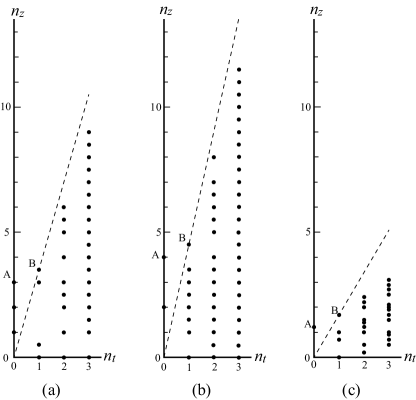
Figure 1: 2d plots of $\mathop{\rm Plog}\nolimits I$. (a) ${\cal N}=4$ $U(3)$ SYM (b) ${\cal N}=2$ $Sp(2)$ SQCD ($D_{4}[2]$) (c) $H_{0}[1]$. $A$ is the Coulomb branch operator with the largest dimension and $B$ is its conformal descendant determining the envelope line.

We showed the plethystic logarithm of the index, $\mathop{\rm Plog}\nolimits I$, as a two-dimensional plot for three theories: ${\cal N}=4$ $U(3)$ SYM ($\Delta=1$, $N=3$), $D_{4}[2]$ ($\Delta=2$, $N=2$), and $H_{0}[1]$ ($\Delta=\frac{6}{5}$, $N=1$). The horizontal and vertical axes are the exponents of $t$ and $z$, respectively. Namely, a term $f(u,v)t^{n_{t}}z^{n_{z}}$ is shown as a dot at coordinates $(n_{t},n_{z})$.

Due to the BPS bounds all dots are in the first quadrant (including its boundary) in the $n_{t}$-$n_{z}$ plane, and $n_{t}$ is quantized to be integer. There are $N$ dots at even intervals on the vertical axis. They correspond to the Coulomb branch operators $\varphi_{k}$ $(k=1,\ldots,N)$ with dimensions $k\Delta$.

Except for those on the vertical axis, there are no dots above the envelope line passing through the origin and the dot at $(1,N\Delta+\frac{1}{2})$, which is labeled by $B$ in Figure 1. The dot $B$ corresponds to conformal descendants $\partial\varphi_{N}$ of the Coulomb branch operator $\varphi_{N}$ with the largest dimension. This means that the exponents $n_{t}$ and $n_{z}$ satisfy

$$0\leq n_{z}\leq n_{t}\left(N\Delta+\frac{1}{2}\right).$$ (44)

We rewrite the index as the function of $\mathfrak{t}$, $s$, and $u_{i}$, and express it as $\mathfrak{t}$ series

$$I_{N}(\mathfrak{t},s,u_{i})=f_{N}(s)\left[1+\sum_{k=1}^{\infty}\mathfrak{t}^{k}g_{N,k}(s,u_{i})\right].$$ (45)

The bound (44) means

$$s^{n^{L}_{k}(N)}\leq g_{N,k}(s,u_{i})\leq s^{n^{H}_{k}(N)}.$$ (46)

with

$$n^{L}_{k}=-\frac{k}{4\Delta},\quad n^{H}_{k}=k\left(N+\frac{1}{4\Delta}\right).$$ (47)

Although we have no rigorous proof of (47), let us take it as a working hypothesis.

5 $\mathfrak{t}^{1}$ terms

Let us continue the analysis of $g_{N}(=g_{N,1})$ in Section 2 by using the upper bound $n^{H}(N)=n^{H}_{1}(N)$:

$$n^{H}(N)=N+\frac{1}{4\Delta}.$$ (48)

By substituting this into (14) and (16) we obtain

$$\mathfrak{o}_{1}(N_{*}) =\frac{3}{2}N_{*}^{2}-\frac{1}{2}N_{*}-\frac{1}{4\Delta},$$ (49)

$$\mathfrak{o}_{2}(N_{*}) =N_{*}-1-\frac{1}{4\Delta},$$ (50)

for positive $N_{*}$, and the condition (17) becomes

$$\frac{3}{2}N_{*}^{2}+\frac{1}{2}N_{*}-1-\frac{1}{2\Delta}>0.$$ (51)

This condition is satisfied for all positive $N_{*}$. Namely, if we know the index for $N=0$ (and $N=\infty$), we can uniquely determine $g_{N}$ for all $N$ by requiring the self-dual giant graviton expansion holds. The theory with $N=0$ is the trivial theory with $I_{0}=1$, and $g_{0}=0$.

We can give an analytic solution satisfying the relation (8). Let us take the ansatz

$$g_{N}(s,u_{i})=(1-s^{N})g_{\infty}(s,u_{i}).$$ (52)

This is consistent with the large $N$ limit, and correctly reproduces $g_{0}=0$. Although we can obtain $g_{\infty}$ by expanding (40), let us discuss without using the explicit form for the present. By substituting (52) into (8) the right hand side of (8) becomes

$$(\mbox{r.h.s}) =\frac{f_{\infty}(s)}{f_{N}(s)}\sum_{m=1}^{\infty}s^{mN}f_{m-1}(s^{-1})g_{\infty}(s^{-1},\widetilde{u}_{i})$$

$$=s^{N}\frac{f_{\infty}(s)}{f_{N}(s)}\sum_{m=0}^{\infty}s^{mN}f_{m}(s^{-1})g_{\infty}(s^{-1},\widetilde{u}_{i})$$

$$=s^{N}g_{\infty}(s^{-1},\widetilde{u}_{i})$$ (53)

At the second equality $m$ is replaced by $m+1$ and at the third equality (5) is used. The left hand side of (8) becomes $-s^{N}g_{\infty}(s,u_{i})$, and the relation (8) reduces to

$$g_{\infty}(s^{-1},\widetilde{u}_{i})=-g_{\infty}(s,u_{i}).$$ (54)

The consistency requires $g_{\infty}(s,u_{i})$ satisfy the non-trivial relation (54).

In fact, this is the case. As is pointed out in [17], the large $N$ letter indices $i_{\infty}$ satisfies the interesting relation

$$i_{\infty}(\mathfrak{t},s,u_{i})+i_{\infty}(\mathfrak{t},s^{-1},\widetilde{u}_{i})=-1,$$ (55)

and the $\mathfrak{t}^{1}$ terms in (55) give (54).

(54) can be also confirmed with the explicit form of $g_{\infty}(s,u_{i})$ obtained by expanding (40);

$$g_{\infty}=\frac{1-z}{1-s}z^{-\frac{1}{4}}(\chi_{1}^{v}-sz^{-\frac{1}{2}}\chi_{1}^{u}),$$ (56)

where $\chi_{n}^{u}$ and $\chi_{n}^{v}$ are $su(2)_{J}$ and $su(2)_{F}$ characters, respectively;

$$\chi_{n}^{u}=\frac{u^{n+1}-u^{-n-1}}{u-u^{-1}},\quad\chi_{n}^{v}=\frac{v^{n+1}-v^{-n-1}}{v-v^{-1}}.$$ (57)

By substituting (56) into (52) we obtain $g_{N}$;

$$g_{N}(s,u_{i}) =\frac{(1-z)(1-s^{N})}{1-s}z^{-\frac{1}{4}}[\chi_{1}^{v}-sz^{-\frac{1}{2}}\chi_{1}^{u}].$$ (58)

Because the prescription in Section 2 unambiguously determine $g_{N}$, (52) is the unique solution to (8). Indeed, we can confirm that (58) is consistent with the known results for $N=1$. The superconformal indices of the rank $1$ theories, $H_{0}[1]$ [29], $H_{1}[1]$ [30], $H_{2}[1]$ [31], and $D_{4}[1]$ are known and given by the unified form

$$I_{1} =\mathop{\rm Pexp}\nolimits\bigg{[}s+(1-z)(-sz^{-\frac{1}{2}}\chi_{1}^{u}+\chi_{1}^{v})t$$

$$+(1-z)(sz^{-1}-z-s^{2}z^{-1}-s\chi_{2}^{u}+z^{\frac{1}{2}}\chi_{1}^{u}\chi_{1}^{v}+(1-s)\chi_{\rm adj}^{G})t^{2}+{\cal O}(t^{3})\bigg{]}.$$ (59)

up to $t^{2}$ terms (See Appendix). The indices of $E_{6}[1]$ [32] and $E_{7}[1]$ [33] are also known, and (59) is consistent with the terms explicitly shown in the references. (59) also gives the index of the ${\cal N}=4$ $U(1)$ super Maxwell theory by setting $\Delta=1$ and $\chi_{\rm adj}^{G}=-2$. (58) agrees with $g_{1}$ extracted from (59).

6 $\mathfrak{t}^{k\geq 2}$ terms

Let us proceed to higher order terms in the expansion (4). We discuss whether we can determine $g_{N_{*},k_{*}}$ for fixed $N_{*}$ and $k_{*}$ when we know $g_{N,k}$ for $k\leq k_{*}-1$ and $g_{N,k_{*}}$ for $N\leq N_{*}-1$. Basic strategy is the same as before. We use the giant graviton expansion in two ways.

First, we extract $\mathfrak{t}^{k_{*}}$ terms from the giant graviton expansion of $I_{N_{*}}$. We obtain

$$g_{N_{*},k_{*}}(s,u_{i}) =(\mbox{known})+\frac{f_{\infty}(s)}{f_{N_{*}}(s)}\sum_{m=N_{*}}^{\infty}s^{mN_{*}}f_{m}(s^{-1})g_{m,k_{*}}(s^{-1},\widetilde{u}_{i}).$$ (60)

This is essentially the same as (12), and we obtain the following order of the unknown part.

$$\mathfrak{o}_{1,k_{*}}(N):=\min_{m\geq N_{*}}\left(mN_{*}+\frac{m(m+1)}{2}-n^{H}_{k_{*}}(m)\right).$$ (61)

Only difference from (14) is that $n^{H}(m)$ is replaced by $n^{H}_{k_{*}}(m)$. By using $n^{H}_{k_{*}}$ in (47) we obtain

$$\mathfrak{o}_{1,k_{*}}(N)=\frac{3}{2}N_{*}^{2}+\frac{1}{2}N_{*}-k_{*}\left(N_{*}+\frac{k_{*}}{4\Delta}\right).$$ (62)

Another relation is obtained from ${\cal O}(\mathfrak{t}^{k_{*}})$ terms in the giant graviton expansion of $I_{N}$ with $N<N_{*}$. We obtain the relation corresponding to (13)

$$g_{N_{*},k_{*}}(s^{-1},\widetilde{u}_{i})=(\mbox{known})-\sum_{m=N_{*}+1}^{\infty}\frac{s^{mN}f_{m}(s^{-1})}{s^{N_{*}N}f_{N_{*}}(s^{-1})}g_{m,k_{*}}(s^{-1},\widetilde{u}_{i}).$$ (63)

To make the order of the unknown part as large as possible we set $N=N_{*}-1$ and obtain

$$\mathfrak{o}_{2,k_{*}}(N) =\min_{m\geq N_{*}+1}\left((m-N_{*})N+\frac{m(m+1)}{2}-\frac{N_{*}(N_{*}+1)}{2}-n^{H}_{k}(m)\right)$$

$$=2N_{*}-k\left(N_{*}+1+\frac{1}{4\Delta}\right).$$ (64)

Therefore, the condition that we can completely determine $g_{N,k}$ is

$$0<\mathfrak{o}_{1,k_{*}}(N)+\mathfrak{o}_{2,k_{*}}(N)=\frac{3}{2}N_{*}^{2}+\frac{5}{2}N_{*}-k_{*}\left(2N_{*}+1+\frac{1}{2\Delta}\right).$$ (65)

Again, this condition is satisfied for sufficiently large $N_{*}$.

For $k_{*}=2$, this is satisfied for $N_{*}\geq N_{\rm crit}=2$ (for $\Delta>1$) or for $N_{*}\geq N_{\rm crit}=3$ (for $\Delta=1$). Let us consider $\Delta>1$ case first. Because $N_{\rm crit}=2$, it is guaranteed that if we use $g_{\infty,2}$ extracted from (40), $g_{1,2}$ extracted from (59), and $g_{0,2}=0$ as input data, the self-dual giant graviton expansion uniquely determines $g_{N,2}$ for arbitrary $N$. We find the following solution.

$$g_{N,2}(s,u_{i}) =\frac{(1-z)(1-s^{N})}{1-s}z^{-\frac{1}{2}}(sz^{-1}(1-s^{N})-z+(z^{\frac{1}{2}}-(s-s^{N})z^{-\frac{1}{2}})\chi_{1}^{u}\chi_{1}^{v}$$

$$-s\chi_{2}^{u}+(1-s^{N-1})\chi_{2}^{v}+(1-s)\chi_{\rm adj}^{G})+\frac{1}{2}(g_{N,1}(s^{2},u_{i}^{2})+g_{N,1}^{2}(s,u_{i})).$$ (66)

By combining $g_{N,1}(=g_{N})$ in (58) and $g_{N,2}$ in (66), we obtain the index

$$I_{N} =\mathop{\rm Pexp}\nolimits\bigg{[}\frac{s(1-s^{N})}{1-s}+\frac{(1-z)(1-s^{N})}{1-s}(-sz^{-\frac{1}{2}}\chi_{1}^{u}+\chi_{1}^{v})t$$

$$+\frac{(1-z)(1-s^{N})}{1-s}(sz^{-1}(1-s^{N})-z+(z^{\frac{1}{2}}-(s-s^{N})z^{-\frac{1}{2}})\chi_{1}^{u}\chi_{1}^{v}$$

$$-s\chi_{2}^{u}+(1-s^{N-1})\chi_{2}^{v}+(1-s)\chi_{\rm adj}^{G})t^{2}+{\cal O}(t^{3})\bigg{]}$$ (67)

This is the main result of this paper. We can confirm that this correctly reproduces the index of ${\cal N}=4$ $U(N)$ SYM (with $\Delta=1$), too.

We conclude this work by a short comment on $\mathfrak{t}^{\geq 3}$ terms. The strategy will work for higher order terms as long as we can prepare input data for $N<N_{\rm crit}$. For example, for $k_{*}=3$, (65) gives the inequality

$$6+\frac{3}{\Delta}<3N_{*}^{2}-7N_{*},$$ (68)

and regardless of the value of $\Delta$ this condition is satisfied when $N_{*}\geq N_{\rm crit}=4$. This means we need to prepare $g_{3,N}$ with $N\leq 3$ as input data to start the induction procedure. Unfortunately, as far as we know, there are no results for $g_{3,N}$ of $H_{n}[N]$ and $E_{n}[N]$ with $N=2,3$ in the literature, and we need some extra information to calculate higher order terms.

Appendix A Results for small rank theories

In this appendix we will show some explicit results for small rank theories. We will show the plethystic logarithms of the indices rather than the indices themselves for convenience.

We can calculate the indices of ${\cal N}=4$ $U(N)$ SYM $I_{{\cal N}=4[N]}$ by using the localization formula. Their plethystic logarithms for $N=1,2,3$ are

$$\mathop{\rm Plog}\nolimits I_{{\cal N}=4[1]} =z+(1-z)(-z^{\frac{1}{2}}\chi_{1}^{u}+\chi_{1}^{v})t$$

$$+(1-z)(-1-z\chi_{2}^{u}+z^{\frac{1}{2}}\chi_{1}^{u}\chi_{1}^{v})t^{2}+{\cal O}(t^{3}),$$

$$\mathop{\rm Plog}\nolimits I_{{\cal N}=4[2]} =z+z^{2}+(1-z^{2})(-z^{\frac{1}{2}}\chi_{1}^{u}+\chi_{1}^{v})t$$

$$+(1-z^{2})(-1+z-z^{2}-z\chi_{2}^{u}+z^{\frac{3}{2}}\chi_{1}^{u}\chi_{1}^{v}+(1-z)\chi_{2}^{v})t^{2}+{\cal O}(t^{3})$$

$$\mathop{\rm Plog}\nolimits I_{{\cal N}=4[3]} =z+z^{2}+z^{3}+(1-z^{3})(-z^{\frac{1}{2}}\chi_{1}^{u}+\chi_{1}^{v})t$$

$$+(1-z^{3})(-1+z-z^{3}-z\chi_{2}^{u}+z^{\frac{5}{2}}\chi_{1}^{u}\chi_{1}^{v}+(1-z^{2})\chi_{2}^{v})t^{2}+{\cal O}(t^{3})$$ (69)

$D_{4}[N]$ are also Lagrangian theories and we can easily obtain

$$\mathop{\rm Plog}\nolimits I_{D_{4}[1]} =z^{2}+(1-z)(-z^{\frac{3}{2}}\chi_{1}^{u}+\chi_{1}^{v})t$$

$$+(1-z)(-z^{3}-z^{2}\chi_{2}^{u}+z^{\frac{1}{2}}\chi_{1}^{u}\chi_{1}^{v}+(1-z^{2})\chi^{so(8)}_{\rm adj})t^{2}$$

$$+{\cal O}(t^{3}),$$

$$\mathop{\rm Plog}\nolimits I_{D_{4}[2]} =z^{2}+z^{4}+(1-z)(1+z^{2})(-z^{\frac{3}{2}}\chi_{1}^{u}+\chi_{1}^{v})t$$

$$+(1-z)(1+z^{2})(-z^{5}-z^{2}\chi_{2}^{u}+(1-z^{2})\chi_{2}^{v}+(z^{\frac{1}{2}}-z^{\frac{3}{2}}+z^{\frac{7}{2}})\chi_{1}^{u}\chi_{1}^{v}+(1-z^{2})\chi_{\rm adj}^{so(8)})t^{2}$$

$$+{\cal O}(t^{3})$$ (70)

$H_{0}[1]$, $H_{1}[1]$, and $H_{2}[1]$ are Argyres-Douglas theories (with an extra free hypermultiplet), which are often called $(A_{1},A_{2})$, $(A_{1},A_{3})$, and $(A_{1},D_{4})$, respectively. They are realized as infra-red RG fixed points of Lagrangian theories [29, 30, 31], and we can calculate the indices with the help of the $a$-maximization procedure [34]. The results are

$$\mathop{\rm Plog}\nolimits I_{H_{0}[1]} =z^{\frac{6}{5}}+(1-z)(-z^{\frac{7}{10}}\chi_{1}^{u}+\chi_{1}^{v})t$$

$$+(1-z)(z^{\frac{1}{5}}-z-z^{\frac{7}{5}}-z^{\frac{6}{5}}\chi_{2}^{u}+z^{\frac{1}{2}}\chi_{1}^{u}\chi_{1}^{v})t^{2}$$

$$+{\cal O}(t^{3}),$$

$$\mathop{\rm Plog}\nolimits I_{H_{1}[1]} =z^{\frac{4}{3}}+(1-z)(-z^{\frac{5}{6}}\chi_{1}^{u}+\chi_{1}^{v})t$$

$$+(1-z)(z^{\frac{1}{3}}-z-z^{\frac{5}{3}}-z^{\frac{4}{3}}\chi_{2}^{u}+z^{\frac{1}{2}}\chi_{1}^{u}\chi_{1}^{v}+(1-z^{\frac{4}{3}})\chi_{\rm adj}^{su(2)})t^{2}$$

$$+{\cal O}(t^{3}),$$

$$\mathop{\rm Plog}\nolimits I_{H_{2}[1]} =z^{\frac{3}{2}}+(1-z)(-z\chi_{1}^{u}+\chi_{1}^{v})t$$

$$+(1-z)(z^{\frac{1}{2}}-z-z^{2}-z^{\frac{3}{2}}\chi_{2}^{u}+z^{\frac{1}{2}}\chi_{1}^{u}\chi_{1}^{v}+(1-z^{\frac{3}{2}})\chi_{\rm adj}^{su(3)})t^{2}$$

$$+{\cal O}(t^{3}).$$ (71)

References

• [1] J. M. Maldacena, “The Large N limit of superconformal field theories and supergravity,” Adv. Theor. Math. Phys. 2, 231-252 (1998) doi:10.4310/ATMP.1998.v2.n2.a1 [arXiv:hep-th/9711200 [hep-th]].
• [2] S. S. Gubser, I. R. Klebanov and A. M. Polyakov, “Gauge theory correlators from noncritical string theory,” Phys. Lett. B 428, 105-114 (1998) doi:10.1016/S0370-2693(98)00377-3 [arXiv:hep-th/9802109 [hep-th]].
• [3] E. Witten, “Anti-de Sitter space and holography,” Adv. Theor. Math. Phys. 2, 253-291 (1998) doi:10.4310/ATMP.1998.v2.n2.a2 [arXiv:hep-th/9802150 [hep-th]].
• [4] C. Romelsberger, “Counting chiral primaries in N = 1, d=4 superconformal field theories,” Nucl. Phys. B 747, 329-353 (2006) doi:10.1016/j.nuclphysb.2006.03.037 [arXiv:hep-th/0510060 [hep-th]].
• [5] J. Kinney, J. M. Maldacena, S. Minwalla and S. Raju, “An Index for 4 dimensional super conformal theories,” Commun. Math. Phys. 275, 209-254 (2007) doi:10.1007/s00220-007-0258-7 [arXiv:hep-th/0510251 [hep-th]].
• [6] R. Arai and Y. Imamura, “Finite $N$ Corrections to the Superconformal Index of S-fold Theories,” PTEP 2019, no.8, 083B04 (2019) doi:10.1093/ptep/ptz088 [arXiv:1904.09776 [hep-th]].
• [7] Y. Imamura, “Finite-N superconformal index via the AdS/CFT correspondence,” PTEP 2021, no.12, 123B05 (2021) doi:10.1093/ptep/ptab141 [arXiv:2108.12090 [hep-th]].
• [8] D. Gaiotto and J. H. Lee, “The Giant Graviton Expansion,” [arXiv:2109.02545 [hep-th]].
• [9] J. McGreevy, L. Susskind and N. Toumbas, “Invasion of the giant gravitons from Anti-de Sitter space,” JHEP 0006, 008 (2000) doi:10.1088/1126-6708/2000/06/008 [hep-th/0003075].
• [10] A. Mikhailov, “Giant gravitons from holomorphic surfaces,” JHEP 0011, 027 (2000) doi:10.1088/1126-6708/2000/11/027 [hep-th/0010206].
• [11] R. Arai, S. Fujiwara, Y. Imamura and T. Mori, “Finite $N$ corrections to the superconformal index of orbifold quiver gauge theories,” JHEP 10, 243 (2019) doi:10.1007/JHEP10(2019)243 [arXiv:1907.05660 [hep-th]].
• [12] R. Arai, S. Fujiwara, Y. Imamura and T. Mori, “Finite $N$ corrections to the superconformal index of toric quiver gauge theories,” PTEP 2020, no.4, 043B09 (2020) doi:10.1093/ptep/ptaa023 [arXiv:1911.10794 [hep-th]].
• [13] R. Arai, S. Fujiwara, Y. Imamura, T. Mori and D. Yokoyama, “Finite-$N$ corrections to the M-brane indices,” JHEP 11, 093 (2020) doi:10.1007/JHEP11(2020)093 [arXiv:2007.05213 [hep-th]].
• [14] S. Fujiwara, Y. Imamura and T. Mori, “Flavor symmetries of six-dimensional ${\cal N}=(1,0)$ theories from AdS/CFT correspondence,” JHEP 05, 221 (2021) doi:10.1007/JHEP05(2021)221 [arXiv:2103.16094 [hep-th]].
• [15] Y. Imamura and S. Murayama, “Holographic index calculation for Argyres-Douglas and Minahan-Nemeschansky theories,” [arXiv:2110.14897 [hep-th]].
• [16] Y. Imamura, “Analytic continuation for giant gravitons,” PTEP 2022, no.10, 103B02 (2022) doi:10.1093/ptep/ptac127 [arXiv:2205.14615 [hep-th]].
• [17] S. Fujiwara, Y. Imamura, T. Mori, S. Murayama and D. Yokoyama, “Simple-Sum Giant Graviton Expansions for Orbifolds and Orientifolds,” [arXiv:2310.03332 [hep-th]].
• [18] P. C. Argyres and M. R. Douglas, “New phenomena in SU(3) supersymmetric gauge theory,” Nucl. Phys. B 448, 93-126 (1995) doi:10.1016/0550-3213(95)00281-V [arXiv:hep-th/9505062 [hep-th]].
• [19] P. C. Argyres, M. R. Plesser, N. Seiberg and E. Witten, “New N=2 superconformal field theories in four-dimensions,” Nucl. Phys. B 461, 71-84 (1996) doi:10.1016/0550-3213(95)00671-0 [arXiv:hep-th/9511154 [hep-th]].
• [20] J. A. Minahan and D. Nemeschansky, “An N=2 superconformal fixed point with E(6) global symmetry,” Nucl. Phys. B 482, 142-152 (1996) doi:10.1016/S0550-3213(96)00552-4 [arXiv:hep-th/9608047 [hep-th]].
• [21] J. A. Minahan and D. Nemeschansky, “Superconformal fixed points with E(n) global symmetry,” Nucl. Phys. B 489, 24-46 (1997) doi:10.1016/S0550-3213(97)00039-4 [arXiv:hep-th/9610076 [hep-th]].
• [22] A. Fayyazuddin and M. Spalinski, “Large N superconformal gauge theories and supergravity orientifolds,” Nucl. Phys. B 535, 219-232 (1998) doi:10.1016/S0550-3213(98)00545-8 [arXiv:hep-th/9805096 [hep-th]].
• [23] O. Aharony, A. Fayyazuddin and J. M. Maldacena, “The Large N limit of N=2, N=1 field theories from three-branes in F theory,” JHEP 07, 013 (1998) doi:10.1088/1126-6708/1998/07/013 [arXiv:hep-th/9806159 [hep-th]].
• [24] A. Gadde, L. Rastelli, S. S. Razamat and W. Yan, “Gauge Theories and Macdonald Polynomials,” Commun. Math. Phys. 319, 147-193 (2013) doi:10.1007/s00220-012-1607-8 [arXiv:1110.3740 [hep-th]].
• [25] J. Bourdier, N. Drukker and J. Felix, “The exact Schur index of $\mathcal{N}=4$ SYM,” JHEP 1511, 210 (2015) doi:10.1007/JHEP11(2015)210 [arXiv:1507.08659 [hep-th]].
• [26] J. Bourdier, N. Drukker and J. Felix, “The $\mathcal{N}=2$ Schur index from free fermions,” JHEP 1601, 167 (2016) doi:10.1007/JHEP01(2016)167 [arXiv:1510.07041 [hep-th]].
• [27] Y. Pan and W. Peelaers, “Exact Schur index in closed form,” Phys. Rev. D 106, no.4, 045017 (2022) doi:10.1103/PhysRevD.106.045017 [arXiv:2112.09705 [hep-th]].
• [28] Y. Hatsuda and T. Okazaki, “$\mathcal{N}$ = 2 Schur indices,” JHEP 01, 029 (2023) doi:10.1007/JHEP01(2023)029 [arXiv:2208.01426 [hep-th]].
• [29] K. Maruyoshi and J. Song, “Enhancement of Supersymmetry via Renormalization Group Flow and the Superconformal Index,” Phys. Rev. Lett. 118, no.15, 151602 (2017) doi:10.1103/PhysRevLett.118.151602 [arXiv:1606.05632 [hep-th]].
• [30] K. Maruyoshi and J. Song, “$\mathcal{N}=1$ deformations and RG flows of $\mathcal{N}=2$ SCFTs,” JHEP 02, 075 (2017) doi:10.1007/JHEP02(2017)075 [arXiv:1607.04281 [hep-th]].
• [31] P. Agarwal, K. Maruyoshi and J. Song, “$\mathcal{N}$ =1 Deformations and RG flows of $\mathcal{N}$ =2 SCFTs, part II: non-principal deformations,” JHEP 12, 103 (2016) doi:10.1007/JHEP12(2016)103 [arXiv:1610.05311 [hep-th]].
• [32] A. Gadde, L. Rastelli, S. S. Razamat and W. Yan, “The Superconformal Index of the $E_{6}$ SCFT,” JHEP 08, 107 (2010) doi:10.1007/JHEP08(2010)107 [arXiv:1003.4244 [hep-th]].
• [33] P. Agarwal, K. Maruyoshi and J. Song, “A “Lagrangian” for the E7 superconformal theory,” JHEP 05, 193 (2018) doi:10.1007/JHEP05(2018)193 [arXiv:1802.05268 [hep-th]].
• [34] K. A. Intriligator and B. Wecht, “The Exact superconformal R symmetry maximizes a,” Nucl. Phys. B 667, 183-200 (2003) doi:10.1016/S0550-3213(03)00459-0 [arXiv:hep-th/0304128 [hep-th]].