Lagrangian space remapping and the angular momentum reconstruction from cosmic structures

Abstract

Large scale structure provides valuable information of the primordial perturbations that encode the secrets of the origin of the Universe. It is an essential step to map between observables and their initial coordinates, called Lagrangian space, from which primordial perturbations transfer their information to structures via linear theory. By using numerical simulations and state-of-the-art reconstruction techniques, we report the accuracy of estimating the Lagrangian coordinates of galaxies and galaxy clusters, represented by dark matter halos in various ranges of mass, and study the accuracy of this remapping on the angular momentum (spin) reconstruction. Our work shows that galaxy groups and clusters, represented by halos with mass $\gtrsim 10^{13}M_{\odot}$, can be accurately remapped to Lagrangian space, and their spin reconstruction errors are dominated by the reconstructed initial gravitational potential. For all mass ranges, the errors of Lagrangian remapping, as well as redshift space distortions, play subdominant roles in estimating their angular momenta. This study explains the low correlation level between observed galaxy spins and reconstructed cosmic initial conditions and illustrates the potential of using angular momenta of cosmic structures to improve the reconstruction of primordial perturbations.

I Introduction

The observed cosmic structures originate from the primordial perturbations. The statistical properties of these perturbations enable us to examine cosmological models, such as inflation, and constrain cosmological parameters therein. The gravitational instability and structure formation link the primordial perturbations and low-redshift observables together (2005MNRAS.360L..82R, ; 2021JCAP…06..024M, ). In the first-order perturbation theory (Peebles_1969, ), the density perturbations grow linearly, such that in both real and Fourier spaces, the overdensity grows proportional to the linear growth factor $D_{+}(a)$, where $a$ is the scale factor. This ceases to be true when nonlinear structure formation takes place. On one hand, the transportation of matter changes the comoving coordinates of perturbations, namely, from Lagrangian space to Eulerian space, with a displacement field links between two spaces. On the other hand, perturbations such as the overdensity, no longer grow as $D_{+}(a)$. Due to these two facts, the nice linear correlation fails on scales starting from $k\simeq 0.1\,h\,{\rm Mpc}^{-1}$. Even by modern techniques (2017PhRvD..95d3501Y, ; 2017MNRAS.469.1968P, ), the reconstructed linear density fields can only correlate with the true initial perturbations on scales $k\lesssim 1\,h\,{\rm Mpc}^{-1}$. This is because we can only estimate the displacement field of the structure formation and undo this transportation effect on large scales. The features of initial density perturbations are significantly lost upon shell crossing and the virialization of dark matter halos and galaxies.

Meanwhile, the asymmetry of the Lagrangian clustering generates angular momenta, and this vector mode (1998_Turok_vector_mode, ) eventually encodes in the rotation of galaxies on scales of only tens of ${\rm kpc}$, possibly the smallest scale observable features that can correlate with the cosmic primordial perturbations. This profound link comes from the tidal torque theory (1970Afz…..6..581D, ; 1984_white, ) description of the origin of the protohalo angular momenta, linear and nonlinear structure formation, and the relations between dark matter and baryons. Since the initial tidal environment of the protohalos determines their initial angular momenta, and is finally correlated with the observed galaxy angular momenta (hereafter, we shorten the “angular momentum vectors” to spins) (2021_motloch_na, ), these observables can also be used to reconstruct the distributions of the initial gravitational potential field (2014ApJ…794…94W, ; 2016ApJ…831..164W, ). Two essential steps are required to bridge the spin observable with the primordial perturbations. Firstly, how initial conditions around the protohalo evolve to the spin observable. This is initially described by the tidal torque theory, the spin reconstruction method (2020PhRvL.124j1302Y, ), and confirmed in cosmological simulations (Wu_2021, ; 2023ApJ…943..128S, ), which will be briefly reviewed in Sec. II. Secondly, the transportation effects must be undone. The galaxies and their spins are observed in real or redshift space, whereas their protohalos are located in Lagrangian space, which is not observable. Remapping spin observables to Lagrangian coordinates is crucial for spin correlations and reconstructions.

In this work, we use modern reconstruction techniques to study the accuracy of the Lagrangian space remapping and estimate their effects on Eulerian-Lagrangian spin correlation. We also extend the Lagrangian space spin reconstruction methods to Eulerian space and compare the halo spins with large scale structures. These enable us to have discussions regarding the understanding of spin correlations, initial condition reconstruction methods, and intrinsic alignments. The rest of the paper is organized as follows. In Sec. II, we review the analytical methods and describe the reconstructed simulations. In Sec. III, we show the Lagrangian space remapping results and the analysis of spin correlation. In Sec. IV, we present conclusion and discussions.

II Methods

II.1 Spin evolution and reconstruction

The production of halo spin is well described by the tidal torque theory. For each dark matter halo, its protohalo occupies a certain region in Lagrangian space, where each mass element of the protohalo exerts an initial acceleration and velocity parallel to the gradient of the primordial gravitational potential $-\nabla\phi$. Calculating the spin of the protohalo with respect to its center of mass (CoM) by expanding the velocity vector up to the first order leads to the tidal torque expression $j_{i}^{({\rm T})}\propto\epsilon_{ijk}I_{jl}T_{lk}$. Here we have used the element expression of the tensor equation; $j_{i}$ is the $i$th element of the spin vector $\boldsymbol{j}$, $I_{jl}$ is the moment of inertia tensor of the protohalo, $T_{lk}\equiv\partial_{l}\partial_{k}\phi$ is the tidal tensor, and $\epsilon_{ijk}$ is the Levi-Civita symbol.

Numerical simulations show that (i) the true initial spins $j_{i}^{(q)}$ of protohalos (where the superscript ^(q) denotes that the spin is in Lagrangian space $\boldsymbol{q}$) are accurately approximated by $j_{i}^{({\rm T})}$, and (ii) in Eulerian space, i.e., at low redshifts, the final halo spins $j_{i}$ are still highly correlated to the initial directions $j_{i}^{(q)}$ and $j_{i}^{({\rm T})}$ (2020PhRvL.124j1302Y, )(2021PhRvD.103f3522W, ). The qualitative explanation of the fact that nonlinear structure formation does not destroy the spin conservation that (i) during linear epochs, the gravitational potential nearly remains constant, so the tidal torque direction conserves; (ii) in nonlinear epochs, the tidal torque decays due to the expansion of the Universe and the fact that halos shrink and become more round.

Hydrodynamic simulations further show that the baryonic matter in the halos closely traces the dark matter in Lagrangian space in terms of locations, sizes, and shapes, resulting in high spin correlations in both Lagrangian and Eulerian spaces between dark matter, gas, and stellar components (2015ApJ…812…29T, ; 2023ApJ…943..128S, ). Thus, the observable galaxy spins are able to trace the properties of initial perturbations in the protohalo/protogalaxy regions. Due to the absence of shape (moment of inertia) information of protohalos and protogalaxies, our previous works yu_2020prl ; 2021_motloch_na presented the method of reconstructing spin fields by the interaction between tidal fields on different scales, written as

$$L^{\rm Rec}_{i}\propto\epsilon_{ijk}T_{jl}({\boldsymbol{q}},r_{q})T_{lk}({\boldsymbol{q}},r_{q}{{}_{,+}}),$$ (1)

where $T_{ij}({\boldsymbol{q}},r_{q})$ denotes the tidal tensor field at ${\boldsymbol{q}}$, smoothed on scale $r_{q}$, and $r_{q}{{}_{,+}}$ denotes a scale slightly larger than $r_{q}$. The spin correlation and reconstruction are not affected by the assembly history of halos, as long as the Lagrangian region of the total halo is considered. In another word, the coordinates ${\boldsymbol{q}}$ correspond to the CoM of all proto-subhalos in the spin observable, and the Lagrangian radius [eq.(12.64) of 2020moco.book…..D , will also introduced later] corresponds to the total halo mass. As a result, the orbital angular momentum of a merging system will also be considered in the tidal torque theory and the spin reconstruction.

II.2 Density reconstruction

In order to extract information of the primordial perturbations from spin observables, we first need to maximize the correlation between spin reconstruction and observed galaxy spins. Without using the spin information, a number of algorithms are developed to restore the primordial cosmic information from the low redshift large scale structures, including the direct Gaussianization transforms (1992MNRAS.254..315W, ), wavelet filters 2011A&A…531A..75E , running reverse $N$-body simulations (2018MNRAS.473.3351R, ). Remarkably, with the development of modern computing power, approximate primordial perturbations can be directly obtained after hundreds to thousands of iterations; examples include isobaric reconstruction (2017ApJ…841L..29W, ), solving Monge-Ampere equations (2003A&A…406..393M, ), and Hamiltonian Markov-Chain methods (2013ApJ…772…63W, ; 2014ApJ…794…94W, ). These methods are referred to as density reconstruction, where, compared to the density fields at low redshifts, the reconstructed initial density field is much better correlated to the true initial density field. They significantly recover the Fisher information contained in the matter power spectrum (2017MNRAS.469.1968P, ), and improve the cosmological constrains, such as the baryonic acoustic oscillations (2017ApJ…841L..29W, ). These reconstruction methods undo the large scale displacement of matter, such that on medium, quasi-nonlinear scales, the Fourier modes contain information about the primordial perturbations.

II.3 Reconstructed Simulations

We first run an “original” simulation, corresponding to the true cosmic initial conditions, the underlying structure formation and the true properties of dark matter halos. A flat $\Lambda$CDM cosmology is assumed, with cosmological parameters $\Omega_{\rm m}=0.3$, $\Omega_{\Lambda}=0.7$, $\sigma_{8}=0.87$, $h=0.7$ and $n_{s}=1.0$ (wmap5, ). By using the cosmological $N$-body simulation code CUBE (2018ApJS..237…24Y, ), $N_{p}=400^{3}$ particles are initialized at redshift $z_{\rm init}=100$ using the Zel’dovich approximation (1970A&A…..5…84Z, ), in a cubic box $L=100\,{\rm Mpc}/h$ per side with periodic boundary conditions. Then, the system is evolved to redshift $z=0$ with the particle-particle particle-mesh ($\rm P^{3}M$) force calculation (1981csup.book…..H, ). At $z=0$, dark matter halos are identified using the friend-of-friend (FoF) method (1985ApJ…292..371D, ). The particle mass of the $N$-body particles is approximately $1.12\times 10^{9}M_{\odot}/h$, and we consider dark matter halos with at least $100$ particles, or equivalently halo mass $\gtrsim 1.12\times 10^{11}M_{\odot}/h$. The “grid initial condition” is used where Lagrangian positions of particles are placed at each center of the cell, in a $N_{g}=400^{3}$ mesh, so it is straightforward to acquire their Lagrangian properties.

For this original simulation, based on its density fluctuations at redshift $z=0$, we reconstruct an estimated initial condition, denoted as the “reconstructed” initial density fluctuations, by the “HMC+PM” method (2014ApJ…794…94W, ), with resolution $200$ grids per dimension. There are a number of other reconstruction methods (2023JCAP…06..062Q, ; 2023JCAP…03..059M, ; 2023MNRAS.520.6256S, ; 2023arXiv230313056J, ) that are also able to obtain estimated initial conditions or displacement fields. Specifically, the HMC+PM method was applied to the SDSS galaxy surveys, and an estimation of the initial condition of a portion of the real universe is obtained, named ELUCID (2016ApJ…831..164W, ). By running cosmological simulations using the ELUCID initial conditions, the simulated universe restores the observed one on large scales. However, on small scales, most of the individual halos and galaxies in ELUCID can not match the galaxies in the observed universe. As a result, we can not directly compare the halo/galaxy properties, such as the angular momentum, object by object, between the simulation and observations. By using the spin reconstruction method (yu_2020prl, ; 2021_motloch_na, ), we estimated the galaxy angular momenta directly from the initial condition field of ELUCID and compared them with observations, obtaining a weak but significant correlation.

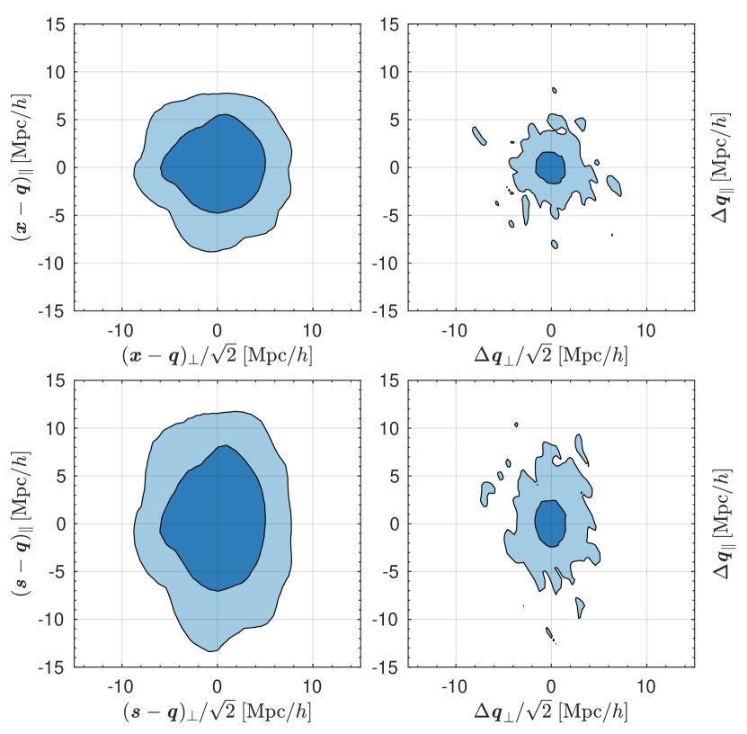
Figure 1: Lagrangian remapping accuracy of dark matter halos by the reconstructed simulation. The horizontal and vertical axes represent the errors of the perpendicular and parallel components of the line of sight. The left/right column is the errors before/after the reconstructed remapping, and the upper/lower row is with/without redshift space distortions. The inner and outer contours contain 68 and 95 percent of the halo population with mass $\geq 10^{12}M_{\odot}/h$, respectively.

With the reconstructed initial condition, we run a reconstructed simulation with $200^{3}$ particles, in order to recover the Lagrangian properties of halos in the original simulation. We label the estimated properties or the values in the reconstructed simulation by “$\ \hat{}\$”. The trajectories of the $N$-body particles in the reconstructed simulation provide a displacement field $\hat{\boldsymbol{\Psi}}(\hat{\boldsymbol{q}})\equiv\hat{\boldsymbol{x}}-\hat{\boldsymbol{q}}$, uniformly sampled at the Lagrangian positions $\hat{\boldsymbol{q}}$ of those particles, pointing to their final (Eulerian) positions $\hat{\boldsymbol{x}}$ at redshift $z=0$. Now we construct an inverse displacement field $\hat{\boldsymbol{\Phi}}(\hat{\boldsymbol{x}})\equiv\hat{\boldsymbol{q}}-\hat{\boldsymbol{x}}$ on a $200^{3}$ grid in order to remap halos back to their Lagrangian positions. However, the inverse displacement field is not uniformly sampled by $N$-body particles in Eulerian space; in the cosmic voids, there are many empty grids, and in the overdense regions, there are multiple particles falling in. To avoid having this vector field multivalued on a certain grid, we calculate the inverse displacement vector by averaging over all particles that are eventually located in the grid. For empty grids, their values are undefined or assigned with zero vectors, or alternatively, assigned with the inverse displacement vector of the last leaving particle, scaled by the linear growth factor up to redshift $z=0$. In practice, we find that how to deal with the empty grids does not affect the calculation of halo Lagrangian positions because all the halo positions in the original simulation $\boldsymbol{x}$ also correspond to positive overdensities in the reconstructed simulation. The inverse displacement field is then filtered by a Gaussian window function of scale $\sim 1.5\,{\rm Mpc}/h$, which we find it optimally reconstructs the Lagrangian properties in later sections.

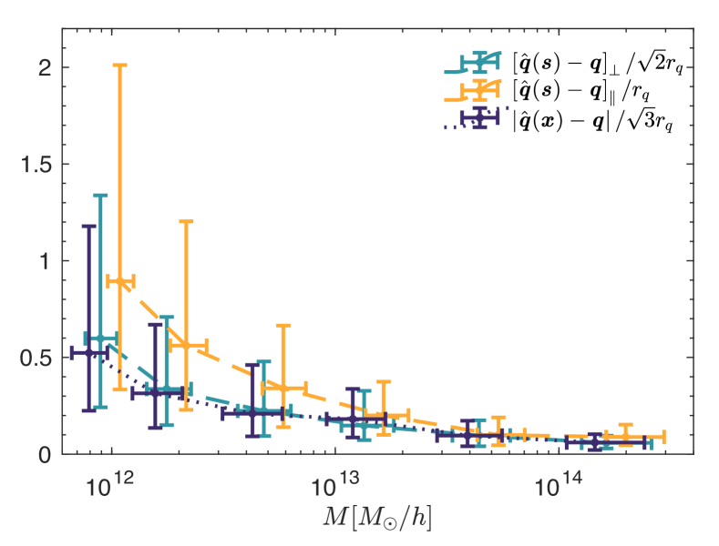
Figure 2: Relative remapping errors $\Delta q/r_{q}$ as a function of halo mass, with and without RSD effect. When RSD is included, the error components are plotted parallel and perpendicular to LoS, respectively. The purple dotted curve shows $1/\sqrt{3}$ times of relative errors $\Delta q/r_{q}$, when remapped directly from real space (without RSD). The yellow and cyan dashed curves show parallel components ($\Delta q_{\parallel}/r_{q}$) and $1/\sqrt{2}$ times the perpendicular components ($\Delta q_{\perp}/r_{q}$) of relative errors $\Delta q/r_{q}$, with RSD. All the points at the intersections show medians of data in each mass bin, and error bars are taken as $25\%$ and $75\%$ percentiles of the distribution.

For a given halo in Eulerian space $\boldsymbol{x}$, we interpolate its inverse displacement vector $\hat{\boldsymbol{\Phi}}(\boldsymbol{x})$ by the triangular shaped cloud (TSC) method (1981csup.book…..H, ) on the grid, and find the estimated Lagrangian position $\hat{\boldsymbol{q}}(\boldsymbol{x})=\boldsymbol{x}+\hat{\boldsymbol{\Phi}}(\boldsymbol{x})$, with RSD.

More realistically, halos and galaxies are initially observed in redshift space. We also calculate the redshift space coordinates of halos $\boldsymbol{s}=\boldsymbol{x}+\boldsymbol{u}_{\parallel}/aH$ according to their CoM peculiar velocities $\boldsymbol{u}$, where $\boldsymbol{u}_{\parallel}$ is the line of sight (LoS) component of $\boldsymbol{u}$, chosen here to be the second ($y$-) axis of the simulation. Although methods like ELUCID can identify galaxy groups and correct the redshift space distortions (RSD) (both the Kaiser (1987_kaiser, ) and finger of God effects), such that the halo positions are identified in real (Eulerian) space, here we also try to reconstruct the Lagrangian properties from the raw redshift space to study how RSD affects the spin reconstruction. In this case, the inverse displacement field is constructed on redshift space $\boldsymbol{s}$, i.e., $\hat{\boldsymbol{\Phi}}_{s}(\hat{\boldsymbol{s}})\equiv\hat{\boldsymbol{q}}-\hat{\boldsymbol{s}}$, and the Lagrangian position is reconstructed by $\hat{\boldsymbol{q}}(\boldsymbol{s})=\boldsymbol{s}+\hat{\boldsymbol{\Phi}}_{s}(\boldsymbol{s})$.

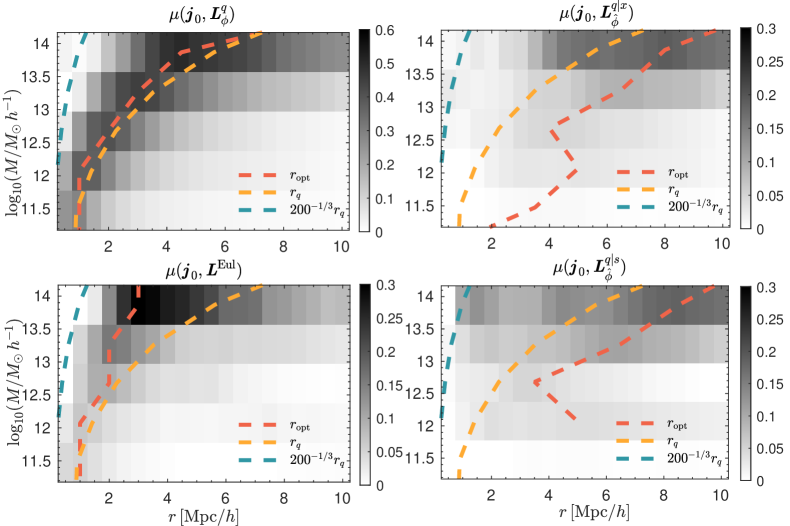
Figure 3: Optimal smoothing scale for spin reconstruction as a function of halo mass. The four panels show the cases of cross-correlating function $\mu(\boldsymbol{j}_{0},\boldsymbol{L}^{q}_{\phi})$ (top-left), $\mu(\boldsymbol{j}_{0},\boldsymbol{L}^{\rm Eul})$ (bottom-left), $\mu(\boldsymbol{j}_{0},\boldsymbol{L}_{\hat{\phi}}^{q|x})$ (top-right) and $\mu(\boldsymbol{j}_{0},\boldsymbol{L}_{\hat{\phi}}^{q|s})$ (bottom-right). The darker color of pixels means higher correlation and better reconstruction. The red and yellow curves are optimal smoothing scale $r_{\rm opt}$ and Lagrangian radius $r_{q}$. The cyan curve is $200^{-1/3}$ times the Lagrangian radius.

III Results

Here we quantify the results from the reconstructed simulation. First, we compare the remapped Lagrangian positions $\hat{\boldsymbol{q}}(\boldsymbol{x})$ and $\hat{\boldsymbol{q}}(\boldsymbol{s})$ with the true Lagrangian origins $\boldsymbol{q}$. Here we select halos with mass greater than $10^{12}M_{\odot}/h$. In the left column of Fig.1, the contours show the errors parallel ($\parallel$, vertical axis) and perpendicular ($\perp$, horizontal) to LoS, without the remapping process. The errors essentially come from the displacement of matter in the structure formation, and RSD brings additional errors in LoS direction. By using the reconstructed simulation, the halo positions are remapped back to Lagrangian coordinates with much better accuracy. The errors ($\Delta\boldsymbol{q}=\hat{\boldsymbol{q}}-\boldsymbol{q}$) are shown in the right column of Fig.1. The $1\sigma$ errors of the Lagrangian space remapping confirm to be $1.5{\rm Mpc}/h$ in perpendicular direction to line-of-sight and $2.5{\rm Mpc}/h$ in line-of-sight, which is much lower compared with errors without Lagrangian remapping, where the errors are $3.2{\rm Mpc}/h$ and $4.8{\rm Mpc}/h$. When the Lagrangian positions are remapped directly from the redshift space, the errors in LoS direction are slightly larger. The errors after remapping are mainly caused by the loss of small scale information in reconstructing the initial conditions.

The low redshift halos and galaxies can reflect the properties of their Lagrangian regions, which occupy a certain comoving volume. The errors of halo Lagrangian positions should be compared with the scale of those Lagrangian regions. Dark matter halos are the largest virialized objects in the universe, and their Lagrangian counterparts, the protohalos in Lagrangian space, are typically compact and simply connected. This is confirmed by our previous work (2023ApJ…943..128S, ). It is natural to use the Lagrangian equivalent radius $r_{q}\equiv(2MG/\Omega_{\rm m}H_{0}^{2})^{-1/3}$ to characterize this scale, where $M$, $G$, $\Omega_{\rm m}$, $H_{0}$ are the halo mass, Newton’s constant, current matter density parameter and the Hubble’s constant, respectively. Fig.2 shows the errors of Lagrangian remapping relative to each halo’s equivalent Lagrangian radius $r_{q}$. For the RSD contaminated case, these relative error vectors are plotted by LoS and transverse (perpendicular to LoS) components, and we divide all halos into six mass bins to show the mass dependence of the relative error. The centers of the error bars show the median of the distribution in each mass bin, while the left/lower and right/upper error bar boundaries show the $25\%$ and $75\%$ percentiles of the distribution. The general trend is that the relative remapping error $\Delta q/r_{q}$ is decreasing with the increase of halo mass. In particular, for halo masses greater than $10^{13}M_{\odot}/h$, the remapped Lagrangian positions are close to true values, with errors much smaller than the halo Lagrangian radii $r_{q}$. When the halo masses approach $10^{12}M_{\odot}/h$ or smaller, the errors are comparable to $r_{q}$. For the RSD contaminated case, we also plot the LoS and transverse error components separately. Note that if the error is isotropic, statistically $\Delta q_{\parallel}=\Delta q_{\perp}/\sqrt{2}$. The results show that halos with mass $\gtrsim 10^{13}M_{\odot}/h$ are uncontaminated by RSD, but for less massive halos, RSD brings additional uncertainties on $q_{\parallel}$ by about a factor of two.

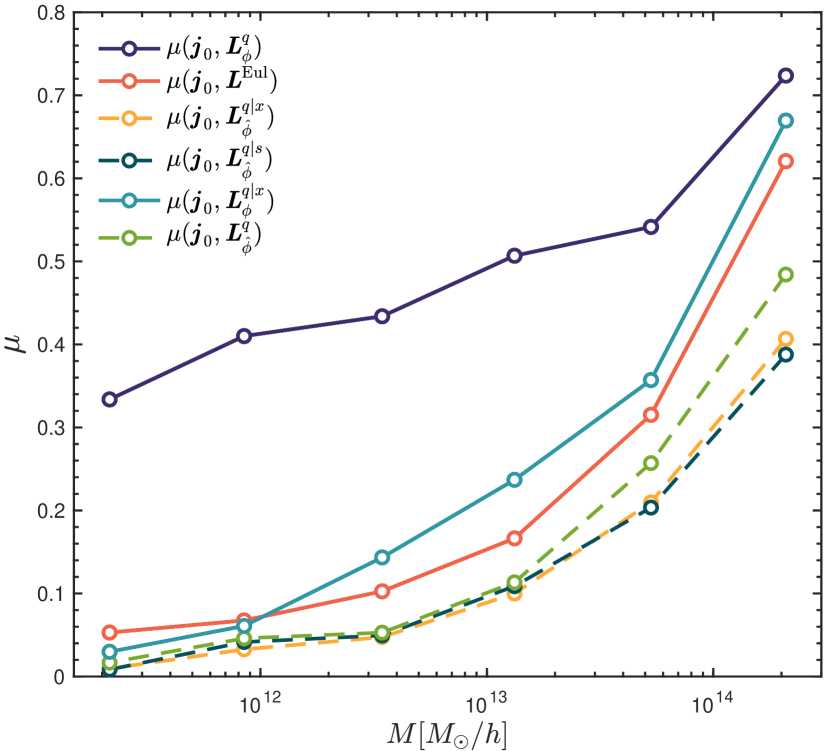
Figure 4: Maximally achievable cross-correlation of spin reconstruction of halos in different mass ranges. The spin reconstructed from $\boldsymbol{q}$ space ($\boldsymbol{L}^{q}_{\phi}$) and $\boldsymbol{x}$ space ($\boldsymbol{L}^{\rm Eul}$) in the original simulation is cross-correlated with $\boldsymbol{j}_{0}$, and the results are shown by the purple and red solid curves, respectively. The cross-correlations between the spin reconstructed from remapped coordinates $\boldsymbol{L}_{\hat{\phi}}^{q|x}$ and $\boldsymbol{L}_{\hat{\phi}}^{q|s}$ in the reconstructed simulation and $\boldsymbol{j}_{0}$ are illustrated by the yellow and dark cyan dashed curves. With or without the remapping process or the reconstructed initial condition are also plotted for comparison by cyan and green curves. Circles at the curves mean the maximum reachable cross-correlation at each halo bin.     

Next, we use the remapped Lagrangian positions and reconstructed primordial fluctuations to estimate the halo spin directions. Firstly, in the top left panel of Fig.3, we directly use Eq.(1), with the true Lagrangian positions and true tidal fields $T_{ij}\equiv\partial_{i}\partial_{j}\phi$ derived from the original initial potential field $\phi$. The cross correlation $\mu(\boldsymbol{j}_{0},\boldsymbol{L}^{q}_{\phi})$ are quantified by the cosine of the angle between the two angular momentum vectors. The gray scale plot illustrates $\mu$ as a function of the smoothing scale $r$ and the halo mass $M$. The red dashed curve shows the optimal smoothing scales $r_{\rm opt}$ which maximize $\mu$ in the given halo mass bins, while in this panel $r_{\rm opt}$ is compared with the Lagrangian equivalent radii $r_{q}$ (yellow dashed curve) and approximate halo scales $200^{-1/3}r_{q}$, which is the radius of a sphere whose mean density is 200 times the critical density of the Universe (cyan dashed curve). It is clear and expected that these two scales are similar for all halo mass bins. The correlation $\mu$ is high for all halo masses, while showing the slightly increasing function of $M$.

Next, we study the spin correlation using the reconstructed initial conditions (reconstructed potential $\hat{\phi}$) and the remapped Lagrangian coordinates. On the superscript, we use the symbol “$q|x$” to denote that the Lagrangian coordinate is estimated given the halo position $\boldsymbol{x}$, i.e., $\hat{\boldsymbol{q}}(\boldsymbol{x})$. Similarly, the superscript “$q|s$” stands for the estimated Lagrangian coordinate $\hat{\boldsymbol{q}}(\boldsymbol{s})$ given redshift position $\boldsymbol{s}$. On the subscript, we denote which potential field ($\phi$, $\hat{\phi}$, or $\phi_{0}$) is used for the spin reconstruction. For example, $\boldsymbol{L}_{\hat{\phi}}^{q|x}$ is the spin field reconstructed by $\hat{\phi}$ and $\hat{\boldsymbol{q}}(\boldsymbol{x})$, $\boldsymbol{L}_{{\phi}}^{q}$ means that the spin field is reconstructed by the real initial condition, and the halo spin is correlated with its real Lagrangian position in the field. $\boldsymbol{L}^{\rm Eul}$ is the spin reconstructed by $\phi_{0}$ and $\boldsymbol{x}$, i.e., $\boldsymbol{L}_{{\phi_{0}}}^{x}$.

Using remapped Lagrangian positions ($\hat{\boldsymbol{q}}(\boldsymbol{x})$ or $\hat{\boldsymbol{q}}(\boldsymbol{s})$) and the reconstructed initial conditions ($\hat{\phi}$), the spin field is correlated with the low redshift halo spin vectors, yielding the mean cross correlation $\mu(\boldsymbol{j}_{0},\boldsymbol{L}_{\hat{\phi}}^{q|x})$ and $\mu(\boldsymbol{j}_{0},\boldsymbol{L}_{\hat{\phi}}^{q|s})$ in each halo mass bin. They are plotted in the right two panels of Fig.3. Compared to the idealized linear spin reconstruction $\boldsymbol{L}_{{\phi}}^{q}$ (top left panel of Fig.3, where real $\phi$ as well as real $\boldsymbol{q}$ is used), the correlations decrease significantly across all mass ranges, by $30\%$ to $40\%$. For halos with mass $\gtrsim 10^{13}M_{\odot}/h$, corresponding to galaxy clusters, the correlation is still greater than $20\%$, while for less massive halos (about $10^{12}M_{\odot}/h$), the correlation drops to about $5\%$. Another feature is that the optimal smoothing scale $r_{\rm opt}$ is shifted to larger scales. This result directly explains the low correlation between observed galaxy spins and reconstructed cosmic initial conditions (ELUCID) in 2021_motloch_na , and the relatively large smoothing scale used there. Physically, the reconstructed initial condition loses correlation with the true initial condition on small scales, and thus the cosmic information is lost in this regime. Besides, the uncertainties on $\boldsymbol{q}$ also favor a larger $r_{\rm opt}$, such that the larger scale still-correlated tidal interactions can be included in the spin estimation. Comparing the two right panels of Fig.3, we find that RSD has an insignificant influence on the spin estimation.

It is instructive to investigate whether the tidal-torque based spin estimator also works in Eulerian space. Replacing the primordial tidal tensors $T_{ij}(\boldsymbol{q})$ with Eulerian values $T^{\rm Eul}_{ij}(\boldsymbol{x})\equiv\partial_{i}\partial_{j}\phi_{0}$, where $\phi_{0}$ is the Eulerian gravitational potential at $z=0$, and using the Eulerian positions $\boldsymbol{x}$, the Eulerian-space based spin estimator is written as

$$L^{\rm Eul}_{i}\propto\epsilon_{ijk}T^{\rm Eul}_{jl}({\boldsymbol{x}},r)T^{\rm Eul}_{lk}({\boldsymbol{x}},r{{}_{,+}}),$$ (2)

where $r$ is again the arbitrary smoothing scale. The result in the bottom left panel of Fig.3 shows that there are also correlation signals from the Eulerian-space based spin estimator. The correlations are found in all mass ranges but are significantly lower than in the Lagrangian space (top left panel). The other feature is that the optimal smoothing scale $r_{\rm opt}$ is somewhat located between $r_{q}$ and $200^{-1/3}r_{q}$. This may lead to the fact that the low redshift cosmic structures, especially on scales slightly larger than the halo scale, do have an influence on the halo angular momentum distribution and galaxy intrinsic alignments.

Lastly, we summarize the maximally achievable spin correlation $\mu_{\rm max}$ as a function of halo mass $M$. We calculate the cross-correlations between the $\boldsymbol{j}_{0}$ and the $\boldsymbol{L}$ reconstructed with several pairs of initial conditions and coordinates; specific definitions refer to Appendix A. In Fig.4, the top curve is obtained by the true initial condition $\phi$ and the true Lagrangian position $\boldsymbol{q}$, which is the idealized scenario given our spin reconstruction method. Its deviation from perfect correlation ($\mu=1$) comes from the approximations used in the tidal torque theory, spin reconstruction, and the nonlinear evolution. In practice, what we can use in the real space is the estimated $\hat{\phi}$ and remapped $\hat{\boldsymbol{q}}(\boldsymbol{s})$. Even $\hat{\boldsymbol{q}}(\boldsymbol{x})$ can only be derived with the permission of redshift distortion correction from $\boldsymbol{s}$. Comparing the two curves $\mu({\boldsymbol{j}}_{0},{\boldsymbol{L}}_{\hat{\phi}}^{q|x})$ and $\mu({\boldsymbol{j}}_{0},{\boldsymbol{L}}_{\hat{\phi}}^{q|s})$, we find that whether Lagrangian positions are remapped from real or redshift space has little effect on the upper limit of the cross-correlation – the RSD effect is well corrected in the remapping process.

The decreasing of the cross correlation comes from the combination of two effects – the error of remapping and the error of initial gravitational potential. In order to see which one is the dominant effect on the decorrelation, we plot the two curves $\mu({\boldsymbol{j}}_{0},{\boldsymbol{L}}_{\phi}^{q|x})$ and $\mu({\boldsymbol{j}}_{0},{\boldsymbol{L}}_{\hat{\phi}}^{q})$, i.e., using the true $\phi$ but estimated $\boldsymbol{q}$, and the true $\boldsymbol{q}$ but estimated $\phi$. It appears that the error on the initial potential $\phi$ has severer effects on spin reconstruction – the accuracy of the initial condition is more important than the accuracy of the remapping process in spin reconstruction. This shows the potential of better reconstruction of $\hat{\phi}$, given fixed $\hat{\boldsymbol{q}}(\boldsymbol{x})$, if additional spin information of galaxies/halos are used.

An additional curve $\mu({\boldsymbol{j}}_{0},{\boldsymbol{L}}^{\rm Eul})$ is also plotted in Fig.4 to show the maximally achievable correlation between low redshift halo spins and low redshift large scale structure. Although the Eulerian spin reconstruction is comparable to Lagrangian ones (with estimated quantities), it can not be straightforwardly used to reconstruct the initial perturbations. Nevertheless, it is closely related to galaxy/halo intrinsic alignments, and is additionally parity-odd. We leave this connection and physical explanation in future works.

IV conclusion and discussions

In this paper, by using the reconstructed simulations, we study the accuracy of Lagrangian space remapping – the initial comoving coordinates of virialized halo-galaxy systems are obtained. Inspired by the tidal torque theory, the halo angular momentum vector (spin) is reconstructed in Lagrangian space (spin reconstruction), and is used to assess the remapping quality. The main results are summarized as follows.

• The remapping process can remarkably reduce the errors induced by the displacement of matter in the structure formation, which is a crucial step in spin reconstruction. Statistically, the remapping errors are small compared to the Lagrangian radii of the protohalos, especially for massive ones.

• The correlation between halo spin and the reconstructed spin obtained from remapped coordinates and reconstructed initial gravitational potential drops compared to the idealized situation. The latter uses the true Lagrangian coordinates. The deviation significantly increases in low mass ranges, which explains the low correlation between observed galaxy spins and the spin reconstruction (and the optimal smoothing scale) in the real universe. RSD effect increases the remapping error parallel to the line of sight, but induces minor effects in the final spin reconstruction.

• The accuracy of the reconstructed initial gravitational potential is the main factor affecting the performance of the spin reconstruction, especially on small scales, while the remapping is relatively accurate.

Remapping the low-redshift observed objects back to Lagrangian space has profound importance in cosmology. Using the spin evolution of halo-galaxy systems as an example, the low-redshift spin vectors are reliable tracers of tidal environment of the protohalos. Observing the former infers the latter, and can further help obtaining the cosmic initial conditions. The displacement field relate these quantities at different coordinates – Eulerian (real or redshift space) and Lagrangian, and in this work we have shown that Eulerian space can be reliably remapped to Lagrangian space, can whose errors do not erase the spin correlation. The lowering of spin correlation is mainly due to the poor reconstruction of initial gravitational potential on small scales. Nevertheless, the initial gravitational potential is obtained by density reconstruction, which used only galaxy positions. By additionally using galaxy spins (especially the directions), the initial gravitational potential can be better constrained, and along with it, the displacement field, equivalently the Lagrangian remapping can be further improved. Iterating these steps can help obtaining a more accurate initial state of our universe, and we leave it in our subsequent works.

Appendix A Variable description

We present descriptions of the physical variables used in this paper in Table 1.

Table 1: Variables used in this paper.

Variables	Description
$\boldsymbol{q}$	True Lagrangian space coordinates
$\boldsymbol{x}$	Eulerian space coordinates
$\boldsymbol{s}$	Redshift space coordinates
$\hat{\boldsymbol{q}}$	$\boldsymbol{q}$ in reconstructed simulations
$\hat{\boldsymbol{\Psi}}(\boldsymbol{q})$	Displacement field
$\hat{\boldsymbol{\Phi}}(\boldsymbol{x})$, $\hat{\boldsymbol{\Phi}}(\boldsymbol{s})$	Inverse displacement field
$\boldsymbol{j}_{0}$	Eulerian spin vector
$\Delta{\boldsymbol{q}}$	$\boldsymbol{q}-\hat{\boldsymbol{q}}$
$r_{q}$	Lagrangian radius
$r_{\rm opt}$	Optimal smoothing scale
$\phi$	Gravitation field in Lagrangian space
$\phi_{0}$	Gravitation field in Eulerian space
$\hat{\phi}$	Reconstructed initial gravitation field
$\epsilon_{ijk}$	Levi-Civita symbol
$I_{ij}$	Momentum of inertia tensor of the protohalo
$T_{ij}$	Tidal tensor field
$\boldsymbol{L}^{\rm Eul}$	Spin reconstructed by $\phi_{0}$ and $\boldsymbol{x}$
$\boldsymbol{L}^{q}_{\phi}$	Spin reconstructed by the $\phi$ and $\boldsymbol{q}$
$\boldsymbol{L}^{q}_{\hat{\phi}}$	Spin reconstructed by the $\hat{\phi}$ and $\boldsymbol{q}$
$\boldsymbol{L}^{q|x}_{\hat{\phi}}$	Spin reconstructed by the $\hat{\phi}$ and $\hat{\boldsymbol{q}}(\boldsymbol{x})$
$\boldsymbol{L}^{q|s}_{\hat{\phi}}$	Spin reconstructed by the $\hat{\phi}$ and $\hat{\boldsymbol{q}}(\boldsymbol{s})$
$\boldsymbol{L}^{q|x}_{\phi}$	Spin reconstructed by the $\phi$ and $\hat{\boldsymbol{q}}(\boldsymbol{x})$

References

- (1) C. D. Rimes and A. J. S. Hamilton, MNRAS360, L82 (2005), astro-ph/0502081.
- (2) M. McQuinn, J. Cosmology Astropart. Phys2021, 024 (2021), 2008.12312.
- (3) P. J. E. Peebles, ApJ155, 393 (1969).
- (4) S. Dodelson and F. Schmidt, Modern Cosmology (, 2020).
- (5) H.-R. Yu, U.-L. Pen, and H.-M. Zhu, Phys. Rev. D95, 043501 (2017), 1610.07112.
- (6) Q. Pan, U.-L. Pen, D. Inman, and H.-R. Yu, MNRAS469, 1968 (2017), 1611.10013.
- (7) N. Turok, U.-L. Pen, and U. Seljak, Phys. Rev. D58, 023506 (1998), astro-ph/9706250.
- (8) A. G. Doroshkevich, Astrofizika 6, 581 (1970).
- (9) S. D. M. White, ApJ286, 38 (1984).
- (10) P. Motloch, H.-R. Yu, U.-L. Pen, and Y. Xie, Nature Astronomy 5, 283 (2021), 2003.04800.
- (11) H. Wang, H. J. Mo, X. Yang, Y. P. Jing, and W. P. Lin, ApJ794, 94 (2014), 1407.3451.
- (12) H. Wang et al., ApJ831, 164 (2016), 1608.01763.
- (13) H.-R. Yu et al., Phys. Rev. Lett.124, 101302 (2020), 1904.01029.
- (14) Q. Wu, H.-R. Yu, S. Liao, and M. Du, Phys. Rev. D103, 063522 (2021), 2011.03893.
- (15) M.-J. Sheng et al., ApJ943, 128 (2023), 2210.04203.
- (16) Q. Wu, H.-R. Yu, S. Liao, and M. Du, Phys. Rev. D103, 063522 (2021), 2011.03893.
- (17) A. F. Teklu et al., ApJ812, 29 (2015), 1503.03501.
- (18) H.-R. Yu et al., Phys. Rev. Lett.124, 101302 (2020), 1904.01029.
- (19) D. H. Weinberg, MNRAS254, 315 (1992).
- (20) J. Einasto et al., A&A531, A75 (2011), 1012.3550.
- (21) H. Rein and D. Tamayo, MNRAS473, 3351 (2018), 1704.07715.
- (22) X. Wang et al., ApJ841, L29 (2017), 1703.09742.
- (23) R. Mohayaee, U. Frisch, S. Matarrese, and A. Sobolevskii, A&A406, 393 (2003), astro-ph/0301641.
- (24) H. Wang, H. J. Mo, X. Yang, and F. C. van den Bosch, ApJ772, 63 (2013), 1301.1348.
- (25) J. Dunkley et al., ApJS180, 306 (2009), 0803.0586.
- (26) H.-R. Yu, U.-L. Pen, and X. Wang, ApJS237, 24 (2018), 1712.06121.
- (27) Y. B. Zel’dovich, A&A5, 84 (1970).
- (28) R. W. Hockney and J. W. Eastwood, Computer Simulation Using Particles (, 1981).
- (29) M. Davis, G. Efstathiou, C. S. Frenk, and S. D. M. White, ApJ292, 371 (1985).
- (30) F. Qin, D. Parkinson, S. E. Hong, and C. G. Sabiu, J. Cosmology Astropart. Phys2023, 062 (2023), 2302.02087.
- (31) C. Modi, Y. Li, and D. Blei, J. Cosmology Astropart. Phys2023, 059 (2023), 2206.15433.
- (32) C. J. Shallue and D. J. Eisenstein, MNRAS520, 6256 (2023), 2207.12511.
- (33) V. Jindal, A. Liang, A. Singh, S. Ho, and D. Jamieson, arXiv e-prints , arXiv:2303.13056 (2023), 2303.13056.
- (34) N. Kaiser, MNRAS227, 1 (1987).