Effect of realistic oscillator phase noise on the performance of cell-free networks

Abstract

To keep supporting 6G requirements, the radio access infrastructure will increasingly densify. Cell-free (CF) networks offer extreme flexibility by coherently serving users with multiple Access points (APs). This paradigm requires precise and stable phase synchronization. In this article, we adapt the standardized 5G NR setup (subcarrier spacing, OFDM symbol duration and allocation) to investigate the effect of Phase Noise (PN) on the simulated performance of scalable CF networks. In contrast to the prior literature relying on the simplified model of a free-running oscillator with the Wiener process, we deploy a realistic hardware-inspired phase noise model reproducing the Local Oscillator (LO) phase drift. Our results demonstrate that even affordable LOs offer sufficient stability to ensure negligible loss of uplink Spectral Efficiency (SE) on the time scale of the standardized 5G Transmission Time Interval of 1 ms. This study substantiates the feasibility of CF networks based on 5G standards.

I Introduction

Cell-free (CF) networking will play a pivotal role in the upcoming 6G networks [1, 2]. In CF, user devices (often called ”User Equipment” or UE) are served by multiple Access Points (APs) performing coherent joint transmission and reception [3]. This approach offers superior Spectral Efficiency (SE) compared to conventional architectures like Macro Base Stations or small cells [4], promising a more efficient and effective network infrastructure for 6G.

CF networking has attracted attention for its impressive performance in theoretical studies under ideal conditions [4]. Building upon this success, subsequent research has focused on incorporating more realistic assumptions, including the utilization of non-ideal hardware, to facilitate practical implementation. These efforts can be categorized into two main groups: 1) hardware implementations or testbeds aimed at validating and demonstrating the feasibility of CF networking in real-world scenarios, and 2) analytical and simulation studies that employ more realistic assumptions. Since the main enabler of the CF is coherent processing, here we would like to underline the importance of phase synchronization between the communication nodes (e.g., a UE and APs serving the user, including inter-AP synchronization).

Testbeds

Wang et al. [5] implemented a centralized cloud-based CF mMIMO network. In their testbed, a CPU served 16 eight-antenna UEs with 16 eight-antenna APs. In [6], the KU Leuven CF Multiple-Input-Multiple-Output (MIMO) testbed was used to obtain channel state information (CSI) in a dense CF deployment consisting of 8 APs with 8 antennas each (64 antennas in total). In both works, most of the Hardware Impairments (HWI) effects are implicitly assessed since real equipment was used. Unfortunately, both works used a common clock and the effect of Phase Noise (PN) was not estimated.

Theoretical studies

Several works investigated the effect of Local Oscillator (LO) PN on a single carrier [7, 8] and on OFDM-based [9] CF networks. The articles assess the performance of CF networks when non-ideal LOs are used. Inspired by Petrovic et al. [10], the authors of the papers modeled PN by a discrete-time independent Wiener process assuming independent innovations at every time instance. The papers reported significant degradation in comparison to an ideal LO: up to 58% performance degradation in terms of 5%-outage rate in [8]. The authors of [7, 9] propose channel estimators compensating for PN in the sense of estimating the effective channel. By utilizing the assumed structure of PN in the estimator and then using the estimate for receive combining, a sort of phase noise compensating signal processing framework was proposed.

Stat-of-the-Art limitations: The PN model used in [7, 8, 9] is a good choice for a first approximation of real LO performance. However, considering the immense importance of coherent processing for the potential of CF, more realistic PN models must be used to assess the CF network performance as it was highlighted by practitioners [11].

Contributions: In this work, we

1. Critically analyze the impact of time-frequency resource allocation specified by 3GPP on PN.

2. Deploy a realistic hardware-inspired phase noise model reproducing the LO phase drift.

3. Simulate a CF network to assess the effect of realistic PN on uplink SE of 3GPP-compliant OFDM system.

Notation: Vectors and matrices are denoted by boldface lower and upper case symbols. The symbols $(\cdot)^{T}$, $(\cdot)^{H}$, and $(\cdot)^{\dagger}$ express the transpose, Hermitian transpose, and pseudo-inverse operators, respectively. The notations $\mathbb{C}^{L\times 1}$ and $\mathbb{C}^{W\times W}$ refer to complex $L$-dimensional vectors and $W\times W$ matrices, respectively. Finally, $\mathbf{a}\sim\mathcal{CN}(0,\mathbf{\Sigma})$ represents a circularly symmetric complex Gaussian variable with zero mean and covariance matrix $\mathbf{\Sigma}$.

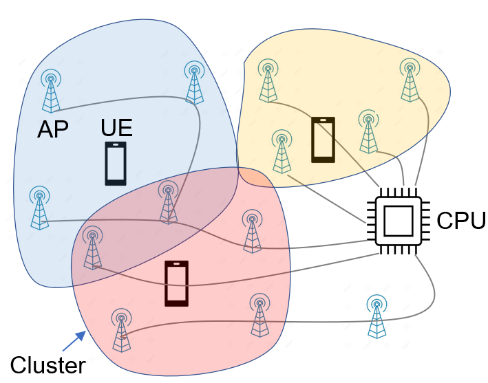
Figure 1: CF massive MIMO network with user-centric clustering.

II System Model

First, we introduce the OFDM system model considering PN effects. Secondly, we adopt standard 3GPP settings and show their effect on the expected influence of PN. Finally, we introduce the scalable CF network model taking into account the realistic effects of PN on the OFDM system.

Industry-baked efforts targeting the development of CF networks are heavily based on 5G NR standards [12, 13] to simplify the transition to practice. In this article, we use the same approach. To focus solely on the communication performance, we assume that the Initial Access, Pilot Assignment, Cluster Formation, Channel Estimation, and Radio Resource Allocation procedures are completed by utilizing techniques available in the literature [14, 15].

II-A OFDM system model

Consider an OFDM system with $N$ subcarriers, a subcarrier spacing $\Delta f$, and a bandwidth $B=1/T_{\rm s}=N\Delta f$, where $T_{s}$ is the sampling period. Signal $\{X_{i}\}_{i=0}^{N-1}$ is transmitted over $N$ subcarriers of an OFDM symbol, with an average per-symbol power $p$. By means of an $N$-point IDFT, we can write the time-domain representation of the OFDM symbol transmitted by UE as

$$x_{n}={\frac{1}{\sqrt{N}}}{\sum_{i=0}^{N-1}}X_{i}e^{j2\pi in/N},$$ (1)

where index $n$ is the time-domain channel use (sample).

II-A1 Phase Noise Model

Time-dependent random phase drifts, also known as PN, cause multiplicative distortions of the received signal. The distortions are introduced when the signal is multiplied by the LO’s output during up- and down-conversion operations.

The total PN between one user and one AP at $n$-th time sample can be expressed as

$$\theta_{n}=\phi_{n}+\varphi_{n}.$$ (2)

The particular realizations of the $\phi_{n}$ and $\varphi_{n}$ depend on the model, e.g. it can be a simple Wiener process or a random process with a complex spectrum defined by various instabilities of the LOs (phase noise, phase random walk, frequency noise, frequency random walk etc.). The models of the phase noise are discussed in details in Sec. III.

We can express time-domain PN realization during one received OFDM symbol as $\mathbf{p}^{\rm{time}}=[e^{j\theta_{0}},\dots,e^{j\theta_{N-1}}]^{T}\in\mathbb{C}^{N\times 1}$ while its frequency-domain counterpart is written as $\mathbf{p}^{\rm{freq}}=[P_{0},\dots,P_{N-1}]^{T}\in\mathbb{C}^{N\times 1}$ where the elements are obtained via DFT as $P_{i}=\frac{1}{N}\sum_{n=0}^{N-1}e^{j\theta_{n}}e^{-j2\pi ni/N}$.

II-A2 OFDM Signal Model with Phase Noise

The received signal in the time domain ${\mathbf{y}^{\rm{time}}}\in\mathbb{C}^{N\times 1}$ is

$$\begin{split}{\mathbf{y}^{\rm{time}}}&=\mathbf{p}^{\rm time}\circ({\mathbf{x}^{\rm{time}}}\circledast{\mathbf{h}^{\rm{time}}})+{\mathbf{z}^{\rm{time}}},\end{split}$$ (3)

where $\mathbf{x}^{\rm{time}}\in\mathbb{C}^{N\times 1}$ the transmitted signal, $\mathbf{h}^{\rm{time}}\in\mathbb{C}^{N\times 1}$ the channel impulse response, and ${\mathbf{z}^{\rm{time}}}\in\mathbb{C}^{N\times 1}$ the additive white Gaussian noise (AWGN) with i.i.d. ${\mathcal{CN}}\left(0,\sigma_{z}^{2}\right)$ elements. It is easy to show that, the received signal in the frequency domain ${\mathbf{y}^{\rm{freq}}}\in\mathbb{C}^{N\times 1}$ is

$$\begin{split}{\mathbf{y}^{\rm{freq}}}&={\mathbf{p}^{\rm{freq}}}\circledast({\mathbf{x}^{\rm{freq}}}\circ{\mathbf{h}^{\rm{freq}}})+{\mathbf{z}^{\rm{freq}}}\end{split}$$ (4)

where $\mathbf{x}^{\rm{freq}}=[X_{0},X_{1},\cdots,X_{N-1}]^{\rm T}$, $\mathbf{h}^{\rm{freq}}=[H_{0},H_{1},\cdots,H_{N-1}]^{\rm T}$, $\mathbf{z}^{\rm{freq}}=[Z_{0},Z_{1},\cdots,Z_{N-1}]^{\rm T}\in\mathbb{C}^{N\times 1}$ are the transmit symbol, channel frequency response, and noise, respectively, in the frequency domain.

PN effects on the received signal for each subcarrier $i\in\{0,1,\cdots,N-1\}$, (4) can be rewritten as [16]

$$Y_{i}=\underbrace{P_{0}}_{\rm CPE}H_{i}X_{i}+\underbrace{{\sum_{\ell=0,\ell\neq i}^{N-1}}P_{(i-\ell)_{N}}H_{\ell}X_{\ell}}_{\rm ICI}+Z_{i},$$ (5)

where $(\cdot)_{N}$ denotes the modulo-$N$ operation. The Common Phase Error (CPE) is an identical phase rotation in all subcarriers within an OFDM symbol while the Inter-Carrier Interference (ICI) is an additive noise (not always Gaussian). Note that for a given OFDM symbol, CPE can be estimated and compensated during the channel estimation process.

II-A3 Channel Model

We consider a time-varying channel that is divided into Coherence Blocks (CBs) with a coherence time $T_{\rm c}$ and a coherence bandwidth $B_{\rm c}$. Within the coherence time, $N_{\rm ct}\triangleq\lfloor{T_{\rm c}}/{T_{\rm OFDM}}\rfloor$ OFDM symbols with duration $T_{\rm OFDM}$ are transmitted. Similarly, we can calculate the number of subcarriers within the coherence bandwidth as $N_{\rm cb}\triangleq\lfloor{B_{\rm c}}/{\Delta f}\rfloor$. Each CB spans $N_{\rm ct}$ and $N_{\rm cb}$ successive OFDM symbols and subcarriers, over which the channel is time-invariant and frequency flat. In the following, let us consider one coherence block as the focus of our analysis.

Numerology: For the Frequency Range 1 (FR1: sub-6 GHz), the most popular 5G NR numerology is $\mu=0$, consequently, the smallest time-frequency resource unit that can be scheduled to a user corresponds to a CB spanning over $B_{\rm c}$=180 kHz bandwidth ($N_{\rm cb}=12$ subcarriers with $\Delta f=15$ kHz spacing) and $T_{\rm c}=1$ ms (divided into $N_{\rm ct}=14$ OFDM symbols with a duration of $T_{\rm OFDM}=$71.4 $\mu$s each). The number of coherent channel uses is $\tau=N_{\rm ct}N_{\rm cb}$.

II-A4 Resource Element Mapping and Channel Estimation

In line with [15], we assume the Transmission Time Interval (TTI) format where all OFDM symbols are used for uplink communication. To enable channel estimation and CPE compensation, at least one OFDM symbol should contain pilot signals (Demodulation Reference Signal) according to 3GPP TS 38.211. Though most commonly OFDM symbols 3 or 4 are used, we can assume a scenario where the pilots are transmitted at the very beginning of the TTI (see Fig. 2). The coherent channel uses $\tau=\tau_{p}$ and $\tau_{c}$ consist of channel uses for pilot and data, respectively.

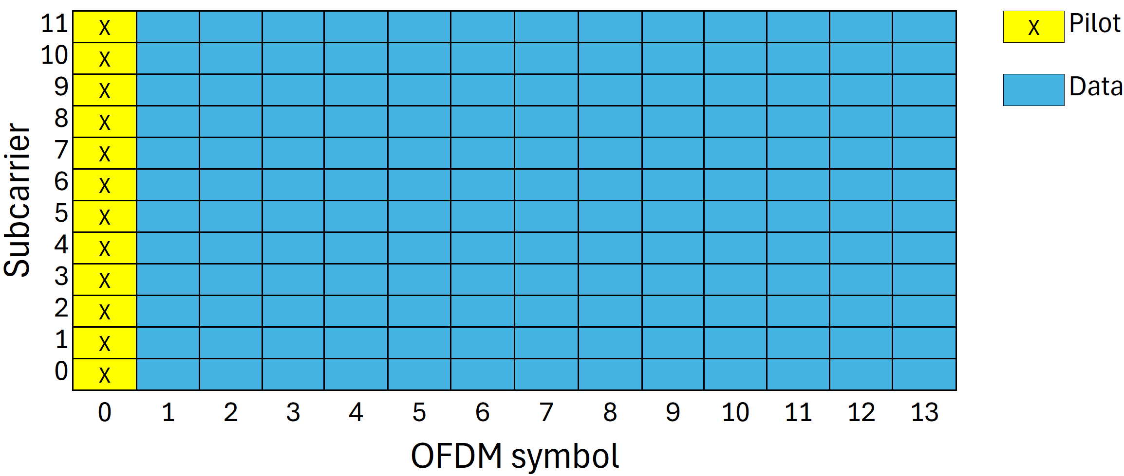
Figure 2: Mapping of the Resource Elements within a coherence block.

The pilot allocation in Fig. 2 represents the worst-case scenario from the CPE point of view. The CPE is compensated only at $\mathfrak{t}=0$ OFDM symbol while the other symbols are affected by the growing error. For an arbitrary OFDM symbol $\mathfrak{t}$, the received signal is expressed as:

$$Y_{i}^{\mathfrak{t}}=P_{0}^{\mathfrak{t}}HX_{i}^{\mathfrak{t}}+Z_{i}^{\mathfrak{t}},$$ (6)

where $P_{0}^{\mathfrak{t}}$ is the CPE for the OFDM symbol $\mathfrak{t}$ (note that $P_{0}^{0}=1$) and $H$ is constant over $N_{\rm ct}$ OFDM symbols and $N_{\rm cb}$ subcarriers. Compared to (5), this equation also takes into account that the 5G subcarrier spacing aims at eliminating the effect of ICI.

II-B Scalable Cell-Free network

The CF massive MIMO (CF mMIMO) network shown in Fig. 1 is a communication network consisting of $M$ APs distributed over a geographical area that collaborate to serve $K$ users through coherent joint transmission and reception [3] utilizing shared time-frequency resources. The APs are connected to central processing units (CPUs) responsible for coordination. Precoding and combining operations can be performed at each AP, centrally at the CPU, or through a distributed approach involving both APs and CPUs [6]. In this study, we focus on the centralized processing.

II-B1 CF Channel model

Let us consider a general case of APs equipped with $L$ antennas and extend the model in Sec II-A3. Within a coherence block, the random channel vector between UE $k$ and AP $m$ is modeled by independent correlated Rayleigh fading as $\mathbf{h}_{mk}\sim\mathcal{CN}(0,\mathbf{R}_{mk})$ where the small scale fading is modeled with complex Gaussian distribution and $\mathbf{R}_{mk}\in\mathbb{C}^{L\times L}$ is a deterministic positive semi-definite correlation matrix that describes the large-scale propagation effects (i.e., shadowing and pathloss) with a fading coefficient $\beta_{mk}=tr(\mathbf{R}_{mk})/L$. Similarly to [4, 7], we assume that the set of correlation matrices is known by the communication nodes.

II-B2 Scalable CF

To ensure network scalability, each AP serves just a set of UEs. Björnsson and Sanguinetti [4] suggested forming clusters of APs serving users in a user-centric manner (see Fig. 1). In this case, AP $m$ serves just a subset of $K$ UEs ensuring the network scalability

$$\mathcal{D}_{m}=\{k:\quad\mathrm{tr}(\mathbf{D}_{mk})\geq 1,\quad k\in\{1,\dots,K\}\}.$$ (7)

II-B3 Phase Noise in CF

Since there is no ICI, phase noise should be updated once per OFDM symbol $\mathfrak{t}$ which corresponds to an update of CPE every $T_{\rm OFDM}$. For a practical scenario where $L$ antennas of the $m$-th AP are connected to a single LO, the corresponding PN matrix for $k$-th UE is expressed as $\mathbf{\Theta}_{mk}^{\mathfrak{t}}=e^{j\theta_{mk}^{\mathfrak{t}}}\mathbf{I}_{L}$, where $\theta_{mk}^{\mathfrak{t}}$ is obtained as in (2) for AP $m$ and UE $k$. Note that $\mathbf{\Theta}_{mk}^{0}=\mathbf{I}_{L}$ as CPE for $\mathfrak{t}=0$ is included in the channel estimation.

II-B4 Received Signal Model

Here we derive the achievable SE for a practical scalable CF network with PN. We use centralized processing, where the APs forward all received signals to the CPU. Next, the CPU performs the channel estimation and data detection. Note that to isolate the negative effects of channel estimation error from the effects introduced by PN, we assume perfect channel estimation.

In uplink, the $M$ APs send the received signals $\{\mathbf{y}_{m,i}:m=1,\cdots,M\}$ to the CPU. In such case by setting $W=ML$, the uplink signal received on $i$-th subcarrier of the given ODFM symbol can be written as

$$\mathbf{y}_{i}=\sum_{k=1}^{K}\mathbf{\Theta}_{k}\mathbf{h}_{k}X_{k,i}+\mathbf{n},$$ (8)

where $X_{k,i}\in\mathbb{C}$ from UE $k$ with power $p_{k}$, $\mathbf{y}_{i}=[\mathbf{y}_{1,n}^{T}\cdots\mathbf{y}_{M,n}^{T}]^{T}\in\mathbb{C}^{W\times 1}$ is a block vector, while $\mathbf{h}_{k}=[\mathbf{h}_{k1}^{T}\cdots\mathbf{h}_{kM}^{T}]^{T}\sim\mathcal{CN}(\mathbf{0},\mathbf{R}_{k})$ is the concatenated channel vector from all APs and $\mathbf{\Theta}_{k}=\mathrm{diag}(\mathbf{\Theta}_{1k},\cdots,\mathbf{\Theta}_{Mk})\in\mathbb{C}^{W\times W}$ is the phase noise matrix including CPE for this OFDM symbol. The block diagonal spatial correlation matrix $\mathbf{R}_{k}=\mathrm{diag}(\mathbf{R}_{k1},\cdots,\mathbf{R}_{kM})\in\mathbb{C}^{W\times W}$ is obtained by assuming that the channel vectors of different APs are independently distributed. Finally, the thermal noise vector $\mathbf{n}\sim\mathcal{CN}(0,\sigma^{2}_{W}\mathbf{I}_{W})$ is spatially and temporally independent and has variance $\sigma_{W}$. We define the effective channel for the ${\mathfrak{t}}$-th OFDM symbol (including the CPE) as $\tilde{\mathbf{h}}^{\mathfrak{t}}=\mathbf{\Theta}^{\mathfrak{t}}\mathbf{h}$.

As we stated before, although all APs receive the signals from all UEs, only a subset of the APs contributes to signal detection. Thus, the network estimates of $X_{k,i}$ are

$$\begin{split}\hat{X}_{k,i}&=\sum_{m=1}^{M}\mathbf{v}_{mk}^{H}\mathbf{D}_{mk}\mathbf{y}_{m,i}\\ &\!=\!\underbrace{\mathbf{v}_{k}^{H}\mathbf{D}_{k}\tilde{\mathbf{h}}_{k}X_{k}}_{Desired~{}signal}\!+\!\!\!\underbrace{\sum_{\ell=1,\ell\neq k}^{K}\!\!\!\mathbf{v}_{k}^{H}\mathbf{D}_{k}\tilde{\mathbf{h}}_{\ell}X_{\ell}}_{Multi-user~{}interference}\!+\mathbf{v}_{k}^{H}\mathbf{D}_{k}\mathbf{n}\end{split}$$ (9)

with $\mathbf{v}_{k}=\left[\mathbf{v}_{1}^{T}\cdots\mathbf{v}_{M}^{T}\right]^{T}\in\mathbb{C}^{W\times 1}$ being the collective combining vector and $\mathbf{D}_{k}=\mathrm{diag}\left(\ \mathbf{D}_{1k},\ldots,\mathbf{D}_{Mk}\right)\in\mathbb{C}^{W\times W}$ being a block diagonal matrix while the bottom version of the equation is obtained from the top one in terms of collective vectors.

In this paper, we use Maximum Ratio (MR) and Minimum Mean-Square Error (MMSE) given as

$$\mathbf{v}_{k}^{\text{MR}} =\mathbf{D}_{k}\hat{\mathbf{h}}_{k}$$ (10)

$$\mathbf{v}_{k}^{\text{MMSE}} =p_{k}\Big{(}\sum\limits_{\ell=1}^{K}p_{\ell}\hat{\mathbf{H}}_{\ell}^{D}+\mathbf{Z}_{k}\Big{)}^{\dagger}\mathbf{D}_{k}\hat{\mathbf{h}}_{k},$$ (11)

where $p_{k}$ is the transmit power of user $k$, $\hat{\mathbf{H}}_{\ell}^{D}=\mathbf{D}_{k}\hat{\mathbf{h}}_{\ell}\hat{\mathbf{h}}_{\ell}^{H,}\mathbf{D}_{k}$ and $\mathbf{Z}_{k}=\mathbf{D}_{k}\big{(}\sum_{\ell=1}^{K}p_{i}\mathbf{R}_{i}+\sigma_{\text{}}^{2}\mathbf{I}_{L}\big{)}\mathbf{D}_{k}$.

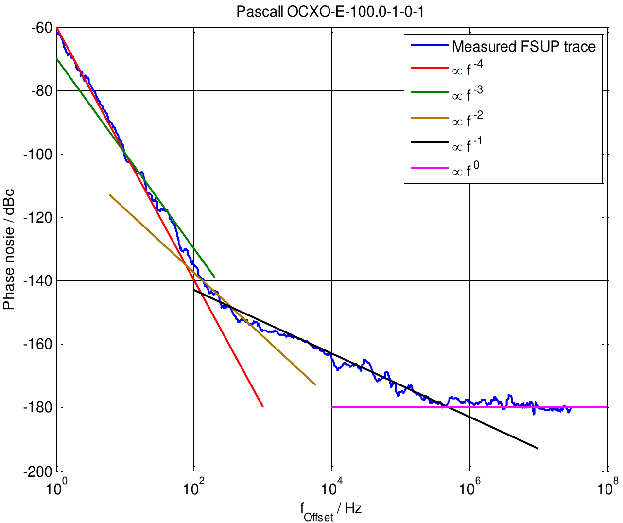
Figure 3: PSD of an ovenized crystal oscillator (OCXO) phase noise versus frequency offset with asymptots corresponding to different noise parts: phase white noise $~{}\sim f^{0}$, phase flicker noise $~{}\sim f^{-1}$, frequency white noise $~{}\sim f^{-2}$, frequency flicker noise $~{}\sim f^{-3}$, frequency random walk $~{}\sim f^{-4}$. Courtesy of Rohde&Schwarz [17].

Finally, an achievable SE of UE $k$ for OFDM symbol $\mathfrak{t}$ is

$$\text{SE}_{k}^{\mathfrak{t}}=\log_{2}(1+\text{SINR}_{k}^{\mathfrak{t}}),$$ (12)

where Signal to Interference and Noise Ratio (SINR) is given by (13). The SE expression in (12) can be computed numerically for any combiner $\mathbf{v}_{k}$. Note that SE changes for each OFDM symbol due to the CPE.

$$\text{SINR}_{k}^{\mathfrak{t}}=\frac{p_{k}\left|\mathbb{E}\left\{\mathbf{v}_{k}^{H}\mathbf{D}_{k}\tilde{\mathbf{h}}_{k}^{\mathfrak{t}}\right\}\right|^{2}}{\sum\nolimits_{\ell=1}^{K}p_{\ell}\mathbb{E}\Big{\{}\left|\mathbf{v}_{k}^{H}\mathbf{D}_{k}\tilde{\mathbf{h}}_{\ell}^{\mathfrak{t}}\right|^{2}\Big{\}}-p_{k}\left|\mathbb{E}\Big{\{}\mathbf{v}_{k}^{H}\mathbf{D}_{k}\tilde{\mathbf{h}}_{k}^{\mathfrak{t}}\right\}\Big{|}^{2}+\sigma^{2}\mathbb{E}\Big{\{}\left|\mathbf{D}_{k}\mathbf{v}_{k}^{H}\right|^{2}\Big{\}}}$$ (13)

 

III Phase Noise Model

In this section, we will first present a simplified PN phase model commonly found in the literature (Sec. III-A). Then, to create a realistic PN model we refer to the practical implementation of the Software Defined Radio (SDR) transceivers. In Sec. III-C, we briefly describe the contributions to PN introduced by different components of an LO. We conclude the section with presenting data of the real devices we use for the modeling in Sec. III-D.

III-A Simplified PN Model: Free Running Oscillator

As a reference, we use a model where the phase follows Weiner process [10] described by $\phi_{m}(t)\sim\mathcal{N}(\phi_{m}(t-1),\sigma^{2}_{\phi})$ and $\varphi_{k}(t)\sim\mathcal{N}(\varphi_{k}(t-1),\sigma^{2}_{\varphi})$, where $t$ denotes the channel use number while the variance of innovation can be expressed by [10]

$$\sigma_{x}^{2}=4\pi^{2}f^{2}_{c}c_{x}T_{\rm OFDM},$$ (14)

where $x$ is to be replaced by $\phi$ or $\varphi$ while $f_{c},c_{x}$ and $T_{\rm OFDM}$ are the carrier frequency, an oscillator-specific constant, and the symbol interval, respectively.

III-B Hardware-Inspired Phase Noise Model

To make the PN modeling more accurate and realistic, we implement a model of real-world devices. We consider SDRs transceivers which use LOs used for frequency up-/downconversion and sample I/Q at baseband. In our model, a LO is a voltage-controlled oscillator (VCO) which is locked to a reference crystal oscillator (XO) by a phase-locked loop (PLL). This model allows us to precisely model the behavior of many common SDRs which are based on integrated transceiver chips (e.g., Analog Devices AD9361). We also apply this model to more complex SDRs which may have multiple PLL stages to filter the reference clock and generate the sampling and carrier frequency (e.g. Ettus USRP X300 series). In the latter case, we limit our consideration to the last VCO+PLL (the one that generates the actual carrier frequency) and to one XO.

III-C Phase Noise Model of a Local Oscillator

To describe a PN of a standalone oscillator, the engineering community uses one-sided Power Spectral Density (PSD) $S(\delta f)$ where $\delta f$ is the frequency offset from the carrier frequency. Depending on the considered time scale, $\delta f$ can go down to fractions of Hertz (corresponding to time intervals of a second and more) and up to hundredss of MHz (when we consider period-to-period jitter of a carrier).

Different sources of PN prevail at different time scales: white and flicker noises of phase at high $\delta f$, white and flicker noises of frequency, and frequency random walk at slowest time scales. An example of contributions of these noise types can be seen in Fig. 3.

Naturally, XOs have good stability at long time scales and moderate PN at high $\delta f$. At the same time, they cannot be used for directly generating frequencies over $\sim 100$ MHz. The frequency can be multiplied to get the carrier frequency $f_{c}$, but the PN amplitude increases proportionally to the carrier frequency as

$$S_{f_{c}}(\delta f)=S_{\mathrm{XO}}(\delta f)\cdot f_{c}/f_{\mathrm{XO}}.$$ (15)

On the other side, VCOs can generate high-frequencies directly and have low phase noises at high $\delta f$, but their frequency is very unstable.

By using PLL, it is possible to obtain a high-frequency oscillator that has i) low PN of VCO at high-frequency offsets and ii) low PN of XO at low-frequency offsets (ensuring good long- and short-term stability). At Fig. 4, a block diagram of a PLL is shown. The phase detector takes two inputs: a reference frequency and a divided VCO frequency, and compares the phase difference. The phase difference signal is then low-pass filtered and used to tune the VCO frequency.

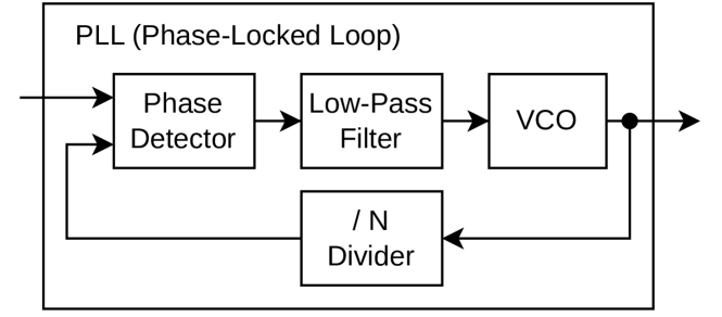
Figure 4: A single loop of PLL.

The low-pass filter removes the high-frequency noise component of the XO. Thus, at the frequency offsets higher than the cut-off frequency $f_{\mathrm{PLL}}$ the PN is defined by the VCO. At the frequency offsets below $f_{\mathrm{PLL}}$ the LO PN is defined by the PN of the XO (amplified according to (15)) and the PN contribution of the phase detector. The total PN of the LO is

$$S_{\mathrm{LO}}(\delta f)=S_{\mathrm{PLL+VCO}}(\delta f)+\frac{S_{\mathrm{XO}}(\delta f)\cdot f_{c}/f_{\mathrm{XO}}}{\sqrt{1+(\delta f/f_{\mathrm{PLL}})^{2}}},$$ (16)

where $f_{\mathrm{XO}}$ is the original XO frequency.

In our simulation, we take closed-loop performance data of PLL+VCO $S_{\mathrm{PLL+VCO}}(\delta f)$ from the datasheets of the particular integrated circuits (ICs), and use it as the input parameters for our model. This data combines the contributions of the VCO noise and phase detector noise.

III-D Real Devices and Their Performance

In this work, we are interested in oscillators’ stabilities at time scales of the 5G NR protocol: from the duration of an OFDM symbol $T_{\mathrm{OFDM}}=71.4$ $\mu$s to the duration of a frame $T_{\mathrm{c}}=1$ ms. Thus, our region of interest is

$$10\mathrm{~{}Hz}\ll 1/T_{\mathrm{c}}\lesssim\delta f\lesssim 1/T_{\mathrm{OFDM}}\ll 100\mathrm{~{}kHz}.$$ (17)

With (16), we compute the LO phase noises at these frequency offsets for the following devices. The resulting PN figures are given in Table I.

III-D1 NI USRP B200

As an example of a simple SDR, we selected NI USRP B200. It has a local thermal-compensated XO (TCXO) reference which is fed to Analog Devices AD9361 transceiver IC including its own PLL+VCO.

III-D2 NI USRP RIO 2954R

As an example of an advanced SDR, we consider the USRP RIO 2954R which is an SDR based on Ettus X300 series, which includes a clock cleaning and distribution IC with two additional PLL loop stages: one with low-noise voltage controlled XO (LN-VCXO) and the second one with high-frequency low-noise VCO. The latter frequncy is then divided (if required) and used for clocking ADC/DAC and as a reference for Maxim Integrated MAX2871 LO.

To simplify our consideration, we use the free-running performance of the LN-VCXO as the reference XO, and the PN of the MAX2871.

III-D3 Instrumental Grade Transceiver

As a reference, we consider the performance of Texas Instruments LMX2594 high-performance RF synthesizer IC locked to Symmetricom 1000C low noise and high short-term stability oven-controlled XO (OCXO).

$\delta f$	1 Hz	10 Hz	100 Hz	1 kHz	10 kHz	100 kHz	1 MHz	10 MHz
USRP B200	-26.0	-52.0	-76.7	-93.9	-101.8	-102.7	-113.1	-138.1
USRP 2954R	-22.0	-62.0	-89.9	-103.7	-101.0	-106.0	-137.4	-156.0
Instrumental	-76.5	-90.9	-100.1	-106.5	-107.8	-108.0	-134.9	-154.9

TABLE I: Calculated phase noise of the considered devices at different frequncy offsets. Values at offsets from 10 Hz to 100 kHz are used for simulating the cell-free scenario with the considered 5G NR numerology.

IV Numerical results

Aligned with selection of FR1, we consider $M=100$ APs with $L=4$ antennas and $K=40$ UEs in an $0.4\times 0.4$ km² area. Large-scale propagation effects are modeled as

$$\beta_{mk}(d)=\Lambda_{0}+10\eta\log(d/d_{0})+\Lambda_{sh},$$ (18)

where $d$ is the distance between AP $m$ and UE $k$, $\Lambda_{0}=-35.3$ is the PL at reference distance $d_{0}=1$ m, pathloss exponent $\eta=3.76$, and $\Lambda_{sh}$ is lognormally distributed with the standard deviation of $\sigma_{sf}=10$. Moreover, UEs transmit with the same power $p=p_{k}=p_{m}=100$ mW in both uplink training and transmission phases. The thermal noise variance is $\sigma_{N}$= -174 dBm/Hz. Regarding the PN model, we use the same parameters as in [7, 8] and (14) for our time scales of one OFDM symbol $T_{\rm OFDM}$, the obtained variance of the innovation equals $0.23$ (note that [9] used 4 times higher variance resulting in even more severe PN).

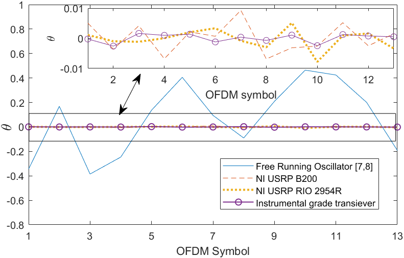
Figure 5: Comparison of the phase drift generated by different models: Realistic LOs are more stable.

Fig. 5 illustrates the difference between PN produced by the model used in [7, 8] and in our study. It is obvious that realistic LOs are substantially more stable than the Free Running Oscillator models used in prior art on CF. Realistic LOs drift moderately resulting in very small CPE while the previously used model produced PN causing significant CPE and ICI effects [9].

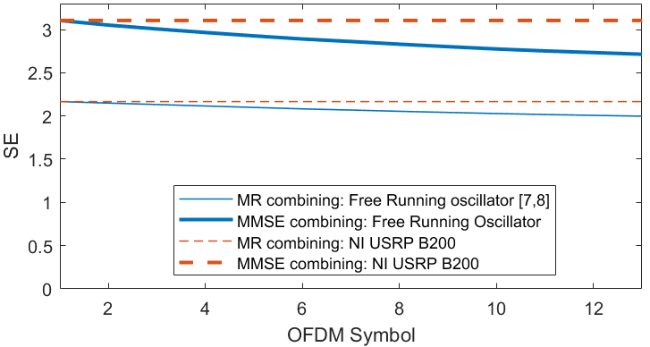
Figure 6: Average SE for different LOs: PN of the realistic LO does not cause performance degradation.

Fig. 6 shows the variation of the achievable SE per user over OFDM symbols due to the evolving CPE. Under severe PN generated by models parameterized as in [7, 8], the achievable SE decreases within one TTI since the aggregate contribution from PN becomes higher. However, when the realistic PN model is used (we use the model of NI USRP B200 as it has the least stable LO), we observe no SE degradation within the TTI (1 ms).

V Conclusions

This study critically examined the performance of Cell-Free (CF) networks under the influence of Phase Noise (PN) using a realistic hardware-based model. Unlike previous works that employed simplified oscillator models, our approach leverages a more accurate representation of Local Oscillators (LO) used in radios like NI USRP B200 and NI USRP RIO. Our findings reveal that even less stable, cost-effective LOs maintain sufficient phase stability to prevent Spectral Efficiency (SE) losses over the standardized 3GPP Transmission Time Interval (TTI) of 1 ms. This substantiates the viability of employing existing 5G standards in the deployment of scalable CF networks for future 6G infrastructure. Furthermore, the resilience of CF networks to hardware imperfections, as demonstrated by our simulations, supports the practical implementation of these networks, potentially alleviating some of the concerns raised by previous theoretical studies.

References

- [1] I. F. Akyildiz, A. Kak, and S. Nie, “6G and Beyond: The Future of Wireless Communications Systems,” IEEE Access, vol. 8, pp. 133 995–134 030, 2020.
- [2] M. Giordani, M. Polese, M. Mezzavilla, S. Rangan, and M. Zorzi, “Toward 6G Networks: Use Cases and Technologies,” IEEE Communications Magazine, vol. 58, no. 3, pp. 55–61, 2020.
- [3] H. Q. Ngo, A. Ashikhmin, H. Yang, E. G. Larsson, and T. L. Marzetta, “Cell-Free Massive MIMO Versus Small Cells,” IEEE Transactions on Wireless Communications, vol. 16, no. 3, pp. 1834–1850, 2017.
- [4] E. Björnson and L. Sanguinetti, “Scalable Cell-Free Massive MIMO Systems,” IEEE Transactions on Communications, vol. 68, no. 7, pp. 4247–4261, 2020.
- [5] D. Wang, C. Zhang, Y. Du, J. Zhao, M. Jiang, and X. You, “Implementation of a Cloud-Based Cell-Free Distributed Massive MIMO System,” IEEE Communications Magazine, vol. 58, no. 8, pp. 61–67, 2020.
- [6] V. Ranjbar, A. Girycki, M. A. Rahman, S. Pollin, M. Moonen, and E. Vinogradov, “Cell-Free mMIMO Support in the O-RAN Architecture: A PHY Layer Perspective for 5G and Beyond Networks,” IEEE Communications Standards Magazine, vol. 6, no. 1, pp. 28–34, 2022.
- [7] A. Papazafeiropoulos, E. Björnson, P. Kourtessis, S. Chatzinotas, and J. M. Senior, “Scalable Cell-Free Massive MIMO Systems: Impact of Hardware Impairments,” IEEE Transactions on Vehicular Technology, vol. 70, no. 10, pp. 9701–9715, 2021.
- [8] Y. Fang, L. Qiu, X. Liang, and C. Ren, “Cell-Free Massive MIMO Systems With Oscillator Phase Noise: Performance Analysis and Power Control,” IEEE Transactions on Vehicular Technology, vol. 70, no. 10, pp. 10 048–10 064, 2021.
- [9] Y. Wu, L. Sanguinetti, U. Gustavsson, A. G. Amat, and H. Wymeersch, “Impact of Phase Noise on Uplink Cell-Free Massive MIMO OFDM,” in IEEE Global Communications Conference, 2023, pp. 5829–5834.
- [10] D. Petrovic, W. Rave, and G. Fettweis, “Effects of Phase Noise on OFDM Systems With and Without PLL: Characterization and Compensation,” IEEE Transactions on Communications, vol. 55, no. 8, pp. 1607–1616, 2007.
- [11] J. Vardakas, M. A. Rahman, E. Vinogradov, S. Barrachina, S. Pryor, W. Van Thillo, P. Chanclou, and D. Kritharidis, “Deliverable D2.2 MARSAL’s network architecture specifications,” Horizon project MARSAL (No 101017171), 2022.
- [12] J. S. Vardakas, K. Ramantas, E. Datsika, M. Payaró, S. Pollin, E. Vinogradov, M. Varvarigos, P. Kokkinos, R. González-Sánchez, J. J. V. Olmos, I. Chochliouros, P. Chanclou, P. Samarati, A. Flizikowski, M. A. Rahman, and C. Verikoukis, “Towards Machine-Learning-Based 5G and Beyond Intelligent Networks: The MARSAL Project Vision,” in 2021 IEEE International Mediterranean Conference on Communications and Networking (MeditCom), 2021, pp. 488–493.
- [13] J. S. Vardakas, K. Ramantas, E. Vinogradov, M. A. Rahman, A. Girycki, S. Pollin, S. Pryor, P. Chanclou, and C. Verikoukis, “Machine Learning-Based Cell-Free Support in the O-RAN Architecture: An Innovative Converged Optical-Wireless Solution Toward 6G Networks,” IEEE Wireless Communications, vol. 29, no. 5, pp. 20–26, 2022.
- [14] R. Beerten, V. Ranjbar, A. P. Guevara, and S. Pollin, “Cell-Free Massive MIMO in the O-RAN Architecture: Cluster and Handover Strategies,” in IEEE Global Communications Conference, 2023, pp. 5943–5948.
- [15] A. Girycki, M. A. Rahman, E. Vinogradov, and S. Pollin, “Learning-based Precoding-aware Radio Resource Scheduling for Cell-free mMIMO Networks,” IEEE Transactions on Wireless Communications, pp. 1–1, 2023.
- [16] M. Chung, L. Liu, and O. Edfors, “Phase-Noise Compensation for OFDM Systems Exploiting Coherence Bandwidth: Modeling, Algorithms, and Analysis,” IEEE Transactions on Wireless Communications, vol. 21, no. 5, pp. 3040–3056, 2022.
- [17] F. Ramian, “Time domain oscillator stability measurement: Allan variance,” Rohde&Schwarz Application Note, Apr. 2015.