Binarized Simplicial Convolutional Neural Networks
Abstract
Graph Neural Networks have a limitation of solely processing features on graph nodes, neglecting data on high-dimensional structures such as edges and triangles. Simplicial Convolutional Neural Networks (SCNN) represent higher-order structures using simplicial complexes to break this limitation albeit still lacking time efficiency. In this paper, we propose a novel neural network architecture on simplicial complexes named Binarized Simplicial Convolutional Neural Networks (Bi-SCNN) based on the combination of simplicial convolution with a binary-sign forward propagation strategy. The usage of the Hodge Laplacian on a binary-sign forward propagation enables Bi-SCNN to efficiently and effectively represent simplicial features that have higher-order structures than traditional graph node representations. Compared to the previous Simplicial Convolutional Neural Networks, the reduced model complexity of Bi-SCNN shortens the execution time without sacrificing the prediction performance and is less prone to the over-smoothing effect. Experimenting with real-world citation and ocean-drifter data confirmed that our proposed Bi-SCNN is efficient and accurate.
keywords:
Graph Learning; Graph Neural Networks; Simplicial Complex; Convolutional Neural Networks1 Introduction
Graphs and networks are gaining enormous awareness in the field of machine learning and artificial intelligence owing to their ability to effectively learn and represent irregular data interactions [1, 2, 3]. Graph structures can be deduced from various real-life applications by embedding the features onto the nodes of graph representations using the graph Laplacian. Sensor graphs of nationwide temperature [4] and air quality [5] are built by combining sensor readings with the sensor location; citation graphs [6] can be formed by linking the citation relationship between authors. In the past, spatial and spectral graph neural networks (GNNs) such as the Graph Convolutional Networks (GCN) [7, 8], Graph Attention Networks (GAT) [9], Graph SAGE [10] and their variants have had major success on graph representation learning tasks including node classification, graph classification, and link prediction. The GCN and the GAT can be generalized by the Message Passing Neural Networks where instead of Global level graph representation done by the graph Laplacian matrix or the graph Adjacency matrix, a localized message-passing scheme is defined for each node [11]. However, GNNs operate only on the features residing on the graph nodes and have not given enough attention to the graph edges and the structures formed by the edges. In the real world, the fact is that data or features can appear not only on the graph nodes but also on higher-order structures. Traffic flow could be recorded on either the edges [12] or the nodes [13] of a graph. A map of ocean drifter trajectories can be modeled using the data on graph edges [14]. In a citation complex, a collaboration among three or even more authors is modeled using simplicial complexes, which is a scenario that cannot be simply recorded using the graph nodes only because a traditional representation of an edge connection between two nodes can only represent a one-to-one relationship between two authors [15]. More such examples where data appears on structures with higher-order than graph nodes include pandemic prediction based on population mobility among regions [16] and dynamic gene interaction graphs [17].
Recently the concept of Topological Signal Processing was introduced: instead of the graph Laplacian, a more generalized Laplacian known as the Hodge Laplacian is adopted in Topological Signal Processing to incorporate the representation of higher-order features that are beyond the graph nodes [18]. In Topological Signal Processing, operations such as spectral filtering, spatial diffusion, and convolution are defined on simplicial complexes using the Hodge Laplacians [19]. High-dimensional feature representations such as data on the graph edges and data on the triangles formed by three edges can be embedded into simplicial complexes using methodologies analogous to graph (node) embedding [20].
If we feed the outputs of the Topological Signal Processing into non-linear active functions the concatenate a few of these together, we can transform them into neural networks. The Simplicial Neural Network (SNN) generalized the GCN onto simplicial complexes by using Topological Signal Processing to extend the convolutional ability of GCN to process higher-order simplicial features [15]. The Simplicial Convolutional Neural Networks (SCNN) [21] further improves the performance of SNN by applying the Hodge decomposition to the simplicial convolution so it is able to train the upper and lower simplicial adjacencies separately. The Simplicial Attention Network (SAT) [22] and the Simplicial Attention Neural Network [23] introduced the attention mechanism to SNN and SCNN to process simplicial features, making them generalized versions of the GAT from graphs to simplicial complexes. The Simplicial Message Passing Networks have generalized the message passing on graphs [11] to simplicial complexes [24]. The Dist2Cycle was proposed to use Simplicial complexes to define neural networks for Homology Localization [25]. These architectures have shown to be successful at applications such as imputing missing data on the citation complexes of different data dimensions and classifying different types of ocean drifter trajectories.
Although the simplicial complex-based neural networks have achieved numerous successes, the focus of the previous networks was on how to extend concepts such as convolution or attention from graphs onto simplicial complexes, which leads to two drawbacks. First, the recently proposed simplicial neural network structures do not prioritize time efficiency, resulting in inefficiency in terms of computational complexity and run time. Let us look into the GCN, which is the 0-simplex analogy of the SNN, the Simplified GCN [26] has proved a trained GCN essentially is a low-pass filter in the spectral domain and the complexity of GCN can be reduced by eliminating nonlinearities and collapsing weights. The Binary-GCN (Bi-GCN) [27] was inspired by the Binary Neural Networks to use binary operations such as XOR and bit count to speed up training time. In the field of Graph Signal Processing, the Adaptive Graph-Sign algorithm derived from -optimization results in a simple yet effective adaptive sign-error update that has outstanding run speed and robustness [28, 29]. To the best of our knowledge, similar improvements that focus on the efficiency and complexity of neural network algorithms on the simplicial complex are absent. Following the first drawback of the current neural network algorithms on simplicial complexes, the high complexity of current simplicial neural network structures may cause the resulting simplicial embeddings to get over-smoothed in some scenarios. In their graph predecessors, the over-smoothed phenomenon was extensively analyzed [30, 31] but has not yet gained enough attention in the simplicial complex-based neural networks.
In this paper, we propose a novel neural network architecture on simplicial complexes named Binarized Simplicial Convolutional Neural Networks (Bi-SCNN) with the following advantages:
-
1.
The Topological Signal Processing foundation of the Bi-SCNN enables Bi-SCNN to process data that have higher-order structures than graph nodes, allowing the Bi-SCNN to effectively represent simplicial data features.
-
2.
The Bi-SCNN can be interpreted using spatial and spectral filters defined using the Topological Signal Processing backbone.
-
3.
The combination of simplicial convolution with a binary-sign forward propagation strategy significantly reduces the model complexity, leading to a reduced training time when compared to existing algorithms such as SCNN, without sacrificing the prediction accuracy. Additionally, the formulation of the Sign() function in the binary-sign forward propagation makes it naturally an activation function.
-
4.
Bi-SCNN is less prone to over-smoothing as a result of the reduced architectural complexity.
2 Related Works
Algorithms that conduct convolution on the nodes of a graph such as GCN [8] operate only on the graph nodes, but not on -simplexes with . Both the SNN [15] and the SCNN [21] are direct extensions of the GCN onto simplicial complexes; SNN is architecturally identical to the SCNN except SNN does not use Hodge decomposition. The Bi-SCNN is an extension of the SCNN [21], but the Bi-SCNN uses feature normalization and feature binarization which the SCNN does not. Also, the binary-sign forward propagation strategy in the Bi-SCNN layer has 2 outputs but the SCNN layer only has 1 output, making a neural network that contains more than 2 layers of Bi-SCNN a drastically different architecture than using purely SCNN.
The Bi-GCN [27] has an acronym similar to the Bi-SCNN, but we should emphasize that the Bi-SCNN is not simply a simplicial complex version of the Bi-GCN and the two are drastically different from each other with the following four differences. Firstly, the Bi-GCN operates only on the graph nodes, while the Bi-SCNN operates on -simplexes. Secondly, as explained earlier, the Bi-SCNN does not follow the traditional GCN/SCNN forward propagation strategy because the feature binarization and the feature normalization propagate separately. Thirdly, the Bi-GCN binarizes both the feature and the trainable weights but Bi-SCNN only binarizes the features. Fourthly, the Bi-GCN uses binary operations bit count and XOR to speed up the same GCN forward propagation and uses predefined values to deal with the backpropagation of binary operations; the Bi-SCNN uses a binary-sign forward propagation and we do not make any predefinitions for backpropagation.
3 Background
We will begin with a set of vertex to define a -simplex , where is a subset of with cardinality . Throughout the paper, subscript is used to denote which a variable belongs to. The collection of -simplexes with is a simplicial complex of order . If generalizing a graph as a simplicial complex, the vertex set of is the node set that belongs to and the edge set belongs to . Note that for a simplex , if is a subset of , then . We use the variable to denote the number of elements of . Take a graph as an example, is the number of nodes and is the number of edges. Each simplicial feature vector of a simplex is a mapping from the -simplex to and will be denoted as [18] . Simplicial data with features will be denoted as = [].
To process the data on a simplicial complex, we will be using the Hodge Laplacian matrix defined as follows:
| (1) |
where the is the incidence matrix that represents the relationship between adjacent simplices and in . Each row of correspond to one element in , and each column of correspond to one element in . Each adjacency relationship between and will result in a entry in with the sign determined by the orientation of the element in . One useful property of the incidence matrix is .
One can see an important characteristic of , for , can be split into and (1); is the lower Hodge Laplacian that represents the lower adjacencies of , and is the upper Hodge Laplacian that represents the upper-adjacency of [18]. It is worth pointing out an important property of the SFT in the spectral domain: the eigenvectors paired with the non-zero eigenvalues of are orthogonal to the eigenvectors paired with the non-zero eigenvalues of [18].
The graph Laplacian matrix seen in GCN or GAT is . Two examples of incidence matrices are and , which are the node-to-edge incidence matrix and the edge-to-triangle incidence matrix respectively.
4 Derivations of the Binarized Simplicial Convolutional Neural Networks
We will begin with the simplicial convolution on a -simplex, which is the theoretical foundation of our Bi-SCNN, along with a discussion of spectral and spatial Topological Signal Processing techniques. Then, we will provide the derivations of Bi-SCNN and combine binary-sign updates, simplicial filters, and nonlinearities to form our Bi-SCNN layer. The goal is to improve the simplicial convolution shown in (7) by reducing its computational complexity and making it less prone to over-smoothing.
4.1 Simplicial Convolution
In GNNs, operations such as graph convolution and embedding of the node features are possible by the computations defined by the graph Laplacian. For instance, the spatial graph convolution in GCN aggregates the data from the 1-hop neighbors of each node by [8]. Graph convolution can also be defined by applying low-pass filters in the spectral domain to data on the graph nodes [7].
In Topological Signal Processing, an equivalent analogy can be drawn by defining spatial and spectral operations using the Hodge Laplacian. The convolution is essentially transforming spatial data into the spectral domain, applying a filter in the spectral domain to the simplicial data, and using the inverse transform to transform the filtered data back into the spatial domain [18]. For a set of features to be able to transform between domains in a -simplex, we need the simplicial Fourier transform (SFT) defined by the eigendecomposition of the Hodge Laplacian matrix. For the -simplex, the SFT is the eigendecomposition
| (2) |
where is the eigenvector matrix and is the eigenvalue matrix. The eigenvalues on the diagonals of are arranged in increasing order and are referred to as frequencies and each eigenvector is the column of appearing in the same order. The forward SFT is , and the inverse SFT is respectively. A simplicial filter can be represented using a function on the frequencies matrix . The output of a spectral simplicial convolution when the input is a one-dimensional simplicial vector :
| (3) |
The spectral convolution of a -simplex with feature size relies on the eigendecomposition that has complexity and is numerically unstable when is large. Luckily, it has been shown that a series of polynomial summations approximate the above spectral approach, resulting in the spatial simplicial convolution [19]:
| (4) |
where is the filter weight and the is the filter length of the spatial Simplicial Convolution.
Let us introduce another concept named the Hodge decomposition before we proceed to the Simplicial Convolution:
| (5) |
where is the portion of that is induced from , is the portion of that is induced from , and is the harmonic component that cannot be induced [18]. The harmonic component of has the property of
| (6) |
In other words, the Hodge decomposition essentially decomposes the Hodge Laplacian matrix into the gradient, curl, and harmonic components [19].
In (4), we can assign specific filter weights to the lower and upper Hodge Laplacians because by definition, in (1), the Hodge Laplacian matrix can be split into the upper and the lower Laplacian. This leads to the (single feature) convolution operation seen in SCNN [21]:
| (7) |
where is the weights of the lower Hodge Laplacian and is the weights for the upper Hodge Laplacian. A term is added to the simplicial convolution because of the property shown in (6): the role of is to take into account of the harmonic component as it can only be processed independently from the upper or lower Laplacian [18]. Combining the simplicial convolution with nonlinearity, the forward propagation of an SCNN layer is
| (8) |
where is the activation function, is the layer number, and is the output of the simplicial layer [21]. In the SCNN, , , and are the trainable weights to be optimized. Each -simplex in a simplicial complex with order will have individually their own -simplex SCNN.
To facilitate later derivations, we will provide the expression for the multi-variate version of the simplicial convolution in (7) when there are features in the data :
| (9) |
where , , and are the trainable weights with their sizes determined by the number of input and output features of layer . The SCNN multi-variate version of the SCNN is also provided here as it was not given in the SCNN original literature [21]:
| (10) |
In the first layer, the input is . We will refer to the above spatial simplicial convolution as the simplicial convolution throughout the rest of the paper.
4.2 Over-Smoothing Alleviation via Architectural Simplifications
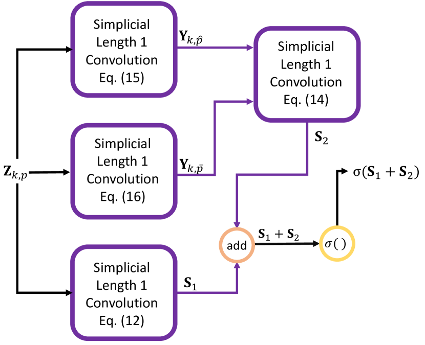
First, notice that for , we can intuitively acquire each summation term of length convolution by feeding our input into a series of concatenated length 1 convolution. In other words, one SCNN layer of length is equivalent to combining many SCNN layers of length without nonlinearity. To see this more clearly, let us consider the case of and break down (10):
| (11) |
where
| (12) |
and
| (13) |
It is easy to see that is just a length 1 convolution if we set in (9). Now, as with , it actually can be formulated as
| (14) |
where
| (15) |
and
| (16) |
From the above equations, it is not difficult to check that for one SCNN layer with , it is equivalent to having a combination of SCNN layers with stacked in two layers; a visualization of breaking down (11) is provided in Figure 1.
In order to avoid this complexity of SCNN, our Bi-SCNN will be formed using purely length 1 simplicial convolution which gives us the advantage of alleviating over-smoothing. Let us look at the cause of over-smoothing. Each multiplication of the Hodge Laplacian is a 1-hop neighbor aggregation because, by definition, the non-diagonal elements of the Hodge Laplacian matrix are non-zero only when there is a neighbor in between and two elements and . So, multiplying the Hodge Laplacian with a feature vector essentially aggregates all the neighborhood features that are 1-hop away, and doing it for will aggregate from -hops away. For the SCNN layer in (8), if is large enough, one single SCNN layer is possible to aggregate the entire simplex as each will aggregate from neighbors further and further. The over-smoothing problem is the exact analogy of what was seen in the GCNs [31] where the over-smoothed output has similar values among different elements in a simplex and causes the output to be indistinguishable. In the past, one simple yet effective solution to this problem on the graph neural network algorithms was to reduce the number of layers. In Bi-SCNN, we set the length of the filter to , and treat the number of layers as a hyperparameter during training to reduce over-smoothing.
4.3 Computational Complexity Reduction via Binarization of Simplicial Features
Let us now examine how to enhance the time efficiency of simplicial convolution while maintaining the effectiveness of its simplicial embedding. One of the many solutions to this is the Binarization similar to what is seen in the Bi-GCN [27], where both the trainable weights and the features are binarized and the forward propagation is done by binary operations bit count and XOR to combine the binarized weights and features into a new node embedding. Another approach is seen in the Graph-Sign algorithms [28], which delivers a sign-error update at each iteration that has a low run time and a low complexity. Aside from the fact that these node-based algorithms are not suitable to be deployed on simplicial complexes, there are a few additional problems to be addressed. The Bi-GCN binarizes both the weights and features, leading to reduced performance under certain circumstances. Also, even though Bi-GCN uses binary operations to optimize the computation cost, the forward propagation is indifferent and mathematically identical compared with the original GCN. The Graph-Sign algorithm operates on a predefined bandlimited filter, which may require prior expert knowledge to obtain.
We propose a new forward propagation strategy where we combine feature normalization, feature binarization, and binary-sign propagation together to form a fast and accurate Binarized Simplicial Convolution. Let us first begin with the multi-variate simplicial convolution in (10). Following the graph-based feature binarization seen in Bi-GCN [27], we define the feature binarization of simplicial data on -simplex as
| (17) |
where is the Hadamard product, Sign is the Sign function and is the (weighted) binarized simplicial features. The matrix acts as the weights for the binarized features and is formed by a feature normalization:
| (18) |
where is the -norm done on the row of ( in (18)) and is the number of features in . All elements of the same row in have the same value, but this is only for mathematical representation convenience. In practice, is stored as a vector and is broadcasted using element-wise multiplications when used to multiply with . Notice that the Sign() function only outputs binary values and assuming that we ignore the zeros, this means that the size of the binarized features is reduced in practice when compared to [27].
Now, plugging the feature binarization (17) into (10) and setting , we will get
| (19) |
Looking at the expression in (19), aside from benefiting from the model size reduction, it still follows the exact same forward propagation strategy as SCNN, making it have roughly the same time to execute in practice. We would like to further improve the run speed of this Binary setup by propagating only the Sign() part. Using the two properties of Hadamard products and , with some algebraic derivations, equation (19) becomes
| (20) |
Notice that the -norm is nonnegative, so at each layer, can be viewed as ReLu(). The input of the layer in (20) will binarize the output of the layer regardless of the magnitude, so we can safely input only the binarized simplicial features (without the weights ) to the layer when . Also, we should point out that the Sign() function is non-linear. In this way, the nonlinearity in both the Sign() function and the -norm can serve as activations in forward propagation. The forward propagation of a series of concatenated Bi-SCNN is obtained by rearranging (20) a using the property again:
| (21) |
where for the layer
| (22) |
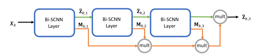
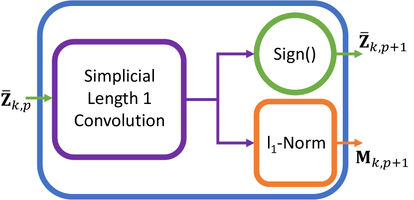
Even though the Sign() function has no derivative at 0 due to its discontinuity at and a derivative of for all other values, we approximate Sign() using a hard tanh function, allowing us to conduct forward propagation and backward propagation as usual. The way to achieve the forward propagation in (21) in practice is that each Bi-SCNN layer will have two outputs: the feature normalization and feature binarization . Notice that only will be forward-propagated to the next Bi-SCNN layer, meaning that . Exceptions are: at the first layer where is the input, and the final layer all the are multiplied together at the end to form . An illustration of a Bi-SCNN network with is shown in Fig. 2.
Intuitively, a single Bi-SCNN layer on a -simplex can be understood as using the (upper and lower) Hodge Laplacians to aggregate the weighted simplicial features with the addition of the harmonic component. From the spatial Topological Signal Processing perspective, the weights are trained to optimize a binary-sign feature aggregation with a matrix that records the magnitude of each aggregation. From the spectral Topological Signal Processing perspective, the goal of training a Bi-SCNN is to obtain a filter for the binary-sign update that best fits the spectrum of the training data. An illustration of one Bi-SCNN layer can be found in Fig. 2.
Aside from the fact that all algorithms benefit from the sparsity of , let us look into (21) to see the high time-efficiency of Bi-SCNN. In practice, Sign() is approximated by Hardtanh(), meaning that a percentage of the matrix consists only of s and s. In this case, element-wise multiplications can be omitted in the matrix multiplication, reducing multiplications to multiplications. Assuming each multiplication is 1 FLOP, each Bi-SCNN layer is at least FLOPS faster than the SCNN layer for the layer and beyond. Also, in the actual implementation of SCNN, to compute , , , and are concatenated into a matrix for each ; then matrices are stacked into a tensor. Trainable weights , , and are stacked into a tensor in a similar manner. Afterward, is computed by the Einstein summation between two tensors (aggregation and weight tensors) of size and back into a matrix of size . This matrix concatenation, stacking, and Einstein summation approach of the SCNN is less time efficient than direct matrix multiplication in Bi-SCNN considering we are using binarized features, especially when . We should emphasize again that is a broadcasted vector in practice, making the Bi-SCNN more efficient.
5 Experiment Results and Discussion
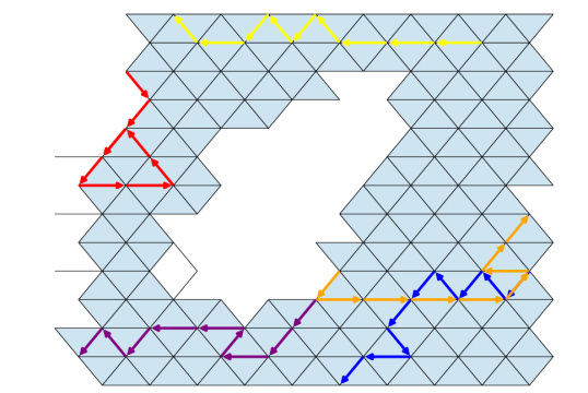
The Citation Complex [15] and the Ocean Drifter Complex [14] are chosen because both datasets are already preprocessed to have features defined in simplexes with order , making them suitable choices to test the performance of an algorithm on simplicial complexes. We would like to verify that the Bi-SCNN has a faster execution time while maintaining good accuracy when compared against existing simplicial algorithms. The experiments are conducted on one Nvidia RTX 3090 GPU with PyTorch version 1.8.0 and CUDA version 11.1. None of the two datasets provided a validation set so the experiments are tuned based on the training performance. All the experiments were repeated 10 times; we calculated the mean and standard derivation of the metrics. A visualization of the ocean drifter complex with illustrations of 5 different ocean drifter trajectories is shown in Figure 4.
| SNN-2 | SCNN-2 | SCNN-3 | Bi-SCNN-3 | Bi-SCNN-2 | |
| 10 missing | |||||
| 90.6003.47 | 90.510.34 | 90.570.38 | 84.5217.95 | 90.650.32 | |
| 91.0002.45 | 91.020.25 | 90.521.43 | 90.770.24 | 91.030.24 | |
| 90.9405.59 | 90.600.67 | 91.220.16 | 87.8101.91 | 91.220.16 | |
| 91.4503828 | 91.370.14 | 91.580.12 | 89.7401.65 | 91.580.12 | |
| 87.8911.59 | 91.650.56 | 91.880.23 | 85.0416.80 | 91.920.20 | |
| 83.6118.65 | 92.070.33 | 82.9627.64 | 89.440.49 | 92.210.23 | |
| 20 missing | |||||
| 81.220.63 | 81.360.64 | 81.140.63 | 81.080.61 | 81.390.66 | |
| 82.170.32 | 82.160.32 | 69.7626.24 | 82.070.25 | 82.200.31 | |
| 82.420.49 | 82.260.51 | 74.4224.81 | 80.530.58 | 82.680.27 | |
| 83.110.38 | 82.970.26 | 83.230.15 | 81.811.28 | 83.230.15 | |
| 75.6323.65 | 83.470.40 | 81.845.39 | 82.790.45 | 83.640.19 | |
| 73.0325.38 | 84.220.27 | 75.8825.30 | 66.452.69 | 84.340.23 | |
| 30 missing | |||||
| 72.160.66 | 72.270.57 | 71.821.28 | 72.050.61 | 72.330.50 | |
| 73.150.42 | 73.130.44 | 72.870.52 | 72.640.79 | 73.980.41 | |
| 73.730.67 | 73.460.51 | 66.7021.96 | 72.200.32 | 73.980.26 | |
| 74.700.30 | 74.520.21 | 67.2922.43 | 72.440.40 | 74.780.16 | |
| 68.3121.98 | 75.560.26 | 68.0522.69 | 74.7308.27 | 75.680.20 | |
| 72.0910.87 | 76.520.31 | 76.630.24 | 65.0018.89 | 76.630.23 | |
| 40 missing | |||||
| 62.360.72 | 62.780.65 | 62.071.83 | 62.590.61 | 62.810.65 | |
| 64.100.28 | 64.100.28 | 63.740.91 | 63.570.79 | 64.100.28 | |
| 64.730.79 | 64.540.63 | 65.520.20 | 63.860.32 | 65.170.20 | |
| 66.260.28 | 66.070.33 | 66.310.21 | 65.400.40 | 66.310.21 | |
| 66.891.66 | 67.330.39 | 50.2627.14 | 66.850.83 | 67.570.23 | |
| 61.9814.03 | 68.860.18 | 62.2120.31 | 53.9118.89 | 68.980.18 | |
| 50 missing | |||||
| 54.010.5457 | 54.030.06 | 53.980.58 | 50.285.35 | 54.180.52 | |
| 55.050.3947 | 55.080.04 | 54.331.37 | 54.210.94 | 55.810.40 | |
| 55.322.1300 | 55.780.06 | 56.270.24 | 52.954.04 | 56.270.24 | |
| 57.810.3062 | 57.330.03 | 57.820.28 | 57.190.37 | 57.850.25 | |
| 57.644.4258 | 59.050.04 | 59.540.29 | 57.983.21 | 59.540.29 | |
| 49.8716.5068 | 60.720.09 | 61.150.19 | 55.396.39 | 61.150.19 | |
| SNN-2 | SCNN-2 | SCNN-3 | Bi-SCNN-3 | Bi-SCNN-2 | |
|---|---|---|---|---|---|
| 10 missing | 1410.37 s | 3652.23 s | 92711.58 s | 350.18 s | 21 0.78 s |
| 20 missing | 1300.19 s | 3561.87 s | 9458.42 s | 360.20 s | 22 1.73 s |
| 30 missing | 1240.61 s | 3583.11 s | 9579.04 s | 360.20 s | 22 1.35 s |
| 40 missing | 1240.41 s | 3622.78 s | 8929.86 s | 350.24 s | 22 1.12 s |
| 50 missing | 1240.22 s | 3572.80 s | 9315.71 s | 360.24 s | 22 1.18 s |
5.1 Citation Complex
The raw data of the Citation Complex is from Semantic Scholar Open Research Corpus [32], where the number of citations of authors forms a -simplex where . The 6 simplices naturally form a simplicial complex because they form a hierarchical structure: each -simplex is a subset author collaborations of the -simplex. To examine the performance of our Bi-SCNN algorithm, we will follow the training and testing procedure seen in SNN [15] and SCNN [21]. For each -simplex a portion of the simplicial data will be missing at random. In this transductive learning task, the goal is to impute the missing data from the existing data. We will be testing 5 different missing rates: 10%, 20%, 30%, 40%, and 50%.
A 2-layer Bi-SCNN (Bi-SCNN-2) and a 3-layer Bi-SCNN (Bi-SCNN-3) will be compared against a 2-layer SNN (SNN-2), a 2-layer SCNN (SCNN-2), and a 3-layer SCNN (SCNN-3). The number of simplicial filters per layer is set to 30 for all algorithms. Each layer in SNN-2 and SCNN-2 will have a length to keep the model size roughly the same order of magnitude as the Bi-SCNN-2. SCNN-3 will have a filter length , which is the best-performing setting seen in the original paper [21]. GCN is not included because SNN is equivalent to the GCN for .
We follow the parameter optimization seen in SCNN [21] where all algorithms use Adam optimizer with a learning rate of and minimize the -loss on the training set for 1000 iterations. To make the comparison fair, all the tested algorithms use purely Simplicial Layers except for the activation functions. The accuracy of the imputed missing data will be considered as correct if it is within of the ground truth value. The experiment run time is recorded on the total run time of all the forward and backward propagation. The accuracy of each algorithm setting is shown in Table 1. The run time of the experiments is recorded in Table 2; there is also a visual illustration of the run time for 10 missing rate in Figure 5. A summary of the number of trainable parameters of each algorithm can be found in Table 5. The mean training loss of the 10 experiment runs of all the tested algorithms on the Citation Complex with missing data is shown in Fig. 6.
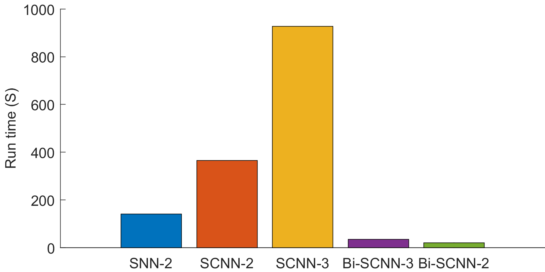
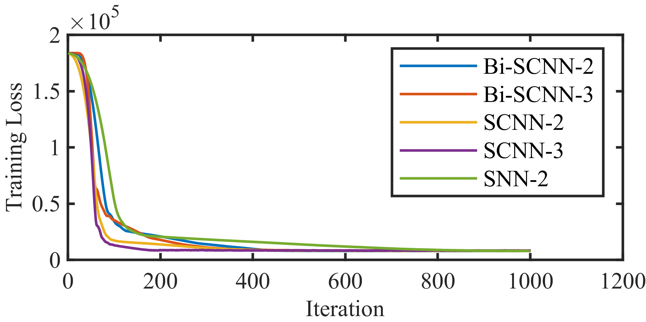
Looking at Figure 6, we can see that all the tested algorithms converge and their convergence behaviors are distinctively different. The different convergence behavior is an indication of them having different simplicial representations. From Table 1, we can see that 2-layer Bi-SCNN performs the best in most of the simplices under all the tested missing rates. This confirms that even though the Bi-SCNN uses a simpler propagation scheme by only having a length-1 simplicial filter, the embedding power is equivalent to the SNN or SCNN in the current experiment. Another interesting observation is that the 2-layer models perform slightly better than the 3-layer models in many cases. We think this is due to the fact that the 3-layer models have too many simplicial convolutional filters and the simplicial embedding got over-smoothed during the propagation process. If we look at the ratio of parameter size to run time, we can see that the Bi-SCNN is the most efficient among all the tested algorithms. Bi-SCNN-2 has 20% more parameters than SNN-2 but takes only the time that SNN needs to complete the experiment. We should point out that for roughly similar model sizes, the Bi-SCNN has higher accuracy in imputing the citations compared to the SNN because Bi-SCNN uses assigns weights separately by considering upper and lower simplicial adjacencies separately but SNN does not, making the Bi-SCNN more expressive. The Bi-SCNN is indeed a more concise model than the SNN and the SCNN because not only does Bi-SCNN use fewer parameters but also operates faster. The reason that the Bi-SCNN is time-efficient is that the binary-sign propagation takes fewer computations, which is proven in traditional CNN [33] and has also been proven when data is purely on the nodes of the graph by the G-Sign [28] and Bi-GCN [27]. We can conclude that the Bi-SCNN can effectively and efficiently impute the missing citations compared to the SCNN and SAT.
| SAT | SCNN | Bi-SCNN | |
|---|---|---|---|
| Id, 2 | 60.256.47 | 64.003.39 | 71.254.0 |
| Id, 3 | 64.755.30 | 69.002.78 | 71.00 4.06 |
| LR, 2 | 61.757.24 | 77.004.00 | 79.503.67 |
| LR, 3 | 62.252.08 | 81.752.97 | 77.004.15 |
| Tanh, 2 | 64.006.04 | 74.756.75 | 78.755.94 |
| Tanh, 3 | 66.55.50 | 75.256.66 | 73.753.01 |
| SAT | SCNN | Bi-SCNN | |
|---|---|---|---|
| Id, 2 | 1196 s | 2197 s | 143 s |
| Id, 3 | 1515 s | 6450 s | 232 s |
| LR, 2 | 1116 s | 2187 s | 165 s |
| LR, 3 | 1385 s | 6441 s | 231 s |
| Tanh, 2 | 1161 s | 2196 s | 150 s |
| Tanh, 3 | 1491 s | 6399 s | 234 s |
5.2 Ocean Drifter Complex
The Ocean Drifter Complex is a dataset formed by using simplicial embedding to represent real-world ocean drifters around Madagascar Island [14]. The ocean that surrounds Madagascar Island is divided into hexagonal grids and each grid is represented by a node in the -simplex. If the trajectory of an ocean drifter passes two adjacent hexagonal grids an edge will be formed between the node. In the dataset, there are two types of trajectories and the goal is to classify which type of trajectory the input trajectory belongs to. A visualization of this dataset is shown in Figure 4. We should emphasize that the formed simplex structure itself is undirected, but the data that resides on the simplex has orientations.
The data provided 160 training trajectories and 40 testing trajectories all on the -simplex. In other words, the feature only exists on the edges. Our baseline algorithms are SAT [22] and SCNN [21]. We will follow the batch training procedure seen in SAT [22] but with the batch size set to 40 and each experiment run consists of 5000 epochs. For all three algorithms, we will be running two different architectural settings: 2 simplicial layers and 3 simplicial layers. As suggested by [22], the simplicial layers are followed by a mean pooling layer, then 2 MLP readout layers, and finally a softmax layer. For each architectural setting, there will be three different choices of activation function: identity (id) function, leaky ReLu (LR) function, and tanh function. The SAT suggests the choices of Id and Tanh functions because odd activation functions lead to orientation-equivariant output, which is shown to perform well on a synthetic ocean drifter dataset [22]. The classification accuracy is shown in Table 3 and the time to complete the experiments is recorded in Table 4. The number of trainable parameters of each setting is shown in Table 5.
In the Ocean Drifter Dataset, we can observe again that the Bi-SCNN has similar classification accuracy as the SCNN for all three choices of action functions. The reason Bi-SCNN is able to consistently outperform SAT is due to the fact that the Bi-SCNN utilizes the Hodge decomposition: Bi-SCNN optimizes parameters for upper and lower adjacencies separately but the SAT uses the standard Hodge Laplacian. Additionally, the processing of the harmonic component of the input simplicial features is absent in SAT, making its simplicial embedding less representative than convolution-based algorithms. One may notice that the run time reduction of Bi-SCNN is not as prominent in the ocean drifter complex as in the citation complex. This is because when we recorded the run time, the global pooling and the 2 MLP layers also contributed to the time in addition to the time it takes to run the simplicial layers. The Bi-SCNN does not optimize the global pooling and the 2 MLP layers, so these layers will perform indifferently among Bi-SCNN, SAT, and SCNN. Still, Bi-SCNN is the fastest among Bi-SCNN, SAT, and SCNN when all three are compared under the same number of simplicial layers.
| Citation | Ocean Drifter | |
| SAT-2 | - | 5762 |
| SAT-3 | - | 6722 |
| SNN-2 | 906 | - |
| SCNN-2 | 1986 | 4712 |
| SCNN-3 | 29166 | 10142 |
| Bi-SCNN-2 | 1146 | 3750 |
| Bi-SCNN-3 | 15726 | 6450 |
6 Conclusion
We introduced Bi-SCNN, combining simplicial convolution with binary-sign propagation. Incorporating the upper and lower adjacencies using the Hodge Laplacian matrix, the Bi-SCNN can effectively capture higher-order structured simplicial features. Bi-SCNN outperforms previously proposed SNN algorithms on citation and ocean drifter complexes in terms of time efficiency, while maintaining comparable prediction accuracy.
References
- [1] A. Ortega, P. Frossard, J. Kovačević, J. M. F. Moura, P. Vandergheynst, Graph signal processing: Overview, challenges, and applications, Proc. IEEE 106 (5) (2018) 808–828.
- [2] D. I. Shuman, S. K. Narang, P. Frossard, A. Ortega, P. Vandergheynst, The emerging field of signal processing on graphs: Extending high-dimensional data analysis to networks and other irregular domains, IEEE Signal Process. Mag. 30 (2013) 83 – 98.
- [3] A. Sandryhaila, J. M. Moura, Big data analysis with signal processing on graphs: Representation and processing of massive data sets with irregular structure, IEEE Signal Process. Mag. 31 (5) (2014) 80 – 90.
- [4] M. J. M. Spelta, W. A. Martins, Normalized lms algorithm and data-selective strategies for adaptive graph signal estimation, Signal Processing 167 (2020) 107326.
- [5] C. Wang, Y. Zhu, T. Zang, H. Liu, J. Yu, Modeling Inter-Station Relationships with Attentive Temporal Graph Convolutional Network for Air Quality Prediction, 2021, p. 616–634.
- [6] A. K. McCallum, K. Nigma, J. Rennie, K. Seymore, Automating the construction of internet portals with machine learning, Information Retrieval 3 (2000) 127–163.
- [7] M. Defferrard, X. Bresson, P. Vandergheynst, Convolutional neural networks on graphs with fast localized spectral filtering, Advances in neural information processing systems 29.
- [8] T. N. Kipf, M. Welling, Semi-supervised classification with graph convolutional networks, arXiv preprint arXiv:1609.02907.
- [9] P. Veličković, G. Cucurull, A. Casanova, A. Romero, P. Lio, Y. Bengio, Graph attention networks, ICLR.
- [10] W. Hamilton, Z. Ying, J. Leskovec, Inductive representation learning on large graphs, Advances in Neural Information Processing Systems 30.
- [11] M. Fey, J. E. Lenssen, Fast graph representation learning with pytorch geometric, in: ICLR, 2019.
- [12] M. T. Schaub, S. Segarra, Flow smoothing and edge denoising: Graph signal processing in the edge space, in: GlobalSIP, 2018, pp. 735–739.
- [13] B. Yu, H. Yin, Z. Zhu, Spatio-temporal graph convolutional networks: A deep learning framework for traffic forecasting, IJCAI.
- [14] M. T. Schaub, A. R. Benson, P. Horn, G. Lippner, A. Jadbabaie, Random walks on simplicial complexes and the normalized hodge 1-laplacian, SIAM Review 62 (2) (2020) 353–391.
- [15] S. Ebli, M. Defferrard, G. Spreemann, Simplicial neural networks, NeurIPS Workshop TDA and Beyond.
- [16] G. Panagopoulos, G. Nikolentzos, M. Vazirgiannis, Transfer graph neural networks for pandemic forecasting, AAAI 35 (6) (2021) 4838–4845.
- [17] S. Ancherbak, E. E. Kuruoglu, M. Vingron, Time-dependent gene network modelling by sequential monte carlo, IEEE/ACM Trans. Comput. Biol. Bioinf. 13 (6) (2016) 1183–1193.
- [18] S. Barbarossa, S. Sardellitti, Topological signal processing over simplicial complexes, IEEE Trans. Signal Process. 68 (2020) 2992–3007.
- [19] M. Yang, E. Isufi, M. T. Schaub, G. Leus, Simplicial convolutional filters, IEEE Trans. Signal Process. 70 (2022) 4633–4648.
- [20] A. Martino, A. Giuliani, A. Rizzi, (hyper) graph embedding and classification via simplicial complexes, Algorithms 12 (11) (2019) 223.
- [21] M. Yang, E. Isufi, G. Leus, Simplicial convolutional neural networks, in: ICASSP, 2022, pp. 8847–8851. doi:10.1109/ICASSP43922.2022.9746017.
- [22] C. W. J. Goh, C. Bodnar, P. Lio, Simplicial attention networks, ICLR Workshop on Geometrical and Topological Representation Learning.
- [23] L. Giusti, C. Battiloro, P. Di Lorenzo, S. Sardellitti, S. Barbarossa, Simplicial attention neural networks (2022).
- [24] C. Bodnar, F. Frasca, Y. Wang, N. Otter, G. F. Montufar, P. Lio, M. Bronstein, Weisfeiler and lehman go topological: Message passing simplicial networks, in: ICML, PMLR, 2021, pp. 1026–1037.
- [25] A. D. Keros, V. Nanda, K. Subr, Dist2cycle: A simplicial neural network for homology localization, in: AAAI, Vol. 36, 2022, pp. 7133–7142.
- [26] F. Wu, A. Souza, T. Zhang, C. Fifty, T. Yu, K. Weinberger, Simplifying graph convolutional networks, in: ICML, Vol. 97 of Proceedings of Machine Learning Research, 2019, pp. 6861–6871.
- [27] J. Wang, Y. Wang, Z. Yang, L. Yang, Y. Guo, Bi-gcn: Binary graph convolutional network, CVPR (2021) 1561–1570.
- [28] Y. Yan, E. E. Kuruoglu, M. A. Altinkaya, Adaptive sign algorithm for graph signal processing, Signal Processing 200 (2022) 108662.
- [29] Y. Yan, E. E. Kuruoglu, Fast and robust wind speed prediction under impulsive noise via adaptive graph-sign diffusion, in: IEEE CAI, 2023, pp. 302–305.
- [30] Q. Li, Z. Han, X.-M. Wu, Deeper insights into graph convolutional networks for semi-supervised learning, in: AAAI, Vol. 32, 2018.
- [31] M. Liu, H. Gao, S. Ji, Towards deeper graph neural networks, in: KDD, 2020, p. 338–348.
- [32] W. Ammar, D. Groeneveld, C. Bhagavatula, I. Beltagy, M. Crawford, D. Downey, J. Dunkelberger, A. Elgohary, S. Feldman, V. Ha, et al., Construction of the literature graph in semantic scholar, Proceedings of the North American Chapter of the Association for Computational Linguistics.
- [33] M. Courbariaux, I. Hubara, D. Soudry, R. El-Yaniv, Y. Bengio, Binarized neural networks: Training deep neural networks with weights and activations constrained to +1 or -1, Algorithms 12(11).