Optimal Group Fair Classifiers from Linear Post-Processing

Abstract

We propose a post-processing algorithm for fair classification that mitigates model bias under a unified family of group fairness criteria covering statistical parity, equal opportunity, and equalized odds, applicable to multi-class problems and both attribute-aware and attribute-blind settings. It achieves fairness by re-calibrating the output score of the given base model with a “fairness cost”—a linear combination of the (predicted) group memberships. Our algorithm is based on a representation result showing that the optimal fair classifier can be expressed as a linear post-processing of the loss function and the group predictor, derived via using these as sufficient statistics to reformulate the fair classification problem as a linear program. The parameters of the post-processor are estimated by solving the empirical LP. Experiments on benchmark datasets show the efficiency and effectiveness of our algorithm at reducing disparity compared to existing algorithms, including in-processing, especially on larger problems.

1 Introduction

Algorithmic fairness has emerged as an important topic in machine learning, amid growing concerns that machine learning models may propagate the bias in past data against historically disadvantaged demographics (Bolukbasi et al., 2016; Buolamwini and Gebru, 2018; Barocas et al., 2023), particularly for models deployed in sensitive domains like criminal justice, healthcare, and finance (Barocas and Selbst, 2016; Berk et al., 2021). Work on this topic are focused on aspects including the evaluation and measurement of model unfairness, the design of fair learning algorithms, and the inherent limitations and trade-offs in achieving fairness (Kleinberg et al., 2017; Zhao and Gordon, 2019). There are fairness metrics that look at model behavior on “similar” individuals called individual fairness (Dwork et al., 2012), and group fairness metrics that consider model output statistics conditioned on each demographic group, such as statistical parity (SP, a.k.a. independence; Calders et al., 2009), equal opportunity (EOpp), equalized odds (EO, separation; Hardt et al., 2016), and predictive parity (sufficiency, or group-wise calibration; Chouldechova, 2017).

Fair learning algorithms, typically designed with specific fairness metrics in mind, can be categorized into pre-processing, in-processing, and post-processing approaches, depending on where bias mitigation takes place in the training pipeline. Pre-processing addresses perhaps the source of unfairness—bias in training data—via data cleaning or reweighting techniques to remove biased correlations (Kamiran and Calders, 2012; Calmon et al., 2017). In-processing algorithms optimize models w.r.t. fairness-constrained objectives (Zemel et al., 2013; Zafar et al., 2017; Agarwal et al., 2018; Zhao et al., 2020). Post-processing algorithms remap the output of pre-trained models to satisfy fairness, and the remapping typically takes much simpler forms than the base model.

Post-processing algorithms are flexible and lightweight. They are model-agnostic and applied post hoc with small computation overhead, hence more appealing than pre-processing and in-processing in scenarios where the criteria for fairness treatment are to be determined after the model is trained and evaluated, or retraining (subject to fairness) is expensive or not possible, e.g., with large foundation models and “model as a service” paradigms (Sun et al., 2022; Gan et al., 2023). Although problem instances can be constructed to make post-processing underperform in-processing under optimization oracles and constrained hypothesis classes that exclude the Bayes optimal predictor (Woodworth et al., 2017), the empirical study of Cruz and Hardt (2024) suggests that these failure cases are rare in real-world data, and post-processing can achieve better accuracy-fairness trade-offs in practice. Theoretically, provided Bayes optimal base model, post-processing is optimal (Theorem 3.3; also see (Chzhen et al., 2020; Le Gouic et al., 2020) for the regression setting).

The limitation of existing post-processing algorithms for fair classification is that they are often stylized to specific fairness criteria and problem settings. The post-processing algorithms of Jiang et al. (2020), Gaucher et al. (2023), Denis et al. (2023), Xian et al. (2023), and Zeng et al. (2024) only support SP. Hardt et al. (2016) and Chzhen et al. (2019) consider EOpp and EO under the attribute-aware setting (i.e., the sensitive attribute is explicitly available when making predictions); attribute-awareness is also required by the algorithms of Menon and Williamson (2018) and Zeng et al. (2022). Alghamdi et al. (2022) and Ţifrea et al. (2024) propose algorithms that project the base model’s output scores to satisfy fairness by minimizing the divergence of the projected scores to the original ones, but this objective may not be aligned with classification metrics such as accuracy. Recently, Chen et al. (2024) proposed a post-processing framework applicable to parity group fairness criteria (covering SP, EOpp, EO) under both attribute-aware and blind settings, but it is limited to binary classification, and requires computationally-intensive optimization procedures.

Contributions.

Continuing the above line of work, we propose a post-processing algorithm for fair classification under parity group fairness criteria (Definition 2.2), applicable to binary and multi-class problems under both attribute-aware and the more general attribute-blind setting.

We begin by reformulating the fair classification problem as a linear program (LP) in Section 3:

1. In Section 3.1, we show via complementary slackness that the optimal fair classifier can be represented by a linear post-processing of the loss function and group membership predictor (obtained from the base model). It reveals, equivalently, that optimal fair classification amounts to re-calibrating the loss with an additive “fairness cost” (Remark 3.4).

2. Then in Section 3.2, we propose a post-processing algorithm based on the representation result above, and instantiate it to standard group fairness criteria (e.g., SP, EOpp, EO) as well as attribute-aware and blind settings. The algorithm estimates the parameters of the fair post-processor by solving the empirical LP.

3. Section 3.3 provides optimality and fairness guarantees for our algorithm in terms of sample complexity and the deviation of base model’s predictions from Bayes optimal. When there are deviations, calibrating the output of the base model can boost the level of fairness achievable.

4. In Section 4, our algorithm is evaluated on binary and multi-class problems instantiated on Adult, COMPAS, ACSIncome, and BiasBios datasets, using base models ranging from logistic regression, gradient boosting decision tree, ReLU network, to fine-tuned BERT. It is compared to existing post-processing and in-processing algorithms under the attribute-blind setting.

2 Preliminaries

Table 1: Recovering standard group fairness criteria from Definition 2.2 by the choice of $Z$ and $\mathcal{C}$. The sensitive attribute is denoted by $A\in\mathcal{A}$ (categorical; not necessarily the same as $Z$). The last column shows the number of constraints $\sum_{c}|\mathcal{Z}_{c}|$ required to implement the fairness criteria in the LP (after removing redundancies), which reflects the respective complexity.

Fairness Criterion	Definition	Equivalent Choice of $Z$ and $\mathcal{C}$		Num. Constraints
Statistical Parity	$\begin{aligned} \displaystyle\begin{multlined}\max_{a,a^{\prime}\in\mathcal{A}}\big{|}\!\operatorname{\mathbb{P}}(h(X)=y\mid A=a)\\[-16.99998pt] -\operatorname{\mathbb{P}}(h(X)=y\mid A=a^{\prime})\big{|}\leq\alpha,\;{\mathchoice{\makebox[35.0001pt]{$\displaystyle\hfill\forall y\in\mathcal{Y}$}}{\makebox[35.0001pt]{$\textstyle\hfill\forall y\in\mathcal{Y}$}}{\makebox[24.25003pt]{$\scriptstyle\hfill\forall y\in\mathcal{Y}$}}{\makebox[17.08336pt]{$\scriptscriptstyle\hfill\forall y\in\mathcal{Y}$}}}\end{multlined}\max_{a,a^{\prime}\in\mathcal{A}}\big{|}\!\operatorname{\mathbb{P}}(h(X)=y\mid A=a)\\[-16.99998pt] -\operatorname{\mathbb{P}}(h(X)=y\mid A=a^{\prime})\big{|}\leq\alpha,\;{\mathchoice{\makebox[35.0001pt]{$\displaystyle\hfill\forall y\in\mathcal{Y}$}}{\makebox[35.0001pt]{$\textstyle\hfill\forall y\in\mathcal{Y}$}}{\makebox[24.25003pt]{$\scriptstyle\hfill\forall y\in\mathcal{Y}$}}{\makebox[17.08336pt]{$\scriptscriptstyle\hfill\forall y\in\mathcal{Y}$}}}\end{aligned}$	$A$	$\{(\mathcal{A},y):y\in\mathcal{Y}\}$	$|\mathcal{A}|(|\mathcal{Y}|-1)$
Equal Opportunity (Binary-Class)	$\begin{aligned} \displaystyle\begin{multlined}\max_{a,a^{\prime}\in\mathcal{A}}\big{|}\!\operatorname{\mathbb{P}}(h(X)=1\mid A=a,Y=1)\\[-16.99998pt] -\operatorname{\mathbb{P}}(h(X)=1\mid A=a^{\prime},Y=1)\big{|}\leq\alpha\phantom{,\;\forall y,y^{\prime}\in\mathcal{Y}}\end{multlined}\max_{a,a^{\prime}\in\mathcal{A}}\big{|}\!\operatorname{\mathbb{P}}(h(X)=1\mid A=a,Y=1)\\[-16.99998pt] -\operatorname{\mathbb{P}}(h(X)=1\mid A=a^{\prime},Y=1)\big{|}\leq\alpha\phantom{,\;\forall y,y^{\prime}\in\mathcal{Y}}\end{aligned}$	$(A,Y)$	$\{(\mathcal{A}\times\{1\},1)\}$	$|\mathcal{A}|$
Equal Opportunity (Multi-Class)	$\begin{aligned} \displaystyle\begin{multlined}\max_{a,a^{\prime}\in\mathcal{A}}\big{|}\!\operatorname{\mathbb{P}}(h(X)=y\mid A=a,Y=y)\\[-16.99998pt] -\operatorname{\mathbb{P}}(h(X)=y\mid A=a^{\prime},Y=y)\big{|}\leq\alpha,\;{\mathchoice{\makebox[35.0001pt]{$\displaystyle\hfill\forall y\in\mathcal{Y}$}}{\makebox[35.0001pt]{$\textstyle\hfill\forall y\in\mathcal{Y}$}}{\makebox[24.25003pt]{$\scriptstyle\hfill\forall y\in\mathcal{Y}$}}{\makebox[17.08336pt]{$\scriptscriptstyle\hfill\forall y\in\mathcal{Y}$}}}\end{multlined}\max_{a,a^{\prime}\in\mathcal{A}}\big{|}\!\operatorname{\mathbb{P}}(h(X)=y\mid A=a,Y=y)\\[-16.99998pt] -\operatorname{\mathbb{P}}(h(X)=y\mid A=a^{\prime},Y=y)\big{|}\leq\alpha,\;{\mathchoice{\makebox[35.0001pt]{$\displaystyle\hfill\forall y\in\mathcal{Y}$}}{\makebox[35.0001pt]{$\textstyle\hfill\forall y\in\mathcal{Y}$}}{\makebox[24.25003pt]{$\scriptstyle\hfill\forall y\in\mathcal{Y}$}}{\makebox[17.08336pt]{$\scriptscriptstyle\hfill\forall y\in\mathcal{Y}$}}}\end{aligned}$	$(A,Y)$	$\{(\mathcal{A}\times\{y\},y):y\in\mathcal{Y}\}$	$|\mathcal{A}||\mathcal{Y}|$
Equalized Odds	$\begin{aligned} \displaystyle\begin{multlined}\max_{a,a^{\prime}\in\mathcal{A}}\big{|}\!\operatorname{\mathbb{P}}(h(X)=y\mid A=a,Y=y^{\prime})\\[-16.99998pt] -\operatorname{\mathbb{P}}(h(X)=y\mid A=a^{\prime},Y=y^{\prime})\big{|}\leq\alpha,\;\forall y,y^{\prime}\in\mathcal{Y}\end{multlined}\max_{a,a^{\prime}\in\mathcal{A}}\big{|}\!\operatorname{\mathbb{P}}(h(X)=y\mid A=a,Y=y^{\prime})\\[-16.99998pt] -\operatorname{\mathbb{P}}(h(X)=y\mid A=a^{\prime},Y=y^{\prime})\big{|}\leq\alpha,\;\forall y,y^{\prime}\in\mathcal{Y}\end{aligned}$	$(A,Y)$	$\{(\mathcal{A}\times\{y^{\prime}\},y):y,y^{\prime}\in\mathcal{Y}\}$	$|\mathcal{A}||\mathcal{Y}|(|\mathcal{Y}|-1)$

A classification problem is defined by a joint distribution over input features $X\in\mathcal{X}$, labels $Y\in\mathcal{Y}$ (categorical), and group memberships $Z\in\mathcal{Z}$ (categorical; specified in Definition 2.2, Remark 2.3 and to be distinguished from the sensitive attribute in group fairness definitions). We use uppercase letters to denote random variables, and lowercase for realizations or values on the support.

Let $\ell:\mathcal{X}\times\mathcal{Y}\rightarrow\mathbb{R}_{\geq 0}$ denote a non-negative classification loss function (the non-negativity is without loss of generality), where $\ell(x,y)$ is the loss of assigning class $y$ to input $x$.

Remark 2.1 (Classification Error).

The (expected) classification error, a.k.a. 0-1 loss, is

$$\ell(x,y)=\operatorname{\mathbb{P}}(Y\neq y\mid X=x)=1-\operatorname{\mathbb{P}}(Y=y\mid X=x).$$ (2)

The term $x\mapsto\operatorname{\mathbb{P}}(Y\mid X=x)$ is sometimes referred to as a score function, typically unknown a priori and needs to be learned and estimated by fitting a predictor to labeled samples (without fairness constraints), e.g., logistic regression.

We want to compute a (randomized) classifier $h:\mathcal{X}\rightarrow\mathcal{Y}$ with minimum loss subject to fairness constraints. We consider the following parity group fairness criteria that impose population level parity constraints on classifier outputs (inspired by the composite criterion of (Chen et al., 2024)):

Definition 2.2 (Parity Group Fairness).

Let $\mathcal{C}=\{(\mathcal{Z}_{1},y_{1}),(\mathcal{Z}_{2},y_{2}),\dots\}$ be a collection of class $y_{c}\in\mathcal{Y}$ and subset of groups $\mathcal{Z}_{c}\subseteq\mathcal{Z}$. A (randomized) classifier $h:\mathcal{X}\rightarrow\mathcal{Y}$ satisfies $\alpha$-parity with respect to $\mathcal{C}$ if

$$\max_{z,z^{\prime}\in\mathcal{Z}_{c}}\left|\operatorname{\mathbb{P}}(h(X)=y_{c}\mid Z=z)-\operatorname{\mathbb{P}}(h(X)=y_{c}\mid Z=z^{\prime})\right|\leq\alpha,\quad\forall(\mathcal{Z}_{c},y_{c})\in\mathcal{C},$$ (3)

i.e., the proportion of population belonging to group $z\in\mathcal{Z}_{c}$ that are assigned class $y_{c}$ differs from that of group $z^{\prime}\in\mathcal{Z}_{c}$ by no more than $\alpha$.

Remark 2.3.

The flexibility in the choice of $Z$ and $\mathcal{C}$ allows Definition 2.2 to generalize (and combine) standard group fairness criteria. See Table 1 for how to recover these criteria. Definition 2.2 does not recover predictive parity, $Y\perp A\mid h(X)$, because $h(X)$ is in the conditioning part; a more suitable framework for this criterion may be multi-calibration (Hébert-Johnson et al., 2018).

3 Computing the Optimal Fair Classifier

Given parity group fairness constraints as specified in Definition 2.2, we want to compute a (randomized) fair classifier $h:\mathcal{X}\rightarrow\mathcal{Y}$ that minimizes the following objective,

$$\min_{h:\mathcal{X}\rightarrow\mathcal{Y}}\operatorname{\mathbb{E}}\ell(X,h(X))\quad\textrm{subject to}\quad\textrm{$\alpha$-parity w.r.t.\ $\mathcal{C}$}.$$ (4)

Note that this problem always has a (trivial) solution, namely the constant classifier (Proposition A.1).

In this section, we show how to:

1. Represent the optimal fair classifier by a linear classifier on a new feature space (Section 3.1), where the features are computed from the loss function $\ell$ (e.g., given by $\operatorname{\mathbb{P}}(Y\mid X)$ for classification error) and the group membership predictor $\operatorname{\mathbb{P}}(Z\mid X)$.

   This means that the optimal fair classifier can be obtained from a two-stage process: first, compute the predictors of the loss and group membership, then fit a linear classifier on the output of these predictors subject to fairness, i.e., post-processing.

2. Compute (and estimate) the optimal linear post-processing (from finite samples) by solving a linear program (Section 3.2).

3. Analyze the sub-optimality of the post-processed classifier, and provide fairness guarantees (Section 3.3), i.e., finite sample estimation error, and the sensitivity to errors of the predictors.

Our framework covers standard group fairness criteria (Remark 2.3) under both the attribute-aware and attribute-blind settings—whether the sensitive attribute $A$ is available when making predictions (more details in Sections 3.2 and 3.9).

Linear Program Reformulation.

We start by reformulating the optimal fair classification problem of Eq. 4 with linear programming, given sufficient statistics. First, we represent the randomized classifier $h$ in tabular format as a lookup table/row-stochastic matrix $\pi\in[0,1]^{\mathcal{X}\times\mathcal{Y}}$, where row $x$ contains the output probabilities of $h$ of each class $y$ given input $x$, namely,

$$\pi(x,y)\coloneqq\operatorname{\mathbb{P}}(h(X)=y\mid X=x).$$ (5)

Next, denote the (un-normalized) group membership predictor by

$$\gamma(x,z)\coloneqq\frac{\operatorname{\mathbb{P}}(Z=z\mid X=x)}{\operatorname{\mathbb{P}}(Z=z)},$$ (6)

and we will show that the fairness constraints can be expressed linearly in terms of $\pi$ and $\gamma$. Similar to the loss function $\ell$ (Remark 2.1), $\gamma$ can be estimated from the data. Because $\gamma$ will appear in the constraint of the LP, it will be referred to as the constraint function.

Then, given $\ell$ and $\gamma$, the problem in Eq. 4 can be written as a linear program with $(|\mathcal{X}||\mathcal{Y}|+|\mathcal{C}|)$ variables and $(|\mathcal{X}|+\sum_{c}|\mathcal{Z}_{c}|)$ constraints,

Primal LP: $$\min_{\mathclap{\pi\geq 0,q}}\;\; \int_{\mathcal{X}}\sum_{y\in\mathcal{Y}}\ell(x,y)\pi(x,y)\operatorname{\mathbb{P}}_{X}(x)$$

subject to $$\sum_{y\in\mathcal{Y}}\pi(x,y)=1, \forall x\in\mathcal{X},$$

$$\left|\int_{\mathcal{X}}\gamma(x,z)\pi(x,y_{c})\mathop{}\!\mathrm{d}\mathbb{P}_{X}(x)-q_{c}\right|\leq\frac{\alpha}{2}, \forall c,\,z\in\mathcal{Z}_{c}.$$

The first constraint is for the row-stochasticity of $\pi$, and the second is the fairness constraint enforcing $\alpha$-parity w.r.t. $\mathcal{C}$. The variable $q_{c}$ is introduced to reduce the number of constraints from quadratic to linear in $|\mathcal{Z}_{c}|$; when $\alpha=0$, it represents the optimal proportion of population to be assigned class $y_{c}$ under parity, otherwise it is the centroid of these quantities across groups. This reformulation follows directly from Bayes’ rule, for example, for the fairness constraint, by Eqs. 5 and 6,

$$\int_{\mathcal{X}}\gamma(x,z)\pi(x,y_{c})\mathop{}\!\mathrm{d}\mathbb{P}_{X}(x) =\int_{\mathcal{X}}\operatorname{\mathbb{P}}(X=x\mid Z=z)\operatorname{\mathbb{P}}(h(X)=y_{c}\mid X=x)\mathop{}\!\mathrm{d}x$$ (7)

$$=\int_{\mathcal{X}}\operatorname{\mathbb{P}}(X=x\mid Z=z)\operatorname{\mathbb{P}}(h(X)=y_{c}\mid X=x,Z=z)\mathop{}\!\mathrm{d}x$$ (8)

$$=\int_{\mathcal{X}}\operatorname{\mathbb{P}}(h(X)=y_{c},X=x\mid Z=z)\mathop{}\!\mathrm{d}x$$ (9)

$$=\operatorname{\mathbb{P}}(h(X)=y_{c}\mid Z=z)$$ (10)

(cf. Definition 2.2), the second equality holds because the output distribution of $h(X)$ is fully determined by the input $X=x$.

Remark 3.1 (Comparison to Prior Work).

A similar linear program reformulation appeared in (Xian et al., 2023) for statistical parity under the attribute-aware setting, where Primal LP is simplified to a Wasserstein barycenter problem.

Chen et al. (2024) studied composite fairness criteria (same as Definition 2.2) for binary classification using a stylized analysis based on label flipping (our Definitions 2.2 and 6 are inspired by their paper). However, their analysis falls short on the aspect of optimization, in that it does not reveal how to optimize the parameters of the fair classifier, besides performing grid search. As a result, their algorithm has exponential time complexity in the number of constraints.

In comparison, our algorithm handles more group fairness criteria as well as multi-class problems, and is based on analyzing the LP. Under our framework, the parameters of the fair classifier can be efficiently optimized by solving the LP, which has polynomial complexity.

3.1 Representation

We show that the optimal fair classifier that minimizes Eq. 4 is given by a linear classifier on the feature space $\mathbb{R}^{\mathcal{Z}}\times\mathbb{R}^{\mathcal{Y}}$, where the features computed from the loss and constraint functions:

$$(U,V)=(\gamma(X,\cdot),\ell(X,\cdot)),$$ (11)

provided that $\ell$ and $\gamma$ are Bayes optimal (we will consider their approximates in later sections).

The representation result simply follows by applying complementary slackness to Primal LP. The dual problem is

Dual LP: $$\max_{\mathclap{\phi,\psi}}\;\; \int_{\mathcal{X}}\phi(x)\mathop{}\!\mathrm{d}\mathbb{P}_{X}(x)-\frac{\alpha}{2}\sum_{c}\sum_{z\in\mathcal{Z}_{c}}|\psi_{c,z}|$$

subject to $$\phi(x)+\sum_{c:y_{c}=y}\sum_{z\in\mathcal{Z}_{c}}\psi_{c,z}\gamma(x,z)\leq\ell(x,y), \forall x\in\mathcal{X},\,y\in\mathcal{Y},$$

$$\sum_{z\in\mathcal{Z}_{c}}\psi_{c,z}=0, \forall c.$$

The derivation is deferred to Appendix A, which closely follows the techniques used to derive the dual of the Kantorovich optimal transport problem (familiar readers may have noticed the resemblance).

Now, define

$$g_{\ell,\gamma,\psi}(x,y)=\ell(x,y)-\sum_{c:y_{c}=y}\sum_{z\in\mathcal{Z}_{c}}\psi_{c,z}\gamma(x,z).$$ (12)

Complementary slackness states that $\pi(x,y)>0\iff\phi(x)-g_{\ell,\gamma,\psi}(x,y)=0$ (Papadimitriou and Steiglitz, 1998), and it follows that (see proof of Theorem 3.3)

$$\pi(x,y)>0\implies y\in\operatorname*{arg\,min}_{y^{\prime}\in\mathcal{Y}}g_{\ell,\gamma,\psi}(x,y^{\prime}).$$ (13)

By the reformulation of Eq. 4 as Primal LP, its minimizer $\pi$ is the (randomized) optimal fair classifier, and $\pi(x,y)>0$ means that the classifier it represents has a non-zero probability of outputting class $y$ on input $x$.

If the “best” class, $\operatorname*{arg\,min}_{y}g_{\ell,\gamma,\psi}(x,y)$, is unique for (almost) every $x\in\mathcal{X}$, then the mapping $x\mapsto\min\lparen\operatorname*{arg\,min}_{y}g_{\ell,\gamma,\psi}(x,y)\rparen$ (break ties to the smallest label; almost) always agrees with the optimal fair classifier represented by $\pi$. We make this problem-dependent uniqueness assumption for now. Later in Section 3.1.1, we will describe scenarios where this assumption may be violated, and a way to satisfy the assumption by perturbing the loss function $\ell$ (Lemma 3.7).

Assumption 3.2 (Uniqueness of Best Class).

Given $\ell$ and $\gamma$, for all $\psi$, the set

$$\left|\operatorname*{arg\,min}_{y\in\mathcal{Y}}g_{\ell,\gamma,\psi}(X,y)\right|=\left|\operatorname*{arg\,min}_{y\in\mathcal{Y}}\left\lparen\ell(X,y)-\sum_{c:y_{c}=y}\sum_{z\in\mathcal{Z}_{c}}\psi_{c,z}\gamma(X,z)\right\rparen\right|=1$$ (14)

(i.e., has cardinality one) almost surely with respect to $X\sim\operatorname{\mathbb{P}}_{X}$.

Following the discussions above, under Assumption 3.2, the optimal fair classifier can be represented by the following parameterized class of classifiers:

$$\mathcal{H}_{\ell,\gamma} =\{\min\left\lparen\operatorname*{arg\,min}\nolimits_{y}g_{\ell,\gamma,\psi}(x,y)\right\rparen:\psi\in\mathbb{R}^{\mathcal{Z}_{1}}\times\cdots\times\mathbb{R}^{\mathcal{Z}_{|\mathcal{C}|}}\}$$ (15)

$$=\left\{\min\left\lparen\operatorname*{arg\,min}_{y\in\mathcal{Y}}\left\lparen\ell(x,y)-\sum_{c:y_{c}=y}\sum_{z\in\mathcal{Z}_{c}}\psi_{c,z}\gamma(x,z)\right\rparen\right\rparen:\psi\in\mathbb{R}^{\mathcal{Z}_{1}}\times\cdots\times\mathbb{R}^{\mathcal{Z}_{|\mathcal{C}|}}\right\}$$ (16)

(the extra $\min$ is to break ties to the smallest label for well-definedness, although the set of inputs that result in ties has measure zero under Assumption 3.2).

Theorem 3.3 (Representation).

Let $\psi$ be a maximizer of $\hyperlink{eq:dual}{\textnormal{Dual LP}}(\ell,\gamma,\mathbb{P}_{X},\alpha)$, denote its optimal value by $\mathrm{OPT}$, and let $h_{\ell,\gamma,\psi}\in\mathcal{H}_{\ell,\gamma}$ (Eq. 16). Then, under Assumption 3.2,

$$\operatorname{\mathbb{E}}_{X}\ell(X,h_{\ell,\gamma,\psi}(X))=\mathrm{OPT},$$ (17)

and

$$\max_{z,z^{\prime}\in\mathcal{Z}_{c}}\left|\operatorname{\mathbb{E}}_{X}\lparen\gamma(X,z)-\gamma(X,z^{\prime})\rparen\operatorname{\mathds{1}}[h_{\ell,\gamma,\psi}(X)=y_{c}]\right|\leq\alpha,\quad\forall c.$$ (18)

Provided loss function $\ell$ and Bayes optimal group membership predictor $\gamma$ (Eq. 6), the first statement says that $h_{\ell,\gamma,\psi}$ is optimal, since $\mathrm{OPT}$ equals the optimal value of Primal LP—the loss of the optimal fair classifier—by strong duality. The second states that it satisfies $\alpha$-parity (recall the derivation in Eq. 10).

Each $h_{\ell,\gamma,\psi}\in\mathcal{H}_{\ell,\gamma}$ is a linear classifier on the features computed from the loss $\ell$ and constraint function $\gamma$, effectively specified by $|\mathcal{Z}|$ parameters (following Eq. 19 below). It makes fair classifications by post-processing the outputs of $\ell$ and $\gamma$, and an interpretation of this post-processing process is provided below:

Remark 3.4 (Fairness Cost).

The unconstrained minimum loss classifier is $x\mapsto\operatorname*{arg\,min}_{y}\ell(x,y)$, whereas our representation result shows that optimal fair classifier is $x\mapsto\operatorname*{arg\,min}_{y}\bar{\ell}(x,y)$ with a re-calibrated loss $\bar{\ell}$ with an additive “fairness cost” (similar in concept to the bias score of (Chen et al., 2024)),

$$\bar{\ell}(x,y) =\ell(x,y)-\sum_{c:y_{c}=y}\sum_{z\in\mathcal{Z}_{c}}\psi_{c,z}\gamma(x,z)=\ell(x,y)-\underbrace{\sum_{z\in\mathcal{Z}}w(z,y)\operatorname{\mathbb{P}}(Z=z\mid X=x)}_{\textrm{fairness cost}},$$ (19)

where we defined $w(z,y)\coloneqq\sum_{c}\operatorname{\mathds{1}}[\mathcal{Z}_{c}\ni z,y_{c}=y]\psi_{c,z}/\operatorname{\mathbb{P}}(Z=z)$. The fairness cost is a weighted sum of the (probabilities of) group membership $\operatorname{\mathbb{P}}(Z\mid X=x)$ of the individual $x$.

The weights $w(z,y)$ have values such that they discount the loss of individuals belonging to groups $z$ that otherwise have a low rate of being classified class $y$ under the standard rule $x\mapsto\operatorname*{arg\,min}_{y}\ell(x,y)$, thereby increasing their rate of acceptance to $y$. And vice versa, the loss is increased via $w$ for groups with higher rates under the standard rule.

3.1.1 Continuity Assumption and Smoothing

In this technical subsection, we elaborate on Assumption 3.2 of the uniqueness of the best class in $\operatorname*{arg\,min}_{y}g_{\ell,\gamma,\psi}(X,y)$. First, we discuss scenarios where this assumption may be violated. Then, we introduce a continuity assumption on the underlying distribution that implies uniqueness, and most importantly, a smoothing procedure that can always satisfy continuity (and therefore uniqueness) by randomly perturbing the loss function $\ell$; this is employed in our Section 4 experiments. Readers may skip this section for now and revisit if needed.

Example 3.5.

We describe two scenarios (non-exhaustive) where Assumption 3.2 could be violated.

• $\ell\sharp\mathbb{P}_{X}$ Contains Atoms.  Akin to the known fact that the discrete Monge optimal transport problem may not have a solution (i.e., no deterministic transport mapping exists), Assumption 3.2 may fail when the push-forward distribution of $\mathbb{P}_{X}$ by $\ell$ contains atoms and the optimal linear post-processor needs to split mass.

  Consider post-processing for statistical parity under the attribute-aware setting for binary classification with the average 0-1 loss. Here, the optimal fair classifier is group-wise thresholding of the score function,

  $$h((x,a))=\begin{cases}1&\text{if $\operatorname{\mathbb{P}}(Y\mid X=x)>t_{a}$}\\ 1&\text{w.p.\ $\beta_{a}$ if $\operatorname{\mathbb{P}}(Y\mid X=x)=t_{a}$}\\ 0&\text{w.p.\ $1-\beta_{a}$ if $\operatorname{\mathbb{P}}(Y\mid X=x)=t_{a}$}\\ 0&\text{if $\operatorname{\mathbb{P}}(Y\mid X=x)<t_{a}$}\end{cases}$$ (20)

  for some $t_{a},\beta_{a}$. When $\beta_{a}\in(0,1)$, $\pi((x,a),0)>0$ and $\pi((x,a),1)>0$, i.e., $\operatorname*{arg\,min}_{y}g((x,a),y)=\{0,1\}$, for all $x\in\{x^{\prime}:\ell(x^{\prime})=\operatorname{\mathbb{P}}(Y\mid X=x^{\prime})=t_{a}\}$. This event has non-zero probability when the set has non-zero measure (so Assumption 3.2 fails).

• Attribute-Aware Multi-Class Equal Opportunity.  Consider post-processing for equalized odds under the attribute-aware setting for binary classification with the average 0-1 loss. From (Hardt et al., 2016), when the score function $\operatorname{\mathbb{P}}(Y\mid X,A)$ has better predictive power on one group (say $A=1$) so that its AUC contains that of the other, enforcing equalized odds leads to a (TPR, FPR) combination that is below the ROC of group $1$.

  In this scenario, there are infinitely many (randomized) classifiers that achieves the inferior (TPR, FPR) combination on group $1$, including one that randomizes on every input (e.g., see (Xian and Zhao, 2023); thus cannot be represented by deterministic classifiers). Under our framework, it manifests in having dual variables $\psi_{y,1}=\operatorname{\mathbb{P}}(Y=y,A=1)$ for all $y$, whereby

  $$\ell((x,1),y)-\sum_{a\in\mathcal{A}}\psi_{a,y}\gamma((x,1),(a,y))$$ (21)

  $$=\operatorname{\mathbb{P}}(Y\neq y\mid X=x,A=1)-\sum_{a\in\mathcal{A}}\frac{\operatorname{\mathbb{P}}(A=a,Y=y\mid X=x,A=1)}{\operatorname{\mathbb{P}}(A=a,Y=y)}\operatorname{\mathbb{P}}(A=a,Y=y)$$ (22)

  $$=\operatorname{\mathbb{P}}(Y\neq y\mid X=x,A=1)-\frac{\operatorname{\mathbb{P}}(Y=y\mid X=x,A=1)}{\operatorname{\mathbb{P}}(A=1,Y=y)}\operatorname{\mathbb{P}}(A=1,Y=y)$$ (23)

  $$=(1-\operatorname{\mathbb{P}}(Y=y\mid X=x,A=1))-\operatorname{\mathbb{P}}(Y=y\mid X=x,A=1)$$ (24)

  $$=1.$$ (25)

  In this case, $\operatorname*{arg\,min}_{y}g((x,1),y)=\mathcal{Y}$ for all $x$.

Both examples above illustrate the one scenario where the deterministic class $\mathcal{H}_{\ell,\gamma}$ (Eq. 16) cannot represent the optimal fair classifier: when it requires randomization. We can resolve this by injecting randomness into our framework.

First, note that Assumption 3.2 is implied by the following continuity condition, similar to the ones in prior work on fair post-processing (Gaucher et al., 2023; Denis et al., 2023; Xian et al., 2023; Chen et al., 2024). Following Eq. 19, we know that $\operatorname*{arg\,min}_{y}g_{\ell,\gamma,\psi}(x,y)=\operatorname*{arg\,min}_{y}\beta_{y}^{\top}(u,v)$ is a linear classifier on the features $(\gamma(x,\cdot),\ell(x,\cdot))\in\mathbb{R}^{\mathcal{Z}}\times\mathbb{R}^{\mathcal{Y}}$, for some class prototypes $\beta_{y}$ that always have a non-zero component in $\mathcal{Y}$. The set of points $x$ where $\operatorname*{arg\,min}_{y}g_{\ell,\gamma,\psi}(x,y)$ is non-unique is the set of points whose features $(u,v)$ lie on the boundary between two (or more) classes (which is a centered hyperplane on the feature space). So Assumption 3.2 is satisfied when the set of features lying on the boundaries of any $h\in\mathcal{H}_{\ell,\gamma}$ has measure zero:

Assumption 3.6 (Continuity).

Given $\ell$ and $\gamma$, the push-forward distribution of $\mathbb{P}_{X}$ given by $\mathbb{P}_{U,V}\sim(\gamma(X,\cdot),\ell(X,\cdot))$, supported on $\mathbb{R}^{\mathcal{Z}}\times\mathbb{R}^{\mathcal{Y}}$, does not give mass to any strict linear subspace that has a non-zero component in the $\mathcal{Y}$-coordinates.

Now, we show that Assumption 3.6 can be satisfied by perturbing $\ell$:

Lemma 3.7 (Smoothing).

Given $\ell$ and $\gamma$, augment the input $X$ with a $\mathcal{Y}$-dimensional independent random noise $\varepsilon$ sampled from a continuous distribution with independent coordinates, then Assumption 3.6 is satisfied with $((x,\varepsilon),y)\mapsto\ell(x,y)+\varepsilon_{y}$ (perturb the loss with the noise) and $((x,\varepsilon),z)\mapsto\gamma(x,z)$ (i.e., no change to the constraint function) under the augmented input distribution of $(X,\varepsilon)$.

This smoothing strategy is used in our Section 4 experiments, and is (equivalently) implemented as follows: during post-processing, we randomly perturb the values of $\ell(x,y)$ in setting up the LP, and when making a prediction on input $x$, we return $\operatorname*{arg\,min}_{y}(g_{\ell,\gamma,\psi}(x,y)+\varepsilon_{y})$ with $\varepsilon$ sampled independently.

Choices for the noise distribution include the Gaussian distribution or the uniform distribution $\mathcal{U}[-\sigma,\sigma]^{\mathcal{Y}}$. With uniform noise, the smoothing strategy incurs an sub-optimality of $|\mathcal{Y}|\sigma/2$ (also see Theorem 3.11): $\operatorname{\mathbb{E}}_{\varepsilon}\lparen\sum_{y}\operatorname{\mathbb{E}}_{X}|\ell(X,y)-\ell_{\textnormal{noisy}}((X,\varepsilon),y)|\rparen=|\mathcal{Y}|\operatorname{\mathbb{E}}|\mathcal{U}[-\sigma,\sigma]|=|\mathcal{Y}|\sigma/2$. Moreover, by Jensen’s inequality, $\operatorname{\mathbb{E}}_{\varepsilon}\lparen\sum_{y}\operatorname{\mathbb{E}}_{X}|\ell(X,y)-\ell_{\textnormal{noisy}}((X,\varepsilon),y)|\rparen^{2}\leq|\mathcal{Y}|\sum_{y}\operatorname{\mathbb{E}}(\mathcal{U}[-\sigma,\sigma])^{2}=|\mathcal{Y}|^{2}\sigma^{2}/3$, so a tail bound could be obtained from Chebyshev’s inequality.

There are two ways to understand how this smoothing strategy satisfies Assumption 3.2. The first is that the augmented input distribution of $(X,\varepsilon)$ and the perturbed loss function together satisfy the preceding continuity assumption, which in turn implies Assumption 3.2. The second, more implicit, understanding is that it injects random noise so that the deterministic class $\mathcal{H}_{\ell,\gamma}$ can produce randomized outputs, resolving the aforementioned limitation: $\varepsilon$ serves as a random tie-breaker in $h_{\ell,\gamma,\psi}(x)=\operatorname*{arg\,min}_{y\in\mathcal{Y}}(g_{\ell,\gamma,\psi}(x,y)+\varepsilon_{y})$.

Remark 3.8 (Randomization and Fairness).

The smoothing strategy described in Lemma 3.7 is for when the optimal fair classifier involves randomization, in which case, individuals with the same input feature $x\in\mathcal{X}$ may receive different class assignments $y\in\mathcal{Y}$. However, in sensitive domains such as criminal justice, randomization may not be justifiable, and could be seen as unfair (e.g., violating individual fairness). We note that this is an inherent issue with the optimal fair classification problem, rather than a limitation of our framework.

In these cases, optimality could be sacrificed to obtain deterministic (approximately) fair classifiers. For example, for the first scenario in Example 3.5, a deterministic approximately fair classifier could be obtained by setting $\beta_{a}=0$ or $1$; this corresponds to not performing smoothing under our framework. And for the second scenario, one could apply the smoothing strategy with “deterministic” noise (e.g., the noise is a function of the hash value of the input $x$), although resulting classifier may also only be approximately fair if the distribution contains atoms as in the first scenario.

3.2 Learning Algorithm

Algorithm 1 Post-Processing-Based Fair Classification Algorithm

1:Parity fairness criterion $\mathcal{C}=\{(\mathcal{Z}_{c},y_{c})\}_{c}$ (Definition 2.2), fairness tolerance $\alpha>0$, and samples of $(X,Y,Z)$

2:Partition the samples into two sets $S,S^{\prime}$ for pre-training and post-processing

3:$\triangleright$ Stage 1: Pre-training (without fairness constraints)

4:Estimate the loss function $\tilde{\ell}:\mathcal{X}\rightarrow\mathcal{Y}$ on $S$ (if not specified)

5:Estimate the group membership predictor $\widetilde{\operatorname{\mathbb{P}}}(Z\mid X=\cdot):\mathcal{X}\rightarrow\Delta^{\mathcal{Z}}$ on $S$

6:$\triangleright$ Stage 2: Post-processing for fairness

7:Denote the empirical distribution of $X$ on $S^{\prime}$ by $\widehat{\mathbb{P}}_{X}$

8:Define $\hat{\tilde{\gamma}}(x,z)={\widetilde{\operatorname{\mathbb{P}}}(Z=z\mid X=x)}/{\widehat{\operatorname{\mathbb{P}}}(Z=z)}$, where $\widehat{\operatorname{\mathbb{P}}}(Z=z)=\sum_{x\in S^{\prime}}\widetilde{\operatorname{\mathbb{P}}}(Z=z\mid X=x)\widehat{\operatorname{\mathbb{P}}}_{X}(x)$

9:Solve the empirical problem $\hyperlink{eq:primal}{\textnormal{LP}}(\tilde{\ell},\hat{\tilde{\gamma}},\widehat{\mathbb{P}}_{X},\alpha)$ with the predicted group memberships, and denote the optimal dual values by $\tilde{\psi}$ $\triangleright$ apply the smoothing strategy of Lemma 3.7 as needed

10:return $h_{\tilde{\ell},\hat{\tilde{\gamma}},\tilde{\psi}}\in\mathcal{H}_{\tilde{\ell},\hat{\tilde{\gamma}}}$ $\triangleright$ see definition in Eq. 16

The LP and the representation result in Theorem 3.3 of optimal fair classifiers immediately suggest a two-stage fair classification algorithm based on post-processing (Algorithm 1; where $\Delta^{\mathcal{Z}}$ denotes the probability simplex over $\mathcal{Z}$, i.e., $\forall p\in\Delta^{\mathcal{Z}}$, $p\geq 0$ and $\sum_{z}p_{z}=1$):

1. In the first stage, if the loss function and group membership predictor are not specified or given, we estimate them from the samples without fairness constraints. For example, if the objective is to minimize classification error, the loss function is $\ell(x,y)=1-\operatorname{\mathbb{P}}(Y=y\mid X=x)$, which is a predictor for $Y$ (Remark 2.1).

   The estimated (and approximated) $\tilde{\ell},\hat{\tilde{\gamma}}$ may deviate from the Bayes optimal $\ell,\gamma$ required for representing the optimal fair classifier in Theorem 3.3. Nonetheless, post-processing can still be performed by treating them as optimal, and the error propagated from such deviations can be bounded (Theorem 3.11).

2. In the second stage, we solve the empirical fair classification problem $\hyperlink{eq:primal}{\textnormal{LP}}(\tilde{\ell},\hat{\tilde{\gamma}},\widehat{\mathbb{P}}_{X},\alpha)$ to get estimated parameters $\tilde{\psi}$ of the fair classifier. This stage does not require labeled data (i.e., the label $Y$, and neither $A$ if under the attribute-blind setting).

   The definition of $\hat{\tilde{\gamma}}$ on 8 ensures that the empirical problem always has a solution.

Remark 3.9.

When considering the standard group fairness criteria in Table 1, the training examples are samples of $(X,Y,A)$, and the group membership predictor required for the post-processing stage of Algorithm 1 under either the attribute-aware or the more difficult attribute-blind setting is:

• Attribute-Blind.  The sensitive attribute $A$ is not observed when making predictions, so we need to learn a predictor to infer $A$.

  For SP, a predictor $x\mapsto\operatorname{\mathbb{P}}(A\mid X=x)$ is trained. For EOpp and EO, a predictor for the joint $(A,Y)$ is required, $x\mapsto\operatorname{\mathbb{P}}(A,Y\mid X=x)$, because $Y$ is also not observed.

• Attribute-Aware.  Here, $A$ is available for training and making predictions, and we can incorporate $A$ into the input feature set to simplify the modeling.

  For SP, we need not train a predictor for $A$ because it is already provided from the data: $(x,a)\mapsto\operatorname{\mathbb{P}}(A\mid X=x,A=a)=\operatorname{\mathds{1}}[A=a]$. For the $(A,Y)$ predictor required by EOpp and EO, note that $(x,a)\mapsto\operatorname{\mathbb{P}}(A,Y\mid X=x,A=a)=\operatorname{\mathbb{P}}(Y\mid X=x,A=a)\operatorname{\mathds{1}}[A=a]$, meaning it can be modeled by training a predictor for $Y$, which is simpler than directly predicting $(A,Y)$.

3.3 Analysis

We analyze the two sources of error for fair classifiers obtained from Algorithm 1, namely the estimation error from finite samples ($\widehat{\mathbb{P}}_{X}$ vs. $\mathbb{P}_{X}$) during post-processing (stage 2), and the error due to the deviation of $\tilde{\ell},\hat{\tilde{\gamma}}$ from the Bayes optimal $\ell,\gamma$ propagated from pre-training (stage 1). A complete error analysis for Algorithm 1—post-processing (potentially non-optimal) $\tilde{\ell}$ and $\hat{\tilde{\gamma}}$ using $n$ samples—can be obtained by combining Theorems 3.11 and 3.10 below.

The following theorem considers the estimation error from solving the empirical post-processing problem on 9 (assuming access to Bayes optimal $\ell$ and $\gamma$ for now). The proof is in Appendix B, which involves a uniform convergence bound and analyzing the complexity of the class $\mathcal{H}_{\ell,\gamma}$.

Theorem 3.10 (Sample Complexity).

Given $\ell$ and $\gamma$, denote the optimal value of $\hyperlink{eq:primal}{\textnormal{LP}}(\ell,\gamma,\mathbb{P}_{X},\alpha)$ by $\mathrm{OPT}$. Let $\widehat{\mathbb{P}}_{X}$ denote the empirical distribution over samples $x_{1},\dots,x_{n}\sim\mathbb{P}_{X}$, and assume that $n\geq\Omega(\max(|\mathcal{Z}||\mathcal{Y}|^{2},\max_{z}\ln(|\mathcal{Z}|/\delta)/(\alpha\operatorname{\mathbb{P}}(Z=z))^{2}))$. Under Assumption 3.2, with probability at least $1-\delta$, let $\hat{\psi}$ be a maximizer of the empirical $\hyperlink{eq:dual}{\textnormal{Dual LP}}(\ell,\gamma,\widehat{\mathbb{P}}_{X},\alpha)$ and $h_{\ell,\gamma,\hat{\psi}}\in\mathcal{H}_{\ell,\gamma}$, then

$$\operatorname{\mathbb{E}}_{X}\ell(X,h_{\ell,\gamma,\hat{\psi}}(X))\leq\mathrm{OPT}+\|\ell\|_{\infty}O\left\lparen\max_{z\in\mathcal{Z}}\frac{1}{\alpha\operatorname{\mathbb{P}}(Z=z)}\sqrt{\frac{1}{n}\ln\frac{|\mathcal{Z}|}{\delta}}+|\mathcal{Y}|\sqrt{\frac{1}{n}\left\lparen|\mathcal{Z}||\mathcal{Y}|\log|\mathcal{Y}|+\ln\frac{|\mathcal{Z}|}{\delta}\right\rparen}\right\rparen,$$ (26)

and for all $c,z\in\mathcal{Z}_{c}$,

$$\left|\operatorname{\mathbb{E}}_{X}\lparen\gamma(X,z)-\gamma(X,z^{\prime})\rparen\operatorname{\mathds{1}}[h_{\ell,\gamma,\hat{\psi}}(X)=y_{c}]\right|\leq\alpha+O\left\lparen\max_{z\in\mathcal{Z}}\frac{1}{\operatorname{\mathbb{P}}(Z=z)}\sqrt{\frac{1}{n}\left\lparen|\mathcal{Z}||\mathcal{Y}|\log|\mathcal{Y}|+\ln\frac{|\mathcal{Z}|}{\delta}\right\rparen}\right\rparen.$$ (27)

$\mathrm{OPT}$ represents the loss of the optimal fair classifier. The first statement bounds the sub-optimality (loss) of the classifier post-processed using finite samples, and the second bounds its violation of fairness. The $|\mathcal{Z}||\mathcal{Y}|\log{|\mathcal{Y}|}$ term comes from the VC dimension of $\mathcal{H}_{\ell,\gamma}$ in one-versus-rest mode (the complexity of the base model $\ell,\gamma$ is not included; Lemma B.7). Recall from the discussions in Section 3.1.1 that, when restricted to a single output class $y$, $\mathcal{H}_{\ell,\gamma}^{\textnormal{ovr},y}$ (Eq. 128), it is a class of linear classifiers on features $(\gamma(x,\cdot),\ell(x,\cdot))\in\mathbb{R}^{\mathcal{Z}}\times\mathbb{R}^{\mathcal{Y}}$ that lie on a $|\mathcal{Z}||\mathcal{Y}|$-dimensional space. The extra factor of $|\mathcal{Y}|$ in the bound for the loss is because evaluating the loss requires summing over $y\in\mathcal{Y}$.

The loss additionally depends on the reciprocal of the specified fairness tolerance $\alpha$, so that when demanding high levels of fairness by setting small $\alpha$’s, more training samples are required to ensure good performance. This is due to the sensitivity of the loss to the estimation error of the fairness criterion (to be analyzed in Theorem 3.11 Part 2): fairness satisfied on the empirical problem (9 of Algorithm 1) may not transfer to the population level (what is evaluated in Theorem 3.10) and vice versa.

For the sensitivity to $\ell^{\prime}$ and $\gamma^{\prime}$ functions that deviate from Bayes optimal, which are incurred during the pre-training stage:

Theorem 3.11 (Sensitivity).

Given $\ell$ and $\gamma$, denote the optimal value of $\hyperlink{eq:primal}{\textnormal{LP}}(\ell,\gamma,\mathbb{P}_{X},\alpha)$ by $\mathrm{OPT}$.

1. For any $\ell^{\prime}$ (that deviates from $\ell$), define

   $$\varepsilon_{\ell^{\prime}}=\sum_{y\in\mathcal{Y}}\operatorname{\mathbb{E}}_{X}|\ell(X,y)-\ell^{\prime}(X,y)|.$$ (28)

   If $\pi^{\prime}$ is a minimizer of $\hyperlink{eq:primal}{\textnormal{Primal LP}}(\ell^{\prime},\gamma,\mathbb{P}_{X},\alpha)$, then

   $$\sum_{y\in\mathcal{Y}}\operatorname{\mathbb{E}}_{X}{\ell(X,y)\pi^{\prime}(X,y)}\leq\mathrm{OPT}+\varepsilon_{\ell^{\prime}}.$$ (29)

2. For any $\gamma^{\prime}$ (that deviates from $\gamma$), define

   $$\varepsilon_{\gamma^{\prime}}=\max_{z\in\mathcal{Z}}\operatorname{\mathbb{E}}_{X}|\gamma(X,z)-\gamma^{\prime}(X,z)|.$$ (30)

   If $\pi^{\prime}$ is a minimizer of $\hyperlink{eq:primal}{\textnormal{Primal LP}}(\ell,\gamma^{\prime},\mathbb{P}_{X},\alpha)$, then

   $$\sum_{y\in\mathcal{Y}}\operatorname{\mathbb{E}}_{X}{\ell(X,y)\pi^{\prime}(X,y)}\leq\mathrm{OPT}+2\|\ell\|_{\infty}\min\left\lparen 1-\alpha,\frac{\varepsilon_{\gamma^{\prime}}}{\alpha+\varepsilon_{\gamma^{\prime}}}\right\rparen$$ (31)

   where $0/0\coloneqq 0$, and

   $$\max_{z,z^{\prime}\in\mathcal{Z}_{c}}\left|\operatorname{\mathbb{E}}_{X}\lparen\gamma(X,z)-\gamma(X,z^{\prime})\rparen\pi^{\prime}(X,y_{c})\right|\leq\alpha+\varepsilon_{\gamma^{\prime}},\quad\forall c.$$ (32)

The first statement bounds the sub-optimality of the classifier obtained from post-processing a loss function $\ell^{\prime}$ that deviates from the true $\ell$ by their $L^{1}(\mathbb{P}_{X})$ difference. The second statement considers post-processing a constraint function $\gamma^{\prime}$ that deviates from the Bayes optimal $\gamma$, and similarly bounds the sub-optimality of the classifier as well as its violation of fairness by their $L^{1}(\mathbb{P}_{X})$ difference.

The sensitivity of the loss to the deviations of the constraint function $\gamma^{\prime}\neq\gamma$ depends on $1/\alpha$. This dependency is not loose, in the sense that we can construct problem instances that match the bound up to a constant factor: an example is provided in Example A.2 for post-processing for 0-1 loss and statistical parity under the attribute-blind setting. Further discussions with empirical results illustrating this phenomenon are in Section 4.

The dependency of sensitivity of the fairness violation on $\varepsilon_{\gamma^{\prime}}$ could be improved by calibrating the group membership predictor:

Corollary 3.12 (Calibration).

Given $\ell$, $\gamma^{\prime}(x,z)=f_{z}(x)/\operatorname{\mathbb{E}}_{X}f_{z}(X)$ where $f:\mathcal{X}\rightarrow\Delta^{\mathcal{Z}}$ is the group membership predictor (cf. Eq. 6), and let $\pi^{\prime}$ be a minimizer of $\hyperlink{eq:primal}{\textnormal{Primal LP}}(\ell,\gamma^{\prime},\mathbb{P}_{X},\alpha)$. Let $f^{\textnormal{cal}}$ denote the calibrated version of $f$ w.r.t. the level sets of $(\ell,f)$, that is,

$$f^{\textnormal{cal}}_{z}(x)=\operatorname{\mathbb{P}}\!\Big{(}Z=z\;\Big{|}\;f(X)=f(x),\ell(X,\cdot)=\ell(x,\cdot)\Big{)},\quad\forall z\in\mathcal{Z},\,x\in\mathcal{X}.$$ (33)

In words, $\forall x\in\mathcal{X}$, define $E(x)\subseteq\mathcal{X}$ to be the set of inputs that share the same output of $(\ell,f)$ as $x$, then remap the output of $f$ to the true group distribution on $E$, i.e., $f^{\textnormal{cal}}_{z}(x)=\operatorname{\mathbb{P}}(Z=z\mid X\in E(x))$.

Define $\gamma^{\textnormal{cal}}(x,z)=f^{\textnormal{cal}}_{z}(x)/\operatorname{\mathbb{E}}_{X}f^{\textnormal{cal}}_{z}(X)$, calibration error

$$\varepsilon^{\textnormal{cal}}_{\gamma^{\prime}}=\max_{z\in\mathcal{Z}}\operatorname{\mathbb{E}}_{X}|\gamma^{\textnormal{cal}}(X,z)-\gamma^{\prime}(X,z)|,$$ (34)

and denote the Bayes optimal $\gamma(x,z)=\operatorname{\mathbb{P}}(Z=z\mid X=x)/\operatorname{\mathbb{P}}(Z=z)$. Then for any $\psi$,

$$\max_{z,z^{\prime}\in\mathcal{Z}_{c}}\left|\operatorname{\mathbb{E}}_{X}\lparen\gamma(X,z)-\gamma(X,z^{\prime})\rparen\operatorname{\mathds{1}}[h_{\ell,\gamma^{\prime},\psi}(X)=y_{c}]\right|\leq\alpha+\varepsilon^{\textnormal{cal}}_{\gamma^{\prime}},\quad\forall c.$$ (35)

The result in Eq. 35 says that, if the group membership predictor is calibrated, $f=f^{\textnormal{cal}}$ so that $\varepsilon^{\textnormal{cal}}_{\gamma^{\prime}}=0$, then fairness can be achieved exactly (ignoring estimation error) from post-processing $\ell,\gamma^{\prime}$ even if $\gamma^{\prime}$ is not Bayes optimal. We will empirically demonstrate the benefits of calibration in Section 4, where we find that Algorithm 1 can achieve higher levels of fairness when applied to predictors satisfying the calibration requirement.

Remark 3.13.

The calibration requirement in Eq. 33 is clearer when the framework is instantiated for the 0-1 loss (classification error; Remark 2.1), $1-\operatorname{\mathbb{P}}(Y\mid X)$, and the standard group fairness criteria in Remark 3.9:

• Attribute-Aware.  For statistical parity, calibration is automatically satisfied because $A$ is observed. For equal opportunity and equalized odds, the quantity $\varepsilon^{\textnormal{cal}}_{\gamma^{\prime}}$ in Eq. 35 of Corollary 3.12 is zero if the attribute-aware predictor $f:\mathcal{X}\times\mathcal{A}\rightarrow\Delta^{\mathcal{Y}}$ of $Y$ satisfies,

  $$\operatorname{\mathbb{P}}(Y=y\mid f(X,A)=p)=p_{y},\quad\forall p\in\Delta^{\mathcal{Y}},\,y\in\mathcal{Y}.$$ (36)

  This is known as distribution calibration (Song et al., 2019).

• Attribute-Blind.  For all criteria, we may just train a single predictor $f:\mathcal{X}\rightarrow\Delta^{\mathcal{A}\times\mathcal{Y}}$ of the joint $(A,Y)$, because the (predicted) classification error can be obtained via $\ell(x,y)=1-\operatorname{\mathbb{P}}(Y=y\mid X=x)\approx 1-\sum_{a}f(x)_{a,y}$. Then $\varepsilon^{\textnormal{cal}}_{\gamma^{\prime}}=0$ if $f$ is distribution-calibrated,

  $$\operatorname{\mathbb{P}}(A=a,Y=y\mid f(X)=p)=p_{a,y},\quad\forall p\in\Delta^{\mathcal{A}\times\mathcal{Y}},\,a\in\mathcal{A},\,y\in\mathcal{Y}.$$ (37)

  For statistical parity, we can instead train two separate predictors $f_{A}:\mathcal{X}\rightarrow\Delta^{\mathcal{A}}$, $f_{Y}:\mathcal{X}\rightarrow\Delta^{\mathcal{Y}}$ of the marginals $A$ and $Y$, respectively, which is simpler since the marginals are modeled rather than the joint. Then $\varepsilon^{\textnormal{cal}}_{\gamma^{\prime}}=0$ if $f_{A}$ satisfies

  $$\operatorname{\mathbb{P}}(A=a\mid f_{A}(X)=p,f_{Y}(X)=q)=p_{a},\quad\forall p\in\Delta^{\mathcal{A}},\,q\in\Delta^{\mathcal{Y}},\,a\in\mathcal{A}.$$ (38)

4 Experiments

We evaluate our post-processing Algorithm 1 for fair classification on five tasks, and compare to existing algorithms. Refer to our code for further details on the setup and hyperparameters.1

Tasks and Models.

The loss is classification error (i.e., maximizing for accuracy). For tabular datasets (all except BiasBios), we train logistic regression and gradient boosting decision tree (GBDT) predictors in the pre-training stage.

• Adult (Kohavi, 1996).  The task is to predict whether the income is over $50k, and the sensitive attribute is gender ($|\mathcal{Y}|=|\mathcal{A}|=2$). It contains 48,842 examples.

• COMPAS (Angwin et al., 2016).  The task is to predict recidivism, the sensitive attribute is race (limited to African-American and Caucasian; $|\mathcal{Y}|=|\mathcal{A}|=2$). It contains 5,278 examples.

• ACSIncome (Ding et al., 2021).  This dataset extends the UCI Adult dataset, containing much more examples (1,664,500 in total). We consider a binary setting identical that of Adult (ACSIncome2; $|\mathcal{Y}|=|\mathcal{A}|=2$), as well as a multi-group multi-class setting with race as the sensitive attribute and five income buckets (ACSIncome5; $|\mathcal{Y}|=|\mathcal{A}|=5$).

  We additionally evaluate ReLU network predictors (MLP) on this dataset with hidden sizes of (500, 200, 100), trained for 20 epochs.

• BiasBios (De-Arteaga et al., 2019).  This is a text classification task of identifying the job title from biographies; the sensitive attribute is gender ($|\mathcal{Y}|=28$, $|\mathcal{A}|=2$). We use the version scrapped and hosted by Ravfogel et al. (2020), with 393,423 examples.

  The predictor is a BERT model fine-tuned from the bert-base-uncased checkpoint for 3 epochs (Devlin et al., 2019).

We split Adult and COMPAS datasets by 0.35/0.35/0.3 for pre-training (stage 1), post-processing (stage 2), and testing, respectively, and the last two by 0.63/0.07/0.3. For in-processing algorithms, we combine the pre-training and post-processing splits for training.

Our Algorithm.

We instantiate and evaluate our algorithm for the standard fairness criteria in Table 1 with the corresponding choices of $\mathcal{C}$ provided therein, under both attribute-blind and aware settings (Remark 3.9).

For the attribute-blind setting, the sensitive attributes are removed from the input feature set, and we train a single predictor in the pre-training stage for the joint $(A,Y)$, $\operatorname{\mathbb{P}}(A,Y\mid X)$. A predictor for $A$ is obtained from it via $\operatorname{\mathbb{P}}(A\mid X)=\sum_{y}\operatorname{\mathbb{P}}(A,Y=y\mid X)$, and similarly, a predictor for $Y$ is obtained via $\operatorname{\mathbb{P}}(Y\mid X)=\sum_{a}\operatorname{\mathbb{P}}(A=a,Y\mid X)$. For the attribute-aware setting, $A$ is included in the feature set (for BiasBios, we prepend the gender to the biography), and we (only need to) train a single $\operatorname{\mathbb{P}}(Y\mid X)$ predictor.

The smoothing strategy of Lemma 3.7 is applied using centered uniform noise with radius $$110\text{-}4{}$\times$ average loss. The LP on 9 is solved using the Gurobi optimizer.

Baselines.

We focus the comparison to existing algorithms under the more general attribute-blind setting. We sweep and decrease the fairness tolerance of the baseline methods until the achieved levels of fairness stop improving.

Post-processing algorithms that are applicable under the attribute-blind setting include:

• MBS (Chen et al., 2024).  Only applicable to binary classification, their algorithm requires labeled data and involves performing grid search and/or the use of search heuristics (hence takes longer time to run). The number of grids is limited to $M=5000$.

• FairProjection (Alghamdi et al., 2022).  This algorithm remaps the score function subject to fairness constraints with minimum divergence from the original (we use KL divergence; FairProjection-KL). Their fairness guarantee is w.r.t. the face value of the projected scores rather than the true underlying statistics associated with the scores, and their optimization objective of minimizing the divergence is not necessarily aligned with minimizing the loss $\ell$.

In-processing algorithms include:

• Reductions (Agarwal et al., 2018).  This algorithm trains a sequence of classifiers with dynamically chosen instance weights that are adjusted for fairness, and returns a randomized combination of them. We use the implementation from the AIF360 library (Bellamy et al., 2018). The number of iterations is set to 50 on COMPAS, and limited to 20 on the rest due to long running time.

  Although originally proposed for the binary classification setting, it is extended to the multi-class setting by Yang et al. (2020) but without any available implementation to our knowledge.

• Adversarial (Zhang et al., 2018).  Only applicable to neural models. We use our own implementation of adversarial debiasing that performs alignment in the last hidden layer of the network (as opposed to the output logits). For multi-class equal opportunity and equalized odds, we inject label information following CDAN (Long et al., 2018).

4.1 Results

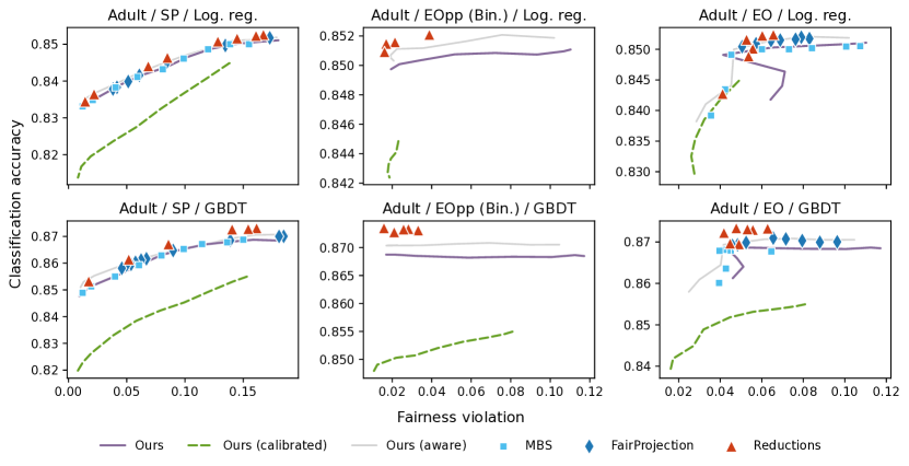
Figure 1: Trade-offs between accuracy and fairness on the Adult dataset. Average of five random seeds. Unless otherwise indicated, the base model is not calibrated and the setting is attribute-blind. The algorithms are configured to satisfy SP, EOpp (binary equal opportunity), or EO, respectively. Fairness violation is measured uniformly (cf. definitions in Table 1). The calibration error of uncalibrated base model under the attribute-blind setting is 0.5785 for logistic regression, and 0.5665 for GBDT.

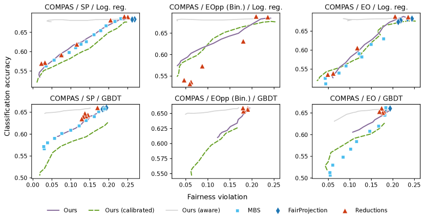
Figure 2: Trade-offs between accuracy and fairness on the COMPAS dataset. EOpp is binary equal opportunity. The calibration error is 0.1589 for logistic regression, and 0.5551 for GBDT.

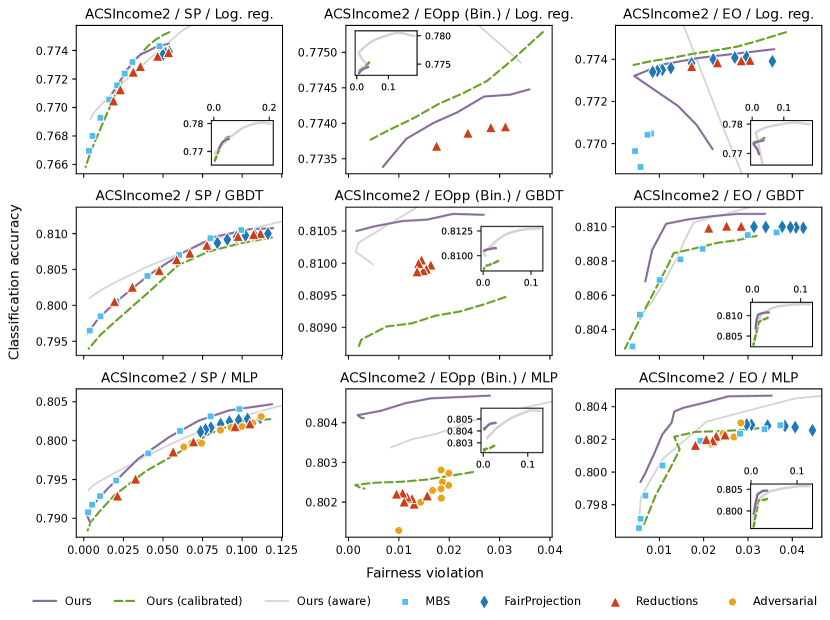
Figure 3: Trade-offs between accuracy and fairness on the ACSIncome2 dataset. EOpp is binary equal opportunity. The calibration error is 0.1700 for logistic regression, 0.1471 for GBDT, and 0.1405 for MLP.

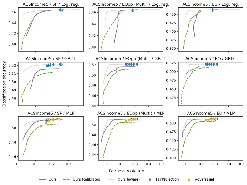
Figure 4: Trade-offs between accuracy and fairness on the ACSIncome5 dataset. EOpp is multi-class equal opportunity. The calibration error is 0.7839 for logistic regression, 1.5936 for GBDT, and 0.7523 for MLP.

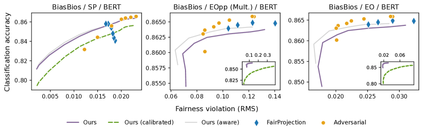
Figure 5: Trade-offs between accuracy and fairness on the BiasBios dataset from varying fairness tolerance. EOpp is multi-class equal opportunity. Fairness violation is measured by taking the root mean square of the disparities (across $y\in\mathcal{Y}$ for SP and EOpp, and $y,y^{\prime}\in\mathcal{Y}$ for EO); the RMS violation of EOpp is the same as the $\mathit{GAP}^{\textrm{TPR},\textrm{RMS}}$ measure in (Ravfogel et al., 2020). The calibration error is 1.7358.

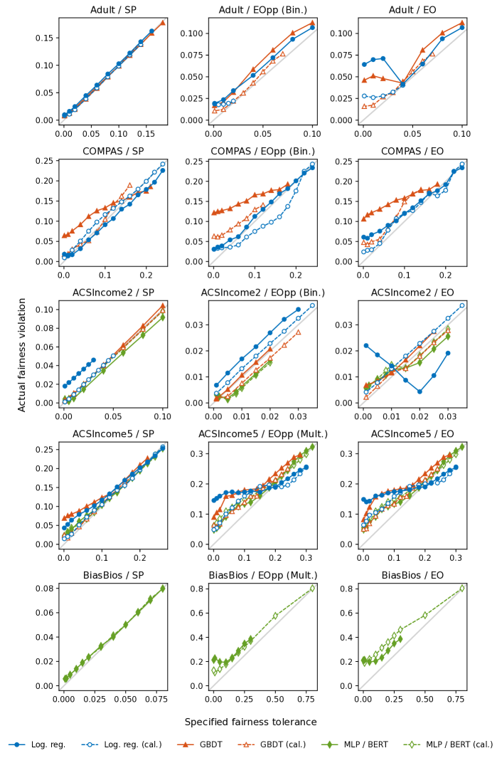
Figure 7: Specified fairness tolerance $\alpha$ plotted against the actual achieved level of fairness by our algorithm, under the attribute-blind setting in Section 4. Average of five random seeds.

Figures 1, 2, 3, 4 and 5 plot the accuracy-fairness trade-offs achieved by the fair algorithms configured to satisfy SP, EOpp, or EO, respectively, from varying the fairness tolerance $\alpha$, and with various base models. All results are averaged over five random seeds, used for splitting the post-processing/test sets, model initialization, and the smoothing noise (standard deviations can be found in our repository1). The settings of $\alpha$ for our algorithm are plotted in Fig. 7 against the achieved levels of fairness, which mostly agree until when $\alpha$ is small and/or $\hat{\tilde{\gamma}}$ possibly deviates significantly from $\gamma$ (more discussions below). The post-processing running times are reported in Table 2 to demonstrate its efficiency (note that EO on BiasBios requires $\sum_{c}|\mathcal{Z}_{c}|=2\cdot 28^{2}$ constraints).

Comparison with Baselines.

First, we remark that because the base models required or learned by the algorithms are different, so may be the upper-right starting points of the respective algorithms (corresponding to results under the most relaxed fairness settings). Our algorithm share the same model with MBS that predicts $\operatorname{\mathbb{P}}(A,Y\mid X)$. The base models required by FairProjection are $\operatorname{\mathbb{P}}(Y\mid X)$, $\operatorname{\mathbb{P}}(A\mid X)$, and $\operatorname{\mathbb{P}}(A\mid X,Y)$. Adversarial yields a single $\operatorname{\mathbb{P}}(Y\mid X)$ predictors, whereas Reductions returns a randomized combination of them (hence this is the most compute-intensive).

Our algorithm is more favorable in the high fairness regime (from setting small $\alpha$). In the low fairness regime (large $\alpha$ settings), on multi-class multi-group problems (ACSIncome5 and BiasBios), our algorithm has lower accuracies than FairProjection and Adversarial likely because the predictor $\operatorname{\mathbb{P}}(A,Y\mid X)$ required by our algorithm is harder to train than $\operatorname{\mathbb{P}}(Y\mid X)$. This could be improved by simplifying the modeling problem with re-parameterization, and/or leveraging label hierarchy.

Compared to in-processing algorithms, although they can theoretically achieve better performance (especially vs. post-processing algorithm with inaccurate base models), optimization is a major difficulty with them. The convergence of the Reductions algorithm to the optimal fair classifier requires repeatedly training and combining a large number of classifiers, so while it has good performance on the smaller UCI Adult dataset (Fig. 1), it underperforms on the larger ACSIncome2 (Fig. 3) under limited compute budget (i.e., number of iterations). The performance of Adversarial training is affected by its instability, partly due to the difficulty in maintaining the optimality of the adversary, and having a conflicting optimization objective (loss minimization vs. fairness).

Comparing to MBS, since it shares a similar underlying framework with ours, we expect similar performance when $M$ is sufficiently large (relative to the data size). It underperforms on the larger problem of post-processing for EO on ACSIncome2. MBS can sometimes achieve higher fairness because it learns parameters on a labeled validation set with $A,Y$ annotations, whereas our algorithm does not use labeled data but the base model’s predicted group membership and label. This performance gap appears only when the base model has a large error (i.e., $(\tilde{\ell},\hat{\tilde{\gamma}})\neq(\ell,\gamma)$) due to small data size (Adult and COMPAS) and/or model misspecification.

Calibration.

We additionally plot the post-processing results of our algorithm with calibrated $\operatorname{\mathbb{P}}(A,Y\mid X)$ predictors. It is observed that calibration allows our algorithm to achieve fairness more precisely to the setting of $\alpha$ (Fig. 7), as well as higher levels of fairness, corroborating the results in Corollaries 3.12 and 3.13. The estimated calibration error (Eq. 34) of the uncalibrated predictor mostly correlates with the improvement in fairness on each dataset.

The calibration method is based on binning, where the output space $\Delta^{\mathcal{A}\times\mathcal{Y}}$ of the base model is partitioned into $k$ bins, each assigned a calibrated value (computed on a holdout set) to which outputs falling into the corresponding bin are remapped. The bins are Voronoi cells with centroids selected using the $k$-means algorithm. The base model is retrained on this set of experiments because the pre-training set needs to be further split for calibration. On the Adult and COMPAS datasets, the split ratio is 0.2/0.8 for training and calibration, and $k=10$; on the remaining datasets, the split ratio is 0.7/0.3 and $k=70$. Note that both binning and dataset splitting hurt model accuracy, due to limited representation power and less samples for training, respectively.

Attribute-Blind vs. Aware.

We compare our algorithm under the attribute-aware and blind settings. Because the attribute-aware predictor can use the extra feature $A$, it always achieve higher accuracy. And, its trade-off curves generally dominate those under the blind setting, but not always in the high fairness regime, which we suspect is likely due to having a larger deviation of $\hat{\tilde{\gamma}}$ from the Bayes optimal $\gamma$.

Performance Under Small $\alpha$.

The lines in the plots connect the results from our algorithm with adjacent fairness tolerance $\alpha$ settings, with smaller $\alpha$ corresponding to higher fairness. When $\alpha$ is small, higher fairness is achieved on the empirical problem $(\tilde{\ell},\hat{\tilde{\gamma}},\widehat{\mathbb{P}}_{X})$, but this improvement may not transfer to the population level (also see Fig. 7); moreover, accuracy may degrade significantly. In practice, we suggest tuning $\alpha$ on a validation set.

There are two reasons for this phenomenon. The first is sample variance: higher fairness on the empirical problem under small $\alpha$ requires fitting the parameters $\tilde{\psi}$ more precisely to the training set, which may overfit and causing high variance. The second is the deviation of $\hat{\tilde{\gamma}}$ from the Bayes optimal $\gamma$: exact fairness cannot be guaranteed without accurate group membership information as reflected in the bounds in Theorem 3.11; accuracy could be improved with stronger approximators (e.g., neural models) and better estimations. The observation that the loss is more sensitive to the deviation as $\alpha\rightarrow 0$ corroborates the bound.

5 Conclusion and Limitations

By reformulating and analyzing the fair classification problem as a linear program, we showed that optimal fair classifiers can be represented by linear post-processings of the loss function and group membership predictors. Following the result, we proposed a post-processing-based fair classification algorithm for parity group fairness constraints and both attribute-aware and blind settings.

Threshold-Invariance.

In some use cases, the practitioner may need to change the threshold of the classifier after deployment, e.g., for adjusting the acceptance rate, or responding to a label shift of the underlying distribution (Lipton et al., 2018). However, under our framework, fairness is not preserved under changes to the threshold of the scores computed by our post-processed classifier (Eq. 19). Instead, post-processing needs to be re-performed for the above scenarios on a re-weighted (fair) classification problem by the ratio of the new marginal class distribution to the old one.

Threshold-invariant fairness is an open problem (Chen and Wu, 2020), with the ultimate goal of computing fair scores that are capable of exploring the Pareto front of the recalls of each class simply by varying the threshold (i.e., in binary classification, the upper boundary of the feasible combinations of TPR and FPR subject to fairness).

Interpretability.

The optimal (binary) classifier subject to statistical parity (under the attribute-aware setting) has a clear interpretation: accept if the individual is in the top-$p$% of the respective group (ranked by the scores), with the same $p$ for all groups. But the effects of imposing more general fairness criteria to the classifier are not as clear (even from Eq. 19), and consequently, decisions made by the classifier may be hard to justify on the individual level, despite being fair on the group level. In particular, Chen et al. (2024) observed that whether an individual is accepted or not can change (unpredictably) as the EO fairness tolerance varies.

This is not a limitation of our framework but of parity group fairness algorithms in general. Improving interpretability would necessitate better understanding and designs of fairness criteria.

Appendix A Omitted Proofs and Discussions

We provide the deferred proofs and discussions here. The proof of Theorem 3.10 is in Appendix B.

Derivation of Dual LP.

The Lagrangian of Primal LP is

$$L(\pi,q,\phi,\psi^{+},\psi^{-}) =\int_{\mathcal{X}}\sum_{y\in\mathcal{Y}}\ell(x,y)\pi(x,y)\mathop{}\!\mathrm{d}\mathbb{P}_{X}(x)$$ (39)

$$\qquad+\int_{\mathcal{X}}\left\lparen 1-\sum_{y\in\mathcal{Y}}\pi(x,y)\right\rparen\phi(x)\mathop{}\!\mathrm{d}\mathbb{P}_{X}(x)$$ (40)

$$\qquad+\sum_{c}\sum_{z\in\mathcal{Z}_{c}}\left\lparen-\frac{\alpha}{2}+q_{c}-\int_{\mathcal{X}}\gamma(x,z)\pi(x,y_{c})\mathop{}\!\mathrm{d}\mathbb{P}_{X}(x)\right\rparen\psi^{+}_{c,z}$$ (41)

$$\qquad+\sum_{c}\sum_{z\in\mathcal{Z}_{c}}\left\lparen-\frac{\alpha}{2}+q_{c}+\int_{\mathcal{X}}\gamma(x,z)\pi(x,y_{c})\mathop{}\!\mathrm{d}\mathbb{P}_{X}(x)\right\rparen\psi^{-}_{c,z}$$ (42)

(note that $\sum_{y}\pi(x,y)=1\iff\sum_{y}\pi(x,y)\operatorname{\mathbb{P}}_{X}(x)=\operatorname{\mathbb{P}}_{X}(x)$, $\forall x\in\operatorname{supp}(\mathbb{P}_{X})$). Collecting terms, we get

$$L(\pi,q,\phi,\psi^{+},\psi^{-})$$ (43)

$$=\begin{multlined}\int_{\mathcal{X}}\phi(x)\mathop{}\!\mathrm{d}\mathbb{P}_{X}(x)+\sum_{c}\sum_{z\in\mathcal{Z}_{c}}\left\lparen q_{c}(\psi^{+}_{c,z}-\psi^{-}_{c,z})-\frac{\alpha}{2}(\psi^{+}_{c,z}+\psi^{-}_{c,z})\right\rparen\\ +\int_{\mathcal{X}}\sum_{y\in\mathcal{Y}}\Bigg{(}\ell(x,y)-\underbrace{\phi(x)+\sum_{c}\operatorname{\mathds{1}}[y_{c}=y]\sum_{z\in\mathcal{Z}_{c}}(\psi^{+}_{c,z}-\psi^{-}_{c,z})\gamma(x,z)}_{(\star)}\Bigg{)}\pi(x,y)\mathop{}\!\mathrm{d}\mathbb{P}_{X}(x).\end{multlined}\int_{\mathcal{X}}\phi(x)\mathop{}\!\mathrm{d}\mathbb{P}_{X}(x)+\sum_{c}\sum_{z\in\mathcal{Z}_{c}}\left\lparen q_{c}(\psi^{+}_{c,z}-\psi^{-}_{c,z})-\frac{\alpha}{2}(\psi^{+}_{c,z}+\psi^{-}_{c,z})\right\rparen\\ +\int_{\mathcal{X}}\sum_{y\in\mathcal{Y}}\Bigg{(}\ell(x,y)-\underbrace{\phi(x)+\sum_{c}\operatorname{\mathds{1}}[y_{c}=y]\sum_{z\in\mathcal{Z}_{c}}(\psi^{+}_{c,z}-\psi^{-}_{c,z})\gamma(x,z)}_{(\star)}\Bigg{)}\pi(x,y)\mathop{}\!\mathrm{d}\mathbb{P}_{X}(x).$$ (46)

By strong duality, $\min_{\pi\geq 0}\max_{\phi,\psi^{+}\geq 0,\psi^{-}\geq 0}L=\max_{\phi,\psi^{+}\geq 0,\psi^{-}\geq 0}\min_{\pi\geq 0}L$. If $\ell(x,y)<(\star)$ for some $(x,y)$, then we can send $L$ to $-\infty$ by setting $\pi(x,y)=\infty$, so we must have that $\ell(x,y)\geq(\star)$ for all $x,y$. But with this constraint, the best we can do for $\min_{\pi\geq 0}L$ is to set $\pi=0$, so the last line is omitted. Similarly, we must have $\sum_{z\in\mathcal{Z}_{c}}(\psi^{+}_{c,z}-\psi^{-}_{c,z})=0$ by considering its interaction with $q_{c}$. ∎

Proof of Theorem 3.3.

Let $(\pi,q)$ be a minimizer of Primal LP and $(\phi,\psi)$ the associated dual variables (maximizer of Dual LP). By the definition of LP, the randomized classifier that outputs $y$ with probability $\propto\pi(x,y)$, given each $x$, is an optimal classifier satisfying $\alpha$-parity w.r.t. $\mathcal{C}$.

Complementary slackness states that $\pi(x,y)>0\iff\phi(x)-g_{\ell,\gamma,\psi}(x,y)=0$ (Papadimitriou and Steiglitz, 1998), and we show that it implies

$$\pi(x,y)>0\implies y\in\operatorname*{arg\,min}_{y^{\prime}\in\mathcal{Y}}g_{\ell,\gamma,\psi}(x,y^{\prime}).$$ (47)

Suppose not, then $\exists z\neq y$ such that $g_{\ell,\gamma,\psi}(x,z)-g_{\ell,\gamma,\psi}(x,y)<0$. By the first constraint in Dual LP, we know that $\phi(x)-g_{\ell,\gamma,\psi}(x,z)\leq 0$. Adding the two inequalities together, we get $\phi(x)-g_{\ell,\gamma,\psi}(x,y)<0$, which contradicts the result from complementary slackness.

By Assumption 3.2, we have that $|\operatorname*{arg\,min}_{y}g_{\ell,\gamma,\psi}(x,y)|=1$ almost surely. This together with Eq. 47 imply that

$$x\mapsto\operatorname*{arg\,min}_{y\in\mathcal{Y}}g_{\ell,\gamma,\psi}(x,y)=h_{\ell,\gamma,\psi}(x)$$ (48)

is an optimal classifier satisfying $\alpha$-parity w.r.t. $\mathcal{C}$, since it agrees with the randomized classifier derived from $\pi$ described above almost everywhere. ∎

Proof of Lemma 3.7.

Let any linear subspace described in Assumption 3.6 be given by $\{(u,v):a^{\top}u+b^{\top}v=0\}$ for some $a\in\mathbb{R}^{\mathcal{Z}}$, $b\in\mathbb{R}^{\mathcal{Y}}$ and $b\neq 0$. Then

$$\operatorname{\mathbb{P}}_{U,V}(\{(u,v):a^{\top}u+b^{\top}v=0\})$$ (49)

$$=\operatorname{\mathbb{P}}_{U,V}(a^{\top}U+b^{\top}V=0)$$ (50)

$$=\operatorname{\mathbb{P}}_{X,\varepsilon}\left\lparen\sum_{y\in\mathcal{Y}}b_{y}\varepsilon_{y}=-\sum_{y\in\mathcal{Y}}b_{y}\ell(X,y)-\sum_{z\in\mathcal{Z}}a_{z}\gamma(X,z)\right\rparen$$ (51)

$$=\operatorname{\mathbb{E}}_{X}\operatorname{\mathbb{P}}_{\varepsilon\mid X}\left\lparen\sum_{y\in\mathcal{Y}}b_{y}\varepsilon_{y}=-\sum_{y\in\mathcal{Y}}b_{y}\ell(X,y)-\sum_{z\in\mathcal{Z}}a_{z}\gamma(X,z)\right\rparen$$ (52)

$$=0,$$ (53)

because $\sum_{y}b_{y}\varepsilon_{y}$ is a non-zero combination of independent random variables with a continuous distribution, and is independent of $X$. ∎

Before the proving Theorem 3.11, note the fact that a classifier $h$ whose output does not depend on the input satisfies $0$-parity (e.g., the constant predictor), that is, for some probability vector $p\in\Delta^{\mathcal{Y}}$, the output distribution $\operatorname{\mathbb{P}}(h(X)=y\mid X=x)=p_{y}$ is the same for all inputs $x$:

Proposition A.1.

Let $p\in\Delta^{\mathcal{Y}}$, and $\pi(x,\cdot)=p$, $\forall x\in\mathcal{X}$. Then for any constraint function $\gamma$ (Eq. 6) and parity fairness criterion $\mathcal{C}=\{(\mathcal{Z}_{c},y_{c})\}_{c}$ (Definition 2.2),

$$\max_{z,z^{\prime}\in\mathcal{Z}_{c}}\left|\operatorname{\mathbb{E}}_{X}\lparen\gamma(X,z)-\gamma(X,z^{\prime})\rparen\pi(X,y_{c})\right|=0,\quad\forall c.$$ (54)

Proof.

It simply follows from the fact that, $\forall c$ and $z\in\mathcal{Z}_{c}$,

$${\int_{\mathcal{X}}\gamma(x,z)\pi(x,y_{c})\mathop{}\!\mathrm{d}\mathbb{P}_{X}(x)} ={\int_{\mathcal{X}}\frac{\operatorname{\mathbb{P}}(Z=z\mid X=x)}{\operatorname{\mathbb{P}}(Z=z)}\pi(x,y_{c})\mathop{}\!\mathrm{d}\mathbb{P}_{X}(x)}$$ (55)

$$=p_{y_{c}}{\int_{\mathcal{X}}\operatorname{\mathbb{P}}(X=x\mid Z=z)\mathop{}\!\mathrm{d}x}$$ (56)

$$=p_{y_{c}}.\qed$$ (57)

Proof of Theorem 3.11.

For clarity, we denote

$$\langle\ell,\pi\rangle \coloneqq\sum_{y\in\mathcal{Y}}\operatorname{\mathbb{E}}_{X}\ell(X,y)\pi(X,y),$$ (58)

$$\langle\gamma_{z},\pi_{y}\rangle \coloneqq\operatorname{\mathbb{E}}_{X}\gamma(X,z)\pi(X,y)\quad\text{where}\quad\gamma_{z}(x)\coloneqq\gamma(x,z),\,\pi_{y}(x)\coloneqq\pi(x,y).$$ (59)

Part 1 (Deviation of $\ell^{\prime}\neq\ell$).

Because both $\pi,\pi^{\prime}$ are feasible solutions to $\hyperlink{eq:primal}{\textnormal{Primal LP}}(\ell,\gamma,\mathbb{P}_{X},\alpha)$ and $\hyperlink{eq:primal}{\textnormal{LP}}(\ell^{\prime},\gamma,\mathbb{P}_{X},\alpha)$, and are minimizers of the respective problems, we have

$$0 \leq\langle\ell,\pi^{\prime}\rangle-\langle\ell,\pi\rangle$$ (60)

$$=\langle\ell-\ell^{\prime},\pi^{\prime}\rangle+\langle\ell^{\prime},\pi^{\prime}-\pi\rangle+\langle\ell^{\prime}-\ell,\pi\rangle$$ (61)

$$\leq\langle\ell-\ell^{\prime},\pi^{\prime}\rangle+\langle\ell^{\prime}-\ell,\pi\rangle$$ (62)

$$=\langle\ell-\ell^{\prime},\pi^{\prime}-\pi\rangle$$ (63)

$$\leq\sum_{y\in\mathcal{Y}}\operatorname{\mathbb{E}}_{X}|\ell(X,y)-\ell^{\prime}(X,y)|$$ (64)

$$=\varepsilon_{\ell^{\prime}}$$ (65)

by Hölder’s inequality, since $\max_{y}|\pi^{\prime}(x,y)-\pi(x,y)|\leq 1$.

Part 2 (Deviation of $\gamma^{\prime}\neq\gamma$).

We begin with the second result, regarding constraint violation. For all $c$,

$$\max_{z,z^{\prime}\in\mathcal{Z}_{c}}|\langle\gamma_{z}-\gamma_{z^{\prime}},\pi^{\prime}_{y_{c}}\rangle|$$ (66)

$$=\max_{z,z^{\prime}\in\mathcal{Z}_{c}}|\langle\gamma^{\prime}_{z}-\gamma^{\prime}_{z^{\prime}},\pi^{\prime}_{y_{c}}\rangle+\langle\gamma_{z}-\gamma^{\prime}_{z}+\gamma^{\prime}_{z^{\prime}}-\gamma_{z^{\prime}},\pi^{\prime}_{y_{c}}\rangle|$$ (67)

$$\leq\max_{z,z^{\prime}\in\mathcal{Z}_{c}}|\langle\gamma^{\prime}_{z}-\gamma^{\prime}_{z^{\prime}},\pi^{\prime}_{y_{c}}\rangle|+2\max_{z\in\mathcal{Z}_{c}}|\langle\gamma_{z}-\gamma^{\prime}_{z},\pi^{\prime}_{y_{c}}\rangle|$$ (68)

$$\leq\alpha+2\max_{z\in\mathcal{Z}_{c}}|\langle\gamma_{z}-\gamma^{\prime}_{z},\pi^{\prime}_{y_{c}}\rangle|$$ (second constraint of Primal LP) (69)

$$\leq\alpha+2\max_{z\in\mathcal{Z}_{c}}\max_{\pi^{\prime\prime}}|\langle\gamma_{z}-\gamma^{\prime}_{z},\pi^{\prime\prime}_{y_{c}}\rangle|$$ (70)

$$=\alpha+2\max_{z\in\mathcal{Z}_{c}}|\langle(\gamma_{z}-\gamma^{\prime}_{z})_{+},\mathbf{1}\rangle| \pi^{\prime}_{y_{c}}(x)\in[0,1] x$$ ( for all ) (71)

$$=\alpha+\max_{z\in\mathcal{Z}_{c}}\langle|\gamma_{z}-\gamma^{\prime}_{z}|,\mathbf{1}\rangle$$ (72)

$$\leq\alpha+\varepsilon_{\gamma^{\prime}},$$ (73)

where we denoted $(a)_{+}=\max(0,a)$ element-wise. The second last equality uses the fact that $\langle a,\mathbf{1}\rangle=0\implies|\langle a,\mathbf{1}\rangle|=2\langle(a)_{+},\mathbf{1}\rangle$, and we verify that $\langle\gamma_{z}-\gamma^{\prime}_{z},\mathbf{1}\rangle=0$, because by the definition in Eq. 6, $\langle\gamma_{z},\mathbf{1}\rangle=\int_{\mathcal{X}}\gamma(x,z)\mathop{}\!\mathrm{d}\mathbb{P}_{X}(x)=\int\operatorname{\mathbb{P}}(Z=z,X=x)\mathop{}\!\mathrm{d}x/\operatorname{\mathbb{P}}(Z=z)=1$. In addition, similarly,

$$\max_{z,z^{\prime}\in\mathcal{Z}_{c}}|\langle\gamma_{z}-\gamma_{z^{\prime}},\pi^{\prime}_{y_{c}}\rangle| \leq\max_{z,z^{\prime}\in\mathcal{Z}_{c}}\max_{\pi^{\prime}}|\langle\gamma_{z}-\gamma_{z^{\prime}},\pi^{\prime}_{y_{c}}\rangle|$$ (74)

$$=\frac{1}{2}\max_{z,z^{\prime}\in\mathcal{Z}_{c}}|\langle\gamma_{z}-\gamma_{z^{\prime}},\mathbf{1}\rangle|$$ (75)

$$\leq\max_{z\in\mathcal{Z}_{c}}|\langle\gamma_{z},\mathbf{1}\rangle|$$ (76)

$$=1,$$ (77)

so

$$\max_{z,z^{\prime}\in\mathcal{Z}_{c}}|\langle\gamma_{z}-\gamma_{z^{\prime}},\pi^{\prime}_{y_{c}}\rangle|\leq\max(1,\alpha+\varepsilon_{\gamma^{\prime}}),\quad\forall c.$$ (78)

For the first result on the loss, we first construct a feasible solution $\pi^{\prime\prime}$ to $\hyperlink{eq:primal}{\textnormal{Primal LP}}(\ell,\gamma^{\prime},\mathbb{P}_{X},\alpha)$ from $\pi$, whose value upper bounds that of the minimizer $\pi^{\prime}$ of $\hyperlink{eq:primal}{\textnormal{LP}}(\ell,\gamma^{\prime},\mathbb{P}_{X},\alpha)$, then we bound the difference between $\pi$ and $\pi^{\prime\prime}$:

$$\langle\ell,\pi^{\prime}-\pi\rangle\leq\langle\ell,\pi^{\prime\prime}-\pi\rangle\leq\|\ell\|_{\infty}\sum_{y\in\mathcal{Y}}\operatorname{\mathbb{E}}_{X}|\pi^{\prime\prime}(X,y)-\pi(X,y)|.$$ (79)

We set

$$\pi^{\prime\prime}(x,\cdot)=(1-\beta)\pi(x,\cdot)+\beta\mathbf{e}_{1},\quad\forall x\in\mathcal{X}$$ (80)

for $\beta\in[0,1]$, which is a randomized combination of $\pi$ and the constant classifier that always outputs class $1$, then

$$\sum_{y\in\mathcal{Y}}\operatorname{\mathbb{E}}_{X}|\pi^{\prime\prime}(X,y)-\pi(X,y)|\leq\beta\sum_{y\in\mathcal{Y}}\left\lparen\operatorname{\mathbb{E}}_{X}\pi(X,y)+1\right\rparen\leq 2\beta.$$ (81)

Because the constant classifier satisfies $0$-parity (Proposition A.1), and by Eq. 78, the constraint violation of $\pi^{\prime\prime}$ is

$$\max_{z,z^{\prime}\in\mathcal{Z}_{c}}|\langle\gamma_{z}-\gamma_{z^{\prime}},\pi^{\prime\prime}_{y_{c}}\rangle|=(1-\beta)\max_{z,z^{\prime}\in\mathcal{Z}_{c}}|\langle\gamma_{z}-\gamma_{z^{\prime}},\pi^{\prime}_{y_{c}}\rangle|\leq(1-\beta)\min(1,\alpha+\varepsilon_{\gamma^{\prime}}).$$ (82)

For the right hand side to be $\leq\alpha$, we need to set

$$\beta\geq\min\left\lparen 1-\alpha,\frac{\varepsilon_{\gamma^{\prime}}}{\alpha+\varepsilon_{\gamma^{\prime}}}\right\rparen.$$ (83)

Combining with Eqs. 79 and 81, we get

$$\langle\ell,\pi^{\prime}-\pi\rangle \leq 2\|\ell\|_{\infty}\min\left\lparen 1-\alpha,\frac{\varepsilon_{\gamma^{\prime}}}{\alpha+\varepsilon_{\gamma^{\prime}}}\right\rparen.\qed$$ (84)

Proof of Corollary 3.12.

Following the same analysis in the proof of the second result of Part 2 of Theorem 3.11, for all $c$,

$$\max_{z,z^{\prime}\in\mathcal{Z}_{c}}\left|\operatorname{\mathbb{E}}_{X}\lparen\gamma(X,z)-\gamma(X,z^{\prime})\rparen\operatorname{\mathds{1}}[h_{\ell,\gamma^{\prime},\psi}(X)=y_{c}]\right|$$ (85)

$$\leq\alpha+\varepsilon^{\textnormal{cal}}_{\gamma^{\prime}}+2\max_{z\in\mathcal{Z}_{c}}\left|\operatorname{\mathbb{E}}_{X}\lparen\gamma(X,z)-\gamma^{\textnormal{cal}}(X,z)\rparen\operatorname{\mathds{1}}[h_{\ell,\gamma^{\prime},\psi}(X)=y_{c}]\right|.$$ (86)

Define

$$\operatorname{\mathbb{P}}^{\textnormal{cal}}(Z=z\mid X=x)=f_{z}^{\textnormal{cal}}(x),$$ (87)

and by calibration,

$$\operatorname{\mathbb{P}}^{\textnormal{cal}}(Z=z)\coloneqq{} \operatorname{\mathbb{E}}_{X}f_{z}^{\textnormal{cal}}(X)$$ (88)

$$={} \int_{\mathcal{X}}\operatorname{\mathbb{P}}^{\textnormal{cal}}(Z=z\mid X=x)\mathop{}\!\mathrm{d}\mathbb{P}_{X}(x)$$ (89)

$$={} \int_{\mathcal{X}}\operatorname{\mathbb{P}}(Z=z\mid f(X)=f(x),\ell(X,\cdot)=\ell(x,\cdot))\mathop{}\!\mathrm{d}\mathbb{P}_{X}(x)$$ (90)

$$={} \int_{\mathbb{R}^{\mathcal{Z}}\times\mathbb{R}^{\mathcal{Y}}}\operatorname{\mathbb{P}}(Z=z\mid U^{\prime}=u,V=v)\mathop{}\!\mathrm{d}\mathbb{P}_{U^{\prime},V}(u,v)$$ (91)

$$={} \operatorname{\mathbb{P}}(Z=z)$$ (92)

where $(u,v)$ takes values in the feature space $\mathbb{R}^{\mathcal{Z}}\times\mathbb{R}^{\mathcal{Y}}$ of $(U^{\prime},V)=(f(X),\ell(X,\cdot))$; line 3 is by definition of $f^{\textnormal{cal}}$, and line 4 is because the integrand on the preceding line is piece-wise constant. Then

$$\operatorname{\mathbb{E}}_{X}\lparen\gamma(X,z)-\gamma^{\textnormal{cal}}(X,z)\rparen\operatorname{\mathds{1}}[h_{\ell,\gamma^{\prime},\psi}(X)=y_{c}]$$ (93)

$$=\int_{\mathcal{X}}\left\lparen\frac{\operatorname{\mathbb{P}}(Z=z\mid X=x)}{\operatorname{\mathbb{P}}(Z=z)}-\frac{\operatorname{\mathbb{P}}^{\textnormal{cal}}(Z=z\mid X=x)}{\operatorname{\mathbb{P}}^{\textnormal{cal}}(Z=z)}\right\rparen\operatorname{\mathds{1}}[h_{\ell,\gamma^{\prime},\psi}(x)=y_{c}]\mathop{}\!\mathrm{d}\mathbb{P}_{X}(x)$$ (94)

$$=\frac{1}{\operatorname{\mathbb{P}}(Z=z)}\int_{\mathcal{X}}\left\lparen\operatorname{\mathbb{P}}(Z=z\mid X=x)-\operatorname{\mathbb{P}}^{\textnormal{cal}}(Z=z\mid X=x)\right\rparen\operatorname{\mathds{1}}[h_{\ell,\gamma^{\prime},\psi}(x)=y_{c}]\mathop{}\!\mathrm{d}\mathbb{P}_{X}(x)$$ (95)

$$=\begin{multlined}\frac{1}{\operatorname{\mathbb{P}}(Z=z)}\sum_{u,v}\int_{\mathcal{X}}\left\lparen\operatorname{\mathbb{P}}(Z=z\mid X=x)-\operatorname{\mathbb{P}}^{\textnormal{cal}}(Z=z\mid X=x)\right\rparen\\ \operatorname{\mathds{1}}[f(x)=u,\ell(x,\cdot)=v]\operatorname{\mathds{1}}[h_{\ell,\gamma^{\prime},\psi}(x)=y_{c}]\mathop{}\!\mathrm{d}\mathbb{P}_{X}(x).\end{multlined}\frac{1}{\operatorname{\mathbb{P}}(Z=z)}\sum_{u,v}\int_{\mathcal{X}}\left\lparen\operatorname{\mathbb{P}}(Z=z\mid X=x)-\operatorname{\mathbb{P}}^{\textnormal{cal}}(Z=z\mid X=x)\right\rparen\\ \operatorname{\mathds{1}}[f(x)=u,\ell(x,\cdot)=v]\operatorname{\mathds{1}}[h_{\ell,\gamma^{\prime},\psi}(x)=y_{c}]\mathop{}\!\mathrm{d}\mathbb{P}_{X}(x).$$ (98)

Since $h_{\ell,\gamma^{\prime},\psi}$ is a linear classifier on the features $(U^{\prime},V)$ following the discussion in Eq. 19, it assigns the same class to all $x$ that share the same output value of $(f(x),\ell(x,\cdot))$. This means that when $(u,v)$ is fixed, for all $x$ such that $f(x)=u$ and $\ell(x,\cdot)=v$, $\operatorname{\mathds{1}}[h_{\ell,\gamma^{\prime},\psi}(x)=y_{c}]$ is either always $0$ or always $1$. In the first case, Eq. 93 is zero. In the second case,

$$\int_{\mathcal{X}}\operatorname{\mathbb{P}}^{\textnormal{cal}}(Z=z\mid X=x)\operatorname{\mathds{1}}[f(x)=u,\ell(x,\cdot)=v]\mathop{}\!\mathrm{d}\mathbb{P}_{X}(x)$$ (99)

$$=\operatorname{\mathbb{P}}^{\textnormal{cal}}(Z=z\mid X=x^{\prime})\operatorname{\mathbb{P}}_{U^{\prime},V}(u,v)$$ (100)

$$=f_{z}^{\textnormal{cal}}(x^{\prime})\operatorname{\mathbb{P}}_{U^{\prime},V}(u,v)$$ (101)

for all $x^{\prime}$ satisfying $f(x^{\prime})=u$ and $\ell(x^{\prime},\cdot)=v$ because $\operatorname{\mathbb{P}}^{\textnormal{cal}}(Z=z\mid X=x^{\prime})$ is constant on all such $x^{\prime}$ by Eq. 33; and on the other hand,

$$\int_{\mathcal{X}}\operatorname{\mathbb{P}}(Z=z\mid X=x)\operatorname{\mathds{1}}[f(x)=u,\ell(x,\cdot)=v]\mathop{}\!\mathrm{d}\mathbb{P}_{X}(x)$$ (102)

$$=\operatorname{\mathbb{P}}(Z=z\mid f(X)=u,\ell(X,\cdot)=v)\operatorname{\mathbb{P}}(f(X)=u,\ell(X,\cdot)=v)$$ (103)

$$=\operatorname{\mathbb{P}}(Z=z\mid f(X)=u,\ell(X,\cdot)=v)\operatorname{\mathbb{P}}_{U^{\prime},V}(u,v)$$ (104)

$$=\operatorname{\mathbb{P}}(Z=z\mid f(X)=f(x^{\prime}),\ell(X,\cdot)=\ell(x^{\prime},\cdot))\operatorname{\mathbb{P}}_{U^{\prime},V}(u,v)$$ (105)

$$=f_{z}^{\textnormal{cal}}(x^{\prime})\operatorname{\mathbb{P}}_{U^{\prime},V}(u,v)$$ (106)

by Eq. 33. So the difference between Eqs. 99 and 102 is zero, hence Eq. 93 is always zero. ∎

Figure 6: The upper bound in Theorem 3.11 for the sub-optimality due to the constraint function deviating from the Bayes optimal by $\varepsilon$, plotted for different tolerances $\alpha\in[0,1]$. Example A.2 matches the shaded region up to a constant factor.

Example A.2.

We construct problem instances matching the upper bound for sub-optimality in Theorem 3.11 Part 2 up to a constant factor (see Fig. 6). The problem is constructed such that the optimal unconstrained classifier is already fair w.r.t. the true constraint $\gamma$, but not w.r.t. the non-optimal constraint $\gamma^{\prime}$, so a loss is incurred from satisfying $\gamma^{\prime}$.

Consider post-processing for statistical parity under the attribute-blind setting for binary classification ($|\mathcal{Y}|=2$) with classification error as the loss. We specify the data distribution as follows:

• $|\mathcal{A}|=2$, and $\operatorname{\mathbb{P}}(A=0)=\operatorname{\mathbb{P}}(A=1)=1/2$.

• $\mathcal{X}=\{0,1\}$, and $\operatorname{\mathbb{P}}(X=0\mid A=0)\in[0,1/2]$ (which we can vary to construct different problem instances), and let $\operatorname{\mathbb{P}}(X=0\mid A=1)=1-\operatorname{\mathbb{P}}(X=0\mid A=0)$.

  Note that $\mathbb{P}_{X}$ is uniform by construction, because $\operatorname{\mathbb{P}}(X=0)=\sum_{a\in\{0,1\}}\operatorname{\mathbb{P}}(X=0\mid A=a)\operatorname{\mathbb{P}}(A=a)=1/2=\operatorname{\mathbb{P}}(X=1)$.

• $\operatorname{\mathbb{P}}(Y=0\mid X=0)=\operatorname{\mathbb{P}}(Y=1\mid X=1)=1$. This appears in the loss function $\ell$.

By construction, the constraint function $\gamma$ is:

$$\gamma(0,0) =\frac{\operatorname{\mathbb{P}}(A=0\mid X=0)}{\operatorname{\mathbb{P}}(A=0)}$$ (107)

$$=\frac{\operatorname{\mathbb{P}}(X=0\mid A=0)}{\operatorname{\mathbb{P}}(X=0)}$$ (108)

$$=2\operatorname{\mathbb{P}}(X=0\mid A=0)$$ (109)

$$=2(1-\operatorname{\mathbb{P}}(X=1\mid A=0))$$ (110)

$$=2-\frac{\operatorname{\mathbb{P}}(A=0\mid X=1)}{\operatorname{\mathbb{P}}(A=0)}$$ (111)

$$=2-\gamma(1,0)$$ (112)

(similarly for $\gamma(\cdot,1)$).

Define $\pi_{x}\coloneqq\pi(x,1)=\operatorname{\mathbb{P}}(h(X)=1\mid X=x)$, $\forall x\in\{0,1\}$, representing the randomized classifier. Statistical parity requires that

$$\alpha \geq\left|\pi_{0}\left\lparen\gamma(0,0)-\gamma(0,1)\right\rparen\operatorname{\mathbb{P}}(X=0)+\pi_{1}\left\lparen\gamma(1,0)-\gamma(1,1)\right\rparen\operatorname{\mathbb{P}}(X=1)\right|$$ (113)

$$=\left|\frac{\pi_{0}}{2}\left\lparen\frac{\operatorname{\mathbb{P}}(A=0\mid X=0)}{\operatorname{\mathbb{P}}(A=0)}-\frac{\operatorname{\mathbb{P}}(A=1\mid X=0)}{\operatorname{\mathbb{P}}(A=1)}\right\rparen+\frac{\pi_{1}}{2}\left\lparen\frac{\operatorname{\mathbb{P}}(A=0\mid X=1)}{\operatorname{\mathbb{P}}(A=0)}-\frac{\operatorname{\mathbb{P}}(A=1\mid X=1)}{\operatorname{\mathbb{P}}(A=1)}\right\rparen\right|$$ (114)

$$=\left|(\operatorname{\mathbb{P}}(X=0\mid A=0)-\operatorname{\mathbb{P}}(X=0\mid A=1))(\pi_{0}-\pi_{1})\right|$$ (115)

$$=\left|(1-2\operatorname{\mathbb{P}}(X=0\mid A=0))(\pi_{0}-\pi_{1})\right|$$ (116)

$$\eqqcolon\delta\left|\pi_{0}-\pi_{1}\right|,$$ (117)

which is if and only if $\left|\pi_{0}-\pi_{1}\right|\leq\alpha/\delta$. Note that $\delta\in[0,1]$ as we can specify $\operatorname{\mathbb{P}}(X=0\mid A=0)\in[0,1/2]$ in the construction. We can rewrite $\hyperlink{eq:primal}{\textnormal{Primal LP}}(\ell,\gamma,\alpha)$ as

$$\min_{\pi_{0},\pi_{1}\in[0,1]}\frac{1}{2}+\frac{1}{2}(\pi_{0}-\pi_{1})\quad\mathrm{s.t.}\quad\left|\pi_{0}-\pi_{1}\right|\leq\frac{\alpha}{\delta},$$ (118)

whose optimal value is $1/2\cdot\max(1-\alpha/\delta,0)$, attained by setting $\pi_{0}=0$ and $\pi_{1}=\min(\alpha/\delta,1)$ (here with $0/0\coloneqq\infty$).

Now, let the non-optimal constraint function $\gamma^{\prime}$ be $\operatorname{\mathbb{P}}^{\prime}(X=0\mid A=0)\in[0,\operatorname{\mathbb{P}}(X=0\mid A=0)]$, and let $\operatorname{\mathbb{P}}^{\prime}(X=0\mid A=0)=1-\operatorname{\mathbb{P}}^{\prime}(X=0\mid A=1)$. Denote the $L^{1}(\mathbb{P}_{X})$ difference in the constraint function by

$$\varepsilon =\frac{1}{2}\left\|\frac{\operatorname{\mathbb{P}}(A=0\mid X=\cdot)}{\operatorname{\mathbb{P}}(A=0)}-\frac{\operatorname{\mathbb{P}}^{\prime}(A=0\mid X=\cdot)}{\operatorname{\mathbb{P}}(A=0)}\right\|_{1}$$ (119)

$$=\left\|\operatorname{\mathbb{P}}(X=\cdot\mid A=0)-\operatorname{\mathbb{P}}^{\prime}(X=\cdot\mid A=0)\right\|_{1}$$ (120)

$$=2\left|\operatorname{\mathbb{P}}(X=0\mid A=0)-\operatorname{\mathbb{P}}^{\prime}(X=0\mid A=0)\right|$$ (121)

$$\in[0,1-\delta].$$ (122)

Then, similarly, $\hyperlink{eq:primal}{\textnormal{Primal LP}}(\ell,\gamma^{\prime},\alpha)$ with the non-optimal constraint function can be rewritten as

$$\min_{\pi^{\prime}_{0},\pi^{\prime}_{1}\in[0,1]}\frac{1}{2}+\frac{1}{2}(\pi^{\prime}_{0}-\pi^{\prime}_{1})\quad\mathrm{s.t.}\quad\left|\pi^{\prime}_{0}-\pi^{\prime}_{1}\right|\leq\frac{\alpha}{\delta^{\prime}}$$ (123)

with optimal value $1/2\cdot\max(1-\alpha/\delta^{\prime},0)$, where

$$\delta^{\prime}=1-2\operatorname{\mathbb{P}}^{\prime}(X=0\mid A=0)=1-2\left\lparen\operatorname{\mathbb{P}}(X=0\mid A=0)-\frac{\varepsilon}{2}\right\rparen=\delta+\varepsilon.$$ (124)

Therefore, given any $\alpha\in[0,1]$, a problem instance can be constructed (i.e., the one above and setting $\delta=\alpha$) such that upon changes in the constraint function by $\varepsilon\in[0,1-\alpha]$ (see Fig. 6), the change in the value is

$$\frac{1}{2}\max\left\lparen 1-\frac{\alpha}{\delta+\varepsilon},0\right\rparen-\frac{1}{2}\max\left\lparen 1-\frac{\alpha}{\delta},0\right\rparen=\frac{1}{2}\left\lparen 1-\frac{\alpha}{\alpha+\varepsilon}\right\rparen=\frac{1}{2}\left\lparen\frac{\varepsilon}{\alpha+\varepsilon}\right\rparen,$$ (125)

which matches the upper bound in Theorem 3.11 by a factor $1/4$.

Appendix B Proof of Theorem 3.10

The proof uses concentration inequality and uniform convergence results, as well as a bound on the complexity of $\mathcal{H}_{\ell,\gamma}$. We recall the definition of VC dimension and pseudo-dimension, and relevant uniform convergence bounds.

Definition B.1 (Shattering).

Let $\mathcal{H}$ be a class of binary functions from $\mathcal{X}$ to $\{0,1\}$. A set $\{x_{1},\dots,x_{n}\}\subseteq\mathcal{X}$ is said to be shattered by $\mathcal{H}$ if $\forall b_{1},\dots,b_{n}\in\{0,1\}$ binary labels, $\exists h\in\mathcal{H}$ s.t. $h(x_{i})=b_{i}$ for all $i\in[n]$.

Definition B.2 (VC Dimension).

Let $\mathcal{H}$ be a class of binary functions from $\mathcal{X}$ to $\{0,1\}$. The VC dimension of $\mathcal{H}$, denoted by $d_{\textnormal{VC}}(\mathcal{H})$, is the size of the largest subset of $\mathcal{X}$ shattered by $\mathcal{H}$.

Definition B.3 (Pseudo-Shattering).

Let $\mathcal{F}$ be a class of functions from $\mathcal{X}$ to $\mathbb{R}$. A set $\{x_{1},\dots,x_{n}\}\subseteq\mathcal{X}$ is said to be pseudo-shattered by $\mathcal{F}$ if $\exists t_{1},\dots,t_{n}\in\mathbb{R}$ threshold values s.t. $\forall b_{1},\dots,b_{n}\in\{0,1\}$ binary labels, $\exists f\in\mathcal{F}$ s.t. $\operatorname{\mathds{1}}[f(x_{i})\geq t_{i}]=b_{i}$ for all $i\in[n]$.

Definition B.4 (Pseudo-Dimension).

Let $\mathcal{F}$ be a class of functions from $\mathcal{X}$ to $\mathbb{R}$. The pseudo-dimension of $\mathcal{F}$, denoted by $d_{\textnormal{P}}(\mathcal{F})$, is the size of the largest subset of $\mathcal{X}$ pseudo-shattered by $\mathcal{F}$.

Theorem B.5 (Pseudo-Dimension Uniform Convergence).

Let $\mathcal{F}$ be a class of functions from $\mathcal{X}$ to $[0,M]$, and i.i.d. samples $x_{1},\dots,x_{n}\sim\mathbb{P}_{X}$. Then with probability at least $1-\delta$ over the samples, $\forall f\in\mathcal{F}$,

$$\left|\operatorname{\mathbb{E}}f(X)-\frac{1}{n}\sum_{i=1}^{n}f(x_{i})\right|\leq cM\sqrt{\frac{d_{\textnormal{P}}(\mathcal{F})+\ln 1/\delta}{n}}$$ (126)

for some universal constant $c$.

This can be proved via a reduction to the VC uniform convergence bound, see, e.g., Theorem 6.8 of (Shalev-Shwartz and Ben-David, 2014) and Theorem 11.8 of (Mohri et al., 2018). We will use this theorem to establish the following uniform convergence result for weighted loss of binary functions:

Theorem B.6.

Let $\mathcal{H}$ be a class of binary functions from $\mathcal{X}$ to $\{0,1\}$, $w:\mathcal{X}\rightarrow[0,M]$ a fixed weight function, and i.i.d. samples $x_{1},\dots,x_{n}\sim\mathbb{P}_{X}$. Then with probability at least $1-\delta$ over the samples, $\forall h\in\mathcal{H}$,

$$\left|\operatorname{\mathbb{E}}w(X)h(X)-\frac{1}{n}\sum_{i=1}^{n}w(x_{i})h(x_{i})\right|\leq cM\sqrt{\frac{d_{\textnormal{VC}}(\mathcal{H})+\ln 1/\delta}{n}}$$ (127)

for some universal constant $c$.

Proof.

Let $d\coloneqq d_{\textnormal{VC}}(\mathcal{H})$ and $\mathcal{F}\coloneqq\{x\mapsto w(x)h(x):h\in\mathcal{H}\}$. We just need to show that $d_{\textnormal{P}}(\mathcal{F})\leq d$, then apply Theorem B.5.

Let $d\coloneqq d_{\textnormal{VC}}(\mathcal{H})$, and $\{x_{1},\dots,x_{d+1}\}$ a distinct set of points (these are not the samples in the theorem statement). Suppose $\mathcal{F}$ pseudo-shatters this set, then $\exists t_{1},\cdots,t_{d+1}$ s.t. $\forall b_{1},\cdots,b_{d+1}\in\{0,1\}$ and for all $i$,

$$\exists f\in\mathcal{F}, \operatorname{\mathds{1}}[f(x_{i})\geq t_{i}]=b_{i}$$

$$\iff\quad \exists h\in\mathcal{H}, \begin{cases}h(x_{i})\geq t_{i}/w(x_{i})&\text{if $b_{i}=1$}\\ h(x_{i})<t_{i}/w(x_{i})&\text{if $b_{i}=0$}\end{cases}$$

$$\iff \exists h\in\mathcal{H}, h(x_{i})=b_{i},$$

where the third line follows from realizing that we must have set the thresholds s.t. $t_{i}/w(x_{i})\in(0,1]$, otherwise the inequality will always fail in one direction regardless of $h$, i.e., some configurations of $b_{i}$ will not be satisfied. Since the $x_{i}$’s are distinct, the above implies that $\mathcal{H}$ shatters a set of size $(d+1)>d_{\textnormal{VC}}(\mathcal{H})=d$, which is a contradiction, so $d_{\textnormal{P}}(\mathcal{F})\leq d$. ∎

Next, we bound the VC dimension of $\mathcal{H}_{\ell,\gamma}$ (Eq. 16) in one-versus-rest mode (break ties to the smallest label), i.e., the class of binary functions given by

$$\mathcal{H}_{\ell,\gamma}^{\textnormal{ovr},y} =\left\{\operatorname{\mathds{1}}[h_{\ell,\gamma,\psi}(x)=y]:h_{\ell,\gamma,\psi}\in\mathcal{H}_{\ell,\gamma}\right\}$$ (128)

for $y\in\mathcal{Y}$. We denote functions from this class by $h^{\textnormal{ovr},y}_{\ell,\gamma,\psi}$.

Because this class can be represented by feed-forward linear threshold networks, its VC dimension can be upper bounded by that of the neural networks; for which, we will cite Theorem 6.1 of (Anthony and Bartlett, 1999).

Lemma B.7.

For any $\ell,\gamma$ and $y\in\mathcal{Y}$, $d_{\textnormal{VC}}(\mathcal{H}^{\textnormal{ovr},y}_{\ell,y})\leq O(|\mathcal{Z}||\mathcal{Y}|\log|\mathcal{Y}|)$.

Proof.

Note that any $h^{\textnormal{ovr},y}_{\ell,\gamma,\psi}\in\mathcal{H}^{\textnormal{ovr},y}_{\ell,y}$ can be written as

$$h^{\textnormal{ovr},y}_{\ell,\gamma,\psi}(x)$$ (129)

$$=\operatorname{\mathds{1}}[\min(\operatorname*{arg\,min}\nolimits_{y^{\prime}}g_{\ell,\gamma,\psi}(x,y^{\prime}))=y]$$ (130)

$$=\operatorname{\mathds{1}}\left[\sum_{y^{\prime}<y}\operatorname{\mathds{1}}\left[g_{\ell,\gamma,\psi}(x,y)>g_{\ell,\gamma,\psi}(x,y^{\prime})\right]+\sum_{y^{\prime}>y}\operatorname{\mathds{1}}\left[g_{\ell,\gamma,\psi}(x,y)\geq g_{\ell,\gamma,\psi}(x,y^{\prime})\right]\geq|\mathcal{Y}|-1\right]$$ (131)

$$=\operatorname{\mathds{1}}\left[(y-1)-\sum_{y^{\prime}<y}\operatorname{\mathds{1}}\left[g_{\ell,\gamma,\psi}(x,y)\leq g_{\ell,\gamma,\psi}(x,y^{\prime})\right]+\sum_{y^{\prime}>y}\operatorname{\mathds{1}}\left[g_{\ell,\gamma,\psi}(x,y)\geq g_{\ell,\gamma,\psi}(x,y^{\prime})\right]\geq|\mathcal{Y}|-1\right]$$ (132)

$$=\operatorname{\mathds{1}}\left[-\sum_{y^{\prime}<y}\operatorname{\mathds{1}}\left[g_{\ell,\gamma,\psi}(x,y)\leq g_{\ell,\gamma,\psi}(x,y^{\prime})\right]+\sum_{y^{\prime}>y}\operatorname{\mathds{1}}\left[g_{\ell,\gamma,\psi}(x,y)\geq g_{\ell,\gamma,\psi}(x,y^{\prime})\right]\geq|\mathcal{Y}|-y\right],$$ (133)

where

$$g_{\ell,\gamma,\psi}(x,y)\leq g_{\ell,\gamma,\psi}(x,y^{\prime})$$ (134)

$$\iff{}\quad \ell(x,y)-\sum_{c:y_{c}=y}\sum_{z\in\mathcal{Z}_{c}}\psi_{c,z}\gamma(x,z)\leq\ell(x,y^{\prime})-\sum_{c:y_{c}=y^{\prime}}\sum_{z\in\mathcal{Z}_{c}}\psi_{c,z}\gamma(x,z)$$ (135)

$$\iff{}\quad \ell(x,y)-\ell(x,y^{\prime})-\sum_{z\in\mathcal{Z}}(w(z,y)-w(z,y^{\prime}))\gamma(x,z)\leq 0,$$ (136)

where

$$w(z,y)\coloneqq\sum_{c}\operatorname{\mathds{1}}[\mathcal{Z}_{c}\ni z,y_{c}=y]\psi_{c,z}.$$ (137)

So $h^{\textnormal{ovr},y}_{\ell,\gamma,\psi}(x)=f(\gamma(x,\cdot),\ell(x,\cdot))$ where we define $f:\mathbb{R}^{\mathcal{Z}}\times\mathbb{R}^{\mathcal{Y}}\rightarrow\{0,1\}$ by

$$f(u,v)= \begin{multlined}\operatorname{\mathds{1}}\Bigg{[}-\sum_{y^{\prime}<y}\operatorname{\mathds{1}}\Bigg{[}v_{y}-v_{y^{\prime}}-\sum_{z\in\mathcal{Z}}(w(z,y)-w(z,y^{\prime}))u_{z}\leq 0\Bigg{]}\\ +\sum_{y^{\prime}>y}\operatorname{\mathds{1}}\Bigg{[}v_{y}-v_{y^{\prime}}-\sum_{z\in\mathcal{Z}}(w(z,y)-w(z,y^{\prime}))u_{z}\geq 0\Bigg{]}\geq|\mathcal{Y}|-y\Bigg{]},\end{multlined}\operatorname{\mathds{1}}\Bigg{[}-\sum_{y^{\prime}<y}\operatorname{\mathds{1}}\Bigg{[}v_{y}-v_{y^{\prime}}-\sum_{z\in\mathcal{Z}}(w(z,y)-w(z,y^{\prime}))u_{z}\leq 0\Bigg{]}\\ +\sum_{y^{\prime}>y}\operatorname{\mathds{1}}\Bigg{[}v_{y}-v_{y^{\prime}}-\sum_{z\in\mathcal{Z}}(w(z,y)-w(z,y^{\prime}))u_{z}\geq 0\Bigg{]}\geq|\mathcal{Y}|-y\Bigg{]},$$ (140)

which is a two-layer feed-forward linear threshold network with $O(|\mathcal{Z}||\mathcal{Y}|)$ variable weights and thresholds, and $O(|\mathcal{Y}|)$ computation units (a.k.a. perceptrons/nodes), so it has VC dimension of $O(|\mathcal{Z}||\mathcal{Y}|\log|\mathcal{Y}|)$ by Theorem 6.1 of (Anthony and Bartlett, 1999). ∎

Lastly, we need a technical result that bounds the disagreements between $\hat{\pi}$ (representing a randomized classifier) and $h_{\ell,\gamma,\hat{\psi}}$ on the training set $S^{\prime}$ used for post-processing, where $\hat{\pi}$ and $\hat{\psi}$ are the optimal primal and dual values of the empirical LP constructed on $S^{\prime}$. Disagreements occur when $\hat{\pi}$ needs to split mass on $S^{\prime}$.

Lemma B.8.

Denote by $\widehat{\mathbb{P}}_{X}$ the empirical distribution over samples $x_{1},\dots,x_{n}\sim\mathbb{P}_{X}$, let $(\hat{\pi},\hat{q})$ and $(\hat{\phi},\hat{\psi})$ denote the optimal primal and dual values of $\hyperlink{eq:primal}{\textnormal{LP}}(\ell,\gamma,\widehat{\mathbb{P}}_{X},\alpha)$, respectively. Fix $y\in\mathcal{Y}$, and let $h_{\ell,\gamma,\hat{\psi}}\in\mathcal{H}_{\ell,\gamma}$ (Eq. 16). Then, under Assumption 3.6,

$$\sum_{x_{i}}\left|\operatorname{\mathds{1}}[h_{\ell,\gamma,\hat{\psi}}(x_{i})=y]-\hat{\pi}(x_{i},y)\right|\leq(|\mathcal{Z}|+1)(|\mathcal{Y}|-1).$$ (141)

Proof.

By complementary slackness, $\hat{\pi}(\cdot,y)$ agrees with $\operatorname{\mathds{1}}[h_{\ell,\gamma,\hat{\psi}}(\cdot)=y]$ on the set

$$S\coloneqq\left\{x_{i}:i\in[n],g_{\ell,\gamma,\hat{\psi}}(x_{i},y)\in\{0,1\}\right\},$$ (142)

meaning that $\forall x_{i}\in S$, $\hat{\pi}(x_{i},y)=\operatorname{\mathds{1}}[h_{\ell,\gamma,\hat{\psi}}(x_{i})=y]$. It follows that

$$\sum_{x_{i}}\left|\operatorname{\mathds{1}}[h_{\ell,\gamma,\hat{\psi}}(x_{i})=y]-\hat{\pi}(x_{i},y)\right| \leq|S^{c}|,$$ (143)

where $S^{c}\coloneqq\{x_{i}:i\in[n],x_{i}\notin S\}$. We bound this using Assumption 3.6. Define $f:\mathbb{R}^{\mathcal{Z}}\times\mathbb{R}^{\mathcal{Y}}\rightarrow\{0,1\}$ by

$$f(u,v) =\operatorname{\mathds{1}}\left[y=\min\left\lparen\operatorname*{arg\,min}_{y^{\prime}}\left\lparen v_{y^{\prime}}-\sum_{z\in\mathcal{Z}}\left\lparen\sum_{c}\operatorname{\mathds{1}}[\mathcal{Z}\ni z,y_{c}=y^{\prime}]\hat{\psi}_{c,z}\right\rparen u_{z}\right\rparen\right\rparen\right]$$ (144)

$$=\operatorname{\mathds{1}}\left[y=\min\left\lparen\operatorname*{arg\,min}_{y^{\prime}}\left\lparen B\begin{bmatrix}u\\ v\end{bmatrix}\right\rparen_{y^{\prime}}\right\rparen\right]$$ (145)

for some $B\in\mathbb{R}^{\mathcal{Y}\times(\mathcal{Z}\times\mathcal{Y})}$ where each row is $|\mathcal{Z}||\mathcal{Y}|$-dimensional with at most $(|\mathcal{Z}|+1)$ non-zero values. Note that $\operatorname{\mathds{1}}[h_{\ell,\gamma,\hat{\psi}}(x_{i})=y]=f(\gamma(x_{i},\cdot),\ell(x_{i},\cdot))\eqqcolon f(u_{i},v_{i})$.

The function $f$ is a classifier that outputs $1$ only if the input $(u,v)$ resides in a cone surrounded by $(|\mathcal{Y}|-1)$ centered hyperplanes:

$$\left\{\left\{(u,v):(\beta_{y}-\beta_{y^{\prime}})^{\top}(u,v)=0\right\}:y^{\prime}\in\mathcal{Y},y^{\prime}\neq y\right\},$$ (146)

where the $(y,y^{\prime})$-hyperplane has at most $(|\mathcal{Z}|+2)$ non-zero coordinates (the two non-zeros are in the coordinates corresponding to $\mathcal{Y}$). When $g_{\ell,\gamma,\hat{\psi}}(x_{i},y)\notin\{0,1\}$, the corresponding feature $(u_{i},v_{i})$ lies on one of the hyperplanes, because it has the same inner product with $\beta_{y}$ and another class prototype $\beta_{y^{\prime}}$.

Since $(u_{1},v_{1}),(u_{2},v_{2}),\dots,(u_{n},v_{n})\sim\mathbb{P}_{U,V}$, under Assumption 3.6, no more than $(|\mathcal{Z}|+1)$ samples simultaneously lie on the same $(y,y^{\prime})$-hyperplane almost surely. This is because any subset of $(|\mathcal{Z}|+1)$ points (almost surely) defines a centered $(y,y^{\prime})$-hyperplane (one less degree of freedom because the hyperplane is centered), and the probability that any other point also lies on this hyperplane is zero by Assumption 3.6. This holds for all $B\in\mathbb{R}^{\mathcal{Y}\times(\mathcal{Z}\times\mathcal{Y})}$. So, the total number of points on the hyperplanes is no more than

$$\sum_{y^{\prime},y^{\prime}\neq y}\left\lparen|\mathcal{Z}|+1\right\rparen \leq(|\mathcal{Z}|+1)(|\mathcal{Y}|-1).\qed$$ (147)

We may use this result to bound the difference between the optimal value $\widehat{\mathrm{OPT}}$ of the empirical $\hyperlink{eq:primal}{\textnormal{LP}}(\ell,\gamma,\widehat{\mathbb{P}}_{X},\alpha)$ (whose minimizer $\hat{\pi}$ may be a randomized classifier) and the empirical loss of $h_{\ell,\gamma,\hat{\psi}}$, as well as its violation of the empirical constraints.

Corollary B.9.

Under the same conditions as in Lemma B.8, let $\widehat{\mathrm{OPT}}$ denote the optimal value of $\hyperlink{eq:primal}{\textnormal{LP}}(\ell,\gamma,\widehat{\mathbb{P}}_{X},\alpha)$, then

$$\left|\widehat{\operatorname{\mathbb{E}}}_{X}\ell(X,h_{\ell,\gamma,\hat{\psi}}(X))-\widehat{\mathrm{OPT}}\right|\leq\frac{1}{n}\|\ell\|_{\infty}\Theta(|\mathcal{Z}||\mathcal{Y}|^{2}),$$ (148)

and for all $c,z\in\mathcal{Z}_{c}$,

$$\left|\widehat{\operatorname{\mathbb{E}}}_{X}\lparen\gamma(X,z)\operatorname{\mathds{1}}[h_{\ell,\gamma,\hat{\psi}}(X)=y_{c}]\rparen-\hat{q}_{c}\right|\leq\frac{\alpha}{2}+\frac{1}{n\operatorname{\mathbb{P}}(Z=z)}\Theta(|\mathcal{Z}||\mathcal{Y}|).$$ (149)

Proof.

Note that

$$\widehat{\mathrm{OPT}}=\sum_{x_{i},y\in\mathcal{Y}}\ell(x_{i},y)\hat{\pi}(x_{i},y)\widehat{\operatorname{\mathbb{P}}}_{X}(x_{i}),$$ (150)

so by Lemma B.8,

$$\left|\widehat{\operatorname{\mathbb{E}}}_{X}\ell(X,h_{\ell,\gamma,\hat{\psi}}(X))-\widehat{\mathrm{OPT}}\right| =\frac{1}{n}\left|\sum_{x_{i},y\in\mathcal{Y}}\left\lparen\ell(x_{i},y)\operatorname{\mathds{1}}[h_{\ell,\gamma,\hat{\psi}}(x_{i})=y]-\ell(x_{i},y)\hat{\pi}(x_{i},y)\right\rparen\right|$$ (151)

$$\leq\frac{1}{n}\|\ell\|_{\infty}\sum_{x_{i},y\in\mathcal{Y}}\left|\operatorname{\mathds{1}}[h_{\ell,\gamma,\hat{\psi}}(x_{i})=y]-\hat{\pi}(x_{i},y)\right|$$ (152)

$$\leq\frac{1}{n}\|\ell\|_{\infty}(|\mathcal{Z}|+1)(|\mathcal{Y}|-1)|\mathcal{Y}|.$$ (153)

Similarly, by the constraint of the LP,

$$\left|\sum_{x_{i}}\gamma(x_{i},z)\pi(x_{i},y_{c})\mathop{}\!\mathrm{d}\mathbb{P}_{X}(x)-\hat{q}_{c}\right|\leq\frac{\alpha}{2},$$ (154)

so

$$\left|\widehat{\operatorname{\mathbb{E}}}_{X}\lparen\gamma(X,z)\operatorname{\mathds{1}}[h_{\ell,\gamma,\hat{\psi}}(X)=y_{c}]\rparen-\hat{q}_{c}\right| \leq\frac{\alpha}{2}+\frac{1}{n}\left|\sum_{x_{i}}\left\lparen\gamma(x_{i},z)\operatorname{\mathds{1}}[h_{\ell,\gamma,\hat{\psi}}(x_{i})=y_{c}]-\gamma(x_{i},z)\pi(x_{i},y_{c})\right\rparen\right|$$ (155)

$$\leq\frac{\alpha}{2}+\frac{1}{n\operatorname{\mathbb{P}}(Z=z)}\sum_{x_{i},y\in\mathcal{Y}}\left|\operatorname{\mathds{1}}[h_{\ell,\gamma,\hat{\psi}}(x_{i})=y]-\hat{\pi}(x_{i},y)\right|$$ (156)

$$\leq\frac{\alpha}{2}+\frac{1}{n\operatorname{\mathbb{P}}(Z=z)}(|\mathcal{Z}|+1)(|\mathcal{Y}|-1).\qed$$ (157)

Proof of Theorem 3.10.

We first bound the disparity, then consider the sub-optimality.

Part 2 (Parity).

Let $(\hat{\pi},\hat{q})$ denote a minimizer of the empirical $\hyperlink{eq:primal}{\textnormal{Primal LP}}(\ell,\gamma,\widehat{\mathbb{P}}_{X},\alpha)$. By Corollaries B.9, B.6 and B.7 and the second constraint of Primal LP, since $\gamma(x,z)\in[0,1/\operatorname{\mathbb{P}}(Z=z)]$, $\forall x\in\mathcal{X}$, with probability at least $1-\delta$, $\forall c$ and $z\in\mathcal{Z}_{c}$,

$$\left|\operatorname{\mathbb{E}}_{X}\lparen\gamma(X,z)\operatorname{\mathds{1}}[h_{\ell,\gamma,\hat{\psi}}(X)=y_{c}]\rparen-\hat{q}_{c}\right|$$ (158)

$$\leq\begin{multlined}\left|\widehat{\operatorname{\mathbb{E}}}_{X}\lparen\gamma(X,z)\operatorname{\mathds{1}}[h_{\ell,\gamma,\hat{\psi}}(X)=y_{c}]\rparen-\hat{q}_{c}\right|\\ +\left|\operatorname{\mathbb{E}}_{X}\lparen\gamma(X,z)\operatorname{\mathds{1}}[h_{\ell,\gamma,\hat{\psi}}(X)=y_{c}]\rparen-\widehat{\operatorname{\mathbb{E}}}_{X}\lparen\gamma(X,z)\operatorname{\mathds{1}}[h_{\ell,\gamma,\hat{\psi}}(X)=y_{c}]\rparen\right|\end{multlined}\left|\widehat{\operatorname{\mathbb{E}}}_{X}\lparen\gamma(X,z)\operatorname{\mathds{1}}[h_{\ell,\gamma,\hat{\psi}}(X)=y_{c}]\rparen-\hat{q}_{c}\right|\\ +\left|\operatorname{\mathbb{E}}_{X}\lparen\gamma(X,z)\operatorname{\mathds{1}}[h_{\ell,\gamma,\hat{\psi}}(X)=y_{c}]\rparen-\widehat{\operatorname{\mathbb{E}}}_{X}\lparen\gamma(X,z)\operatorname{\mathds{1}}[h_{\ell,\gamma,\hat{\psi}}(X)=y_{c}]\rparen\right|$$ (161)

$$\leq\frac{\alpha}{2}+\frac{1}{\operatorname{\mathbb{P}}(Z=z)}O\left\lparen\frac{1}{n}{|\mathcal{Z}||\mathcal{Y}|}+\sqrt{\frac{1}{n}\left\lparen d_{\textnormal{VC}}(\mathcal{H}^{\textnormal{ovr},y}_{\ell,\gamma})+\ln\frac{|\mathcal{Z}|}{\delta}\right\rparen}\right\rparen$$ (162)

$$\leq\frac{\alpha}{2}+\frac{1}{\operatorname{\mathbb{P}}(Z=z)}O\left\lparen\frac{1}{n}{|\mathcal{Z}||\mathcal{Y}|}+\sqrt{\frac{1}{n}\left\lparen|\mathcal{Z}||\mathcal{Y}|\log|\mathcal{Y}|+\ln\frac{|\mathcal{Z}|}{\delta}\right\rparen}\right\rparen,$$ (163)

so for all $z,z^{\prime}\in\mathcal{Z}_{c}$,

$$\left|\operatorname{\mathbb{E}}_{X}\lparen\gamma(X,z)-\gamma(X,z^{\prime})\rparen\operatorname{\mathds{1}}[h_{\ell,\gamma,\hat{\psi}}(X)=y_{c}]\right|$$ (164)

$$\leq\left|\operatorname{\mathbb{E}}_{X}\lparen\gamma(X,z)\operatorname{\mathds{1}}[h_{\ell,\gamma,\hat{\psi}}(X)=y_{c}]\rparen-\hat{q}_{c}\right|+\left|\operatorname{\mathbb{E}}_{X}\lparen\gamma(X,z^{\prime})\operatorname{\mathds{1}}[h_{\ell,\gamma,\hat{\psi}}(X)=y_{c}]\rparen-\hat{q}_{c}\right|$$ (165)

$$\leq\alpha+\max_{z\in\mathcal{Z}}\frac{1}{\operatorname{\mathbb{P}}(Z=z)}O\left\lparen\frac{1}{n}{|\mathcal{Z}||\mathcal{Y}|}+\sqrt{\frac{1}{n}\left\lparen|\mathcal{Z}||\mathcal{Y}|\log|\mathcal{Y}|+\ln\frac{|\mathcal{Z}|}{\delta}\right\rparen}\right\rparen.$$ (166)

This concludes Part 2 of Theorem 3.10.

We show a similar result for the empirical disparity of the optimal fair classifier, which will be used to prove Part 1. Let $(\pi,q)$ denote a minimizer of the population $\hyperlink{eq:primal}{\textnormal{Primal LP}}(\ell,\gamma,\mathbb{P}_{X},\alpha)$, and $(\phi,\psi)$ the dual values. Since $h_{\ell,\gamma,\psi}$ does not depend on the samples, under Assumption 3.2 (which is implied by Assumption 3.6), by Hoeffding’s inequality, with probability at least $1-\delta$, for all $c$ and $z\in\mathcal{Z}_{c}$,

$$\left|\widehat{\operatorname{\mathbb{E}}}_{X}\lparen\gamma(X,z)\operatorname{\mathds{1}}[h_{\ell,\gamma,\psi}(X)=y_{c}]\rparen-q_{c}\right|$$ (167)

$$\leq\begin{multlined}\left|\operatorname{\mathbb{E}}_{X}\lparen\gamma(X,z)\operatorname{\mathds{1}}[h_{\ell,\gamma,\psi}(X)=y_{c}]\rparen-q_{c}\right|\\ +\left|\operatorname{\mathbb{E}}_{X}\lparen\gamma(X,z)\operatorname{\mathds{1}}[h_{\ell,\gamma,\psi}(X)=y_{c}]\rparen-\widehat{\operatorname{\mathbb{E}}}_{X}\lparen\gamma(X,z)\operatorname{\mathds{1}}[h_{\ell,\gamma,\psi}(X)=y_{c}]\rparen\right|\end{multlined}\left|\operatorname{\mathbb{E}}_{X}\lparen\gamma(X,z)\operatorname{\mathds{1}}[h_{\ell,\gamma,\psi}(X)=y_{c}]\rparen-q_{c}\right|\\ +\left|\operatorname{\mathbb{E}}_{X}\lparen\gamma(X,z)\operatorname{\mathds{1}}[h_{\ell,\gamma,\psi}(X)=y_{c}]\rparen-\widehat{\operatorname{\mathbb{E}}}_{X}\lparen\gamma(X,z)\operatorname{\mathds{1}}[h_{\ell,\gamma,\psi}(X)=y_{c}]\rparen\right|$$ (170)

$$\leq\frac{\alpha}{2}+\max_{z\in\mathcal{Z}}\frac{1}{\operatorname{\mathbb{P}}(Z=z)}\sqrt{\frac{1}{2n}\ln\frac{2|\mathcal{Z}|}{\delta}},$$ (171)

so the constraint violation of the population level optimal fair $h_{\ell,\gamma,\psi}$ on the empirical problem is

$$\left|\widehat{\operatorname{\mathbb{E}}}_{X}\lparen\gamma(X,z)-\gamma(X,z^{\prime})\rparen\operatorname{\mathds{1}}[h_{\ell,\gamma,\psi}(X)=y_{c}]\right|\leq\alpha+\max_{z\in\mathcal{Z}}\frac{1}{\operatorname{\mathbb{P}}(Z=z)}\sqrt{\frac{2}{n}\ln\frac{2|\mathcal{Z}|}{\delta}}\eqqcolon\alpha+\varepsilon.$$ (172)

We can construct a randomized classifier $\tilde{h}_{\ell,\gamma,\psi}$ from $h_{\ell,\gamma,\psi}$ that satisfies $\alpha$-parity on the empirical problem (using the same technique in the proof of Part 2 of Theorem 3.11), namely, the randomized combination of

$$\tilde{h}_{\ell,\gamma,\psi}=\begin{cases}h_{\ell,\gamma,\psi}&\text{w.p. $1-\beta$}\\ 1&\text{w.p. $\beta$},\\ \end{cases}\qquad\beta\coloneqq\min\left\lparen 1-\alpha,\frac{\varepsilon}{\alpha+\varepsilon}\right\rparen\in[0,1].$$ (173)

When $n\geq\Omega(\max_{z\in\mathcal{Z}}\ln(|\mathcal{Z}|/\delta)/(\alpha\operatorname{\mathbb{P}}(Z=z))^{2})$, $\varepsilon\leq\alpha$, and $\beta\leq\varepsilon/\alpha$. By optimality of $\hat{\pi}$, its empirical loss, i.e., the optimal value of the empirical $\hyperlink{eq:primal}{\textnormal{Primal LP}}(\ell,\gamma,\widehat{\mathbb{P}}_{X},\alpha)\eqqcolon\widehat{\mathrm{OPT}}$, is upper bounded by that of $\tilde{h}_{\ell,\gamma,\psi}$ by

$$\widehat{\mathrm{OPT}}\leq\widehat{\operatorname{\mathbb{E}}}_{X}\operatorname{\mathbb{E}}_{\tilde{h}}\ell(X,\tilde{h}_{\ell,\gamma,\psi}(X))\leq(1-\beta)\widehat{\operatorname{\mathbb{E}}}_{X}\ell(X,h_{\ell,\gamma,\psi}(X))+\beta\|\ell\|_{\infty}.$$ (174)

Part 1 (Loss).

By Eq. 128, the classifier $h_{\ell,\gamma,\hat{\psi}}$ can be rewritten to output labels in one-hot format by $x\mapsto(h^{\textnormal{ovr},1}_{\ell,\gamma,\hat{\psi}}(x),\dots,h^{\textnormal{ovr},|\mathcal{Y}|}_{\ell,\gamma,\hat{\psi}}(x))$, so we can write

$$\operatorname{\mathbb{E}}_{X}\ell(X,h_{\ell,\gamma,\hat{\psi}}(X))=\operatorname{\mathbb{E}}_{X}\sum_{y\in\mathcal{Y}}\ell(X,y)h^{\textnormal{ovr},y}_{\ell,\gamma,\hat{\psi}}(X).$$ (175)

And by Theorems B.6 and B.7, with probability at least $1-\delta$,

$$\left|\operatorname{\mathbb{E}}_{X}\ell(X,h_{\ell,\gamma,\hat{\psi}}(X))-\widehat{\operatorname{\mathbb{E}}}_{X}\ell(X,h_{\ell,\gamma,\hat{\psi}}(X))\right|$$ (176)

$$\leq O\left\lparen\|\ell\|_{\infty}\sum_{y\in\mathcal{Y}}\sqrt{\frac{1}{n}\left\lparen d_{\textnormal{VC}}(\mathcal{H}^{\textnormal{ovr},y}_{\ell,\gamma})+\ln\frac{|\mathcal{Z}|}{\delta}\right\rparen}\right\rparen$$ (177)

$$\leq O\left\lparen\|\ell\|_{\infty}\sum_{y\in\mathcal{Y}}\sqrt{\frac{1}{n}\left\lparen|\mathcal{Z}||\mathcal{Y}|\log|\mathcal{Y}|+\ln\frac{|\mathcal{Z}|}{\delta}\right\rparen}\right\rparen$$ (178)

$$=O\left\lparen\|\ell\|_{\infty}|\mathcal{Y}|\sqrt{\frac{1}{n}\left\lparen|\mathcal{Z}||\mathcal{Y}|\log|\mathcal{Y}|+\ln\frac{|\mathcal{Z}|}{\delta}\right\rparen}\right\rparen\eqqcolon\mathcal{E}.$$ (179)

Then,

$$\operatorname{\mathbb{E}}_{X}\ell(X,h_{\ell,\gamma,\hat{\psi}}(X))$$ (180)

$$\leq\widehat{\operatorname{\mathbb{E}}}_{X}\ell(X,h_{\ell,\gamma,\hat{\psi}}(X))+\mathcal{E}$$ (Eq. 179) (181)

$$\leq\widehat{\mathrm{OPT}}+\frac{1}{n}\|\ell\|_{\infty}|\mathcal{Z}||\mathcal{Y}|^{2}+\mathcal{E}$$ (Corollary B.9) (182)

$$\leq\widehat{\operatorname{\mathbb{E}}}_{X}\ell(X,h_{\ell,\gamma,\psi}(X))+\beta\|\ell\|_{\infty}+\frac{1}{n}\|\ell\|_{\infty}|\mathcal{Z}||\mathcal{Y}|^{2}+\mathcal{E}$$ (Eq. 174) (183)

$$\leq\operatorname{\mathbb{E}}_{X}\ell(X,h_{\ell,\gamma,\psi}(X))+\beta\|\ell\|_{\infty}+\frac{1}{n}\|\ell\|_{\infty}|\mathcal{Z}||\mathcal{Y}|^{2}+2\mathcal{E}$$ (Eq. 179) (184)

$$=\mathrm{OPT}+\beta\|\ell\|_{\infty}+\frac{1}{n}\|\ell\|_{\infty}|\mathcal{Z}||\mathcal{Y}|^{2}+2\mathcal{E}.$$ (Theorem 3.3) (185)

We conclude by taking a final union bound over all events considered above, and hide non-dominant terms in $O(\cdot)$ using the condition $n\geq\Omega(|\mathcal{Z}||\mathcal{Y}|^{2})$. ∎

Table 2: Wall clock running time (in seconds) of our algorithm for $\alpha=0.001$ with the Gurobi optimizer on an Amazon EC2 c6i.16xlarge instance, on uncalibrated base model under the attribute-blind setting in Section 4. Only clocking the post-processing stage (9). Average of five random seeds.

	SP	EOpp	EO
Adult	$|\mathcal{A}|=2$, $|\mathcal{Y}|=2$, $n_{\textrm{postproc}}=17095$
Log. reg.	0.64	0.57	0.77
GBDT	0.63	0.57	0.74
COMPAS	$|\mathcal{A}|=2$, $|\mathcal{Y}|=2$, $n_{\textrm{postproc}}=1847$
Log. reg.	0.08	0.07	0.10
GBDT	0.08	0.07	0.09
ACSIncome2	$|\mathcal{A}|=2$, $|\mathcal{Y}|=2$, $n_{\textrm{postproc}}=116515$
Log. reg.	4.90	4.26	5.73
GBDT	5.14	4.20	6.21
MLP	4.74	4.18	5.72
ACSIncome5	$|\mathcal{A}|=5$, $|\mathcal{Y}|=5$, $n_{\textrm{postproc}}=116515$
Log. reg.	18.23	19.76	76.75
GBDT	15.67	17.25	88.48
MLP	15.86	17.56	82.09
BiasBios	$|\mathcal{A}|=2$, $|\mathcal{Y}|=28$, $n_{\textrm{postproc}}=27540$
BERT	20.76	20.13	1456.33

References

• Agarwal et al. (2018) Alekh Agarwal, Alina Beygelzimer, Miroslav Dudík, John Langford, and Hanna Wallach. A Reductions Approach to Fair Classification. In Proceedings of the 35th International Conference on Machine Learning, 2018.
• Alghamdi et al. (2022) Wael Alghamdi, Hsiang Hsu, Haewon Jeong, Hao Wang, P. Winston Michalak, Shahab Asoodeh, and Flavio P. Calmon. Beyond Adult and COMPAS: Fair Multi-Class Prediction via Information Projection. In Advances in Neural Information Processing Systems, volume 35, 2022.
• Angwin et al. (2016) Julia Angwin, Jeff Larson, Surya Mattu, and Lauren Kirchner. Machine Bias. ProPublica, 2016. URL https://www.propublica.org/article/machine-bias-risk-assessments-in-criminal-sentencing.
• Anthony and Bartlett (1999) Martin Anthony and Peter L. Bartlett. Neural Network Learning: Theoretical Foundations. Cambridge University Press, 1999.
• Barocas and Selbst (2016) Solon Barocas and Andrew D. Selbst. Big Data’s Disparate Impact. California Law Review, 104(3), 2016.
• Barocas et al. (2023) Solon Barocas, Moritz Hardt, and Arvind Narayanan. Fairness and Machine Learning: Limitations and Opportunities. The MIT Press, 2023.
• Bellamy et al. (2018) Rachel K. E. Bellamy, Kuntal Dey, Michael Hind, Samuel C. Hoffman, Stephanie Houde, Kalapriya Kannan, Pranay Lohia, Jacquelyn Martino, Sameep Mehta, Aleksandra Mojsilovic, Seema Nagar, Karthikeyan Natesan Ramamurthy, John Richards, Diptikalyan Saha, Prasanna Sattigeri, Moninder Singh, Kush R. Varshney, and Yunfeng Zhang. AI Fairness 360: An Extensible Toolkit for Detecting, Understanding, and Mitigating Unwanted Algorithmic Bias, 2018. arXiv:1810.01943 [cs.AI].
• Berk et al. (2021) Richard Berk, Hoda Heidari, Shahin Jabbari, Michael Kearns, and Aaron Roth. Fairness in Criminal Justice Risk Assessments: The State of the Art. Sociological Methods & Research, 50(1), 2021.
• Bolukbasi et al. (2016) Tolga Bolukbasi, Kai-Wei Chang, James Zou, Venkatesh Saligrama, and Adam Kalai. Man is to Computer Programmer as Woman is to Homemaker? Debiasing Word Embeddings. In Advances in Neural Information Processing Systems, volume 29, 2016.
• Buolamwini and Gebru (2018) Joy Buolamwini and Timnit Gebru. Gender Shades: Intersectional Accuracy Disparities in Commercial Gender Classification. In Proceedings of the 2018 Conference on Fairness, Accountability, and Transparency, 2018.
• Calders et al. (2009) Toon Calders, Faisal Kamiran, and Mykola Pechenizkiy. Building Classifiers with Independency Constraints. In 2009 IEEE International Conference on Data Mining Workshops, 2009.
• Calmon et al. (2017) Flavio P. Calmon, Dennis Wei, Bhanukiran Vinzamuri, Karthikeyan Natesan Ramamurthy, and Kush R. Varshney. Optimized Pre-Processing for Discrimination Prevention. In Advances in Neural Information Processing Systems, volume 30, 2017.
• Chen and Wu (2020) Mingliang Chen and Min Wu. Towards Threshold Invariant Fair Classification. In Proceedings of the 36th Uncertainty in Artificial Intelligence Conference, 2020.
• Chen et al. (2024) Wenlong Chen, Yegor Klochkov, and Yang Liu. Post-Hoc Bias Scoring is Optimal for Fair Classification. In The Twelfth International Conference on Learning Representations, 2024.
• Chouldechova (2017) Alexandra Chouldechova. Fair Prediction with Disparate Impact: A Study of Bias in Recidivism Prediction Instruments. Big Data, 5(2), 2017.
• Chzhen et al. (2019) Evgenii Chzhen, Christophe Denis, Mohamed Hebiri, Luca Oneto, and Massimiliano Pontil. Leveraging Labeled and Unlabeled Data for Consistent Fair Binary Classification. In Advances in Neural Information Processing Systems, volume 32, 2019.
• Chzhen et al. (2020) Evgenii Chzhen, Christophe Denis, Mohamed Hebiri, Luca Oneto, and Massimiliano Pontil. Fair Regression with Wasserstein Barycenters. In Advances in Neural Information Processing Systems, volume 33, 2020.
• Cruz and Hardt (2024) André Cruz and Moritz Hardt. Unprocessing Seven Years of Algorithmic Fairness. In The Twelfth International Conference on Learning Representations, 2024.
• De-Arteaga et al. (2019) Maria De-Arteaga, Alexey Romanov, Hanna Wallach, Jennifer Chayes, Christian Borgs, Alexandra Chouldechova, Sahin Geyik, Krishnaram Kenthapadi, and Adam Tauman Kalai. Bias in Bios: A Case Study of Semantic Representation Bias in a High-Stakes Setting. In Proceedings of the 2019 Conference on Fairness, Accountability, and Transparency, 2019.
• Denis et al. (2023) Christophe Denis, Romuald Elie, Mohamed Hebiri, and François Hu. Fairness guarantee in multi-class classification, 2023. arXiv:2109.13642 [math.ST].
• Devlin et al. (2019) Jacob Devlin, Ming-Wei Chang, Kenton Lee, and Kristina Toutanova. BERT: Pre-training of Deep Bidirectional Transformers for Language Understanding. In Proceedings of the 2019 Conference of the North American Chapter of the Association for Computational Linguistics: Human Language Technologies, volume 1, 2019.
• Ding et al. (2021) Frances Ding, Moritz Hardt, John Miller, and Ludwig Schmidt. Retiring Adult: New Datasets for Fair Machine Learning. In Advances in Neural Information Processing Systems, volume 34, 2021.
• Dwork et al. (2012) Cynthia Dwork, Moritz Hardt, Toniann Pitassi, Omer Reingold, and Richard Zemel. Fairness Through Awareness. In Proceedings of the 3rd Innovations in Theoretical Computer Science Conference, 2012.
• Gan et al. (2023) Wensheng Gan, Shicheng Wan, and Philip S. Yu. Model-as-a-Service (MaaS): A Survey, 2023. arxiv:2311.05804 [cs.AI].
• Gaucher et al. (2023) Solenne Gaucher, Nicolas Schreuder, and Evgenii Chzhen. Fair learning with Wasserstein barycenters for non-decomposable performance measures. In Proceedings of the 26th International Conference on Artificial Intelligence and Statistics, 2023.
• Hardt et al. (2016) Moritz Hardt, Eric Price, and Nathan Srebro. Equality of Opportunity in Supervised Learning. In Advances in Neural Information Processing Systems, volume 29, 2016.
• Hébert-Johnson et al. (2018) Úrsula Hébert-Johnson, Michael P. Kim, Omer Reingold, and Guy N. Rothblum. Multicalibration: Calibration for the (Computationally-Identifiable) Masses. In Proceedings of the 35th International Conference on Machine Learning, 2018.
• Jiang et al. (2020) Ray Jiang, Aldo Pacchiano, Tom Stepleton, Heinrich Jiang, and Silvia Chiappa. Wasserstein Fair Classification. In Proceedings of the 36th Uncertainty in Artificial Intelligence Conference, 2020.
• Kamiran and Calders (2012) Faisal Kamiran and Toon Calders. Data preprocessing techniques for classification without discrimination. Knowledge and Information Systems, 33(1), 2012.
• Kleinberg et al. (2017) Jon Kleinberg, Sendhil Mullainathan, and Manish Raghavan. Inherent Trade-Offs in the Fair Determination of Risk Scores. In 8th Innovations in Theoretical Computer Science Conference, volume 67, 2017.
• Kohavi (1996) Ron Kohavi. Scaling Up the Accuracy of Naive-Bayes Classifiers: A Decision-Tree Hybrid. In Proceedings of the Second International Conference on Knowledge Discovery and Data Mining, 1996.
• Le Gouic et al. (2020) Thibaut Le Gouic, Jean-Michel Loubes, and Philippe Rigollet. Projection to Fairness in Statistical Learning, 2020. arxiv:2005.11720 [cs.LG].
• Lipton et al. (2018) Zachary C. Lipton, Yu-Xiang Wang, and Alexander J. Smola. Detecting and Correcting for Label Shift with Black Box Predictors. In Proceedings of the 35th International Conference on Machine Learning, 2018.
• Long et al. (2018) Mingsheng Long, Zhangjie Cao, Jianmin Wang, and Michael I. Jordan. Conditional Adversarial Domain Adaptation. In Advances in Neural Information Processing Systems, volume 31, 2018.
• Menon and Williamson (2018) Aditya Krishna Menon and Robert C. Williamson. The Cost of Fairness in Binary Classification. In Proceedings of the 2018 Conference on Fairness, Accountability, and Transparency, 2018.
• Mohri et al. (2018) Mehryar Mohri, Afshin Rostamizadeh, and Ameet Talwalkar. Foundations of Machine Learning. Adaptive Computation and Machine Learning Series. The MIT Press, second edition, 2018.
• Papadimitriou and Steiglitz (1998) Christos H. Papadimitriou and Kenneth Steiglitz. Combinatorial Optimization: Algorithms and Complexity. Dover Publications, 1998.
• Ravfogel et al. (2020) Shauli Ravfogel, Yanai Elazar, Hila Gonen, Michael Twiton, and Yoav Goldberg. Null It Out: Guarding Protected Attributes by Iterative Nullspace Projection. In Proceedings of the 58th Annual Meeting of the Association for Computational Linguistics, 2020.
• Shalev-Shwartz and Ben-David (2014) Shai Shalev-Shwartz and Shai Ben-David. Understanding Machine Learning: From Theory to Algorithms. Cambridge University Press, 2014.
• Song et al. (2019) Hao Song, Tom Diethe, Meelis Kull, and Peter Flach. Distribution Calibration for Regression. In Proceedings of the 36th International Conference on Machine Learning, 2019.
• Sun et al. (2022) Tianxiang Sun, Yunfan Shao, Hong Qian, Xuanjing Huang, and Xipeng Qiu. Black-Box Tuning for Language-Model-as-a-Service. In Proceedings of the 39th International Conference on Machine Learning, 2022.
• Ţifrea et al. (2024) Alexandru Ţifrea, Preethi Lahoti, Ben Packer, Yoni Halpern, Ahmad Beirami, and Flavien Prost. FRAPPÉ: A Group Fairness Framework for Post-Processing Everything, 2024. arXiv:2312.02592 [cs.LG].
• Woodworth et al. (2017) Blake Woodworth, Suriya Gunasekar, Mesrob I. Ohannessian, and Nathan Srebro. Learning Non-Discriminatory Predictors. In Proceedings of the 30th Conference on Learning Theory, 2017.
• Xian and Zhao (2023) Ruicheng Xian and Han Zhao. Efficient Post-Processing for Equal Opportunity in Fair Multi-Class Classification, 2023. URL https://openreview.net/forum?id=zKjSmbYFZe.
• Xian et al. (2023) Ruicheng Xian, Lang Yin, and Han Zhao. Fair and Optimal Classification via Post-Processing. In Proceedings of the 40th International Conference on Machine Learning, 2023.
• Yang et al. (2020) Forest Yang, Mouhamadou Cisse, and Sanmi Koyejo. Fairness with Overlapping Groups. In Advances in Neural Information Processing Systems, volume 33, 2020.
• Zafar et al. (2017) Muhammad Bilal Zafar, Isabel Valera, Manuel Gomez Rogriguez, and Krishna P. Gummadi. Fairness Constraints: Mechanisms for Fair Classification. In Proceedings of the 20th International Conference on Artificial Intelligence and Statistics, 2017.
• Zemel et al. (2013) Richard Zemel, Yu Ledell Wu, Kevin Swersky, Toni Pitassi, and Cynthia Dwork. Learning Fair Representations. In Proceedings of the 30th International Conference on Machine Learning, 2013.
• Zeng et al. (2022) Xianli Zeng, Edgar Dobriban, and Guang Cheng. Bayes-Optimal Classifiers under Group Fairness, 2022. arXiv:2202.09724 [stat.ML].
• Zeng et al. (2024) Xianli Zeng, Guang Cheng, and Edgar Dobriban. Minimax Optimal Fair Classification with Bounded Demographic Disparity, 2024. arXiv:2403.18216 [stat.ML].
• Zhang et al. (2018) Brian Hu Zhang, Blake Lemoine, and Margaret Mitchell. Mitigating Unwanted Biases with Adversarial Learning. In Proceedings of the 2018 AAAI/ACM Conference on AI, Ethics, and Society, 2018.
• Zhao and Gordon (2019) Han Zhao and Geoffrey J. Gordon. Inherent Tradeoffs in Learning Fair Representations. In Advances in Neural Information Processing Systems, volume 32, 2019.
• Zhao et al. (2020) Han Zhao, Amanda Coston, Tameem Adel, and Geoffrey J. Gordon. Conditional Learning of Fair Representations. In The Eighth International Conference on Learning Representations, 2020.