Digital Twin Calibration for Biological System-of-Systems:
Cell Culture Manufacturing Process
Northeastern University
&
Northeastern University
&
Northeastern University
Abstract
Biomanufacturing innovation relies on an efficient design of experiments (DoE) to optimize processes and product quality. Traditional DoE methods, ignoring the underlying bioprocessing mechanisms, often suffer from a lack of interpretability and sample efficiency. This limitation motivates us to create a new optimal learning approach that can guide a sequential DoEs for digital twin model calibration. In this study, we consider a multi-scale mechanistic model for cell culture process, also known as Biological Systems-of-Systems (Bio-SoS), as our digital twin. This model with modular design, composed of sub-models, allows us to integrate data across various production processes. To calibrate the Bio-SoS digital twin, we evaluate the mean squared error of model prediction and develop a computational approach to quantify the impact of parameter estimation error of individual sub-models on the prediction accuracy of digital twin, which can guide sample-efficient and interpretable DoEs.
Keywords Digital Twin Calibration Sequential Design of Experiments Cell Culture Biomanufacturing Process Biological System-of-Systems Linear Noise Approximation
1 INTRODUCTION
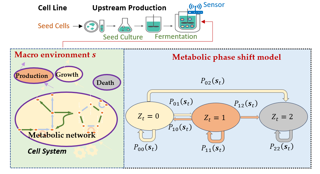
To support interpretable predictions and optimal control of biomanfuacturing processes, in this paper, we develop a digital twin calibration approach to guide a sequential design of experiments (DoEs). It can sample efficiently improve model fidelity of multi-scale bioprocess mechanistic model for Biological System-of-Systems (Bio-SoS) (Zheng et al., 2024) that characterizes the fundamental bioprocessing mechanisms and causal interdependence from molecular- to cellular- to macro-kinetics. Even though this study is motivated by cell culture process, the proposed optimal learning approach can be extended to calibrate the digital twin of general Bio-SoS with modular design. In specific, the dynamics and variations of cell culture process is characterized by a multi-scale mechanistic model composed of sub-modules or modules: (1) a single cell mechanistic model characterizing each living cell behaviors and their interactions with environment; (2) a metabolic shift model characterizing the change of cell metabolic phase and behaviors as a response to culture condition changes and cell age; and (3) macro-kinetic model of a bioreactor system composed of many living cells under different metabolic phases.
The benefits of considering the Bio-SoS mechanistic model with modular design include: a) support flexible manufacturing through assembling a system of modules to account for biomanufacturing processes under different conditions and with various inputs; and b) facilitate the integration of experimental data from different production systems, such as 2D culture and 3D culture for Induced pluripotent stem cell (iPSCs). By accounting for the structure property of the Bio-SoS mechanistic model, we can quantify how the model uncertainties or estimation errors of different modules interact with each other and propagate through the reaction mechanism pathways to outputs, which can support the interpretable design of experiments to enhance model fidelity and improve predictions.
Before describing the proposed calibration approach, we review the key aspects for digital twin calibration. First, the model uncertainty quantification approaches for digital twins and simulators can be divided into two main categories: Bayesian and frequentist approaches (Corlu et al., 2020). Bayesian approaches treat unknown model parameters as random variables and quantify our belief by using posterior distributions. It involves specifying prior distributions for model parameters and updating these distributions based on the information collected from observed data by applying Bayes’ theorem. On the other hand, frequentist approaches estimate model parameters using traditional statistical methods, such as maximum likelihood estimation, to find parameter values that maximize the likelihood of observed data. The model estimation uncertainty can be quantified by asymptotic normal approximation or bootstrap approach. These frequentist estimation approaches could be easier and faster compared with Bayesian inference approaches since there may not exist conjugate priors and posterior sampling update can be computationally expensive.
Second, for the propagation of input and model uncertainty to simulation outputs, to save computational budget and time, a metamodel is often used to approximate the response surface, especially for complex stochastic systems, since easy experiment can be expensive. In the classical calibration approach (Kennedy and O’Hagan, 2001), the Gaussian processes (GPs) are used to characterize the mean response and model discrepancies. Although GP metamodel is often used to propagate the input to output and further support the digital twin calibration, it’s hard to interpret and difficult to leverage prior knowledge of the real biomanufacturing system mechanisms. To enhance interpretability and sample efficiency, the mechanistic models can be employed to construct the response surface in our study.
Third, the selection of calibration criteria plays a critical role to guide the experiments and most informative data collection to improve model fidelity and support digital twin calibration. The existing calibration approaches often focus on system design. Mean response and Mean Squared Error (MSE) are widely used as a criteria for assessing model prediction accuracy. Tuo and Jeff Wu (2016) shows Kennedy’s method, which models the mean output as a GP, may lead to asymptotically -inconsistent. They modify the criteria into norm of the discrepancy between real and digital system outputs and propose a -consistent calibration method, which can ensure an optimal convergence rate.
To support process control and facilitate biomanufacturing process automation, in this paper, we aim to calibrate the Bio-SoS mechanistic model to guide a sequential DoE and improve model fidelity and prediction accuracy of digital twin. We first employ the Maximum Likelihood Estimation (MLE) method to estimate model parameters and utilize bootstrap techniques to quantify estimation uncertainty across different modules. Then, to optimize the digital twin calibration policy that will be used to sequentially guide the experiments and the most informative data collection, we derive the gradient of prediction MSE and use the steepest descent to efficiently search for the optimal policy parameters, which makes the learning process more interpretable. Since it is challenging to find a closed form solution of the mechanistic model with stochastic differential equations (SDEs) form, we utilize the linear noise approximation (LNA) for uncertainty propagation and constructs a surrogate model for MSE. Thus, in an online setting, a calibration policy is iteratively updated by using a stochastic gradient method where the gradient of MSE with respect to the calibration policy parameter follows the backward direction of the uncertainty propagation. The proposed calibration approach accounts for the Bio-SoS mechanism structure. That means it quantifies Bio-SoS module error interaction and their propagation through mechanistic pathways to output, which guides the sequential design of experiments to efficiently improve model fidelity and prediction accuracy.
In sum, we develop an interpretable and sample efficient optimal learning approach to support digital twin calibration for a multi-scale bio-process mechanistic model so that the digital twin of the cell culture process can improve process prediction and support optimal control. Even though this paper focuses on cell culture, the proposed calibration approach can be extendable to general biomanufacturing systems. The key contributions of the proposed calibration approach and the benefits are summarized as follows.
-
•
We proposed a new DoE method for calibrating a multi-scale bioprocess mechanistic model by updating the parameters using closed-form gradients that incorporate the mechanistic information.
-
•
We assess the MSE of the process output prediction and use a LNA-based metamodel along with Euler’s method to estimate how model uncertainty propagates through Bio-SoS mechanism pathways and impacts on the output prediction accuracy. This approach can advance our understanding on how the errors in individual module parameters affect the overall prediction accuracy of digital twin model.
-
•
Built on the LNA, we further develop a gradient-based policy optimization to guide most informative experiments and support sample-efficient optimal learning.
The organization of the paper is as follows. In Section 2, we describe the multi-scale mechanistic model. Then, we propose the novel calibration method for the multi-scale model in Sections 3, which includes two main procedures: model inference and policy update. A stochastic gradient method is developed for the model inference in Section 4. The calibration policy gradient estimation and update method is further developed in Section 5. Then we empirically validate the proposed digital twin calibration approach in Section 6 and conclude this paper in Section 7.
2 Problem Description and Bio-SoS Mechanistic Model
In this study, we explore a multi-scale bioprocess mechanistic model designed to elucidate the interdependencies that exist across molecular, cellular, and macroscopic levels within cell culture processes. This comprehensive model integrates the complexities of biological interactions within and between these scales and extends applicably to a broader range of biological systems, referred to as Biological System-of-Systems (Bio-SoS). A detailed summary of the variable notations used within our model is provided in Table 1.
The core of our model is based on the structured Markov chain, capturing both the dynamics and variability inherent in cellular processes through a state transition probabilistic model. Conceptually, each individual cell operates as a complex system, and collectively, numerous cells at various metabolic phases within the bioreactor form an intricate system of systems. This interaction is depicted in Figure 1, where, for clarity, only three distinct metabolic phases are illustrated. Cells interact with each other by altering their environment, notably through nutrient uptake and the production of metabolic wastes, and in turn, respond to these environmental changes.
| Single cell state | Macro-state | ||
| Reaction indices () | Cell phases for single cell () | ||
| Cell density in -th phase () | State component indices () | ||
| Time () | Calibration iteration number () | ||
| Transition probability from - to -th phase | Parameters for phase shift model | ||
| Model parameters for cells in phase | True model parameters | ||
| Estimated model parameters at iteration | Policy parameters | ||
| Learning rate for updating parameter | Learning rate for updating policy | ||
| Virtual model update function | bootstrapping estimation for |
At any time , for each single cell in the -th metabolic phase, denoted by with (i.e., growth, stationary, death phases, etc), the dynamic behaviors of its metabolic network can be characterized by a stochastic model specified by parameters . The regulation mechanism and reaction rate of metabolic network respond to the change of environmental condition is denoted by . The metabolic phase shift model with represents the transition probability from to . Therefore, in this paper, we focus on calibrating the mechanistic model of the Bio-SoS specified by the calibration parameters : (1) characterizing cell dynamics in -th metabolic phase or class; and (2) characterizing the phase shift probability that impacts the percentage of cells in each phase or class.
2.1 Single Cell Model
This section briefly describes a stochastic metabolic model characterizing the dynamics of a single cell across different metabolic phases: growth (), production () and so on. The model includes two main components: the Stochastic Modular Reaction Networks (SMRN) and the metabolic phase shift dynamics. Following the study (Anderson and Kurtz, 2011), the SMRN can be constructed
| (1) |
where is the state for cells in -th phase, represents the stoichiometric matrix characterizing the structure of molecular reaction network, and follows a multivariate Poisson process with molecular reaction rate vector . This reaction rate depends on macro-environment , typically modeled by using a Michaelis-Menten (MM) kinetic equation (Kyriakopoulos et al., 2018; Wang et al., 2024).
The second component on metabolic shift model addresses the transitions between metabolic phases in response to environmental changes. At any time , we have the metabolic phase-shift probability matrix depending on the environmental condition , where each element represents
2.2 Macro-Kinetic State Transition
Suppose the environmental condition in bioreactor is homogeneous over space. The cell population dynamics are characterized by the evolution of cell densities in each metabolic phase , i.e.
| (2) |
where represents growth rate characterizing the growth of the cell population and the second term counts the cells metabolic shifting from -th phase to -th phase.
Let denote metabolite concentrations (i.e., the number of molecules per unit of volume) in the system at time . Let represent the change in metabolic concentration for the -th cell in phase . Then at any time , given the density of cells located in phase , the overall change of metabolite concentration is the sum of the contributions from individual cells,
| (3) |
where is a multivariate Poisson process with reaction rate vector ; as detailed in Eq. (10) from Zheng et al. (2024). Without losing generality, in the following sections, we consider a two-phase mechanistic model with parameters .
2.3 State Transition Probability
In an infinitesimal time change , the change of state becomes,
where is a multivariate Poisson process with parameter . Then and , with representing the component indices of . The approximation is made under the assumption that the time interval is small, so the state doesn’t change too much and different reactions can be treated independent. By forming as a Stochastic Differential Equations (SDEs), we have
| (4) |
where denotes standard Brownian motion. It is hard to find the analytic solution to (4), so we take an approximation in a short time interval , i.e.,
where is a Gaussian random vector with mean zero and covariance matrix . Finally, we approximate conditional distribution of as
| (5) |
where , .
3 Digital Twin Calibration for Bio-SoS Mechanistic Model
To facilitate the mechanistic model digital twin calibration, in this paper, we consider the physical system as a finite horizon stochastic process. Its dynamics can be characterized by a Bio-SoS mechanistic model specified by Eq. (2) and (3) with underlying true parameters, denoted by . Our goal is to develop an optimal learning calibration approach that can efficiently guide the sequential design of experiments and most informative data collection to improve model fidelity and the prediction accuracy of the digital twin. For simplification, we consider batch-based cell culture experiments with the selection of initial concentration as the decision variable.
The trajectory over a horizon of time steps has the joint probability density function
| (6) |
where is a deterministic design or calibration policy parameterized by . Each transition probability follows a normal distribution as defined in Eq. (5).
At each -th calibration iteration, we select one design following the latest policy, i.e. , run an experiment to collect one sample path from the physical system, and then update the parameter . Specifically, given the historical samples , we consider maximizing the log-likelihood for model parameters , i.e.,
| (7) |
where denotes the sum of log-likelihoods and is the log-likelihood of trajectory with initial state . The detailed derivation can be found in Section 4.
For digital twin calibration, we select the design of new experiment at the beginning of -th iteration. This selection is based on the evaluation of our current model on a pre-specified set of evaluation and prediction points . The objective is to minimize the MSE of digital twin prediction,
| (8) |
where denote the virtual model update function with the simulated trajectory (see Eq. (10)) and represents the system outputs of interest, such as yield and product quality attributes. The superscript "p" indicates the output from the physical system and "d" for digital twin.
To sample efficiently guide digital twin calibration, we propose a gradient-based optimal learning approach with the procedure illustration as shown in Figure 2 and develop a calibration algorithm summarized in Algorithm 1. In specific, for the optimization problem (7) , we use the gradient-based method to search for the MLE, i.e.,
| (9) |
where “Adam” represents Adam optimizer (Kingma and Ba, 2014). The details of the optimization steps will be discussed in section 4. Now we can define virtual model update function
| (10) |
with a simulated trajectory and . Then to guide informative experiment and improve digital twin prediction, we solve the optimization (8) by using the stochastic gradient descent
| (11) |
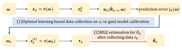
Inspired by Figure 2, we compute the gradient with respect to using the chain rule. Specifically, we take the gradient with respect to , and then take the gradient to with respect to , i.e.,
| (12) |
Since is unknown, we use the bootstrapping to quantify the model parameter estimation uncertainty in Section 5. Following the upper part of Figure 2, the prediction error propagates from to model parameter update , and then to our objective . By taking the gradient of , we can discern the influence of the experimental design specified by on the final prediction error, which assists in selecting a more effective design. Since deriving an exact expression for this gradient is complex, we develop a linear noise approximation closed-form representation, which will be detailed in Section 5. This approximation provides an efficient method for improving calibration policy.
-
1.
Compute by Eq. (10)
4 Model Inference and Parameter Update
The gradient of the log-likelihood is calculated as
Each term in this summation involves gradients that are detailed in the following lemma.
Lemma 1.
Conditioning on the current state and model parameter , the state change during in any small time interval is following a multi-variate normal distribution . Then the gradient of log-likelihood with respect to is given by
Proof.
By the definition of multi-variant normal distribution, we have
Taking the logarithm on both side, we have
The gradient for the first term is where is a tensor of with as the length of , and "tr" represents the trace for first two dimensions. The gradient for the second term is
∎
Given the calculated gradient, we can use the Adam optimizer Kingma and Ba (2014) for updating . Following the algorithm in their paper, for the -th iteration, we have
| (13) |
where is the learning rate, is the gradient of the likelihood function at -th iteration, is the element-wise square, are hyper-parameters related to exponential decay rates, is a small number to avoid zero in the denominator.
5 Policy Gradient Estimation and Optimal Learning
In this section, we turn our focus on learning the calibration policy by minimizing the prediction MSE in (8). To develop a surrogate model of this MSE, we employ the linear noise approximation in Section 5.1 to approximate the stochastic dynamics of the system and the solution of SDE-based mechanistic model, reflecting its sensitivity to initial conditions and parameter values. This approach allows us to describe the system state at any given time as a normally distributed random variable, facilitating the derivation of analytical expressions for the gradient estimator. To keep the mechanism information, in Section 5.2, a first-order Euler’s Method is utilized to derive the closed-form solutions of the SDEs based mechanisms obtained from linear noise approximation.
5.1 Linear Noise Approximation on Bio-SoS Dynamics
We use linear noise approximation (LNA) (Fearnhead et al., 2014) to derive the solution of SDEs as shown in Lemma 2 that allows us to analyze the estimation error propagation from to the output prediction and develop a surrogate model of the MSE (8). Conditional on and , we denote the state of systems at time as . Considering the SDEs characterizing the Bio-SoS dynamics as shown in (4), we have
| (14) |
where and
Lemma 2.
(Linear Noise Approximation) Suppose , and . Then the solution of SDE (14) can be approximated as
where are the solution of ordinary differential equations (ODEs)
| (15) |
where we assume with representing the deterministic path and representing stochastic path, is the matrix with components
Proof.
Proof can be find in Fearnhead et al. (2014) with . ∎
Obtaining an analytical solution for the series of ODEs described in (15) is challenging. Therefore, we use a numerical solution approach, as described in Section 5.2. This method involves applying the solution iteratively at each time step , allowing us to approximate the system’s behavior over time. For the physical system and digital twin, we denote
Then we have For any -th component , we have a surrogate model of the MSE (8)
| (16) |
5.2 First-Order Euler’s Method for Solving LNA
To get the solution of , we solve the ODEs outlined in (15) numerically by using first-order Euler’s method. For the term , the update equation is given by
| (17) |
For the term , the update equation is given by
| (18) |
Then by (16)-(18), the final output discrepancy can be written as
Then conditional on , by applying a chain rule, we can update the policy parameters by
| (19) |
where and . Here is a gradient based on simulation trajectory since is updated at the beginning of -th iteration and we can not get physical data .
To quantify the estimation error of underlying true model parameters , we use the parametric bootstrapping. Based on MLE and data , we have as the estimator for . Then we can generate bootstrap samples, denoted as , . Then we can take the following estimation
6 Empirical Study
To assess the performance of the proposed calibration approach, we employ a simpler version of the Chinese Hamster Ovary (CHO) cell culture model as described by Ghorbaniaghdam et al. (2014) as our SMRN model. We use this model with a state shift model to simulate cell culture dynamics and compare our gradient-based policy against a random policy for a DoE problem. We detail the model and its validation in Section 6.1, and present the comparative results in Section 6.2.
6.1 Cell Culture Model and Validation
CHO cells have become the most commonly used mammalian hosts for industrial production of monoclonal antibodies (mAbs) and recombinant protein therapeutics. This is due to their capacity to correctly fold, assemble, and modify human proteins, ensuring biological activity and stability. The robustness of CHO cells, coupled with their genetic and metabolic malleability, makes them ideal candidates for genetic engineering and optimization for specific production processes. The cell growth model is described by a function characterizing different phases of cell culture
where represents the growth rate that depends on glucose concentration in the growth phase (phase 0) and where and are phase transition rates, reflecting the dynamic interplay between growth and production phases. A simplified SMRN focuses on three key metabolisms: glucose consumption, lactate production, and monoclonal antibody synthesis with chemical equations
where GLC, LAC and mAb represent glucose, lactate and monoclonal antibodies. The state of the system at any time is denoted by representing the concentrations of glucose, lactate, and mAb, respectively. The flux rates , where denotes the rate of glucose consumption, represents the stoichiometric production of lactate , and quantifies the mAb production rate. The kinetic equations of two phases are described as
The metabolic reactions are formulated as a SDE system (14) to account for the inherent randomness and fluctuations in biochemical reactions. The general form of this SDE is given by
where the mean function is modeled by the stoichiometric matrix
and reaction rates . The system variability is modeled by .
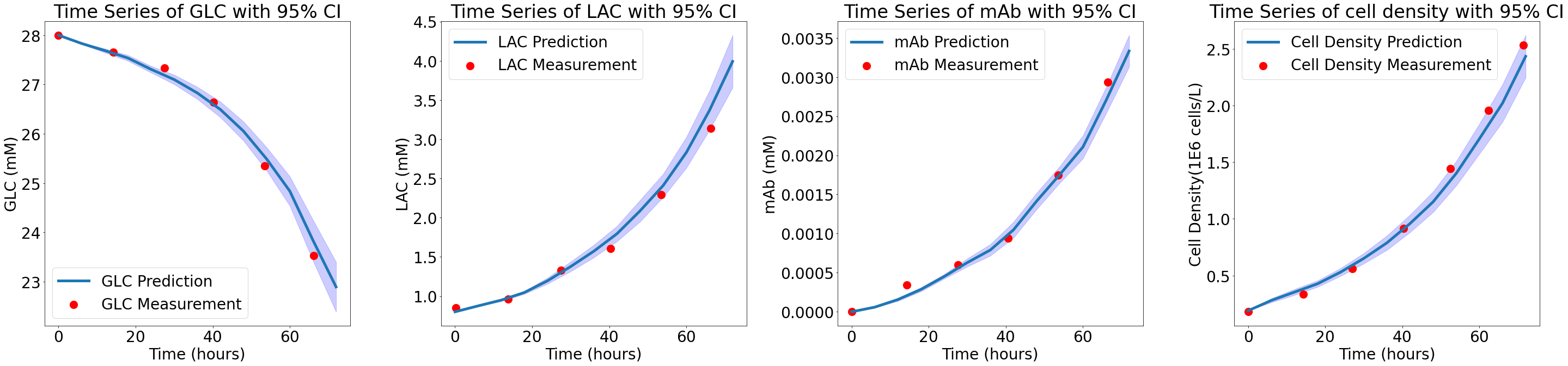
We fit our model by minimizing between experiment data from Ghorbaniaghdam et al. (2014) and simulation model prediction . The results of our model validation are depicted in Figure 3. The figure presents experimental data as red dots and the simulation results as blue lines, which illustrate both the mean and the 95% confidence interval (CI) of the model predictions. The CI is calculated by the formula , where is the sample mean, is the z-score corresponding to the 95% confidence level, which is approximately 1.96, is the standard deviation of the sample, is the number of observations in the sample. This result shows the model’s effectiveness in capturing the dynamics of the CHO cell culture system.
In the empirical study assessing the performance of the proposed calibration approach, we use the fitted parameters as the true model parameters of the physical system, i.e.,
| (20) | ||||
| (21) | ||||
| (22) |
and assume the digital twin has the same model structure with unknown parameters.
6.2 Digital Twin Calibration
With the true parameters defined in (20) to (22), our objective is to calibrate the digital twin model by strategically designing CHO cell culture experiments. The aim is to minimize the model prediction error by choosing the initial glucose concentration as design decision variable. In each experiment, we adjust the initial glucose concentration and then collect a new batch of data to sequentially refine our model.
For the calibration experiments setting, we assume time course data of the states is collected every 12h until 72h, so each batch includes 7-time sequence data. We focus on calibrating parameters . The design space for the initial concentrations of glucose is set within the range mM, and the initial concentration of lactate and mAb are mM, mM, the initial cell densities in Phase 0 and 1 are set to be cells/L, cells/L, respectively. The initial parameters for the digital twin are estimated based on the first batch of data. Since the model parameters are in different scales, we set a learning rate for updating the calibrating parameters and for updating the design policy by applying Eq. (19). The fixed set of test data is composed of initial states and .
We conducted 15 macro-replications, each consisting of iterations under varying initial conditions, with initial glucose levels randomly chosen by applying the uniform distribution over the interval . We compare the proposed gradient-based calibration approach with a random design approach, where the design is uniformly sampled from . To ensure consistency across the two approaches, we used the same random seeds for these two approaches. The mean prediction performance and the 95% confidence interval, calculated across macro-replications, represented by the Mean Relative Errors with script representing the -th component, are presented in Figure 5 for mAb prediction and in Figure 5 for parameter estimation, respectively. For both figures, blue lines represent the performance of our approach, while yellow lines represent the random design performance.
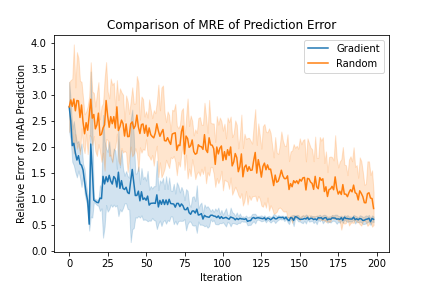
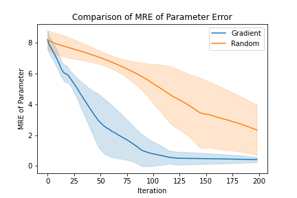
The results demonstrate that the proposed Bio-SoS model calibration approach is significantly more sample-efficient than a random design. After 125 iterations, MRE for mAb production predictions using our calibration approach is reduced to approximately 60%, in contrast to roughly 200% for predictions made through random design. Furthermore, the MRE for parameters using our approach decreases to around 30% after 125 iterations, whereas the MRE for the random policy stays as high as 400%.
7 CONCLUSION
This study develops a robust digital twin calibration approach for a Bio-SoS mechanistic model in the context of cell culture processes. By strategically guiding more informative data collection through the proposed gradient-based calibration approach, we significantly enhance the model fidelity and predictive accuracy of the digital twin. The empirical validation using the CHO cell culture model underscores the superiority of our approach over the traditional random design, showcasing its potential applicability across various biological systems. Overall, this study not only contributes to the theoretical advancements in bioprocess digital twin development but also holds promise for practical implementations that could improve the efficiency and effectiveness of biomanufacturing in the pharmaceutical industry.
References
- Zheng et al. [2024] Hua Zheng, Sarah Harcum, Jinxiang Pei, and Wei Xie. Stochastic biological system-of-systems modelling for ipsc culture. Communications Biology, 7, 01 2024. doi:10.1038/s42003-023-05653-w.
- Corlu et al. [2020] Canan G. Corlu, Alp Akcay, and Wei Xie. Stochastic simulation under input uncertainty: A review. Operations Research Perspectives, 7:100162, 2020. ISSN 2214-7160. doi:https://doi.org/10.1016/j.orp.2020.100162. URL https://www.sciencedirect.com/science/article/pii/S221471602030052X.
- Kennedy and O’Hagan [2001] Marc C. Kennedy and Anthony O’Hagan. Bayesian calibration of computer models. Journal of the Royal Statistical Society: Series B (Statistical Methodology), 63(3):425–464, 2001. doi:https://doi.org/10.1111/1467-9868.00294. URL https://rss.onlinelibrary.wiley.com/doi/abs/10.1111/1467-9868.00294.
- Tuo and Jeff Wu [2016] Rui Tuo and C. F. Jeff Wu. A theoretical framework for calibration in computer models: Parametrization, estimation and convergence properties. SIAM/ASA Journal on Uncertainty Quantification, 4(1):767–795, 2016. doi:10.1137/151005841. URL https://doi.org/10.1137/151005841.
- Anderson and Kurtz [2011] David F. Anderson and Thomas G. Kurtz. Continuous Time Markov Chain Models for Chemical Reaction Networks, pages 3–42. Springer New York, New York, NY, 2011. ISBN 978-1-4419-6766-4. doi:10.1007/978-1-4419-6766-4_1. URL https://doi.org/10.1007/978-1-4419-6766-4_1.
- Kyriakopoulos et al. [2018] Sarantos Kyriakopoulos, Kok Siong Ang, Meiyappan Lakshmanan, Zhuangrong Huang, Seongkyu Yoon, Rudiyanto Gunawan, and Dong-Yup Lee. Kinetic modeling of mammalian cell culture bioprocessing: The quest to advance biomanufacturing. Biotechnology Journal, 13(3):1700229, 2018. doi:https://doi.org/10.1002/biot.201700229. URL https://analyticalsciencejournals.onlinelibrary.wiley.com/doi/abs/10.1002/biot.201700229.
- Wang et al. [2024] Keqi Wang, Wei Xie, and Sarah W. Harcum. Metabolic regulatory network kinetic modeling with multiple isotopic tracers for ipscs. Biotechnology and Bioengineering, 121(4):1335–1353, 2024. doi:https://doi.org/10.1002/bit.28609. URL https://analyticalsciencejournals.onlinelibrary.wiley.com/doi/abs/10.1002/bit.28609.
- Kingma and Ba [2014] Diederik Kingma and Jimmy Ba. Adam: A method for stochastic optimization. International Conference on Learning Representations, 2014.
- Fearnhead et al. [2014] Paul Fearnhead, Vasilieos Giagos, and Chris Sherlock. Inference for reaction networks using the linear noise approximation. Biometrics, 70(2):457–466, 2014. doi:https://doi.org/10.1111/biom.12152. URL https://onlinelibrary.wiley.com/doi/abs/10.1111/biom.12152.
- Ghorbaniaghdam et al. [2014] Atefeh Ghorbaniaghdam, Jingkui Chen, Olivier Henry, and Mario Jolicoeur. Analyzing clonal variation of monoclonal antibody-producing cho cell lines using an in silico metabolomic platform. PLOS ONE, 9, 2014. URL https://api.semanticscholar.org/CorpusID:5913733.