Approximating a branch of solutions to the Navier–Stokes equations by reduced-order modeling

Abstract

This paper extends a low-rank tensor decomposition (LRTD) reduced order model (ROM) methodology to simulate viscous flows and in particular to predict a smooth branch of solutions for the incompressible Navier-Stokes equations. Additionally, it enhances the LRTD-ROM methodology by introducing a non-interpolatory variant, which demonstrates improved accuracy compared to the interpolatory method utilized in previous LRTD-ROM studies. After presenting the interpolatory and non-interpolatory LRTD-ROM, we demonstrate that with snapshots from a few different viscosities, the proposed method is able to accurately predict flow statistics in the Reynolds number range $[25,400]$. This is a significantly wider and higher range than state of the art (and similar size) ROMs built for use on varying Reynolds number have been successful on. The paper also discusses how LRTD may offer new insights into the properties of parametric solutions.

1 Introduction

We are interested in reduced order modeling of the incompressible Navier-Stokes equations (NSE), which are given by

(1) $$\left\{\begin{aligned} \frac{\partial\mathbf{u}}{\partial t}+(\mathbf{u}\cdot\nabla)\mathbf{u}-\nu\Delta\mathbf{u}+\nabla p&=0,\\ \mbox{div}\mathbf{u}&=0,\end{aligned}\right.$$

in a bounded Lipschitz domain $\Omega$ and for $t\in(0,T)$ with a final time $T>0$, and suitable initial and boundary conditions. Here $\mathbf{u}$ and $p$ are the unknown fluid velocity and pressure, and $\nu>0$ is the kinematic viscosity. We treat $\nu$ as a positive constant parameter that can take values from the range $[\nu_{\min},\nu_{\max}]$. The problem addressed in the paper consists of an effective prediction of flow statistics for the entire range $[\nu_{\min},\nu_{\max}]$, based on the information learned from a set of flow states $\mathbf{u}(t^{n},\nu^{k}),\,p(t^{n},\nu^{k})$ (further called snapshots) computed for a finite sample of parameters (training set) $\mathcal{A}=\{\nu^{k}\}_{k=1}^{K}\subset[\nu_{\min},\nu_{\max}]$ at given time instances $\{t^{n}\}_{n=1}^{N}\subset(0,T]$.

Assuming $\mathbf{u},p$ depends smoothly on $\nu$, the problem outlined above can be, of course, addressed by numerically solving (1) for a sufficiently dense sample $\mathcal{A}$ and proceeding with interpolation. This strategy, however, may entail prohibitive computational costs of solving the full order model multiple times for a large set of parameters and impractical data storage. Furthermore, for long-time simulations, such an interpolation strategy may fail to be sustainable given that solution trajectories may (locally) diverge exponentially fast (although in 2D the system has a finite dimensional attractor [5] which could be captured by a ROM).

For a fast and accurate computations of flow statistics for any $\nu\in[\nu_{\min},\nu_{\max}]$, the present paper considers a reduced order model (ROM) which uses a low-rank tensor decomposition (LRTD) in the space–time–parameter space as the core dimension reduction technique. As such, LRTD replaces SVD/POD, the standard reduction method in more traditional POD–ROMs. This allows for the recovery of information about the parameter-dependence of reduced spaces from a smaller set of pre-computed snapshots and to exploit this information for building parameter-specific ROMs. The LRTD–ROM was recently introduced in [18] and further developed and analyzed in [19, 20].

This is the first time LRTD–ROM is applied to the system (1) and, more generally, to predict the dynamics of a viscous fluid flow. The paper extends the approach to the parameterized incompressible Navier–Stokes equations. We introduce a non-interpolatory variant of LRTD–ROM. The method is applied to predict drag and lift coefficients for a 2D flow passing a cylinder at Reynolds numbers $\text{Re}\in[25,400]$. This branch of solutions contains the first bifurcation point at around $\text{Re}=50$ [4, 27], when the steady state flow yields to an unsteady periodic flow.

Predicting flow dynamics along a parameterized branch of solutions is a challenging task for traditional ROMs, since building a universal low-dimensional space for a range of parameter(s) may be computationally expensive if possible at all. Recent studies that develop or apply reduced order modeling to parameterized fluid problems include [16, 22, 13, 13, 23]. In particular, several papers addressed the very problem of applying ROMs to predict a flow passing a 2D cylinder for varying Re number. The authors of [8] applied dynamic mode decomposition (DMD) with interpolation between pre-computed solutions for 16 values of viscosity to predict flow for $\text{Re}\in[85,100]$. In [1] the DMD with 14 viscosity values in the training set was applied to forecast the flow around the first bifurcation point $R=50$ (the actual Re numbers are not specified in the paper). A stabilized POD–ROM was tested in [25] to predict the same flow for $\text{Re}\in[100,200]$. In [10] the same problem of the 2D flow around a circular cylinder for varying Re numbers was approached with a POD–ROM based on greedy sampling of the parameter domain. Such POD–ROM required then offline computations of FOM solutions for 51 values of Re to predict flow statistics for $\text{Re}\in[75,100]$. Compared to these studies, the LRTD–ROM is able to handle significantly larger parameter variations with nearly the same or smaller training sets. For example, we found 13 values of Re log-uniformly sampled to be sufficient for LRTD–ROM with reduced dimension of 20 to reasonably predict the same flow statistics for $\text{Re}\in[25,400]$. This exemplifies the prediction capability of LRTD based projection ROM for fluid problems.

The remainder of the paper is organized as follows. Section 2 describes the FOM, which is a second-order in time Scott-Vogelius finite element method on a sequence of barycenter refined triangulations. Section 3 introduces the reduced order model. In section 4 the model is applied to predict the 2D flow along a smooth branch of solutions.

2 Full order model

To define a full order model for our problem of interest, we consider a conforming finite element Galerkin method: Denote by $\mathbf{V}_{h}\subset H^{1}(\Omega)^{d}$ and $Q_{h}\subset L^{2}_{0}(\Omega)$ velocity and pressure finite element spaces with respect to a regular triangulation $\mathcal{T}_{h}$ of $\Omega$. For $\mathbf{V}_{h}$ and $Q_{h}$ we choose the lowest order Scott-Vogelius finite element pair:

(2) $$\begin{split}\mathbf{V}_{h}&=\{\mathbf{v}\in C(\Omega)^{2}:\,\mathbf{v}\in\left[\mathbb{P}_{2}(T)\right]^{2}~{}\forall\,T\in\mathcal{T}_{h}\},\\ Q_{h}&=\{q\in L^{2}(\Omega):\,q\in\mathbb{P}_{1}(T)~{}~{}~{}~{}\forall\,T\in\mathcal{T}_{h}\}.\end{split}$$

The lowest order Scott-Vogelius (SV) element is known [2] to be LBB stable in 2D on barycenter refined meshes (also sometimes referred to as Alfeld split meshes). Hence we consider $\mathcal{T}_{h}$ such that it is obtained by one step of barycenter refinement applied to a coarser triangulation. Since $\mbox{div}(\mathbf{V}_{h})\subseteq Q_{h}$, it is an example of a stable element which enforces the divergence free constraint for the finite element velocity pointwise.

Denote by $I_{h}(\cdot)$ any suitable interpolation operator of velocity boundary values. We use $(f,g):=\int_{\Omega}f\cdot g\,dx$ notation for both scalar and vector functions $f,g$. We also adopt the notation $\mathbf{u}_{h}^{n}$ and $p_{h}^{n}$ for the finite element approximations of velocity and pressure at time $t_{n}=n\Delta t$, with $\Delta t=T/N$ and $n=0,1,2,\dots,N$.

The second order in time FE Galerkin formulation of (1) with $\mathbf{u}={\bf g}$ on $\partial\Omega$ reads: Find $\mathbf{u}_{h}^{n}\in\mathbf{V}_{h}$, $\mathbf{u}_{h}^{n}=I_{h}(\mathbf{g}(t_{n}))$ on $\partial\Omega$ and $p_{h}^{n}\in Q_{h}\cap L^{2}_{0}(\Omega)$, for $n=1,2,\dots,N$, such that satisfying

(3) $$\Big{(}\frac{3\mathbf{u}_{h}^{n}-4\mathbf{u}_{h}^{n-1}+\mathbf{u}_{h}^{n-2}}{2\Delta t},\mathbf{v}_{h}\Big{)}+((2\mathbf{u}_{h}^{n-1}-\mathbf{u}_{h}^{n-2})\cdot\nabla\mathbf{u}_{h}^{n},\mathbf{v}_{h})\\ +\nu(\nabla\mathbf{u}_{h}^{n},\nabla\mathbf{v}_{h})-(p_{h}^{n},\mbox{div}\mathbf{v}_{h})+(\mbox{div}\mathbf{u}_{h}^{n},q_{h})=0,$$

for all $\mathbf{v}_{h}\in\mathbf{V}_{h}$, s.t. $\mathbf{v}_{h}={\bf 0}$ on $\partial\Omega$, $q_{h}\in Q_{h}$, and $\mathbf{u}_{h}^{0}=\mathbf{u}(0)$. The first step for $n=1$ is done by the first order implicit Euler method.

The stability and convergence of the method can be analyzed following textbook arguments (e.g. [9, 7]), implying the estimate

(4) $$\max_{n=1,\dots,N}\|\mathbf{u}^{n}_{h}-\mathbf{u}(t^{n})\|^{2}_{L^{2}(\Omega)}+\Delta t\nu\sum_{n=1}^{N}\|\nabla(\mathbf{u}^{n}_{h}-\mathbf{u}(t^{n}))\|^{2}_{L^{2}(\Omega)}\leq C(\mathbf{u},p,\nu)(|\Delta t|^{4}+h^{4}),$$

where $h=\max_{T\in\mathcal{T}_{h}}\text{diam}(T)$, and $C(\mathbf{u},p,\nu)$ is independent on the mesh parameters but depends on the regularity (smoothness) of $\mathbf{u}$ and $p$. Under extra regularity assumptions, the optimal order velocity and pressure estimates follow in the $L^{\infty}(L^{2})$-norms [14]:

(5) $$\max_{n=1,\dots,N}(\|\mathbf{u}^{n}_{h}-\mathbf{u}(t^{n})\|_{L^{2}(\Omega)}+h\|p^{n}_{h}-p(t^{n})\|_{L^{2}(\Omega)})\leq C(\mathbf{u},p,\nu)(|\Delta t|^{2}+h^{3}).$$

3 Reduced order model

The LRTD–ROM is a projection based ROM, where the solution is sought in a parameter dependent low dimensional space. Since the divergence-free finite elements are used for the FOM model, the low dimensional ROM space is a velocity space $\mathbf{V}^{\ell}(\nu)\subset\mathbf{V}_{h}$, $\mbox{dim}(\mathbf{V}^{\ell}(\nu))=\ell\ll M$, such that

(6) $$\mbox{div}\mathbf{v}_{\ell}=0\quad\text{for all}~{}\mathbf{v}_{\ell}\in\mathbf{V}^{\ell}(\nu).$$

Thanks to (6), the pressure does not enter the projected equations and the reduced order model reads: Find $\mathbf{u}_{\ell}^{n}\in\mathbf{V}_{\ell}(\nu)$, for $n=1,2,\dots,N$, such that satisfy

(7) $$\Big{(}\frac{3\mathbf{u}_{\ell}^{n}-4\mathbf{u}_{\ell}^{n-1}+\mathbf{u}_{\ell}^{n-2}}{2\Delta t},\mathbf{v}_{\ell}\Big{)}+((2\mathbf{u}_{\ell}^{n-1}-\mathbf{u}_{\ell}^{n-2})\cdot\nabla\mathbf{u}_{\ell}^{n},\mathbf{v}_{\ell})+\nu(\nabla\mathbf{u}_{\ell}^{n},\nabla\mathbf{v}_{\ell})=0,$$

for all $\mathbf{v}_{\ell}\in\mathbf{V}_{\ell}(\nu)$, and $\mathbf{u}_{\ell}^{0}=\mathbf{P}_{\ell}\mathbf{u}(0)$, where $\mathbf{P}_{\ell}$ is a projector into $\mathbf{V}_{\ell}(\nu)$. Similar to the FOM, the implicit Euler method is used for $n=1$. Once the velocities $\mathbf{u}_{\ell}^{n}$ are known, the corresponding pressure functions $p_{\ell}^{n}\in Q_{h}$ can be recovered by a straightforward post-processing step, see, e.g.  [3].

The critical part of the ROM is the design of a parameter-specific low-dimensional space $\mathbf{V}_{\ell}(\nu)$. This is done within a framework of a LRTD–ROM (sometimes referred to as Tensor ROM or TROM), which replaces the matrix SVD – a traditional dimension reduction technique – by a low-rank tensor decomposition. The application of tensor technique is motivated by a natural space–time–parameters structure of the system. This opens up possibilities for the fast (online) finding of an efficient low-dimensional $\nu$-specific ROM space for arbitrary incoming viscosity parameter $\nu$. The resulting LRTD–ROM consists of (7), offline part of applying LRTD, and online part with some fast linear algebra to determine $\mathbf{V}_{\ell}(\nu)$. Further details of LRTD–ROM are provided next.

3.1 LRTD–ROM

Similar to the conventional POD, on an offline stage a representative collection of flow velocity states, referred to as snapshots, is computed at times $t_{j}$ and for pre-selected values of the viscosity parameter:

$$\mathbf{u}_{h}(t_{j},\nu_{k})\in\mathbf{V}_{h},\quad j=1,\ldots,N,\quad k=1,\ldots,K.$$

Here $\mathbf{u}_{h}$ are solutions of the full order model (3) for a set of $K$ viscosity parameters $\nu_{k}\in[\nu_{\min},\nu_{\max}]$.

A standard POD dimension reduction consists then in finding a subspace $\mathbf{V}^{\rm pod}_{\ell}\subset\mathbf{V}_{h}$ that approximates the space spanned by all observed snapshots in the best possible way (subject to the choice of the norm). This way, the POD reduced order space captures cumulative information regarding the snapshots’ dependence on the viscosity parameter. Lacking parameter specificity, $\mathbf{V}^{\rm pod}_{\ell}$ and so POD–ROM may lack robustness for parameter values outside the sampling set and may necessitate $\ell$ and $K$ to be large to accurately represent the whole branch of solutions. This limitation motivates the application of a tensor technique based on low-rank tensor decomposition to preserve information about parameter dependence in reduced-order spaces.

Denote by the upright symbol $\mathrm{u}^{j}(\nu)\in\mathbb{R}^{M}$ the vector of representation for $\mathbf{u}_{h}(t_{j},\nu)$ in the nodal basis. Recalling that the POD basis can be defined from the low-rank approximation (given by a truncated SVD) of the snapshot matrix, one can interpret LRTD as a multi-linear extension of POD: Instead of arranging snapshots in a matrix $\Phi_{\rm pod}$, one seeks to exploit the tensor structure of the snapshots domain and to utilize the LRTD instead of the matrix SVD for solving a tensor analogue of the low-rank approximation problem.

For LRTD–ROM, the coefficient vectors of velocity snapshots are organized in the multi-dimensional array

(8) $$(\boldsymbol{\Phi})_{:,k,j}=\mathrm{u}^{j}(\nu_{k}),$$

which is a 3D tensor of size $M\times K\times N$. The first and the last indices of $\boldsymbol{\Phi}$ correspond to the spatial and temporal dimensions, respectively.

Unfolding of $\boldsymbol{\Phi}$ along its first mode into a $M\times NK$ matrix and proceeding with its truncated SVD constitutes the traditional POD approach. In the tensor ROM the truncated SVD of the unfolded matrix is replaced with a truncated LRTD of $\boldsymbol{\Phi}$.

Although the concept of tensor rank is somewhat ambiguous, there is an extensive literature addressing the issue of defining tensor rank(s) and LRTD; see e.g. [11]. In [18, 20], the tensor ROM has been introduced for three common rank-revealing tensor formats: canonical polyadic, Tucker, and tensor train. The LRTD in any of these formats can be seen as an extension of the SVD to multi-dimensional arrays. While each format has its distinct numerical and compression properties and would be suitable, we use Tucker for the purpose of this paper.

We note that the LRTD approach is effectively applicable for multi-parameter problems. In case of a higher parameter space dimension one may prefer a hierarchical Tucker format [12] such as tensor train to avoid exponential growth of LRTD complexity with respect to the parameter space dimension.

In the Tucker format  [26, 17] one represents $\boldsymbol{\Phi}$ by the following sum of direct products of three vectors:

(9) $$\boldsymbol{\Phi}\approx\widetilde{\boldsymbol{\Phi}}=\sum_{m=1}^{\widetilde{M}}\sum_{k=1}^{\widetilde{K}}\sum_{n=1}^{\widetilde{N}}(\mathbf{C})_{m,k,n}\mathbf{w}^{m}\otimes\boldsymbol{\sigma}^{k}\otimes\mathbf{v}^{n},$$

with $\mathbf{w}^{m}\in\mathbb{R}^{M}$, $\boldsymbol{\sigma}^{k}\in\mathbb{R}^{K}$, and $\mathbf{v}^{n}\in\mathbb{R}^{N}$. Here $\otimes$ denotes the outer vector product. The numbers $\widetilde{M}$, $\widetilde{K}$, and $\widetilde{N}$ are referred to as Tucker ranks of $\widetilde{\boldsymbol{\Phi}}$. The Tucker format delivers an efficient compression of the snapshot tensor, provided the size of the core tensor $\mathbf{C}$ is (much) smaller than the size of $\boldsymbol{\Phi}$, i.e., $\widetilde{M}\ll M$, $\widetilde{K}\ll K$, and $\widetilde{N}\ll N$.

Denote by $\|\boldsymbol{\Phi}\|_{F}$ the tensor Frobenius norm, which is the square root of the sum of the squares of all entries of $\boldsymbol{\Phi}$. Finding the best approximation of a tensor in the Frobenius norm by a fixed-ranks Tucker tensor is a well-posed problem with a constructive algorithm known to deliver quasi-optimal solutions [17]. Furthermore, using this algorithm, which is based on the truncated SVD for a sequence of unfolding matrices, one finds $\widetilde{\boldsymbol{\Phi}}$ in the Tucker format that satisfies

(10) $$\big{\|}\widetilde{\boldsymbol{\Phi}}-\boldsymbol{\Phi}\big{\|}_{F}\leq\widetilde{\varepsilon}\big{\|}\boldsymbol{\Phi}\big{\|}_{F}$$

for a given $\widetilde{\varepsilon}>0$ and the sets $\{\mathbf{w}^{m}\}$, $\{\boldsymbol{\sigma}^{k}\}$, $\{\mathbf{v}^{n}\}$ are orthogonal. Corresponding Tucker ranks are then recovered in the course of factorization. The resulting decomposition for $\widetilde{\varepsilon}=0$ is also known as Higher Order SVD (HOSVD) of $\boldsymbol{\Phi}$ [6].

For arbitrary but fixed $\nu\in[\nu_{\min},\nu_{\max}]$, one can ‘extract’ from $\widetilde{\boldsymbol{\Phi}}$ specific (local) information for building $\mathbf{V}_{\ell}(\nu)$. We consider two approaches herein: The first one adopts interpolation between available snapshots but is done directly in the low-rank format, while another avoids the interpolation step.

3.1.1 Interpolatory LRTD–ROM

To formulate interpolatory LRTD–ROM, we need several further notations. We assume an interpolation procedure

(11) $${\boldsymbol{\chi}}\,:\,[\nu_{\min},\nu_{\max}]\to\mathbb{R}^{K}$$

such that for any smooth function $g:\,[\nu_{\min},\nu_{\max}]\to\mathbb{R}$, $I(g):=\sum_{k=1}^{K}{\boldsymbol{\chi}}(\nu)_{k}g(\nu_{k})$ defines an interpolant for $g$. Our choice is the Lagrange interpolation of order $p$:

(12) $${\boldsymbol{\chi}}(\nu)_{k}=\begin{cases}\prod\limits_{\begin{subarray}{c}m=1,\\ m\neq k\end{subarray}}^{p}(\nu_{i_{m}}-\nu)\Big{/}\prod\limits_{\begin{subarray}{c}m=1,\\ m\neq k\end{subarray}}^{p}(\nu_{i_{m}}-\nu_{k}),&\text{if }k=i_{k}\in\{i_{1},\ldots,i_{p}\},\\ \qquad\qquad\qquad\qquad\qquad\qquad\quad 0,&\text{otherwise},\end{cases}$$

where $\nu_{i_{1}},\ldots,\nu_{i_{p}}\in[\nu_{\min},\nu_{\max}]$ are the $p$ closest to $\nu$ viscosity values from the training set.

The $\nu$-specific local reduced space $V^{\ell}(\nu)$ is the space spanned by the first $\ell$ left singular vectors of the matrix $\widetilde{\Phi}(\nu)$, defined through the in-tensor interpolation procedure for $\widetilde{\boldsymbol{\Phi}}$:

(13) $$\widetilde{\Phi}(\nu)=\widetilde{\boldsymbol{\Phi}}\times_{2}{\boldsymbol{\chi}}(\nu)\in\mathbb{R}^{M\times N},$$

where $\times_{2}$ denotes the tensor-vector multiplication along the second mode.

Consider a nodal basis denoted as ${\xi_{h}^{j}}$ in the finite element velocity space $\mathbf{V}_{h}=\text{span}\{\xi_{h}^{1},\dots,\xi_{h}^{M}\}$. The corresponding finite element LRTD–ROM space is then

(14) $$\begin{split}\mathbf{V}^{\ell}(\nu)&=\{\mathbf{v}_{h}\in\mathbf{V}_{h}\,:\,\mathbf{v}_{h}=\sum_{i=1}^{M}\xi^{i}_{h}(\mathbf{x})v_{i},~{}~{}\text{for}~{}(v_{1},\dots,v_{M})^{T}\in V^{\ell}(\nu)\},\\ &\text{where}\quad V^{\ell}(\nu)=\mbox{range}(\mathrm{S}(\nu)(1:\ell)),~{}\text{for}~{}\{\mathrm{S}(\nu),\Sigma(\nu),\mathrm{V}(\nu)\}=\text{SVD}(\widetilde{\Phi}(\nu)).\end{split}$$

In section 3.1.3 we will discuss implementation details omitted here.

3.1.2 Non-interpolatory LRTD–ROM

In non-interpolatory LRTD–ROM, the basis of the local ROM space is built as an optimal $\ell$-dimensional space approximating the space spanned by snapshots corresponding to several nearest in-sample viscosity values. For this we need the extraction procedure

(15) $$\widetilde{\Phi}_{k}=\widetilde{\boldsymbol{\Phi}}\times_{2}\mathbf{e}_{k}\in\mathbb{R}^{M\times N},$$

so that $\widetilde{\Phi}_{k}$ is the $k$-th space-time slice of $\widetilde{\boldsymbol{\Phi}}$.

As in the interpolatory LRTD–ROM, let $\nu_{i_{1}},\ldots,\nu_{i_{p}}\in[\nu_{\min},\nu_{\max}]$ be the $p$ closest to $\nu$ sampled viscosity values. Then the $\nu$-specific local reduced space $V^{\ell}(\nu)$ is the space spanned by the first $\ell$ left singular vectors the following low-rank matrix $\widetilde{\Phi}(\nu)$:

(16) $$\widetilde{\Phi}(\nu)=[\widetilde{\Phi}_{i_{1}},\dots,\widetilde{\Phi}_{i_{p}}]\in\mathbb{R}^{M\times pN}.$$

The corresponding finite element LRTD–ROM space is defined in the same way as in (14).

A remarkable feature of the LRTD–ROM is that finding the basis of $V^{\ell}(\nu)$, i.e. finding the left singular vectors of $\widetilde{\Phi}(\nu)$, does not require building or working with the ’large’ matrix $\widetilde{\Phi}(\nu)$. For any given $\nu\in[\nu_{\max},\nu_{\min}]$ it involves calculations with lower dimension objects only and so it can be effectively done online. This implementation aspect of LRTD–ROM is recalled below.

3.1.3 Implementation

The implementation of the Galerkin LRTD-ROM follows a two-stage procedure.

Offline stage. For a set of sampled viscosity parameters, the snapshot tensor $\boldsymbol{\Phi}$ is computed and for chosen $\varepsilon>0$ the truncated HOSVD is used to find $\widetilde{\boldsymbol{\Phi}}$ satisfying (10). This first stage defines the universal reduced space $\widetilde{V}$, which is the span of all $\mathbf{w}$-vectors from the Tucker decomposition (9):

(17) $$\widetilde{V}=\text{span}\big{\{}\mathbf{w}_{1},\dots,\mathbf{w}_{\widetilde{M}}\big{\}}\subset\mathbb{R}^{M}.$$

Hence the dimension of $\widetilde{V}$ is equal to the first Tucker rank $\widetilde{M}$ and $\mathbf{w}_{1},\dots,\mathbf{w}_{\widetilde{M}}$ is an orthonormal basis. At this point the system (3) is ‘projected’ into $\widetilde{V}$, i.e. the projected velocity mass, stiffness matrices, initial velocity, and the projected inertia term are passed to the online stage.

Remark 1 (Nonlinear terms).

To handle the inertia term, we benefit from its quadratic non-linearity. More precisely, we compute a sparse 3D array

$$\mathrm{N}\in\mathbb{R}^{M\times M\times M},\quad\text{with entries}~{}\mathrm{N}_{ijk}=(\xi_{i}\cdot\nabla\xi_{j},\xi_{k}),$$

and project it into $\widetilde{V}$ by computing

$$\widetilde{\mathrm{N}}=\mathrm{N}\times_{1}\mathrm{W}\times_{2}\mathrm{W}\times_{3}\mathrm{W},$$

where $\mathrm{W}=[\mathbf{w}_{1},\cdots,\mathbf{w}_{\widetilde{M}}]\in\mathbb{R}^{M\times\widetilde{M}}$ and $\times_{i}$ is now the tensor-matrix product along $i$-th mode. The ${\widetilde{M}\times\widetilde{M}\times\widetilde{M}}$ array $\widetilde{\mathrm{N}}$ is passed to the online stage.

An alternative, which we do not pursue here, would be the application of a LRTD–DEIM technique [20] to handle the nonlinear terms.

Online stage. The online stage receives the projected matrices, and the 3D array $\widetilde{\mathrm{N}}$. From the LRTD (9) it receives the core tensor $\mathbf{C}$ and the matrix $\mathrm{S}=[\boldsymbol{\sigma}^{1},\dots,\boldsymbol{\sigma}^{\widetilde{K}}]^{T}$.

To find $V^{\ell}(\nu)$ for any $\nu\in[\nu_{\min},\nu_{\max}]$, one first computes a local core matrix

(18) $$\mathrm{C}(\nu)=\left\{\begin{split}&\mathbf{C}\times_{2}\left(\mathrm{S}{\boldsymbol{\chi}}(\nu)\right)\in\mathbb{R}^{\widetilde{M}\times\widetilde{N}}&\text{\footnotesize interpolatory case},\\ &\left[\mathbf{C}\times_{2}\left(\mathrm{S}\mathbf{e}_{i_{1}}\right),\dots,\mathbf{C}\times_{2}\left(\mathrm{S}\mathbf{e}_{i_{p}}\right)\right]\in\mathbb{R}^{\widetilde{M}\times p\widetilde{N}}&\text{\footnotesize non-interpolatory case}.\end{split}\right.$$

and its thin SVD, $\mathrm{C}(\nu)=\mathrm{U}_{c}\Sigma_{c}\mathrm{V}_{c}^{T}.$ It can be easily seen that

(19) $$\widetilde{\Phi}(\nu)=\left({\mathrm{W}}\mathrm{U}_{c}\right)\Sigma_{c}\mathrm{Y}^{T},$$

with an orthogonal matrix $\mathrm{Y}$. Since the local ROM space $V^{\ell}(\nu)$ is spanned by the first $\ell$ singular vectors of $\widetilde{\boldsymbol{\Phi}}(\nu)$ and (19) is the SVD of $\widetilde{\Phi}(\nu)$, the coordinates of the local reduced basis in the universal basis $\{\mathbf{w}_{i}\}_{i=1}^{\widetilde{M}}$ are the first $\ell$ left singular vectors of $\mathrm{C}(\nu)$, i.e. the first $\ell$ columns of $\mathrm{U}_{c}$. The pre-projected initial velocity, mass and stiffness matrices and $\widetilde{\mathrm{N}}$ are projected further into $V^{\ell}(\nu)$. The projection is done through multiplication with matrix $\mathrm{U}_{c}$. This allows the execution of the proposed ROM (7).

If the ROM needs to be rerun for a different value of $\nu$, only calculations starting with (18) need to be redone, without any reference to the offline stage data.

	Offline part				Online part
	$\overbrace{\mbox{\hskip 120.55518pt}}$			$\overbrace{\mbox{\hskip 90.41638pt}}$
		$-\text{\scriptsize LRTD}\hskip-2.58334pt\rightarrow$			$-\text{\scriptsize LRLA}\hskip-2.58334pt\rightarrow$
Spaces	$\mathbf{V}_{h}$	$\supset$	$\widetilde{\mathbf{V}}_{h}$	$\supset$	$\mathbf{V}^{\ell}(\nu)$
	$\shortparallel$		$\shortparallel$		$\shortparallel$
	$\mbox{span}\{\xi_{h}^{i}\}_{i=1}^{M}$		$\mbox{span}\{w_{h}^{i}\}_{i=1}^{\widetilde{M}}$		$\mbox{span}\{u_{h}^{i}(\nu)\}_{i=1}^{\ell}$
Matrices	FOM		Projected		Double-projected
	matrices		matrices		matrices

Table 1: Data structure of the LRTD–ROM. LRLA stands for “low-rank linear algebra”, which means that all calculations are done with low-dimension objects.

We summarize the structure of LRTD-ROM in Table 1. The intermediate finite element space $\widetilde{\mathbf{V}}_{h}$ is the finite element counterpart of the universal space $\widetilde{V}$ from (17). The basis $\{w_{h}^{i}\}_{i=1}^{\widetilde{M}}$ of $\widetilde{\mathbf{V}}_{h}$ is given in terms of its coordinates in the nodal basis $\{\xi_{h}^{i}\}_{i=1}^{M}$. In turn, the basis $\{u_{h}^{i}(\nu)\}_{i=1}^{\ell}$ of the $\nu$-specific local space $\mathbf{V}^{\ell}(\nu)$ is given by its coordinates in $\{w_{h}^{i}\}_{i=1}^{\widetilde{M}}$. Hence, FE matrices are first projected on $\widetilde{\mathbf{V}}_{h}$ during the offline phase. They are stored online and double-projected for any incoming $\nu$ before executing the ROM (7). In general, it holds $\mbox{dim}(\mathbf{V}_{h})\gg\mbox{dim}(\widetilde{\mathbf{V}}_{h})\gg\mbox{dim}(\mathbf{V}^{\ell}(\nu))$, e.g. in the example from the next section we have $\mbox{dim}(\mathbf{V}_{h})=121,064$, $\mbox{dim}(\widetilde{\mathbf{V}}_{h})=404$, and $\mbox{dim}(\mathbf{V}^{\ell}(\nu))=20$.

4 Numerical tests

We now test the proposed LRTD–ROM on a benchmark test for incompressible Navier-Stokes flow. After describing the test problem setup, FOM and ROM construction details, we test the proposed ROM’s accuracy in predicting a branch of solutions for the Navier-Stokes equations for $Re$ in [25,400] using snapshots from solutions using 13 and 25 different viscosities.

4.1 Test problem description

The test problem we consider is 2D channel flow past a cylinder [24]. The domain is [0, 2.2]$\times$[0, 0.41], which represents a rectangular channel, and with a cylinder centered at $(0.2,0.2)$ having radius $0.05,$ see Figure 1.

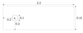
Figure 1: Shown above is the domain for the flow past a cylinder test problem.

There is no external forcing for this test, no-slip boundary conditions are enforced on the walls and cylinder, and an inflow/outflow profile

$$u_{1}(0,y,t) =u_{1}(2.2,y,t)=\frac{6}{0.41^{2}}y(0.41-y),$$

$$u_{2}(0,y,t) =u_{2}(2.2,y,t)=0$$

is enforced as a Dirichlet boundary condition. Of interest for comparisons and accuracy testing are the predicted lift and drag, and for these quantities we use the definitions

$$c_{d}(t) =20\int_{S}\left(\nu\frac{\partial u_{t_{S}}(t)}{\partial n}n_{y}-p(t)n_{x}\right)dS,$$

$$c_{l}(t) =20\int_{S}\left(\nu\frac{\partial u_{t_{S}}(t)}{\partial n}n_{x}-p(t)n_{y}\right)dS,$$

where $u_{t_{S}}$ is the tangential velocity, $S$ the cylinder, and $n=\langle n_{x},n_{y}\rangle$ is the outward unit normal vector. For the calculations, we used the global integral formulation from [15].

4.2 Full order model simulations

To study the performance of the LRTD–ROM with respect to the spatial mesh refinement, we consider three regular triangulations $\mathcal{T}_{h}$ of $\Omega$. The finest triangulation consists of 62,805 triangles, while the inter-medium and the coarsest meshes have 30,078 and 8,658 triangles; the coarsest mesh is illustrated in Figure 2. We note the triangulations are constructed by first creating a Delaunay triangulation followed by a barycenter refinement (Alfeld split). All FOM simulations used the scheme (3) with time step $\Delta t=0.002$, and lowest order Scott-Vogelius elements as described in section 2. With this choice of elements, the three meshes provided 252,306, 121,064 and 35,020 total spatial degrees of freedom(dof). For a given viscosity $\nu$, the corresponding Stokes solution was found with this element choice and mesh to generate the initial condition.

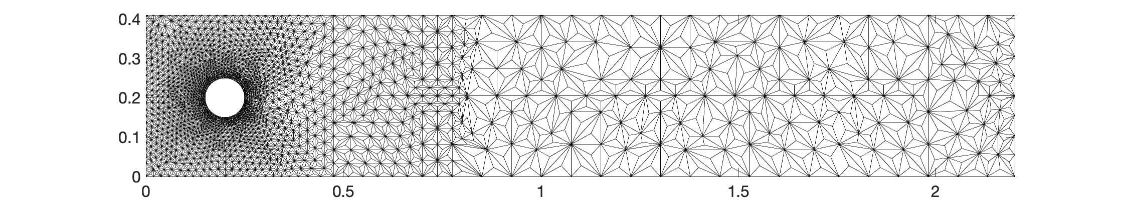
Figure 2: Shown above is the coarsest mesh used for the flow past a cylinder test simulations.

The viscosity parameter sampling set consists of $K$ viscosity values log-uniformly distributed over the interval [$2.5\cdot 10^{-4},4\cdot 10^{-3}$], which corresponds to $25\leq Re\leq 400$. $K=25$ was the maximum value we used for training the ROM, and results are shown below for varying $K$.

All FOM simulations were run for $t\in[0,6]$, and by $t=5$ the von Karman vortex street was fully develop behind the cylinder for $Re\gtrapprox 50$. For $Re<50$, the flows had reached a steady state by $t=5$. For each $\nu$ from the sampling set, 251 velocity snapshots were collected for $t\in[5,6]$ in uniformly distributed time instances. This resulted in a $M\times K\times N$ snapshot tensor $\boldsymbol{\Phi}$, with $M$=dof for each mesh, $K$ different viscosities, and $N=251$. We note that the Stokes extension of the boundary conditions (which is very close to the snapshot average but preserves an energy balance [21]) was subtracted from each snapshot used to build $\boldsymbol{\Phi}$.

4.3 ROM basis and construction

Table 2 shows the dependence of the tensor $\widetilde{\boldsymbol{\Phi}}$ ranks on the targeted compression accuracy $\varepsilon$ and the FOM spatial resolution. The first rank determines the universal space dimension. As expected, higher ranks are needed for better accuracy. At the same time the dependence on spatial resolution is marginal.

	Mesh 1	Mesh 2	Mesh 3
target accuracy / M	35020	121064	252306
$\varepsilon=10^{-1}$	[15,12 ,7]	[15,11,7]	[18,13,8]
$\varepsilon=10^{-2}$	[74,21,40]	[78,21,40]	[89,21,45]
$\varepsilon=10^{-3}$	[190 ,22 ,80]	[213,22,85]	[239,22,93]
$\varepsilon=10^{-4}$	[365,23,113]	[404,23,124]	[444,23,135]

Table 2: HOSVD ranks of the $\varepsilon$-truncated LRTD for the snapshot tensor.

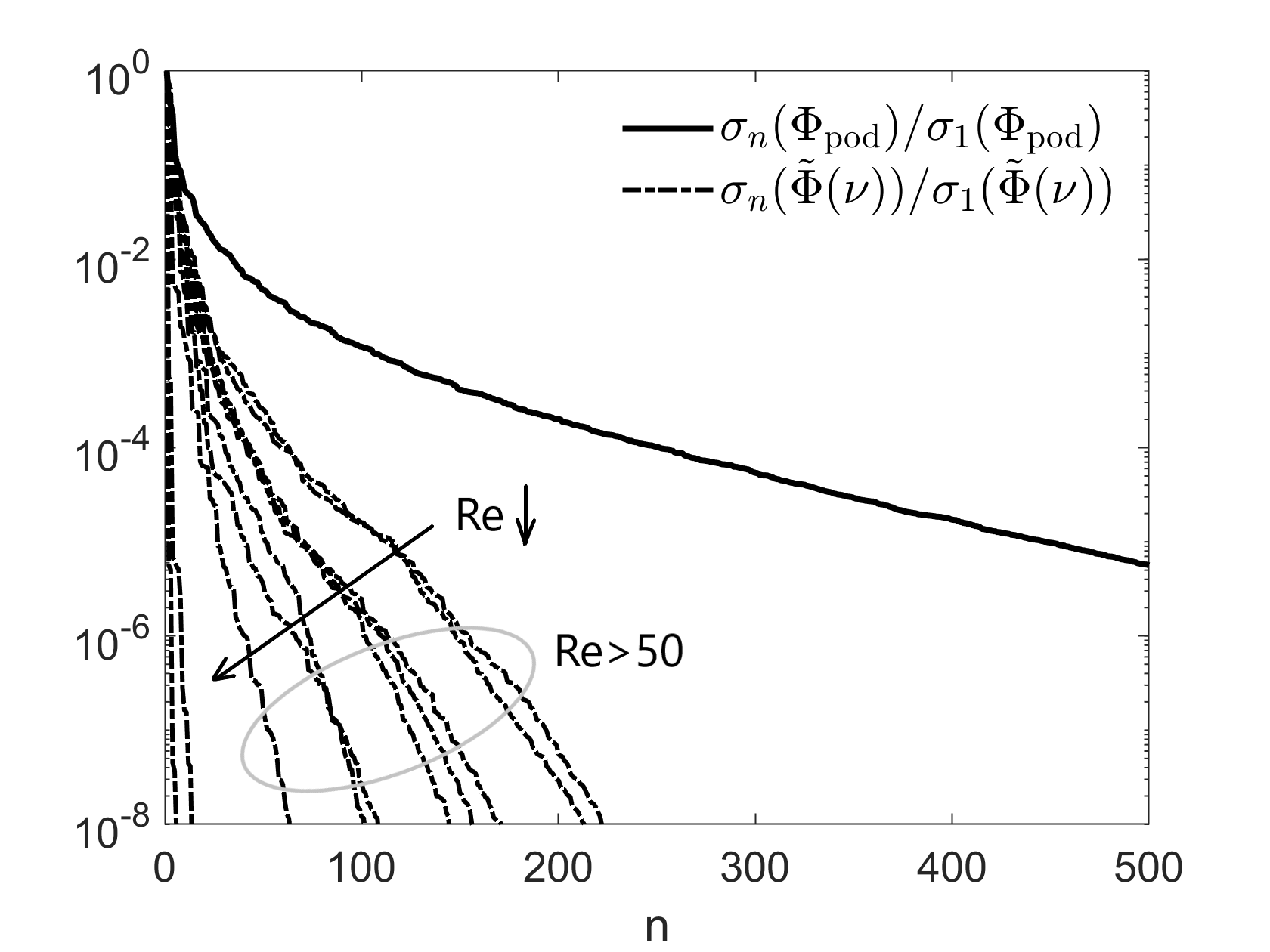
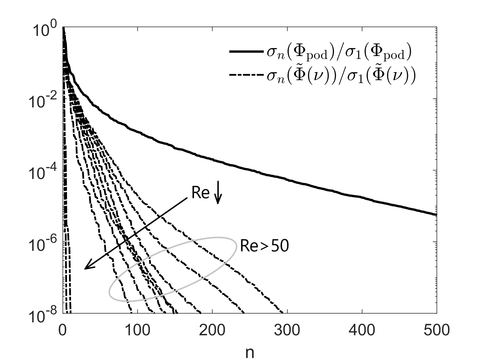
Figure 3: Singular values decay for POD matrix and local LRTD matrix for 10 parameter values. Left and right panels show result for interpolatory and non-interpolatory LRTD–ROMs, respectively.

Figure 3 illustrates on why finding $\nu$-dependent local ROM spaces through LRTD is beneficial compared to employing a POD space, which is universal for all parameter values. The faster decay of singular values $\sigma(\tilde{\Phi}(\nu))$ allows for attainment of the desired accuracy using lower ROM dimensions compared to the POD–ROM. At the same time, the decay rate of $\sigma(\tilde{\Phi}(\nu))$ depends on $\nu$ with faster decay observed for larger viscosity values, i.e. smaller Reynolds numbers. Unsurprisingly, the snapshots collected for $\text{Re}<50$ show very little variability, indicated by the abrupt decrease of $\sigma_{n}$ for $n>1$, since the flow approaches an equilibrium state in these cases.

A plot of the first 7 modes for non-interpolatory LRTD–ROM using $\epsilon=10^{-4}$ with $Re=$110 and 380, and for the full POD constructed with data from tests using all the parameter values, are shown in figure 4. We observe that for the LRTD–ROM cases, the modes quickly go from larger scales in the first few modes to much finer scales by mode 7, whereas for the full POD, the first 7 mode are all still at larger scales. This is consistent with figure 3, which shows the decay of singular values is much slower, meaning more modes are needed to characterize the space.

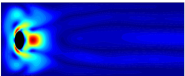
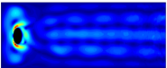
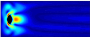
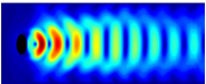
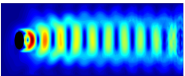
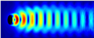
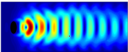
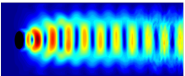
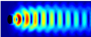
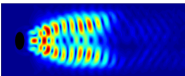
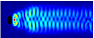
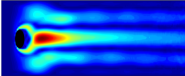
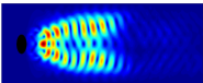
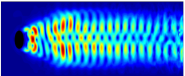
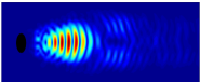
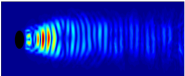
Figure 4: Modes 2,3,4,5,6,7 (from top to bottom) for (left) Re=110 POD-ROM, (center) Re=380 POD-ROM, and (right) universal basis

4.4 ROM accuracy

Table 3: Relative $L^{2}$ norms of the errors between FOM and ROM solutions for 3 values of $Re$ numbers that are not in the training set. The results are for $\ell=20$.

	Re=30		Re=110		Re=380
K	13	25	13	25	13	25
interp. LRTD–ROM	4.1e-7	2.1e-8	1.7e-3	1.7e-3	1.9e-2	1.6e-2
non-interp. LRTD–ROM	1.6e-6	2.2e-7	2.8e-3	2.2e-3	1.8e-2	1.5e-2
POD–ROM	7.6e-5	5.5e-5	5.6e-2	5.2e-2	1.6e-1	9.0e-2

We next study the dependence of the LRTD–ROMs’ solution accuracy on the parameter sampling and the ROM design. We consider two training sets with $K=13$ and $K=25$ viscosity parameters log-uniformly sampled in the parameter domain, i.e. $\nu_{i}=\nu_{\min}\big{(}\frac{\nu_{\max}}{\nu_{\min}}\big{)}^{(i-1)/K}$ for $i=1,\dots,K$. Other parameters of the ROMs were $\varepsilon=10^{-4}$ and $\ell=20$ (dimension of the ROM space). We run ROM simulations for $Re=100$, which corresponds to $\nu=10^{-3}$ from the training sets, and for $Re\in\{30,\,110,\,380\}$, which are viscosity parameters not in the training sets. For the initial flow velocity we use linear interpolation between known velocity values at the two closest points from the training set at $t=5$.

Table 3 shows the relative $L^{2}((5,6)\times\Omega)$ error in three different norms for both interpolatory and non-interpolatory versions of the LRTD–ROM (for both $K=13$ and $K=25$) and compares both to the POD–ROM. We observe that the POD–ROM is worse in all cases, often by an order of magnitude or more. The interpolatory LRTD–ROM is somewhat more accurate in this measure than the non-interpolatory one for $Re=110$ and $Re=30$ but has similar accuracy at $Re=380$.

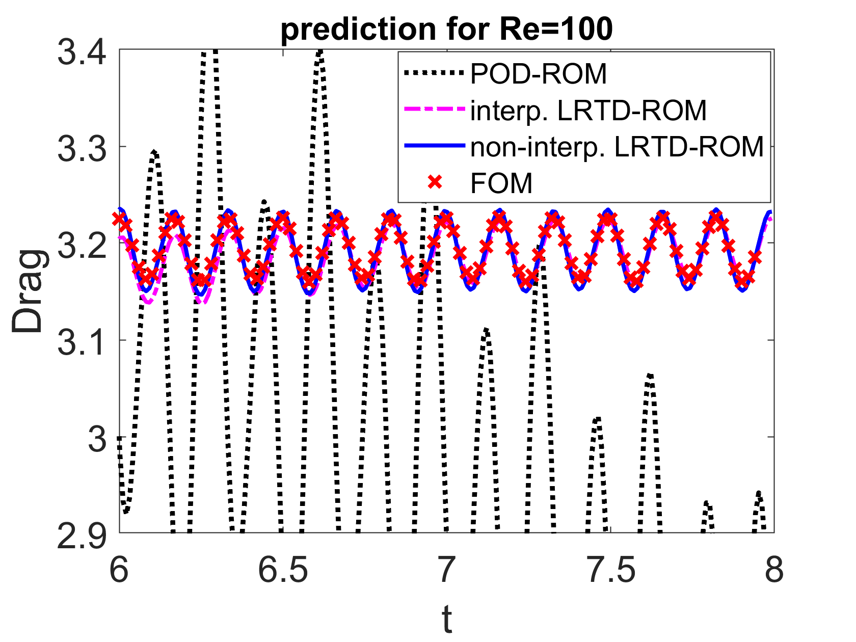
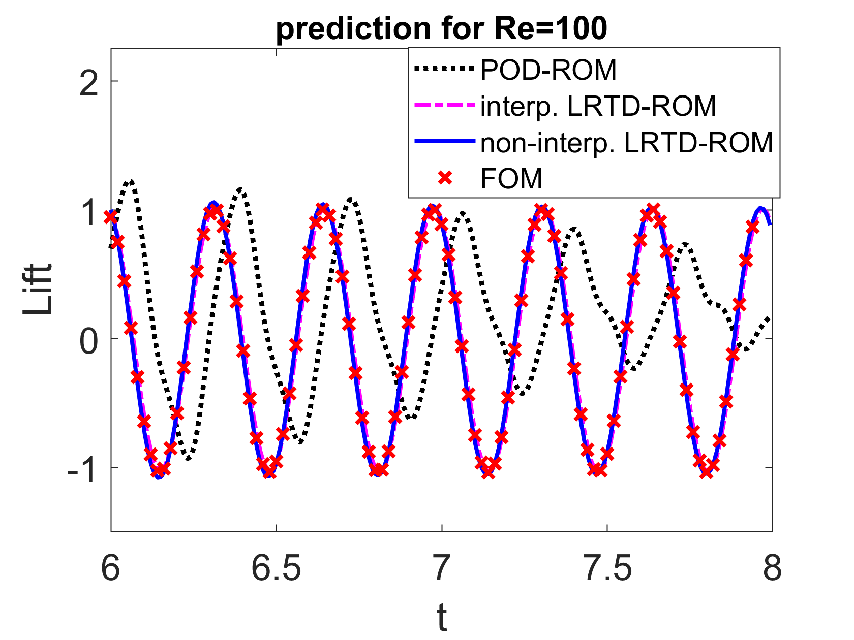
Figure 5: Prediction of lift and drag coefficients for Re=100 (which is in the training set). Number of parameters in the training set is $K=13$, and $\ell=20$.

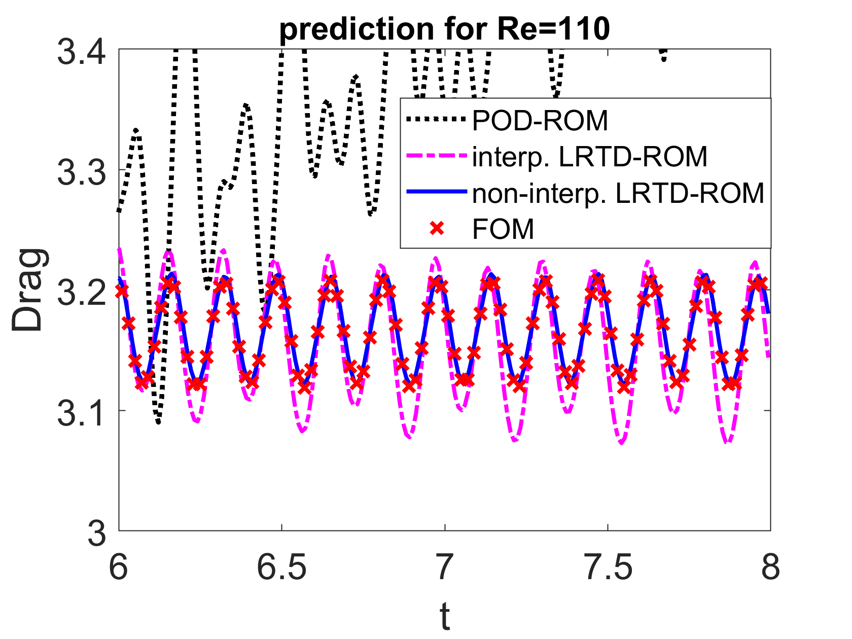
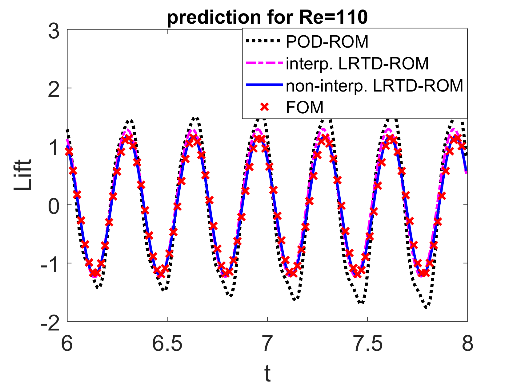
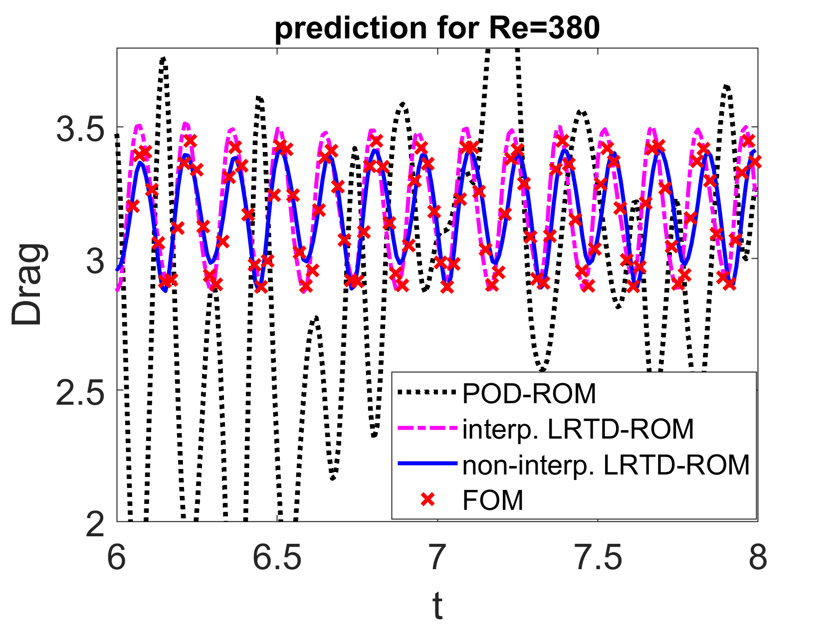
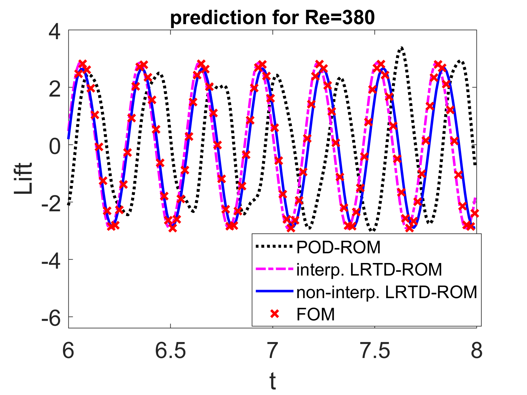
Figure 6: Prediction of lift and drag coefficients for Re=110 and Re=380 not from the training set. Number of parameters in the training set is $K=13$, and $\ell=20$.

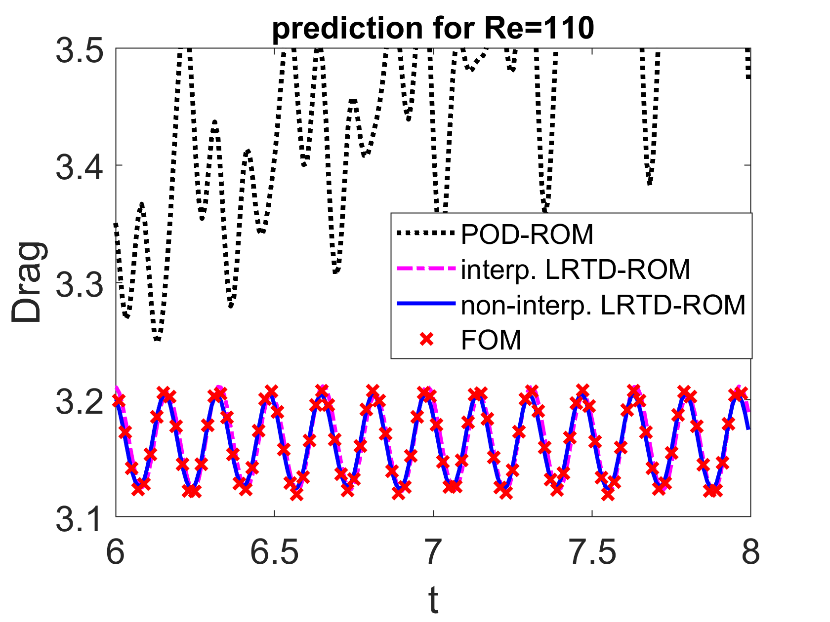
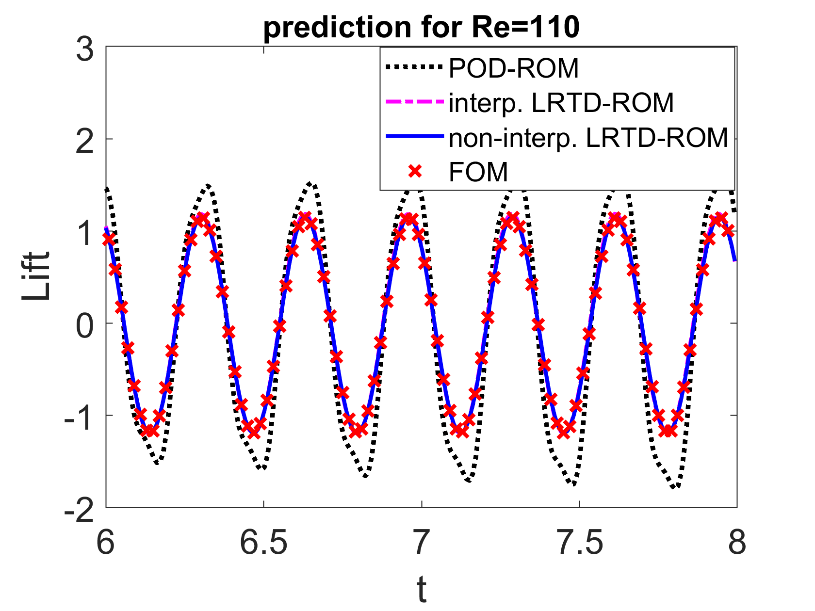
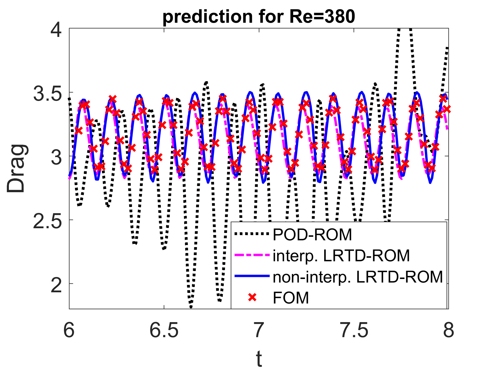
Figure 7: Prediction of lift and drag coefficients for Re=110 and Re=380 not from the training set. Number of parameters in the training set is $K=25$, and $\ell=20$.

In addition to accuracy in norms, we are interested in the ability of the tensor ROMs to predict critical statistics such as drag and lift coefficients for the cylinder. We are interested in the prediction accuracy of the method both outside the training set and beyond the time interval used to collect the snapshots. The results for $Re=100$ and $K=13$ are shown in Figure 5. We note that $Re=100$ is in the training set, and observe that the interpolatory and non-interpolatory LRTD-ROM results were quite good, and match the FOM flow lift and drag quite well. The POD-ROM results, however, were very inaccurate. As discussed above, the POD-ROM may need many more modes to be able to capture finer scale detail that the LRTD-ROMs are able to capture.

The results for $Re=110$ and $Re=380$ are presented in Figure 6 for $13$ parameters in the training set and in Figure 7 for $25$ parameters in the training set. The plots are for $6\leq t\leq 8$, since we are not starting with the “correct” flow state and the system may take some time to reach the quasi-equilibrium (periodic) state. We observe that for both $K=13$ and $K=25$, POD-ROM results are inaccurate. For $K=25$, both interpolatory and non-interpolatory results are reasonably accurate, although for $Re=380$ the drag predictions show some slight error. For $K=13$, results are less accurate; in the latter case, we observe non-interpolatory LRTD-ROM results to be slightly better compared to interpolatory LRTD-ROM (similar accuracy is found for total kinetic energy plots, which are omitted).

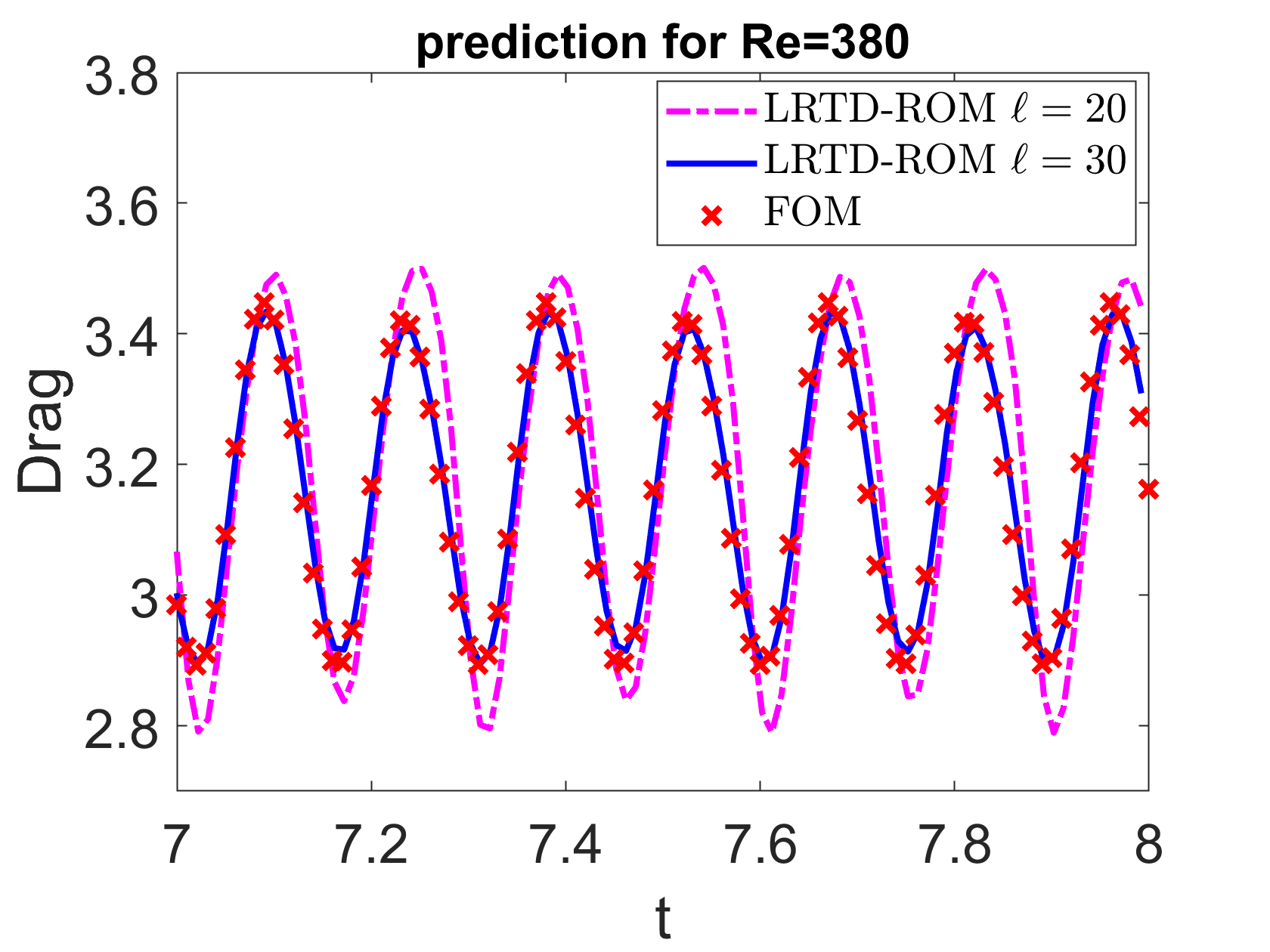
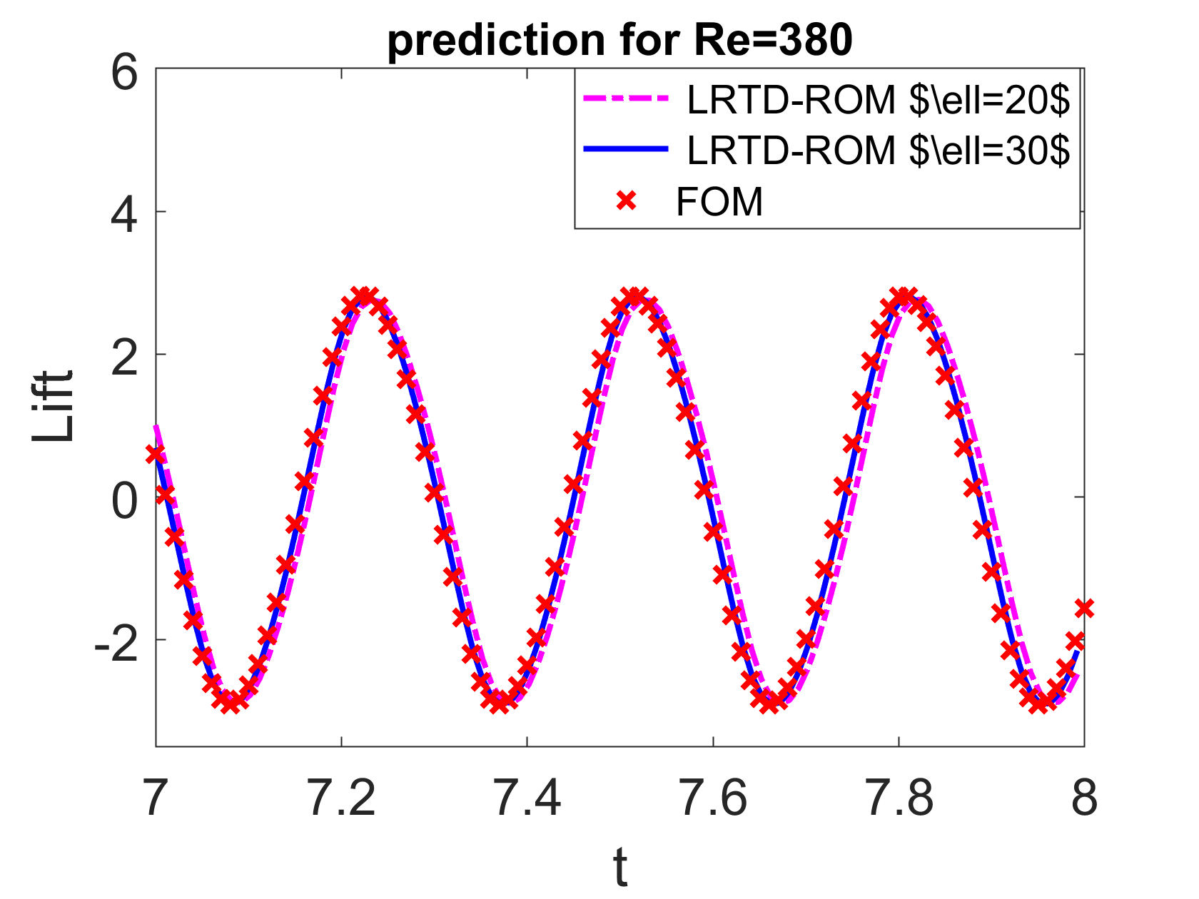
Figure 8: Prediction of drag and lift coefficients for $Re=380$ with non-interpolatory LRTD–ROM dimensions $\ell=20$ and $\ell=30$. Number of parameters in the training set is $K=25$.

Increasing the dimension of the LRTD–ROM improves the accuracy, as should be expected. The effect is illustrated in figure 8, which shows the results for the non-interpolatory LRTD–ROM with $\ell=20$ and $\ell=30$. While the results for the lift prediction are almost indistinguishable, for the drag coefficient $\ell=30$ has the ROM and FOM values match, while $\ell=20$ is seen to slightly overshoot minimal and maximal values for $Re=380$. Thus for further simulations we chose the non-interpolatory LRTD–ROM with $\ell=30$, and trained on the set of $25$ parameters.

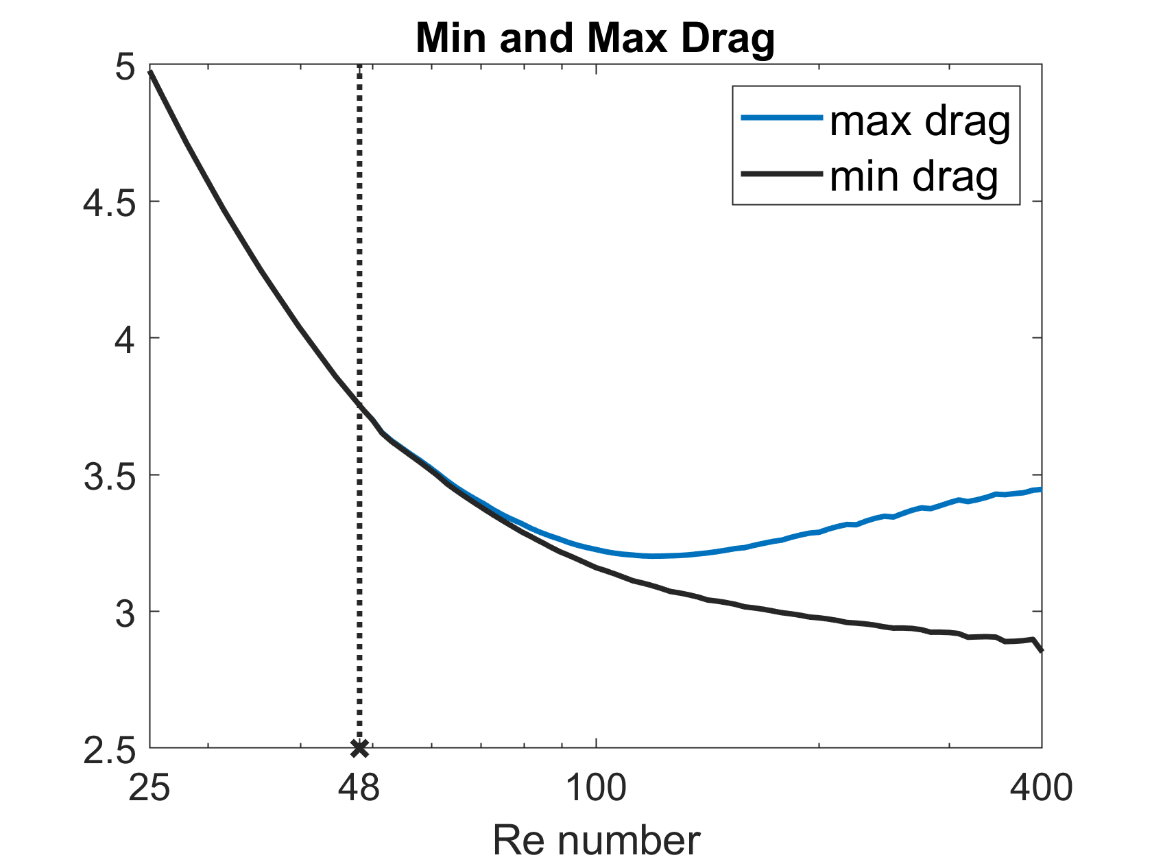
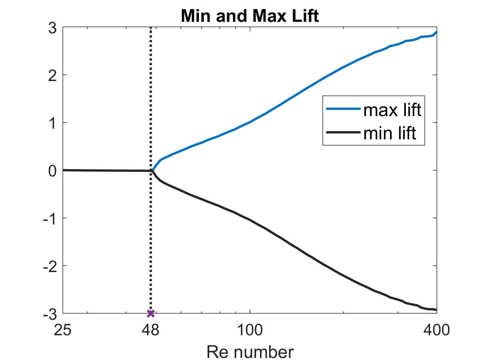
Figure 9: Minimal and the maximal values of drag and lift coefficients along the smooth branch of solutions.

4.5 Predicting an entire branch of solutions

We are interested in applying the ROM to approximate the flow statistics along the whole branch of solutions, and for these tests we use non-interpolatory LRTD–ROM with $\ell=30$ and $K=25$. To this end, we run the LRTD-ROM for 99 viscosity values log-uniformly sampled in our parameter domain and calculate the solution up to final $T=50$ starting from an initial condition which is interpolated from snapshots at $t_{0}=5$. Figure 9 shows the predicted lift and drag coefficient’s variation for varying $Re$, after quasi-periodic state is reached in each flow. We find the transition point from steady-state to periodic flow to be near $Re=48$, which agrees closely with the literature [4, 27].

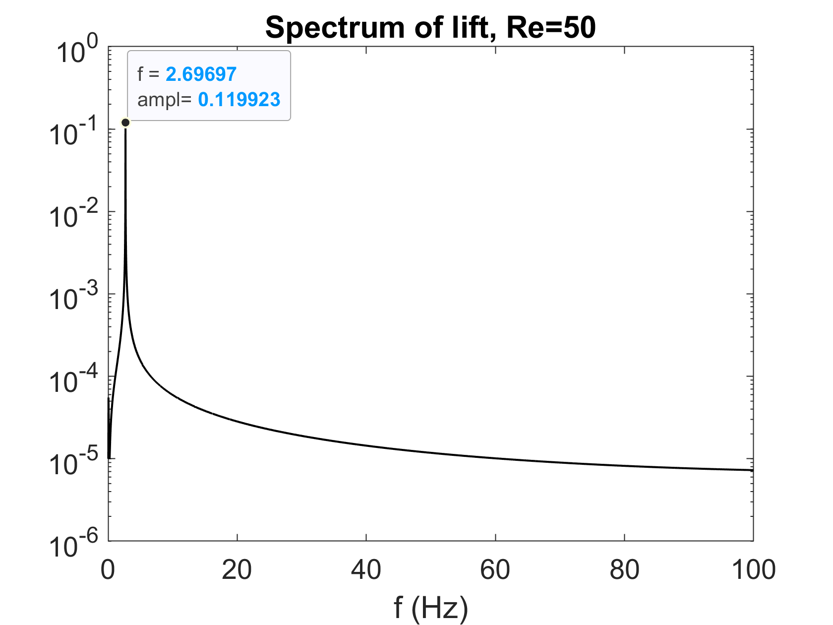
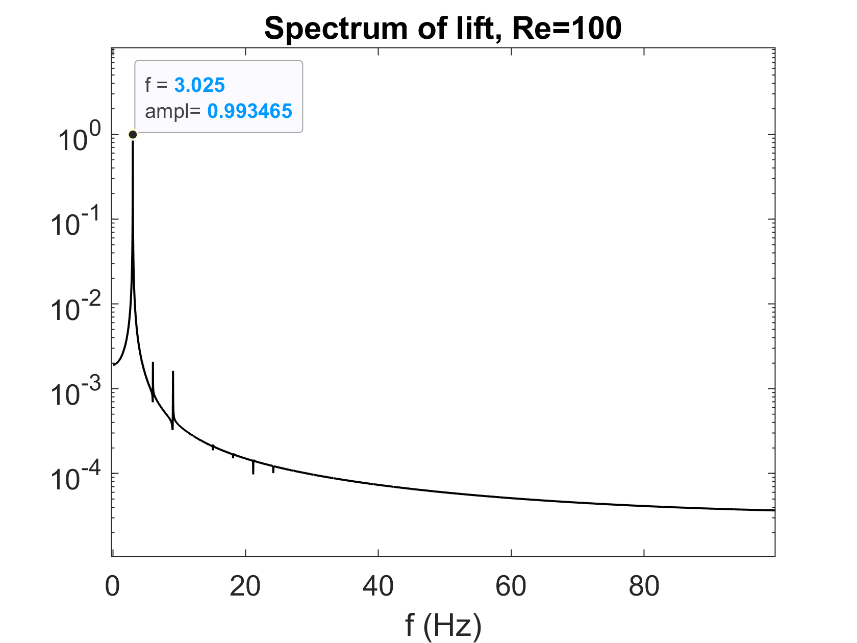
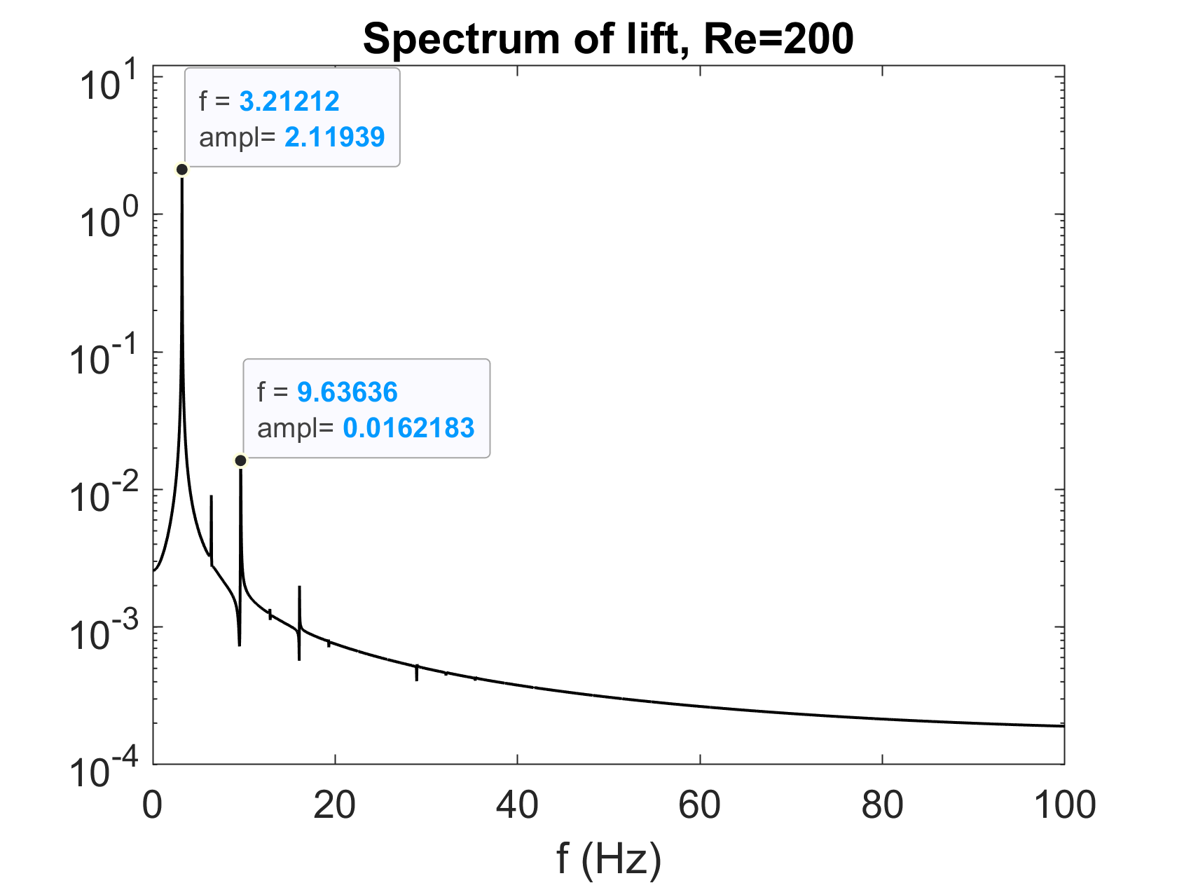
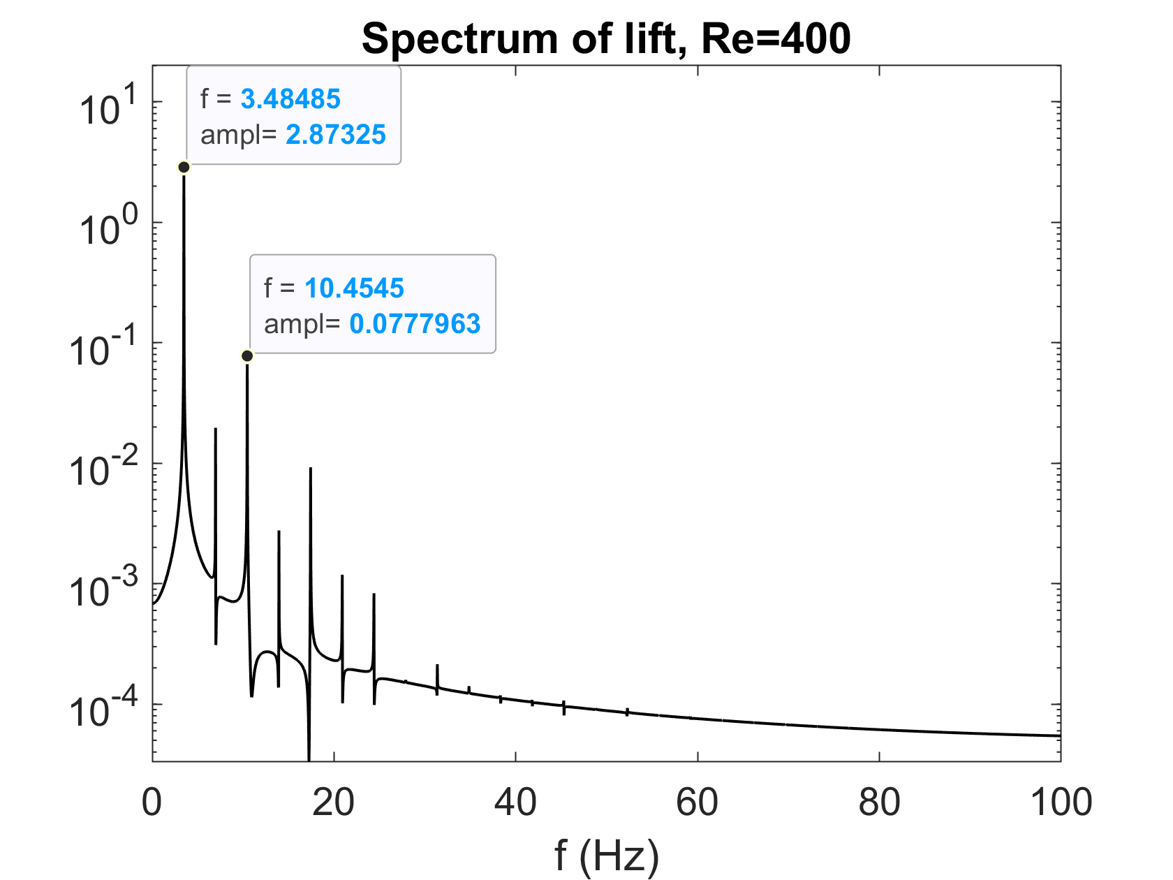
Figure 10: Shown below are spectrums of the lift coefficients for varying $Re$.

We next consider the spectrum of the flow statistics by computing the Fourier transform of the lift coefficient for time interval $t\in[10,50]$. In Figure 10, this is shown for $Re$=50, 100, 200 and 400. For $Re=50$, only one spike is observed, indicating a single dominant frequency. For $Re=100$, some smaller spikes are shown in the plot, but they are nearly 3 orders of magnitude smaller than the largest spike and have minimal effect on the solution’s periodicity. By $Re=200$, the second biggest spike is a little over two orders of magnitude smaller than the biggest one, and by $Re=400$ there is less than two orders of magnitude difference suggesting that this flow is moving away from a purely periodic flow to one with more complex behavior in time.

Besides building more effective ROM, the LRTD may offer new insights into the properties of parametric solutions. To give an example, let us consider the HOSVD singular vectors of $\boldsymbol{\Phi}$. Figure 11 shows several dominant vectors in time and parameter directions, which are the first several HOSVD singular vectors of the snapshot tensor in the time and parameter modes. Larger amplitudes of parameter singular vectors with Re number increase suggest higher sensitivity of flow patterns to the variation of the viscosity parameter, for flows with larger Reynolds numbers.

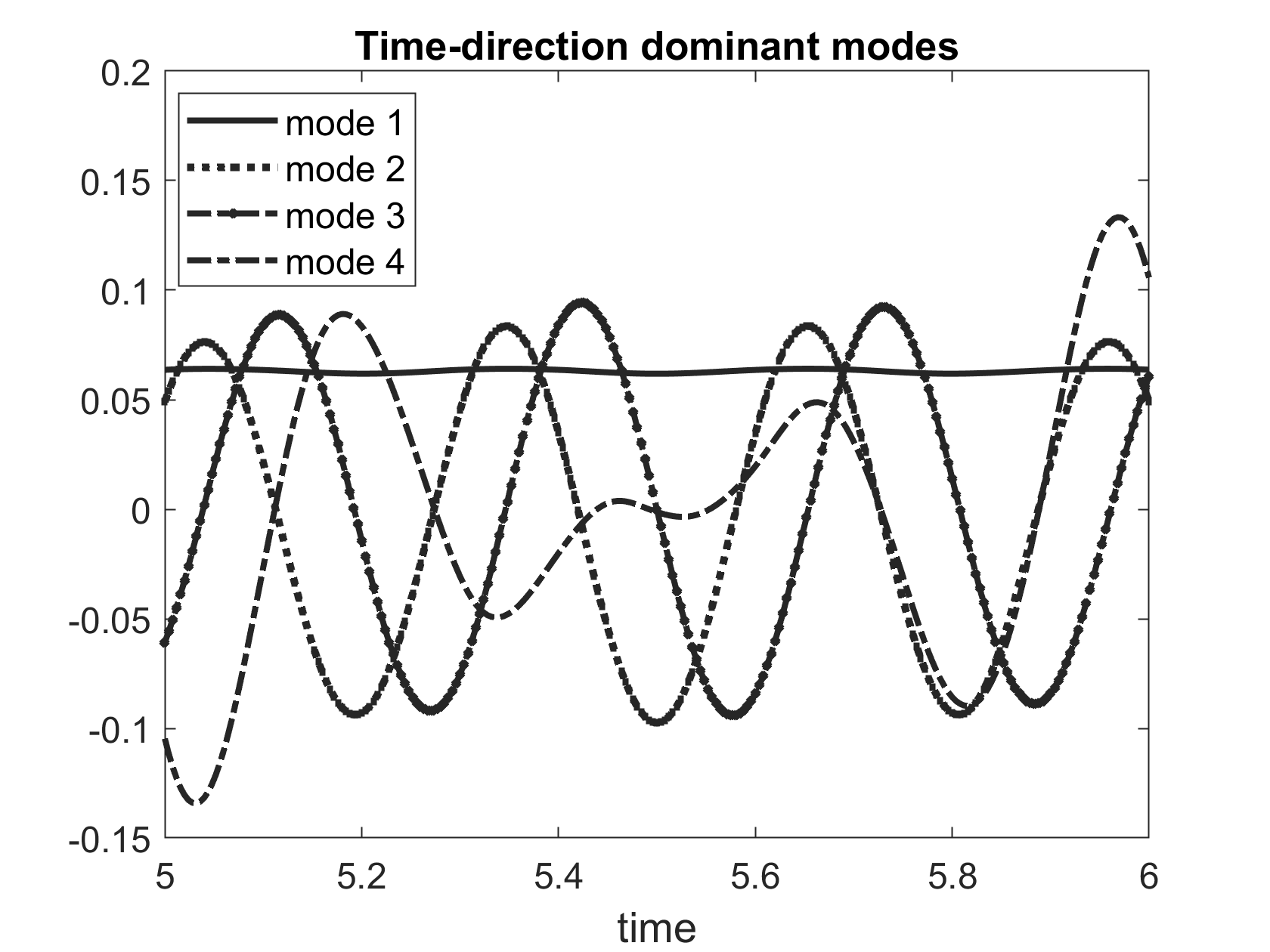
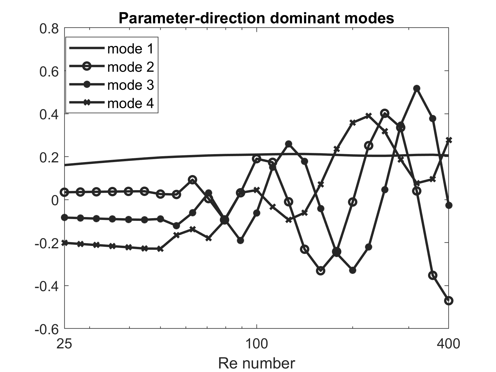
Figure 11: First four HOSVD singular vectors in time and parameter modes.

The first singular vectors in time and space direction are approximately constant, cf. Fig. 11.

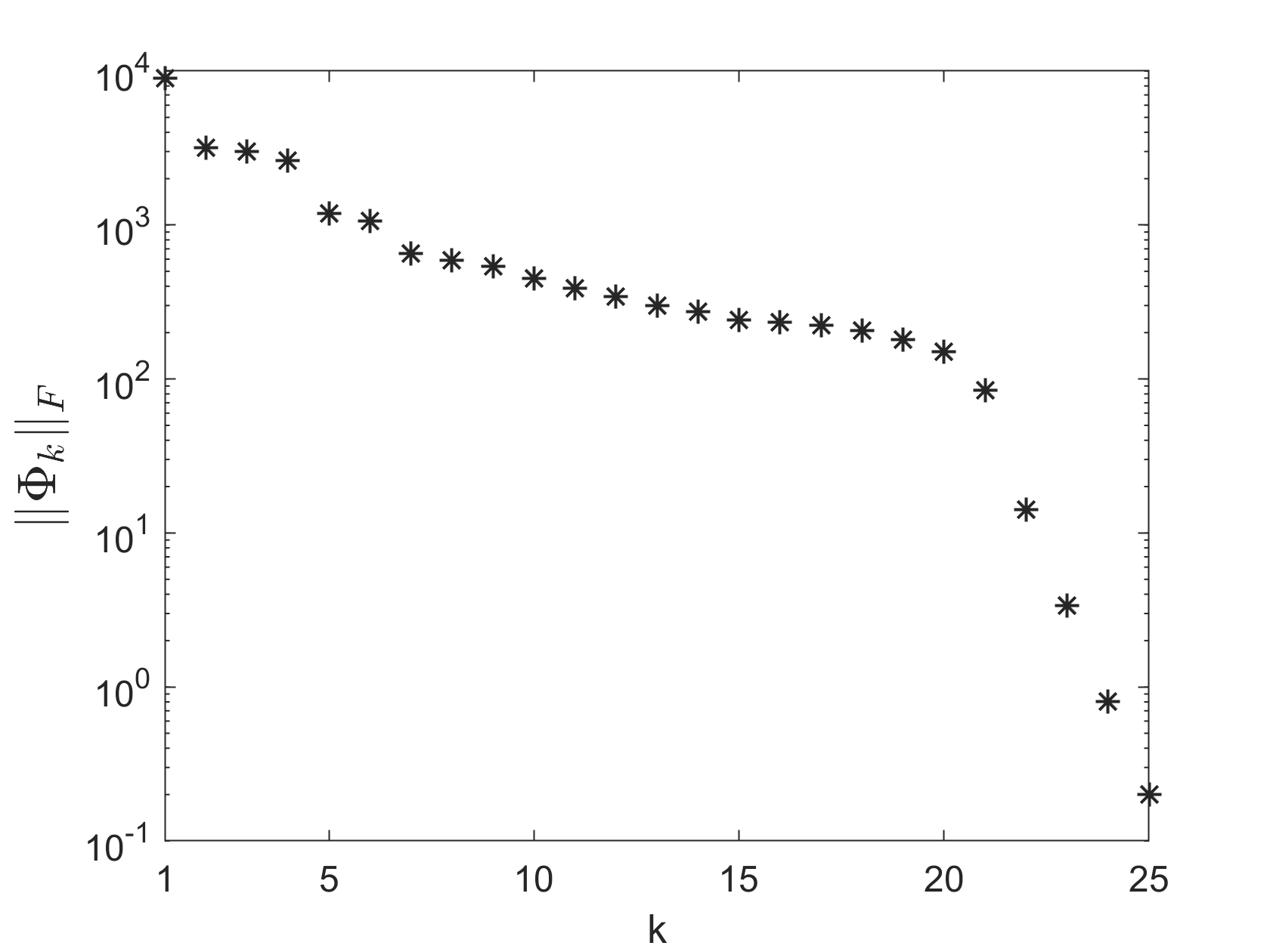
Figure 12: Frobenius norms of space-time stuctures $\Phi_{k}$ from decomposition (20).

This indicates that the parametric solution possesses dominant space–parameter and space–time states which are persistent in time and Reynolds number, respectively. Let us focus on persistence in Reynolds number. For HOSVD, the $\boldsymbol{\sigma}$ vectors from (9) are the first $\widetilde{K}$ singular vectors of the second mode unfolding of $\boldsymbol{\Phi}$, and so $\boldsymbol{\Phi}$ can be written as the sum of $K$ direct products:

(20) $$\boldsymbol{\Phi}=\sum_{k=1}^{K}\Phi_{k}\otimes\boldsymbol{\sigma}^{k},$$

where $\Phi_{k}\in\mathbb{R}^{M\times N}$ are space–time states (note that these are not actual physical states) whose evolution in Reynolds number is determined by $\boldsymbol{\sigma}^{k}$. Matrices $\Phi_{k}$ are mutually orthogonal in the sense of the element-wise product, $\mbox{tr}(\Phi_{k}\Phi_{j}^{T})=0$ for $k\neq j$, and since $\|\Phi_{k}\|_{F}$ equals the $k$-th singular value of the second mode unfolding of $\boldsymbol{\Phi}$, it also holds that

$$\|\Phi_{1}\|_{F}\geq\|\Phi_{2}\|_{F}\geq\dots\geq\|\Phi_{K}\|_{F}.$$

Figure 12 shows the norms of the persistent space–time states. We see that $\Phi_{1}$ is not overly dominating and about 20 persistent space–time states contribute to the parametric solution. Using orthogonality of $\boldsymbol{\sigma}^{k}$ one finds from (20) that

(21) $$\Phi_{k}=\boldsymbol{\Phi}\times_{2}\boldsymbol{\sigma}^{k}.$$

Therefore, $\Phi_{k}$ are easily recovered for $k=1,\dots,\widetilde{K}$ once $\boldsymbol{\sigma}^{k}$ are provided by HOSVD LRTD. From (21) and the observation that $\boldsymbol{\sigma}^{1}$ is nearly constant in Re, we conclude that the dominant space–time state $\Phi_{1}$ is close to a scaled average of the parametric solution in Reynolds number (similar conclusion holds for the dominant space–parameter state — it is close to a scaled time averaged solution).

To gain further insight into the structure of $\Phi_{1}$, we display in Figure 13 the dominant spatial modes of $\Phi_{1}$. These are obtained by computing the SVD of $\Phi_{1}$. Singular values of $\Phi_{1}$ drop rapidly so that the first spatial mode, shown in Figure 13, captures nearly 99.9% of the energy.

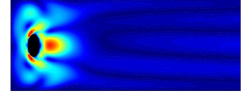
1. 2.
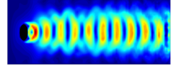
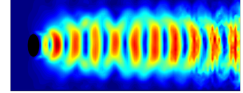
3. 4.

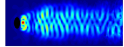
Figure 13: Shown above are the first four spatial modes, taken from $\Phi_{1}$, the first space-time persistent state.

5 Conclusions

The LRTD-ROM, an extension of a POD-ROM for parametric problems, retains essential information about model variation in the parameter domain in a reduced order format. When applied to the incompressible Navier-Stokes equations parameterized with the viscosity coefficient, the LRTD-ROM facilitates accurate prediction of flow statistics along a smooth branch of solutions. Moreover, it enables the identification of parameter structures that may not be apparent through standard POD analysis.

Previously, LRTD-ROMs have demonstrated success in addressing multi-parameter linear and scalar non-linear problems. A natural next step is to extend it to multi-parameter problems of fluid dynamics. Additionally, current research efforts are directed towards developing LRTD-ROMs based on sparse sampling of the parametric domain.

References

- [1] F. Andreuzzi, N. Demo, and G. Rozza, A dynamic mode decomposition extension for the forecasting of parametric dynamical systems, SIAM Journal on Applied Dynamical Systems, 22 (2023), pp. 2432–2458.
- [2] D. N. Arnold and J. Qin, Quadratic velocity/linear pressure Stokes elements, Advances in Computer Methods for Partial Differential Equations, 7 (1992), pp. 28–34.
- [3] A. Caiazzo, T. Iliescu, V. John, and S. Schyschlowa, A numerical investigation of velocity–pressure reduced order models for incompressible flows, Journal of Computational Physics, 259 (2014), pp. 598–616.
- [4] J.-H. Chen, W. Pritchard, and S. Tavener, Bifurcation for flow past a cylinder between parallel planes, Journal of Fluid Mechanics, 284 (1995), pp. 23–41.
- [5] P. Constantin and C. Foias, Global Lyapunov exponents, Kaplan–Yorke formulas and the dimension of the attractors for 2D Navier–Stokes equations, Communications on Pure and Applied Mathematics, 38 (1985), pp. 1–27.
- [6] L. De Lathauwer, B. De Moor, and J. Vandewalle, A multilinear singular value decomposition, SIAM Journal on Matrix Analysis and Applications, 21 (2000), pp. 1253–1278.
- [7] A. Ern and J.-L. Guermond, Theory and practice of finite elements, vol. 159, Springer, 2004.
- [8] Z. Gao, Y. Lin, X. Sun, and X. Zeng, A reduced order method for nonlinear parameterized partial differential equations using dynamic mode decomposition coupled with k-nearest-neighbors regression, Journal of Computational Physics, 452 (2022), p. 110907.
- [9] V. Girault and P.-A. Raviart, Finite element methods for Navier–Stokes equations: theory and algorithms, vol. 5, Springer Science & Business Media, 2012.
- [10] M. Guo and J. S. Hesthaven, Data-driven reduced order modeling for time-dependent problems, Computer Methods in Applied Mechanics and Engineering, 345 (2019), pp. 75–99.
- [11] W. Hackbusch, Tensor spaces and numerical tensor calculus, vol. 42, Springer, 2012.
- [12] W. Hackbusch and S. Kühn, A new scheme for the tensor representation, Journal of Fourier analysis and applications, 15 (2009), pp. 706–722.
- [13] M. W. Hess, A. Quaini, and G. Rozza, A data-driven surrogate modeling approach for time-dependent incompressible Navier–Stokes equations with dynamic mode decomposition and manifold interpolation, Advances in Computational Mathematics, 49 (2023), p. 22.
- [14] J. G. Heywood and R. Rannacher, Finite-element approximation of the nonstationary Navier–Stokes problem. part iv: error analysis for second-order time discretization, SIAM Journal on Numerical Analysis, 27 (1990), pp. 353–384.
- [15] V. John, Reference values for drag and lift of a two dimensional time-dependent flow around a cylinder, International Journal for Numerical Methods in Fluids, 44 (2004), pp. 777–788.
- [16] E. N. Karatzas, M. Nonino, F. Ballarin, and G. Rozza, A reduced order cut finite element method for geometrically parametrized steady and unsteady Navier–Stokes problems, Computers & Mathematics with Applications, 116 (2022), pp. 140–160.
- [17] T. G. Kolda and B. W. Bader, Tensor decompositions and applications, SIAM Review, 51 (2009), pp. 455–500.
- [18] A. V. Mamonov and M. A. Olshanskii, Interpolatory tensorial reduced order models for parametric dynamical systems, Computer Methods in Applied Mechanics and Engineering, 397 (2022), p. 115122.
- [19] A. V. Mamonov and M. A. Olshanskii, Analysis of a tensor POD–ROM for parameter dependent parabolic problems, arXiv preprint arXiv:2311.07883, (2023).
- [20] A. V. Mamonov and M. A. Olshanskii, Tensorial parametric model order reduction of nonlinear dynamical systems, arXiv preprint arXiv:2302.08490 (to appear in SIAM Journal on Scientific Computing), (2023).
- [21] M. Mohebujjaman, L. Rebholz, X. Xie, and T. Iliescu, Energy balance and mass conservation in reduced order models of fluid flows, Journal of Computational Physics, 346 (2017), pp. 262–277.
- [22] F. Pichi, F. Ballarin, G. Rozza, and J. S. Hesthaven, An artificial neural network approach to bifurcating phenomena in computational fluid dynamics, Computers & Fluids, 254 (2023), p. 105813.
- [23] R. Reyes, O. Ruz, C. Bayona-Roa, E. Castillo, and A. Tello, Reduced order modeling for parametrized generalized Newtonian fluid flows, Journal of Computational Physics, 484 (2023), p. 112086.
- [24] M. Schfer and S. Turek, The benchmark problem ‘flow around a cylinder’ flow simulation with high performance computers II, in E.H. Hirschel (Ed.), Notes on Numerical Fluid Mechanics, 52, Braunschweig, Vieweg (1996), pp. 547–566.
- [25] G. Stabile and G. Rozza, Finite volume POD-Galerkin stabilised reduced order methods for the parametrised incompressible Navier–Stokes equations, Computers & Fluids, 173 (2018), pp. 273–284.
- [26] L. R. Tucker, Some mathematical notes on three-mode factor analysis, Psychometrika, 31 (1966), pp. 279–311.
- [27] C. H. Williamson, Vortex dynamics in the cylinder wake, Annual Review of Fluid Mechanics, 28 (1996), pp. 477–539.