Two Toy Spin Chain Models of Decoherence

Abstract

We solve for the decoherence dynamics of two models in which a simple qubit or ‘Central Spin’ couples to a bath of spins; the bath is made from a chain of spins. In model 1, the bath spins are Ising spins; in Model 2, they are coupled by transverse spin-spin interactions, and the chain supports spin waves. We look at (i) the case where the Hamiltonian is static, with a constant system/bath coupling, and (ii) where this coupling varies in time.

I Introduction

The dynamics of ‘decoherence’, ie., the gradual entanglement of a quantum system with its environment - is of considerable subtlety. In the simplest picture, one imagines some sort of exponential decay in time of off-diagonal matrix elements in a reduced density matrix for the central system. For a single central spin or ‘qubit’, this would occur on a timescale $T_{2}$, distinct from the time $T_{1}$ for the decay of the diagonal matrix elements.

This simple picture is only correct under very restrictive conditions - it is correct, eg., for a central spin coupled to random noise. Solutions for the dynamics of the ‘spin-boson’ model [1, 2] (where the central qubit couples to an oscillator bath) or the ‘central spin’ model [3] (where the central spin couples to a bath of spins) show much more complicated behaviour. In the central spin model, one can see quite complex non-monotonic behaviour in time of the density matrix elements. If one then looks at the correlations between the central system and the environmental variables, extremely complex features emerge, in which entanglement correlators at different levels exchange information in interesting ways [4, 5].

Even more complex features can emerge when the central system goes beyond a simple two-level ‘qubit’ system, to some object hopping on some lattice. This is a topic of considerable interest to those interested in the decoherence dynamics of quantum information processing systems (a huge topic), in the dynamics of quantum walks [7, 8, 9], in the well known problem of motion of holes in insulating magnetic systems [9, 10, 11, 12, 13], and anyone interested in general problems in quantum diffusion.

Quite generally the models that are employed fall into 2 classes, viz.,

(i) Oscillator Bath Models: In such models the environment is modelled as a set of independent oscillators [2]; these are supposed to represent extended modes (like phonons, photons, electron-hole pairs, gravitons, etc.). For a system containing $N$ such oscillators, the coupling of the system to each oscillator is $\propto N^{-1/2}$, so that for large $N$ (or for $N\rightarrow\infty$) the effect of the bath on the central system is independent of $N$, and one can assume an equilibrium bath at some temperature $T$.

(ii) Spin Bath Models: The environment is now modelled as a set of ‘pseudospin’ degrees of freedom [3], each possessing a finite-dimensional Hilbert space (often a 2-dimensional space, so that the environment is a set of 2-level systems). These represent localized modes (like defects, nuclear or paramagnetic spins, or dynamic impurities in the system). In this case the coupling between the central system and each bath ‘spin’ may not depend on $N$ at all, and certainly there is no requirement that it be $\propto N^{-1/2}$. One cannot assume that this bath is in equilibrium.

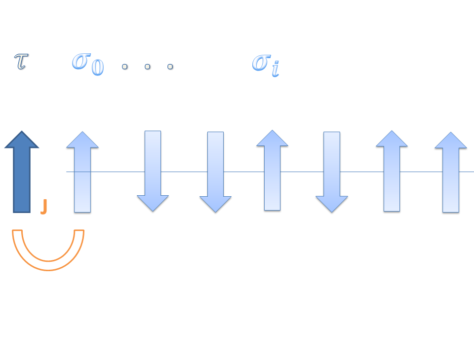
Figure 1: Illustration of our spin chain model. A central spin couples to a spin chain.

For an elementary discussion of the difference between these two baths, see, eg., ref. [14, 15]. A key difference is that for oscillator baths, decoherence is closely tied to dissipation: one expects a fluctuation/dissipation connection to exist. However for spin baths, no such necessary connection exists - in fact, one can have very large decoherence with almost no dissipation. This makes spin baths much more dangerous for, eg., quantum computation.

In this paper we wish to show some very basic features of decoherence dynamics, by choosing two simple ‘toy’ models. The models are of some pedagogical interest, just because they are so simple - indeed, they are sufficiently simple that in one case we easily find an exact solution, and in the other case a very accurate solution in the regime of interest. In this short contribution we first introduce the models, and give the details of their solutions, and then make some observations based on these solutions. It will be seen that even in these simple models (about as simple as one can get) there are several interesting features, which persist in more complicated models.

It will be clear that much more can be said, which we have no space for in this short communication. We will also have no space to discuss the application of models of decoherence that are similar to the ones discussed here. For recent discussions of both anomalous diffusion and localization, which can occur when the decoherence is non-Markovian, work on optical lattices is of some interest [16, 17, 18, 19]; models rather close in spirit to the models discussed here are examined in ref. [8, 9, 20]. More general work on entanglement and decoherence in condensed matter systems is reviewed by LaFlorencie [6].

In both models, the environment is modelled as a 1-D spin chain $\{\sigma_{i}\}$, and the central system is a single spin $\tau$, which is coupled to the first spin in the chain. The models differ only in the form of the bath Hamiltonian.

II Model 1

The first model has an environment or bath with ‘Ising’ Hamiltonian, coupled transversely to a qubit, via a single coupling $J$ between the qubit and the first spin on the spin chain. The Hamiltonian is:

$$H=J\tau^{y}\sigma_{0}^{y}+V\sum_{i=0}^{N-1}\sigma_{i}^{z}\sigma_{i+1}^{z},$$ (1)

where $\tau^{y}$ is the central spin operator and the $\{\sigma_{i}\}$ are operators for $N$ bath spins; $J$ is the coupling between the central qubit and the first bath spin, and $NV$ is the band width of the bath spins. We do not use periodic boundary conditions here.

The central spin has the reduced density matrix

$$\begin{pmatrix}|a|^{2}&a^{*}b\kappa(t)\\ ab^{*}\kappa^{*}(t)&|b|^{2}\end{pmatrix}.$$ (2)

This model can be solved exactly. Since $H$ commutes with $\tau^{y}$, the diagonal component (represented in $\tau^{y}$ eigenstates) of the reduced density matrix does not change in time. We write the off-diagonal components $\rho_{12}(t)$ and $\rho_{21}(t)$ as

$$\rho_{12}(t)=\kappa(t)\rho_{12}(0),$$ (3)

with $\kappa(t)$ being the “decoherence factor”

$$\kappa=\mbox{tr}_{b}\left(e^{-iH^{+}t}\rho_{b}e^{-iH^{-}t}\right),$$ (4)

where $H^{\pm}$ are the block Hamiltonians in the $\tau^{y}=\pm 1$ subspaces respectively:

$$H^{\pm}\;=\;\pm J\sigma_{0}^{y}+V\sum_{i=0}^{N-1}\sigma_{i}^{z}\sigma_{i+1}^{z}$$ (5)

The solution to this model is

$$\kappa(t) = \frac{V^{2}+J^{2}\cos 2\sqrt{1+J^{2}/V^{2}}t}{V^{2}+J^{2}}$$ (6)

$$= 1-\frac{2J^{2}\sin^{2}\sqrt{1+J^{2}/V^{2}}t}{V^{2}+J^{2}}.$$

which is clear enough - one is basically dealing with a 2-spin problem, because there is no coupling between the spins on the chain. Thus all correlations and information existing initialy in the qubit are confined to the qubit/bath spin pair.

It is also interesting to obtain an approximate solution to this problem. To do this we use a Jordan-Wigner transformation to diagonalize $H$, by writing

$$\sigma_{i}^{z} = -\prod_{j<i}(1-2c_{j}^{{\dagger}}c_{j})(c_{i}^{{\dagger}}+c_{i}),$$ (7)

$$\sigma_{i}^{x} = 1-2c_{i}^{{\dagger}}c_{i},$$ (8)

$$\sigma_{i}^{y} = i\prod_{j<i}(1-2c_{j}^{{\dagger}}c_{j})(c_{i}^{{\dagger}}-c_{i}).$$ (9)

Substituting this into (1) gives

$$H = iJ\tau^{y}(c_{0}^{{\dagger}}-c_{0})$$ (10)

$$\qquad+V\sum_{i=0}^{N-1}(c_{i}^{{\dagger}}c_{i+1}^{{\dagger}}-c_{i}c_{i+1}^{{\dagger}}+c_{i}^{{\dagger}}c_{i+1}-c_{i}c_{i+1}).$$

Introducing the Fourier transform $c_{k_{n}}=\frac{1}{\sqrt{N}}\sum_{j}c_{j}e^{ijk_{n}}$, with $k_{n}=\frac{2\pi n}{N}$, and the Bogoliubov transformation

$$\gamma_{k_{n}} = e^{-\frac{ik_{n}}{2}}\left(\cos\frac{k_{n}}{2}c_{k_{n}}-i\sin\frac{k_{n}}{2}c_{-k_{n}}^{{\dagger}}\right),$$ (11)

$$c_{k_{n}} = \cos\frac{k_{n}}{2}e^{\frac{ik_{n}}{2}}\gamma_{k_{n}}+i\sin\frac{k_{n}}{2}e^{\frac{ik_{n}}{2}}\gamma_{-k_{n}}^{{\dagger}}.$$ (12)

the Hamiltonian becomes

$$\begin{split}H&=\sum_{n}\left(V(2\gamma_{k_{n}}^{{\dagger}}\gamma_{k_{n}}-1)+\frac{iJ}{\sqrt{N}}\tau^{y}(\gamma_{k_{n}}^{{\dagger}}-\gamma_{k_{n}})\right)\\ &=\sum_{n}H_{n},\end{split}$$ (13)

with $H_{n}=V(2\gamma_{k_{n}}^{{\dagger}}\gamma_{k_{n}}-1)+\frac{iJ}{\sqrt{N}}\tau^{y}(\gamma_{k_{n}}^{{\dagger}}-\gamma_{k_{n}})$.

Now the individual Hamiltonians $H_{n}$ do not commute with each other; we have

$$[H_{n},H_{n^{\prime}}]=-\frac{2J^{2}}{N}(\gamma_{k_{n}}^{{\dagger}}-\gamma_{k_{n}})(\gamma_{k_{n^{\prime}}}^{{\dagger}}-\gamma_{k_{n^{\prime}}}).$$ (14)

However, in the weak interaction limit $J/\sqrt{N}V\ll 1$, these commutators can be neglected (see Appendix), and the Hamiltonian (13) becomes block diagonal. In each $\{\gamma_{k_{n}}^{{\dagger}},\gamma_{k_{n}}\}$ subspace, we have

$$H_{n}(\tau^{y}=+1) = \begin{pmatrix}1&\frac{iJ}{\sqrt{N}V}\\ -\frac{iJ}{\sqrt{N}V}&-1\end{pmatrix}$$ (15)

$$H_{n}(\tau^{y}=-1) = \begin{pmatrix}1&-\frac{iJ}{\sqrt{N}V}\\ \frac{iJ}{\sqrt{N}V}&-1\end{pmatrix}.$$ (16)

Let’s assume the bath is initially in a fully mixed state $\rho_{B}=\frac{1}{2}\mathbf{I}$. It is then straightforward to calculate $\kappa(t)$:

$$\begin{split}\kappa&=1-2\sin^{2}(\sqrt{1+\frac{J^{2}}{NV^{2}}}t)\frac{J^{2}}{NV^{2}+J^{2}}\\ &\approx 1-2\sin^{2}t\frac{J^{2}}{NV^{2}}.\end{split}$$ (17)

so that as $N\to\infty$, we have:

$$\kappa=\lim_{N\to\infty}\left(1-2\sin^{2}t\frac{J^{2}}{NV^{2}}\right)^{N}=e^{-2J^{2}\sin^{2}t/V^{2}}.$$ (18)

which gives the correct result up to order $J^{2}/V^{2}$.

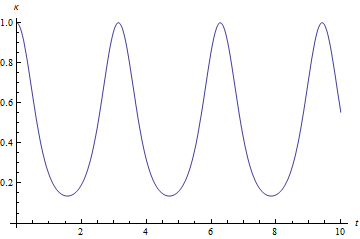
Figure 2: Decoherence factor $\kappa(t)$ (18) of model 1 as a function of time. There is no real decoherence and $\kappa$ goes back to 1 periodically.

We see that $\kappa$ is periodic in time (see Fig. 2). This is because, as already noted, information cannot flow into the whole spin chain - it is confined to the first local bath spin and the central spin.

III Model 2

We now consider another model in which the spin chain is the environment, but in which there are interactions between the bath spins (here, simple transverse spin-spin coupling). The model Hamiltonian is

$$H=J\tau^{y}\sigma_{0}^{y}+V\sum_{i=0}^{N-1}(\sigma_{i}^{+}\sigma_{i+1}^{-}+h.c.).$$ (19)

in which spin waves can propagate down the chain. Thus the environment is now a set of oscillators (spin waves); this model is a variant of the spin-boson model.

Again using the Jordan-Wigner transformation, we have

$$H=\sum_{n}\left(2V\cos k_{n}(\gamma_{k_{n}}^{{\dagger}}\gamma_{k_{n}}-\frac{1}{2})-\frac{iJ}{\sqrt{N}}\tau^{y}(\gamma_{k_{n}}^{{\dagger}}-\gamma_{k_{n}})\right).$$ (20)

which has the same structure as (13), except now with bath spectrum $\cos k_{n}V$ instead of a constant. We now follow the same approximate procedure used for model 1, to get the decoherence factor up to order $J^{2}$:

$$\begin{split}\frac{1}{2}\mbox{tr}\left(e^{-iH_{n}^{-}t}e^{-iH_{n}^{{\dagger}}t}\right)&=1-\frac{2\sin^{2}\sqrt{V^{2}\cos^{2}k_{n}+\frac{J^{2}}{N}}t}{\cos^{2}k_{n}+\frac{J^{2}}{NV^{2}}}\cdot\frac{J^{2}}{NV^{2}}\\ &\approx 1-\frac{2\sin^{2}(Vt\cos k_{n})J^{2}}{NV^{2}\cos^{2}k_{n}};\quad\quad(N\to\infty)\\ &\approx e^{-\frac{2\sin^{2}(Vt\cos k_{n})J^{2}}{NV^{2}\cos^{2}k_{n}}}.\end{split}$$ (21)

After including all the $H_{n}$s, we finally get

$$\kappa(t)=\exp\left(-\sum_{n}\frac{2\sin^{2}(Vt\cos k_{n})J^{2}}{NV^{2}\cos^{2}k_{n}}\right)$$ (22)

If we now take the limit $N\rightarrow\infty$, this reduces to

$$\begin{split}\kappa(t)&\approx\exp\left(-\frac{J^{2}}{\pi V^{2}}\int^{\pi}_{-\pi}dk\frac{\sin^{2}(Vt\cos k)}{\cos^{2}k}\right);\quad\quad(N\to\infty)\\ &=\exp\left(-2J^{2}t^{2}\,_{1}F_{2}\left(\frac{1}{2};\frac{3}{2},2;-V^{2}t^{2}\right)\right).\end{split}$$ (23)

where ${}_{1}F_{2}$ is a hypergeometric function.

The resulting behaviour of $\kappa(t)$ is illustrated in Fig. 3. Its long time asymptotic behaviour can still be studied. When $t\to\infty$, we can expand the generalized hypergeometric function as

$$(Vt)^{2}\,_{1}F_{2}\left(\frac{1}{2};\frac{3}{2},2;-V^{2}t^{2}\right)\;\;=\;\;Vt\;+\;\frac{1}{2}\sqrt{\frac{1}{\pi Vt}}\cos\left(2Vt-\frac{\pi}{4}\right)+O\left(\frac{1}{(Vt)^{\frac{3}{2}}}\right).$$ (24)

and we see that $\kappa\to e^{-J^{2}t/V}\to 0$ as $t\to\infty$.

We see that in this model the system decoheres completely as $t\rightarrow\infty$; the quantum information is forever lost to the environment, into the spin wave bath. In fact, we are dealing here with a particular species of spin-boson model.

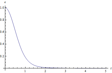
Figure 3: This is the decoherence factor of model 2 as a function of time. The loss of coherence is clear over time.

IV Time-Varying System-Bath Coupling

What if we are allowed to switch on or off the coupling between the central system and the bath? One can envisage several such situations - for example, we can simply switch the coupling off, or we can switch it off and then bring it back again, in an effort to reverse the decoherence.

IV.1 Switch-off process

Let us assume a time-varying coupling $J(t)$ of form:

$$H=J(t)\tau^{y}\sigma_{0}^{y}+H_{bath},$$ (25)

where $J(t)\to J_{0}$ as $t\to-\infty$ and $J(t)\to 0$ as $t\to\infty$. We choose a convenient model form for $J(t)$ to be

$$J(t)=\frac{J_{0}}{e^{kt}+1}.$$ (26)

so that $\frac{d}{dt}J(t)=-J_{0}ke^{kt}/(e^{kt}+1)^{2}$.

Figure 4: Figure of the coupling $J(t)$ over time. These lines represent $k=0.1,0.5,1,10$ respectively.

We see that when $k\to 0$, $\frac{d}{dt}J(t)$ will go to zero; when $k\to\infty$, it will become a Heaviside step function with a jump at $t=0$ (see Fig.4 ). These 2 limits describe two complementary processes. The $k=0$ limit simply adiabatically decouple the system from the bath, whereas the $k\rightarrow\infty$ limit suddenly switches off the coupling. For this sudden decoupling case, the result should be the same as what we get from previous sections since the central system stops evolving after the turn-off. But for the adiabatic decoupling case, things are more complicated - we need to solve the problem explicitly - we will do this in the long-time limit.

IV.2 Time-dependent solutions

With the time-dependent $J(t)$ we can follow the same Jordan-Wigner/Bogoliubov procedure as before, and now transform the Hamiltonian to

$$H=\sum_{n}2E_{n}(\gamma_{n}^{{\dagger}}\gamma_{n}-\frac{1}{2})+\sum\frac{iJ(t)}{\sqrt{N}}(\gamma_{n}^{{\dagger}}-\gamma_{n}),$$ (27)

where $E_{n}=V$ for model 1, and $E_{n}=V\cos k_{n}$ for model 2. Then we have

$$H_{n}^{\pm}=\begin{pmatrix}2E_{n}&\mp\frac{iJ(t)}{\sqrt{N}}\\ \pm\frac{iJ(t)}{\sqrt{N}}&0\end{pmatrix}.$$ (28)

Our goal is to solve this Hamiltonian in each $\{\gamma_{n}^{{\dagger}}|0\rangle,|0\rangle\}$ subspace. A vector $(a(t),b(t))$ in this subspace evolves as

$$-i\begin{pmatrix}\frac{d}{dt}a(t)\\ \frac{d}{dt}b(t)\end{pmatrix}=\begin{pmatrix}2E_{n}&\mp\frac{iJ(t)}{\sqrt{N}}\\ \pm\frac{iJ(t)}{\sqrt{N}}&0\end{pmatrix}\begin{pmatrix}a(t)\\ b(t)\end{pmatrix}.$$ (29)

so that

$$a(t)=\mp\frac{\sqrt{N}}{J(t)}\dot{b}(t),$$ (30)

$$\ddot{b(t)}-(iE_{n}+\frac{\dot{J}(t)}{J(t)})\dot{b}(t)+\frac{J^{2}(t)}{N}b(t)=0.$$ (31)

After some derivation (see Appendix), we get a result for $\kappa(t)$ from this. The long time asymptotic limit $t\rightarrow\infty$ of $\kappa(t)$ is then:

$$\kappa(t)=\prod_{n}(1-\frac{2J^{2}}{NE_{n}^{2}}).$$ (32)

For the two models we then have:

(i) Model 1: Here we have $H_{bath}=V\sum_{i=0}^{N-1}\sigma_{i}^{z}\sigma_{i+1}^{z}$, and $E_{n}=V$ for all subspaces. Then the decoherence factor is

$$\kappa_{1}(t)=(1-\frac{2J^{2}}{NE_{n}^{2}})^{N}=e^{-2J_{0}^{2}}.$$ (33)

(ii) Model 2: Now we have $H_{bath}=V\sum_{i=0}^{N-1}(\sigma_{i}^{+}\sigma_{i+1}^{-}+h.c.)$, and $E_{n}=V\cos k_{n}$ for each subspaces. The decoherence factor is

$$\kappa_{2}(t)=e^{-\frac{1}{2\pi}\int_{0}^{2\pi}dk\frac{2J^{2}}{V^{2}\cos^{2}k}}\to 0.$$ (34)

Thus, in this adiabatically decoupled limit, we find “partial decoherence” for model 1 ($\kappa\rightarrow e^{-2J^{2}}$)and “complete decoherence” for model 2 ($\kappa\rightarrow 0$). Apparently, system 1 ends up in a mixed state and the coherence is partially lost.

However, appearances are deceptive in this case. To see this, we can imagine reversing the coupling back to its original value. We therefore consider what happens for a general slow-varying $J(t)$. In this case (31) still holds, and we can consider both models 1 and 2.

(i)Model 1: Here again we have $E_{n}=V$. If the coupling is varying slowly, $\dot{J(t)}\ll J(t)E_{n}$, we can safely neglect the $dJ/dt$ term in (31) and we have

$$\begin{split}b(t)=&C_{1}e^{-iVt/2-iVt/2\sqrt{1+\frac{4J^{2}(t)}{NV^{2}}}}+C_{2}e^{-iVt/2+iVt/2\sqrt{1+\frac{4J^{2}(t)}{NV^{2}}}},\\ a(t)=&-\frac{i2C_{1}\sqrt{N}}{J(t)}(V+V\sqrt{1+\frac{4J^{2}(t)}{NV^{2}}})e^{-iVt/2-iVt/2\sqrt{1+\frac{4J^{2}(t)}{NV^{2}}}}\\ &-\frac{i2C_{2}\sqrt{N}}{J(t)}(V-V\sqrt{1+\frac{4J^{2}(t)}{NV^{2}}})e^{-iVt/2+iVt/2\sqrt{1+\frac{4J^{2}(t)}{NV^{2}}}}.\end{split}$$ (35)

We can see that in this adiabatic limit, the result has no dependence on $dJ/dt$. The decoherence factor $\kappa_{1}(t)$ should therefore be solely dependent on the form of $J(t)$. This means that if one slowly changes the coupling strength back to its original value, $\kappa_{1}(t)$ would go back to its original value regardless of the apparent loss of decoherence we obtained in (33). One can thus recover the full coherence by decoupling the model 1 to its environment and then recoupling it back adiabatically. The coherence is not truly lost into the environment, but simply encoded there in the entanglement between the central spin and the first environmental spin. It can be transferred back to the central spin simply by reversing the interaction.

(ii)Model 2: In model 2 we cannot neglect the $\dot{J}(t)$ term, since $E_{n}=V\cos k_{n}$ can be zero. The slow varying condition $dJ/dt\ll J(t)E_{n}$ breaks down for the modes in the center of the band. Actually it is easy to prove that $\kappa(t)$ must stay at $0$ after adiabatically decoupling from the environment, and that never come back to its initial state even if one reverses the interaction. In this case, the coherence is truly lost through the modes near $k_{n}\approx\frac{\pi}{2},\frac{3\pi}{2}$, once we take the limit $N\rightarrow\infty$.

This result is of course typical of a system coupled to an oscillator bath. One can easily generalize the above considerations to a finite-temperature bath.

V Discussion

It is always helpful, in discussing some general physical phenomenon, to have simple toy models which illustrate basic features of the physics. Decoherence is of course very general - it has been studied intensively in contexts ranging from black hole physics [21] and infrared features of quantum field theory [22], as well as in a huge variety of condensed matter systems. Understanding decoherence is also key to doing quantum computation.

As noted in the introduction, there exist thorough studies of decoherence in several well-known models [1, 2, 3]. Even in a simple central spin model, there are several decoherence mechanisms in play [3]; these mechanisms generalize to more general central systems like particles hopping on rings [23] or moving on hyperlattices [8]. In all these models one finds no connection between decoherence and dissipation, quite unlike the case for oscillator bath models like the spin-boson model [1, 2].

The two models here, taken in conjunction with results for the central spin model [3], make it very clear why this is the case. Let us recall the form of the central spin model Hamiltonian: one has

$$H\;=\;H_{CS}+H_{SB},$$ (36)

where the central spin part is

$$H_{CS} = [\Delta_{o}\hat{\tau}_{x}e^{i\sum_{k}(\mbox{\boldmath$\phi$}_{k}+\mbox{\boldmath$\alpha$}_{k}\cdot\mbox{\boldmath$\sigma$}_{k})}+H.c.]$$ (38)

$$\qquad\qquad+(\epsilon_{o}+\sum_{k}\mbox{\boldmath$\lambda$}^{k}\cdot\mbox{\boldmath$\sigma$}_{k})\hat{\tau}_{z}$$

and the spin bath Hamiltonian is

$$H_{SB}\;=\;\sum_{k}{\bf h}_{k}\cdot\mbox{\boldmath$\sigma$}_{k}\;+\;\sum_{k,k^{\prime}}V_{kk^{\prime}}^{\alpha\beta}\sigma_{k}^{\alpha}\sigma_{k^{\prime}}^{\beta}.$$ (39)

in which $\sigma_{k}$ is again the bath spin operator.

Some of the terms in this Hamiltonian are of no special interest here. The Berry phase coupling $\mbox{\boldmath$\phi$}_{k}$ and the topological phase $\mbox{\boldmath$\alpha$}_{k}$ (which leads to topological decoherence [3]) naturally arise in the truncation of the central system to a 2-level system, but are usually quite small in realistic systems.

The ‘orthogonality blocking’ vector coupling $\mbox{\boldmath$\lambda$}^{k}$ is not so easily dismissed - it leads to ‘precessional decoherence’, which is often the major source of decoherence for systems at low $T$. Nevertheless we shall drop it, noting that further work, in which it is included, will be of considerable interest when it comes to applications of these toy models.

Finally, we note that the interaction $V_{kk^{\prime}}^{\alpha\beta}$ between bath spins is often very small (particularly if the spins are nuclear, or if the bath spins are widely separated in space). On longer time scales it does play an essential role (in creating ’fluctuational decoherence’ [3]), but at shorter timescales it can be treated as negligible.

Let us therefore assume that we now drop all these interactions, so that $V_{kk^{\prime}}^{\alpha\beta}=0$, and that $\mbox{\boldmath$\phi$}_{k}=\mbox{\boldmath$\alpha$}_{k}=0$. Then this reduced Central (CS) spin model is simply a generalization of our ‘model 1’, in which the central spin now couples simultaneously to all of the bath spins instead of just the first one in the chain. It is known from the solution to this reduced CS model [3] that decoherence exists in it, provided one averages over the bath spin states. However, if we do not make such an average, then an initially pure state gradually distributes itself over the $N$ spins in the bath [5]. The time evolution will be periodic, just as for ‘model 1’, but now the period is exponentially long (with timescale $\propto\exp N^{1/3}$); after this timescale, the information ‘comes back’ to reconstitute the original central spin state.

Thus model 1 is just the maximum simplification that one can make of the original CS model. Because model 1 is essentially just a 2-spin problem, we get the simple results given above. If we generalize model 1 to allow coupling of the central qubit to some reduced set of $M$ bath spins, then the basic result of the calculation will now be clear - quantum correlations and entanglement will simply be shared over time between the central qubit and the $M$ bath spins, with entanglement between different bath spins mediated by the central spin. Very accurate solutions for a problem of this kind (which is very relevant to experiment) can be found using entanglement correlator methods [4, 5].

Model 2 is not a simplification of any central spin model; instead, as already noted, it is just a special case of the spin-boson model. If we had wanted to, we could have simply derived the form of the Caldeira-Leggett [1] spectral function $J(\omega)$ for this system, and proceeded from there. Note however that if the number $N$ of spins in the chain is finite, we will also get, in model 2, the quantum analogue of Poincar$\acute{e}$ recurrences - but in the calculations given above, we have let $N\rightarrow\infty$. In model 2, the spin wave modes with $k_{n}\approx\frac{\pi}{2},\frac{3\pi}{2}$ serve the purpose of carrying quantum information away from the central spin.

Obviously there is a lot more one can say about these 2 simple models. It will be of interest, for example, to analyse the higher-spin ‘entanglement correlators’ [4, 5] in model 2, and to see what happens as one adds fields $\{{\bf h}_{k}\}$ acting on the bath spins, and/or gradually ‘switches on’ the interaction between the bath spins. Many models are then possible, all of them generalizations of the 2 simple central spin models discussed here.

Finally, we note that one can also generalize these 2 models to deal with a central system in which a particle hops around some site Hamiltonian. This is nothing but a 1-dimensional ‘polaron’ model - with a spin bath background, it is a type of spin polaron system. It is also related to the original model discussed by Feynman for quantum computation [24]. The central system now has a Hamiltonian

$$H_{o}\;=\;-\sum_{<ij>}\left[t_{ij}c_{i}^{\dagger}c_{j}\>e^{iA_{ij}^{0}}+H.c.\right]+\sum_{j}\varepsilon_{j}c_{j}^{\dagger}c_{j}$$ (40)

in which we also admit a Berry phase $A_{ij}^{0}$ connected to hopping between nearest-neighbour sites.

The most general coupling to the spin bath then takes the form

$$V_{int}\;=\; \sum_{k}^{N} [\;\sum_{j}\mbox{\boldmath$F$}_{j}^{k}(\mbox{\boldmath$\sigma$}_{k})\hat{c}_{j}^{\dagger}\hat{c}_{j}$$

$$+ \sum_{ij}(\mbox{\boldmath$G$}_{ij}^{k}(\mbox{\boldmath$\sigma$}_{k})\hat{c}_{i}^{\dagger}\hat{c}_{j}+H.c.)]$$ (41)

with both diagonal coupling $\mbox{\boldmath$F$}_{j}^{k}$ and non-diagonal coupling $\mbox{\boldmath$G$}_{ij}^{k}$ of the hoping particle to the $k$-th bath spin.

We see immediately that if we choose a simple site-diagonal coupling $\mbox{\boldmath$F$}^{k}(\mbox{\boldmath$\sigma$}_{k})$ on each site, making all these couplings the same for each site, and also let the site energy $\varepsilon_{j}$ be the same for each site, then we have another toy model for which concrete calculations can be done. A related model was treated some time ago [23], in which the line was closed to form a ring.

This work was supported by the National Science and Engineering Council of Canada. We thank Tim Cox for discussions.

DEDICATION: This paper is dedicated to my long-time colleague Gordon Semenoff, whom I first met while I was a postdoc, and he already a professor; at that time I was rather awed by him! Since then he has been a welcome source of advice, wisdom, and friendship, with similar views on many things; and we even once wrote a paper [25] together! I wish him many more years happily carving his own path, in the inimitable way he has done up to now.

Appendix A Appendix

Here we derive two key results used in the text, viz., the effect of the non-commutativity of the $\{H_{n}\}$ in the discussion of model 1, and the derivation of the solution used for adiabatic switching for both models.

A.1 Neglecting Commutators

In (14), we noticed that the $H_{n}^{\prime}$s do not commute with each other; in fact

$$[H_{n},H_{n^{\prime}}]=-\frac{2J^{2}}{N}(\gamma_{k_{n}}^{{\dagger}}-\gamma_{k_{n}})(\gamma_{k_{n^{\prime}}}^{{\dagger}}-\gamma_{k_{n^{\prime}}}).$$ (42)

We can use the Zassenhaus formula [26] to get

$$\begin{split}e^{i\sum_{n}H_{n}t}&=\prod_{n}e^{iH_{n}t}\prod_{n_{1}>n_{2}}e^{\frac{t^{2}}{2}[H_{n_{1}},H_{n_{2}}]}\\ &\times\prod_{n_{1}\geq n_{2}\geq n_{3}}e^{\frac{-it^{3}}{6}([H_{n_{1}},[H_{n_{2}},H_{n_{3}}]]+[[H_{n_{1}},H_{n_{2}}],H_{n_{3}}])}....\end{split}$$ (43)

Although the Hamiltonian is not block diagonal in each $\{\gamma_{k_{n}}^{{\dagger}}|0\rangle,|0\rangle\}$ subspace, if we restrict our model to the weak interaction region, i.e. $J\ll 1$, we can omit this commutator since it always comes into the final expression in higher order. For example , for the $\prod_{n_{1},n_{2}}e^{\frac{t^{2}}{2}[H_{n_{1}},H_{n_{2}}]}$ term, we could expand it in powers of $1/N$ and take expectation values

$$\begin{split}&\mbox{tr}_{b}\left(\prod_{n_{1}>n_{2}}e^{\frac{t^{2}}{2}[H_{n_{1}}^{+},H_{n_{2}}^{+}]}\prod_{n_{1},n_{2}}e^{\frac{t^{2}}{2}[H_{n_{1}}^{-},H_{n_{2}}^{-}]}\right)\\ &=\mbox{tr}_{b}\left(e^{-\frac{J^{2}t^{2}}{N}\sum_{n_{1}>n_{2}}(\gamma_{k_{n_{1}}}^{{\dagger}}-\gamma_{k_{n_{1}}})(\gamma_{k_{n_{2}}}^{{\dagger}}-\gamma_{k_{n_{2}}})}\right)\\ &\approx 1-\frac{J^{4}t^{4}}{N^{2}}N(N-1).\end{split}$$ (44)

As we can see in the main text this already happens in the $J^{2}$ order. Therefore in the weakly interacting region, our calculation can be a good approximation to the exact result.

A.2 Adiabatic Decoupling

The goal is to solve the asymptotic solution to the following equation

$$a(t)=\mp\frac{\sqrt{N}}{J(t)}\dot{b}(t)$$ (45)

$$\ddot{b(t)}-(iE_{n}+\frac{\dot{J}(t)}{J(t)})\dot{b}(t)+\frac{J^{2}(t)}{N}b(t)=0.$$ (46)

We first study the evolution of the state $(0,1)$. Actually, the state $(1,0)$ can be treated in the same way just with an opposite sign of $J(t)$ and $E_{n}$. Then we have the initial condition

$$b(t_{0}) = 1$$ (47)

$$\dot{b}(t_{0}) = 0.$$ (48)

Define the following quantity for simplification, keeping in mind that $\frac{J_{0}^{2}}{N}$ is very small

$$\epsilon=\frac{J_{0}^{2}}{N}.$$ (49)

The general solution of the equation (31) is

$$b(t)=C_{1}e^{-iE_{n}t/2-iE_{n}\sqrt{1+4\epsilon/E_{n}^{2}}/2}(1+e^{kt})^{i\sqrt{\epsilon}/k}f_{1}(-e^{kt})\;\;+\;\;C_{2}e^{-iE_{n}t/2+iE_{n}\sqrt{1+4\epsilon/E_{n}^{2}}/2}(1+e^{kt})^{i\sqrt{\epsilon}/k}f_{2}(-e^{kt})$$ (50)

Here we have

$$f_{1}(x) = {}_{2}F_{1}\left(1+\frac{iE_{n}}{2k}+\frac{i\sqrt{\epsilon}}{k}-\frac{iE_{n}}{2k}\sqrt{1+\frac{4\epsilon}{E_{n}^{2}}};\;-\frac{iE_{n}}{2k}+\frac{i\sqrt{\epsilon}}{k}-\frac{iE_{n}}{2k}\sqrt{1+\frac{4\epsilon}{E_{n}^{2}}};\;1-\frac{iE_{n}}{2k}\sqrt{1+\frac{4\epsilon}{E_{n}^{2}}};\;x\right)$$ (51)

$$f_{2}(x) = {}_{2}F_{1}\left(1+\frac{iE_{n}}{2k}+\frac{i\sqrt{\epsilon}}{k}+\frac{iE_{n}}{2k}\sqrt{1+\frac{4\epsilon}{E_{n}^{2}}};\;-\frac{iE_{n}}{2k}+\frac{i\sqrt{\epsilon}}{k}+\frac{iE_{n}}{2k}\sqrt{1+\frac{4\epsilon}{E_{n}^{2}}};\;1+\frac{iE_{n}}{2k}\sqrt{1+\frac{4\epsilon}{E_{n}^{2}}};\;x\right)$$ (52)

We set our initial time $t_{0}\to-\infty$, then $e^{kt}\to 0$ and

$$f_{1,2}(-e^{kt})\to 1.$$ (53)

Therefore

$$\begin{split}b(t_{0})&\;\;=\;\;1\\ &\;\;=\;\;C_{1}e^{-iE_{n}t_{0}/2-iE_{n}t_{0}\sqrt{1+4\epsilon/E_{n}^{2}}/2}\;+\;C_{2}e^{-iE_{n}t_{0}/2+iE_{n}t_{0}\sqrt{1+4\epsilon/E_{n}^{2}}/2};\end{split}$$ (54)

$$\begin{split}\dot{b}(t_{0})\;\;=\;\;&1\\ \;\;=\;\;&C_{1}(-iE_{n}/2-iE_{n}\sqrt{1+4\epsilon/E^{2}}/2)e^{-iE_{n}t_{0}/2-iE_{n}t_{0}\sqrt{1+4\epsilon/E_{n}^{2}}/2}\\ &+C_{2}(-iE_{n}/2+iE_{n}\sqrt{1+4\epsilon/E_{n}^{2}}/2)e^{-iE_{n}t_{0}/2+iE_{n}t_{0}\sqrt{1+4\epsilon/E_{n}^{2}}/2}\end{split}$$ (55)

Then we can get the constant $C_{1},C_{2}$ as

$$C_{1} = \frac{1}{2}e^{iE_{n}t_{0}/2+iE_{n}t_{0}\sqrt{1+4\epsilon/E_{n}^{2}}/2}(-1+(1+\frac{4\epsilon}{E_{n}^{2}})^{-\frac{1}{2}})$$ (56)

$$C_{2} = \frac{1}{2}e^{iE_{n}t_{0}/2-iE_{n}t_{0}\sqrt{1+4\epsilon/E_{n}^{2}}/2}(1+(1+\frac{4\epsilon}{E_{n}^{2}})^{-\frac{1}{2}}).$$ (57)

After we get the solution , we can study its behavior when $t\to\infty$. We use the fact that when $t\to\infty$

$$f_{1}(-e^{kt}) \to Ae^{iE_{n}t/2-i\sqrt{\epsilon}t+\frac{itE_{n}}{2}\sqrt{1+4\epsilon/E_{n}^{2}}/2}$$ (58)

$$f_{2}(-e^{kt}) \to Be^{iE_{n}t/2-i\sqrt{\epsilon}t-\frac{itE_{n}}{2}\sqrt{1+4\epsilon/E_{n}^{2}}/2}$$ (59)

with

$$A = \frac{\Gamma(1-\frac{iE_{n}}{k}\sqrt{1+4\epsilon/E_{n}^{2}})\Gamma(1+\frac{iE_{n}}{k})}{\Gamma(1+\frac{iE_{n}}{2k}-\frac{i\sqrt{\epsilon}}{k}-\frac{iE_{n}}{k}\sqrt{1+4\epsilon/E_{n}^{2}})}\times\frac{1}{\Gamma(1+\frac{iE_{n}}{2k}+\frac{i\sqrt{\epsilon}}{k}-\frac{iE_{n}}{k}\sqrt{1+4\epsilon/E_{n}^{2}})}$$ (60)

$$B = \frac{\Gamma(1+\frac{iE_{n}}{k}\sqrt{1+4\epsilon/E_{n}^{2}})\Gamma(1+\frac{iE_{n}}{k})}{\Gamma(1+\frac{iE_{n}}{2k}-\frac{i\sqrt{\epsilon}}{k}+\frac{iE_{n}}{k}\sqrt{1+4\epsilon/E_{n}^{2}})}\times\frac{1}{\Gamma(1+\frac{iE_{n}}{2k}+\frac{i\sqrt{\epsilon}}{k}+\frac{iE_{n}}{k}\sqrt{1+4\epsilon/E_{n}^{2}})}.$$ (61)

Recalling that $\epsilon=\frac{J_{0}^{2}}{N}$ is a very small number, we can expand the solution according in powers of $\epsilon$. The results are as follows:

Zeroth order

: if $\epsilon=0$, then $C_{1}\to 0$, $C_{2}\to 1$, and

$$B\to\frac{\gamma(1+\frac{iE_{n}}{k})\gamma(1+\frac{iE_{n}}{k})}{\gamma(1+\frac{iE_{n}}{k})\gamma(1+\frac{iE_{n}}{k})}\to 1.$$ (62)

Thus we find that $b(t)\to 1$, which is exactly what we expected.

First order

Since $\sqrt{1+\frac{4\epsilon}{E_{n}^{2}}}\approx 1+\frac{2\epsilon}{E^{2}}$, we have

$$C_{1} \to e^{iE_{n}t_{0}}(1+\frac{i\epsilon t}{E_{n}})(-\frac{\epsilon}{E^{2}})=-\frac{\epsilon}{E_{n}^{2}}e^{iE_{n}t_{0}}$$ (63)

$$C_{2} \to e^{-i\epsilon t_{0}/E_{n}^{2}}(1-\frac{\epsilon}{E_{n}})=1-\frac{\epsilon}{E_{n}^{2}}-\frac{i\epsilon t}{E_{n}^{2}}.$$ (64)

As a result

$$A \;\;\to\;\; \Gamma(1-\frac{iE_{n}}{k})\Gamma(1+\frac{iE_{n}}{k})\times\Bigg{[}1-\frac{i\epsilon}{kE_{n}}\left(\frac{\Gamma^{\prime}(1-iE_{n}/k)}{\Gamma(1-iE_{n}/k)}+i\Gamma^{\prime}(1)\right)\;+\;\frac{\epsilon}{E_{n}^{2}}(\Gamma^{\prime}(1)-\Gamma^{\prime\prime 2}(1))\Big{]}$$

$$B \;\;\to\;\; 1-\frac{\Gamma^{\prime 2}(1+\frac{iE_{n}}{k})}{\Gamma(1+\frac{iE_{n}}{k})^{2}}\frac{\epsilon}{k^{2}}+\frac{\Gamma^{\prime\prime}(1+\frac{iE}{k})}{\Gamma(1+i\frac{E_{n}}{k})}\frac{\epsilon}{k^{2}};$$ (65)

so that for $b(t)$ we get the behaviour

$$b(t)\;\;\to\;\;1-\frac{\epsilon}{k^{2}}e^{iE_{n}t_{0}}\Gamma(1-\frac{iE_{n}}{k})\Gamma(1+\frac{iE_{n}}{k})-\frac{\epsilon}{E_{n}^{2}}-\frac{i\epsilon t}{E_{n}^{2}}-\frac{\epsilon}{k^{2}}\frac{\Gamma^{\prime 2}(1+\frac{iE_{n}}{k})}{\Gamma(1+\frac{iE_{n}}{k})^{2}}+\frac{\epsilon}{k^{2}}\frac{\Gamma^{\prime\prime}(1+\frac{iE}{k})}{\Gamma(1+i\frac{E_{n}}{k})}+O(\epsilon^{\frac{3}{2}})$$ (66)

Then the trace of $\mbox{tr}(e^{iH_{+}t}e^{iH_{-}t})$ is $|b(t)|^{2}-|a(t)|^{2}$. Since $|b(t)|^{2}-|a(t)|^{2}=1$, $\mbox{tr}(e^{iH_{+}t}e^{iH_{-}t})=2|b(t)|^{2}-1$. For the adiabatic decoupling we mentioned in the main text, we take $k\to 0$, then $\frac{d}{dt}J(t)\to 0$. The system is slowly decoupled from the bath. We use the fact that when $|z|\to\infty$

$$(\ln\Gamma(z))^{\prime} = \ln z+\frac{z-1/2}{z}+O(z^{-2})$$ (67)

$$(\ln\Gamma(z))^{\prime\prime} = \frac{\Gamma^{\prime\prime}(z)}{\Gamma(z)}-\left(\frac{\Gamma^{\prime}(z)}{\Gamma(z)}\right)^{2}$$ (68)

$$(\ln\Gamma(z))^{\prime\prime} = \frac{1}{z}+\frac{1}{2z^{2}}+O(z^{-3})$$ (69)

We can get the factor $b(t)$ as well as the decoherence factor $\kappa_{n}$ for this subspace; one gets

$$|b(t)|^{2}\to\;2(1-\frac{\epsilon}{E_{n}^{2}})$$ (71)

and also that

$$\kappa_{n}(t)\;=\;\mbox{tr}(e^{iH_{n}^{+}t}e^{iH_{n}^{-}t})\;\;\to\;\;1-\frac{2J_{0}^{2}}{NE_{n}^{2}}$$ (72)

This is the result used in the main text to get $\kappa(t)$ for models 1 and 2.

References

- [1] A. J. Leggett et al., Rev. Mod. Phys. 59, 1 (1987).
- [2] U. Weiss, “Quantum Dissipative Systems”, World scientific, 4th edition (2012)
- [3] N.V. Prokof’ev, P.C.E. Stamp, Rep. Prog. Phys. 63, 669 (2000)
- [4] T. Cox, P. C. E. Stamp, Phys. Rev. A 98, 062110 (2018)
- [5] T. Cox, Ph.D. Thesis, University of British Columbia (2019); see https://open.library.ubc.ca/soa/cIRcle/collections/ ubctheses/24/items/1.0378509
- [6] N. LaFlorencie, Phys. Rep. 646, 1 (2016)
- [7] S. E. Venegas-Andraca, Quantum Inf. Process. 11, 1015 (2012).
- [8] N.V. Prokof’ev, P.C.E. Stamp, Phys. Rev. A74, 020102 (2006)
- [9] J. Carlstrom, N.V. Prokof’ev, B. Svistunov, Phys. Rev. Lett. 116, 247202 (2016)
- [10] Y. Nagaoka, Phys. Rev. 147, 392 (1966).
- [11] W. F. Brinkman and T. M. Rice, Phys. Rev. B2, 1324 (1970).
- [12] G. Ji et al., Phys. Rev. X11, 021022 (2021)
- [13] K. Knakkergaard Nielsen, Phys. Rev. B106, 115144 (2022)
- [14] P.C.E. Stamp, A. Gaita-Arino, J. Mat. Chem. 19, 1718 (2009)
- [15] P.C.E Stamp, Stud. Hist. Phil. Mod. Phys. 37, 467 (2006)
- [16] P. M. Preiss, R. Ma, M. E. Tai, A. Lukin, M. Rispoli, P. Zupancic, Y. Lahini, R. Islam, M. Greiner, Science 347, 1229 (2015).
- [17] W. Zheng, N.R. Cooper, Phys. Rev. A97, 021601(R) (2018)
- [18] J. Major, G. Morigi, J. Zakrzewski, Phys. Rev. A98, 053633 (2018)
- [19] G. Afek, N. Davidson, D.A. Kessler, E. Barkai, Rev. Mod. Phys. 95, 031003 (2023)
- [20] B. Danacı, I. Yalçınkaya, B. Çakmak, G. Karpat, S. P. Kelly, A. L. Subası, Phys. Rev. A103, 022416 (2021)
- [21] See D. Danielson, G. Satishchandran, R.M. Wald, Phys. Rev. D108, 025007 (2023), and Int. J. Mod. Phys. D31, 2241003 (2022); and refs therein.
- [22] For a general reference on infrared divergences in both quantum gravity and quantum electrodynamics, see A. Strominger, “Lectures on the Infrared Structure of Gravity and Gauge Theory”, Princeton University Press (2018). For our recent point of view on the subject, see C. DeLisle, J. Wilson-Gerow, P.C.E. Stamp, JHEP 03, 290 (2021)
- [23] Z. Zhu, A. Aharony, O. Entin-Wohlman, P. C. E. Stamp, Phys. Rev. A 81, 062127 (2010)
- [24] R.P. Feynman, Opt. News 11 (2), 11 (1985)
- [25] M. Hasselfield, Taejin Lee, G.W. Semenoff, P.C.E. Stamp, Ann. Phys. (NY) 321, 2849 (2006)
- [26] W. Magnus, Communications on Pure and Applied Mathematics 7,(4), 649 (1954)