From 1 to infinity: The log-correction for the maximum of variable-speed branching Brownian motion

Abstract.

We study the extremes of variable speed branching Brownian motion (BBM) where the time-dependent “speed functions”, which describe the time-inhomogeneous variance, converge to the identity function. We consider general speed functions lying strictly below their concave hull and piecewise linear, concave speed functions. In the first case, the log-correction for the order of the maximum depends only on the rate of convergence of the speed function near 0 and 1 and exhibits a smooth interpolation between the correction in the i.i.d. case, ${\textstyle{\frac{1}{2\sqrt{2}}}}\ln t$, and that of standard BBM, ${\textstyle{\frac{3}{2\sqrt{2}}}}\ln t$. In the second case, we describe the order of the maximum in dependence of the form of speed function and show that any log-correction larger than ${\textstyle{\frac{3}{2\sqrt{2}}}}\ln t$ can be obtained. In both cases, we prove that the limiting law of the maximum and the extremal process essentially coincide with those of standard BBM, using a first and second moment method which relies on the localisation of extremal particles. This extends the results of [8] for two-speed BBM.

1. Introduction

1.1. Models and background

Variable speed branching Brownian motion [VSBBM] [8, 7, 6, 15, 17, 26] is class of Gaussian processes $X$ indexed by a continuous-time Galton-Watson-tree with branching rate one and offspring distribution $(p_{k})_{k\in{\mathbb{N}}}$, where $\sum_{k=1}^{\infty}p_{k}=1$, $\sum_{k=1}^{\infty}kp_{k}=2$ and $\sum_{k=1}^{\infty}k(k-1)p_{k}<\infty$. $X$ has mean zero and covariance

$${\mathbb{E}}\left[x_{i}(s)x_{j}(r)\right]=tA(t^{-1}d(x_{i}(s),x_{j}(r))),$$ (1.1)

where $d(x_{i}(s),x_{j}(r))$ is the time of the most recent common ancestor of the particles labelled $i$ and $j$ in the tree and $A\colon[0,1]\to[0,1]$ with $A(0)=0$ and $A(1)=1$ is a non-decreasing and right-continuous function, called speed function or covariance function. It is the continuous-time analogon to Derrida’s Generalised and Continuous Random Energy Model (GREM/CREM) [22, 9, 10, 23, 24]. VSBBM is a family $(\tilde{X}_{t})_{t>0}$ of processes where $\tilde{X}_{t}=\{\tilde{x}_{j}^{t}(s)\colon j\leq n(t),s\leq t\}$ denotes the trajectories of all particles when the time horizon of the process is $t$. We write $\tilde{x}_{j}^{t}(s)$ for the position at time $s$ of the ancestor of a particle labelled $j$ at time $t$. For simplicity, we write $\tilde{x}_{j}(t)\equiv\tilde{x}_{j}^{t}(t)$. The trajectory $\{\tilde{x}^{t}_{j}(s)\colon s\leq t\}$ for $j\leq n(t)$ is denoted by $\tilde{x}_{j}$.

The case when $A(x)\equiv x$ is standard branching Brownian motion (BBM), the primary example of so-called log-correlated processes, a class of processes that contains, among others, branching random walk and the discrete Gaussian free field in dimension two. Also for these models, deformations with different covariance functions analogous to VSBBM have been studied [16, 27, 19, 20, 21].

The extreme value statistics of standard BBM are by now well understood, see, e.g. [11, 12, 25, 13, 14, 2, 3, 4]. The extreme values of variable speed BBM exhibit different behaviour depending on the properties of the covariance function.

1. If $A(x)<x$ for all $x\in(0,1)$, then it has been shown in [7] that to first sub-leading order,

   $$\max_{j\leq n(t)}\tilde{x}_{j}(t)\approx\sqrt{2}t-\frac{1}{2\sqrt{2}}\ln(t).$$ (1.2)

   The order of the maximum is the same as in the case of independent particles.

2. If $A(x)=x$ for all $x\in[0,1]$ Bramson [11, 12] has proven that

   $$\max_{j\leq n(t)}\tilde{x}_{j}(t)\approx m(t)\equiv\sqrt{2}t-\frac{3}{2\sqrt{2}}\ln(t).$$ (1.3)

3. If $A(x)>x$ for some $x\in(0,1)$, then, to leading order,

   $$\max_{j\leq n(t)}\tilde{x}_{j}(t)\approx\sqrt{2}t\int_{0}^{1}\!\sqrt{\operatorname{conc}(A)^{\prime}(y)}\,\mathrm{d}y,$$ (1.4)

   where $\operatorname{conc}(A)$ denotes the concave hull of the function $A$. The sub-leading order depends on the specific form of the covariance. If $A$ is a piecewise linear function with slope $\sigma_{1}^{2}$ on the interval $[0,b),b\in(0,1)$ and $\sigma_{2}^{2}$ on $[b,1]$, it has been shown in [16, 6] that the log-correction is

   $$-\frac{3}{2\sqrt{2}}\left(\sigma_{1}\ln(bt)+\sigma_{2}\ln((1-b)t)\right).$$ (1.5)

   If $A$ is strictly concave and continuous, the sub-leading order of the maximum is of order $t^{1/3}$ (see [18]; [26] for a refinement).

Note that, in the first and second cases, the concave hull of $A$ is the identity function. Therefore, (1.4) holds in all three cases. We see that standard BBM is on the borderline where correlations begin to affect the properties of the extremes. Moreover, the sub-leading terms are discontinuous at the identity function. To analyse these discontinuities in more detail, [8] considered piecewise linear speed functions $A_{t}$ such that

$$A^{\prime}_{t}(x)=\begin{cases}1\pm t^{-\alpha},&\;x<1/2,\\ 1\mp t^{-\alpha},&\;1/2<x\leq 1.\end{cases}$$ (1.6)

Another example was studied by Kistler and Schmidt [24]. In the present paper, we generalise the analysis in [8] to a wide class of speed functions. We distinguish between piecewise linear covariance functions converging from above and a general class of covariance functions converging from below. The case above the identity function is referred to as Case A, the other one as case Case B. The following assumptions describe the class of speed functions we consider in both cases.

Assumption 1.1 (Case A; $\mathbf{A_{t}(s)>s}$).

The family of covariance functions $(A_{t})_{t>0}$ with $A_{t}(s)>s$ for all $t>0,s\in(0,1)$, satisfies:

1. The functions $(A_{t})_{t>0}$ are piecewise linear and continuous. Their derivatives are given by

   $$A_{t}^{\prime}(s)=\sum_{k=1}^{\ell}\sigma_{k}^{2}(t)\mathbbm{1}_{\left(\sum_{j=1}^{k-1}b_{j}(t),\sum_{j=1}^{k}b_{j}(t)\right)}(s),$$ (1.7)

   where we call $\sigma_{k}\colon{\mathbb{R}}_{+}\to{\mathbb{R}}_{+},1\leq k\leq\ell,$ velocities and $b_{k}\colon{\mathbb{R}}_{+}\to(0,1]$,${1\leq k\leq\ell}$, are called interval lengths. We assume $\sum_{k=1}^{\ell}b_{k}(t)=1$ and $\sum_{k=1}^{\ell}\sigma_{k}^{2}(t)b_{k}(t)=1$.

2. The functions $(A_{t})_{t>0}$ are concave and converge to the identity function, as $t\uparrow\infty$.

3. For all $1\leq k<\ell$, there exists $\beta\in(0,1/2)$ such that
   $\displaystyle\sqrt{\min\{b_{k}(t)t,b_{k+1}(t)t\}}\textstyle\gg(\sigma_{k}(t)-\sigma_{k+1}(t))^{-1}\gg t^{\beta}$, as $t\uparrow\infty$.

Here and elsewhere, we use the notation

$$f(t)\ll g(t),\text{as $t\uparrow\infty$},\quad\Leftrightarrow\quad\exists\,\epsilon>0\colon\frac{t^{\epsilon}f(t)}{g(t)}\downarrow 0,\text{as $t\uparrow\infty$},$$ (1.8)

for functions $f,g\colon{\mathbb{R}}_{+}\to{\mathbb{R}}$.

To illustrate the assumptions in Case A, consider a two-speed BBM with velocities $\sigma_{1}^{2}(t)=1+t^{-\alpha_{1}}$ on the interval $[0,b(t))$ and $\sigma_{2}^{2}(t)=1-t^{-\alpha_{2}}$ on $[b(t),1]$, with $b(t)=1/(t^{\alpha_{2}-\alpha_{1}}+1)$ and $\alpha_{1},\alpha_{2}>0$. One checks that the assumptions are verified if $\alpha_{1}+\alpha_{2}<1$.

Assumption 1.2 (Case B; $\mathbf{A_{t}(s)<s}$).

Let $\alpha_{\mathrm{begin}},\alpha_{\mathrm{end}}\in\left(0,1/2\right)$. The family of covariance functions $\left(A_{t}\right)_{t>0}$ with $A_{t}(s)<s$, for all $t>0,s\in(0,1)$, satisfies:

1. For each $t>0$, there exist $b_{\mathrm{begin}}(t)\in(0,1)$ and twice differentiable functions $\underline{B}_{t},\overline{B}_{\,t}\colon[0,1]\to[0,1]$ with $\underline{B}_{t}(0)=\overline{B}_{\,t}(0)=0$, for which each of the following hold:

   1. $1\gg b_{\mathrm{begin}}(t)\gg t^{\alpha_{\mathrm{begin}}\,-\,1/2}$ as $t\uparrow\infty$.

   2. $\underline{B}^{\prime}_{t}(0)=\overline{B}^{\prime}_{\,t}(0)=1-t^{-\alpha_{\mathrm{begin}}}$.

   3. On $[0,b_{\mathrm{begin}}(t)]$, we have $\underline{B}_{\,t}\leq A_{t}\leq\overline{B}_{t}$ and the second derivatives of $\underline{B}_{t},\overline{B}_{\,t}$ are both bounded by $t^{-\alpha_{\mathrm{begin}}}b_{\mathrm{begin}}(t)^{-1}$ in the sense of (1.8).

2. For each $t>0$, there exist $b_{\mathrm{end}}(t)\in(0,1)$ and twice differentiable functions $\underline{C}_{t},\overline{C}_{\,t}\colon[0,1]\to[0,1]$ with $\underline{C}_{t}(1)=\overline{C}_{\,t}(1)=1$, such that:

   1. $1\gg b_{\mathrm{end}}(t)\gg t^{\alpha_{\mathrm{end}}\,-\,1/2}$ as $t\uparrow\infty$.

   2. $\underline{C}^{\prime}_{t}(1)=\overline{C}^{\prime}_{\,t}(1)=1+t^{-\alpha_{\mathrm{end}}}$.

   3. On $[1-b_{\mathrm{end}}(t),1]$, we have $\underline{C}_{\,t}\leq A_{t}\leq\overline{C}_{t}$ and the second derivatives of $\underline{C}_{t},\overline{C}_{\,t}$ are both bounded by $t^{-\alpha_{\mathrm{end}}}b_{\mathrm{end}}(t)^{-1}$ in the sense of (1.8).

3. $\min_{s\in[b_{\mathrm{begin}}(t),1-b_{\mathrm{end}}(t)]}\big{(}s-A_{t}(s)\big{)}\gg t^{-1/2}$, as $t\uparrow\infty$.

In Case B, the slopes in $0$ and $1$ are given by $1-t^{-\alpha_{\mathrm{begin}}}$ and $1+t^{-\alpha_{\mathrm{end}}}$. The assumptions ensure that $A_{t}$ can be well approximated by piecewise linear functions in $0$ and $1$, similarly to the assumptions in [7]. In this paper, we determine the limiting law of the rescaled maximum and the full extremal process in both cases. Recall that, for BBM, see [11, 25],

$$\lim_{t\uparrow\infty}{\mathbb{P}}\left(\max_{j\leq n(t)}x_{j}(t)-m(t)\leq y\right)={\mathbb{E}}_{Z}\left[{\mathrm{e}}^{-CZ{\mathrm{e}}^{-\sqrt{2}y}}\right],$$ (1.9)

where $m(t)$ is the same as in (1.3), $Z$ is the limit of the derivative martingale

$$Z(t)\equiv\sum_{j\leq n(t)}\left(\sqrt{2}t-x_{j}(t)\right){\mathrm{e}}^{-\sqrt{2}\left(\sqrt{2}t-x_{j}(t)\right)},$$ (1.10)

and $C$ is a positive constant.

The extremal process of standard BBM [4, 1] is of the form

$$\lim_{t\uparrow\infty}\sum_{j\leq n(t)}\delta_{x_{j}(t)-m(t)}=\sum_{k,j}\delta_{\eta_{k}+\Delta_{j}^{(k)}},$$ (1.11)

where the points $\eta_{k}$ are the atoms of a Poisson point process with random intensity measure $CZ{\mathrm{e}}^{-\sqrt{2}y}\mathrm{d}y$. The points $\Delta_{j}^{(k)}$ are the atoms of i.i.d. point processes $\Delta^{(k)}$, which arise as the limit in law as $t\uparrow\infty$ of

$$\sum_{j\leq n(t)}\delta_{\bar{x}_{j}(t)-\max_{i\leq n(t)}\bar{x}_{i}(t)},$$ (1.12)

where $\bar{x}(t)$ are the points of standard BBM conditioned on the event $\max_{i\leq n(t)}x_{i}(t)\geq\sqrt{2}t$.

1.2. Results

To state our results, we define functions $m^{-}$ and $m^{+}$ corresponding to the cases A and B. Let

$$m^{-}(t)\equiv\sqrt{2}t-\frac{1+2(\alpha_{\mathrm{begin}}+\alpha_{\mathrm{end}})}{2\sqrt{2}}\ln(t),$$ (1.13)

and

$$m^{+}(t)\equiv\sqrt{2}t\left(\sum_{k=1}^{\ell}\sigma_{k}(t)b_{k}(t)\right)-\frac{3}{2\sqrt{2}}\left(\sum_{k=1}^{\ell}\ln(b_{k}(t)t)+2\sum_{k=1}^{\ell-1}\ln\left(\sigma_{k}(t)-\sigma_{k+1}(t)\right)\right).$$ (1.14)

The main results of this paper are the following two theorems.

Theorem 1.3.

Let $(\tilde{X}_{t})_{t>0}$ be a family of variable speed BBMs with covariance functions $(A_{t})_{t>0}$. Let $C$ be the same positive constant as in (1.9) and $Z$ the limit of the derivative martingale.

1. In Case A, for all $y\in{\mathbb{R}}$,

   $$\lim_{t\uparrow\infty}{\mathbb{P}}\left(\max_{j\leq n(t)}\tilde{x}_{j}(t)-m^{+}(t)\leq y\right)={\mathbb{E}}_{Z}\left[\exp\left(-{\textstyle{\frac{C}{\pi^{(\ell-1)/2}}}}Z{\mathrm{e}}^{-\sqrt{2}y}\right)\right].$$ (1.15)

2. In Case B, for all $y\in{\mathbb{R}}$,

   $$\lim_{t\uparrow\infty}{\mathbb{P}}\left(\max_{j\leq n(t)}\tilde{x}_{j}(t)-m^{-}(t)\leq y\right)={\mathbb{E}}_{Z}\left[\exp\left(-CZ{\mathrm{e}}^{-\sqrt{2}y}\right)\right].$$ (1.16)

Theorem 1.4.

Let $(\tilde{X}_{t})_{t>0}$ be as in Theorem 1.3. Let $\Delta_{j}^{(k)}$ be the atoms of the i.i.d. copies $\Delta^{(k)}$ of the limit of the point process described in (1.12).

1. In Case A,

   $$\lim_{t\uparrow\infty}\sum_{j\leq n(t)}\delta_{\tilde{x}_{j}(t)-m^{+}(t)}=\sum_{k,j}\delta_{\eta^{+}_{k}+\Delta_{j}^{(k)}},$$ (1.17)

   where $\eta^{+}_{k}$ are the atoms of a Poisson point process with random intensity measure $\frac{C}{\pi^{(\ell-1)/2}}Z{\mathrm{e}}^{-\sqrt{2}y}\mathrm{d}y$.

2. In Case B,

   $$\lim_{t\uparrow\infty}\sum_{j\leq n(t)}\delta_{\tilde{x}_{j}(t)-m^{-}(t)}=\sum_{k,j}\delta_{\eta^{-}_{k}+\Delta_{j}^{(k)}},$$ (1.18)

   where $\eta^{-}_{k}$ are the atoms of a Poisson point process with random intensity measure $CZ{\mathrm{e}}^{-\sqrt{2}y}\mathrm{d}y$.

Observe that, in Case A, we can obtain any factor between $\frac{3}{2\sqrt{2}}\ln(t)$ and $\infty$ in front of the logarithmic correction with an appropriate choice of $A_{t}$. More precisely, the logarithmic correction is of the form

$$-\frac{3}{2\sqrt{2}}\left(\ell-f(A_{t})\right)\ln(t),$$ (1.19)

where $f(A_{t})$ is a term taking values in $(0,\ell-1)$. This follows from the Assumption 1.1.(iii) and $b_{k}(t)\leq 1$ for $1\leq k\leq\ell$. In Case B, the logarithmic correction in (1.13) only depends on the slope of $A_{t}$ near $0$ and near $1$, while the behaviour of $A_{t}$ away from $0$ and $1$ is negligible as long as $A_{t}$ maintains a distance of order $t^{-1/2}$ from the identity function. The logarithmic correction interpolates between ${\textstyle{\frac{1}{2\sqrt{2}}}}$ and ${\textstyle{\frac{3}{2\sqrt{2}}}}$.

1.3. Outline of the paper

The remainder of this paper is organised as follows. Section 2 provides a collection of relevant notation. Section 3 recalls relevant facts on Brownian bridges and the asymptotics of solutions of the F-KPP equation. We prove Theorem 1.3 in Section 4 for Case A and in Section 5 for Case B. We first prove the claim for piecewise linear speed functions. In both cases, a crucial step is the positions of the ancestral paths of extremal particles. This is done in Subsections 4.1 and 5.1. The Subsections 4.2 and 5.2 contain the main parts of the proofs. Some technical details are postponed to Subsections A and A. In Subsection 5.3, we prove 1.3 in Case B for general speed functions, using Gaussian comparison techniques. In Section 6, Theorem 1.4 is proven by showing the convergence of Laplace functionals, proceeding as in the proof of Theorem 1.3. We use a slight generalisation of the F-KPP asymptotics to $t$-dependent initial conditions.

2. Notation

In this section, we introduce notation for $\ell$-speed BBM which is used throughout the paper. Denote by

$$a_{k}(t)\equiv\sum_{j=1}^{k}b_{j}(t),\quad a_{0}(t)=0,$$ (2.1)

for all $1\leq k\leq\ell$, the times at which speed changes occur. In the following we drop the $t$-dependence of the terms $\sigma_{k}(t),b_{k}(t)$ and $a_{k}(t)$ to shorten the notation.

It is convenient to express $\ell$-speed BBM using standard BBMs. To do so, let $\{\tilde{x}_{i_{k}}^{i_{1},\dots,i_{k-1}}$, $k\in{\mathbb{N}},i_{\ell}\in{\mathbb{N}}\}$ be BBM with variance $\sigma_{k}^{2}$.

We use multiindices

$$\bar{i}_{k}\equiv i_{1},\dots,i_{k}$$ (2.2)

and write $\tilde{x}_{i_{1}}^{\bar{i}_{0}}=\tilde{x}_{i_{1}}$. With this notation, we can rewrite variable speed BBM, as

$$\left\{\tilde{x}^{t}_{i}(s):1\leq i\leq n(t)\right\}$$

$$= \left\{\sum_{j=1}^{k-1}\tilde{x}_{i_{j}}^{\,\bar{i}_{j-1}}(b_{j}t)+\tilde{x}_{i_{k}}^{\,\bar{i}_{k-1}}(s-a_{k-1}t):1\leq i_{1}\leq n(b_{1}t),\dots,1\leq i_{k}\leq n^{\bar{i}_{k-1}}(b_{k}t)\right\},$$ (2.3)

for $1\leq k<\ell$ and for $s\in[a_{k-1}t,a_{k}t)$. The $\sigma$-algebra which is generated by all particles of $\ell$-speed BBM up to time $s,s\leq t$, is called ${\mathcal{F}}_{s}$. The path of the particle with position $\sum_{j=1}^{k}\tilde{x}_{i_{j}}^{\,\bar{i}_{j-1}}(b_{j}t)$ at time $a_{k}t$ is abbreviated by $\sum_{j=1}^{k}\tilde{x}_{i_{j}}^{\,\bar{i}_{j-1}}$.

3. Preliminaries

In this section, we recall some results on branching Brownian motion and the F-KPP equation. We start with the fundamental connection between BBM and the F-KPP equation. Let $f:{\mathbb{R}}\to[0,1]$ be a function and set

$$v(t,x)\equiv{\mathbb{E}}\left[\prod_{j=1}^{n(t)}f(x-x_{k}(t))\right].$$ (3.1)

Then $u(t,x)=1-v(t,x)$ is the unique solution to the F-KPP equation

$$\partial_{t}u=\frac{1}{2}\partial_{x}^{2}u+F(u),$$ (3.2)

with $F(u)=(1-u)-\sum_{k=1}^{\infty}p_{k}(1-u)^{k}$ and with initial condition $u(0,x)=1-f(x)$.

The following proposition describes the asymptotic behaviour of solutions of the F-KPP equation for large times.

Proposition 3.1 [ 12, 8 ].

Let $u$ be a solution to the F-KPP equation with initial data satisfying

1. $0\leq u(0,x)\leq 1$;

2. $\exists\,h>0\colon\lim\sup_{t\to\infty}\frac{1}{t}\ln\left(\int_{t}^{t(1+h)}u(0,y)\mathrm{d}y\right)\leq\sqrt{2}$;

3. $\exists\,c>0,M>0,N>0\colon\int_{x}^{x+N}u(0,y)\mathrm{d}y>c\quad\forall\,x\leq-M$;

4. $\int_{0}^{\infty}u(0,y)y{\mathrm{e}}^{2y}\mathrm{d}y<\infty$.

Then we have, for any function $z\colon{\mathbb{R}}_{+}\to{\mathbb{R}}_{+}$ such that $\lim_{t\to\infty}z(t)/t=0$,

$$\lim_{t\uparrow\infty}{\mathrm{e}}^{\sqrt{2}z(t)}{\mathrm{e}}^{(z(t))^{2}/2t}(z(t))^{-1}u\left(t,z(t)+\sqrt{2}t-\tfrac{3}{2\sqrt{2}}\ln(t)\right)=C,$$ (3.3)

where $C$ is a strictly positive constant.

Corollary 3.2.

For $z\colon{\mathbb{R}}_{+}\to{\mathbb{R}}_{+}$, we have

$${\mathbb{P}}\left(\max_{j\leq n(t)}x_{j}(t)>z(t)+\sqrt{2}t-{\textstyle{\frac{3}{2\sqrt{2}}}}\ln(t)\right)\leq C^{\prime}z(t){\mathrm{e}}^{-\sqrt{2}z(t)},$$ (3.4)

where $C^{\prime}$ is a strictly positive constant independent of $t$.

Proof.

This follows directly from Proposition 3.1 with Heaviside initial condition for $z(t)\leq t$ and from the rough upper bound in [8, Lemma 2.3] otherwise. ∎

Particles of standard BBM are unlikely to cross the barrier function with slope $\pm\!\sqrt{2}$.

Lemma 3.3.

For any $\epsilon>0$ , there exists $r_{0}<\infty$ such that for all $r>r_{0}$, for all $t$ large enough,

$${\mathbb{P}}\,\bigg{(}\exists_{j\leq n(t)}\exists_{s\in[r,t-r]}\colon|x_{j}(s)|>\sqrt{2}s\bigg{)}<\epsilon,$$ (3.5)

Proof.

In the proof of the convergence of the derivative martingale in [25], it is pointed out that

$$\liminf_{t\uparrow\infty}\min_{j\leq n(t)}\left(\sqrt{2}t-x_{j}(t)\right)\uparrow\infty,\text{ a.s. },$$ (3.6)

which implies (3.5). ∎

We state a version of Slepian’s lemma [28] adapted to variable speed BBM.

Lemma 3.4 (Slepian’s Lemma).

Let $(\hat{x}_{k}(t))_{k\leq\hat{n}(t)}$ and $(\bar{x}_{k}(t))_{k\leq\bar{n}(t)}$ be the particle positions at time $t$ of variable speed BBMs with speed functions $\hat{A}$ and $\bar{A}$.
If $\hat{A\,}\leq\bar{A\,}$​, then

$${\mathbb{P}}\left(\max_{k\leq\hat{n}(t)}\hat{x}_{k}(t)>y\right)\geq{\mathbb{P}}\left(\max_{k\leq\bar{n}(t)}\bar{x}_{k}(t)>y\right).$$ (3.7)

Proof.

This follows from [5, Corollary 3.10]. ∎

We also recall two basic facts about Brownian bridges. We denote by ${\mathfrak{z}}_{a,b}^{t}$ a Brownian bridge starting in $a$ and ending in $b$ at time $t$.

Lemma 3.5 [ 7, Lemma 2.2 ].

For any $\gamma>1/2$ and for any $\epsilon>0$, there exists a constant $r>0$ such that

$$\lim_{t\uparrow\infty}{\mathbb{P}}\left(\forall_{r\leq s\leq t-r}\colon|{\mathfrak{z}}_{0,0}^{t}(s)|<(s\land(t-s))^{\gamma}\right)>1-\epsilon.$$ (3.8)

Lemma 3.6 [ 12, Lemma 2.2 ].

For any $x,y>0$ holds

$${\mathbb{P}}\left(\forall_{0\leq s\leq t}\colon{\mathfrak{z}}_{0,0}^{t}(s)\leq(sx+(t-s)y/t)\right)=1-{\mathrm{e}}^{-2xy/t}\leq 2\frac{xy}{t},$$ (3.9)

and asymptotic equality holds if $xy=o(t)$.

The next lemma allows to restrict events related to maxima to likely events.

Lemma 3.7 [ 8, Lemma 3.4 ].

Let $x_{j},j=1,\dots,n,$ be path-valued random variables and ${\mathcal{L}}$ be an event on the set of paths such that, for any $\epsilon>0$,

$${\mathbb{P}}\left(\exists_{j\leq n}\colon\{x_{j}(t)>y\}\land\{x_{j}\in{\mathcal{L}}\}\right)\geq{\mathbb{P}}\left(\exists_{j\leq n}\colon x_{j}(t)>y\right)-\epsilon.$$ (3.10)

Then

$$\bigg{|}{\mathbb{P}}\,\bigg{(}\max_{j\leq n}x_{j}(t)\leq y\bigg{)}-{\mathbb{P}}\,\bigg{(}\max_{j\leq n:x_{j}\in{\mathcal{L}}}x_{j}(t)\leq y\bigg{)}\bigg{|}\leq\epsilon.$$ (3.11)

4. The limiting extremal distribution in Case A

This section contains the proof of the first part of Theorem 1.3, i.e. we are in Case A and show for an $\ell$-speed BBM with covariance functions satisfying Assumption 1.1

$$\lim_{t\uparrow\infty}{\mathbb{P}}\left(\max_{j\leq n(t)}\tilde{x}_{j}(t)-m^{+}(t)\leq y\right)={\mathbb{E}}_{Z}\left[\exp\left(-{\textstyle{\frac{C}{\pi^{(\ell-1)/2}}}}Z{\mathrm{e}}^{-\sqrt{2}y}\right)\right].$$ (4.1)

where $m^{+}(t)$ is given in (1.14).

4.1. Localisation of paths

An essential step in the proof is the control of the particle positions until time $a_{\ell-1}t$. To describe this, we introduce the following subsets of the space of continuous paths $X:{\mathbb{R}}_{+}\to{\mathbb{R}}$.

$${\mathcal{A}}_{r_{1},r_{2},S,\sigma} \equiv\left\{X\colon\forall_{r_{1}\leq s\leq r_{2}}\colon X(s)+S\leq\sqrt{2}\sigma s\right\},$$

$${\mathcal{G}}_{s,\sigma_{k},S,B,D} \equiv\left\{X\colon X(s)-\sqrt{2}\sigma_{k}s+S\in{\textstyle{\frac{\left[-B,-D\right]}{\sigma_{k}-\sigma_{k+1}}}}\right\},$$ (4.2)

where $0\leq r_{1}\leq r_{2}\leq t$, $S\in{\mathbb{R}}$, $B>D>0$ and $\sigma,\gamma>0$. The set ${\mathcal{A}}_{r_{1},r_{2},S,\sigma}$ describes shifted paths which do not exceed a linear barrier function on a given time interval. Paths which lie in a certain interval at a given time are described by ${\mathcal{G}}_{s,\sigma_{k},S,B,D}$.

As a first step, we show that all BBM particles stay below a certain barrier function.

Proposition 4.1 (Barrier function).

For any $\epsilon>0$ , there exists $r_{0}<\infty$ such that for all $r>r_{0}$, for all $t$ large enough,

$${\mathbb{P}}\,\left(\exists_{j\leq n(t)}\exists_{1\leq k<\ell}\exists_{s\in S_{k}}\colon\tilde{x}_{j}(a_{k-1}t+s)>\sqrt{2}\sum_{i=1}^{k-1}\sigma_{i}b_{i}t+\sqrt{2}\sigma_{k}s\right)<\epsilon,$$ (4.3)

where $S_{1}=[r,b_{1}t]$ and $S_{k}=[0,b_{k}t]$, for $1<k<\ell$.

With the notation introduced in (2), the proposition implies that, with high probability, for all $1<k<\ell$, $\tilde{x}_{i_{1}}\in{\mathcal{A}}_{r,b_{1}t,0,\sigma_{1}}$ and $\tilde{x}_{i_{k}}^{\,\bar{i}_{k-1}}\in{\mathcal{A}}_{0,b_{k}t,-\Lambda^{\bar{i}_{k-1}}(t),\sigma_{k}}$, where

$$\Lambda^{\bar{i}_{k-1}}(t)\equiv\sum_{j=1}^{k-1}\sqrt{2}\sigma_{j}b_{j}t-\tilde{x}_{i_{j}}^{\,\bar{i}_{j-1}}(b_{j}t).$$ (4.4)

Proof.

By a union bound, the probability in (4.3) is not larger than

$$\sum_{k=1}^{\ell-1}{\mathbb{P}}\left(\exists_{j\leq n(t)}\exists_{s\in S_{k}}\colon\tilde{x}_{j}(a_{k-1}t+s)>f(a_{k-1}t+s)\right),$$ (4.5)

where $f(a_{k-1}t+s)=\sqrt{2}\sum_{i=1}^{k-1}\sigma_{i}b_{i}t+\sqrt{2}\sigma_{k}s$, for $s\in S_{k},1\leq k<\ell$. By Lemma 3.3, the term with $k=1$ satisfies

$${\mathbb{P}}\left(\exists_{j\leq n(t)}\exists_{s\in S_{1}}\colon\tilde{x}_{j}(a_{0}t+s)>f(a_{0}t+s)\right) ={\mathbb{P}}\left(\exists_{j\leq n(t)}\exists_{s\in[r,b_{1}t]}\colon\sigma_{1}x_{j}(s)>\sqrt{2}\sigma_{1}s\right)$$

$$\leq\epsilon/(2^{\ell-2}\ell),$$ (4.6)

for any $\epsilon>0$, for $r$ and $t$ large enough. To control the terms with $k>1$ in the sum, the idea is (as in [2]), to control the paths first at integer times and then show that fluctuations between those times are small. Therefore, we decompose that term with $k=2$ in (4.5) as

$${\mathbb{P}}\left(\exists_{j\leq n(t)}\exists_{s\in[0,b_{2}t]}\colon\tilde{x}_{j}(a_{1}t+s)>f(a_{1}t+s)\right)\equiv\,(T1)+(T2),$$

where, for an arbitrary constant $\hat{C}>0$,

$$(T1)=\, {\mathbb{P}}\,\bigg{(}\exists_{s\in[a_{1}t,a_{2}t]}\colon\max_{j\leq n(s)}\tilde{x}_{j}(s)>f(s),\max_{j\leq n(\left\lceil s\right\rceil)}\tilde{x}_{k}(\left\lceil s\right\rceil)>f(\left\lceil s\right\rceil)-\hat{C}\bigg{)},$$

$$(T2)=\, {\mathbb{P}}\,\bigg{(}\exists_{s\in[a_{1}t,a_{2}t]}\colon\max_{j\leq n(s)}\tilde{x}_{j}(s)>f(s),\max_{j\leq n(\left\lceil s\right\rceil)}\tilde{x}_{k}(\left\lceil s\right\rceil)\leq f(\left\lceil s\right\rceil)-\hat{C}\bigg{)}.$$ (4.7)

By (4.1), $(T1)$ is bounded from above by

$${\mathbb{P}}\left(\exists_{s\in[a_{1}t,a_{2}t]}\colon\max_{j\leq n(\left\lceil s\right\rceil)}\tilde{x}_{k}(\left\lceil s\right\rceil)>f(\left\lceil s\right\rceil)-\hat{C};\forall_{s^{\prime}\in[r,a_{1}t]}\colon\max_{j\leq n(s^{\prime})}\tilde{x}_{j}(s^{\prime})<f(s^{\prime})\right)+\frac{\epsilon}{2^{\ell-2}\ell}.$$ (4.8)

The probability in (4.8) can be expressed in terms of standard BBMs $x$ as

$${\mathbb{P}}\,\bigg{(}\exists_{i_{1}\leq n(b_{1}t)}\colon\left\{\forall_{s^{\prime}\in[r,b_{1}t]}\colon x_{i_{1}}(s^{\prime})<\sqrt{2}s^{\prime}\right\}$$

$$\quad\land\bigg{\{}\exists_{s\in[0,b_{2}t]}\colon\max_{i_{2}\leq n^{i_{1}}(\left\lceil s\right\rceil)}x_{i_{2}}^{i_{1}}(\left\lceil s\right\rceil)>\sqrt{2}\left\lceil s\right\rceil+{\textstyle{\frac{\sigma_{1}}{\sigma_{2}}}}\left(\sqrt{2}b_{1}t-x_{i_{1}}(b_{1}t)\right)-\hat{C}\bigg{\}}\bigg{)},$$ (4.9)

which in turn, by Markov’s inequality and the many-to-one lemma, is not larger than

$${\mathrm{e}}^{b_{1}t}\,{\mathbb{E}}\,\bigg{[}\mathbbm{1}_{\{\forall s^{\prime}\in[r,b_{1}t]\colon x(s^{\prime})<\sqrt{2}s^{\prime}\}}$$

$$\qquad\ \times{\mathbb{P}}\,\bigg{(}\exists_{s\in[0,b_{2}t]}\colon\max_{i_{2}\leq n(\left\lceil s\right\rceil)}x_{i_{2}}(\left\lceil s\right\rceil)>\sqrt{2}\left\lceil s\right\rceil+{\textstyle{\frac{\sigma_{1}}{\sigma_{2}}}}\left(\sqrt{2}b_{1}t-x(b_{1}t)\right)-\hat{C}\,\Big{|}\,x\bigg{)}\bigg{]}.$$ (4.10)

Writing $x(s^{\prime})=\frac{s^{\prime}}{b_{1}t}x(b_{1}t)+{\mathfrak{z}}_{0,0}^{b_{1}t}(s^{\prime})$ for $s^{\prime}\in[0,b_{1}t]$ and using the independence of a Brownian bridge from its endpoint, the right-hand side of (4.1) is equal to

$${\mathrm{e}}^{b_{1}t}\int_{-\infty}^{\sqrt{2}b_{1}t}{\textstyle{\frac{\mathrm{d}\omega}{\sqrt{2\pi b_{1}t}}}}\exp\left(-{\textstyle{\frac{\omega^{2}}{2b_{1}t}}}\right){\mathbb{P}}\left({\mathfrak{z}}_{0,\omega}^{b_{1}t}(s^{\prime})\leq\sqrt{2}s\,\forall s^{\prime}\in[r,b_{1}t]\right)$$

$$\qquad\times{\mathbb{P}}\,\bigg{(}\exists_{s\in[0,b_{2}t]}\colon\max_{i_{2}\leq n(\left\lceil s\right\rceil)}x_{i_{2}}(\left\lceil s\right\rceil)>\sqrt{2}\left\lceil s\right\rceil+{\textstyle{\frac{\sigma_{1}}{\sigma_{2}}}}\left(\sqrt{2}b_{1}t-\omega\right)-\hat{C}\bigg{)}.$$ (4.11)

Changing variables $\omega=\sqrt{2}b_{1}t-z$ and using that ${\mathrm{e}}^{-z^{2}/(2b_{1}t)}\leq 1$, (4.1) is not larger than

$$\int_{0}^{\infty}\frac{\mathrm{d}z\,{\mathrm{e}}^{\sqrt{2}z}}{\sqrt{2\pi b_{1}t}}{\mathbb{P}}\left({\mathfrak{z}}_{0,-z}^{b_{1}t}(s^{\prime})\leq 0\,\forall s^{\prime}\in[r,b_{1}t]\right){\mathbb{P}}\,\bigg{(}\exists_{s\in[0,b_{2}t]}:\max_{i_{2}\leq n(\left\lceil s\right\rceil)}x_{i_{2}}(\left\lceil s\right\rceil)>\sqrt{2}\left\lceil s\right\rceil+{\textstyle{\frac{\sigma_{1}}{\sigma_{2}}}}z-\hat{C}\bigg{)}.$$ (4.12)

By Lemma 3.4 in [2],

$${\mathbb{P}}\left({\mathfrak{z}}_{0,-z}^{b_{1}t}(s^{\prime})\leq 0\,\forall s^{\prime}\in[r,b_{1}t]\right)\leq\frac{2z\sqrt{r}}{b_{1}t-r}.$$ (4.13)

The second probability in (4.12) is bounded from above by

$$\sum_{j=1}^{\left\lceil b_{2}t\right\rceil}{\mathbb{P}}\,\bigg{(}\max_{i_{2}\leq n(j)}x_{i_{2}}(j)>\sqrt{2}j+{\textstyle{\frac{\sigma_{1}}{\sigma_{2}}}}z-\hat{C}\bigg{)}.$$ (4.14)

If ${\textstyle{\frac{3}{2\sqrt{2}}}}\ln(j)+{\textstyle{\frac{\sigma_{1}}{\sigma_{2}}}}z-\hat{C}>0$, we bound the probabilities in (4.14) by Corollary 3.2, otherwise we simply bound it by one. Therefore, (4.14) is smaller than

$${\mathrm{e}}^{-\sqrt{2}\frac{\sigma_{1}}{\sigma_{2}}z}{\mathrm{e}}^{\sqrt{2}\hat{C}}\sum_{j=1}^{\left\lceil b_{2}t\right\rceil}j^{-3/2}C^{\prime}\left({\textstyle{\frac{3}{2\sqrt{2}}}}\ln(j)+{\textstyle{\frac{\sigma_{1}}{\sigma_{2}}}}z-\hat{C}\right)\mathbbm{1}_{{\textstyle{\frac{\sigma_{1}}{\sigma_{2}}}}z>\hat{C}-{\textstyle{\frac{3}{2\sqrt{2}}}}\ln(j)}+\sum_{j=1}^{\left\lceil b_{2}t\right\rceil}\mathbbm{1}_{{\textstyle{\frac{\sigma_{1}}{\sigma_{2}}}}z<\hat{C}-{\textstyle{\frac{3}{2\sqrt{2}}}}\ln(j)}.$$ (4.15)

We bound the first indicator function by one. Inserting the estimates from (4.13) and (4.15) into (4.12), (4.12) is bounded form above by

$${\textstyle{\frac{2\sqrt{r}}{(b_{1}t)^{1/2}(b_{1}t-r)}}}C^{\prime}{\mathrm{e}}^{\sqrt{2}\hat{C}}\sum_{j=1}^{\left\lceil b_{2}t\right\rceil}j^{-3/2}\int_{0}^{\infty}\mathrm{d}z\,{\mathrm{e}}^{-\sqrt{2}z\frac{\sigma_{1}-\sigma_{2}}{\sigma_{2}}}z\left({\textstyle{\frac{\sigma_{1}}{\sigma_{2}}}}z+{\textstyle{\frac{3}{2\sqrt{2}}}}\ln(j)-\hat{C}\right)$$

$$+\, {\textstyle{\frac{2\sqrt{r}}{(b_{1}t)^{1/2}(b_{1}t-r)}}}\sum_{j=1}^{\left\lceil b_{2}t\right\rceil}\int_{0}^{\min\left\{0,\frac{\sigma_{2}}{\sigma_{1}}\left(\hat{C}-\frac{3}{2\sqrt{2}}\ln(j)\right)\right\}}\mathrm{d}z\,{\mathrm{e}}^{\sqrt{2}z}\,z.$$ (4.16)

The sum in the second line has only finitely many summands, each of which is bounded by a constant. Thus, the second line is bounded from above by a constant times $\frac{\sqrt{r}}{(b_{1}t)^{1/2}(b_{1}t-r)}$, which converges to zero, as $t\uparrow\infty$. For the first line, we note

$$\int_{0}^{\infty}\mathrm{d}z\,{\mathrm{e}}^{-\sqrt{2}z\frac{\sigma_{1}-\sigma_{2}}{\sigma_{2}}}z^{2}+\int_{0}^{\infty}\mathrm{d}z\,{\mathrm{e}}^{-\sqrt{2}z\frac{\sigma_{1}-\sigma_{2}}{\sigma_{2}}}z=2{\textstyle{\frac{\sigma_{2}^{3}}{(\sigma_{1}-\sigma_{2})^{3}}}}+{\textstyle{\frac{\sigma_{2}^{2}}{(\sigma_{1}-\sigma_{2})^{2}}}}.$$ (4.17)

Since $j^{-3/2}$ is summable, the first term in (4.1) is bounded from above by

$${\textstyle{\frac{\sqrt{r}}{(b_{1}t)^{1/2}(b_{1}t-r)}}}{\mathcal{O}}\left((\sigma_{1}-\sigma_{2})^{-3}\right).$$ (4.18)

By Assumption 1.1.(iii), $(b_{1}t)^{3/2}(\sigma_{1}-\sigma_{2})^{3}\uparrow\infty$, as $t\uparrow\infty$. Therefore, $(T1)$ can be made smaller than $\epsilon/(2^{\ell-2}\ell)$ for fixed $\hat{C}$ and $t$ sufficiently large. It remains to control $(T2)$. By monotonicity,

$$(T2)\leq{\mathbb{P}}\,\bigg{(}\exists_{s\in[r,a_{2}t]}\colon\max_{j\leq n(s)}\tilde{x}_{j}(s)>f(s),\max_{j\leq n(\left\lceil s\right\rceil)}\tilde{x}_{j}(\left\lceil s\right\rceil)\leq f(\left\lceil s\right\rceil)-\hat{C}\bigg{)}.$$ (4.19)

We define stopping times $\SS\equiv\inf\{s\in[r,a_{2}t]\colon\max_{j\leq n(s)}\tilde{x}_{j}(s)>f(s)\}$. Conditioning on $\SS$,

$$(T2)\leq\sum_{k=\left\lceil r\right\rceil-1}^{\left\lceil a_{2}t\right\rceil}\int_{k}^{k+1}{\mathbb{P}}\,(\SS\in\mathrm{d}s)\,{\mathbb{P}}\,\bigg{(}\max_{j\leq n(\left\lceil s\right\rceil)}\tilde{x}_{j}(\left\lceil s\right\rceil)\leq f(\left\lceil s\right\rceil)-\hat{C}\,\Big{|}\,\SS=s\bigg{)}.$$ (4.20)

The conditional probability is bounded by the probability that the offspring of the particle that, at time $s$, was maximal, are, at time $\left\lceil s\right\rceil$, all smaller by $f(\left\lceil s\right\rceil)-f(s)-\hat{C}$. The distribution of the offspring positions depends on $s$ and  $\left\lceil s\right\rceil$, but, since $\sigma_{1}>\sigma_{2}$, for all $s$ and $\left\lceil s\right\rceil$, the conditional probability is not larger than

$${\mathbb{P}}\,\left(\max_{i\leq n(\left\lceil s\right\rceil-s)}\sigma_{2}x_{i}(\left\lceil s\right\rceil-s)\leq\sqrt{2}\sigma_{1}(\left\lceil s\right\rceil-s)-\hat{C}\right).$$ (4.21)

By the many-to-one lemma, (4.21) is bounded by

$${\mathrm{e}}^{\left\lceil s\right\rceil-s}\,{\mathbb{P}}\left(x(\left\lceil s\right\rceil-s)\leq\sqrt{2}{\textstyle{\frac{\sigma_{1}}{\sigma_{2}}}}(\left\lceil s\right\rceil-s)-{\textstyle{\frac{\hat{C}}{\sigma_{1}}}}\right),$$ (4.22)

where $x(\left\lceil s\right\rceil-s)$ is a Gaussian random variable with mean zero and variance $\left\lceil s\right\rceil-s$. Since $\left\lceil s\right\rceil-s\leq 1$, (4.22) is smaller than $\epsilon/(2^{\ell-2}\ell)$ if $\hat{C}$ is large enough. In conclusion, we have shown that, for $t$ large enough,

$${\mathbb{P}}\left(\exists_{j\leq n(t)}\exists_{s\in[a_{1}t,a_{2}t]}\colon\tilde{x}_{j}(s)>f(s)\right)<3\epsilon/(2^{\ell-2}\ell).$$ (4.23)

Each summand in (4.5) can be bounded by $(k+1)\epsilon/(2^{\ell-k}\ell)$ by the same reasoning as for the second summand. Then (4.5) is smaller than $(\ell-1)\epsilon/\ell$, which concludes the proof. ∎

The next proposition states that ancestors of extremal particles at time $t$ are at the time  $a_{k}t$ of order $(\sigma_{k}-\sigma_{k+1})^{-1}$ below the barrier function.

Proposition 4.2 (Position at speed changes).

For any $y\in{\mathbb{R}}$ and for any $\epsilon>0$, there are constants $B>D>0$ such that, for all $t$ large enough,

$${\mathbb{P}}\,\Bigg{(} \exists_{j\leq n(t)}\colon\Big{\{}\tilde{x}_{j}(t)>m^{+}(t)-y\Big{\}}\land\Bigg{\{}\exists_{1\leq k<\ell}\colon\tilde{x}_{j}(a_{k}t)-\sqrt{2}t\sum_{i=1}^{k}\sigma_{i}b_{i}\not\in{\textstyle{\frac{[-B,-D]}{\sigma_{k}-\sigma_{k+1}}}}\Bigg{\}}\Bigg{)}<\epsilon.$$ (4.24)

The assertion of the proposition can be restated as saying that, with high probability, extremal particles have the property that $\tilde{x}_{i_{1}}\in{\mathcal{G}}_{b_{1}t,\sigma_{1},0,B,D}$ and $\tilde{x}_{i_{k}}^{\,\bar{i}_{k-1}}\in{\mathcal{G}}_{b_{k}t,\sigma_{k},-\Lambda^{\bar{i}_{k-1}}(t),B,D}$, for all $1<k<\ell$.

Proof.

We first consider the probability that the ancestors of an extremal BBM particle are inside the localisation windows at the time $a_{k}t$ for all $k\leq\ell-2$ while this is not the case for $\ell-1$,

$${\mathbb{P}}\,\Bigg{(} \exists_{j\leq n(t)}\colon\Big{\{}\tilde{x}_{j}(t)>m^{+}(t)-y\Big{\}}\land\,\bigg{\{}\tilde{x}_{j}(a_{\ell-1}t)-\sqrt{2}t\sum_{i=1}^{\ell-1}\sigma_{i}b_{i}\not\in{\textstyle{\frac{[-B,-D]}{\sigma_{\ell-1}-\sigma_{\ell}}}}\bigg{\}}$$

$$\land\,\Bigg{\{}\forall_{1\leq k<\ell-1}\colon\tilde{x}_{j}(a_{k}t)-\sqrt{2}t\ \sum_{i=1}^{k}\sigma_{i}b_{i}\in{\textstyle{\frac{[-B,-D]}{\sigma_{k}-\sigma_{k+1}}}}\Bigg{\}}\Bigg{)},$$ (4.25)

By Proposition 4.1, we can introduce the barrier condition, so (4.1) is equal to

$${\mathbb{P}}\,\Bigg{(} \exists_{j\leq n(t)}\colon\Big{\{}\tilde{x}_{j}(t)>m^{+}(t)-y\Big{\}}\land\,\bigg{\{}\tilde{x}_{j}(a_{\ell-1}t)-\sqrt{2}t\sum_{i=1}^{\ell-1}\sigma_{i}b_{i}\not\in{\textstyle{\frac{[-B,-D]}{\sigma_{\ell-1}-\sigma_{\ell}}}}\bigg{\}}$$

$$\land\,\Bigg{\{}\forall_{1\leq k<\ell-1}\colon\tilde{x}_{j}(a_{k}t)-\sqrt{2}t\sum_{i=1}^{k}\sigma_{i}b_{i}\in{\textstyle{\frac{[-B,-D]}{\sigma_{k}-\sigma_{k+1}}}}\Bigg{\}}$$

$$\land\,\Bigg{\{}\forall_{1\leq k<\ell}\forall_{s\in S_{k}}\colon\tilde{x}_{j}(a_{k-1}t+s)\leq r\lor\sqrt{2}\,\bigg{(}\sum_{i=1}^{k-1}\sigma_{i}b_{i}t+\sigma_{k}s\bigg{)}\Bigg{\}}\Bigg{)}+{\mathcal{O}}(\epsilon).$$ (4.26)

By the many-to-one lemma, the independence of the increments, and the barrier conditions to write everything in a more accessible product form, this is bounded from above by

$${\mathrm{e}}^{\sum_{k=1}^{\ell-1}b_{k}t}\,{\mathbb{E}}\,\Bigg{[} \mathbbm{1}_{\left\{\forall_{1\leq k<\ell}\forall_{s\in S_{k}}\colon\sum_{i=1}^{k-1}\sigma_{i}x_{i}(b_{i}t)+\sigma_{k}x_{i}(s)\leq r\lor\sqrt{2}\,\left(\sum_{i=1}^{k-1}\sigma_{i}b_{i}t+\sigma_{k}s\right)\right\}}$$

$$\times\mathbbm{1}_{\left\{\forall_{1\leq k<\ell-1}\colon\sum_{i=1}^{\ell-1}\sigma_{i}x_{i}(b_{i}t)-\sqrt{2}t\sum_{i=1}^{k}\sigma_{i}b_{i}\in{\textstyle{\frac{[-B,-D]}{\sigma_{k}-\sigma_{k+1}}}}\right\}}\mathbbm{1}_{\left\{\sum_{i=1}^{\ell-1}\sigma_{i}x_{i}(b_{i}t)-\sqrt{2}t\sum_{i=1}^{\ell-1}\sigma_{i}b_{i}\not\in{\textstyle{\frac{[-B,-D]}{\sigma_{\ell-1}-\sigma_{\ell}}}}\right\}}$$

$$\times{\mathbb{P}}\,\Bigg{(}\max_{i_{\ell}\leq n(b_{\ell}t)}\tilde{x}_{i_{\ell}}(b_{\ell}t)>m^{+}(t)-\sum_{k=1}^{\ell-1}\sigma_{k}x_{k}(b_{k}t)-y\,\bigg{|}\,\tilde{F}_{\ell-1}\Bigg{)}\Bigg{]},$$ (4.27)

where $x_{k},1\leq k\leq\ell-1,$ denote Brownian motions and $\tilde{F}_{\ell-1}=\sigma(x_{k},1\leq k\leq\ell-1)$. Decomposing $x_{k}$ into a Brownian bridge and its endpoint, (4.1) equals

$${\mathrm{e}}^{\sum_{k=1}^{\ell-1}b_{k}t} \int_{I_{1}}{\textstyle{\frac{\mathrm{d}\omega_{1}}{\sqrt{2\pi\sigma_{1}^{2}b_{1}t}}}}{\mathrm{e}}^{-\frac{\omega_{1}^{2}}{2\sigma_{1}^{2}b_{1}t}}\int_{I_{2}}\dots\int_{I_{\ell-2}}{\textstyle{\frac{\mathrm{d}\omega_{\ell-2}}{\sqrt{2\pi\sigma_{\ell-2}^{2}b_{\ell-2}t}}}}{\mathrm{e}}^{-\frac{\omega_{\ell-2}^{2}}{2\sigma_{\ell-2}^{2}b_{\ell-2}t}}\int_{\bar{I}_{\ell-1}}{\textstyle{\frac{\mathrm{d}\omega_{\ell-1}}{\sqrt{2\pi\sigma_{\ell-1}^{2}b_{\ell-1}t}}}}{\mathrm{e}}^{-\frac{\omega_{\ell-1}^{2}}{2\sigma_{\ell-1}^{2}b_{\ell-1}t}}$$

$$\times \prod_{k=1}^{\ell-1}{\mathbb{P}}\,\bigg{(}{\mathfrak{z}}_{-\left(\sum_{i=1}^{k-1}\sqrt{2}\sigma_{i}b_{i}t-\omega_{i}\right),\omega_{k}-\left(\sum_{i=1}^{k-1}\sqrt{2}\sigma_{i}b_{i}t-\omega_{i}\right)}^{|S_{k}|}(s)\leq\sqrt{2}\sigma_{k}s\,\forall s\in S_{k}\bigg{)}$$

$$\times\, {\mathbb{P}}\,\Bigg{(}\max_{i_{\ell}\leq n(b_{\ell}t)}\tilde{x}_{i_{\ell}}(b_{\ell}t)>m^{+}(t)-\sum_{k=1}^{\ell-1}\omega_{k}-y\Bigg{)},$$ (4.28)

where, for $1\leq k\leq\ell-1$,

$$I_{k} =\sqrt{2}\sigma_{k}b_{k}t+\sum_{i=1}^{k-1}\left(\sqrt{2}\sigma_{i}b_{i}t-\omega_{i}\right)-{\textstyle{\frac{[D,B]}{\sigma_{k}-\sigma_{k+1}}}},$$

$$\bar{I}_{\ell-1} =\Bigg{(}-\infty,\sqrt{2}\sigma_{\ell-1}b_{\ell-1}t+\sum_{i=1}^{\ell-2}\left(\sqrt{2}\sigma_{i}b_{i}t-\omega_{i}\right)\Bigg{)}\setminus I_{\ell-1}.$$ (4.29)

Changing variables $\omega_{k}=-z_{k}+\sqrt{2}\sigma_{k}b_{k}t+z_{k-1}\mathbbm{1}_{k\geq 2}$ for $1\leq k\leq\ell-1$ and setting $z_{0}=0$, (4.1) equals

$${\mathrm{e}}^{\sum_{k=1}^{\ell-1}b_{k}t} \int_{J_{1}}{\textstyle{\frac{\mathrm{d}z_{1}}{\sqrt{2\pi\sigma_{1}^{2}b_{1}t}}}}{\mathrm{e}}^{-\frac{\left(\sqrt{2}\sigma_{1}b_{1}t-z_{1}\right)^{2}}{2\sigma_{1}^{2}b_{1}t}}\ \int_{J_{2}}\dots\int_{J_{\ell-2}}{\textstyle{\frac{\mathrm{d}z_{\ell-2}}{\sqrt{2\pi\sigma_{\ell-2}^{2}b_{\ell-2}t}}}}{\mathrm{e}}^{-\frac{\left(\sqrt{2}\sigma_{\ell-2}b_{\ell-2}t+z_{\ell-3}-z_{\ell-2}\right)^{2}}{2\sigma_{\ell-2}^{2}b_{\ell-2}t}}$$

$$\times \int_{\bar{J}}{\textstyle{\frac{\mathrm{d}z_{\ell-1}}{\sqrt{2\pi\sigma_{\ell-1}^{2}b_{\ell-1}t}}}}{\mathrm{e}}^{-\frac{\left(\sqrt{2}\sigma_{\ell-1}b_{\ell-1}t+z_{\ell-2}-z_{\ell-1}\right)^{2}}{2\sigma_{\ell-1}^{2}b_{\ell-1}t}}\prod_{k=1}^{\ell-1}{\mathbb{P}}\,\bigg{(}{\mathfrak{z}}_{-\frac{z_{k-1}}{\sigma_{k}},-\frac{z_{k}}{\sigma_{k}}}^{|S_{k}|}(s)\leq 0\,\forall s\in S_{k}\bigg{)}$$

$$\times\, {\mathbb{P}}\,\Bigg{(}\max_{i_{\ell}\leq n(b_{\ell}t)}\tilde{x}_{i_{\ell}}(b_{\ell}t)>m^{+}(t)+z_{\ell-1}-\sqrt{2}t\sum_{k=1}^{\ell-1}\sigma_{k}b_{k}-y\Bigg{)},$$ (4.30)

where, for all $1\leq k\leq\ell-1$,

$$J_{k}={\textstyle{\frac{[D,B]}{\sigma_{k}-\sigma_{k+1}}}},\quad\bar{J}=(0,\infty)\setminus J_{\ell}.$$ (4.31)

The product of all exponential functions in (4.1) is equal to

$$\exp\left(\sum_{k=1}^{\ell-1}b_{k}t-\frac{(\sqrt{2}\sigma_{1}b_{1}t-z_{1})^{2}}{2\sigma_{1}^{2}b_{1}t}-\sum_{k=2}^{\ell-1}\frac{(\sqrt{2}\sigma_{k}b_{k}t+z_{k-1}-z_{k})^{2}}{2\sigma_{k}^{2}b_{k}t}\right)$$

$$\leq \exp\left(-\sqrt{2}\sum_{k=1}^{\ell-2}z_{k}\frac{\sigma_{k}-\sigma_{k+1}}{\sigma_{k}\sigma_{k+1}}+\sqrt{2}\frac{z_{\ell-1}}{\sigma_{\ell-1}}\right).$$ (4.32)

For $1\leq k\leq\ell-1$, (4.1) is not larger than

$$\int_{D}^{B}{\textstyle{\frac{\mathrm{d}y_{1}}{\sqrt{2\pi b_{1}t}}}}{\textstyle{\frac{1}{\sigma_{1}-\sigma_{2}}}}{\mathrm{e}}^{-\sqrt{2}\frac{y_{1}}{\sigma_{1}\sigma_{2}}}\int_{D}^{B}\dots\int_{D}^{B}{\textstyle{\frac{\mathrm{d}y_{\ell-2}}{\sqrt{2\pi b_{\ell-2}t}}}}{\textstyle{\frac{1}{\sigma_{\ell-2}-\sigma_{\ell-1}}}}{\mathrm{e}}^{-\sqrt{2}\frac{y_{\ell-2}}{\sigma_{\ell-2}\sigma_{\ell-1}}}$$

$$\times \int_{\begin{subarray}{c}(0,D)\\ \cup(B,\infty)\end{subarray}}{\textstyle{\frac{\mathrm{d}y_{\ell-1}}{\sqrt{2\pi b_{\ell-1}t}}}}{\textstyle{\frac{1}{\sigma_{\ell-1}-\sigma_{\ell}}}}{\mathrm{e}}^{\sqrt{2}\frac{y_{\ell-1}}{\sigma_{\ell-1}(\sigma_{\ell-1}-\sigma_{\ell})}}\prod_{k=1}^{\ell-1}{\mathbb{P}}\,\bigg{(}{\mathfrak{z}}_{-\frac{y_{k-1}}{\sigma_{k}(\sigma_{k-1}-\sigma_{k})},-\frac{y_{k}}{\sigma_{k}(\sigma_{k}-\sigma_{k+1})}}^{|S_{k}|}(s)\leq 0\,\forall s\in S_{k}\bigg{)}$$

$$\times\, {\mathbb{P}}\,\Bigg{(}\max_{i_{\ell}\leq n(b_{\ell}t)}\tilde{x}_{i_{\ell}}(b_{\ell}t)>m^{+}(t)+{\textstyle{\frac{y_{\ell-1}}{\sigma_{\ell-1}-\sigma_{\ell}}}}-\sqrt{2}t\sum_{k=1}^{\ell-1}\sigma_{k}b_{k}-y\Bigg{)}.$$ (4.33)

By Lemma 3.6 and (4.13),

$$\prod_{k=1}^{\ell-1}{\mathbb{P}}\,\bigg{(}{\mathfrak{z}}_{-\frac{y_{k-1}}{\sigma_{k}(\sigma_{k-1}-\sigma_{k})},-\frac{y_{k}}{\sigma_{k}(\sigma_{k}-\sigma_{k+1})}}^{|S_{k}|}(s)\leq 0\,\forall s\in S_{k}\bigg{)}$$

$$\leq 2^{\ell-1}\sqrt{r}\frac{b_{1}t}{b_{1}t-r}\frac{y_{\ell-1}}{(\sigma_{\ell-1}-\sigma_{\ell})b_{\ell-1}t\,\sigma_{\ell-1}}\prod_{k=1}^{\ell-2}\frac{y_{k}^{2}}{(\sigma_{k}-\sigma_{k+1})^{2}b_{k}t\,\sigma_{k}\sigma_{k+1}}.$$ (4.34)

Therefore, (4.1) is bounded by

$$\sqrt{r}\left(\frac{2}{\pi}\right)^{(\ell-1)/2}\frac{b_{1}t}{b_{1}t-r}\prod_{k=1}^{\ell-2}\frac{1}{(\sigma_{k}-\sigma_{k+1})^{3}(b_{k}t)^{3/2}\sigma_{k}^{2}\sigma_{k+1}}\int_{D}^{B}\mathrm{d}y_{1}{\mathrm{e}}^{-\sqrt{2}\frac{y_{1}}{\sigma_{1}\sigma_{2}}}y_{1}^{2}\int_{D}^{B}\dots$$

$$\times\int_{D}^{B}\mathrm{d}y_{\ell-2}{\mathrm{e}}^{-\sqrt{2}\frac{y_{\ell-2}}{\sigma_{\ell-2}\sigma_{\ell-1}}}y_{\ell-2}^{2}\int_{\begin{subarray}{c}(0,D)\\ \cup(B,\infty)\end{subarray}}\mathrm{d}y_{\ell-1}{\mathrm{e}}^{\sqrt{2}\frac{y_{\ell-1}}{\sigma_{\ell-1}(\sigma_{\ell-1}-\sigma_{\ell})}}\frac{y_{\ell-1}}{(\sigma_{\ell-1}-\sigma_{\ell})^{2}(b_{\ell-1}t)^{3/2}\sigma_{\ell-1}^{2}}$$

$$\times{\mathbb{P}}\,\Bigg{(}\max_{i_{\ell}\leq n(b_{\ell}t)}\tilde{x}_{i_{\ell}}(b_{\ell}t)>m^{+}(t)+{\textstyle{\frac{y_{\ell-1}}{\sigma_{\ell-1}-\sigma_{\ell}}}}-\sqrt{2}t\sum_{k=1}^{\ell-1}\sigma_{k}b_{k}-y\Bigg{)}.$$ (4.35)

The probability of the maximum can be bounded using Corollary 3.2. We notice that

$${\textstyle{\frac{1}{\sigma_{\ell}}}}\bigg{(}m^{+}(t)+{\textstyle{\frac{y_{\ell-1}}{\sigma_{\ell-1}-\sigma_{\ell}}}}-\sqrt{2}t\sum_{k=1}^{\ell-1}\sigma_{k}b_{k}-y\bigg{)}-\left(\sqrt{2}b_{\ell}t-{\textstyle{\frac{3}{2\sqrt{2}}}}\ln(b_{\ell}t)\right)$$

$$=\, {\textstyle{\frac{1}{\sigma_{\ell}}}}\left({\textstyle{\frac{y_{\ell-1}}{\sigma_{\ell-1}-\sigma_{\ell}}}}+L_{\ell-1}(t)-y\right),$$ (4.36)

where

$$L_{\ell-1}(t)\equiv-{\textstyle{\frac{3}{2\sqrt{2}}}}\sum_{k=1}^{\ell-1}\big{(}\ln(b_{k}t)+2\ln(\sigma_{k}-\sigma_{k+1})\big{)}.$$ (4.37)

This implies that, for $y_{\ell-1}>(\sigma_{\ell-1}-\sigma_{\ell})(y-L_{\ell-1}(t))$,

$${\mathbb{P}}\,\Bigg{(}\max_{i_{\ell}\leq n(b_{\ell}t)}\tilde{x}_{i_{\ell}}(b_{\ell}t)>m^{+}(t)+{\textstyle{\frac{y_{\ell-1}}{\sigma_{\ell-1}-\sigma_{\ell}}}}-\sqrt{2}t\sum_{k=1}^{\ell-1}\sigma_{k}b_{k}-d\Bigg{)}$$

$$\leq\, {\textstyle{\frac{C^{\prime}}{\sigma_{\ell}}}}\left({\textstyle{\frac{y_{\ell-1}}{\sigma_{\ell-1}-\sigma_{\ell}}}}+L_{\ell-1}(t)-y\right){\mathrm{e}}^{-\sqrt{2}\frac{1}{\sigma_{\ell}}\left(\frac{y_{\ell-1}}{\sigma_{\ell-1}-\sigma_{\ell}}+L_{\ell-1}(t)-y\right)}.$$ (4.38)

For $y_{\ell-1}\leq(\sigma_{\ell-1}-\sigma_{\ell})(y-L_{\ell-1}(t))$, we bound the probability by 1. In order to estimate the $y_{\ell-1}$-integral in (4.1), we split the domain of integration $(0,D)\cup(B,\infty)$ into two parts,

$$J_{a}\equiv\Big{(}0,(\sigma_{\ell-1}-\sigma_{\ell})(y-L_{\ell-1}(t))\Big{)},\quad J_{b}\equiv(0,\infty)\setminus(J_{a}\cup[D,B]).$$ (4.39)

On $J_{a}$, we bound the integrand by its maximum value to get

$$\frac{1}{(\sigma_{\ell-1}-\sigma_{\ell})^{2}(b_{\ell-1}t)^{3/2}\sigma_{\ell-1}^{2}}\int_{0}^{(\sigma_{\ell-1}-\sigma_{\ell})\,\big{(}y-L_{\ell-1}(t)\big{)}}\mathrm{d}y_{\ell-1}{\mathrm{e}}^{\sqrt{2}\frac{y_{\ell-1}}{\sigma_{\ell-1}(\sigma_{\ell-1}-\sigma_{\ell})}}y_{\ell-1}$$

$$\leq\, (\sigma_{\ell-1}-\sigma_{\ell})(y-L_{\ell-1}(t))^{2}{\mathrm{e}}^{-\sqrt{2}\,\big{(}L_{\ell-2}(t)-y\big{)}}(1+o(1)).$$ (4.40)

By Assumption 1.1.(iii), $(\sigma_{\ell-1}-\sigma_{\ell})(y-L_{\ell-2}(t))^{2}\to 0$, as $t\uparrow\infty$. By(4.1), the integral over $J_{b}$ is bounded by

$$C^{\prime}{\mathrm{e}}^{-\sqrt{2}\,\big{(}L_{\ell-2}(t)-y\big{)}}{\textstyle{\frac{1}{\sigma_{\ell-1}^{2}\sigma_{\ell}}}}\bigg{(}\int_{0}^{D}\mathrm{d}y_{\ell-1}{\mathrm{e}}^{-\sqrt{2}\frac{y_{\ell-1}}{\sigma_{\ell-1}\sigma_{\ell}}}y_{\ell-1}^{2}+\int_{B}^{\infty}\mathrm{d}y_{\ell-1}{\mathrm{e}}^{-\sqrt{2}\frac{y_{\ell-1}}{\sigma_{\ell-1}\sigma_{\ell}}}y_{\ell-1}^{2}\bigg{)}(1+o(1)).$$ (4.41)

Both integrals are finite and converge to zero as $D\downarrow 0,B\uparrow\infty$, respectively. Inserting the upper bounds from (4.1) and (4.41) into (4.1) and recalling the definition of $L_{\ell-2}$, we see that (4.1) is not larger than

$$C^{\prime}\sqrt{r}\left({\textstyle{\frac{2}{\pi}}}\right)^{(\ell-1)/2}{\mathrm{e}}^{\sqrt{2}y}{\textstyle{\frac{b_{1}t}{b_{1}t-r}}}\Big{(}g(t)+f(B,D)\Big{)}$$

$$\times\int_{D}^{B}\mathrm{d}y_{1}{\mathrm{e}}^{-\sqrt{2}\frac{y_{1}}{\sigma_{1}\sigma_{2}}}y_{1}^{2}\int_{D}^{B}\dots\int_{D}^{B}\mathrm{d}y_{\ell-2}{\mathrm{e}}^{-\sqrt{2}\frac{y_{\ell-2}}{\sigma_{\ell-2}\sigma_{\ell-1}}}y_{\ell-2}^{2}(1+o(1)),$$ (4.42)

where $g\colon{\mathbb{R}}_{+}\to{\mathbb{R}}_{+}$ is a function with $g(t)\downarrow 0$ as $t\uparrow\infty$ and $f\colon{\mathbb{R}}_{+}^{2}\to{\mathbb{R}}_{+}$ is a function with $f(B,D)\downarrow 0$ as $B\uparrow\infty,D\downarrow 0$. All integrals in (4.1) are finite since $\sigma_{k}\to 1$ as $t\uparrow\infty$. Taking first $t\uparrow\infty$ and then $D\downarrow 0,B\uparrow\infty$, the term (4.1) gets as small as we want. This finishes the proof for the probability in (4.1). If for an extremal particle for some $1\leq k<\ell-1$,

$$\tilde{x}_{j}(a_{k}(t))-\sqrt{2}t\sum_{i=1}^{k}\sigma_{i}b_{i}\not\in{\textstyle{\frac{[-B,-D]}{\sigma_{k}-\sigma_{k+1}}}},$$ (4.43)

then the integral in (4.1) for this index $k$ runs over $(0,D)\cup(B,\infty)$ and hence can be bounded as in (4.41), and so the entire integral vanishes for $t\uparrow\infty$ and $D\downarrow 0,B\uparrow\infty$. This proves the proposition. ∎

The last localisation proposition states that ancestors of particles which are extremal at time $t$ stay a small order below the barrier function.

Proposition 4.3 (Entropic repulsion).

Let $\beta\in(0,1/2)$ such that, for all $1\leq k<\ell$, $t^{\beta}\ll(\sigma_{k}-\sigma_{k+1})^{-1}$. Then, for any $y\in{\mathbb{R}}$ and for any $\epsilon>0$, there exists a constant $\delta\in(0,1/2)$ such that, for all $t$ large enough,

$${\mathbb{P}}\,\Bigg{(} \exists_{j\leq n(t)}\colon\Big{\{}\tilde{x}_{j}(t)>m^{+}(t)-y\Big{\}}$$

$$\land\,\Bigg{\{}\exists_{1\leq k<\ell}\exists_{s\in S_{k}^{*}}:\tilde{x}_{j}(a_{k-1}t+s)>\sqrt{2}\,\left(\sum_{i=1}^{k-1}\sigma_{i}b_{i}t+\sigma_{k}s\right)-t^{\beta\delta}\Bigg{\}}\Bigg{)}<\epsilon,$$ (4.44)

where $S_{1}^{*}=[t^{\beta},b_{1}t]$ and $S_{k}^{*}=[0,b_{k}t]$, for all $1<k<\ell$.

Due to Assumption 1.1.(iii), we know that $\beta$ as specified in Proposition 4.3 exits. Reformulating the results of the previous proposition, we get that with high probability $\tilde{x}_{i_{1}}\in{\mathcal{A}}_{t^{\beta},b_{1}t,t^{\beta\delta},\sigma_{1}}$ and $\tilde{x}_{i_{k}}^{\,\bar{i}_{k-1}}\in{\mathcal{A}}_{0,b_{k}t,t^{\beta\delta}-\Lambda^{\bar{i}_{k-1}}(t),\sigma_{k}}$ for all $1<k<\ell$. By monotonicity, we can use the slightly weaker version of Proposition 4.3 where the ancestor of an extremal particle at time $t$ stays $t^{\beta\delta/2}$ below the barrier function on $(t^{\beta},a_{\ell-1}t]$ and $t^{\beta\delta}$ below the barrier function at time $t^{\beta}$.

Proof.

By a union bound, the probability in (4.3) is not larger than

$$\sum_{k=1}^{\ell-1}{\mathbb{P}}\,\Bigg{(} \exists_{j\leq n(t)}\colon\Big{\{}\tilde{x}_{j}(t)>m^{+}(t)-y\Big{\}}\land\Bigg{\{}\exists_{s\in S_{k}}:\tilde{x}_{j}(a_{k-1}t+s)>\sqrt{2}\,\left(\sum_{i=1}^{k-1}\sigma_{i}b_{i}t+\sigma_{k}s\right)-t^{\beta\delta}\Bigg{\}}\Bigg{)}.$$ (4.45)

We insert the localisation conditions Propositions 4.1 and 4.2 into (4.45). Then, each summand in (4.45) is equal to

$${\mathbb{P}}\,\Bigg{(}\exists_{j\leq n(t)}\colon\Big{\{}\tilde{x}_{j}(t)>m^{+}(t)-y\Big{\}}\land\,\Bigg{\{}\exists_{s\in S_{k}^{*}}:\tilde{x}_{j}(a_{k-1}t+s)>\sqrt{2}\,\left(\sum_{i=1}^{k-1}\sigma_{i}b_{i}t+\sigma_{k}s\right)-t^{\beta\delta}\Bigg{\}}$$

$$\land\,\Bigg{\{}\forall_{1\leq k\leq\ell-1}\forall_{s\in S_{k}}:\tilde{x}_{j}(a_{k-1}t+s)\leq\sqrt{2}\,\left(\sum_{i=1}^{k-1}\sigma_{i}b_{i}t+\sigma_{k}s\right)\Bigg{\}}$$

$$\land\,\Bigg{\{}\forall_{1\leq k\leq\ell-1}:\tilde{x}_{j}(a_{k}t)-\sqrt{2}t\,\sum_{i=1}^{k}\sigma_{i}b_{i}\in{\textstyle{\frac{[-B,-D]}{\sigma_{k}-\sigma_{k+1}}}}\Bigg{\}}\Bigg{)}+{\mathcal{O}}(\epsilon),$$ (4.46)

where $S_{1}=[r,b_{1}t]$ and $S_{k}=S_{k}^{*}=[0,b_{k}t]$, for $1<k<\ell$. Proceeding as in (4.1) – (4.1), the probability in (4.1) is not larger than

$${\mathrm{e}}^{\sum_{k=1}^{\ell-1}b_{k}t}\int_{I_{1}}{\textstyle{\frac{\mathrm{d}\omega_{1}}{\sqrt{2\pi\sigma_{1}^{2}b_{1}t}}}}{\mathrm{e}}^{-\frac{\omega_{1}^{2}}{2\sigma_{1}^{2}b_{1}t}}\ \int_{I_{2}}\dots\int_{I_{\ell-1}}{\textstyle{\frac{\mathrm{d}\omega_{\ell-1}}{\sqrt{2\pi\sigma_{\ell-1}^{2}b_{\ell-1}t}}}}{\mathrm{e}}^{-\frac{\omega_{\ell-1}^{2}}{2\sigma_{\ell-1}^{2}b_{\ell-1}t}}$$

$$\times\prod_{h=0,h\neq k}^{\ell-1}{\mathbb{P}}\,\Big{(}{\mathfrak{z}}_{-\left(\sum_{i=0}^{h-1}\sqrt{2}\sigma_{i}b_{i}t-\omega_{i}\right),\omega_{h}-\left(\sum_{i=0}^{h-1}\sqrt{2}\sigma_{i}b_{i}t-\omega_{i}\right)}^{|S_{h}|}(s)\leq\sqrt{2}\sigma_{h}s\,\forall s\in S_{h}\Big{)}$$

$$\times\Bigg{[}{\mathbb{P}}\,\Big{(}{\mathfrak{z}}_{-\left(\sum_{i=0}^{k-1}\sqrt{2}\sigma_{i}b_{i}t-\omega_{i}\right),\omega_{k}-\left(\sum_{i=0}^{k-1}\sqrt{2}\sigma_{i}b_{i}t-\omega_{i}\right)}^{|S_{k}|}(s)\leq\sqrt{2}\sigma_{1}s\,\forall s\in S_{k}\Big{)}$$

$$\quad-{\mathbb{P}}\,\Big{(}{\mathfrak{z}}_{-\left(\sum_{i=0}^{k-1}\sqrt{2}\sigma_{i}b_{i}t-\omega_{i}\right),\omega_{k}-\left(\sum_{i=0}^{k-1}\sqrt{2}\sigma_{i}b_{i}t-\omega_{i}\right)}^{|S_{k}^{*}|}(s)\leq\sqrt{2}\sigma_{1}s-t^{\beta\delta}\,\forall s\in S_{k}^{*}\Big{)}\Bigg{]}$$

$$\times\,{\mathbb{P}}\,\Bigg{(}\max_{i_{\ell}\leq n(b_{\ell}t)}\tilde{x}_{i_{\ell}}(b_{\ell}t)>m^{+}(t)-\sum_{i=0}^{\ell-1}\omega_{i}-y\Bigg{)},$$ (4.47)

where $I_{h}$, $1\leq h\leq\ell-1$ is defined as in (4.1). Proceeding as in (4.1) – (4.1) and setting $y_{0}=0$, we see that (4.1) is bounded from above by

$$\int_{D}^{B}{\textstyle{\frac{\mathrm{d}y_{1}}{\sqrt{2\pi\sigma_{1}^{2}b_{1}t}}}}{\textstyle{\frac{1}{\sigma_{1}-\sigma_{2}}}}{\mathrm{e}}^{-\sqrt{2}\frac{y_{1}}{\sigma_{1}\sigma_{2}}}\int_{D}^{B}\dots\int_{D}^{B}{\textstyle{\frac{\mathrm{d}y_{\ell-1}}{\sqrt{2\pi\sigma_{\ell-1}^{2}b_{\ell-1}t}}}}{\textstyle{\frac{1}{\sigma_{\ell-1}-\sigma_{\ell}}}}{\mathrm{e}}^{\sqrt{2}\frac{y_{\ell-1}}{\sigma_{\ell-1}(\sigma_{\ell-1}-\sigma_{\ell})}}$$

$$\times\,\prod_{h=1,h\neq k}^{\ell-1}{\mathbb{P}}\,\bigg{(}{\mathfrak{z}}_{-\frac{y_{h-1}}{\sigma_{h}(\sigma_{h-1}-\sigma_{h})},-\frac{y_{h}}{\sigma_{h}(\sigma_{h}-\sigma_{h+1})}}^{|S_{h}|}(s)\leq 0\,\forall s\in S_{h}\bigg{)}$$

$$\times\,\Bigg{[}{\mathbb{P}}\,\bigg{(}{\mathfrak{z}}_{-\frac{y_{k-1}}{\sigma_{k}(\sigma_{k-1}-\sigma_{k})},-\frac{y_{k}}{\sigma_{k}(\sigma_{k}-\sigma_{k+1})}}^{|S_{k}|}(s)\leq 0\,\forall s\in S_{k}\bigg{)}-{\mathbb{P}}\,\bigg{(}{\mathfrak{z}}_{-\frac{y_{k-1}}{\sigma_{k}(\sigma_{k-1}-\sigma_{k})},-\frac{y_{k}}{\sigma_{k}(\sigma_{k}-\sigma_{k+1})}}^{|S_{k}^{*}|}(s)\leq-{\textstyle{\frac{t^{\beta\delta}}{\sigma_{1}}}}\,\forall s\in S_{k}^{*}\bigg{)}\Bigg{]}$$

$$\times\,{\mathbb{P}}\,\bigg{(}\max_{i_{\ell}\leq n(b_{\ell}t)}\tilde{x}_{i_{\ell}}(b_{\ell}t)>m^{+}(t)+{\textstyle{\frac{y_{\ell-1}}{\sigma_{\ell-1}-\sigma_{\ell}}}}-\sqrt{2}t\,\sum_{i=1}^{\ell-1}\sigma_{i}b_{i}-y\bigg{)}.$$ (4.48)

Once we show that

$${\mathbb{P}}\,\bigg{(}{\mathfrak{z}}_{-\frac{y_{k-1}}{\sigma_{k}(\sigma_{k-1}-\sigma_{k})},-\frac{y_{k}}{\sigma_{k}(\sigma_{k}-\sigma_{k+1})}}^{|S_{k}|}(s)\leq 0\,\forall s\in S_{k}\bigg{)}-{\mathbb{P}}\,\bigg{(}{\mathfrak{z}}_{-\frac{y_{k-1}}{\sigma_{k}(\sigma_{k-1}-\sigma_{k})},-\frac{y_{k}}{\sigma_{k}(\sigma_{k}-\sigma_{k+1})}}^{|S_{k}^{*}|}(s)\leq-{\textstyle{\frac{t^{\beta\delta}}{\sigma_{1}}}}\,\forall s\in S_{k}^{*}\bigg{)}$$

$$\ll\, \begin{cases}\frac{2\sqrt{r}}{b_{1}t-r}\frac{y_{1}}{\sigma_{1}(\sigma_{1}-\sigma_{2})}\quad&\text{if }k=1,\\ \frac{2}{\sigma_{k}^{2}b_{k}t}\frac{y_{k-1}}{\sigma_{k-1}-\sigma_{k}}\frac{y_{k}}{\sigma_{k}-\sigma_{k+1}}\quad&\text{if }k\geq 2,\end{cases}$$ (4.49)

the claim of the proposition follows since we have proven (in Proposition 4.2) that (4.1) is of order 1 when the product in (4.1) is taken over all $h$.

For $k\geq 2$, it follows from Lemma 3.6 that

$${\mathbb{P}}\,\bigg{(}{\mathfrak{z}}_{-\frac{y_{k-1}}{\sigma_{k}(\sigma_{k-1}-\sigma_{k})},-\frac{y_{k}}{\sigma_{k}(\sigma_{k}-\sigma_{k+1})}}^{|S_{k}|}(s)\leq 0\,\forall s\in S_{k}\bigg{)}-{\mathbb{P}}\,\bigg{(}{\mathfrak{z}}_{-\frac{y_{k-1}}{\sigma_{k}(\sigma_{k-1}-\sigma_{k})},-\frac{y_{k}}{\sigma_{k}(\sigma_{k}-\sigma_{k+1})}}^{|S_{k}|}(s)\leq-{\textstyle{\frac{t^{\beta\delta}}{\sigma_{k}}}}\,\forall s\in S_{k}\bigg{)}$$

$$=\, \exp\left(-{\textstyle{\frac{2}{\sigma_{k}^{2}b_{k}t}}}{\textstyle{\frac{y_{k-1}}{\sigma_{k-1}-\sigma_{k}}}}{\textstyle{\frac{y_{k}}{\sigma_{k}-\sigma_{k+1}}}}\right)\left[\exp\left({\textstyle{\frac{2t^{\beta\delta}}{\sigma_{k}^{2}b_{k}t}}}\left({\textstyle{\frac{y_{k-1}}{\sigma_{k-1}-\sigma_{k}}}}+{\textstyle{\frac{y_{k}}{\sigma_{k}-\sigma_{k+1}}}}-t^{\beta\delta}\right)\right)-1\right].$$ (4.50)

Since $y_{k-1},y_{k}\in[D,B]$ and by Assumption 1.1.(iii), the arguments of the exponential functions in (4.1) converge to zero as $t\uparrow\infty$. We see that the right-hand side of (4.1) equals

$$2{\textstyle{\frac{t^{\beta\delta}}{\sigma_{k}^{2}b_{k}t}}}\left({\textstyle{\frac{y_{k-1}}{\sigma_{k-1}-\sigma_{k}}}}+{\textstyle{\frac{y_{k}}{\sigma_{k}-\sigma_{k+1}}}}\right)(1+o(1)).$$ (4.51)

We see that (4.51) is smaller than the right-hand side of (4.1) for $k\geq 2$ since $t^{\beta\delta}\ll(\sigma_{k}-\sigma_{k+1})^{-1}$ for all $2\leq k\leq\ell-1$.

In the case $k=1$, we rewrite the difference of the probabilities as

$$\int_{-\infty}^{0}\mathrm{d}z\frac{\exp\left(-\frac{b_{1}t}{2(b_{1}t-t^{\beta})t^{\beta}}\left(z+\frac{t^{\beta}}{b_{1}t}\frac{y_{1}}{\sigma_{1}(\sigma_{1}-\sigma_{2})}\right)^{2}\right)}{\sqrt{2\pi(b_{1}t-t^{\beta})t^{\beta}/(b_{1}t)}}{\mathbb{P}}\,\bigg{(}{\mathfrak{z}}_{0,z}^{t^{\beta}}(s)\leq 0\,\forall s\in[r,t^{\beta}]\bigg{)}$$ (4.52)

$$\times\Bigg{[}{\mathbb{P}}\,\bigg{(}{\mathfrak{z}}_{z,-\frac{y_{1}}{\sigma_{1}(\sigma_{1}-\sigma_{2})}}^{b_{1}t-t^{\beta}}(s)\leq 0\,\forall s\in[0,b_{1}t-t^{\beta}]\bigg{)}-{\mathbb{P}}\,\bigg{(}{\mathfrak{z}}_{z,-\frac{y_{1}}{\sigma_{1}(\sigma_{1}-\sigma_{2})}}^{b_{1}t-t^{\beta}}(s)\leq-{\textstyle{\frac{t^{\beta\delta}}{\sigma_{1}}}}\,\forall s\in[0,b_{1}t-t^{\beta}]\bigg{)}\Bigg{]}.$$

We split the domain of integration into three parts,

$$J_{c}\equiv\left(-\infty,-t^{\beta}\right),\quad J_{d}\equiv\left(-t^{\beta},-t^{\beta\delta}/\sigma_{1}\right),J_{e}\equiv\left(-t^{\beta\delta}/\sigma_{1},0\right).$$ (4.53)

On $J_{c}$, we bound the probabilities of the Brownian bridges by 1. Using $t^{\beta}\ll b_{1}t$ and a Gaussian tail estimate, we see that (4.52) integrated over $J_{c}$ is smaller than $\exp(-t^{\beta}/2)$. For $z\in J_{d}$, we get, by Lemma 3.6,

$${\mathbb{P}}\,\bigg{(}{\mathfrak{z}}_{z,-\frac{y_{1}}{\sigma_{1}(\sigma_{1}-\sigma_{2})}}^{b_{1}t-t^{\beta}}(s)\leq 0\,\forall s\in[0,b_{1}t-t^{\beta}]\bigg{)}-{\mathbb{P}}\,\bigg{(}{\mathfrak{z}}_{z,-\frac{y_{1}}{\sigma_{1}(\sigma_{1}-\sigma_{2})}}^{b_{1}t-t^{\beta}}(s)\leq-{\textstyle{\frac{t^{\beta\delta}}{\sigma_{1}}}}\,\forall s\in[0,b_{1}t-t^{\beta}]\bigg{)}$$

$$=\, \exp\left(-{\textstyle{\frac{2(-z)y_{1}}{\sigma_{1}(\sigma_{1}-\sigma_{2})(b_{1}t-t^{\beta})}}}\right)\left[\exp\left({\textstyle{\frac{2t^{\beta\delta}}{\sigma_{1}(b_{1}t-t^{\beta})}}}\left({\textstyle{\frac{y_{1}}{\sigma_{1}(\sigma_{1}-\sigma_{2})}}}-z-{\textstyle{\frac{t^{\beta\delta}}{\sigma_{1}}}}\right)\right)-1\right].$$ (4.54)

Since $|z|\leq t^{\beta},y_{1}\in[D,B]$ and $t^{\beta}\ll(\sigma_{1}-\sigma_{2})^{-1}\ll\sqrt{b_{1}t}$, the arguments in both exponential functions in (4.1) tend to zero as $t\uparrow\infty$. Thus, the right-hand side of (4.1) is equal to

$${\textstyle{\frac{2t^{\beta\delta}}{\sigma_{1}(b_{1}t-t^{\beta})}}}\left({\textstyle{\frac{y_{1}}{\sigma_{1}(\sigma_{1}-\sigma_{2})}}}-z-{\textstyle{\frac{t^{\beta\delta}}{\sigma_{1}}}}\right)\,(1+o(1))\leq{\textstyle{\frac{2t^{\beta\delta}}{\sigma_{1}^{2}(b_{1}t-t^{\beta})}}}{\textstyle{\frac{y_{1}}{\sigma_{1}-\sigma_{2}}}}(1+o(1)).$$ (4.55)

For $z\in J_{e}$, the second probability in the left-hand side of (4.1) is zero. By Lemma 3.6, the first probability is smaller than

$${\textstyle{\frac{2(-z)y_{1}}{\sigma_{1}(\sigma_{1}-\sigma_{2})(b_{1}t-t^{\beta})}}}\leq{\textstyle{\frac{2t^{\beta\delta}y_{1}}{\sigma_{1}^{2}(\sigma_{1}-\sigma_{2})(b_{1}t-t^{\beta})}}}.$$ (4.56)

We use (4.13) to bound the first probability in (4.52). Then, by (4.55) and (4.56), (4.52) is not larger than

$${\mathrm{e}}^{-t^{\beta}/2}+{\textstyle{\frac{2\sqrt{r}}{\sigma_{1}^{2}(b_{1}t-t^{\beta})}}}{\textstyle{\frac{y_{1}}{\sigma_{1}-\sigma_{2}}}}t^{\beta(\delta-1/2)}\int_{-t^{\beta/2}}^{0}\mathrm{d}x\,{\mathrm{e}}^{-x^{2}/2}(-x)(1+o(1))={\mathcal{O}}\left({\textstyle{\frac{\sqrt{r}y_{1}t^{\beta(\delta-1/2)}}{(\sigma_{1}-\sigma_{2})(b_{1}t-t^{\beta})}}}\right).$$ (4.57)

Since $\delta\in(0,1/2)$ and $t^{\beta\delta}\ll(\sigma_{1}-\sigma_{2})^{-1}$, the the last line of (4.57) is smaller than the right-hand side of (4.1) for $k=1$. This concludes the proof. ∎

Figure 1 illustrates the localisation results in the case of $3$-speed VSBBM.

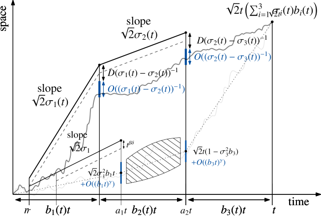
Figure 1. Localisation of an extremal particle of three-speed BBM in Case A. The dashed line depicts the effect of entropic repulsion.

4.2. Proof of Theorem 1.3.(i)

By Lemma 3.3 and Propositions 4.1, 4.2, and  4.3,

$${\mathbb{P}}\left(\max_{j\leq n(t)}\tilde{x}_{j}(t)-m^{+}(t)>y\right)$$

$$=\ {\mathbb{P}}\,\bigg{(}\exists_{i_{1}\leq n(b_{1}t),\dots,i_{\ell}\leq n^{\bar{i}_{\ell-1}}(b_{\ell}t)}\colon\bigg{\{}\sum_{k=1}^{\ell}\tilde{x}_{i_{k}}^{\,\bar{i}_{k-1}}(b_{k}t)-m^{+}(t)>y\bigg{\}}\land\bigg{\{}\tilde{x}_{i_{1}}\in{\mathcal{L}}_{b_{1}t,\sigma_{1},t^{\beta},B,D}\bigg{\}}$$

$$\qquad\land\bigg{\{}\forall_{1<k<\ell}\colon\tilde{x}_{i_{k}}^{\,\bar{i}_{k-1}}\in{\mathcal{L}}_{b_{k}t,\sigma_{k},B,D}^{\bar{i}_{k-1}}\bigg{\}}\bigg{)}+{\mathcal{O}}(\epsilon),$$ (4.58)

where

$${\mathcal{L}}_{b_{1}t,\sigma_{1},t^{\beta},B,D} \equiv{\mathcal{A}}_{t^{\beta},t^{\beta},t^{\beta\delta},\sigma_{1}}\cap{\mathcal{B}}_{t^{\beta},t^{\beta},0,\sigma_{1}}\cap{\mathcal{A}}_{t^{\beta},b_{1}t,t^{\beta\delta/2},\sigma_{1}}\cap{\mathcal{G}}_{b_{1}t,\sigma_{1},0,B,D},$$

$${\mathcal{L}}_{b_{k}t,\sigma_{k},B,D}^{\bar{i}_{k-1}} \equiv{\mathcal{A}}_{0,b_{k}t,t^{\beta\delta/2}-\Lambda^{\bar{i}_{k-1}}(t),\sigma_{k}}\cap{\mathcal{G}}_{b_{k}t,\sigma_{k},\Lambda^{\bar{i}_{k-1}}(t),B,D},$$ (4.59)

and

$${\mathcal{B}}_{r_{1},r_{2},S,\sigma}\equiv\left\{X\colon\forall_{r_{1}\leq s\leq r_{2}}\colon X(s)+S>-\sqrt{2}\sigma s\right\}.$$ (4.60)

Due to Lemma 3.7, it is enough to analyse

$${\mathbb{P}}\,\bigg{(}\max_{\begin{subarray}{c}i_{1}\leq n(b_{1}t)\colon\tilde{x}_{i_{1}}\in{\mathcal{L}}_{b_{1}t,\sigma_{1},t^{\beta},B,D},\dots,\\ i_{\ell}\leq n^{\bar{i}_{\ell-1}}(b_{\ell}t)\colon\tilde{x}_{i_{\ell}}^{\,\bar{i}_{\ell-1}}\in{\mathcal{L}}_{b_{\ell}t,\sigma_{\ell},B,D}^{\bar{i}_{\ell-1}}\end{subarray}}\,\sum_{k=1}^{\ell}\tilde{x}_{i_{k}}^{\,\bar{i}_{k-1}}(b_{k}t)-m^{+}(t)\leq y\bigg{)}$$

$$=\, {\mathbb{P}}\,\bigg{(}\max_{\begin{subarray}{c}i_{1}\leq n(b_{1}t)\\ \tilde{x}_{i_{1}}\in{\mathcal{L}}_{b_{1}t,\sigma_{1},t^{\beta},B,D}\end{subarray}}\ \max_{\begin{subarray}{c}\begin{subarray}{c}i_{2}\leq n^{i_{1}}(b_{2}t)\\ \tilde{x}_{i_{2}}^{\bar{i}_{1}}\in{\mathcal{L}}_{b_{2}t,\sigma_{2},B,D}^{\bar{i}_{1}}\end{subarray}\end{subarray}}\dots\max_{\begin{subarray}{c}i_{\ell}\leq n^{\bar{i}_{\ell-1}}(b_{\ell}t)\\ \tilde{x}_{i_{\ell}}^{\,\bar{i}_{\ell-1}}\in{\mathcal{L}}_{b_{\ell}t,\sigma_{\ell},B,D}^{\bar{i}_{\ell-1}}\end{subarray}}\sum_{k=1}^{\ell}\tilde{x}_{i_{k}}^{\,\bar{i}_{k-1}}(b_{k}t)-m^{+}(t)\leq y\bigg{)}.$$ (4.61)

Using the branching property, we rewrite this probability as

$${\mathbb{E}}\,\Bigg{[} \prod_{\begin{subarray}{c}i_{1}\leq n(b_{1}t)\\ \tilde{x}_{i_{1}}\in{\mathcal{L}}_{b_{1}t,\sigma_{1},t^{\beta},B,D}\end{subarray}}{\mathbb{E}}\,\Bigg{[}\prod_{\begin{subarray}{c}i_{2}\leq n^{i_{1}}(b_{2}t)\\ \tilde{x}_{i_{2}}^{\bar{i}_{1}}\in{\mathcal{L}}_{b_{2}t,\sigma_{2},B,D}^{\bar{i}_{1}}\end{subarray}}\dots\ {\mathbb{E}}\,\Bigg{[}\prod_{\begin{subarray}{c}i_{\ell-1}\leq n^{\bar{i}_{\ell-2}}(b_{\ell-1}t)\\ \tilde{x}_{i_{\ell-1}}^{\bar{i}_{\ell-2}}\in{\mathcal{L}}_{b_{\ell-1}t,\sigma_{\ell-1},B,D}^{\bar{i}_{\ell-2}}\end{subarray}}$$ (4.62)

$$\times\Bigg{(}1-{\mathbb{P}}\,\Bigg{(}\max_{i_{\ell}\leq n^{\bar{i}_{\ell-1}}(b_{\ell}t)}\tilde{x}_{i_{\ell}}^{\,\bar{i}_{\ell-1}}(b_{\ell}t)>m^{+}(t)-\sum_{k=1}^{\ell-1}\tilde{x}_{i_{k}}^{\,\bar{i}_{k-1}}(b_{k}t)+y\,\bigg{|}\,{\mathcal{F}}_{a_{\ell-1}t}\Bigg{)}\Bigg{)}\,\bigg{|}\,{\mathcal{F}}_{a_{\ell-2}t}\Bigg{]}\dots\bigg{|}\,{\mathcal{F}}_{a_{1}t}\Bigg{]}\Bigg{]}.$$

We compute this term from within, i.e. we first estimate the tail of the maximum with Proposition 3.1 and then iteratively compute the nested expectations. To apply the tail estimate, we need that $\Delta^{\bar{i}_{\ell-1}}(t)$ is positive and $\lim_{t\to\infty}\Delta^{\bar{i}_{\ell-1}}(t)/(b_{\ell}t)=0$, where

$$\Delta^{\bar{i}_{\ell-1}}(t) \equiv{\textstyle{\frac{1}{\sigma_{\ell}}}}\left(m^{+}(t)-\sum_{k=1}^{\ell-1}\tilde{x}_{i_{k}}^{\,\bar{i}_{k-1}}(b_{k}t)+y\right)-\left(\sqrt{2}b_{\ell}t-{\textstyle{\frac{3}{2\sqrt{2}}}}\ln(b_{\ell}t)\right)$$

$$={\textstyle{\frac{1}{\sigma_{\ell}}}}\left(\sum_{k=1}^{\ell-1}\sqrt{2}\sigma_{k}b_{k}t-\tilde{x}_{i_{k}}^{\,\bar{i}_{k-1}}(b_{k}t)\right)-{\textstyle{\frac{3}{2\sqrt{2}}}}\left(\sum_{k=1}^{\ell-1}\ln(b_{k}t)+2\ln(\sigma_{k}-\sigma_{k+1})\right)+y+o(1)$$

$$\equiv{\textstyle{\frac{1}{\sigma_{\ell}}}}\Lambda^{{\bar{i}_{\ell-1}}}(t)+L_{\ell-1}(t)+y+o(1)$$ (4.63)

and $L_{\ell-1}(t)$ is defined as in (4.37). Since $\tilde{x}_{i_{\ell-1}}^{\bar{i}_{\ell-2}}\in{\mathcal{L}}_{b_{\ell-1},\sigma_{\ell-1},B,D}^{\bar{i}_{\ell-2}}$, $\Delta^{\bar{i}_{\ell-1}}(t)=O\left((\sigma_{\ell-1}-\sigma_{\ell})^{-1}\right)$. By Assumption 1.1.(ii), $\Delta^{\bar{i}_{\ell-1}}(t)>0$, and by Assumption 1.1.(iii), $\lim_{t\to\infty}\Delta^{\bar{i}_{\ell-1}}(t)/(b_{\ell}t)=0$. Proposition 3.1 implies that

$${\mathbb{P}}\,\Bigg{(}\max_{i_{\ell}\leq n^{\bar{i}_{\ell-1}}(b_{\ell}t)}\tilde{x}_{i_{\ell}}^{\,\bar{i}_{\ell-1}}(b_{\ell}t)>m^{+}(t)-\sum_{k=1}^{\ell-1}\tilde{x}_{i_{k}}^{\,\bar{i}_{k-1}}(b_{k}t)+y\,\bigg{|}\,{\mathcal{F}}_{a_{\ell-1}t}\Bigg{)}$$

$$=\,C\Delta^{\bar{i}_{\ell-1}}(t){\mathrm{e}}^{-\sqrt{2}\Delta^{\bar{i}_{\ell-1}}(t)}(1+o(1)),$$ (4.64)

where $o(1)$ is uniform in the range of possible values of $\tilde{x}_{i_{\ell-1}}^{\,\bar{i}_{\ell-2}}$. Inserting (4.2) into (4.62), shows that the innermost expectation in (4.62) equals

$${\mathbb{E}}\,\Bigg{[}\prod_{\begin{subarray}{c}i_{\ell-1}\leq n^{\bar{i}_{\ell-2}}(b_{\ell-1}t)\\ \tilde{x}_{i_{\ell-1}}^{\bar{i}_{\ell-2}}\in{\mathcal{L}}_{b_{\ell-1}t,\sigma_{\ell-1},B,D}^{\bar{i}_{\ell-2}}\end{subarray}}\bigg{(}1-C\Delta^{\bar{i}_{\ell-1}}(t){\mathrm{e}}^{-\sqrt{2}\Delta^{\bar{i}_{\ell-1}}(t)}\bigg{)}\,\bigg{|}\,{\mathcal{F}}_{a_{\ell-2}t}\Bigg{]}(1+o(1))$$

$$=\, {\mathbb{E}}\,\Bigg{[}\exp\bigg{(}-\sum_{\begin{subarray}{c}i_{\ell-1}\leq n^{\bar{i}_{\ell-2}}(b_{\ell-1}t)\\ \tilde{x}_{i_{\ell-1}}^{\bar{i}_{\ell-2}}\in{\mathcal{L}}_{b_{\ell-1}t,\sigma_{\ell-1},B,D}^{\bar{i}_{\ell-2}}\end{subarray}}C\Delta^{\bar{i}_{\ell-1}}(t){\mathrm{e}}^{-\sqrt{2}\Delta^{\bar{i}_{\ell-1}}(t)}\bigg{)}\,\bigg{|}\,{\mathcal{F}}_{a_{\ell-2}t}\Bigg{]}(1+o(1)).$$ (4.65)

In the last step, we used $\Delta^{\bar{i}_{\ell-1}}(t)>\frac{D}{\sigma_{\ell-1}-\sigma_{\ell}}$ and therefore ${\mathrm{e}}^{-\sqrt{2}\Delta^{\bar{i}_{\ell-1}}(t)}\downarrow 0$, as $\uparrow\infty$.

We rewrite the right-hand side of (4.2) as

$${\mathbb{E}}\,\Bigg{[}\exp\bigg{(}-\sum_{\begin{subarray}{c}i_{\ell-1}\leq n^{\bar{i}_{\ell-2}}(b_{\ell-1}t),\\ \tilde{x}_{i_{\ell-1}}^{\bar{i}_{\ell-2}}\in{\mathcal{L}}_{b_{\ell-1}t,\sigma_{\ell-1},B,D}^{\bar{i}_{\ell-2}}\end{subarray}}C\Delta^{\bar{i}_{\ell-1}}(t){\mathrm{e}}^{-\sqrt{2}\Delta^{\bar{i}_{\ell-1}}(t)}\bigg{)}\,\bigg{|}\,{\mathcal{F}}_{a_{\ell-2}t}\Bigg{]}$$

$$=\, {\mathbb{E}}\,\Bigg{[}\exp\Bigg{(}-C{\mathrm{e}}^{-\sqrt{2}\,\left({\textstyle{\frac{1}{\sigma_{\ell}}}}\Lambda^{\bar{i}_{\ell-2}}(t)+L_{\ell-2}(t)+y\right)}\left(\frac{1}{\sigma_{\ell}}\Lambda^{\bar{i}_{\ell-2}}(t)\,{\mathcal{Y}}_{i_{\ell-2}}(t)+{\mathcal{Z}}_{i_{\ell-2}}(t)\right)\Bigg{)}\,\bigg{|}\,{\mathcal{F}}_{a_{\ell-2}t}\Bigg{]},$$ (4.66)

where

$${\mathcal{Y}}_{i_{\ell-2}}(t) \equiv\sum_{\begin{subarray}{c}i_{\ell-1}\leq n^{\bar{i}_{\ell-2}}(b_{\ell-1}t),\\ \tilde{x}_{i_{\ell-1}}^{\bar{i}_{\ell-2}}\in{\mathcal{L}}_{b_{\ell-1}t,\sigma_{\ell-1},B,D}^{\bar{i}_{\ell-2}}\end{subarray}}{\mathrm{e}}^{-\sqrt{2}\frac{1}{\sigma_{\ell}}\left(\sqrt{2}\sigma_{\ell-1}b_{\ell-1}t-\tilde{x}_{i_{\ell-1}}^{\bar{i}_{\ell-2}}(b_{\ell-1}t)\right)+\frac{3}{2}\big{(}\ln(b_{\ell-1}t)+2\ln(\sigma_{\ell-1}-\sigma_{\ell})\big{)}},$$ (4.67)

and

$${\mathcal{Z}}_{i_{\ell-2}}(t) \equiv\sum_{\begin{subarray}{c}i_{\ell-1}\leq n^{\bar{i}_{\ell-2}}(b_{\ell-1}t),\\ \tilde{x}_{i_{\ell-1}}^{\bar{i}_{\ell-2}}\in{\mathcal{L}}_{b_{\ell-1}t,\sigma_{\ell-1},B,D}^{\bar{i}_{\ell-2}}\end{subarray}}{\mathrm{e}}^{-\sqrt{2}\frac{1}{\sigma_{\ell}}\left(\sqrt{2}\sigma_{\ell-1}b_{\ell-1}t-\tilde{x}_{i_{\ell-1}}^{\bar{i}_{\ell-2}}(b_{\ell-1}t)\right)+\frac{3}{2}\big{(}\ln(b_{\ell-1}t)+2\ln(\sigma_{\ell-1}-\sigma_{\ell})\big{)}}$$

$$\hskip 79.6678pt\times\left({\textstyle{\frac{1}{\sigma_{\ell}}}}\left(\sqrt{2}\sigma_{\ell-1}b_{\ell-1}t-\tilde{x}_{i_{\ell-1}}^{\bar{i}_{\ell-2}}(b_{\ell-1}t)\right)+L_{\ell-1}(t)+y\right).$$ (4.68)

The exponential in (4.2) is well approximated by its linear approximation. To see this, we use the inequality

$$1-x\leq{\mathrm{e}}^{-x}\leq 1-x+\frac{x^{2}}{2},\quad x>0,$$ (4.69)

with

$$x=C{\mathrm{e}}^{-\sqrt{2}\,\left(\frac{1}{\sigma_{\ell}}\Lambda^{\bar{i}_{\ell-2}}(t)+L_{\ell-2}(t)+y\right)}\ \left({\textstyle{\frac{1}{\sigma_{\ell}}}}\Lambda^{\bar{i}_{\ell-2}}(t)\,{\mathcal{Y}}_{i_{\ell-2}}(t)+{\mathcal{Z}}_{i_{\ell-2}}(t)\right).$$ (4.70)

This gives the bounds

$$1-{\mathbb{E}}\left[x\,|\,{\mathcal{F}}_{a_{\ell-2}t}\right]\leq{\mathbb{E}}\left[{\mathrm{e}}^{-x}\,|\,{\mathcal{F}}_{a_{\ell-2}t}\right]\leq 1-{\mathbb{E}}\left[x\,|\,{\mathcal{F}}_{a_{\ell-2}t}\right]\left(1-\frac{1}{2}\frac{{\mathbb{E}}\left[x^{2}\,|\,{\mathcal{F}}_{a_{\ell-2}t}\right]}{{\mathbb{E}}\left[x\,|\,{\mathcal{F}}_{a_{\ell-2}t}\right]}\right).$$ (4.71)

The next two lemmas provide the necessary bounds on the conditional first and second moments of $x$. Their proofs are postponed to Subsection A.

Lemma 4.4.

For all $i_{1}\leq n(b_{1}t),\dots,i_{\ell-2}\leq n^{\bar{i}_{\ell-3}}(b_{\ell-2}t)$ with

$$\tilde{x}_{i_{1}}\in{\mathcal{L}}_{b_{1}t,\sigma_{1},t^{\beta},B,D},\dots,\tilde{x}_{i_{\ell-2}}^{\bar{i}_{\ell-3}}\in{\mathcal{L}}_{b_{\ell-2},\sigma_{\ell-2},B,D}^{\bar{i}_{\ell-3}},$$ (4.72)

$${\mathbb{E}}\,\Big{[}{\mathcal{Y}}_{i_{\ell-2}}(t)\,\big{|}\,{\mathcal{F}}_{a_{\ell-2}t}\Big{]} ={\textstyle{\frac{1}{\sqrt{\pi}}}}\Lambda^{\bar{i}_{\ell-2}}(t){\mathrm{e}}^{\sqrt{2}\Lambda^{\bar{i}_{\ell-2}}(t)\frac{\sigma_{\ell-1}-\sigma_{\ell}}{\sigma_{\ell-1}\sigma_{\ell}}}{\textstyle{\frac{\sigma_{\ell-1}-\sigma_{\ell}}{\sigma_{\ell-1}^{3}\sqrt{2}}}}\,(1+o(1)),$$ (4.73)

$${\mathbb{E}}\,\Big{[}{\mathcal{Z}}_{i_{\ell-2}}(t)\,\big{|}\,{\mathcal{F}}_{a_{\ell-2}t}\Big{]} ={\textstyle{\frac{1}{\sqrt{\pi}}}}\Lambda^{\bar{i}_{\ell-2}}(t){\mathrm{e}}^{\sqrt{2}\Lambda^{\bar{i}_{\ell-2}}(t)\frac{\sigma_{\ell-1}-\sigma_{\ell}}{\sigma_{\ell-1}\sigma_{\ell}}}\left({\textstyle{\frac{1}{\sigma_{\ell-1}^{3}\sigma_{\ell}}}}-\Lambda^{\bar{i}_{\ell-2}}(t){\textstyle{\frac{\sigma_{\ell-1}-\sigma_{\ell}}{\sigma_{\ell-1}^{3}\sigma_{\ell}\sqrt{2}}}}\right)\,(1+o(1)),$$

where $o(1)$ tends to $0$ as first $t\uparrow\infty$ and then $B\uparrow\infty,D\downarrow 0$.

To bound the conditional second moment of $x$, we write it as

$${\mathbb{E}}\left[x^{2}\,|\,{\mathcal{F}}_{a_{\ell-2}t}\right]$$

$$=\, C^{2}{\mathrm{e}}^{-2\sqrt{2}\,\left(\frac{1}{\sigma_{\ell}}\Lambda^{\bar{i}_{\ell-2}}(t)+L_{\ell-2}(t)+y\right)}\ {\mathbb{E}}\left[\left(\frac{1}{\sigma_{\ell}}\Lambda^{\bar{i}_{\ell-2}}(t)\,{\mathcal{Y}}_{i_{\ell-2}}(t)+{\mathcal{Z}}_{i_{\ell-2}}(t)\right)^{2}\bigg{|}\,{\mathcal{F}}_{a_{\ell-2}t}\right]$$

$$\leq\, C^{2}{\mathrm{e}}^{-2\sqrt{2}\,\left(\frac{1}{\sigma_{\ell}}\Lambda^{\bar{i}_{\ell-2}}(t)+L_{\ell-2}(t)+y\right)}\ {\mathbb{E}}\,\Bigg{[}\Bigg{(}\sum_{\begin{subarray}{c}i_{\ell-1}\leq n^{\bar{i}_{\ell-2}}(b_{\ell-1}t),\\ \tilde{x}_{i_{\ell-1}}^{\bar{i}_{\ell-2}}\in{\mathcal{L}}_{b_{\ell-1}t,\sigma_{\ell-1},B,D}^{\bar{i}_{\ell-2}}\end{subarray}}{\mathrm{e}}^{-\sqrt{2}\frac{1}{\sigma_{\ell}}\left(\sqrt{2}\sigma_{\ell-1}b_{\ell-1}t-\tilde{x}_{i_{\ell-1}}^{\bar{i}_{\ell-2}}(b_{\ell-1}t)\right)}\Bigg{)}^{2}\,\bigg{|}\,{\mathcal{F}}_{a_{\ell-2}t}\Bigg{]}$$

$$\times(b_{\ell-1}t)^{3}(\sigma_{\ell-1}-\sigma_{\ell})^{6}\left({\textstyle{\frac{B}{\sigma_{\ell}(\sigma_{\ell-1}-\sigma_{\ell})}}}+L_{\ell-1}(t)+y\right)^{2}.$$ (4.74)

In the last inequality, we bounded the non-exponential factors in ${\mathcal{Z}}_{i_{\ell-2}}(t)$ with the help of the localisation $\tilde{x}_{i_{\ell-1}}^{\bar{i}_{\ell-2}}\in{\mathcal{L}}_{b_{\ell-1}t,\sigma_{\ell-1},B,D}^{\bar{i}_{\ell-2}}$. By Assumption 1.1.(iii), the last line in (4.2) is at most of order $t^{3}$. The next lemma provides a bound on the expectation in (4.2).

Lemma 4.5.

For all $i_{1}\leq n(b_{1}t),\dots,i_{\ell-2}\leq n^{\bar{i}_{\ell-3}}(b_{\ell-2}t)$ as in Lemma 4.4

$${\mathbb{E}}\,\Bigg{[}\Bigg{(}\sum_{\begin{subarray}{c}i_{\ell-1}\leq n^{\bar{i}_{\ell-2}}(b_{\ell-1}t),\\ \tilde{x}_{i_{\ell-1}}^{\bar{i}_{\ell-2}}\in{\mathcal{L}}_{b_{\ell-1}t,\sigma_{\ell-1},B,D}^{\bar{i}_{\ell-2}}\end{subarray}}\exp\left({\textstyle-\sqrt{2}\frac{1}{\sigma_{\ell}}\left(\sqrt{2}\sigma_{\ell-1}b_{\ell-1}t-\tilde{x}_{i_{\ell-1}}^{\bar{i}_{\ell-2}}(b_{\ell-1}t)\right)}\right)\Bigg{)}^{2}\,\bigg{|}\,{\mathcal{F}}_{a_{\ell-2}t}\Bigg{]}$$

$$\leq\, P(t)\exp\left(-\tilde{C}t^{\beta}\right)\exp\left(\sqrt{2}\Lambda^{\bar{i}_{\ell-2}}(t)\left({\textstyle{\frac{\sigma_{\ell-1}-\sigma_{\ell}}{\sigma_{\ell-1}\sigma_{\ell}}}}+{\textstyle{\frac{1}{\sigma_{\ell}}}}\right)\right),$$ (4.75)

with $\tilde{C}>0$ a constant and $P$ is a function satisfying $P(t)\leq t^{c}$ for some $c>0$.

Comparing the first and second-order terms, we obtain with Lemma 4.4 and  4.5

$$\frac{{\mathbb{E}}\,\left[x^{2}\,\big{|}\,{\mathcal{F}}_{a_{\ell-2}t}\right]}{{\mathbb{E}}\,\left[x\,\big{|}\,{\mathcal{F}}_{a_{\ell-2}t}\right]}\leq\frac{1}{\Lambda^{\bar{i}_{\ell-2}}(t)}P(t){\mathrm{e}}^{-\tilde{C}t^{\beta}}\leq D(\sigma_{\ell-2}-\sigma_{\ell-1})P(t){\mathrm{e}}^{-\tilde{C}t^{\beta}}.$$ (4.76)

We used the localisation $x_{i_{\ell-2}}^{\bar{i}_{\ell-3}}\in{\mathcal{L}}_{b_{\ell-2}t,\sigma_{\ell-2}.B,D}^{\bar{i}_{\ell-3}}$ to bound $\Lambda^{\bar{i}_{\ell-2}}(t)$. By Assumption 1.1.(iii), the right-hand side of (4.76) converges to zero, as $t\uparrow\infty$. Together with (4.71), this yields

$${\mathbb{E}}\,\Big{[}{\mathrm{e}}^{-x}\,|\,{\mathcal{F}}_{a_{\ell-2}t}\Big{]}=\, \Big{(}1-{\mathbb{E}}\left[x\,|\,{\mathcal{F}}_{a_{\ell-2}t}\right]\Big{)}\,(1+o(1))$$

$$=\, \left(1-{\textstyle{\frac{C}{\sqrt{\pi}}}}\Lambda^{\bar{i}_{\ell-2}}(t){\mathrm{e}}^{-\sqrt{2}\,\left(\frac{1}{\sigma_{\ell-1}}\Lambda^{\bar{i}_{\ell-2}}(t)+L_{\ell-2}(t)+y\right)}\right)\,(1+o(1))$$

$$=\, \exp\left(-{\textstyle{\frac{C}{\sqrt{\pi}}}}\Lambda^{\bar{i}_{\ell-2}}(t){\mathrm{e}}^{-\sqrt{2}\,\left(\frac{1}{\sigma_{\ell-1}}\Lambda^{\bar{i}_{\ell-2}}(t)+L_{\ell-2}(t)+y\right)}\right)\,(1+o(1)).$$ (4.77)

The second equality follows from Lemma 4.4. In the third equality, we used (4.69) together with $\Lambda^{\bar{i}_{\ell-2}}(t)>D(\sigma_{\ell-2}-\sigma_{\ell-1})^{-1}$ and Assumption 1.1.(iii). Inserting (4.2) into the nested expectations in (4.62), the innermost expectation is equal to

$${\mathbb{E}}\,\Bigg{[}\exp\bigg{(}-\sum_{\begin{subarray}{c}i_{\ell-2}\leq n^{\bar{i}_{\ell-3}}(b_{\ell-2}t)\\ \tilde{x}_{i_{\ell-2}}^{\bar{i}_{\ell-3}}\in{\mathcal{L}}_{b_{\ell-2}t,\sigma_{\ell-2},B,D}^{\bar{i}_{\ell-3}}\end{subarray}}{\textstyle{\frac{C}{\sqrt{\pi}}}}\Lambda^{\bar{i}_{\ell-2}}(t){\mathrm{e}}^{-\sqrt{2}\,\left(\frac{1}{\sigma_{\ell-1}}\Lambda^{\bar{i}_{\ell-2}}(t)+L_{\ell-2}(t)+y\right)}\bigg{)}\,\bigg{|}\,{\mathcal{F}}_{a_{\ell-3}t}\Bigg{]}(1+o(1)).$$ (4.78)

This term almost looks like the left-hand side of (4.2). We can use the same arguments as in (4.2) – (4.2) to compute the remaining conditional expectations in (4.62) level by level. This leads to

$${\mathbb{E}}\,\Bigg{[}\prod_{\begin{subarray}{c}i_{1}\leq n(b_{1}t),\\ \tilde{x}_{i_{1}}\in{\mathcal{L}}_{b_{1}t,\sigma_{1},t^{\beta},B,D}\end{subarray}} \exp\,\bigg{(}{-}{\textstyle{\frac{C}{\pi^{(\ell-2)/2}}}}{\mathrm{e}}^{-\sqrt{2}y}\,\bigr{(}\sqrt{2}\sigma_{1}b_{1}t-\tilde{x}_{i_{1}}(b_{1}t)\bigr{)}$$

$$\times{\mathrm{e}}^{-\sqrt{2}\frac{1}{\sigma_{1}}\left(\sqrt{2}\sigma_{1}b_{1}t-\tilde{x}_{i_{1}}(b_{1}t)\right)+\frac{3}{2}\big{(}\ln(b_{1}t)+2\ln(\sigma_{1}-\sigma_{2})\big{)}}\bigg{)}\Bigg{]}(1+o(1)).$$ (4.79)

To compute the expectation, we split the range of integration $[0,b_{1}t)$ into $[0,t^{\beta})$ and $[t^{\beta},b_{1}t)$, and abbreviate the length of the second part by $t^{*}\equiv b_{1}t-t^{\beta}$. We choose $\beta\in(0,1/2)$ such that Assumption 1.1.(iii) is satisfied. Denote by $\{\tilde{x}_{j}(t^{\beta})\colon 1\leq j\leq n(t^{\beta})\}$ the particles of a BBM with variance $\sigma_{1}^{2}$ at time $t^{\beta}$, and, for each $j$, denote by $\{\tilde{x}_{j^{*}}^{j}(t^{*})\colon 1\leq j^{*}\leq n(t^{*})\}$ the particles of independent BBMs with variance $\sigma_{1}^{2}$ at time $t^{*}$. We set

$$\widetilde{{\mathcal{L}}}_{t^{*},\sigma_{1},\tilde{x}_{j}\left(t^{\beta}\right)-\sqrt{2}\sigma_{1}t^{\beta},B,D} \equiv{\mathcal{A}}_{0,t^{*},t^{\beta\delta/2}+\tilde{x}_{j}\left(t^{\beta}\right)-\sqrt{2}\sigma_{1}t^{\beta},\sigma_{1}}\cap{\mathcal{G}}_{t^{*},\sigma_{1},\tilde{x}_{j}(t^{\beta})-\sqrt{2}\sigma_{1}t^{\beta},B,D},$$

$$\widetilde{{\mathcal{L}}}_{t^{\beta},t^{\beta\delta},\sigma_{1}} \equiv{\mathcal{A}}_{t^{\beta},t^{\beta},t^{\beta\delta},\sigma_{1}}\cap{\mathcal{B}}_{t^{\beta},t^{\beta},0,\sigma_{1}}.$$ (4.80)

By conditioning on ${\mathcal{F}}_{t^{\beta}}$, we rewrite (4.2) as

$${\mathbb{E}}\,\Bigg{[}\prod_{\begin{subarray}{c}j\leq n(t^{\beta})\\ \tilde{x}_{j}\in\widetilde{{\mathcal{L}}}_{t^{\beta},t^{\beta\delta},\sigma_{1}}\end{subarray}}{\mathbb{E}}\, \Bigg{[}\exp\bigg{(}-{\textstyle{\frac{C}{\pi^{(\ell-2)/2}}}}{\mathrm{e}}^{-\sqrt{2}\,\left(\frac{1}{\sigma_{2}}\left(\sqrt{2}\sigma_{1}t^{\beta}-\tilde{x}_{j}\left(t^{\beta}\right)\right)+y\right)}$$

$$\times\left(\left(\sqrt{2}\sigma_{1}t^{\beta}-\tilde{x}_{j}\left(t^{\beta}\right)\right)\widetilde{{\mathcal{Y}}}_{j}(t)+\widetilde{{\mathcal{Z}}}_{j}(t)\right)\bigg{)}\,\bigg{|}\,{\mathcal{F}}_{t^{\beta}}\Bigg{]}\Bigg{]}(1+o(1)),$$ (4.81)

where

$$\widetilde{{\mathcal{Y}}}_{j}(t) \equiv\sum_{\begin{subarray}{c}j^{*}\leq n^{j}(t^{*}),\\ \tilde{x}_{j^{*}}^{\,j}\in\widetilde{{\mathcal{L}}}_{t^{*},\sigma_{1},\tilde{x}_{j}(t^{\beta})-\sqrt{2}\sigma_{1}t^{\beta},B,D}\end{subarray}}{\mathrm{e}}^{-\sqrt{2}\,\frac{1}{\sigma_{2}}\left(\sqrt{2}\sigma_{1}t^{*}-\tilde{x}_{j^{*}}^{\,j}(t^{*})\right)+\frac{3}{2}\big{(}\ln(b_{1}t)+2\ln(\sigma_{1}-\sigma_{2})\big{)}},$$

$$\widetilde{{\mathcal{Z}}}_{j}(t) \equiv\sum_{\begin{subarray}{c}j^{*}\leq n^{j}(t^{*}),\\ \tilde{x}_{j^{*}}^{\,j}\in\widetilde{{\mathcal{L}}}_{t^{*},\sigma_{1},\tilde{x}_{j}(t^{\beta})-\sqrt{2}\sigma_{1}t^{\beta},B,D}\end{subarray}}\left(\sqrt{2}\sigma_{1}t^{*}-x_{j^{*}}^{\,j}(t^{*})\right){\mathrm{e}}^{-\sqrt{2}\frac{1}{\sigma_{2}}\left(\sqrt{2}\sigma_{1}t^{*}-\tilde{x}_{j^{*}}^{\,j}(t^{*})\right)+\frac{3}{2}\big{(}\ln(b_{1}t)+2\ln(\sigma_{1}-\sigma_{2})\big{)}}.$$ (4.82)

The proofs of the following lemmas are very similar to the corresponding results in [8] and use the same technique as in (4.2) – (4.2). We give the details in Appendix A for completeness. We set

$$z={\textstyle{\frac{C}{\pi^{(\ell-2)/2}}}}{\mathrm{e}}^{-\sqrt{2}\,\left(\frac{1}{\sigma_{2}}\left(\sqrt{2}\sigma_{1}t^{\beta}-\tilde{x}_{j}\left(t^{\beta}\right)\right)+y\right)}\left(\left(\sqrt{2}\sigma_{1}t^{\beta}-\tilde{x}_{j}(t^{\beta})\right)\widetilde{{\mathcal{Y}}}_{j}(t)+\widetilde{{\mathcal{Z}}}_{j}(t)\right).$$ (4.83)

In the first step, we compute the first moments of $\widetilde{{\mathcal{Y}}}_{j}(t)$ and $\widetilde{{\mathcal{Z}}}_{j}(t)$.

Lemma 4.6.

For all $j\leq n(t^{\beta})$ with $\tilde{x}_{j}\in{\mathcal{L}}_{r,t^{\beta},t^{\beta\delta},\sigma_{1}}$,

$${\mathbb{E}}\,\Big{[}\widetilde{{\mathcal{Y}}}_{j}(t)\,|\,{\mathcal{F}}_{t^{\beta}}\Big{]} ={\textstyle{\frac{1}{\sqrt{\pi}}}}\left(\sqrt{2}\sigma_{1}t^{\beta}-\tilde{x}_{j}(t^{\beta})\right){\textstyle{\frac{\sigma_{1}-\sigma_{2}}{\sigma_{1}^{3}\sqrt{2}}}}(1+o(1)),$$ (4.84)

$${\mathbb{E}}\,\Big{[}\widetilde{{\mathcal{Z}}}_{j}(t)\,|\,{\mathcal{F}}_{t^{\beta}}\Big{]} ={\textstyle{\frac{1}{\sqrt{\pi}}}}\left(\sqrt{2}\sigma_{1}t^{\beta}-\tilde{x}_{j}(t^{\beta})\right){\textstyle{\frac{1}{\sigma_{1}^{3}}}}\left(1-\left(\sqrt{2}\sigma_{1}t^{\beta}-\tilde{x}_{j}(t^{\beta})\right){\textstyle{\frac{\sigma_{1}-\sigma_{2}}{\sqrt{2}}}}\right)(1+o(1)),$$

where $o(1)$ tends to $0$ as first $t\uparrow\infty$ and then $B\uparrow\infty,D\downarrow 0$.

We bound ${\mathbb{E}}[z^{2}\,|\,{\mathcal{F}}_{t^{\beta}}]$ from above by

$${\mathrm{e}}^{-2\sqrt{2}\,\left(\frac{1}{\sigma_{2}}\left(\sqrt{2}\sigma_{1}t^{\beta}-\tilde{x}_{j}\left(t^{\beta}\right)\right)+y\right)}\ {\mathbb{E}}\,\bigg{[}\bigg{(}\sum_{\begin{subarray}{c}j^{*}\leq n^{j}(t^{*}),\\ \tilde{x}_{j^{*}}^{\,j}\in\widetilde{{\mathcal{L}}}_{t^{*},\sigma_{1},\tilde{x}_{j}(t^{\beta})-\sqrt{2}\sigma_{1}t^{\beta},B,D}\end{subarray}}\exp\left({\textstyle-\sqrt{2}\frac{1}{\sigma_{2}}\left(\sqrt{2}\sigma_{1}t^{*}-\tilde{x}_{j^{*}}^{\,j}(t^{*})\right)}\right)\bigg{)}^{2}\,\Big{|}\,{\mathcal{F}}_{t^{\beta}}\bigg{]}$$

$$\times{\textstyle{\frac{C^{2}}{\pi^{(\ell-2)}}}}(b_{1}t)^{3}(\sigma_{1}-\sigma_{2})^{6}\left(\left(\sqrt{2}\sigma_{1}t^{\beta}-\tilde{x}_{j}(t^{\beta})\right)+{\textstyle{\frac{B}{\sigma_{1}-\sigma_{2}}}}\right)^{2},$$ (4.85)

where we used the localisation $\tilde{x}_{j^{*}}^{\,j}\in\widetilde{{\mathcal{L}}}_{t^{*},\sigma_{1},\tilde{x}_{j}(t^{\beta})-\sqrt{2}\sigma_{1}t^{\beta},B,D}$ to bound the non-exponential factors in $\widetilde{{\mathcal{Z}}}_{j}(t)$ by $(\sigma_{1}-\sigma_{2})^{-1}B$. Due to $\tilde{x}_{j}\in{\mathcal{L}}_{t^{\beta},t^{\beta\delta},\sigma_{1}}$, $\sqrt{2}\sigma_{1}t^{\beta}-\tilde{x}_{j}(t^{\beta})\in(t^{\beta\delta},2\sqrt{2}t^{\beta})$. Together with Assumption 1.1.(iii), we see that the last line in (4.2) is bounded by $C^{2}t^{3+2\beta}$. It remains to estimate the conditional expectation in the right-hand side of (4.2):

Lemma 4.7.

For all $j\leq n(t^{\beta})$ with $\tilde{x}_{j}\in{\mathcal{L}}_{r,t^{\beta},t^{\beta\delta},\sigma_{1}}$,

$${\mathbb{E}}\,\bigg{[}\bigg{(}\sum_{\begin{subarray}{c}j^{*}\leq n^{j}(t^{*}),\\ \tilde{x}_{j^{*}}^{\,j}\in\widetilde{{\mathcal{L}}}_{t^{*},\sigma_{1},\tilde{x}_{j}(t^{\beta})-\sqrt{2}\sigma_{1}t^{\beta},B,D}\end{subarray}}\exp\left({\textstyle-\sqrt{2}\frac{1}{\sigma_{2}}\left(\sqrt{2}\sigma_{1}t^{*}-\tilde{x}_{j^{*}}^{\,j}(t^{*})\right)}\right)\bigg{)}^{2}\,\bigg{|}\,{\mathcal{F}}_{t^{\beta}}\bigg{]}\leq\,P(t)\exp\left(-\tilde{C}t^{\beta}\right),$$ (4.86)

where we use the notation from Lemma 4.5.

Comparing the first and second moments terms of $z$, we obtain with Lemma 4.6 and 4.7

$$\frac{{\mathbb{E}}\left[z^{2}\,\big{|}\,{\mathcal{F}}_{t^{\beta}}\right]}{{\mathbb{E}}\left[z\,\big{|}\,{\mathcal{F}}_{t^{\beta}}\right]}\leq\frac{1}{\sqrt{2}\sigma_{1}t^{\beta}-\tilde{x}_{j}\left(t^{\beta}\right)}P(t){\mathrm{e}}^{-\tilde{C}t^{\beta}}\leq t^{-\beta\delta}P(t){\mathrm{e}}^{-\tilde{C}t^{\beta}}.$$ (4.87)

The upper bound is due to $\tilde{x}_{j}\in{\mathcal{L}}_{t^{\beta},t^{\beta\delta},\sigma_{1}}$ and converges to zero as $t\uparrow\infty$. Next, we approximate ${\mathbb{E}}\left[{\mathrm{e}}^{-z}\,|\,{\mathcal{F}}_{t^{\beta}}\right]$ as in (4.2):

$${\mathbb{E}}\,\Big{[}{\mathrm{e}}^{-z}\,\Big{|}\,{\mathcal{F}}_{t^{\beta}}\Big{]}=\, \exp\Bigg{(}-{\textstyle{\frac{C}{\pi^{(\ell-1)/2}}}}\left(\sqrt{2}\sigma_{1}t^{\beta}-\tilde{x}_{j}(t^{\beta})\right){\mathrm{e}}^{-\sqrt{2}\,\left(\frac{1}{\sigma_{2}}\left(\sqrt{2}\sigma_{1}t^{\beta}-\tilde{x}_{j}\left(t^{\beta}\right)-t^{\beta\delta}\right)+y\right)}\Bigg{)}\,(1+o(1)).$$ (4.88)

Inserting the right-hand side of (4.88) into (4.2), we see that (4.2) is equal to

$${\mathbb{E}}\,\Bigg{[}\exp\Bigg{(}-{\textstyle{\frac{C}{\pi^{(\ell-1)/2}}}}{\mathrm{e}}^{-\sqrt{2}y}\sum_{\begin{subarray}{c}j\leq n(t^{\beta})\\ \tilde{x}_{j}\in\widetilde{{\mathcal{L}}}_{t^{\beta},t^{\beta\delta},\sigma_{1}}\end{subarray}}\left(\sqrt{2}\sigma_{1}t^{\beta}-\tilde{x}_{j}(t^{\beta})\right){\mathrm{e}}^{-\sqrt{2}\frac{1}{\sigma_{2}}\left(\sqrt{2}\sigma_{1}t^{\beta}-\tilde{x}_{j}\left(t^{\beta}\right)\right)}\Bigg{)}\Bigg{]}(1+o(1)).$$ (4.89)

Finally, the sum in (4.89) converges to the limit of the derivative martingale.

Lemma 4.8.

With the notation above,

$$\sum_{j\leq n(t^{\beta})}\mathbbm{1}_{\left\{\tilde{x}_{j}\in\widetilde{{\mathcal{L}}}_{t^{\beta},t^{\beta\delta},\sigma_{1}}\right\}}\left(\sqrt{2}\sigma_{1}t^{\beta}-\tilde{x}_{j}(t^{\beta})\right){\mathrm{e}}^{-\sqrt{2}\frac{1}{\sigma_{2}}\left(\sqrt{2}\sigma_{1}t^{\beta}-\tilde{x}_{j}\left(t^{\beta}\right)\right)}\to Z,$$ (4.90)

in probability, as $t\uparrow\infty$, where $Z$ is the limit of the derivative martingale.

Proof.

This follows as the proof of [8, Lemma 3.7], except that the exact asymptotic behaviour of $\sigma_{1}/\sigma_{2}$, is replaced by the relation $t^{\beta}\ll(\sigma_{1}-\sigma_{2})^{-1}$. ∎

Due to Lemma 4.8 and $Z>0$ a.s., (4.89) converges to

$${\mathbb{E}}\left[\exp\left(-{\textstyle{\frac{C}{\pi^{(\ell-1)/2}}}}Z{\mathrm{e}}^{-\sqrt{2}y}\right)\right],$$ (4.91)

as $t\uparrow\infty$. This proves Part (i) of Theorem 1.3.

5. The limiting extremal distribution in Case B

In this section, we prove Part (ii) of Theorem 1.3. We begin with the case of $\ell$-speed BBM and write $\alpha_{1},\alpha_{\ell}$ instead of $\alpha_{\mathrm{begin}},\alpha_{\mathrm{end}}$, and $b_{1},b_{\ell}$ instead of $b_{\mathrm{begin}},b_{\mathrm{end}}$ to be consistent with Case A.

Assumption 5.1.

Let $\alpha_{1},\alpha_{\ell}\in\left(0,1/2\right)$. We assume that the family of covariance functions $\left(A_{t}\right)_{t>0}$ with $A_{t}(s)<s$ for all $t>0,s\in(0,1)$, satisfies:

1. The functions $(A_{t})_{t>0}$ are piecewise linear and continuous: Their derivatives are given by

   $$A_{t}^{\prime}(s)=\sum_{k=1}^{\ell}\sigma_{k}^{2}\mathbbm{1}_{\left(\sum_{j=1}^{k-1}b_{j},\sum_{j=1}^{k}b_{j}\right)}(s),$$ (5.1)

   with velocities $\sigma_{k}\colon{\mathbb{R}}_{+}\to{\mathbb{R}}_{+},1\leq k\leq\ell,$ and interval lengths $b_{k}\colon{\mathbb{R}}_{+}\to(0,1]$, $1\leq k\leq\ell$. We assume for all $t>0$ that $\sum_{k=1}^{\ell}b_{k}=1$ and $\sum_{k=1}^{\ell}\sigma_{k}^{2}b_{k}=1$.

2. The velocity on the first interval satisfies $\sigma_{1}^{2}=1-t^{-\alpha_{1}}+o(t^{-\alpha_{1}})$ and the interval length $b_{1}$ satisfies $1\gg b_{1}\gg t^{\alpha_{1}-1/2}$ as $t\uparrow\infty$.

3. The velocity on the last interval satisfies $\sigma_{\ell}^{2}=1+t^{-\alpha_{\ell}}+o(t^{-\alpha_{\ell}})$ and the interval length $b_{\ell}$ satisfies $1\gg b_{\ell}\gg t^{\alpha_{\ell}-1/2}$ as $t\uparrow\infty$.

4. Minimum distance to the identity function: $\min_{s\in[b_{1},1-b_{\ell}]}\big{(}s-A_{t}(s)\big{)}\gg t^{-1/2}$ as $t\uparrow\infty$.

From now on, we write $(\bar{X}_{t})_{t>0}$ for $\ell$-speed BBM with covariance functions $(A_{t})_{t>0}$ satisfying Assumption 5.1.

Proposition 5.2.

Let $C$ be the positive constant from Proposition 3.1 and denote by $Z$ the limit of the derivative martingale. Then, for all $y\in{\mathbb{R}}$,

$$\lim_{t\uparrow\infty}{\mathbb{P}}\left(\max_{j\leq n(t)}\bar{x}_{j}(t)-m^{-}(t)\leq y\right)={\mathbb{E}}_{Z}\left[{\mathrm{e}}^{-CZ{\mathrm{e}}^{-\sqrt{2}y}}\right],$$ (5.2)

where

$$m^{-}(t)=\sqrt{2}t-{\textstyle{\frac{1+2(\alpha_{1}+\alpha_{\ell})}{2\sqrt{2}}}}\ln(t).$$ (5.3)

5.1. Localisation

We define the sets

$${\mathcal{T}}_{r_{1},r_{2},S,\gamma}\equiv\bigg{\{}X\colon\forall_{r_{1}\leq s\leq r_{2}}\colon\big{|}X(s)+S-\sqrt{2}tA_{t}\left(s/t\right)\big{|}<\Big{(}A_{t}\left(s/t\right)\wedge\big{(}1-A_{t}\left(s/t\right)\!\big{)}\Big{)}^{\gamma}t^{\gamma}\bigg{\}}.$$ (5.4)

Between times $b_{1}t$ and $(1-b_{\ell})t$, extremal particles fluctuate like a time-inhomogeneous Brownian bridge with time-inhomogeneity controlled by the covariance function.

Proposition 5.3 (Fluctuations in the middle part).

For any $y\in{\mathbb{R}}$, any $\epsilon>0$, any $\gamma>1/2$ and for all $t$ large enough,

$${\mathbb{P}}\,\bigg{(} \exists_{j\leq n(t)}\colon\Big{\{}\bar{x}_{j}(t)>m^{-}(t)-y\Big{\}}\land\,\bigg{\{}\bar{x}_{j}\not\in{\mathcal{T}}_{b_{1}t,(1-b_{\ell})t,0,\gamma}\bigg{)}<\epsilon.$$ (5.5)

We first control the localisation at the times of the first and last speed change.

Lemma 5.4 (Position at the last speed change).

For any $y\in{\mathbb{R}}$, any $\epsilon>0$, any $\gamma>1/2$ and for all $t$ large enough,

$${\mathbb{P}}\,\bigg{(} \exists_{j\leq n(t)}\colon\Big{\{}\bar{x}_{j}(t)>m^{-}(t)-y\Big{\}}\land\,\bigg{\{}\left|\bar{x}_{j}((1-b_{\ell})t)-\sqrt{2}(1-\sigma_{\ell}^{2}b_{\ell})t\right|>(\sigma_{\ell}^{2}b_{\ell}t)^{\gamma}\bigg{\}}\bigg{)}<\epsilon.$$ (5.6)

Lemma 5.5 (Position at the first speed change).

For any $y\in{\mathbb{R}}$, any $\epsilon>0$, any $\gamma>1/2$ and for all $t$ large enough,

$${\mathbb{P}}\,\bigg{(} \exists_{j\leq n(t)}\colon\Big{\{}\bar{x}_{j}(t)>m^{-}(t)-y\Big{\}}\land\,\bigg{\{}\left|\bar{x}_{j}(b_{1}t)-\sqrt{2}\sigma_{1}^{2}b_{1}t\right|>(\sigma_{1}^{2}b_{1}t)^{\gamma}\bigg{\}}\bigg{)}<\epsilon.$$ (5.7)

Proof of Lemma 5.4.

A first moment method as in (4.1) – (4.1) shows that the probability in (5.6) is bounded from above by

$${\mathrm{e}}^{(1-b_{\ell})t}\int_{J_{1}}{\textstyle{\frac{\mathrm{d}\omega}{\sqrt{2\pi(1-\sigma_{\ell}^{2}b_{\ell})t}}}}{\mathrm{e}}^{-{\textstyle{\frac{\omega^{2}}{2(1-\sigma_{\ell}^{2}b_{\ell})t}}}}{\mathbb{P}}\,\bigg{(}\max_{i\leq n(b_{\ell}t)}\sigma_{\ell}x_{i}^{b_{\ell}t}(b_{\ell}t)>m^{-}(t)-\omega-y\,\bigg{)},$$ (5.8)

where $\left(x_{i}^{b_{\ell}t}(b_{\ell}t)\right)_{i\leq n(b_{\ell}t)}$ denotes a standard BBM at time $b_{\ell}t$ and

$$J_{1} \equiv\left(-\infty,\sqrt{2}(1-\sigma_{\ell}^{2}b_{\ell})t-(\sigma_{\ell}^{2}b_{\ell}t)^{\gamma}\right)\cup\left(\sqrt{2}(1-\sigma_{\ell}^{2}b_{\ell})t+(\sigma_{\ell}^{2}b_{\ell}t)^{\gamma},\infty\right),$$ (5.9)

We split the range of integration $J_{1}$ into $\Big{[}\!\sqrt{2}(1-b_{\ell})t,\infty\Big{)}$ and $J_{2}\equiv J_{1}\setminus\Big{[}\!\sqrt{2}(1-b_{\ell})t,\infty\Big{)}$.
For $\omega\in\left[\!\sqrt{2}(1-b_{\ell})t,\infty\right)$, we bound the probability in (5.8) by $1$ and the integral by

$${\mathrm{e}}^{(1-b_{\ell})t}\int_{\sqrt{2}(1-b_{\ell})t}^{\infty}{\textstyle{\frac{\mathrm{d}\omega}{\sqrt{2\pi(1-\sigma_{\ell}^{2}b_{\ell})t}}}}{\mathrm{e}}^{-{\textstyle{\frac{\omega^{2}}{2(1-\sigma_{\ell}^{2}b_{\ell})t}}}}\leq{\mathrm{e}}^{(1-b_{\ell})t}{\mathrm{e}}^{-{\textstyle{\frac{(1-b_{\ell})^{2}t}{(1-\sigma_{\ell}^{2}b_{\ell})}}}}=o(1),$$ (5.10)

by a Gaussian tail bound. For the integral over $J_{2}$, we write

$$z(t,\omega)\equiv\sigma_{\ell}^{-1}\left(m^{-}(t)-\omega-y\right)-\sqrt{2}b_{\ell}t,$$ (5.11)

and use [8, Lemma 2.3] to get

$$\begin{split}{\mathbb{P}}\,\bigg{(}\max_{i\leq n(b_{\ell}t)}\sigma_{\ell}x_{i}^{b_{\ell}t}(b_{\ell}t)>m^{-}(t)-\omega-y\,\bigg{)}&\leq{\textstyle{\frac{1}{\sqrt{2\pi}(\sqrt{2b_{\ell}t}+z(t,\omega)/\!\sqrt{b_{\ell}t})}}}{\mathrm{e}}^{-\sqrt{2}z(t,\omega)-{\textstyle{\frac{z^{2}(t,\omega)}{2b_{\ell}t}}}}\\ &\leq{\textstyle{\frac{1}{2\sqrt{\pi b_{\ell}t}}}}{\mathrm{e}}^{b_{\ell}t-{\textstyle{\frac{\left(m^{-}(t)-\omega-y\right)^{2}}{2\sigma_{\ell}^{2}b_{\ell}t}}}}(1+o(1)).\end{split}$$ (5.12)

By (5.10) and (5.12), (5.8) is not larger than

$${\textstyle{\frac{1}{2\sqrt{\pi b_{\ell}t}}}}{\mathrm{e}}^{t}\int_{J_{2}}{\textstyle{\frac{\mathrm{d}\omega}{\sqrt{2\pi(1-\sigma_{\ell}^{2}b_{\ell})t}}}}{\mathrm{e}}^{-{\textstyle{\frac{\omega^{2}}{2(1-\sigma_{\ell}^{2}b_{\ell})t}}}}{\mathrm{e}}^{-{\textstyle{\frac{\left(m^{-}(t)-\omega+-\right)^{2}}{2\sigma_{\ell}^{2}b_{\ell}t}}}}(1+o(1))$$

$$=\> {\textstyle{\frac{1}{2\sqrt{\pi b_{\ell}t}}}}{\mathrm{e}}^{t-{\textstyle{\frac{(m^{-}(t)-y)^{2}}{2t}}}}\int_{J_{2}}{\textstyle{\frac{\mathrm{d}\omega}{\sqrt{2\pi(1-\sigma_{\ell}^{2}b_{\ell})t}}}}\exp\left(-{\textstyle{\frac{\left(\omega\,-\,(1-\sigma_{\ell}^{2}b_{\ell})(m^{-}(t)-y)\right)^{2}}{2(1-\sigma_{\ell}^{2}b_{\ell})\,\sigma_{\ell}^{2}b_{\ell}t}}}\right)(1+o(1))$$

$$=\> {\textstyle{\frac{{\mathrm{e}}^{\sqrt{2}d}\,t^{1/2+\alpha_{1}+\alpha_{\ell}}}{\sqrt{b_{\ell}}}}}\!\!\!\int\limits_{\left(-(\sigma_{\ell}^{2}b_{\ell}t)^{\gamma}\!,\,(\sigma_{\ell}^{2}b_{\ell}t)^{\gamma}\right)^{c}}\!{\textstyle{\frac{\mathrm{d}\omega}{\sqrt{2\pi(1-\sigma_{\ell}^{2}b_{\ell})t}}}}\exp\Bigg{(}{-}{\textstyle{\frac{\left(\omega\,-\,(1-\sigma_{\ell}^{2}b_{\ell})\left(m^{-}(t)\,-\!\sqrt{2}t-y\right)\right)^{2}}{2(1-\sigma_{\ell}^{2}b_{\ell})\,\sigma_{\ell}^{2}b_{\ell}t}}}\Bigg{)}(1+o(1)),$$ (5.13)

which tends to zero as $t\uparrow\infty$ since $m^{-}(t)\,-\!\sqrt{2}t-y={\mathcal{O}}(\ln(t))$. ∎

Proof of Lemma 5.5.

Due to Assumption 5.1.(iii), we can choose $\gamma>1/2$ such that

$$1\gg b_{\ell} \gg t^{\frac{\alpha_{\ell}+\gamma-1}{1-\gamma}}.$$ (5.14)

By Lemma 5.4, the probability in (5.7) equals

$${\mathbb{P}}\,\bigg{(}\exists_{j\leq n(t)}\colon\Big{\{}\bar{x}_{j}(t)>m^{-}(t)-y\Big{\}}\land\,\bigg{\{}\left|\bar{x}_{j}(b_{1}t)-\sqrt{2}\sigma_{1}^{2}b_{1}t\right|>(\sigma_{1}^{2}b_{1}t)^{\gamma}\bigg{\}}$$

$$\quad\quad\qquad\land\,\bigg{\{}\left|\bar{x}_{j}((1-b_{\ell})t)-\sqrt{2}(1-\sigma_{\ell}^{2}b_{\ell})t\right|\leq(\sigma_{\ell}^{2}b_{\ell}t)^{\gamma}\bigg{\}}\bigg{)}+{\mathcal{O}}(\epsilon)$$

$$\leq\> {\mathrm{e}}^{(1-b_{\ell})t}\!\!\displaystyle\int\limits_{(I_{1})^{c}}\!\!\!\!{\textstyle{\frac{\mathrm{d}\omega_{1}}{\sqrt{2\pi\sigma_{1}^{2}b_{1}t}}}}{\mathrm{e}}^{-{\textstyle{\frac{\omega_{1}^{2}}{2\sigma_{1}^{2}b_{1}t}}}}\int\limits_{I_{2}}\!\!\!\!{\textstyle{\frac{\mathrm{d}\omega_{2}}{\sqrt{2\pi(1-\sigma_{1}^{2}b_{1}-\sigma_{\ell}^{2}b_{\ell})t}}}}{\mathrm{e}}^{-{\textstyle{\frac{\omega_{2}^{2}}{2(1-\sigma_{1}^{2}b_{1}-\sigma_{\ell}^{2}b_{\ell})t}}}}$$

$$\quad\quad\qquad\times{\mathbb{P}}\,\bigg{(}\max_{i\leq n(b_{\ell}t)}\sigma_{\ell}x_{i}^{b_{\ell}t}(b_{\ell}t)>m^{-}(t)-\omega_{1}-\omega_{2}-y\bigg{)}+{\mathcal{O}}(\epsilon),$$ (5.15)

where

$$I_{1} \equiv\left(\sqrt{2}\sigma_{1}^{2}b_{1}t-(\sigma_{1}^{2}b_{1}t)^{\gamma},\sqrt{2}\sigma_{1}^{2}b_{1}t+(\sigma_{1}^{2}b_{1}t)^{\gamma}\right),$$

$$I_{2} \equiv\left(\sqrt{2}(1-\sigma_{\ell}^{2}b_{\ell})t-\omega_{1}-(\sigma_{\ell}^{2}b_{\ell}t)^{\gamma},\sqrt{2}(1-\sigma_{\ell}^{2}b_{\ell})t-\omega_{1}+(\sigma_{\ell}^{2}b_{\ell}t)^{\gamma}\right).$$ (5.16)

For $\omega_{2}\in I_{2}$, by (5.14), we can use 3.1 and get

$${\mathbb{P}}\,\bigg{(}\max_{i\leq n(b_{\ell}t)}\sigma_{\ell}x_{i}^{b_{\ell}t}(b_{\ell}t)>m^{-}(t)-\omega_{1}-\omega_{2}-y\,\bigg{)}={\textstyle{\frac{C}{\sqrt{2}}}}b_{\ell}t^{1-\alpha_{\ell}}{\mathrm{e}}^{b_{\ell}t-{\textstyle{\frac{\left(\sqrt{2}t-\omega_{1}-\omega_{2}+L(t)-y\right)^{2}}{2\sigma_{\ell}^{2}b_{\ell}t}}}}(1+o(1)),$$ (5.17)

where

$$L(t)\equiv{\textstyle{\frac{3}{2\sqrt{2}}}}\sigma_{\ell}\ln(b_{\ell}t)-{\textstyle{\frac{1+2(\alpha_{1}+\alpha_{\ell})}{2\sqrt{2}}}}\ln(t).$$ (5.18)

This implies that

$$\int\limits_{I_{2}}\!\!\!\!{\textstyle{\frac{\mathrm{d}\omega_{2}}{\sqrt{2\pi(1-\sigma_{1}^{2}b_{1}-\sigma_{\ell}^{2}b_{\ell})t}}}}{\mathrm{e}}^{-{\textstyle{\frac{\omega_{2}^{2}}{2(1-\sigma_{1}^{2}b_{1}-\sigma_{\ell}^{2}b_{\ell})t}}}}{\mathbb{P}}\,\bigg{(}\max_{i\leq n(b_{\ell}t)}\sigma_{\ell}x_{i}^{b_{\ell}t}(b_{\ell}t)>m^{-}(t)-\omega_{1}-\omega_{2}-y\,\bigg{)}$$

$$={\textstyle{\frac{C}{\sqrt{2}}}}b_{\ell}t^{1-\alpha_{\ell}}{\mathrm{e}}^{b_{\ell}t}{\mathrm{e}}^{-{\textstyle{\frac{\left(\sqrt{2}t-\omega_{1}+L(t)-y\right)^{2}}{2(1-\sigma_{1}^{2}b_{1})t}}}}\int\limits_{I_{2}}{\textstyle{\frac{\mathrm{d}\omega_{2}}{\sqrt{2\pi(1-\sigma_{1}^{2}b_{1}-\sigma_{\ell}^{2}b_{\ell})t}}}}$$

$$\qquad\times\exp\Bigg{(}{-}(1-\sigma_{1}^{2}b_{1}){\textstyle{\frac{\left(\omega_{2}-\left(1-\sigma_{1}^{2}b_{1}\right)^{-1}\left(1-\sigma_{1}^{2}b_{1}-\sigma_{\ell}^{2}b_{\ell}\right)\left(\sqrt{2}t-\omega_{1}+L(t)-y\right)\right)^{2}}{2(1-\sigma_{1}^{2}b_{1}-\sigma_{\ell}^{2}b_{\ell})\sigma_{\ell}^{2}b_{\ell}t}}}\Bigg{)}(1+o(1))$$

$$\leq{\textstyle{\frac{C}{\sqrt{2}}}}b_{\ell}t^{1-\alpha_{\ell}}{\mathrm{e}}^{b_{\ell}t}{\mathrm{e}}^{-{\textstyle{\frac{\left(\sqrt{2}t-\omega_{1}+L(t)-y\right)^{2}}{2(1-\sigma_{1}^{2}b_{1})t}}}}{\textstyle{\frac{\sigma_{\ell}b_{\ell}^{1/2}}{(1-\sigma_{1}^{2}b_{1})^{1/2}}}}(1+o(1)).$$ (5.19)

Therefore, (5.15) is not larger than

$$\begin{split}&{\textstyle{\frac{C}{\sqrt{2}}}}b_{\ell}^{3/2}t^{1-\alpha_{\ell}}{\mathrm{e}}^{-\sqrt{2}(L(t)-y)-\frac{(L(t)-y)^{2}}{2t}}\int\limits_{\left(-(\sigma_{1}^{2}b_{1}t)^{\gamma}\!,\,(\sigma_{1}^{2}b_{1}t)^{\gamma}\right)^{c}}{\textstyle{\frac{\mathrm{d}\omega_{1}}{\sqrt{2\pi(1-\sigma_{1}^{2}b_{1})\sigma_{1}^{2}b_{1}t}}}}\exp\left(-{\textstyle{\frac{\left(\omega_{1}-\sigma_{1}^{2}b_{1}(L(t)-y)\right)^{2}}{2(1-\sigma_{1}^{2}b_{1})\sigma_{1}^{2}b_{1}t}}}\right)(1+o(1)).\end{split}$$ (5.20)

The prefactor is of polynomial order and the integral is of order $\exp\left(-\frac{(b_{1}t)^{2\gamma-1}}{2}\right)$. By Assumption 5.1.(ii), (5.20) tends to zero as $t\uparrow\infty$. ∎

Proof of Proposition 5.3.

Let $\gamma$ be close enough to $1/2$ such that (5.14) as well as

$$1\gg b_{1} \gg t^{\frac{\alpha_{1}+\gamma-1}{1-\gamma}}$$ (5.21)

are satisfied. Choose $\tilde{\gamma}$ s.t. $1/2<\tilde{\gamma}<\gamma$ and $\tilde{\gamma}<1$. By Lemmas 3.3, 5.4, and 5.5, the probability in (5.5) is equal to

$${\mathbb{P}}\,\bigg{(} \exists_{j\leq n(t)}\colon\Big{\{}\bar{x}_{j}(t)>m^{-}(t)-y\Big{\}}\land\,\left\{\bar{x}_{j}\in{\mathcal{A}}_{r,b_{1}t,0,\sigma_{1}}\cap{\mathcal{T}}_{b_{1}t,b_{1}t,0,\tilde{\gamma}}\cap{\mathcal{T}}_{(1-b_{\ell})t,(1-b_{\ell})t,0,\tilde{\gamma}}\right\}$$

$$\land\,\bigg{\{}\exists_{b_{1}t\leq s\leq(1-b_{\ell})t}\colon\big{|}\bar{x}_{j}(s)-\sqrt{2}tA_{t}(s/t)\big{|}>\Big{(}A_{t}(s/t)\wedge\big{(}1-A_{t}(s/t)\!\big{)}\Big{)}^{\gamma}t^{\gamma}\bigg{\}}\bigg{)}+{\mathcal{O}}(\epsilon),$$ (5.22)

for $r,t>0$ large enough. As in (4.1) – (4.1), we see that the probability in (5.1) is bounded from above by

$${\mathrm{e}}^{(1-b_{\ell})t}\,{\mathbb{E}}\bigg{[}\mathbbm{1}_{\bar{x}^{t}_{1}\in{\mathcal{A}}_{r,b_{1}t,0,\sigma_{1}}\cap{\mathcal{T}}_{b_{1}t,b_{1}t,0,\tilde{\gamma}}}\,{\mathbb{E}}\bigg{[}\mathbbm{1}_{\bar{x}^{t}_{1}\in{\mathcal{T}}_{(1-b_{\ell})t,(1-b_{\ell})t,0,\tilde{\gamma}}}\mathbbm{1}_{\exists_{b_{1}t\leq s\leq(1-b_{\ell})t}\colon|\bar{x}^{t}_{1}(s)-\sqrt{2}tA_{t}(s/t)|>\left(A_{t}(s/t)\wedge\left(1-A_{t}(s/t)\!\right)\right)^{\gamma}t^{\gamma}}$$

$$\quad\times{\mathbb{P}}\,\bigg{(}\max_{i\leq n(b_{\ell}t)}\sigma_{\ell}x_{i}^{b_{\ell}t}(b_{\ell}t)>m^{-}(t)-\bar{x}^{t}_{1}((1-b_{\ell})t)-y\,\bigg{|}\,{\mathcal{F}}_{(1-b_{\ell})t}\bigg{)}\bigg{|}\,{\mathcal{F}}_{b_{1}t}\bigg{]}\bigg{]}$$

$$=\> {\mathrm{e}}^{(1-b_{\ell})t}\!\!\displaystyle\int\limits_{I_{1}}\!\!{\textstyle{\frac{\mathrm{d}\omega_{1}}{\sqrt{2\pi\sigma_{1}^{2}b_{1}t}}}}{\mathrm{e}}^{-{\textstyle{\frac{\omega_{1}^{2}}{2\sigma_{1}^{2}b_{1}t}}}}\ {\mathbb{P}}\,\bigg{(}{\mathfrak{z}}_{0,\frac{\omega_{1}}{\sigma_{1}}}^{b_{1}t}(s)\leq\!\sqrt{2}s\,\forall\!_{s\in[r,b_{1}t]}\bigg{)}\displaystyle\int\limits_{I_{2}}\!\!{\textstyle{\frac{\mathrm{d}\omega_{2}}{\sqrt{2\pi(1-\sigma_{1}^{2}b_{1}-\sigma_{\ell}^{2}b_{\ell})t}}}}{\mathrm{e}}^{-{\textstyle{\frac{\omega_{2}^{2}}{2(1-\sigma_{1}^{2}b_{1}-\sigma_{\ell}^{2}b_{\ell})t}}}}$$

$$\quad\quad\times{\mathbb{P}}\left(\exists_{s\in[b_{1}t,(1-b_{\ell})t]}\colon\!\left|{\mathfrak{z}}_{\omega_{1},\omega_{1}+\omega_{2}}^{(1-\sigma_{1}^{2}b_{1}-\sigma_{\ell}^{2}b_{\ell})t}\scriptstyle\left(A_{t}(s/t)t-\sigma_{1}^{2}b_{1}t\right)\>-\sqrt{2}tA_{t}(s/t)\right|\scriptstyle\,>\,\left(A_{t}(s/t)\wedge\left(1-A_{t}(s/t)\right)\right)^{\gamma}t^{\gamma}\!\right)$$

$$\quad\quad\times{\mathbb{P}}\,\bigg{(}\max_{i\leq n(b_{\ell}t)}\sigma_{\ell}x_{i}^{b_{\ell}t}(b_{\ell}t)>m^{-}(t)-\omega_{1}-\omega_{2}-y\,\bigg{)},$$ (5.23)

with $I_{1},I_{2}$ as in (5.1). We first bound the probabilities involving Brownian bridges. As in (4.13), for $\gamma>1/2$ and $\omega_{1}\in I_{1}$,

$${\mathbb{P}}\,\bigg{(}{\mathfrak{z}}_{0,{\textstyle{\frac{\omega_{1}}{\sigma_{1}}}}}^{b_{1}t}(s)\leq\!\sqrt{2}s\,\forall\!_{s\in[r,b_{1}t]}\bigg{)} \leq{\textstyle{\frac{2\sqrt{r}}{b_{1}t-r}}}\left(\sqrt{2}b_{1}t-{\textstyle{\frac{\omega_{1}}{\sigma_{1}}}}\right)(1+o(1))$$

$$\leq 2\sqrt{r}\left(\sqrt{2}(1-\sigma_{1})+\sigma_{1}^{2\gamma}b_{1}t^{1-\gamma}\right)(1+o(1))$$

$$=\sqrt{2r}t^{-\alpha_{1}}(1+o(1)).$$ (5.24)

For the second probability involving a bridge, the term inside the absolute value equals

$${\mathfrak{z}}_{0,0}^{(1-\sigma_{1}^{2}b_{1}-\sigma_{\ell}^{2}b_{\ell})t}\left(A_{t}(s/t)t-\sigma_{1}^{2}b_{1}t\right)+\omega_{1}+{\textstyle{\frac{A_{t}(s/t)-\sigma_{1}^{2}b_{1}}{1-\sigma_{1}^{2}b_{1}-\sigma_{\ell}^{2}b_{\ell}}}}\omega_{2}-\sqrt{2}tA_{t}(s/t).$$ (5.25)

For each $s\in[b_{1}t,(1-b_{\ell})t]$ and $\omega_{1},\omega_{2}$ in the ranges of integration,

$$\omega_{1}+{\textstyle{\frac{A_{t}(s/t)-\sigma_{1}^{2}b_{1}}{1-\sigma_{1}^{2}b_{1}-\sigma_{\ell}^{2}b_{\ell}}}}\omega_{2}-\sqrt{2}tA_{t}(s/t)=\>O\left({\textstyle{\frac{1-\sigma_{\ell}^{2}b_{\ell}-A_{t}(s/t)}{1-\sigma_{1}^{2}b_{1}-\sigma_{\ell}^{2}b_{\ell}}}}(b_{1}t)^{\tilde{\gamma}}+{\textstyle{\frac{A_{t}(s/t)-\sigma_{1}^{2}b_{1}}{1-\sigma_{1}^{2}b_{1}-\sigma_{\ell}^{2}b_{\ell}}}}(\sigma_{\ell}^{2}b_{\ell}t)^{\tilde{\gamma}}\right).$$ (5.26)

We will show that, for $s\in[b_{1}t,(1-b_{\ell})t]$ and $t$ large enough,

$${\textstyle{\frac{1-\sigma_{\ell}^{2}b_{\ell}-A_{t}(s/t)}{1-\sigma_{1}^{2}b_{1}-\sigma_{\ell}^{2}b_{\ell}}}}(\sigma_{1}^{2}b_{1}t)^{\tilde{\gamma}}+{\textstyle{\frac{A_{t}(s/t)-\sigma_{1}^{2}b_{1}}{1-\sigma_{1}^{2}b_{1}-\sigma_{\ell}^{2}b_{\ell}}}}(\sigma_{\ell}^{2}b_{\ell}t)^{\tilde{\gamma}}\leq\big{(}A_{t}(s/t)\wedge\left(1-A_{t}(s/t)\right)\!\big{)}^{\tilde{\gamma}}t^{\tilde{\gamma}}(1+o(1)).$$ (5.27)

Namely, (5.27) holds for $s=b_{1}t$ and $s=(1-b_{\ell})t$. Assumptions 5.1.(ii)–(iii) imply that(5.27) holds for $s$ s.t. $A_{t}(s/t)=1/2$. Concavity of $x\mapsto x^{\tilde{\gamma}}$ on ${\mathbb{R}}_{+}$ and monotonicity of $A_{t}$ imply that (5.27) holds for all $s\in[b_{1}t,(1-b_{\ell})t]$, and so for those $s$, (5.25) equals

$${\mathfrak{z}}_{0,0}^{(1-\sigma_{1}^{2}b_{1}-\sigma_{\ell}^{2}b_{\ell})t}\left(A_{t}(s/t)t-\sigma_{1}^{2}b_{1}t\right)+o\Big{(}\big{(}A_{t}(s/t)\wedge\left(1-A_{t}(s/t)\right)\!\big{)}^{\gamma}t^{\gamma}\Big{)}.$$ (5.28)

Thus the one-but-last probability in (5.23) is bounded from above by

$$\begin{split}&{\mathbb{P}}\left(\exists_{s\in[b_{1}t,(1-b_{\ell})t]}\colon\!\left|{\mathfrak{z}}^{(1-\sigma_{1}^{2}b_{1}-\sigma_{\ell}b_{\ell})t}_{0,0}\scriptstyle\left(A_{t}(s/t)t-\sigma_{1}^{2}b_{1}t\right)\right|\scriptstyle\,>\,\left(A_{t}(s/t)\wedge\left(1-A_{t}(s/t)\right)\!\right)^{\gamma}t^{\gamma}\right)(1+o(1)).\end{split}$$ (5.29)

The fluctuations of the Brownian bridge in (5.29) are bounded by those of $\Big{(}{\mathfrak{z}}^{t}_{0,0}\left(A_{t}(s/t)t\right)\!\Big{)}_{s\in[0,t]}$ for $s\in[b_{1}t,(1-b_{\ell})t]$, and thus (5.29) is bounded by

$${\mathbb{P}}\left(\exists_{s\in[b_{1}t,(1-b_{\ell})t]}\colon\!\left|{\mathfrak{z}}^{t}_{0,0}\scriptstyle\left(A_{t}(s/t)t\right)\right|\scriptstyle\,>\,\left(A_{t}(s/t)\wedge\left(1-A_{t}(s/t)\right)\!\right)^{\gamma}t^{\gamma}\right)(1+o(1)).$$ (5.30)

This probability is by the monotonicity of $A_{t}$ not larger than

$${\mathbb{P}}\left(\exists_{s\in[\tilde{r},t-\tilde{r}]}\colon\!\left|{\mathfrak{z}}^{t}_{0,0}\big{(}s\big{)}\right|\,>\,\big{(}s\wedge\left(t-s\right)\!\big{)}^{\gamma}\right)\leq\epsilon\sqrt{2\pi}/(C\sqrt{r}),$$ (5.31)

for $\tilde{r},t>0$ large enough, by 3.5. With (5.24) and (5.31) we see that (5.23) is smaller than

$$\epsilon{\textstyle{\frac{\sqrt{2}}{C}}}t^{-\alpha_{1}}{\mathrm{e}}^{(1-b_{\ell})t}\!\!\displaystyle\int\limits_{I_{1}}\!\! {\textstyle{\frac{\mathrm{d}\omega_{1}}{\sqrt{2\pi\sigma_{1}^{2}b_{1}t}}}}{\mathrm{e}}^{-\frac{\omega_{1}^{2}}{2\sigma_{1}^{2}b_{1}t}}\!\int\limits_{I_{2}}{\textstyle{\frac{\mathrm{d}\omega_{2}}{\sqrt{2\pi(1-\sigma_{1}^{2}b_{1}-\sigma_{\ell}^{2}b_{\ell})t}}}}{\mathrm{e}}^{-\frac{\omega_{2}^{2}}{2(1-\sigma_{1}^{2}b_{1}-\sigma_{\ell}^{2}b_{\ell})t}}$$

$$\times{\mathbb{P}}\,\bigg{(}\max_{i\leq n(b_{\ell}t)}\sigma_{\ell}x_{i}^{b_{\ell}t}(b_{\ell}t)>m^{-}(t)-\omega_{1}-\omega_{2}-y\,\bigg{)}(1+o(1)).$$ (5.32)

For $\omega_{1}\in I_{1}$ and $\tilde{\gamma}>1/2$, the bound in (5.1) is asymptotically sharp, and so the integral over $\omega_{2}$ in (5.32) is equal to

$${\textstyle{\frac{C}{\sqrt{2(1-\sigma_{1}^{2}b_{1})}}}}b_{\ell}^{3/2}t^{1-\alpha_{\ell}}{\mathrm{e}}^{b_{\ell}t}\exp\left(-{\textstyle{\frac{\left(\sqrt{2}t-\omega_{1}+L(t)-y\right)^{2}}{2(1-\sigma_{1}^{2}b_{1})t}}}\right)(1+o(1)).$$ (5.33)

Inserting (5.33) into (5.32) and shifting $\omega_{1}$ by $\sqrt{2}\sigma_{1}^{2}b_{1}t$, we see that (5.32) is equal to

$$\begin{split}&\epsilon b_{\ell}^{3/2}t^{1-\alpha_{1}-\alpha_{\ell}}{\mathrm{e}}^{t}{\mathrm{e}}^{-\frac{(\sqrt{2}t+L(t)-y)^{2}}{2t}}\!\!\displaystyle\int\limits_{-(\sigma_{1}^{2}b_{1}t)^{\tilde{\gamma}}\!}^{\,(\sigma_{1}^{2}b_{1}t)^{\tilde{\gamma}}}\!\!\!{\textstyle{\frac{\mathrm{d}\omega_{1}}{\sqrt{2\pi(1-\sigma_{1}^{2}b_{1})\sigma_{1}^{2}b_{1}t}}}}\exp\left({-}{\textstyle{\frac{\left(\omega_{1}-\sigma_{1}^{2}b_{1}(L(t)-y)\right)^{2}}{2(1-\sigma_{1}^{2}b_{1})\sigma_{1}^{2}b_{1}t}}}\right)(1+o(1)).\end{split}$$ (5.34)

Note that the integrands in (5.20) and (5.34) are the same, but the ranges of integration are complementary. We have seen that the integral in (5.20) tends to zero as $t\uparrow\infty$, which implies that the Gaussian integral in (5.34) tends to one. Recalling the definition of $L(t)$ in (5.18), we find that the $t$-dependent factors outside the integral in (5.34) tend to one as well, from which the claim follows. ∎

The next proposition is the analog to Proposition 4.3. It describes the effect of entropic repulsion on the first time interval $[0,b_{1}t]$ for extremal particles.

Proposition 5.6 (Entropic repulsion).

Let $0<\beta<\alpha_{1}$. Then, for any $y\in{\mathbb{R}}$ and for any $\epsilon>0$, there exists a constant $\delta\in(0,1/2)$ such that, for all $t$ large enough,

$$\begin{split}{\mathbb{P}}\,\bigg{(}&\exists_{j\leq n(t)}\colon\Big{\{}\bar{x}_{j}(t)>m^{-}(t)-y\Big{\}}\land\,\bigg{\{}\exists_{t^{\beta}\leq s\leq b_{1}t}\colon\bar{x}_{j}(s)>\sqrt{2}\sigma_{1}s-t^{\beta\delta}\bigg{\}}\bigg{)}<\epsilon.\end{split}$$ (5.35)

This means that the extremal particles of $(\bar{X}_{t})_{t>0}$ lie in ${\mathcal{A}}_{t^{\beta},b_{1}t,t^{\beta\delta},\sigma_{1}}$ with high probability. By monotonicity, we can use the superset ${\mathcal{A}}_{t^{\beta},t^{\beta},t^{\beta\delta},\sigma_{1}}\cap{\mathcal{A}}_{t^{\beta},b_{1}t,t^{\beta\delta/2},\sigma_{1}}$ of ${\mathcal{A}}_{t^{\beta},b_{1}t,t^{\beta\delta},\sigma_{1}}$ instead.

Proof.

Let $\gamma>1/2$ be close enough to $1/2$ that (5.14) and (5.21) are satisfied. By Lemmas 3.3, 5.4 and 5.5, the probability in (5.35) is equal to

$${\mathbb{P}}\,\bigg{(} \exists_{j\leq n(t)}\colon\Big{\{}\bar{x}_{j}(t)>m^{-}(t)-y\Big{\}}\land\,\left\{\bar{x}_{j}\in{\mathcal{T}}_{b_{1}t,b_{1}t,0,\gamma}\cap{\mathcal{T}}_{(1-b_{\ell})t,(1-b_{\ell})t,0,\gamma}\cap{\mathcal{A}}_{r,b_{1}t,0,\sigma_{1}}\right\}$$

$$\land\,\bigg{\{}\bar{x}_{j}(t^{\beta})>-\sqrt{2}\sigma_{1}t^{\beta}\bigg{\}}\land\,\bigg{\{}\exists_{t^{\beta}\leq s\leq b_{1}t}\colon\bar{x}_{j}(s)>\sqrt{2}\sigma_{1}s-t^{\beta\delta}\bigg{\}}\bigg{)}+{\mathcal{O}}(\epsilon),$$ (5.36)

for $r,t>0$ large enough. As in (4.1), we see that the probability in (5.1) is bounded from above by

$${\mathrm{e}}^{(1-b_{\ell})t}\int\limits_{I_{1}}\!\!{\textstyle{\frac{\mathrm{d}\omega_{1}}{\sqrt{2\pi\sigma_{1}^{2}(b_{1}t)}}}}{\mathrm{e}}^{-{\textstyle{\frac{\omega_{1}^{2}}{2\sigma_{1}^{2}(b_{1}t)}}}}\int\limits_{I_{2}}{\textstyle{\frac{\mathrm{d}\omega_{2}}{\sqrt{2\pi(1-\sigma_{1}^{2}b_{1}-\sigma_{\ell}^{2}b_{\ell})t}}}}{\mathrm{e}}^{-{\textstyle{\frac{\omega_{2}^{2}}{2(1-\sigma_{1}^{2}b_{1}-\sigma_{\ell}^{2}b_{\ell})t}}}}$$

$$\times\Bigg{[}{\mathbb{P}}\,\Big{(}{\mathfrak{z}}_{0,\frac{\omega_{1}}{\sigma_{1}}-\sqrt{2}b_{1}t}^{b_{1}t}(s)\leq 0\,\forall_{s\in[r,b_{1}t]}\Big{)}-{\mathbb{P}}\,\Big{(}{\mathfrak{z}}_{0,\frac{\omega_{1}}{\sigma_{1}}-\sqrt{2}b_{1}t}^{b_{1}t}(s)\leq-{\textstyle{\frac{t^{\beta\delta}}{\sigma_{1}}}}\,\forall_{s\in[t^{\beta},b_{1}t]}\Big{)}\Bigg{]}$$

$$\times{\mathbb{P}}\,\bigg{(}\max_{i\leq n(b_{\ell}t)}\sigma_{\ell}x_{i}^{b_{\ell}t}(b_{\ell}t)>m^{-}(t)-\omega_{1}-\omega_{2}-y\,\bigg{)},$$ (5.37)

with $I_{1},I_{2}$ as in (5.1). We have seen in (5.32)–(5.34) that replacing the difference of probabilities in (5.1) with $t^{-\alpha_{1}}$ creates a term of order $1$. Thus, it suffices to show that

$${\mathbb{P}}\,\Big{(}{\mathfrak{z}}_{0,\frac{\omega_{1}}{\sigma_{1}}-\sqrt{2}b_{1}t}^{b_{1}t}(s)\leq 0\,\forall_{s\in[r,b_{1}t]}\Big{)}-{\mathbb{P}}\,\Big{(}{\mathfrak{z}}_{0,\frac{\omega_{1}}{\sigma_{1}}-\sqrt{2}b_{1}t}^{b_{1}t}(s)\leq-{\textstyle{\frac{t^{\beta\delta}}{\sigma_{1}}}}\,\forall_{s\in[t^{\beta},b_{1}t]}\Big{)}\ll t^{-\alpha_{1}}.$$ (5.38)

We deal with the difference of probabilities in (5.1) as in (4.52)–(4.57). The only difference is that we replace $\frac{y_{1}}{\sigma_{1}(\sigma_{1}-\sigma_{2})}$ by $\sqrt{2}b_{1}t-\frac{\omega_{1}}{\sigma_{1}}$ and use that for $\omega_{1}$ from the integral in (5.1),

$${\textstyle{\frac{\sqrt{2}b_{1}t-\sigma_{1}^{-1}\omega_{1}}{b_{1}t-t^{\beta}}}}=2^{-1/2}t^{-\alpha_{1}}(1+o(1)).$$ (5.39)

Then we get that the difference of probabilities in (5.1) is not larger than a term of order

$$\sqrt{r}\,t^{\beta(\delta-1/2)}{\textstyle{\frac{\sqrt{2}b_{1}t-\sigma_{1}^{-1}\omega_{1}}{b_{1}t-t^{\beta}}}}\ll t^{-\alpha_{1}}.$$ (5.40)

In the last step, we applied (5.39) again and used that $\delta<1/2$. ∎

In Figure 2, we illustrate the localisation results in the case of $3$-speed VSBBM.

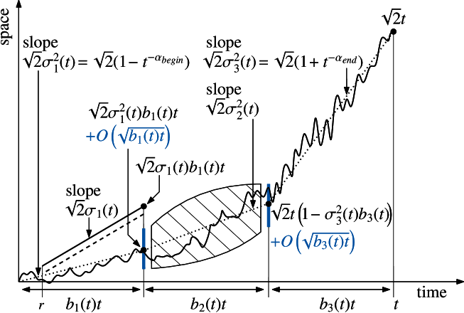
Figure 2. Localisation of an extremal particle of three-speed BBM in Case B. The dotted line depicts the function $\sqrt{2}A_{t}(s/t)t$ for $s\in[0,t]$. The dashed box depicts fluctuations of order $\sqrt{\min\{A_{t}(s/t)t,t-A_{t}(s/t)t\}}$. The dashed line depicts the effect of entropic repulsion.

5.2. Proof of Proposition 5.2

The structure of this proof is identical to that of Theorem 1.3.(i).

Let $\epsilon>0$, $r>0$, $\gamma>1/2$ and $0<\beta<\alpha_{1}$ be such that $t^{\beta}\ll b_{1}t$. Lemma 3.3 and Propositions 5.3 and 5.6 imply that

$${\mathbb{P}}\,\bigg{(}\exists_{j\leq n(t)}\colon\Big{\{}\bar{x}_{j}(t)>m^{-}(t)-y\Big{\}}\land\,\bigg{\{}\bar{x}_{j}\notin{\mathcal{L}}\bigg{\}}\bigg{)}<\epsilon,$$ (5.41)

for all $r,t$ large enough, where

$${\mathcal{L}} ={\mathcal{L}}_{b_{1}t}\cap{\mathcal{T}}_{b_{1}t,(1-b_{\ell})t,0,\gamma},$$

$${\mathcal{L}}_{b_{1}t} ={\mathcal{B}}_{t^{\beta},t^{\beta},0,\sigma_{1}}\cap{\mathcal{A}}_{t^{\beta},t^{\beta},t^{\beta\delta},\sigma_{1}}\cap{\mathcal{A}}_{t^{\beta},b_{1}t,t^{\beta\delta/2},\sigma_{1}}\cap{\mathcal{T}}_{b_{1}t,b_{1}t,0,\gamma},$$ (5.42)

recalling

$${\mathcal{A}}_{r_{1},r_{2},S,\sigma} =\left\{X\colon\forall_{r_{1}\leq s\leq r_{2}}\colon X(s)+S\leq\sqrt{2}\sigma s\right\},$$

$${\mathcal{B}}_{r_{1},r_{2},S,\sigma} =\left\{X\colon\forall_{r_{1}\leq s\leq r_{2}}\colon X(s)+S>-\sqrt{2}\sigma s\right\}.$$ (5.43)

By 3.7, Proposition 5.2 will follow from

$$\lim_{t\uparrow\infty}{\mathbb{P}}\left(\max_{j\leq n(t)\colon\bar{x}_{j}\in{\mathcal{L}}}\bar{x}_{j}(t)-m^{-}(t)\leq y\right)={\mathbb{E}}_{Z}\Big{[}\exp\Big{(}{-}CZ{\mathrm{e}}^{-\sqrt{2}y}\Big{)}\Big{]}.$$ (5.44)

Proceeding as in (4.2)–(4.62), we write the probability in (5.44) as

$${\mathbb{E}}\,\Bigg{[}\prod_{\begin{subarray}{c}i_{1}\leq n(b_{1}t),\\ \bar{x}_{i_{1}}\in{\mathcal{L}}_{b_{1}t}\end{subarray}}{\mathbb{E}}\,\Bigg{[}\prod_{\begin{subarray}{c}i_{2}\leq n^{i_{1}}(b_{2}t),\dots,i_{\ell-1}\leq n^{\bar{i}_{\ell-2}}(b_{\ell-1}t),\\ \sum_{k=1}^{\ell-1}\bar{x}_{i_{k}}^{\,\bar{i}_{k-1}}\in{\mathcal{T}}_{b_{1}t,(1-b_{\ell})t,0,\gamma}\end{subarray}}$$

$$\qquad\times\Bigg{(}1-{\mathbb{P}}\,\Bigg{(}\max_{i_{\ell}\leq n^{\bar{i}_{\ell-1}}(b_{\ell}t)}\bar{x}_{i_{\ell}}^{\,\bar{i}_{\ell-1}}(b_{\ell}t)>m^{-}(t)-\sum_{k=1}^{\ell-1}\bar{x}_{i_{k}}^{\,\bar{i}_{k-1}}(b_{k}t)+y\,\bigg{|}\,{\mathcal{F}}_{(1-b_{\ell})t}\Bigg{)}\Bigg{)}\,\bigg{|}\,{\mathcal{F}}_{b_{1}t}\Bigg{]}\Bigg{]}.$$ (5.45)

Since $\sum_{k=1}^{\ell-1}\bar{x}_{i_{k}}^{\,\bar{i}_{k-1}}\in{\mathcal{T}}_{b_{1}t,(1-b_{\ell})t,0,\gamma}$, the F-KPP asymptotics from 3.1 imply

$${\mathbb{P}}\, \Bigg{(}\max_{i_{\ell}\leq n^{\bar{i}_{\ell-1}}(b_{\ell}t)}\bar{x}_{i_{\ell}}^{\,\bar{i}_{\ell-1}}(b_{\ell}t)>m^{-}(t)-\sum_{k=1}^{\ell-1}\bar{x}_{i_{k}}^{\,\bar{i}_{k-1}}(b_{k}t)+y\,\bigg{|}\,{\mathcal{F}}_{(1-b_{\ell})t}\Bigg{)}$$

$$=\> C\Delta^{\bar{i}_{\ell-1}}(t)\exp\left(b_{\ell}t-{\textstyle{\frac{\left(\Delta^{\bar{i}_{\ell-1}}(t)+\sqrt{2}b_{\ell}t\right)^{2}}{2b_{\ell}t}}}\right)(1+o(1)),$$ (5.46)

with

$$\Delta^{\bar{i}_{\ell-1}}(t)\equiv{\textstyle{\frac{1}{\sigma_{\ell}}}}\left(m^{-}(t)-\sum\limits_{k=1}^{\ell-1}\bar{x}_{i_{k}}^{\,\bar{i}_{k-1}}(b_{k}t)+y\right)-\left(\sqrt{2}b_{\ell}t-{\textstyle{\frac{3}{2\sqrt{2}}}}\ln(b_{\ell}t)\right).$$ (5.47)

Inserting (5.46) into (5.45) yields

$${\mathbb{E}}\, \Bigg{[}\!\prod_{\begin{subarray}{c}i_{2}\leq n^{i_{1}}(b_{2}t),\dots,i_{\ell-1}\leq n^{\bar{i}_{\ell-2}}(b_{\ell-1}t),\\ \sum_{k=1}^{\ell-1}\bar{x}_{i_{k}}^{\,\bar{i}_{k-1}}\in{\mathcal{T}}_{b_{1}t,(1-b_{\ell})t,0,\gamma}\end{subarray}}\Bigg{(}1-C\Delta^{\bar{i}_{\ell-1}}(t)\exp\bigg{(}b_{\ell}t-{\textstyle{\frac{\left(\Delta^{\bar{i}_{\ell-1}}(t)+\sqrt{2}b_{\ell}t\right)^{2}}{2b_{\ell}t}}}\bigg{)}(1+o(1))\Bigg{)}\,\bigg{|}\,{\mathcal{F}}_{b_{1}t}\Bigg{]}$$

$$=\> {\mathbb{E}}\,\Bigg{[}\!\prod_{\begin{subarray}{c}i_{2}\leq n^{i_{1}}(b_{2}t),\dots,i_{\ell-1}\leq n^{\bar{i}_{\ell-2}}(b_{\ell-1}t),\\ \sum_{k=1}^{\ell-1}\bar{x}_{i_{k}}^{\,\bar{i}_{k-1}}\in{\mathcal{T}}_{b_{1}t,(1-b_{\ell})t,0,\gamma}\end{subarray}}\exp\Bigg{(}{-}C\Delta^{\bar{i}_{\ell-1}}(t)\exp\bigg{(}b_{\ell}t-{\textstyle{\frac{\left(\Delta^{\bar{i}_{\ell-1}}(t)+\sqrt{2}b_{\ell}t\right)^{2}}{2b_{\ell}t}}}\bigg{)}(1+o(1))\Bigg{)}\,\bigg{|}\,{\mathcal{F}}_{b_{1}t}\Bigg{]}$$

$$=\> {\mathbb{E}}\,\Big{[}\exp\Big{(}{-}{\mathcal{Y}}_{i_{1}}(t)\Big{)}\,\big{|}\,{\mathcal{F}}_{b_{1}t}\Big{]}(1+o(1)),$$ (5.48)

where

$${\mathcal{Y}}_{i_{1}}(t)\equiv\sum_{\begin{subarray}{c}i_{2}\leq n^{i_{1}}(b_{2}t),\dots,i_{\ell-1}\leq n^{\bar{i}_{\ell-2}}(b_{\ell-1}t),\\ \sum_{k=1}^{\ell-1}\bar{x}_{i_{k}}^{\,\bar{i}_{k-1}}\in{\mathcal{T}}_{b_{1}t,(1-b_{\ell})t,0,\gamma}\end{subarray}}C\Delta^{\bar{i}_{\ell-1}}(t)\exp\left(b_{\ell}t-{\textstyle{\frac{\left(\Delta^{\bar{i}_{\ell-1}}(t)+\sqrt{2}b_{\ell}t\right)^{2}}{2b_{\ell}t}}}\right).$$ (5.49)

The first equality in (5.2) holds since, for $i_{2},\dots,i_{\ell}$ from that product, the right-hand side of (5.46) tends to zero. The error terms in the second line of (5.2) are uniform and we will prove later that ${\mathcal{Y}}_{i_{1}}(t)$ converges as $t\uparrow\infty$ for $x_{i_{1}}\in{\mathcal{L}}_{b_{1}t}$. Thus it is justified in the last line of (5.2) to write the error term outside the conditional expectation. As in (4.71), we use the inequality (4.69) to get that

$$1-{\mathbb{E}}\left[\mathcal{Y}_{i_{1}}(t)\,\big{|}\,{\mathcal{F}}_{b_{1}t}\right]\leq{\mathbb{E}}\left[\exp\Big{(}{-}{\mathcal{Y}}_{i_{1}}(t)\Big{)}\,\big{|}\,{\mathcal{F}}_{b_{1}t}\right]\leq 1-{\mathbb{E}}\left[\mathcal{Y}_{i_{1}}(t)\,\big{|}\,{\mathcal{F}}_{b_{1}t}\right]\left(\!1-{\textstyle{\frac{1}{2}}}{\textstyle{\frac{{\mathbb{E}}\left[\mathcal{Y}^{2}_{i_{1}}(t)\,\big{|}\,{\mathcal{F}}_{b_{1}t}\right]}{{\mathbb{E}}\left[\mathcal{Y}_{i_{1}}(t)\,\big{|}\,{\mathcal{F}}_{b_{1}t}\right]}}}\right)\!.$$ (5.50)

We postpone the proofs of the following (conditional) first and second moment estimates for $\mathcal{Y}_{i_{1}}(t)$ to Appendix A.

Lemma 5.7.

Let $\gamma>1/2$ be such that

$$(\sigma_{\ell}^{2}b_{\ell}t)^{\gamma}\ll b_{\ell}t^{1-\alpha_{\ell}}.$$ (5.51)

For all $i_{1}$ appearing in the product in (5.45), we have

$${\mathbb{E}}\left[\mathcal{Y}_{i_{1}}(t)\,\big{|}\,{\mathcal{F}}_{b_{1}t}\right]={\textstyle{\frac{C}{\sqrt{2(1-\sigma_{1}^{2}b_{1})}}}}b_{\ell}^{3/2}t^{1-\alpha_{\ell}}\exp\left((1-b_{1})t-{\textstyle{\frac{\left(\sqrt{2t}-\bar{x}_{i_{1}}(b_{1}t)+L(t)+y\right)^{2}}{2(1-\sigma_{1}^{2}b_{1})t}}}\right)(1+o(1)),$$ (5.52)

where $L(t)$ is as in (5.18).

Lemma 5.8.

Let $\gamma>1/2$ be such that

$$\min_{s\in[b_{1},1-b_{\ell}]}\left(s-A_{t}(s)\right)t\gg t^{\gamma}.$$ (5.53)

For all $i_{1}$ appearing in the product in (5.45), we have

$${\mathbb{E}}\left[\mathcal{Y}^{2}_{i_{1}}(t)\,\big{|}\,{\mathcal{F}}_{b_{1}t}\right]\leq P(t)\exp\left((1-b_{1})t-{\textstyle{\frac{\left(\sqrt{2t}-\bar{x}_{i_{1}}(b_{1}t)+L(t)+y\right)^{2}}{2(1-\sigma_{1}^{2}b_{1})t}}}\right){\mathrm{e}}^{-t^{1/2}}(1+o(1)),$$ (5.54)

with $L(t)$ as in (5.18). We write $P$ for any term satisfying $P(t)\leq t^{c}$ for some constant $c\in{\mathbb{R}}$ and for all $t>0$ large enough.

By Lemma 5.7 and 5.8,

$$\lim_{t\uparrow\infty}{\textstyle{\frac{{\mathbb{E}}\left[\mathcal{Y}^{2}_{i_{1}}(t)\,\big{|}\,{\mathcal{F}}_{b_{1}t}\right]}{{\mathbb{E}}\left[\mathcal{Y}_{i_{1}}(t)\,\big{|}\,{\mathcal{F}}_{b_{1}t}\right]}}}=0.$$ (5.55)

From this and (5.50) follows that

$${\mathbb{E}}\left[{\mathrm{e}}^{-\mathcal{Y}_{i_{1}}(t)}\,\big{|}\,{\mathcal{F}}_{b_{1}t}\right]=1-{\mathbb{E}}\left[\mathcal{Y}_{i_{1}}(t)\,\big{|}\,{\mathcal{F}}_{b_{1}t}\right](1+o(1)),$$ (5.56)

so (5.45) is equal to

$${\mathbb{E}}\,\Bigg{[}\prod_{\begin{subarray}{c}i_{1}\leq n(b_{1}t),\\ \bar{x}_{i_{1}}\in{\mathcal{L}}_{b_{1}t}\end{subarray}}\Big{(}1-{\mathbb{E}}\left[\mathcal{Y}_{i_{1}}(t)\,\big{|}\,{\mathcal{F}}_{b_{1}t}\right]\Big{)}\Bigg{]}(1+o(1))$$ (5.57)

$$=\> {\mathbb{E}}\,\Bigg{[}\prod_{\begin{subarray}{c}i_{1}\leq n(b_{1}t),\\ \bar{x}_{i_{1}}\in{\mathcal{L}}_{b_{1}t}\end{subarray}}\exp\Bigg{(}-{\textstyle{\frac{C}{\sqrt{2(1-\sigma_{1}^{2}b_{1})}}}}b_{\ell}^{3/2}t^{1-\alpha_{\ell}}\exp\left((1-b_{1})t-{\textstyle{\frac{\left(\sqrt{2t}-\bar{x}_{i_{1}}(b_{1}t)+L(t)+y\right)^{2}}{2(1-\sigma_{1}^{2}b_{1})t}}}\right)\Bigg{)}\Bigg{]}(1+o(1)).$$

In the last step, we used Lemma 5.7 and that, for $\bar{x}_{i_{1}}\in{\mathcal{L}}_{b_{1}t}$, the right-hand side of (5.52) tends to zero as $t\uparrow\infty$. As in (4.2), we rewrite the expectation on the right-hand side of (5.57) by conditioning on ${\mathcal{F}}_{t^{\beta}}$ as

$${\mathbb{E}}\,\Bigg{[}\prod_{\begin{subarray}{c}j\leq n(t^{\beta})\\ \bar{x}_{j}\in{\mathcal{L}}_{t^{\beta}}\end{subarray}}{\mathbb{E}}\left[{\mathrm{e}}^{-\tilde{{\mathcal{Y}}}_{j}(t)}\,\big{|}\,{\mathcal{F}}_{t^{\beta}}\right]\Bigg{]},$$ (5.58)

where

$$\tilde{{\mathcal{Y}}}_{j}(t) \equiv\sum_{\begin{subarray}{c}j^{*}\leq n^{j}(t^{*}),\\ \bar{x}_{j^{*}}^{\,j}\in{\mathcal{L}}_{t^{*}}\end{subarray}}{\textstyle{\frac{C}{\sqrt{2(1-\sigma_{1}^{2}b_{1})}}}}b_{\ell}^{3/2}t^{1-\alpha_{\ell}}\exp\left((1-b_{1})t-{\textstyle{\frac{\left(\sqrt{2t}-\bar{x}_{j^{*}}^{\,j}(t^{*})-\bar{x}_{j}(t^{\beta})+L(t)+y\right)^{2}}{2(1-\sigma_{1}^{2}b_{1})t}}}\right),$$

$${\mathcal{L}}_{t^{\beta}} \equiv{\mathcal{A}}_{t^{\beta},t^{\beta},t^{\beta\delta},\sigma_{1}}\cap{\mathcal{B}}_{t^{\beta},t^{\beta},0,\sigma_{1}},$$

$${\mathcal{L}}_{t^{*}} \equiv{\mathcal{A}}_{0,t^{*},t^{\beta\delta/2}+\bar{x}_{j}(t^{\beta})-\sqrt{2}\sigma_{1}t^{\beta},\sigma_{1}}\cap{\mathcal{T}}_{t^{*},t^{*},\bar{x}_{j}(t^{\beta})-\sqrt{2}\sigma_{1}t^{\beta},\gamma}.$$ (5.59)

Recall that $t^{*}=b_{1}t-t^{\beta}$ and, independently for each $j$, $(\bar{x}_{j^{*}}^{j}(t^{*}))_{j^{*}\leq n^{j}(t^{*})}$ are the particles of a BBM with variance $\sigma_{1}^{2}$ at time $t^{*}$. We postpone the proofs of the estimates of the conditional first and second moments to Appendix A.

Lemma 5.9.

Let $\gamma>1/2$ be such that

$$(\sigma_{1}^{2}b_{1}t)^{\gamma}\ll b_{1}t^{1-\alpha_{1}}.$$ (5.60)

For all $j$ appearing in the product in (5.58), we have

$${\mathbb{E}}\left[\tilde{{\mathcal{Y}}}_{j}(t)\,\big{|}\,{\mathcal{F}}_{t^{\beta}}\right]=C{\mathrm{e}}^{-\sqrt{2}y}\left(\sqrt{2}\sigma_{1}t^{\beta}-\bar{x}_{j}(t^{\beta})-t^{\beta\delta/2}\right){\mathrm{e}}^{-\sqrt{2}\,\left(\sqrt{2}\sigma_{1}t^{\beta}-\bar{x}_{j}(t^{\beta})\right)}(1+o(1)).$$ (5.61)

Lemma 5.10.

Let $\gamma$ be as in Lemma 5.9. For all $j$ appearing in the product in (5.58), we have

$${\mathbb{E}}\left[\tilde{{\mathcal{Y}}}^{2}_{j}(t)\,\big{|}\,{\mathcal{F}}_{t^{\beta}}\right]\leq P(t)\,{\mathrm{e}}^{-\sqrt{2}\,\left(\sqrt{2}\sigma_{1}t^{\beta}-\bar{x}_{j}(t^{\beta})\right)}{\mathrm{e}}^{-\sqrt{2}t^{\beta\delta/2}}(1+o(1)).$$ (5.62)

By Lemma 5.9 and 5.10,

$${\textstyle{\frac{{\mathbb{E}}\left[\tilde{{\mathcal{Y}}}^{2}_{j}(t)\,\big{|}\,{\mathcal{F}}_{t^{\beta}}\right]}{{\mathbb{E}}\left[\tilde{{\mathcal{Y}}}_{j}(t)\,\big{|}\,{\mathcal{F}}_{t^{\beta}}\right]}}}\leq C^{-1}{\mathrm{e}}^{\sqrt{2}y}P(t)\left(\sqrt{2}\sigma_{1}t^{\beta}-\bar{x}_{j}(t^{\beta})-t^{\beta\delta/2}\right)^{-1}{\mathrm{e}}^{-\sqrt{2}t^{\beta\delta/2}},$$ (5.63)

which, for $\bar{x}_{j}\in{\mathcal{L}}_{t^{\beta}}$, converges to $0$ as $t\uparrow\infty$. We proceed as in (5.55) – (5.57), to get that

$${\mathbb{E}}\,\Bigg{[}\prod_{\begin{subarray}{c}j\leq n(t^{\beta})\\ \bar{x}_{j}\in{\mathcal{L}}_{t^{\beta}}\end{subarray}}{\mathbb{E}}\left[{\mathrm{e}}^{-\tilde{{\mathcal{Y}}}_{j}(t)}\,\big{|}\,{\mathcal{F}}_{t^{\beta}}\right]\!\Bigg{]}$$

$$=\> {\mathbb{E}}\,\Bigg{[}\exp\bigg{(}{-}C{\mathrm{e}}^{-\sqrt{2}y}\sum_{\begin{subarray}{c}j\leq n(t^{\beta})\\ \bar{x}_{j}\in{\mathcal{L}}_{t^{\beta}}\end{subarray}}\left(\sqrt{2}\sigma_{1}t^{\beta}-\bar{x}_{j}(t^{\beta})-t^{\beta\delta/2}\right){\mathrm{e}}^{-\sqrt{2}\,\left(\sqrt{2}\sigma_{1}t^{\beta}-\bar{x}_{j}(t^{\beta})\right)}\bigg{)}\Bigg{]}(1+o(1)).$$ (5.64)

The sum in (5.64) converges to the limit of the derivative martingale.

Lemma 5.11.

With the notation from above,

$$\sum_{\begin{subarray}{c}j\leq n(t^{\beta})\\ \bar{x}_{j}\in{\mathcal{L}}_{t^{\beta}}\end{subarray}}\left(\sqrt{2}\sigma_{1}t^{\beta}-\bar{x}_{j}(t^{\beta})-t^{\beta\delta/2}\right){\mathrm{e}}^{-\sqrt{2}\,\left(\sqrt{2}\sigma_{1}t^{\beta}-\bar{x}_{j}(t^{\beta})\right)} \to Z,$$ (5.65)

in probability as $t\uparrow\infty$.

Proof.

The proof is the same as for Lemma 4.8 since $(\sigma_{1}-1)t^{\beta}=o(1)$. ∎

As almost surely,

$$-C{\mathrm{e}}^{-\sqrt{2}y}\sum_{\begin{subarray}{c}j\leq n(t^{\beta})\\ \bar{x}_{j}\in{\mathcal{L}}_{t^{\beta}}\end{subarray}}\left(\sqrt{2}\sigma_{1}t^{\beta}-\bar{x}_{j}(t^{\beta})-t^{\beta\delta/2}\right){\mathrm{e}}^{-\sqrt{2}\,\left(\sqrt{2}\sigma_{1}t^{\beta}-\bar{x}_{j}(t^{\beta})\right)}<0,$$ (5.66)

Lemma 5.11 implies that

$$\lim_{t\uparrow\infty}{\mathbb{P}}\left(\max_{j\leq n(t)\colon\bar{x}_{j}\in{\mathcal{L}}}\bar{x}_{j}(t)-m^{-}(t)\leq y\right)$$

$$=\> \lim_{t\uparrow\infty}{\mathbb{E}}\,\Bigg{[}\exp\Bigg{(}{-}C{\mathrm{e}}^{-\sqrt{2}y}\sum_{\begin{subarray}{c}j\leq n(t^{\beta})\\ \bar{x}_{j}\in{\mathcal{L}}_{t^{\beta}}\end{subarray}}\left(\sqrt{2}\sigma_{1}t^{\beta}-\bar{x}_{j}(t^{\beta})-t^{\beta\delta/2}\right){\mathrm{e}}^{-\sqrt{2}\,\left(\sqrt{2}\sigma_{1}t^{\beta}-\bar{x}_{j}(t^{\beta})\right)}\Bigg{)}\Bigg{]}$$

$$=\> {\mathbb{E}}_{Z}\Big{[}{\mathrm{e}}^{{-}CZ{\mathrm{e}}^{-\sqrt{2}y}}\Big{]}.$$ (5.67)

This completes the proof of Proposition 5.2 up to the proofs of Lemmas 5.9 and 5.10. ∎

5.3. Proof of Theorem 1.3.(ii)

For this proof, we use the fact that we can approximate the covariance functions of Theorem 1.3.(ii) from above and below by the covariance functions described in the following lemma. We deduce from Proposition 5.2 that variable speed BBMs with these covariance functions have the same limiting law of the maximum.

Lemma 5.12.

Let $\alpha_{\mathrm{begin}},\alpha_{\mathrm{end}}\in\left(0,1/2\right)$. Let $\left(A_{t}\right)_{t>0}$ be a family of covariance functions, which satisfy 1.2 for $\alpha_{\mathrm{begin}},\alpha_{\mathrm{end}}$. Then, there exist $\ell\in{\mathbb{N}}$ and families of covariance functions $(\underline{A}_{t})_{t>0},(\overline{A}_{t})_{t>0}$, which satisfy for each $t>0$ large enough:

1. $\underline{A}_{t}(s)\leq A_{t}(s)\leq\overline{A}_{t}(s)$ for all $s\in[0,1]$.

2. The functions $\underline{A}_{t}$ and $\overline{A}_{t}$ are piecewise linear and continuous with slopes

   $$\underline{A}_{t}^{\prime}(s) =\sum_{k=1}^{\ell}\underline{\sigma}_{k}^{2}\mathbbm{1}_{\left(\sum_{j=1}^{k-1}\underline{b}_{j},\sum_{j=1}^{k}\underline{b}_{j}\right)}(s),\quad\text{ for }s\in(0,1),$$

   $$\overline{A}_{t}^{\prime}(s) =\sum_{k=1}^{\ell}\overline{\sigma}_{k}^{2}\mathbbm{1}_{\left(\sum_{j=1}^{k-1}\overline{b}_{j},\sum_{j=1}^{k}\overline{b}_{j}\right)}(s),\quad\text{ for }s\in(0,1),$$ (5.68)

   where $\underline{\sigma}_{k},\underline{b}_{k}$ (and analogously $\overline{\sigma}_{k},\overline{b}_{k}$) depend on $t$ and satisfy

   $$\sum_{k=1}^{\ell}\underline{\sigma}_{k}^{2}\,\underline{b}_{k}=1,\qquad\sum_{k=1}^{\ell}\underline{b}_{k}=1\quad\text{ and }\quad\underline{b}_{k}>0\text{ for all }k=1,\dots,\ell.$$ (5.69)

3. $\underline{A}_{t}$ and $\overline{A}_{t}$ satisfy Assumption 5.1.(ii)–(iv) with $\alpha_{1}=\alpha_{\mathrm{begin}},\alpha_{\ell}=\alpha_{\mathrm{end}}$.

Proof.

Let $t>0$. We start with the construction of the first piece of the piecewise linear covariance functions $\underline{A}_{t}$ and $\overline{A}_{t}$. $A_{t}$ satisfies Assumption 1.2.(a) with corresponding lower and upper bounds $\underline{B}_{t}$ and $\overline{B}_{t}$ on $[0,b_{\mathrm{begin}}]$, so we get for all $s\in[0,b_{\mathrm{begin}}]$ that

$$A_{t}(s)\leq\overline{B}_{t}(s) \leq\overline{B}_{t}(0)+s\overline{B}^{\prime}_{t}(0)+{\textstyle{\frac{s^{2}}{2}}}\max_{z\in[0,b_{\mathrm{begin}}]}\overline{B}^{\prime\prime}_{t}(z)$$

$$\leq\left(1-t^{-\alpha_{\mathrm{begin}}}+{\textstyle{\frac{b_{\mathrm{begin}}}{2}}}\max_{z\in[0,b_{\mathrm{begin}}]}\overline{B}^{\prime\prime}_{t}(z)\right)s\equiv\overline{\sigma}_{1}^{2}s,$$ (5.70)

and

$$A_{t}(s)\geq\left(1-t^{-\alpha_{\mathrm{begin}}}-{\textstyle{\frac{b_{\mathrm{begin}}}{2}}}\min_{z\in[0,b_{\mathrm{begin}}]}\underline{B}^{\prime\prime}_{t}(z)\right)s\equiv\underline{\sigma}_{1}^{2}s.$$ (5.71)

We set $\underline{b}_{1}=\overline{b}_{1}=b_{\mathrm{begin}}/2$ and $\underline{A}_{t}(s)=\underline{\sigma}_{1}^{2}s,\overline{A}_{t}(s)=\overline{\sigma}_{1}^{2}s$ for all $s\in[0,b_{\mathrm{begin}}/2]$. $\underline{A}_{t}$ and $\overline{A}_{t}$ satisfy Assumption 5.1.(ii) and $\underline{A}_{t}(s)\leq A_{t}(s)\leq\overline{A}_{t}(s)$ for all $s\in[0,b_{\mathrm{begin}}/2]$. Analogously, $A_{t}$ satisfies Assumption 1.2.(b) with corresponding lower and upper bounds $\underline{C}_{t}$ and $\overline{C}_{t}$ on $[1-b_{\mathrm{end}},1]$, so we set $\underline{b}_{\ell}=\overline{b}_{\ell}=b_{\mathrm{end}}/2$ and, for all $s\in[1-b_{\mathrm{end}}/2,1]$,

$$1-\underline{A}_{t}(s)=\underline{\sigma}_{\ell}^{2}(1-s),$$

$$1-\overline{A}_{t}(s)=\overline{\sigma}_{\ell}^{2}(1-s),$$ (5.72)

where

$$\underline{\sigma}_{\ell}^{2} \equiv 1+t^{-\alpha_{\mathrm{end}}}-{\textstyle{\frac{b_{\mathrm{end}}}{2}}}\min_{z\in[1-b_{\mathrm{end}},1]}\underline{C}^{\prime\prime}_{t}(z),$$

$$\overline{\sigma}_{\ell}^{2} \equiv 1+t^{-\alpha_{\mathrm{end}}}+{\textstyle{\frac{b_{\mathrm{end}}}{2}}}\max_{z\in[1-b_{\mathrm{end}},1]}\overline{C}^{\prime\prime}_{t}(z).$$ (5.73)

Then, $\underline{A}_{t}$ and $\overline{A}_{t}$ satisfy Assumption 5.1.(iii) and $\underline{A}_{t}(s)\leq A_{t}(s)\leq\overline{A}_{t}(s)$ for all $s\in[1-b_{\mathrm{end}}/2,1]$. We turn to the construction of $\underline{A}_{t}$ and $\overline{A}_{t}$ on $[b_{\mathrm{begin}}/2,1-b_{\mathrm{end}}/2]$. For $k=2,\dots,\ell-1$, we can choose $\underline{\sigma}_{k},\underline{b}_{k}$ freely, as long as (5.69) is satisfied and $\underline{A}_{t}(s)\leq A_{t}(s)$ for $s\in[b_{\mathrm{begin}}/2,1-b_{\mathrm{end}}/2]$. The latter condition implies that $\underline{A}_{t}$ satisfies Assumption 5.1.(iv). Since $A_{t}$ satisfies Assumption 1.2.(c), there exists $\epsilon>0$ such that

$$\min_{s\in[b_{\mathrm{begin}},1-b_{\mathrm{end}}]}\big{(}s-A_{t}(s)\big{)}\geq t^{-1/2+\epsilon},$$ (5.74)

for $t$ large enough. For $s\in[b_{\mathrm{begin}},1-b_{\mathrm{end}}]$, we set

$$\overline{A}_{t}(s)=s-t^{-1/2+\epsilon}.$$ (5.75)

This ensures that on $[b_{\mathrm{begin}},1-b_{\mathrm{end}}]$, $\overline{A}_{t}$ is a piecewise linear upper bound of $A_{t}$, which satisfies Assumption 5.1.(iv). Then, we set $\overline{A}_{t}$ to be continuous in $b_{\mathrm{begin}}/2$ as well as $b_{\mathrm{begin}}$ with $\overline{A}^{\prime}_{t}(s)=\overline{\sigma}_{2}^{2}$ for $s\in(b_{\mathrm{begin}}/2,b_{\mathrm{begin}})$, where

$$\overline{\sigma}_{2}^{2}\equiv{\textstyle{\frac{2}{b_{\mathrm{begin}}}}}\left(\overline{A}_{t}(b_{\mathrm{begin}})-\overline{A}_{t}(b_{\mathrm{begin}}/2)\right)={\textstyle{\frac{2}{b_{\mathrm{begin}}}}}\left((1-\overline{\sigma}_{1}^{2}/2)b_{\mathrm{begin}}-t^{-1/2+\epsilon}\right).$$ (5.76)

By Assumption 1.2.(a).(i), $\overline{\sigma}_{2}^{2}\in(1,\infty)$ for $\epsilon$ close to $0$ and $t$ large enough. Analogously, we set the slope $\overline{\sigma}_{4}^{2}$ on $(1-b_{\mathrm{end}},1-b_{\mathrm{end}}/2)$ as

$$\overline{\sigma}_{4}^{2}\equiv{\textstyle{\frac{2}{b_{\mathrm{end}}}}}\left(\overline{A}_{t}(1-b_{\mathrm{end}}/2)-\overline{A}_{t}(1-b_{\mathrm{end}})\right),$$ (5.77)

which lies in $(0,1)$ for $\epsilon$ close to $0$ and $t$ large. Thus, $\overline{A}_{t}$ is a piecewise linear and continuous upper bound of $A_{t}$, which satisfies Assumption 5.1.(iv) on $[b_{\mathrm{begin}}/2,1-b_{\mathrm{end}}/2]$. ∎

Remark.

In the proof of Lemma 5.12, it becomes clear that it is always possible to choose $\ell=5$.

Proof of Theorem 1.3.(ii).

Let $(\underline{A}_{t})_{t>0}$ and $(\overline{A}_{t})_{t>0}$ be the covariance functions from Lemma 5.12 corresponding to $(A_{t})_{t>0}$, $\alpha_{\mathrm{begin}}$ and $\alpha_{\mathrm{end}}$. Let $(\underline{X}_{t})_{t>0},(\overline{X}_{t})_{t>0}$ be variable speed BBMs with covariance functions $(\underline{A}_{t})_{t>0},(\overline{A}_{t})_{t>0}$. Since $(\underline{A}_{t})_{t>0}$ and $(\overline{A}_{t})_{t>0}$ satisfy 5.1, Proposition 5.2 implies that

$$\lim_{t\uparrow\infty}{\mathbb{P}}\left(\max_{j\leq n(t)}\underline{x}_{j}(t)-m^{-}(t)\leq y\right)=\lim_{t\uparrow\infty}{\mathbb{P}}\left(\max_{j\leq n(t)}\overline{x}_{j}(t)-m^{-}(t)\leq y\right)={\mathbb{E}}_{Z}\left[{\mathrm{e}}^{-CZ{\mathrm{e}}^{-\sqrt{2}y}}\right].$$ (5.78)

Since $\underline{A}_{t}\leq A_{t}\leq\overline{A}_{t}$ for all $t>0$, we get with Gaussian comparison (see Lemma 3.4) and (5.78) that

$$\lim_{t\uparrow\infty}{\mathbb{P}}\left(\max_{j\leq n(t)}\tilde{x}_{j}(t)-m^{-}(t)\leq y\right)={\mathbb{E}}_{Z}\left[{\mathrm{e}}^{-CZ{\mathrm{e}}^{-\sqrt{2}y}}\right].$$ (5.79)

This completes the proof of Theorem 1.3.(ii). ∎

6. The extremal process: Proof of Theorem 1.4

To show convergence of the extremal processes, it suffices to prove the convergence of the corresponding Laplace functionals

$$\Psi_{t}(\phi)\equiv{\mathbb{E}}\,\left[\exp\left(-\int\phi(y){\mathcal{E}}_{t}(\mathrm{d}y)\right)\right],$$ (6.1)

where ${\mathcal{E}}_{t}=\sum_{j\leq n(t)}\delta_{\tilde{x}_{j}(t)-m^{\pm}(t)}$ denotes the extremal process and $\phi\in{\mathcal{C}}_{c}({\mathbb{R}})$ is a non-negative test function. We set $m^{\pm}(t)=m^{+}(t)$ if $(A_{t})_{t>0}$ satisfies Assumption 1.1 and $m^{\pm}(t)=m^{-}(t)$ otherwise. In fact, it is enough to consider functions $\phi$ of the form

$$\phi(x)=\sum_{k=1}^{K}c_{k}\mathbbm{1}_{\{{x\leq u_{k}}\}},$$ (6.2)

with $K\in{\mathbb{N}},c_{k}>0$ and $u_{k}\in{\mathbb{R}}$ (see [5, Chapter 7.2]).

In the first step, we focus on variable-speed BBM with piecewise linear speed functions satisfying either Assumption 1.1 or 5.1, respectively. We compute, for $y\in{\mathbb{R}}$,

$$\Psi_{t}(\phi\,(\cdot-y))$$

$$=\, {\mathbb{E}}\,\Bigg{[}{\mathrm{e}}^{-\sum_{j=1}^{n(t)}\phi\left(\tilde{x}_{j}(t)-m^{\pm}(t)-y\right)}\Bigg{]}$$

$$=\, {\mathbb{E}}\,\Bigg{[}\exp\Bigg{(}{-}\sum_{i_{1}\leq n(b_{1}t)}\sum_{i_{2}\leq n^{i_{1}}(b_{2}t)}\dots\sum_{i_{\ell}\leq n^{\bar{i}_{\ell-1}}(b_{\ell}(t))}\phi\,\Bigg{(}\sum_{j=1}^{\ell}\sigma_{j}\,x_{i_{j}}^{\bar{i}_{j-1}}(b_{j}t)-m^{\pm}(t)-y\Bigg{)}\Bigg{)}\Bigg{]}$$

$$=\, {\mathbb{E}}\,\Bigg{[}\prod_{i_{1}\leq n(b_{1}t)}{\mathbb{E}}\,\Bigg{[}\prod_{i_{2}\leq n^{i_{1}}(b_{2}t)}\dots\mathbb{E}\,\Bigg{[}\prod_{i_{\ell}\leq n^{\bar{i}_{\ell-1}}(b_{\ell}(t))}{\mathrm{e}}^{-\phi\,\left(\sum_{j=1}^{\ell}\sigma_{j}\,x_{i_{j}}^{\bar{i}_{j-1}}(b_{j}t)-m^{\pm}(t)-y\right)}\bigg{|}{\mathcal{F}}_{a_{\ell-1}t}\Bigg{]}\dots\bigg{|}{\mathcal{F}}_{a_{1}t}\Bigg{]}\Bigg{]},$$ (6.3)

where $x_{i_{j}}^{\bar{i}_{j-1}},1\leq j\leq\ell$, denote standard BBMs. We want to show that the innermost conditional expectation is a solution to the F-KPP equation and use the asymptotics of these solutions. Recalling that the velocities $\sigma_{j},1\leq j\leq\ell$, depend on $t$, we set

$$f^{t}(z)={\mathrm{e}}^{-\phi\,(-\sigma_{\ell}(t)z)},\qquad v^{t}(s,z)={\mathbb{E}}\,\bigg{[}\prod_{i_{\ell}\leq n^{\bar{i}_{\ell-1}}(s)}f^{t}\left(z-x_{i_{\ell}}(s)\right)\bigg{]}.$$ (6.4)

For fixed $t$, the function $1-v^{t}$ is a solution to the F-KPP equation with initial conditions $1-v^{t}(0,x)=1-f^{t}(x)$. Since the initial conditions depend on the time horizon $t$, we need the following generalisation of Proposition 3.1.

Proposition 6.1 [ 8, Proposition 5.2 ].

Let $u^{t}$ be a family of solutions to the F-KPP equation with initial data satisfying

$$u^{t}(0,x)\to u(0,x),$$ (6.5)

pointwise and monotone, for $x\geq 0$ as $t\uparrow\infty$, where $u(0,x)$ satisfies the conditions in Proposition 3.1(i)–(iv). Then, for any function $z\colon{\mathbb{R}}_{+}\to{\mathbb{R}}_{+}$ such that $\lim_{t\uparrow\infty}z(t)/t=0$,

$$\lim_{t\uparrow\infty}{\mathrm{e}}^{\sqrt{2}z(t)}{\mathrm{e}}^{(z(t))^{2}/(2t)}(z(t))^{-1}u^{t}\left(t,z(t)+\sqrt{2}t-{\textstyle{\frac{3}{2\sqrt{2}}}}\ln(t)\right)=C,$$ (6.6)

where $C$ is the positive constant from Proposition 3.1 and $u$ is the solution of the F-KPP equation with initial condition $u(0,\cdot)$.

For $t\uparrow\infty$, $1-f^{t}(x)\to 1-{\mathrm{e}}^{-\phi(x)}$ pointwise and monotone for $x\geq 0$. Therefore, we can apply Proposition 6.1 to $u^{t}\equiv 1-v^{t}$. Hence,

$${\mathbb{E}}\,\Bigg{[}\prod_{i_{\ell}\leq n^{\bar{i}_{\ell-1}}(b_{\ell}(t))}{\mathrm{e}}^{-\phi\,\left(\sum_{j=1}^{\ell}\sigma_{j}\,x_{i_{j}}^{\bar{i}_{j-1}}(b_{j}t)-m^{\pm}(t)-y\right)}\bigg{|}{\mathcal{F}}_{a_{\ell-1}t}\Bigg{]}=\, v^{t}\,\Bigg{(}b_{\ell}t,{\textstyle{\frac{1}{\sigma_{\ell}(t)}}}\Bigg{(}m^{\pm}(t)+y-\sum_{j=1}^{\ell}\tilde{x}_{i_{j}}^{\bar{i}_{j-1}}(b_{j}t)\Bigg{)}\Bigg{)}$$ (6.7)

$$=\, \left(1-C\Delta^{\bar{i}_{\ell-1}}(t)\,{\mathrm{e}}^{-\sqrt{2}\,\Delta^{\bar{i}_{\ell-1}}(t)-{\textstyle{\frac{\Delta^{\bar{i}_{\ell-1}}(t)^{2}}{b_{\ell}t}}}}\right)(1+o(1)),$$

where $\Delta^{\bar{i}_{\ell-1}}$ is defined for $m^{+}(t)$ in (4.2) and for $m^{-}(t)$ in (5.47).

By repeating the same arguments as in the proof of Theorem 1.3.(i) and Proposition 5.2, we get that for variable-speed BBMs with piecewise linear covariance functions

$$\lim_{t\uparrow\infty}\Psi_{t}(\phi\,(\cdot-y))=\begin{cases}{\mathbb{E}}_{Z}\,\Bigg{[}{\mathrm{e}}^{-{\textstyle{\frac{C(\phi)}{\pi^{(\ell-1)/2}}}}Z{\mathrm{e}}^{-\sqrt{2}y}}\Bigg{]}&\text{under Assumption \ref{as:above} with }m^{+}(t),\\ {\mathbb{E}}_{Z}\,\bigg{[}{\mathrm{e}}^{-C(\phi)Z{\mathrm{e}}^{-\sqrt{2}y}}\bigg{]}&\text{under Assumption \ref{as:belowLSpeed} with }m^{-}(t).\end{cases}$$ (6.8)

Here, $C(\phi)$ is a constant depending on solutions of the F-KPP equation with initial condition ${\mathrm{e}}^{-\phi(-x)}$. The Laplace functionals in (6.8) correspond to the point processes in the right-hand side of (1.17) and (1.18), see [4].

It remains to show convergence of the extremal process for variable speed BBM $(\tilde{X}_{t})_{t>0}$ with general (not necessarily piecewise linear) covariance functions $(A_{t})_{t>0}$, which satisfy 1.2. For each $t>0$, given the underlying Galton-Watson tree of $\tilde{X}_{t}$, let $\underline{X}_{t}$ and $\overline{X}_{t}$ be independent Gaussian processes on this tree with mean $0$ and covariance functions $\underline{A}_{t},\overline{A}_{t}$ from Lemma 5.12. We denote by ${\mathcal{F}}_{t}^{\text{tree}}$ the $\sigma$-algebra of that Galton-Watson tree. By (6.8),

$$\lim_{t\to\infty}\underline{\Psi}_{t}(\phi\,(\cdot-y))=\lim_{t\to\infty}\overline{\Psi}_{t}(\phi\,(\cdot-y))={\mathbb{E}}_{Z}\left[{\mathrm{e}}^{-C(\phi)Z{\mathrm{e}}^{-\sqrt{2}y}}\right],$$ (6.9)

where

$$\underline{\Psi}_{t}(\phi\,(\cdot-y)) \equiv{\mathbb{E}}\,\Bigg{[}\exp\Bigg{(}{-}\sum_{j=1}^{n(t)}\phi\left(\underline{x}_{j}(t)-m^{-}(t)-y\right)\Bigg{)}\Bigg{]},$$

$$\overline{\Psi}_{t}(\phi\,(\cdot-y)) \equiv{\mathbb{E}}\,\Bigg{[}\exp\Bigg{(}{-}\sum_{j=1}^{n(t)}\phi\left(\overline{x}_{j}(t)-m^{-}(t)-y\right)\Bigg{)}\Bigg{]}.$$ (6.10)

Thus, it suffices to prove, for $t>0$, that

$${\mathbb{E}}\left[F\Big{(}(\underline{x}_{j}(t))_{j\leq n(t)}\Big{)}\mid{\mathcal{F}}_{t}^{\text{tree}}\right]\leq{\mathbb{E}}\left[F\Big{(}(\tilde{x}_{j}(t))_{j\leq n(t)}\Big{)}\mid{\mathcal{F}}_{t}^{\text{tree}}\right]\leq{\mathbb{E}}\left[F\Big{(}(\overline{x}_{j}(t))_{j\leq n(t)}\Big{)}\mid{\mathcal{F}}_{t}^{\text{tree}}\right],$$ (6.11)

where

$$F\colon{\mathbb{R}}^{n(t)}\to{\mathbb{R}},\quad z\mapsto\exp\Bigg{(}{-}\sum_{j=1}^{n(t)}\phi\left(z_{j}-m^{-}(t)-y\right)\Bigg{)}.$$ (6.12)

Note that inside the conditional expectations in (6.11), we view $n(t)$ as a constant. By Gaussian comparison, see for example [5, Theorem 3.6], (6.11) follows provided that, for all $k\in{\mathbb{N}}$, $x\in{\mathbb{R}}^{n(t)}$ and $1\leq i_{1},i_{2}\leq n(t)$, $i_{1}\neq i_{2}$,

$$\frac{\partial^{2}F_{k}(x)}{\partial x_{i_{1}}\partial x_{i_{2}}}\geq 0,$$ (6.13)

where

$$F_{k} \colon{\mathbb{R}}^{n(t)}\to{\mathbb{R}},\quad z\mapsto\exp\Bigg{(}{-}\sum_{j=1}^{n(t)}\phi_{k}\left(z_{j}-m^{-}(t)-y\right)\Bigg{)},$$

$$\phi_{k} \colon{\mathbb{R}}\to{\mathbb{R}}_{+},\quad x\mapsto\sum_{i=1}^{K}c_{i}\Phi_{0,1/k}(x-u_{i}),$$ (6.14)

and $\Phi_{0,1/k}$ is the CDF of the Gaussian distribution with mean $0$ and variance $1/k$. The functions $(\phi_{k})_{k\in{\mathbb{N}}}$ are a $C^{2}$-approximation of $\phi$.Indeed, for all $k\in{\mathbb{N}}$, $x\in{\mathbb{R}}^{n(t)}$ and $1\leq i_{1},i_{2}\leq n(t)$, $i_{1}\neq i_{2}$, (6.13) is satisfied.

$${\textstyle{\frac{\partial^{2}F_{k}(x)}{\partial x_{i_{1}}\partial x_{i_{2}}}}}=\phi_{k}^{\prime}(x_{i_{1}}-m^{-}(t)-y)\,\phi_{k}^{\prime}(x_{i_{2}}-m^{-}(t)-y)\,F_{k}(x)\geq 0.$$ (6.15)

This completes the proof of the convergence of the extremal process. ∎

Appendix A

We prove the moment estimates from Subsection 4.2 and Subsection 5.2.

Proof of Lemma 4.4.

By the many-to-one lemma,

$${\mathbb{E}}\,\Big{[}{\mathcal{Y}}_{i_{\ell-2}}(t)\,\big{|}\,{\mathcal{F}}_{a_{\ell-2}t}\Big{]}$$

$$=\, {\mathrm{e}}^{b_{\ell-1}t}\,{\mathbb{E}}\,\bigg{[}\exp\left(-\sqrt{2}{\textstyle{\frac{1}{\sigma_{\ell}}}}\left(\sqrt{2}\sigma_{\ell-1}b_{\ell-1}t-\tilde{x}_{i_{\ell-1}}(b_{\ell-1}t)\right)+{\textstyle{\frac{3}{2}}}\Big{(}\ln(b_{\ell-1}t)+2\ln(\sigma_{\ell-1}-\sigma_{\ell})\Big{)}\right)$$

$$\times\mathbbm{1}_{\Big{\{}\tilde{x}_{i_{\ell-1}}(b_{\ell-1}t)-\sqrt{2}\sigma_{\ell-1}b_{\ell-1}t-\Lambda^{\bar{i}_{\ell-2}}(t)\in{\textstyle{\frac{[-B,-D]}{\sigma_{\ell-1}-\sigma_{\ell}}}}\Big{\}}}\mathbbm{1}_{\Big{\{}\tilde{x}_{i_{\ell-1}}(s)\leq\sqrt{2}\sigma_{\ell-1}s+\Lambda^{\bar{i}_{\ell-2}}(t)-t^{\beta\delta/2}\,\forall s\in[0,b_{\ell-1}t]\Big{\}}}\,\Big{|}\,{\mathcal{F}}_{\alpha_{\ell-2}t}\bigg{]}$$

$$=\, (b_{\ell-1}t)^{3/2}(\sigma_{\ell-1}-\sigma_{\ell})^{3}{\mathrm{e}}^{b_{\ell-1}t}\int_{I}{\textstyle{\frac{\mathrm{d}\omega}{\sqrt{2\pi\sigma_{\ell-1}^{2}b_{\ell-1}t}}}}\exp\left(-{\textstyle{\frac{\omega^{2}}{2\sigma_{\ell-1}^{2}b_{\ell-1}t}}}-\sqrt{2}{\textstyle{\frac{1}{\sigma_{\ell}}}}\left(\sqrt{2}\sigma_{\ell-1}b_{\ell-1}t-\omega\right)\right)$$

$$\times{\mathbb{P}}\,\bigg{(}{\mathfrak{z}}_{-\Lambda^{\bar{i}_{\ell-2}}(t),\omega-\Lambda^{\bar{i}_{\ell-2}}(t)}^{b_{\ell-1}t}(s)\leq\sqrt{2}\sigma_{\ell-1}s-t^{\beta\delta/2}\,\forall s\in[0,b_{\ell-1}t]\bigg{)},$$ (A.1)

where

$$I=\sqrt{2}\sigma_{\ell-1}b_{\ell-1}t+\Lambda^{\bar{i}_{\ell-2}}(t)-{\textstyle{\frac{[D,B]}{\sigma_{\ell-1}-\sigma_{\ell}}}}.$$ (A.2)

With $\omega=-y(\sigma_{\ell-1}-\sigma_{\ell})^{-1}+\sqrt{2}\sigma_{\ell-1}b_{\ell-1}t+\Lambda^{\bar{i}_{\ell-2}}(t)$, the right-hand side of (A) equals

$$(b_{\ell-1}t)^{3/2}(\sigma_{\ell-1}-\sigma_{\ell})^{2}{\mathrm{e}}^{b_{\ell-1}t}\int_{D}^{B}{\textstyle{\frac{\mathrm{d}y}{\sqrt{2\pi\sigma_{\ell-1}^{2}b_{\ell-1}t}}}}\exp\left(-{\textstyle{\frac{\big{(}\sqrt{2}\sigma_{\ell-1}b_{\ell-1}t+\Lambda^{\bar{i}_{\ell-2}}(t)-y(\sigma_{\ell-1}-\sigma_{\ell})^{-1}\big{)}^{2}}{2\sigma_{\ell-1}^{2}b_{\ell-1}t}}}\right)$$ (A.3)

$$\times\exp\left(-\sqrt{2}{\textstyle{\frac{1}{\sigma_{\ell}}}}\left({\textstyle{\frac{y}{\sigma_{\ell-1}-\sigma_{\ell}}}}-\Lambda^{\bar{i}_{\ell-2}}(t)\right)\right){\mathbb{P}}\,\bigg{(}{\mathfrak{z}}_{-\frac{1}{\sigma_{\ell-1}}\Lambda^{\bar{i}_{\ell-2}}(t),-\frac{y}{\sigma_{\ell-1}(\sigma_{\ell-1}-\sigma_{\ell})}}^{b_{\ell-1}t}(s)\leq-{\textstyle{\frac{t^{\beta\delta/2}}{\sigma_{\ell-1}}}}\,\forall s\in[0,b_{\ell-1}t]\bigg{)}.$$

Since $\tilde{x}_{i_{1}}\in{\mathcal{L}}_{b_{1}t,\sigma_{1},t^{\beta},B,D},\dots,\tilde{x}_{i_{\ell-2}}^{\bar{i}_{\ell-2}}\in{\mathcal{L}}_{b_{\ell-2}t,\sigma_{\ell-2},B,D}^{\bar{i}_{\ell-2}}$, $\Lambda^{\bar{i}_{\ell-2}}(t)$ is of order $(\sigma_{\ell-2}-\sigma_{\ell-1})^{-1}$. Thus,

$${\textstyle{\frac{\big{(}\Lambda^{\bar{i}_{\ell-2}}(t)-y\,(\sigma_{\ell-1}-\sigma_{\ell})^{-1}\big{)}^{2}}{2\sigma_{\ell-1}^{2}b_{\ell-1}t}}}={\mathcal{O}}\left(\left(\min\{(\sigma_{\ell-2}-\sigma_{\ell-1})^{2},(\sigma_{\ell-1}-\sigma_{\ell})^{2}\}b_{\ell-1}t\right)^{-1}\right).$$ (A.4)

By Assumption 1.1.(iii), the right-hand side of (A.4) tends to zero as $t\uparrow\infty$. By Lemma 3.6,

$${\mathbb{P}}\,\bigg{(}{\mathfrak{z}}_{-\frac{1}{\sigma_{\ell-1}}\Lambda^{\bar{i}_{\ell-2}}(t),-\frac{y}{\sigma_{\ell-1}(\sigma_{\ell-1}-\sigma_{\ell})}}^{b_{\ell-1}t}(s)\leq-{\textstyle{\frac{t^{\beta\delta/2}}{\sigma_{\ell-1}}}}\,\forall s\in[0,b_{\ell-1}t]\bigg{)}$$

$$=\, {\textstyle{\frac{2}{\sigma_{\ell-1}^{2}b_{\ell-1}t}}}\left(\Lambda^{\bar{i}_{\ell-2}}(t)-t^{\beta\delta/2}\right)\left({\textstyle{\frac{y}{\sigma_{\ell-1}-\sigma_{\ell}}}}-t^{\beta\delta/2}\right)(1+o(1)),$$ (A.5)

since, by Assumption 1.1.(iii), the second line of (A) converges to zero, as $t\uparrow\infty$. Since $t^{\beta}\ll(\sigma_{k}-\sigma_{k+1})^{-1}$ and $\delta\in(0,1/2)$, we can drop the terms $t^{\beta\delta/2}$ in (A) and make only an error of order $o(1)$. We conclude that (A.3) is equal to

$$\sqrt{{\textstyle{\frac{2}{\pi}}}}\,\Lambda^{\bar{i}_{\ell-2}}(t){\mathrm{e}}^{\sqrt{2}\Lambda^{\bar{i}_{\ell-2}}(t)\frac{\sigma_{\ell-1}-\sigma_{\ell}}{\sigma_{\ell-1}\sigma_{\ell}}}{\textstyle{\frac{\sigma_{\ell-1}-\sigma_{\ell}}{\sigma_{\ell-1}^{3}}}}\int_{D}^{B}\mathrm{d}y\,{\mathrm{e}}^{-\sqrt{2}\frac{y}{\sigma_{\ell-1}\sigma_{\ell}}}y\,(1+o(1)).$$ (A.6)

As first $t\uparrow\infty$ and then $D\downarrow 0,B\uparrow\infty$, the integral in the last line converges to $1/2$. The conditional expectation of ${\mathcal{Z}}_{i_{\ell-2}}(t)$ is computed analogously.

$${\mathbb{E}}\,\Big{[}{\mathcal{Z}}_{i_{\ell-2}}(t)\,\big{|}\,{\mathcal{F}}_{a_{\ell-2}t}\Big{]}$$

$$=\, \sqrt{{\textstyle{\frac{2}{\pi}}}}\,\Lambda^{\bar{i}_{\ell-2}}(t){\mathrm{e}}^{\sqrt{2}\Lambda^{\bar{i}_{\ell-2}}(t)\frac{\sigma_{\ell-1}-\sigma_{\ell}}{\sigma_{\ell-1}\sigma_{\ell}}}{\textstyle{\frac{\sigma_{\ell-1}-\sigma_{\ell}}{\sigma_{\ell-1}^{3}}}}\int_{D}^{B}\mathrm{d}y\,{\mathrm{e}}^{-\sqrt{2}\frac{y}{\sigma_{\ell-1}\sigma_{\ell}}}$$

$$\quad\times\left({\textstyle{\frac{1}{\sigma_{\ell}}}}\left({\textstyle{\frac{y}{\sigma_{\ell-1}\sigma_{\ell}}}}-\Lambda^{\bar{i}_{\ell-2}}(t)\right)-{\textstyle{\frac{3}{2\sqrt{2}}}}\left(\ln(b_{\ell-1}t)+2\ln(\sigma_{\ell-1}-\sigma_{\ell})\right)\right)\,(1+o(1))$$

$$=\, \sqrt{{\textstyle{\frac{2}{\pi}}}}\,\Lambda^{\bar{i}_{\ell-2}}(t){\mathrm{e}}^{\sqrt{2}\Lambda^{\bar{i}_{\ell-2}}(t)\frac{\sigma_{\ell-1}-\sigma_{\ell}}{\sigma_{\ell-1}\sigma_{\ell}}}{\textstyle{\frac{1}{\sigma_{\ell-1}^{3}\sigma_{\ell}}}}$$

$$\quad\times\,\left[\int_{D}^{B}\mathrm{d}y\,{\mathrm{e}}^{-\sqrt{2}\frac{y}{\sigma_{\ell-1}\sigma_{\ell}}}y^{2}+\Lambda^{\bar{i}_{\ell-2}}(t)(\sigma_{\ell-1}-\sigma_{\ell})\int_{D}^{B}\mathrm{d}y\,{\mathrm{e}}^{-\sqrt{2}\frac{y}{\sigma_{\ell-1}\sigma_{\ell}}}y\right]\,(1+o(1)).$$ (A.7)

As first $t\uparrow\infty$ and then $D\downarrow 0,B\uparrow\infty$, the integrals in the last line converge to $1/\sqrt{2}$ and $1/2$, respectively. ∎

Proof of Lemma 4.5.

We split the expectation value in two summands: the first one, $(T1)$, contains the squared terms and the second one, $(T2)$, contains the mixed terms. The first summand can be controlled by dropping the barrier condition and applying the many-to-one lemma:

$$(T1)=\, {\mathbb{E}}\,\Bigg{[}\sum_{\begin{subarray}{c}i_{\ell-1}\leq n^{\bar{i}_{\ell-2}}(b_{\ell-1}t),\\ \tilde{x}_{i_{\ell-1}}^{\bar{i}_{\ell-2}}\in{\mathcal{L}}_{b_{\ell-1}t,\sigma_{\ell-1},B,D}^{\bar{i}_{\ell-2}}\end{subarray}}\exp\Bigg{(}{\textstyle-2\sqrt{2}\frac{1}{\sigma_{\ell}}\left(\sqrt{2}\sigma_{\ell-1}b_{\ell-1}t-\tilde{x}_{i_{\ell-1}}^{\bar{i}_{\ell-2}}(b_{\ell-1}t)\right)}\Bigg{)}\,\bigg{|}\,{\mathcal{F}}_{a_{\ell-2}t}\Bigg{]}$$

$$\leq\, {\mathrm{e}}^{b_{\ell-1}t}\int_{I}{\textstyle{\frac{\mathrm{d}\omega}{\sqrt{2\pi\sigma_{\ell-1}^{2}b_{\ell-1}t}}}}\exp\left(-{\textstyle{\frac{\omega^{2}}{2\sigma_{\ell-1}^{2}b_{\ell-1}t}}}-\sqrt{2}{\textstyle{\frac{1}{\sigma_{\ell}}}}\left(\sqrt{2}\sigma_{\ell-1}b_{\ell-1}t-\omega\right)\right),$$ (A.8)

where $I$ is defined as in (A.2). With the same arguments as in (A.3) – (A.4), we see that

$$(T1)\leq\frac{1}{\sqrt{2\pi}}\frac{{\mathrm{e}}^{\sqrt{2}\Lambda^{\bar{i}_{\ell-2}}(t)\frac{\sigma_{\ell-1}-\sigma_{\ell}}{\sigma_{\ell-1}\sigma_{\ell}}}}{(\sigma_{\ell-1}-\sigma_{\ell})(b_{\ell-1})^{1/2}\sigma_{\ell-1}}\int_{D}^{B}\mathrm{d}y\,{\mathrm{e}}^{-\sqrt{2}\frac{y}{\sigma_{\ell-1}\sigma_{\ell}}}{\mathrm{e}}^{-\sqrt{2}\frac{1}{\sigma_{\ell}}\big{(}\frac{y}{\sigma_{\ell-1}-\sigma_{\ell}}-\Lambda^{\bar{i}_{\ell-2}}(t)\big{)}}(1+o(1)).$$ (A.9)

Bounding the last exponential in (A.9) by its maximal value, we obtain

$$(T1)\leq\frac{1}{\sqrt{2\pi}}\frac{{\mathrm{e}}^{-\sqrt{2}\frac{1}{\sigma_{\ell}}\big{(}\frac{D}{\sigma_{\ell-1}-\sigma_{\ell}}-\Lambda^{\bar{i}_{\ell-2}}(t)\big{)}}}{(\sigma_{\ell-1}-\sigma_{\ell})(b_{\ell-1})^{1/2}\sigma_{\ell-1}}{\mathrm{e}}^{\sqrt{2}\Lambda^{\bar{i}_{\ell-2}}(t)\frac{\sigma_{\ell-1}-\sigma_{\ell}}{\sigma_{\ell-1}\sigma_{\ell}}}\int_{D}^{B}\mathrm{d}y\,{\mathrm{e}}^{-\sqrt{2}\frac{y}{\sigma_{\ell-1}\sigma_{\ell}}}(1+o(1)).$$ (A.10)

The integral converges to $1/\sqrt{2}$ as first $t\uparrow\infty$ and then $D\downarrow 0,B\uparrow\infty$. We compute the second summand with help of the many-to-two lemma [11, Lemma 10].

$$(T2)=\, {\mathbb{E}}\,\Bigg{[}\sum_{\begin{subarray}{c}i_{\ell-1},j_{\ell-1}\leq n^{\bar{i}_{\ell-2}}(b_{\ell-1}t);\\ i_{\ell-1}\neq j_{\ell-1};\\ \tilde{x}_{i_{\ell-1}}^{\bar{i}_{\ell-2}},\tilde{x}_{j_{\ell-1}}^{\bar{i}_{\ell-2}}\in{\mathcal{L}}_{b_{\ell-1}t,\sigma_{\ell-1},B,D}^{\bar{i}_{\ell-2}}\end{subarray}}\exp\left({\textstyle-\sqrt{2}\frac{1}{\sigma_{\ell}}\left(2\sqrt{2}\sigma_{\ell-1}b_{\ell-1}t-\tilde{x}_{i_{\ell-1}}^{\bar{i}_{\ell-2}}(b_{\ell-1}t)-\tilde{x}_{j_{\ell-1}}^{\bar{i}_{\ell-2}}(b_{\ell-1}t)\right)}\right)\,\bigg{|}\,{\mathcal{F}}_{a_{\ell-2}t}\Bigg{]}$$

$$=\, K\int_{0}^{b_{\ell-1}t}\mathrm{d}s\,{\mathrm{e}}^{2b_{\ell-1}t-s}\int_{-\infty}^{\sqrt{2}\sigma_{\ell-1}s+\Lambda^{\bar{i}_{\ell-2}}(t)-t^{\beta\delta/2}}{\textstyle{\frac{\mathrm{d}\omega}{\sqrt{2\pi\sigma_{\ell-1}^{2}s}}}}{\mathrm{e}}^{-{\textstyle{\frac{\omega^{2}}{2\sigma_{\ell-1}^{2}s}}}}$$

$$\times\Bigg{(}\int_{I-\omega}{\textstyle{\frac{\mathrm{d}z}{\sqrt{2\pi\sigma_{\ell-1}^{2}(b_{\ell-1}t-s)}}}}{\mathrm{e}}^{-{\textstyle{\frac{z^{2}}{2\sigma_{\ell-1}^{2}\left(b_{\ell-1}t-s\right)}}}}{\mathrm{e}}^{-\sqrt{2}\frac{1}{\sigma_{\ell}}\left(\sqrt{2}\sigma_{\ell-1}b_{\ell-1}t-(\omega+z)\right)}\Bigg{)}^{2},$$ (A.11)

where $K>0$ is some constant and $I$ is defined as in (A.2). Shifting the $\omega$-integral, we get that (A) is equal to

$$K\int_{0}^{b_{\ell-1}t}\mathrm{d}s\,{\mathrm{e}}^{2b_{\ell-1}t-s}\int_{-\infty}^{-t^{\beta\delta/2}}{\textstyle{\frac{\mathrm{d}\tilde{\omega}}{\sqrt{2\pi\sigma_{\ell-1}^{2}s}}}}{\mathrm{e}}^{-{\textstyle{\frac{\left(\tilde{\omega}+\sqrt{2}\sigma_{\ell-1}s+\Lambda^{\bar{i}_{\ell-2}}(t)\right)^{2}}{2\sigma_{\ell-1}^{2}s}}}}$$ (A.12)

$$\quad\times\Bigg{(}\int_{I_{1}}{\textstyle{\frac{\mathrm{d}z}{\sqrt{2\pi\sigma_{\ell-1}^{2}(b_{\ell-1}t-s)}}}}{\mathrm{e}}^{-{\textstyle{\frac{z^{2}}{2\sigma_{\ell-1}^{2}\left(b_{\ell-1}t-s\right)}}}}{\mathrm{e}}^{-\sqrt{2}\frac{1}{\sigma_{\ell}}\left(\Lambda^{\bar{i}_{\ell-2}}(t)+\sqrt{2}\sigma_{\ell-1}\left(b_{\ell-1}t-s\right)-(\tilde{\omega}+z)\right)}\Bigg{)}^{2},$$

where

$$I_{1}=\sqrt{2}\sigma_{\ell-1}\left(b_{\ell-1}t-s\right)-\tilde{\omega}-{\textstyle{\frac{[D,B]}{\sigma_{\ell-1}-\sigma_{\ell}}}}.$$ (A.13)

With a shift of the $z$-integral, we see that the last line in (A.12) equals

$$\Bigg{(}\int_{-\frac{B}{\sigma_{\ell-1}-\sigma_{\ell}}}^{-\frac{D}{\sigma_{\ell-1}-\sigma_{\ell}}}{\textstyle{\frac{\mathrm{d}\tilde{z}}{\sqrt{2\pi\sigma_{\ell-1}^{2}(b_{\ell-1}t-s)}}}}{\mathrm{e}}^{-{\textstyle{\frac{\left(\tilde{z}-\tilde{\omega}+\sqrt{2}\sigma_{\ell-1}(b_{\ell-1}t-s)\right)^{2}}{2\sigma_{\ell-1}^{2}(b_{\ell-1}t-s)}}}}{\mathrm{e}}^{\sqrt{2}\frac{1}{\sigma_{\ell}}\left(\Lambda^{\bar{i}_{\ell-2}}(t)+\tilde{z}\right)}\Bigg{)}^{2}$$ (A.14)

$$=\, {\mathrm{e}}^{2\sqrt{2}\frac{1}{\sigma_{\ell}}\Lambda^{\bar{i}_{\ell-2}}(t)-2(b_{\ell-1}t-s)+2\sqrt{2}\frac{1}{\sigma_{\ell-1}}\tilde{\omega}}\,\Bigg{(}\int_{-\frac{B}{\sigma_{\ell-1}-\sigma_{\ell}}}^{-\frac{D}{\sigma_{\ell-1}-\sigma_{\ell}}}{\textstyle{\frac{\mathrm{d}\tilde{z}}{\sqrt{2\pi\sigma^{2}_{\ell-1}(b_{\ell-1}t-s)}}}}{\mathrm{e}}^{-\frac{\left(\tilde{z}-\tilde{\omega}\right)^{2}}{2\sigma_{\ell-1}^{2}(b_{\ell-1}t-s)}+\sqrt{2}\tilde{z}\frac{\sigma_{\ell-1}-\sigma_{\ell}}{\sigma_{\ell-1}\sigma_{\ell}}}\Bigg{)}^{2}.$$

The last exponential inside the $\tilde{z}$-integral can be uniformly bounded by $\exp\left(-\frac{\sqrt{2}D}{\sigma_{\ell-1}\sigma_{\ell}}\right)$. The remaining $\tilde{z}$-integral is smaller than 1. Inserting this bounds into (A.12), we get that (A.12) is not larger than

$$K{\mathrm{e}}^{-2\sqrt{2}\frac{D}{\sigma_{\ell-1}\sigma_{\ell}}-\sqrt{2}\Lambda^{\bar{i}_{\ell-2}}(t)\left(\frac{1}{\sigma_{\ell-1}}-\frac{2}{\sigma_{\ell}}\right)}\int_{0}^{b_{\ell-1}t}\mathrm{d}s\int_{-\infty}^{-t^{\beta\delta/2}}{\textstyle{\frac{\mathrm{d}\tilde{\omega}}{\sqrt{2\pi\sigma_{\ell-1}^{2}s}}}}{\mathrm{e}}^{-{\textstyle{\frac{\left(\tilde{\omega}+\Lambda^{\bar{i}_{\ell-2}}(t)\right)^{2}}{2\sigma_{\ell-1}^{2}s}}}+\sqrt{2}\frac{1}{\sigma_{\ell-1}}\tilde{\omega}}.$$ (A.15)

We bound the last exponential inside the $\tilde{\omega}$-integral uniformly by $\exp(-\sqrt{2}t^{\beta\delta}/\sigma_{\ell-1})$. The remaining $\tilde{\omega}$-integral can be bounded by 1. Thus, (A.15) is not larger than

$$K{\mathrm{e}}^{-2\sqrt{2}D}b_{\ell-1}t{\mathrm{e}}^{-\sqrt{2}\frac{1}{\sigma_{\ell-1}}t^{\beta\delta/2}}{\mathrm{e}}^{\sqrt{2}\Lambda^{\bar{i}_{\ell-2}}(t)\left(\frac{\sigma_{\ell-1}-\sigma_{\ell}}{\sigma_{\ell-1}\sigma_{\ell}}+\frac{1}{\sigma_{\ell}}\right)}.$$ (A.16)

Finally, we add the upper bounds on $(T1)$, (A.10), and on $(T2)$, (A.16).

$${\mathrm{e}}^{\sqrt{2}\Lambda^{\bar{i}_{\ell-2}}(t)\left(\frac{\sigma_{\ell-1}-\sigma_{\ell}}{\sigma_{\ell-1}\sigma_{\ell}}+\frac{1}{\sigma_{\ell}}\right)}\left({\mathrm{e}}^{-\sqrt{2}\frac{D}{\sigma_{\ell-1}(\sigma_{\ell-1}-\sigma_{\ell})}}{\textstyle{\frac{1}{\sqrt{2\pi}}}}{\textstyle{\frac{1}{(\sigma_{\ell-1}-\sigma_{\ell})b_{\ell-1}t\sigma_{\ell-1}}}}+K{\mathrm{e}}^{-\sqrt{2}\frac{1}{\sigma_{\ell-1}}t^{\beta\delta/2}}{\mathrm{e}}^{-2\sqrt{2}D}b_{\ell-1}t\right)$$

$$\leq\, {\mathrm{e}}^{-\sqrt{2}\Lambda^{\bar{i}_{\ell-2}}(t)\left(\frac{\sigma_{\ell-1}-\sigma_{\ell}}{\sigma_{\ell-1}\sigma_{\ell}}+\frac{1}{\sigma_{\ell}}\right)}{\mathrm{e}}^{-\sqrt{2}\frac{t^{\beta}}{\sigma_{\ell-1}}\left(D+t^{\delta/2}\right)}P(t),$$ (A.17)

where $P$ is some polynomial function. In the last inequality, we used that $(\sigma_{\ell-1}-\sigma_{\ell})^{-1}\gg t^{\beta}$. ∎

Proof of Lemma 4.6.

The proof is similar to that of Lemma 4.4. The main difference lies in the use of a simplified localisation result and a different starting point for the Brownian bridge on the interval $[t^{\beta},b_{1}t]$. Since $\tilde{x}_{j^{*}}^{j}\in\tilde{{\mathcal{L}}}_{t^{*},\sigma_{1}\tilde{x}_{j}(t^{\beta})-\sqrt{2}\sigma_{1}t^{\beta},B,D}$, $|\sqrt{2}\sigma_{1}t^{\beta}-\tilde{x}_{j}(t)|\leq 2\sqrt{2}\sigma_{1}t^{\beta}$ and $t^{\beta}\ll(\sigma_{1}-\sigma_{2})^{-1}$, we know that, for any $D^{*}>D,B^{*}<B$ and for $t$ large enough, $\sqrt{2}\sigma_{1}t^{*}-\tilde{x}_{j^{*}}^{j}(t^{*})\in(D^{*},B^{*})(\sigma_{1}-\sigma_{2})^{-1}$. By the many-to-one lemma,

$${\mathbb{E}}\,\Big{[}\widetilde{{\mathcal{Y}}}_{j}(t)\,|\,{\mathcal{F}}_{t^{\beta}}\Big{]}=\, (b_{1}t)^{3/2}(\sigma_{1}-\sigma_{2})^{3}{\mathrm{e}}^{t^{*}}\int_{I}{\textstyle{\frac{\mathrm{d}\omega}{\sqrt{2\pi\sigma_{1}^{2}t^{*}}}}}\exp\left(-{\textstyle{\frac{\omega^{2}}{2\sigma_{1}^{2}t^{*}}}}-\sqrt{2}(\sqrt{2}\sigma_{1}t^{*}-\omega)\right)$$

$$\times{\mathbb{P}}\,\bigg{(}{\mathfrak{z}}_{-(\sqrt{2}\sigma_{1}t^{\beta}-\tilde{x}_{j}(t^{\beta})),\omega}^{t^{*}}(s)\leq\sqrt{2}\sigma_{1}s-t^{\beta\delta/2}\,\forall s\in[0,t^{*}]\bigg{)},$$ (A.18)

where

$$I=\sqrt{2}\sigma_{1}t^{*}+(\sqrt{2}\sigma_{1}t^{\beta}-x_{j}(t^{\beta}))-{\textstyle{\frac{(D^{*},B^{*})}{\sigma_{1}-\sigma_{2}}}}.$$ (A.19)

With the change of variables $\omega=-y(\sigma_{1}-\sigma_{2})^{-1}+\sqrt{2}\sigma_{1}t^{*}+(\sqrt{2}\sigma_{1}t^{\beta}-x_{j}(t^{\beta}))$, we see that the right-hand side of (A) equals

$${\textstyle{\frac{(b_{1}t)^{3/2}(\sigma_{1}-\sigma_{2})^{2}}{\sigma_{1}\sqrt{2\pi t^{*}}}}}\int_{D^{*}}^{B^{*}}\mathrm{d}y\,{\mathrm{e}}^{-{\textstyle{\frac{y^{2}}{2\sigma_{1}^{2}(\sigma_{1}-\sigma_{2})^{2}t^{*}}}}}{\mathrm{e}}^{-\sqrt{2}{\textstyle{\frac{y}{\sigma_{1}(\sigma_{1}-\sigma_{2})}}}}$$

$$\times{\mathbb{P}}\,\bigg{(}{\mathfrak{z}}_{-\frac{1}{\sigma_{1}}(\sqrt{2}\sigma_{1}t^{\beta}-\tilde{x}_{j}(t^{\beta})),-\frac{y}{\sigma_{1}(\sigma_{1}-\sigma_{2})}}^{t^{*}}(s)\leq-{\textstyle{\frac{t^{\beta\delta/2}}{\sigma_{1}}}}\,\forall s\in[0,t^{*}]\bigg{)}$$ (A.20)

By Assumption 1.1.(iii) and $t^{*}\sim b_{1}t$, it follows that $y^{2}/(2\sigma_{1}^{2}(\sigma_{1}-\sigma_{2})^{2}t^{*})$ converges to zero, uniformly in $y$, as $t\uparrow\infty$. By Lemma 3.6,

$${\mathbb{P}}\,\bigg{(}{\mathfrak{z}}_{-\frac{1}{\sigma_{1}}(\sqrt{2}\sigma_{1}t^{\beta}-\tilde{x}_{j}(t^{\beta})),-\frac{y}{\sigma_{1}(\sigma_{1}-\sigma_{2})}}^{t^{*}}(s)\leq-{\textstyle{\frac{t^{\beta\delta/2}}{\sigma_{1}}}}\,\forall s\in[0,t^{*}]\bigg{)}$$

$$=\, {\textstyle{\frac{2}{\sigma_{1}^{2}t^{*}}}}\Big{(}\sqrt{2}\sigma_{1}t^{\beta}-\tilde{x}_{j}(t^{\beta})-t^{\beta\delta/2}\Big{)}\left({\textstyle{\frac{y}{\sigma_{1}(\sigma_{1}-\sigma_{2})}}}-t^{\beta\delta/2}\right)\,(1+o(1)),$$ (A.21)

provided the second line of (A) converges to zero as $t\uparrow\infty$. This is the case since $\sqrt{2}\sigma_{1}t^{\beta}-\tilde{x}_{j}(t))\in(t^{\beta\delta},2\sqrt{2}\sigma_{1}t^{\beta})$, $t^{\beta}\ll(\sigma_{1}-\sigma_{2})^{-1}$ and $y^{2}/(2\sigma_{1}^{2}(\sigma_{1}-\sigma_{2})^{2}t^{*})\to 0$ as $t\uparrow\infty$. Since $t^{\beta}\ll(\sigma_{1}-\sigma_{2})^{-1}$, $\delta\in(0,1/2)$ and $t^{\beta\delta/2}\ll t^{\beta\delta}$, we can drop the terms $t^{\beta\delta/2}$ in the last line of (A). Using that $b_{1}t\sim t^{*}$, we see that (A) is equal to

$$\sqrt{{\textstyle{\frac{2}{\pi}}}}\left(\sqrt{2}\sigma_{1}t^{\beta}-\tilde{x}_{j}\left(t^{\beta}\right)\right){\textstyle{\frac{\sigma_{1}-\sigma_{2}}{\sigma_{1}^{3}}}}\int_{D^{*}}^{B^{*}}\mathrm{d}z\,{\mathrm{e}}^{-\sqrt{2}\frac{y}{\sigma_{1}\sigma_{2}}}y\,(1+o(1)).$$ (A.22)

The integral in the last line converges to $1/2$ as first $t\uparrow\infty$ and then $D^{*}\downarrow 0,B^{*}\uparrow\infty$. The conditional expectation on $\widetilde{{\mathcal{Z}}}_{j}(t)$ is computed in an analogous way. ∎

Proof of Lemma 4.7.

The proof follows by the same arguments as the proof of Lemma 4.5. The only difference is that we use here the simplified localisation condition $\sqrt{2}\sigma_{1}t^{*}-\tilde{x}_{j^{*}}^{j}(t^{*})$ $\in(D^{*},B^{*})(\sigma_{1}-\sigma_{2})^{-1}$ where $D^{*}>D,B^{*}<B$. ∎

Proof of Lemma 5.7.

$${\mathcal{Y}}_{i_{1}}(t)=\sum_{\begin{subarray}{c}i_{2}\leq n^{i_{1}}(b_{2}t),\dots,i_{\ell-1}\leq n^{\bar{i}_{\ell-2}}(b_{\ell-1}t),\\ \sum_{k=1}^{\ell-1}\bar{x}_{i_{k}}^{\,\bar{i}_{k-1}}\in{\mathcal{T}}_{b_{1}t,(1-b_{\ell})t,0,\gamma}\end{subarray}}C\Delta^{\bar{i}_{\ell-1}}(t)\exp\left(b_{\ell}t-{\textstyle{\frac{\left(\Delta^{\bar{i}_{\ell-1}}(t)+\sqrt{2}b_{\ell}t\right)^{2}}{2b_{\ell}t}}}\right),$$ (5.49)

where

$$\Delta^{\bar{i}_{\ell-1}}(t)+\sqrt{2}b_{\ell}t={\textstyle{\frac{1}{\sigma_{\ell}}}}\bigg{(}\sqrt{2}t-\sum_{k=2}^{\ell-1}\bar{x}_{i_{k}}^{\,\bar{i}_{k-1}}(b_{k}t)-\bar{x}_{i_{1}}(b_{1}t)+L(t)+y\bigg{)}.$$ (A.23)

Since $\sum_{k=2}^{\ell-1}\bar{x}_{i_{k}}^{\,\bar{i}_{k-1}}(b_{k}t)$ is a centred with variance $(1-\sigma_{1}^{2}b_{1}-\sigma_{\ell}^{2}b_{\ell})t$,

$${\mathbb{E}}\left[\mathcal{Y}_{i_{1}}(t)\,\big{|}\,{\mathcal{F}}_{b_{1}t}\right]=\> C{\mathrm{e}}^{(1-b_{1})t}\int\limits_{I}{\textstyle{\frac{\mathrm{d}\omega}{\sqrt{2\pi(1-\sigma_{1}^{2}b_{1}-\sigma_{\ell}^{2}b_{\ell})t}}}}{\mathrm{e}}^{-{\textstyle{\frac{\omega^{2}}{2(1-\sigma_{1}^{2}b_{1}-\sigma_{\ell}^{2}b_{\ell})t}}}}$$

$$\>\>\times{\textstyle{\frac{1}{\sigma_{\ell}}}}\left(\sqrt{2}(1-\sigma_{\ell}b_{\ell})t-\omega-\bar{x}_{i_{1}}(b_{1}t)+L(t)+y\right){\mathrm{e}}^{-{\textstyle{\frac{\left(\sqrt{2}t-\omega-\bar{x}_{i_{1}}(b_{1}t)+L(t)+y\right)^{2}}{2\sigma_{\ell}^{2}b_{\ell}t}}}}$$

$$\>\>\times{\mathbb{P}}\left(\left({\mathfrak{z}}_{\bar{x}_{i_{1}}(b_{1}t),\bar{x}_{i_{1}}(b_{1}t)+\omega}^{(1-\sigma_{1}^{2}b_{1}-\sigma_{\ell}^{2}b_{\ell})t}\scriptstyle\left(A_{t}(s/t)t-\sigma_{1}^{2}b_{1}t\right)\right)_{s\in[b_{1}t,1-b_{\ell}t]}\in{\mathcal{T}}_{b_{1}t,(1-b_{\ell})t,0,\gamma}\right),$$ (A.24)

where

$$I\equiv\left(\sqrt{2}(1-\sigma_{\ell}^{2}b_{\ell})t-\bar{x}_{i_{1}}\!(b_{1}t)-(\sigma_{\ell}^{2}b_{\ell}t)^{\gamma},\sqrt{2}(1-\sigma_{\ell}^{2}b_{\ell})t-\bar{x}_{i_{1}}\!(b_{1}t)+(\sigma_{\ell}^{2}b_{\ell}t)^{\gamma},\right).$$ (A.25)

For $\bar{x}_{i_{1}}\in{\mathcal{L}}_{b_{1}t}$ and $\omega$ in the range of integration of (A.24), we find, as in (5.25) – (5.31), that

$$\lim_{t\uparrow\infty}{\mathbb{P}}\left(\left({\mathfrak{z}}_{\bar{x}_{i_{1}}(b_{1}t),\bar{x}_{i_{1}}(b_{1}t)+\omega}^{(1-\sigma_{1}^{2}b_{1}-\sigma_{\ell}^{2}b_{\ell})t}\scriptstyle\left(A_{t}(s/t)t-\sigma_{1}^{2}b_{1}t\right)\right)_{s\in[b_{1}t,1-b_{\ell}t]}\in{\mathcal{T}}_{b_{1}t,(1-b_{\ell})t,0,\gamma}\right)=1,$$ (A.26)

and

$${\textstyle{\frac{1}{\sigma_{\ell}}}}\left(\sqrt{2}(1-\sigma_{\ell}b_{\ell})t-\omega-\bar{x}_{i_{1}}(b_{1}t)+L(t)+y\right) =\sqrt{2}(\sigma_{\ell}-1)b_{\ell}t+{\mathcal{O}}((\sigma_{\ell}^{2}b_{\ell}t)^{\gamma})$$

$$={\textstyle{\frac{1}{\sqrt{2}}}}b_{\ell}t^{1-\alpha_{\ell}}(1+o(1)).$$ (A.27)

Inserting (A.26) and (A.27) into (A.24), we obtain

$${\mathbb{E}}\left[\mathcal{Y}_{i_{1}}(t)\,\big{|}\,{\mathcal{F}}_{b_{1}t}\right]$$

$$=\> {\textstyle{\frac{C}{\sqrt{2}}}}b_{\ell}t^{1-\alpha_{\ell}}{\mathrm{e}}^{(1-b_{\ell})t}{\mathrm{e}}^{-{\textstyle{\frac{\left(\sqrt{2t}-\bar{x}_{i_{1}}(b_{1}t)+L(t)+y\right)^{2}}{2(1-\sigma_{1}^{2}b_{1})t}}}}\int\limits_{I}{\textstyle{\frac{\mathrm{d}\omega}{\sqrt{2\pi(1-\sigma_{1}^{2}b_{1}-\sigma_{\ell}^{2}b_{\ell})t}}}}$$

$$\qquad\times\exp\Bigg{(}{-}(1-\sigma_{1}^{2}b_{1}){\textstyle{\frac{\left(\omega\,-\,\left(1-\sigma_{1}^{2}b_{1}\right)^{-1}\left(1-\sigma_{1}^{2}b_{1}-\sigma_{\ell}^{2}b_{\ell}\right)\left(\sqrt{2}t-\bar{x}_{i_{1}}(b_{1}t)+L(t)+y\right)\right)^{2}}{2(1-\sigma_{1}^{2}b_{1}-\sigma_{\ell}^{2}b_{\ell})\sigma_{\ell}^{2}b_{\ell}t}}}\Bigg{)}(1+o(1)).$$ (A.28)

For $\gamma>1/2$ and $\bar{x}_{i_{1}}\in{\mathcal{L}}_{b_{1}t}$, the integral in (A.28) equals

$${\textstyle{\frac{\sigma_{\ell}b_{\ell}^{1/2}}{(1-\sigma_{1}^{2}b_{1})^{1/2}}}}(1+o(1)).$$ (A.29)

Inserting (A.29) into (A.28) completes the proof. ∎

Proof of Lemma 5.8.

As in the proof of Lemma 4.5, we write

$${\mathbb{E}}\left[\mathcal{Y}^{2}_{i_{1}}(t)\,\big{|}\,{\mathcal{F}}_{b_{1}t}\right]=(T1)+(T2),$$ (A.30)

with

$$(T1) \equiv C^{2}{\mathrm{e}}^{2b_{\ell}t}\>{\mathbb{E}}\,\Bigg{[}\sum_{\begin{subarray}{c}i_{2}\leq n^{i_{1}}(b_{2}t),\dots,\\ i_{\ell-1}\leq n^{\bar{i}_{\ell-2}}(b_{\ell-1}t)\\ \end{subarray}}\mathbbm{1}_{\sum_{k=1}^{\ell-1}\bar{x}_{i_{k}}^{\,\bar{i}_{k-1}}\in\,{\mathcal{T}}_{b_{1}t,(1-b_{\ell})t,0,\gamma}}\left(\Delta^{\bar{i}_{\ell-1}}(t)\right)^{2}{\mathrm{e}}^{{-}{\textstyle{\frac{\left(\Delta^{\bar{i}_{\ell-1}}(t)+\sqrt{2}b_{\ell}t\right)^{2}}{b_{\ell}t}}}}\,\Bigg{|}\,{\mathcal{F}}_{b_{1}t}\Bigg{]},$$

$$(T2) \equiv C^{2}{\mathrm{e}}^{2b_{\ell}t}\>{\mathbb{E}}\,\Bigg{[}\!\sum_{\begin{subarray}{c}i_{2},j_{2}\leq n^{i_{1}}(b_{2}t),\dots,i_{\ell-1}\leq n^{\bar{i}_{\ell-2}}(b_{\ell-1}t),\\ j_{\ell-1}\leq n^{\bar{j}_{\ell-2}}(b_{\ell-1}t),\bar{i}_{\ell-1}\neq\bar{j}_{\ell-1}\\ \end{subarray}}\!\mathbbm{1}_{\sum_{k=1}^{\ell-1}\bar{x}_{i_{k}}^{\,\bar{i}_{k-1}}\!,\,\sum_{k=1}^{\ell-1}\bar{x}_{j_{k}}^{\bar{j}_{k-1}}\in\,{\mathcal{T}}_{b_{1}t,(1-b_{\ell})t,0,\gamma}}\Delta^{\bar{i}_{\ell-1}}(t)\Delta^{\bar{j}_{\ell-1}}(t)$$

$$\qquad\qquad\qquad\times\exp\bigg{(}{-}{\textstyle{\frac{\left(\Delta^{\bar{i}_{\ell-1}}(t)+\sqrt{2}b_{\ell}t\right)^{2}+\left(\Delta^{\bar{j}_{\ell-1}}(t)+\sqrt{2}b_{\ell}t\right)^{2}}{2b_{\ell}t}}}\bigg{)}\,\Bigg{|}\,{\mathcal{F}}_{b_{1}t}\Bigg{]}.$$ (A.31)

Using that ${\mathcal{T}}_{b_{1}t,(1-b_{\ell})t,0,\gamma}\subset{\mathcal{T}}_{(1-b_{\ell})t,(1-b_{\ell})t,0,\gamma}$, we obtain, as in (A.23)–(A.24), with the many-to-one lemma that

$$(T1) \leq C^{2}{\mathrm{e}}^{(1-b_{1}+b_{\ell})t}\int\limits_{I}{\textstyle{\frac{\mathrm{d}\omega}{\sqrt{2\pi(1-\sigma_{1}^{2}b_{1}-\sigma_{\ell}^{2}b_{\ell})t}}}}{\mathrm{e}}^{-{\textstyle{\frac{\omega^{2}}{2(1-\sigma_{1}^{2}b_{1}-\sigma_{\ell}^{2}b_{\ell})t}}}}$$

$$\quad\times{\textstyle{\frac{1}{\sigma^{2}_{\ell}}}}\left(\sqrt{2}(1-\sigma_{\ell}b_{\ell})t-\omega-\bar{x}_{i_{1}}(b_{1}t)+L(t)+y\right)^{2}{\mathrm{e}}^{-{\textstyle{\frac{\left(\sqrt{2}t-\omega-\bar{x}_{i_{1}}(b_{1}t)+L(t)+y\right)^{2}}{\sigma_{\ell}^{2}b_{\ell}t}}}},$$ (A.32)

with $I$ as in (A.25). We have seen in (A.27) that for $\omega$ in the range of integration of (A),

$${\textstyle{\frac{1}{\sigma^{2}_{\ell}}}}\left(\sqrt{2}(1-\sigma_{\ell}b_{\ell})t-\omega-\bar{x}_{i_{1}}(b_{1}t)+L(t)+y\right)^{2}\leq P(t).$$ (A.33)

Recall that $P$ is universal notation for any function satisfying $P(t)\leq t^{c}$ for some constant $c>0$ and all $t>0$ large enough. The exponential terms inside the integral in (A) are equal to

$$\exp\left({-}{\textstyle{\frac{\left(\sqrt{2}t-\bar{x}_{i_{1}}(b_{1}t)+L(t)+y\right)^{2}}{2(1-\sigma_{1}^{2}b_{1})t}}}\right)\exp\left({-}{\textstyle{\frac{\left(\sqrt{2}t-\omega-\bar{x}_{i_{1}}(b_{1}t)+L(t)+y\right)^{2}}{2\sigma_{\ell}^{2}b_{\ell}t}}}\right)$$

$$\qquad\times\exp\Bigg{(}{-}(1-\sigma_{1}^{2}b_{1}){\textstyle{\frac{\left(\omega\,-\,\left(1-\sigma_{1}^{2}b_{1}\right)^{-1}\left(1-\sigma_{1}^{2}b_{1}-\sigma_{\ell}^{2}b_{\ell}\right)\left(\sqrt{2}t-\bar{x}_{i_{1}}(b_{1}t)+L(t)+y\right)\right)^{2}}{2(1-\sigma_{1}^{2}b_{1}-\sigma_{\ell}^{2}b_{\ell})\sigma_{\ell}^{2}b_{\ell}t}}}\Bigg{)}.$$ (A.34)

We insert (A.34) back into the right-hand side of (A), bound the last exponential term by $1$ and shift the integral by $\sqrt{2}(1-\sigma_{\ell}^{2}b_{\ell})t-\bar{x}_{i_{1}}(b_{1}t)$. This gives

$$(T1) \leq P(t){\mathrm{e}}^{(1-b_{1}+b_{\ell})t}\!\exp\left({-}{\textstyle{\frac{\left(\!\sqrt{2}t-\bar{x}_{i_{1}}(b_{1}t)+L(t)+y\right)^{2}}{2(1-\sigma_{1}^{2}b_{1})t}}}\right)\!\int\limits_{-(\sigma_{\ell}^{2}b_{\ell}t)^{\gamma}}^{(\sigma_{\ell}^{2}b_{\ell}t)^{\gamma}}\!\!\!\!{\textstyle{\frac{\mathrm{d}\omega}{\!\sqrt{2\pi(1-\sigma_{1}^{2}b_{1}-\sigma_{\ell}^{2}b_{\ell})t}}}}\exp\left({-}{\textstyle{\frac{\left(\!\sqrt{2}\sigma_{\ell}^{2}b_{\ell}t-\omega+L(t)+y\right)^{2}}{2\sigma_{\ell}^{2}b_{\ell}t}}}\right)\!.$$ (A.35)

For $\omega$ in the range of the integral in (A.35),

$$\begin{split}b_{\ell}t-{\textstyle{\frac{\left(\sqrt{2}\sigma_{\ell}^{2}b_{\ell}t-\omega+L(t)+y\right)^{2}}{2\sigma_{\ell}^{2}b_{\ell}t}}}&\leq(1-\sigma_{\ell}^{2})b_{\ell}t+\!\sqrt{2}(\sigma_{\ell}^{2}b_{\ell}t)^{\gamma}+\!\sqrt{2}L(t)+y=-b_{\ell}t^{1-\alpha_{\ell}}(1+o(1)).\end{split}$$ (A.36)

Assumption 5.1.(iii) implies that $b_{\ell}t^{1-\alpha_{\ell}}\gg t^{1/2}$, so $(T1)$ is bounded by the right-hand side of (5.54). Dropping the condition ${\mathcal{T}}_{b_{1}t,(1-b_{\ell})t,0,\gamma}$ except at the endpoint and at the time of the branching gives via the many-to-two lemma

$$(T2) \leq C^{2}{\mathrm{e}}^{2(1-b_{1})t}\!\int\limits_{b_{1}t}^{(1-b_{\ell})t}\mathrm{d}s\,{\mathrm{e}}^{-(s-b_{1}t)}\int\limits_{I_{1}}\!\!{\textstyle{\frac{\mathrm{d}\omega_{1}}{\sqrt{2\pi\left(A_{t}(s/t)-\sigma_{1}^{2}b_{1}\right)t}}}}{\mathrm{e}}^{-{\textstyle{\frac{\omega_{1}^{2}}{2\left(A_{t}(s/t)-\sigma_{1}^{2}b_{1}\right)t}}}}$$

$$\>\>\times\Bigg{(}\int\limits_{I_{2}}{\textstyle{\frac{\mathrm{d}\omega_{2}}{\sqrt{2\pi\left(1-\sigma_{\ell}^{2}b_{\ell}-A_{t}(s/t)\right)t}}}}{\mathrm{e}}^{{-}{\textstyle{\frac{\omega_{2}^{2}}{2\left(1-\sigma_{\ell}^{2}b_{\ell}-A_{t}(s/t)\right)t}}}}$$ (A.37)

$$\qquad\times{\textstyle{\frac{1}{\sigma_{\ell}}}}\left(\!\sqrt{2}(1-\sigma_{\ell}b_{\ell})t-\omega_{1}-\omega_{2}-\bar{x}_{i_{1}}(b_{1}t)+L(t)+y\right){\mathrm{e}}^{{-}{\textstyle{\frac{\left(\!\sqrt{2}t-\omega_{1}-\omega_{2}-\bar{x}_{i_{1}}(b_{1}t)+L(t)+y\right)^{2}}{2\sigma_{\ell}^{2}b_{\ell}t}}}}\Bigg{)}^{2}\!,$$

where

$$f_{t,\gamma}(s) \equiv\big{(}A_{t}(s/t)\wedge\left(1-A_{t}(s/t)\right)\!\big{)}^{\gamma}t^{\gamma},$$

$$I_{1} \equiv\left(\bar{x}_{i_{1}}\!(b_{1}t)-\!\sqrt{2}tA_{t}(s/t)-f_{t,\gamma}(s),\bar{x}_{i_{1}}\!(b_{1}t)-\!\sqrt{2}tA_{t}(s/t)+f_{t,\gamma}(s)\right),$$

$$I_{2} \equiv\left(\bar{x}_{i_{1}}\!(b_{1}t)+\omega_{1}-\!\sqrt{2}(1\!-\!\sigma_{\ell}^{2}b_{\ell})t-(\sigma_{\ell}^{2}b_{\ell}t)^{\gamma}\!,\bar{x}_{i_{1}}\!(b_{1}t)+\omega_{1}-\!\sqrt{2}(1\!-\!\sigma_{\ell}^{2}b_{\ell})t+(\sigma_{\ell}^{2}b_{\ell}t)^{\gamma}\right)\!.$$ (A.38)

In the $\omega_{2}$-integral in (A),

$${\textstyle{\frac{1}{\sigma_{\ell}}}}\left(\!\sqrt{2}(1-\sigma_{\ell}b_{\ell})t-\omega_{1}-\omega_{2}-\bar{x}_{i_{1}}(b_{1}t)+L(t)+y\right)\leq P(t),$$ (A.39)

and the exponential terms are equal to

$$\exp\bigg{(}{-}{\textstyle{\frac{\left(\!\sqrt{2}t-\omega_{1}-\bar{x}_{i_{1}}(b_{1}t)+L(t)+y\right)^{2}}{2\left(1-A_{t}(s/t)\right)t}}}\bigg{)}\exp\left({-}{\textstyle{\frac{(1-A_{t}(s/t))\,\Big{(}\omega_{2}-\frac{1-\sigma_{\ell}^{2}b_{\ell}-A_{t}(s/t)}{1-A_{t}(s/t)}\big{(}\!\sqrt{2}t-\omega_{1}-\bar{x}_{i_{1}}(b_{1}t)+L(t)+y\big{)}\Big{)}^{2}}{2\left(1-\sigma_{\ell}^{2}b_{\ell}-A_{t}(s/t)\right)\sigma_{\ell}^{2}b_{\ell}t}}}\right).$$ (A.40)

The first factor in (A.40) does not depend on $\omega_{2}$ and the integral of the second factor over $\omega_{2}$ is Gaussian and thus can be bounded by $P(t)$. This shows that the $\omega_{2}$-integral in (A) is bounded by

$$P(t)\,{\mathrm{e}}^{{-}{\textstyle{\frac{\left(\sqrt{2}t-\omega_{1}-\bar{x}_{i_{1}}(b_{1}t)+L(t)+y\right)^{2}}{2\left(1-A_{t}(s/t)\right)t}}}}.$$ (A.41)

Inserting this bound into (A) and then proceeding as in (A.34)–(A.35), we obtain

$$(T2)$$ (A.42)

$$\leq P(t)\,{\mathrm{e}}^{2(1-b_{1})t}\!\int\limits_{b_{1}t}^{(1-b_{\ell})t}\!\mathrm{d}s\,{\mathrm{e}}^{-(s-b_{1}t)}\!\int\limits_{I_{1}}\!\!{\textstyle{\frac{\mathrm{d}\omega_{1}}{\sqrt{2\pi\left(A_{t}(s/t)-\sigma_{1}^{2}b_{1}\right)t}}}}{\mathrm{e}}^{-{\textstyle{\frac{\omega_{1}^{2}}{2\left(A_{t}(s/t)-\sigma_{1}^{2}b_{1}\right)t}}}}{\mathrm{e}}^{{-}{\textstyle{\frac{\left(\!\sqrt{2}t-\omega_{1}-\bar{x}_{i_{1}}(b_{1}t)+L(t)+y\right)^{2}}{\left(1-A_{t}(s/t)\right)t}}}}$$

$$\leq P(t)\,{\mathrm{e}}^{(2-b_{1})t}{\mathrm{e}}^{{-}{\textstyle{\frac{\left(\!\sqrt{2}t-\bar{x}_{i_{1}}(b_{1}t)+L(t)+y\right)^{2}}{2\left(1-\sigma_{1}^{2}b_{1}\right)t}}}}\!\int\limits_{b_{1}t}^{(1-b_{\ell})t}\!\mathrm{d}s\,{\mathrm{e}}^{-s}\!\int\limits_{-f_{t,\gamma}(s)}^{f_{t,\gamma}(s)}\!\!\!{\textstyle{\frac{\mathrm{d}\omega_{1}}{\sqrt{2\pi\left(A_{t}(s/t)-\sigma_{1}^{2}b_{1}\right)t}}}}{\mathrm{e}}^{{-}{\textstyle{\frac{\left(\!\sqrt{2}(1-A_{t}(s/t))t-\omega_{1}+L(t)+y\right)^{2}}{2\left(1-A_{t}(s/t)\right)t}}}}.$$

Bounding $\omega_{1}$ by $f_{t,\gamma}(s)$, we see that the $\omega_{1}$-integral is not larger than

$$P(t){\mathrm{e}}^{{-}{\textstyle{\frac{\left(\sqrt{2}(1-A_{t}(s/t))t-f_{t,\gamma}(s)+L(t)+y\right)^{2}}{2\left(1-A_{t}(s/t)\right)t}}}},$$ (A.43)

so we have

$$(T2)\leq P(t)\,{\mathrm{e}}^{(1-b_{1})t}{\mathrm{e}}^{{-}{\textstyle{\frac{\left(\sqrt{2}t-\bar{x}_{i_{1}}(b_{1}t)+L(t)+y\right)^{2}}{2\left(1-\sigma_{1}^{2}b_{1}\right)t}}}}\!\int\limits_{b_{1}t}^{(1-b_{\ell})t}\mathrm{d}s\,{\mathrm{e}}^{tA_{t}(s/t)-s+\sqrt{2}f_{t,\gamma}(s)}(1+o(1)).$$ (A.44)

For all $s$ in the range of the integral in (A.44), $f_{t,\gamma}(s)\leq t^{\gamma}$ and by (5.53), $tA_{t}(s/t)-s\leq-t^{\tilde{\gamma}}$ for some $\tilde{\gamma}>\gamma$ and $t$ large enough. Thus, the integrand in (A.44) is bounded from above by ${\mathrm{e}}^{-t^{\tilde{\gamma}}}(1+o(1))$ for $t$ large enough. We conclude that $(T2)$ is not larger than the right-hand side of (5.54). ∎

Proof of Lemma 5.9.

By the many-to-one lemma,

$${\mathbb{E}}\left[\tilde{{\mathcal{Y}}}_{j}(t)\,\big{|}\,{\mathcal{F}}_{t^{\beta}}\right] ={\textstyle{\frac{C}{\sqrt{2(1-\sigma_{1}^{2}b_{1})}}}}b_{\ell}^{3/2}t^{1-\alpha_{\ell}}{\mathrm{e}}^{t-t^{\beta}}\int\limits_{J}{\textstyle{\frac{\mathrm{d}\omega}{\sqrt{2\pi\sigma_{1}^{2}t^{*}}}}}{\mathrm{e}}^{-{\textstyle{\frac{\omega^{2}}{2\sigma_{1}^{2}t^{*}}}}}$$ (A.45)

$$\>\>\times{\mathbb{P}}\left({\mathfrak{z}}_{\sigma_{1}^{-1}\bar{x}_{j}(t^{\beta}),\,\sigma_{1}^{-1}\left(\bar{x}_{j}(t^{\beta})+\omega\right)}^{t^{*}}(s)<\!\sqrt{2}s-t^{\beta\delta/2}\,\forall_{s\in[0,t^{*}]}\right){\mathrm{e}}^{{-}{\textstyle{\frac{\left(\!\sqrt{2}t-\omega-\bar{x}_{j}(t^{\beta})+L(t)+y\right)^{2}}{2(1-\sigma_{1}^{2}b_{1})t}}}},$$

where

$$J\equiv\left(\sqrt{2}\sigma_{1}^{2}b_{1}t-\bar{x}_{j}(t^{\beta})-(\sigma_{1}^{2}b_{1}t)^{\gamma},\sqrt{2}\sigma_{1}^{2}b_{1}t-\bar{x}_{j}(t^{\beta})+(\sigma_{1}^{2}b_{1}t)^{\gamma}\right).$$ (A.46)

By 3.6, the probability in (A.45) satisfies

$${\mathbb{P}}\left({\mathfrak{z}}_{\sigma_{1}^{-1}\bar{x}_{j}(t^{\beta}),\,\sigma_{1}^{-1}\left(\bar{x}_{j}(t^{\beta})+\omega\right)}^{t^{*}}(s)<\!\sqrt{2}s-t^{\beta\delta/2}\,\forall_{s\in[0,t^{*}]}\right)$$

$$=\> {\mathbb{P}}\left({\mathfrak{z}}_{\sigma_{1}^{-1}\left(\bar{x}_{j}(t^{\beta})+t^{\beta\delta/2}\right)-\sqrt{2}t^{\beta},\,\sigma_{1}^{-1}\left(\bar{x}_{j}(t^{\beta})+\omega+t^{\beta\delta/2}\right)-\sqrt{2}b_{1}t}^{t^{*}}(s)<0\,\forall_{s\in[0,t^{*}]}\right)$$

$$=\> 1-\exp\left(-{\textstyle{\frac{2}{t^{*}}}}\left(\sqrt{2}t^{\beta}-{\textstyle{\frac{\bar{x}_{j}(t^{\beta})+t^{\beta\delta/2}}{\sigma_{1}}}}\right)\left(\sqrt{2}b_{1}t-{\textstyle{\frac{\bar{x}_{j}(t^{\beta})+\omega+t^{\beta\delta/2}}{\sigma_{1}}}}\right)\right)$$

$$=\> \sqrt{2}t^{-\alpha_{1}}\left(\sqrt{2}\sigma_{1}t^{\beta}-\bar{x}_{j}(t^{\beta})-t^{\beta\delta/2}\right)(1+o(1)).$$ (A.47)

In the last step we used that for $\bar{x}_{j}\in{\mathcal{L}}_{t^{\beta}}$,

$$0\leq\sqrt{2}t^{\beta}-{\textstyle{\frac{\bar{x}_{j}(t^{\beta})+t^{\beta\delta/2}}{\sigma_{1}}}}={\mathcal{O}}(t^{\beta}),$$ (A.48)

and that for $\omega$ in the range of integration in (A.45),

$$\sqrt{2}b_{1}t-{\textstyle{\frac{\bar{x}_{j}(t^{\beta})+\omega+t^{\beta\delta/2}}{\sigma_{1}}}}=2^{-1/2}b_{1}t^{1-\alpha_{1}}(1+o(1)).$$ (A.49)

Inserting (A.47) into (A.45), we get that ${\mathbb{E}}\left[\tilde{{\mathcal{Y}}}_{j}(t)\,\big{|}\,{\mathcal{F}}_{t^{\beta}}\right]$ is up to an error term $(1+o(1))$ equal to

$$Cb_{\ell}^{3/2}t^{1-\alpha_{1}-\alpha_{\ell}}\left(\sqrt{2}\sigma_{1}t^{\beta}-\bar{x}_{j}(t^{\beta})-t^{\beta\delta/2}\right){\mathrm{e}}^{t-t^{\beta}}{\mathrm{e}}^{-{\textstyle{\frac{\left(\sqrt{2}t-\bar{x}_{j}(t^{\beta}))+L(t)+y\right)^{2}}{2(t-\sigma_{1}^{2}t^{\beta})}}}}$$ (A.50)

$$\>\>\times\!\int\limits_{J}\!{\textstyle{\frac{\mathrm{d}\omega}{\sqrt{2\pi(1-\sigma_{1}^{2}b_{1})\sigma_{1}^{2}t^{*}}}}}\exp\left(-{\textstyle{\frac{t-\sigma_{1}^{2}t^{\beta}}{2\sigma_{1}^{2}(1-\sigma_{1}^{2}b_{1})tt^{*}}}}\Big{(}\omega-{\textstyle{\frac{\sigma_{1}^{2}t^{*}}{t-\sigma_{1}^{2}t^{\beta}}}}\big{(}\sqrt{2}t-\bar{x}_{j}(t^{\beta})+L(t)+y\big{)}\Big{)}^{2}\right)\!.$$

A Gaussian tail bound shows that for $\gamma>1/2$ and $\bar{x}_{j}\in{\mathcal{L}}_{t^{\beta}}$, the integral in (A.50) is of order $1$. Recalling the definition of $L(t)$ in (5.18), we find that (A.50) is equal to the right-hand side of (5.61). ∎

Proof of Lemma 5.10.

The structure of this proof is the same as that of Lemma 5.8, which we will refer to for explanations. We write

$${\mathbb{E}}\left[\tilde{{\mathcal{Y}}}^{2}_{j}(t)\,\big{|}\,{\mathcal{F}}_{t^{\beta}}\right]=(T1)+(T2),$$ (A.51)

where

$$(T1) \equiv\left({\textstyle{\frac{Cb_{\ell}^{3/2}t^{1-\alpha_{\ell}}}{\sqrt{2(1-\sigma_{1}^{2}b_{1})}}}}\right)^{2}{\mathrm{e}}^{2(1-b_{1})t}\,{\mathbb{E}}\,\Bigg{[}\sum_{\begin{subarray}{c}j^{*}\leq n^{j}(t^{*}),\\ \bar{x}_{j^{*}}^{\,j}\in{\mathcal{L}}_{t^{*}}\end{subarray}}{\mathrm{e}}^{{-}{\textstyle{\frac{\left(\sqrt{2t}-\bar{x}_{j^{*}}^{\,j}(t^{*})-\bar{x}_{j}(t^{\beta})+L(t)+y\right)^{2}}{(1-\sigma_{1}^{2}b_{1})t}}}}\,\Bigg{|}\,{\mathcal{F}}_{b_{1}t}\Bigg{]},$$

$$(T2) \equiv\left({\textstyle{\frac{Cb_{\ell}^{3/2}t^{1-\alpha_{\ell}}}{\sqrt{2(1-\sigma_{1}^{2}b_{1})}}}}\right)^{2}{\mathrm{e}}^{2(1-b_{1})t}\,{\mathbb{E}}\,\Bigg{[}\sum_{\begin{subarray}{c}j^{*}\!,\,k^{*}\leq n^{j}(t^{*}),\,j^{*}\neq k^{*},\\ \bar{x}_{j^{*}}^{\,j},\,\bar{x}_{k^{*}}^{\,j}\in{\mathcal{L}}_{t^{*}}\end{subarray}}{\mathrm{e}}^{{-}{\textstyle{\frac{\left(\sqrt{2t}-\bar{x}_{j^{*}}^{\,j}(t^{*})-\bar{x}_{j}(t^{\beta})+L(t)+y\right)^{2}}{2(1-\sigma_{1}^{2}b_{1})t}}}}$$

$$\qquad\qquad\qquad\qquad\qquad\qquad\times{\mathrm{e}}^{{-}{\textstyle{\frac{\left(\sqrt{2t}-\bar{x}_{k^{*}}^{\,j}(t^{*})-\bar{x}_{j}(t^{\beta})+L(t)+y\right)^{2}}{2(1-\sigma_{1}^{2}b_{1})t}}}}\,\Bigg{|}\,{\mathcal{F}}_{b_{1}t}\Bigg{]}.$$ (A.52)

As in (A), we obtain

$$(T1) \leq P(t)\,{\mathrm{e}}^{2(1-b_{1})t+t^{*}}\int\limits_{J}{\textstyle{\frac{\mathrm{d}\omega}{\sqrt{2\pi\sigma_{1}^{2}t^{*}}}}}{\mathrm{e}}^{-{\textstyle{\frac{\omega^{2}}{2\sigma_{1}^{2}t^{*}}}}}{\mathrm{e}}^{-{\textstyle{\frac{\left(\sqrt{2}t-\omega-\bar{x}_{j}(t^{\beta})+L(t)+y\right)^{2}}{(1-\sigma_{1}^{2}b_{1})t}}}},$$ (A.53)

with $J$ as in (A.46). Proceeding as in (A.34)–(A.36), we see that the right hand side of (A.53) is bounded by

$$P(t)\,{\mathrm{e}}^{-\sqrt{2}\left(\sqrt{2}\sigma_{1}t^{\beta}-x_{j}(t^{\beta})\right)}{\mathrm{e}}^{-b_{1}t^{1/2}}(1+o(1)).$$ (A.54)

We get, as in (A), that

$$(T2) \leq P(t)\,{\mathrm{e}}^{2(1-b_{1})t}\!\int\limits_{0}^{t^{*}}\mathrm{d}s\,{\mathrm{e}}^{t^{*}+s}\int\limits_{-\infty}^{\sqrt{2}\sigma_{1}(b_{1}t-s)-t^{\beta\delta/2}-x_{j}(t^{\beta})}\!\!{\textstyle{\frac{\mathrm{d}\omega_{1}}{\sqrt{2\pi\sigma_{1}^{2}\left(t^{*}-s\right)}}}}{\mathrm{e}}^{-{\textstyle{\frac{\omega_{1}^{2}}{2\sigma_{1}^{2}\left(t^{*}-s\right)}}}}$$

$$\quad\times\left(\,\int\limits_{J-\omega_{1}}\!{\textstyle{\frac{\mathrm{d}\omega_{2}}{\sqrt{2\pi\sigma_{1}^{2}s}}}}{\mathrm{e}}^{{-}{\textstyle{\frac{\omega_{2}^{2}}{2\sigma_{1}^{2}s}}}}{\mathrm{e}}^{-{\textstyle{\frac{\left(\sqrt{2}t-\omega_{1}-\omega_{2}-\bar{x}_{j}(t^{\beta})+L(t)+y\right)^{2}}{2(1-\sigma_{1}^{2}b_{1})t}}}}\right)^{2},$$ (A.55)

where $\omega_{2}\in J-\omega_{1}$ denotes $\omega_{2}+\omega_{1}\in J$. As in (A.40)–(A.44), we see that the right-hand side of (A) is not larger than

$$P(t)\,{\mathrm{e}}^{-\sqrt{2}\left(\sqrt{2}\sigma_{1}t^{\beta}-x_{j}(t^{\beta})\right)}{\mathrm{e}}^{-\sqrt{2}t^{\beta\delta/2}}(1+o(1)).$$ (A.56)

∎

References

- [1] E. Aïdékon, J. Berestycki, E. Brunet, and Z. Shi. Branching Brownian motion seen from its tip. Probab. Theor. Rel. Fields, 157:405–451, 2013.
- [2] L.-P. Arguin, A. Bovier, and N. Kistler. Genealogy of extremal particles of branching Brownian motion. Comm. Pure Appl. Math., 64(12):1647–1676, 2011.
- [3] L.-P. Arguin, A. Bovier, and N. Kistler. Poissonian statistics in the extremal process of branching Brownian motion. Ann. Appl. Probab., 22(4):1693–1711, 2012.
- [4] L.-P. Arguin, A. Bovier, and N. Kistler. The extremal process of branching Brownian motion. Probab. Theor. Rel. Fields, 157:535–574, 2013.
- [5] A. Bovier. Gaussian Processes on Trees. From Spin Glasses to Branching Brownian Motion, volume 163 of Cambridge Studies in Advanced Mathematics. Cambridge University Press, Cambridge, 2017.
- [6] A. Bovier and L. Hartung. The extremal process of two-speed branching Brownian motion. Electron. J. Probab., 19(18):1–28, 2014.
- [7] A. Bovier and L. Hartung. Variable speed branching Brownian motion: 1. Extremal processes in the weak correlation regime. ALEA Lat. Am. J. Probab. Math. Stat., 12:261–291, 2015.
- [8] A. Bovier and L. Hartung. From 1 to 6: A finer analysis of perturbed branching Brownian motion. Comm. Pure Appl. Math., 73(7):1490–1525, 2020.
- [9] A. Bovier and I. Kurkova. Derrida’s generalised random energy models. I. Models with finitely many hierarchies. Ann. Inst. H. Poincaré Probab. Statist., 40(4):439–480, 2004.
- [10] A. Bovier and I. Kurkova. Derrida’s generalized random energy models. II. Models with continuous hierarchies. Ann. Inst. H. Poincaré Probab. Statist., 40(4):481–495, 2004.
- [11] M. D. Bramson. Maximal displacement of branching Brownian motion. Comm. Pure Appl. Math., 31(5):531–581, 1978.
- [12] M. D. Bramson. Convergence of solutions of the Kolmogorov equation to travelling waves. Mem. Amer. Math. Soc., 44(285):iv+190, 1983.
- [13] B. Chauvin and A. Rouault. KPP equation and supercritical branching Brownian motion in the subcritical speed area. Application to spatial trees. Probab. Theory Related Fields, 80(2):299–314, 1988.
- [14] B. Chauvin and A. Rouault. Supercritical branching Brownian motion and K-P-P equation in the critical speed-area. Math. Nachr., 149:41–59, 1990.
- [15] B. Derrida and H. Spohn. Polymers on disordered trees, spin glasses, and traveling waves. J. Statist. Phys., 51:817–840, 1988.
- [16] M. Fang and O. Zeitouni. Branching random walks in time inhomogeneous environments. Electron. J. Probab., 17(67):1–18, 2012.
- [17] M. Fang and O. Zeitouni. Slowdown for time inhomogeneous branching Brownian motion. J. Statist. Phys., 149:1–9, 2012.
- [18] M. Fang and O. Zeitouni. Slowdown for time inhomogeneous branching Brownian motion. J. Stat. Phys., 149(1):1–9, 2012.
- [19] M. Fels. Extremes of the 2d scale-inhomogeneous discrete Gaussian free field: Sub-leading order and exponential tails. arXiv e-print, 2019. Available at https://arxiv.org/abs/1910.09915.
- [20] M. Fels and L. Hartung. Extremes of the 2d scale-inhomogeneous discrete Gaussian free field: Convergence of the maximum in the regime of weak correlations. ALEA Lat. Am. J. Probab. Math. Stat., 18(1):1891–1930, 2021.
- [21] M. Fels and L. Hartung. Extremes of the 2d scale-inhomogeneous discrete Gaussian free field: Extremal process in the weakly correlated regime. ALEA Lat. Am. J. Probab. Math. Stat., 18(1):1689–1718, 2021.
- [22] E. Gardner and B. Derrida. Solution of the generalised random energy model. J. Phys. C, 19:2253–2274, 1986.
- [23] N. Kistler. Derrida’s random energy models. From spin glasses to the extremes of correlated random fields. In Correlated random systems: five different methods, volume 2143 of Lecture Notes in Math., pages 71–120. Springer, Cham, 2015.
- [24] N. Kistler and M. A. Schmidt. From Derrida’s random energy model to branching random walks: from 1 to 3. Electron. Commun. Probab., 20:no. 47, 12, 2015.
- [25] S. P. Lalley and T. Sellke. A conditional limit theorem for the frontier of a branching Brownian motion. Ann. Probab., 15(3):1052–1061, 1987.
- [26] P. Maillard and O. Zeitouni. Slowdown in branching Brownian motion with inhomogeneous variance. Ann. Inst. Henri Poincaré Probab. Stat., 52(3):1144–1160, 2016.
- [27] B. Mallein. Maximal displacement of a branching random walk in time-inhomogeneous environment. Stochastic Process. Appl., 125(10):3958 – 4019, 2015.
- [28] D. Slepian. The one-sided barrier problem for Gaussian noise. Bell System Tech. J., 41:463–501, 1962.