Quasi-Monte Carlo for Bayesian design of experiment problems governed by parametric PDEs

Abstract

This paper contributes to the study of optimal experimental design for Bayesian inverse problems governed by partial differential equations (PDEs). We derive estimates for the parametric regularity of multivariate double integration problems over high-dimensional parameter and data domains arising in Bayesian optimal design problems. We provide a detailed analysis for these double integration problems using two approaches: a full tensor product and a sparse tensor product combination of quasi-Monte Carlo (QMC) cubature rules over the parameter and data domains. Specifically, we show that the latter approach significantly improves the convergence rate, exhibiting performance comparable to that of QMC integration of a single high-dimensional integral. Furthermore, we numerically verify the predicted convergence rates for an elliptic PDE problem with an unknown diffusion coefficient in two spatial dimensions, offering empirical evidence supporting the theoretical results and highlighting practical applicability.

1 Introduction

Optimal experimental design involves designing a measurement configuration, e.g., optimal placement of sensors to collect observational data, which maximizes the information gained from the experiments atkinson2007optimum ; watson1987foundations ; Ucinski . By carefully designing the experiments, optimal experimental design aims to enhance the precision and efficiency of the data collection process. This methodology plays a pivotal role in various fields, e.g., in engineering, but also social sciences and environmental studies.

We will focus on optimal experimental design for Bayesian inverse problems governed by partial differential equations (PDEs) with high or infinite-dimensional parameters alexand ; 10.1214/ss/1177009939 . The Bayesian approach incorporates prior knowledge and beliefs into the design process. Bayesian optimal design aims to maximize the information gained from the data while minimizing resources and costs. This approach is particularly useful in situations where the sample size is limited or when there are complex relationships between parameters. We consider as a criterion for the information gain the Kullback–Leibler divergence between the prior and posterior distribution (the solution of the underlying Bayesian inverse problem) and maximize the expected information gain, i.e., the average information gain with respect to all possible data realizations.

From a computational point of view, the Bayesian optimal design is challenging as it involves the computation or approximation of the expected utility, in our case the expected information gain. These challenges are primarily rooted in the high dimensionality of the parameters involved in the inversion process, the substantial computational cost associated with simulating the underlying model, and the inaccessibility of the joint parameters and data distribution. By exploiting the problem structure of the forward problem, we will address these computational challenges and propose a quasi-Monte Carlo (QMC) method suitable for the infinite-dimensional setting.

1.1 Literature overview

The Bayesian approach to inverse problems governed by PDEs has become very popular over the last years. Mathematical modeling of physical phenomena described by PDEs often involves a high or even infinite number of parameters, which need to be estimated from the data. The Bayesian framework provides a systematic approach for quantifying uncertainties and updating model parameters using observed data. We refer to stuart_2010 for an overview on the mathematical foundation and computational methods in this context. As the data collection process is often very expensive, one is naturally interested in optimizing this process, i.e., finding a setup such that the information about the unknown parameters is maximized. Optimal experimental design is a crucial concept in the field of statistics and applied mathematics involving strategically planning experiments to extract the maximum amount of information with the fewest resources, see, e.g., atkinson2007optimum ; Ucinski ; watson1987foundations for a general introduction and overview and alexand ; 10.1214/ss/1177009939 for the Bayesian approach to optimal design. The development of fast computational algorithms for the solution of the Bayesian optimal design problem for models described by PDEs is crucial to ensure the feasibility for applications. However, the tools available for Bayesian optimal experimental design in the case of models governed by PDEs are typically limited to specific scenarios and often lack comprehensive convergence analysis, cf. alexand . Huan et al. huan2013simulation present an alternative simulation-based approach tailored for optimal Bayesian experimental design within the realm of nonlinear systems. Their methodology employs a double-loop Monte Carlo technique, polynomial chaos approximation of the parameter-to-observation map, and simultaneous stochastic approximation.

In the context of linear problems, some progress has been made from both theoretical and numerical perspectives. Alexanderian et al. AlexanderianEtAl2014 address A-optimal design of experiments for infinite-dimensional Bayesian linear inverse problems. Their work incorporates techniques such as low-rank approximation of the parameter-to-observable map and a randomized trace estimator for efficient objective function evaluation. Achieving sparsity in sensor configuration is facilitated through the utilization of penalty functions. Existing methods often rely on Laplace approximations of distributions.

Beck et al. BeckEtAl2018 propose an efficient Bayesian experimental design approach that utilizes Laplace-based importance sampling to compute the expected information gain. They explore the effectiveness of the double-loop Monte Carlo method, with a specific focus on Laplace-based techniques. Despite the convergence of Laplace approximation to the posterior under suitable assumptions, the convergence analysis of Laplace-based Bayesian optimal experimental design, i.e., its incorporation as an approximation of the posterior rather than a preconditioner, necessitates non-asymptotic bounds that are currently unavailable. In DBLP:conf/icml/RainforthCYW18 , a nested Monte Carlo strategy has been suggested for Bayesian experimental design, which, under regularity assumptions on the forward problem, can recover the original Monte Carlo rate. For QMC, a similar approach has been proposed in bartuska2024doubleloop achieving rates up to $2/3$ in terms of the number of forward function evaluations with constants depending on the parameter and observation space dimension.

In a large-scale Bayesian optimal experimental design approach WuEtAl2022 , a derivative-informed projected neural network is employed. The parameter-to-observation map is approximated using neural networks. While numerical experiments demonstrate the efficiency of the method for specific test cases, a convergence analysis of the proposed method is currently lacking. In koval2024tractable , a transport-map-based surrogate to the joint probability law is proposed, where the complexity is reduced by using tensor trains. In the context of optimization under uncertainty, which is very closely related to the optimal design problem, a one-shot framework can be shown to significantly reduce the computational costs Guth2021 .

We will focus here on QMC methods for the approximation of the integrals. When dealing with integrands that are sufficiently smooth, it becomes possible to formulate QMC rules with error bounds independent of the number of stochastic variables, achieving faster convergence rates compared to Monte Carlo methods. Consequently, QMC methods have demonstrated considerable success in applications involving PDEs with random coefficients, as evidenced in works such as herrmann2 ; GGKSS2019 ; gilbert ; harbrecht ; herrmann3 ; kuonuyenssurvey ; KSSSU2015 ; KSS2012 . They have proven especially effective in the realm of PDE-constrained optimization under uncertainty, as highlighted in GKKSS2019 ; guth2022parabolic ; Andreas3 .

1.2 Outline of the paper

In this paper, we analyze the Bayesian optimal design problem for model problems satisfying certain parametric regularity bounds. In particular, we make the following contributions:

• We establish parametric regularity of the integrand for the Bayesian optimal design problem. To be more precise, the analysis is presented for the integrands with respect to parameters and data.

• We present an error analysis for the full tensor QMC method. We prove that the regularity of the forward problem leads to dimension-independent convergence rates (with respect to the parameters). In addition, we discuss and analyze a sparse tensor approach, which allows to improve the rate significantly while preserving the dimension-robustness. We show that the performance is comparable to that of a single integral. Note that the proposed approach is also applicable for other sampling strategies and therefore the analysis is on its own interesting for Bayesian optimal design.

• We numerically verify the predicted convergence rates for an elliptic PDE problem subject to an unknown diffusion coefficient.

The remainder of this article is structured as follows. We first introduce the notation in the following subsection. The problem setting for Bayesian optimal design is presented in Section 2 while Section 3 gives an overview of QMC integration. The model problem and the corresponding optimal design problem is discussed in Section 4. We then present the regularity analysis for our model problem in Section 5. This forms the basis for the error analysis in Section 6. Sections 7 and 8 contain the main results for the full tensor and sparse tensor cubature. We illustrate the theoretical results with numerical experiments presented in Section 9. We summarize the main results and also give an outlook to future work in Section 10. The Appendices A and B contain technical results needed for the regularity analysis and a summary of our main parametric regularity results for a periodic transformation of the model problem.

1.3 Notations and preliminaries

Let ${\boldsymbol{\nu}}=(\nu_{j})_{j=1}^{s}\in\mathbb{N}_{0}^{s}$, ${\boldsymbol{m}}=(m_{j})_{j=1}^{s}\in\mathbb{N}_{0}^{s}$, and let ${\boldsymbol{x}}=(x_{j})_{j=1}^{s}$ be a sequence of real numbers. We define the notations

$${\boldsymbol{\nu}}\leq{\boldsymbol{m}}\quad\text{if and only if}\quad\nu_{j}\leq m_{j}~{}\text{for all}~{}j\in\{1,\ldots,s\},$$

$$|{\boldsymbol{\nu}}|:=\sum_{j=1}^{s}\nu_{j},\quad\partial_{{\boldsymbol{x}}}^{{\boldsymbol{\nu}}}:=\prod_{j=1}^{s}\frac{\partial^{\nu_{j}}}{\partial x_{j}^{\nu_{j}}},\quad\binom{{\boldsymbol{\nu}}}{{\boldsymbol{m}}}:=\prod_{j=1}^{s}\binom{\nu_{j}}{m_{j}},$$

$${\boldsymbol{\nu}}!:=\prod_{j=1}^{s}\nu_{j}!,\quad\boldsymbol{x}^{{\boldsymbol{\nu}}}:=\prod_{j=1}^{s}x_{j}^{\nu_{j}},$$

where we use the convention $0^{0}:=1$. Moreover, we introduce the notation $\{1:s\}:=\{1,2,\ldots,s\}$ and define the support of a multi-index ${\boldsymbol{\nu}}$ by setting ${\rm supp}({\boldsymbol{\nu}}):=\{j\in\{1:s\}\mid\nu_{j}\neq 0\}$.

For a nonempty domain $D\subset\mathbb{R}^{d}$ with given $d\in\mathbb{N}$, we define the Sobolev space $H^{k}(D)$ of order $k\in\mathbb{N}$ by

$$H^{k}(D):=\{u\in L^{2}(D):\partial_{{\boldsymbol{x}}}^{\boldsymbol{\alpha}}u\in L^{2}(D)\mbox{ for all }|{\boldsymbol{\alpha}}|\leq k,~{}{\boldsymbol{\alpha}}\in\mathbb{N}_{0}^{d}\}$$

and we equip this space with the norm

$$\|u\|_{H^{k}(D)}:=\bigg{(}\sum_{|{\boldsymbol{\alpha}}|\leq k}\int_{D}|\partial_{{\boldsymbol{x}}}^{\boldsymbol{\alpha}}u({\boldsymbol{x}})|^{2}\,\mathrm{d}{\boldsymbol{x}}\bigg{)}^{1/2},\quad u\in H^{k}(D),$$

induced by the inner product

$$\langle u,v\rangle_{H^{k}(D)}:=\sum_{|{\boldsymbol{\alpha}}|\leq k}\int_{D}\partial_{{\boldsymbol{x}}}^{\boldsymbol{\alpha}}u({\boldsymbol{x}})\partial_{{\boldsymbol{x}}}^{\boldsymbol{\alpha}}v({\boldsymbol{x}})\,\mathrm{d}{\boldsymbol{x}},\quad u,v\in H^{k}(D).$$

Further, $H^{k}_{0}(D)$ is the closure of $C^{\infty}_{0}(D)$ in the topology of $H^{k}(D)$. We define $\|\boldsymbol{x}\|_{\Gamma^{-1}}:=\sqrt{\boldsymbol{x}^{\rm T}\Gamma^{-1}\boldsymbol{x}}$ for ${\boldsymbol{x}}\in\mathbb{R}^{d}$ and a symmetric positive definite matrix $\Gamma\in\mathbb{R}^{d\times d}$.

2 Problem setting

Let $G_{s}\!:{\Theta_{s}}\times\Xi\to\mathbb{R}^{k}$ be a mapping depending on parameter ${\boldsymbol{\theta}}\in{\Theta_{s}}$ and a design parameter ${\boldsymbol{\xi}}\in\Xi$. For simplicity, we assume in the following that both the parameter space ${\Theta_{s}}$ and the design space $\Xi$ are finite-dimensional, compact subsets of Euclidean spaces, possibly obtained after dimension truncation. For forward problems governed by (partial) differential equations with random fields as unknown parameters, the truncation error is well understood, cf. doi:10.1137/23M1593188 . The dependence on the dimension of the truncated parameter domain will be carefully tracked in this manuscript in order to design a method suitable for the high or even infinite-dimensional setting.

We consider the measurement model

$${\boldsymbol{y}}=G_{s}({\boldsymbol{\theta}},{\boldsymbol{\xi}})+{\boldsymbol{\eta}},$$ (2.1)

where ${\boldsymbol{y}}\in\mathbb{R}^{k}$ is the measurement data and ${\boldsymbol{\eta}}\in\mathbb{R}^{k}$ is Gaussian noise such that ${\boldsymbol{\eta}}\sim\mathcal{N}(\mathbf{0},\Gamma)$, with $\Gamma\in\mathbb{R}^{k\times k}$ being symmetric positive definite.

In Bayesian optimal experimental design, the goal is to recover the design parameter ${\boldsymbol{\xi}}$ for the Bayesian inference of ${\boldsymbol{\theta}}$, which we model as a random variable endowed with a prior distribution $\pi({\boldsymbol{\theta}})$. A measure of the information gain for a given design ${\boldsymbol{\xi}}$ and data ${\boldsymbol{y}}$ is given by the Kullback–Leibler divergence

$$D_{\rm KL}(\pi(\cdot|{\boldsymbol{y}},{\boldsymbol{\xi}})\|\pi(\cdot)):=\int_{{\Theta_{s}}}\log\bigg{(}\frac{\pi({\boldsymbol{\theta}}|{\boldsymbol{y}},{\boldsymbol{\xi}})}{\pi({\boldsymbol{\theta}})}\bigg{)}\pi({\boldsymbol{\theta}}|{\boldsymbol{y}},{\boldsymbol{\xi}})\,{\rm d}{\boldsymbol{\theta}}.$$ (2.2)

Assuming existence and uniqueness, a Bayesian optimal design ${\boldsymbol{\xi}}^{*}$ maximizing the expected utility (2.2) over the design space $\Xi$ with respect to the data ${\boldsymbol{y}}$ and model parameters ${\boldsymbol{\theta}}$ is then given by

$${\boldsymbol{\xi}}^{*}:=\underset{{\boldsymbol{\xi}}\in\Xi}{\rm arg\,max}\int_{Y}\int_{{\Theta_{s}}}\log\bigg{(}\frac{\pi({\boldsymbol{\theta}}|{\boldsymbol{y}},{\boldsymbol{\xi}})}{\pi({\boldsymbol{\theta}})}\bigg{)}\pi({\boldsymbol{\theta}}|{\boldsymbol{y}},{\boldsymbol{\xi}})\pi({\boldsymbol{y}}|{\boldsymbol{\xi}})\,{\rm d}{\boldsymbol{\theta}}\,{\rm d}{\boldsymbol{y}},$$ (2.3)

where $\pi({\boldsymbol{\theta}}|{\boldsymbol{y}},{\boldsymbol{\xi}})$ corresponds to the posterior distribution of the parameter ${\boldsymbol{\theta}}$ and $\pi({\boldsymbol{y}}|{\boldsymbol{\xi}}):=\int_{{\Theta_{s}}}\pi({\boldsymbol{y}}|{\boldsymbol{\theta}},{\boldsymbol{\xi}})\pi({\boldsymbol{\theta}})\,{\rm d}{\boldsymbol{\theta}}$ is the marginal distribution of the data ${\boldsymbol{y}}$. The posterior is given by Bayes’ theorem

$$\pi({\boldsymbol{\theta}}|{\boldsymbol{y}},{\boldsymbol{\xi}})=\frac{\pi({\boldsymbol{y}}|{\boldsymbol{\theta}},{\boldsymbol{\xi}})\pi({\boldsymbol{\theta}})}{\pi({\boldsymbol{y}}|{\boldsymbol{\xi}})},$$

where we have the data likelihood

$$\pi({\boldsymbol{y}}|{\boldsymbol{\theta}},{\boldsymbol{\xi}}):=C_{k,\Gamma}{\rm e}^{-\frac{1}{2}\|{\boldsymbol{y}}-G_{s}({\boldsymbol{\theta}},{\boldsymbol{\xi}})\|_{\Gamma^{-1}}^{2}},\quad C_{k,\Gamma}:=\frac{1}{(\det(2\pi\Gamma))^{1/2}}.$$

The expected information gain is the objective appearing in (2.3), i.e.,

$${\rm EIG}:=\int_{Y}\int_{{\Theta_{s}}}\log\bigg{(}\frac{\pi({\boldsymbol{\theta}}|{\boldsymbol{y}},{\boldsymbol{\xi}})}{\pi({\boldsymbol{\theta}})}\bigg{)}\pi({\boldsymbol{\theta}}|{\boldsymbol{y}},{\boldsymbol{\xi}})\pi({\boldsymbol{y}}|{\boldsymbol{\xi}})\,{\rm d}{\boldsymbol{\theta}}\,{\rm d}{\boldsymbol{y}}.$$

The goal of this paper is to develop a rigorous framework within which the high-dimensional integrals appearing in EIG can be approximated efficiently using QMC methods.

3 Quasi-Monte Carlo integration

Consider an $s$-dimensional integration problem

$$I_{s}(F):=\int_{[0,1]^{s}}F(\boldsymbol{y})\,{\rm d}\boldsymbol{y}$$

with continuous $F\!:[0,1]^{s}\to\mathbb{R}$. A randomly shifted lattice rule is a QMC cubature of the form

$$\overline{Q}_{n,R}(F):=\frac{1}{R}\sum_{r=1}^{R}Q(F;\boldsymbol{\Delta}^{(r)}),\quad Q(F;\boldsymbol{\Delta}^{(r)}):=\frac{1}{n}\sum_{i=1}^{n}F(\{\boldsymbol{t}_{i}+\boldsymbol{\Delta}^{(r)}\}),$$

where $\boldsymbol{\Delta}^{(1)},\ldots,\boldsymbol{\Delta}^{(R)}$ are i.i.d. random shifts drawn from $\mathcal{U}([0,1]^{s})$, $\{\cdot\}$ denotes the componentwise fractional part, the lattice points are

$$\boldsymbol{t}_{i}:=\bigg{\{}\frac{i\boldsymbol{z}}{n}\bigg{\}},\quad i\in\{1,\ldots,n\},$$ (3.1)

and $\boldsymbol{z}\in\{0,\ldots,n-1\}^{s}$ denotes the generating vector.

Suppose that the integrand $F$ belongs to a weighted unanchored Sobolev space $\mathcal{W}_{{s,\boldsymbol{\gamma}}}$ with bounded first order mixed partial derivatives with the norm

$$\|F\|_{{\mathcal{W}_{s,\boldsymbol{\gamma}}}}:=\bigg{(}\sum_{\mathfrak{u}\subseteq\{1:s\}}\frac{1}{\gamma_{\mathfrak{u}}}\int_{[0,1]^{|\mathfrak{u}|}}\bigg{(}\int_{[0,1]^{s-|\mathfrak{u}|}}\frac{\partial^{|\mathfrak{u}|}}{\partial\boldsymbol{y}_{\mathfrak{u}}}F(\boldsymbol{y})\,{\rm d}\boldsymbol{y}_{-\mathfrak{u}}\bigg{)}^{2}\,{\rm d}\boldsymbol{y}_{\mathfrak{u}}\bigg{)}^{1/2},$$

where $\boldsymbol{\gamma}:=(\gamma_{\mathfrak{u}})_{\mathfrak{u}\subseteq\{1:s\}}$ is a collection of positive weights, ${\rm d}\boldsymbol{y}_{\mathfrak{u}}:=\prod_{j\in\mathfrak{u}}{\rm d}y_{j}$, and ${\rm d}\boldsymbol{y}_{-\mathfrak{u}}:=\prod_{j\in\{1:s\}\setminus\mathfrak{u}}{\rm d}y_{j}$. Then the following well-known result shows that there exists a sequence of generating vectors which can be constructed using a component-by-component (CBC) algorithm with rigorous error bounds ckn06 ; dks13 ; cn06 .

Lemma 3.1 (cf. (kuonuyenssurvey, , Theorem 5.1))

Let $F$ belong to the weighted unanchored Sobolev space over $[0,1]^{s}$ with weights $\boldsymbol{\gamma}=(\gamma_{\mathfrak{u}})_{\mathfrak{u}\subseteq\{1:s\}}$. An $s$-dimensional randomly shifted lattice rule with $n=2^{m}$ points, $m\geq 0$, can be constructed by a CBC algorithm such that, for $R$ independent random shifts and for all $\lambda\in(1/2,1]$,

$$\textup{R.M.S.~{}error}\leq\frac{1}{\sqrt{R}}\bigg{(}\frac{2}{n}\sum_{\varnothing\neq\mathfrak{u}\subseteq\{1:s\}}\gamma_{\mathfrak{u}}^{\lambda}\varrho(\lambda)^{|\mathfrak{u}|}\bigg{)}^{1/(2\lambda)}\|F\|_{\mathcal{W}_{s,\boldsymbol{\gamma}}},$$

where R.M.S. error$\,:=\sqrt{\mathbb{E}_{\boldsymbol{\Delta}}[|I_{s}(F)-\overline{Q}_{n,R}(F)|^{2}]}$ and

$$\varrho(\lambda):=\frac{2\zeta(2\lambda)}{(2\pi^{2})^{\lambda}}.$$

Here, $\mathbb{E}_{\boldsymbol{\Delta}}[\cdot]$ denotes the expected value with respect to uniformly distributed random shift over $[0,1]^{s}$ and $\zeta(x):=\sum_{\ell=1}^{\infty}\ell^{-x}$ is the Riemann zeta function for $x>1$.

4 Model problem

We make the following assumptions regarding the properties of the mathematical model (2.1).

Assumption 4.1

1. ${\Theta_{s}}:=[-\frac{1}{2},\frac{1}{2}]^{s}$ and $\pi({\boldsymbol{\theta}}):=1$ for ${\boldsymbol{\theta}}\in{\Theta_{s}}$ and $0$ otherwise.

2. Let $C\geq 1$ be a constant and let ${\boldsymbol{b}}:=(b_{j})_{j=1}^{\infty}\in\ell^{p}(\mathbb{N})$ for some $p\in(0,1)$ be a sequence of nonnegative real numbers independently of $s\in\mathbb{N}$ and ${\boldsymbol{\xi}}\in\Xi$. There exists a sequence of forward models $G_{s}\!:{\Theta_{s}}\times\Xi\to\mathbb{R}^{k}$, indexed by $s\in\mathbb{N}$, which satisfy the parametric regularity bound

   $$\|\partial_{{\boldsymbol{\theta}}}^{{\boldsymbol{\nu}}}G_{s}({\boldsymbol{\theta}},{\boldsymbol{\xi}})\|\leq C|{\boldsymbol{\nu}}|!{\boldsymbol{b}}^{{\boldsymbol{\nu}}}$$

   for all ${\boldsymbol{\theta}}\in{\Theta_{s}}$, ${\boldsymbol{\nu}}\in\mathbb{N}_{0}^{s}$, and ${\boldsymbol{\xi}}\in\Xi$.

3. There exists a lower bound $0<\mu_{\min}\leq 1$ on the smallest eigenvalue of $\Gamma$.

Assumption (A1.2) is needed to establish dimension-independent QMC convergence rates (cf., e.g., (doi:10.1137/23M1593188, , Section 3) for further discussion), while condition (A1.1) implies that

$${\rm EIG} =\int_{Y}\int_{{\Theta_{s}}}\log\bigg{(}\frac{\pi(\boldsymbol{y}|\boldsymbol{\theta},\boldsymbol{\xi})}{\pi(\boldsymbol{y}|\boldsymbol{\xi})}\bigg{)}\pi(\boldsymbol{y}|\boldsymbol{\theta},\boldsymbol{\xi})\pi(\boldsymbol{\theta})\,{\rm d}\boldsymbol{\theta}\,{\rm d}\boldsymbol{y}$$

$$=\log C_{k,\Gamma}-1-\int_{Y}\log\bigg{(}\int_{{\Theta_{s}}}C_{k,\Gamma}{\rm e}^{-\Phi(\boldsymbol{\theta},\boldsymbol{\xi})}\,{\rm d}\boldsymbol{\theta}\bigg{)}\int_{{\Theta_{s}}}C_{k,\Gamma}{\rm e}^{-\Phi(\boldsymbol{\theta},\boldsymbol{\xi})}\,{\rm d}\boldsymbol{\theta}\,{\rm d}\boldsymbol{y},$$ (4.1)

with potential $\Phi(\boldsymbol{\theta},\boldsymbol{\xi})=\frac{1}{2}\|\boldsymbol{y}-G_{s}(\boldsymbol{\theta},\boldsymbol{\xi})\|_{\Gamma^{-1}}^{2}$, meaning that it suffices to investigate the double integral

$$\int_{Y}\log\bigg{(}\int_{{\Theta_{s}}}C_{k,\Gamma}{\rm e}^{-\frac{1}{2}\|\boldsymbol{y}-G_{s}(\boldsymbol{\theta},\boldsymbol{\xi})\|_{\Gamma^{-1}}^{2}}\,{\rm d}\boldsymbol{\theta}\bigg{)}\int_{{\Theta_{s}}}C_{k,\Gamma}{\rm e}^{-\frac{1}{2}\|\boldsymbol{y}-G_{s}(\boldsymbol{\theta},\boldsymbol{\xi})\|_{\Gamma^{-1}}^{2}}\,{\rm d}\boldsymbol{\theta}\,{\rm d}\boldsymbol{y}.$$ (4.2)

We note that the above set of assumptions also cover elliptic PDE problems subject to uncertain coefficients.

Example 4.2

Let $D\subset\mathbb{R}^{d}$, $d\in\{1,2,3\}$, be a nonempty, bounded, and convex Lipschitz domain and let $z\in L^{2}(D)$. For each ${\boldsymbol{\theta}}\in{\Theta}:=[-1/2,1/2]^{\mathbb{N}}$, there exists a strong solution $u(\cdot,{\boldsymbol{\theta}})\in H^{2}(D)\cap H_{0}^{1}(D)$ to

$$\begin{cases}-\nabla\cdot(a({\boldsymbol{x}},{\boldsymbol{\theta}})\nabla u({\boldsymbol{x}},{\boldsymbol{\theta}}))=z({\boldsymbol{x}}),&{\boldsymbol{x}}\in D,~{}{\boldsymbol{\theta}}\in{\Theta_{s}},\\ u({\boldsymbol{x}},{\boldsymbol{\theta}})=0,&{\boldsymbol{x}}\in\partial D,~{}{\boldsymbol{\theta}}\in{\Theta_{s}},\end{cases}$$

where the diffusion coefficient is parameterized by

$$a({\boldsymbol{x}},{\boldsymbol{\theta}})=a_{0}({\boldsymbol{x}})+\sum_{j=1}^{\infty}\theta_{j}\psi_{j}({\boldsymbol{x}}),\quad{\boldsymbol{x}}\in D,~{}{\boldsymbol{\theta}}\in{\Theta},$$

with $a_{0}\!:\overline{D}\to\mathbb{R}$ and $\psi_{j}\!:\overline{D}\to\mathbb{R}$, $j\in\{1,\ldots,s\}$, denoting Lipschitz continuous functions such that $0<a_{\min}\leq a({\boldsymbol{x}},{\boldsymbol{\theta}})\leq a_{\max}<\infty$ for all ${\boldsymbol{x}}\in D$ and ${\boldsymbol{\theta}}\in{\Theta}$.

Let $G_{s}({\boldsymbol{\theta}},{\boldsymbol{\xi}}):=\mathcal{O}_{{\boldsymbol{\xi}}}(u(\cdot,(\theta_{1},\ldots,\theta_{s},0,0,\ldots)))$, ${\boldsymbol{\theta}}\in\Theta_{s}$, with $\mathcal{O}_{{\boldsymbol{\xi}}}\!:H_{0}^{1}(D)\to\mathbb{R}^{k}$ denoting a bounded, linear functional such that $\sup_{{\boldsymbol{\xi}}\in\Xi}\|\mathcal{O}_{{\boldsymbol{\xi}}}\|_{H_{0}^{1}\to\mathbb{R}}<\infty$. An example of such an operator would be, e.g., $\mathcal{O}_{{\boldsymbol{\xi}}}(v)=(v({\boldsymbol{x}}))_{{\boldsymbol{x}}\in{\boldsymbol{\xi}}}$ for ${\boldsymbol{\xi}}\in\Xi$ with $\Xi=\{({\boldsymbol{x}}_{1},\ldots,{\boldsymbol{x}}_{k})\in\Upsilon^{k}\mid{\boldsymbol{x}}_{i}\neq{\boldsymbol{x}}_{j}~{}\text{for}~{}i\neq j\}$, where $\Upsilon\subset D$ and $0<k\leq m:=|\Upsilon|<\infty$. In this case, the optimal design problem (2.3) would correspond to choosing the best $k$ sensor locations out of $m$ possibilities to maximize the expected information gain on the unknown parameter ${\boldsymbol{\theta}}$.

While we shall mainly focus on applying QMC integration over lattice point sets to (4.2) subject to (A1.1)–(A1.3), it is well-known that lattice point sets yield higher-order cubature convergence rates for periodic integrands (cf., e.g., korobovpaper ). In analogy to KKS , we shall also study the EIG for a periodic reparameterization of our model problem

$$G_{s,{\rm per}}({\boldsymbol{\theta}})=G_{s}(\sin(2\pi{\boldsymbol{\theta}})),\quad{\boldsymbol{\theta}}\in\Theta_{s}.$$ (4.3)

We summarize our results for the parametric regularity and QMC integration rates corresponding to the model (4.3) in Appendix B.

4.1 Decomposing the high-dimensional integral

For the practical implementation and subsequent analysis, we let $K>0$ and decompose

$$\int_{\mathbb{R}^{k}}\log\bigg{(}\int_{\Theta_{s}}C_{k,\Gamma}{\rm e}^{-\frac{1}{2}\|{\boldsymbol{y}}-G_{s}({\boldsymbol{\theta}},{\boldsymbol{\xi}})\|_{\Gamma^{-1}}^{2}}\,{\rm d}{\boldsymbol{\theta}}\bigg{)}\int_{\Theta_{s}}C_{k,\Gamma}{\rm e}^{-\frac{1}{2}\|{\boldsymbol{y}}-G_{s}({\boldsymbol{\theta}},{\boldsymbol{\xi}})\|_{\Gamma^{-1}}^{2}}\,{\rm d}{\boldsymbol{\theta}}\,{\rm d}{\boldsymbol{y}}$$

$$=\mathcal{I}_{K}+\widetilde{\mathcal{I}}_{K},$$

where

$$\mathcal{I}_{K}:\! \!=\int_{[-K,K]^{k}}\log\bigg{(}\int_{\Theta_{s}}C_{k,\Gamma}{\rm e}^{-\frac{1}{2}\|{\boldsymbol{y}}-G_{s}({\boldsymbol{\theta}},{\boldsymbol{\xi}})\|_{\Gamma^{-1}}^{2}}\,{\rm d}{\boldsymbol{\theta}}\bigg{)}$$

$$\quad\times\int_{\Theta_{s}}C_{k,\Gamma}{\rm e}^{-\frac{1}{2}\|{\boldsymbol{y}}-G_{s}({\boldsymbol{\theta}},{\boldsymbol{\xi}})\|_{\Gamma^{-1}}^{2}}\,{\rm d}{\boldsymbol{\theta}}\,{\rm d}{\boldsymbol{y}},$$

$$\widetilde{\mathcal{I}}_{K}:\! \!=\int_{\mathbb{R}^{k}\setminus[-K,K]^{k}}\log\bigg{(}\int_{\Theta_{s}}C_{k,\Gamma}{\rm e}^{-\frac{1}{2}\|{\boldsymbol{y}}-G_{s}({\boldsymbol{\theta}},{\boldsymbol{\xi}})\|_{\Gamma^{-1}}^{2}}\,{\rm d}{\boldsymbol{\theta}}\bigg{)}$$

$$\quad\times\int_{\Theta_{s}}C_{k,\Gamma}{\rm e}^{-\frac{1}{2}\|{\boldsymbol{y}}-G_{s}({\boldsymbol{\theta}},{\boldsymbol{\xi}})\|_{\Gamma^{-1}}^{2}}\,{\rm d}{\boldsymbol{\theta}}\,{\rm d}{\boldsymbol{y}}.$$

Let us analyze the quantity $\widetilde{\mathcal{I}}_{K}$. First of all, we observe that

$$\int_{\Theta_{s}}C_{k,\Gamma}{\rm e}^{-\frac{1}{2}\|{\boldsymbol{y}}-G_{s}({\boldsymbol{\theta}},{\boldsymbol{\xi}})\|_{\Gamma^{-1}}^{2}}\,{\rm d}{\boldsymbol{\theta}} \leq C_{k,\Gamma}{\rm e}^{\frac{\|\overline{G}_{s}\|^{2}}{2\mu_{\min}}}{\rm e}^{-\frac{1}{2\mu_{\min}}\|{\boldsymbol{y}}-\overline{G}_{s}\|^{2}}\quad\text{for all}~{}{\boldsymbol{y}}\in\mathbb{R}^{k},$$

where $\overline{G}_{s}:=G_{s}({\boldsymbol{\theta}}^{*},{\boldsymbol{\xi}}^{*})$, with $({\boldsymbol{\theta}}^{*},{\boldsymbol{\xi}}^{*})\in{\rm arg\,max}_{({\boldsymbol{\theta}},{\boldsymbol{\xi}})\in(U,\Xi)}\|G_{s}({\boldsymbol{\theta}},{\boldsymbol{\xi}})\|_{\Gamma^{-1}}$, and $\mu_{\min}>0$ is given by (A1.3). Since $x\mapsto|x\log x|$ is a monotonically increasing function over the interval $(0,{\rm e}^{-1}]$, it is not difficult to see that setting

$$K\geq\|\overline{G}_{s}\|+\sqrt{2\mu_{\min}\log C_{k,\Gamma}+\|\overline{G}_{s}\|^{2}+2\mu_{\min}}$$

ensures that $C_{k,\Gamma}{\rm e}^{\frac{\|\overline{G}_{s}\|^{2}}{2\mu_{\min}}}{\rm e}^{-\frac{1}{2\mu_{\min}}\|{\boldsymbol{y}}-\overline{G}_{s}\|^{2}}\leq{\rm e}^{-1}$ for all ${\boldsymbol{y}}\in\mathbb{R}^{k}\setminus[-K,K]^{k}$. This allows us to estimate

$$|\widetilde{\mathcal{I}}_{K}|$$

$$\leq\!-\!\int_{\mathbb{R}^{k}\setminus[-K,K]^{k}}\log(C_{k,\Gamma}{\rm e}^{\frac{\|\overline{G}_{s}\|^{2}}{2\mu_{\min}}}{\rm e}^{-\frac{1}{2\mu_{\min}}\|{\boldsymbol{y}}-\overline{G}_{s}\|^{2}})C_{k,\Gamma}{\rm e}^{\frac{\|\overline{G}_{s}\|^{2}}{2\mu_{\min}}}{\rm e}^{-\frac{1}{2\mu_{\min}}\|{\boldsymbol{y}}-\overline{G}_{s}\|^{2}}\,{\rm d}{\boldsymbol{y}}.$$

Noting further that $0\leq-x\log x\leq\sqrt{x}$ for all $x\in(0,{\rm e}^{-1}]$, we deduce that

$$|\widetilde{\mathcal{I}}_{K}|$$

$$\leq\!C_{k,\Gamma}^{1/2}{\rm e}^{\frac{\|\overline{G}_{s}\|^{2}}{4\mu_{\min}}}\!\int_{\mathbb{R}^{k}}{\rm e}^{-\frac{1}{4\mu_{\min}}\|{\boldsymbol{y}}-\overline{G}_{s}\|^{2}}\,{\rm d}{\boldsymbol{y}}-C_{k,\Gamma}^{1/2}{\rm e}^{\frac{\|\overline{G}_{s}\|^{2}}{4\mu_{\min}}}\int_{[-K,K]^{k}}{\rm e}^{-\frac{1}{4\mu_{\min}}\|{\boldsymbol{y}}-\overline{G}_{s}\|^{2}}\,{\rm d}{\boldsymbol{y}}$$

$$=\!C_{k,\Gamma}^{1/2}{\rm e}^{\frac{\|\overline{G}_{s}\|^{2}}{4\mu_{\min}}}(4\pi\mu_{\min})^{k/2}$$

$$\quad\ -C_{k,\Gamma}^{1/2}{\rm e}^{\frac{\|\overline{G}_{s}\|^{2}}{4\mu_{\min}}}(\pi\mu_{\min})^{k/2}\prod_{j=1}^{k}\bigg{(}{\rm erf}\bigg{(}\frac{(\overline{G}_{s})_{j}+K}{2\sqrt{\mu_{\min}}}\bigg{)}-{\rm erf}\bigg{(}\frac{(\overline{G}_{s})_{j}-K}{2\sqrt{\mu_{\min}}}\bigg{)}\bigg{)}.$$

5 Parametric regularity

In order to establish dimension-independent QMC convergence rates, we first analyze the parametric regularity of the integrand. The analysis is split into the inner (parametric) integrand (Subsection 5.1), the mixed regularity (Subsection 5.2), and the outer (data) integrand (Subsection 5.3).

5.1 Parametric regularity of the inner integrand

We begin by considering the parametric regularity of the inner integrand appearing in the expression

$$\int_{{\Theta_{s}}}{\rm e}^{-\frac{1}{2}\|\boldsymbol{y}-G_{s}(\boldsymbol{\theta},\boldsymbol{\xi})\|_{\Gamma^{-1}}^{2}}\,{\rm d}\boldsymbol{\theta}.$$ (5.1)

Cramér’s inequality (cf., e.g., (abramowitzstegun, , formula 22.14.17))

$$\bigg{|}\frac{{\rm d}^{\nu}}{{\rm d}x^{\nu}}{\rm e}^{-x^{2}/2}\bigg{|}\leq 1.1\cdot\sqrt{{\nu}!}\quad\text{for all}~{}\nu\geq 0~{}\text{and}~{}x\in\mathbb{R}$$

yields that

$$|\partial_{\boldsymbol{x}}^{\boldsymbol{\nu}}{\rm e}^{-\boldsymbol{x}^{\rm T}\boldsymbol{x}/2}|\leq 1.1^{k}\cdot\sqrt{\boldsymbol{\nu}!}\quad\text{for all}~{}\boldsymbol{\nu}\in\mathbb{N}_{0}^{k}~{}\text{and}~{}\boldsymbol{x}\in\mathbb{R}^{k}.$$

Let $\boldsymbol{\nu}\in\mathbb{N}_{0}^{d}\setminus\{\mathbf{0}\}$. By Faà di Bruno’s formula savits , we have that

$$\partial_{\boldsymbol{\theta}}^{\boldsymbol{\nu}}{\rm e}^{-\frac{1}{2}\|\boldsymbol{y}-G_{s}(\boldsymbol{\theta},\boldsymbol{\xi})\|_{\Gamma^{-1}}^{2}} =\sum_{\begin{subarray}{c}\boldsymbol{\lambda}\in\mathbb{N}_{0}^{k}\\ 1\leq|\boldsymbol{\lambda}|\leq|\boldsymbol{\nu}|\end{subarray}}\partial_{\boldsymbol{x}}^{\boldsymbol{\lambda}}{\rm e}^{-\boldsymbol{x}^{\rm T}\boldsymbol{x}/2}\bigg{|}_{\boldsymbol{x}=\Gamma^{-1/2}(\boldsymbol{y}-G_{s}(\boldsymbol{\theta},\boldsymbol{\xi}))}\alpha_{\boldsymbol{\nu},\boldsymbol{\lambda}}(\boldsymbol{\theta}),$$ (5.2)

where $(\alpha_{\boldsymbol{\nu},\boldsymbol{\lambda}})_{\boldsymbol{\nu}\in\mathbb{N}_{0}^{s},\boldsymbol{\lambda}\in\mathbb{Z}^{k}}=(\alpha_{\boldsymbol{\nu},\boldsymbol{\lambda}}({\boldsymbol{\theta}}))_{\boldsymbol{\nu}\in\mathbb{N}_{0}^{s},\boldsymbol{\lambda}\in\mathbb{Z}^{k}}$ are defined recursively by

$$\alpha_{\boldsymbol{\nu},\mathbf{0}}\equiv\delta_{\boldsymbol{\nu},\mathbf{0}},$$ (5.3)

$$\alpha_{\boldsymbol{\nu},\boldsymbol{\lambda}}\equiv 0\quad\text{if}~{}|\boldsymbol{\nu}|<|\boldsymbol{\lambda}|~{}\text{or}~{}\boldsymbol{\lambda}\not\geq\mathbf{0}~{}(\text{i.e.,~{}if $\boldsymbol{\lambda}$ contains negative entries}),~{}\text{and}$$ (5.4)

$$\alpha_{\boldsymbol{\nu}+\boldsymbol{e}_{j},\boldsymbol{\lambda}}=\sum_{\ell\in{\rm supp}(\boldsymbol{\lambda})}\sum_{\mathbf{0}\leq\boldsymbol{m}\leq\boldsymbol{\nu}}\binom{\boldsymbol{\nu}}{\boldsymbol{m}}\partial_{{\boldsymbol{\theta}}}^{\boldsymbol{m}+\boldsymbol{e}_{j}}[\Gamma^{-1/2}(\boldsymbol{y}-G_{s}(\boldsymbol{\theta},\boldsymbol{\xi}))]_{\ell}\alpha_{\boldsymbol{\nu}-\boldsymbol{m},\boldsymbol{\lambda}-\boldsymbol{e}_{\ell}}$$ (5.5)

otherwise. From this and the assumption (A1.2), we easily infer that

$$|\partial_{\boldsymbol{\theta}}^{\boldsymbol{\nu}}{\rm e}^{-\frac{1}{2}\|\boldsymbol{y}-G_{s}(\boldsymbol{\theta},\boldsymbol{\xi})\|_{\Gamma^{-1}}^{2}}| \leq 1.1^{k}\cdot C^{|\boldsymbol{\nu}|}\mu_{\min}^{-|\boldsymbol{\nu}|/2}\sum_{\begin{subarray}{c}\boldsymbol{\lambda}\in\mathbb{N}_{0}^{k}\\ 1\leq|\boldsymbol{\lambda}|\leq|\boldsymbol{\nu}|\end{subarray}}\sqrt{\boldsymbol{\lambda}!}\beta_{\boldsymbol{\nu},\boldsymbol{\lambda}},$$

where $0<\mu_{\min}\leq 1$ by assumption (A1.3). We now have the recurrence

$$\beta_{\boldsymbol{\nu},\mathbf{0}}=\delta_{\boldsymbol{\nu},\mathbf{0}},$$ (5.6)

$$\beta_{\boldsymbol{\nu},\boldsymbol{\lambda}}=0\quad\text{if}~{}|\boldsymbol{\nu}|<|\boldsymbol{\lambda}|~{}\text{or}~{}\boldsymbol{\lambda}\not\geq\mathbf{0},$$ (5.7)

$$\beta_{\boldsymbol{\nu}+\boldsymbol{e}_{j},\boldsymbol{\lambda}}\leq\sum_{\ell\in{\rm supp}(\boldsymbol{\lambda})}\sum_{\mathbf{0}\leq\boldsymbol{m}\leq\boldsymbol{\nu}}\binom{\boldsymbol{\nu}}{\boldsymbol{m}}(|\boldsymbol{m}|+1)!\boldsymbol{b}^{\boldsymbol{m}+\boldsymbol{e}_{j}}\beta_{\boldsymbol{\nu}-\boldsymbol{m},\boldsymbol{\lambda}-\boldsymbol{e}_{\ell}}~{}\text{otherwise}.$$ (5.8)

The above recursion leads to the following inductive bound.

Lemma 5.1

Let $\boldsymbol{\nu}\in\mathbb{N}_{0}^{s}\setminus\{\mathbf{0}\}$ and $\boldsymbol{\lambda}\in\mathbb{N}_{0}^{k}\setminus\{\mathbf{0}\}$ such that $1\leq|\boldsymbol{\lambda}|\leq|\boldsymbol{\nu}|$. The sequence defined by (5.6)–(5.8) satisfies

$$\beta_{\boldsymbol{\nu},\boldsymbol{\lambda}}\leq\frac{|\boldsymbol{\nu}|!(|\boldsymbol{\nu}|-1)!}{\boldsymbol{\lambda}!(|\boldsymbol{\nu}|-|\boldsymbol{\lambda}|)!(|\boldsymbol{\lambda}|-1)!}\boldsymbol{b}^{\boldsymbol{\nu}}.$$ (5.9)

The result is sharp in the sense that (5.9) holds with equality provided that (5.8) holds with equality.

Proof

The proof is carried out using induction with respect to the order of $\boldsymbol{\nu}$.

The base step $|\boldsymbol{\nu}|=1$ is satisfied since for $j\in\{1,\ldots,s\}$ and $k^{\prime}\in\{1,\ldots,k\}$, we have by (5.8) that

$$\beta_{\boldsymbol{e}_{j},\boldsymbol{e}_{k^{\prime}}}\leq\sum_{\ell\in{\rm supp}(\boldsymbol{\lambda})}\boldsymbol{b}^{\boldsymbol{e}_{j}}\beta_{\mathbf{0},\boldsymbol{e}_{k^{\prime}}-\boldsymbol{e}_{\ell}}=\boldsymbol{b}^{\boldsymbol{e}_{j}},$$

as desired.

Let $\boldsymbol{\nu}\in\mathbb{N}_{0}^{s}\setminus\{\mathbf{0}\}$ and suppose that the claim is true for all multi-indices with order $\leq|\boldsymbol{\nu}|$. We wish to prove the claim for all $1\leq|\boldsymbol{\lambda}|\leq|\boldsymbol{\nu}|+1$.

Let us begin by considering the special case $|\boldsymbol{\lambda}|=1$ separately. For $j\in\{1,\ldots,s\}$ and $k^{\prime}\in\{1,\ldots,k\}$, we have that

$$\beta_{\boldsymbol{\nu}+\boldsymbol{e}_{j},\boldsymbol{e}_{k^{\prime}}} \leq\sum_{\ell\in{\rm supp}(\boldsymbol{\lambda})}\sum_{\mathbf{0}\leq\boldsymbol{m}\leq\boldsymbol{\nu}}\binom{\boldsymbol{\nu}}{\boldsymbol{m}}(|\boldsymbol{m}|+1)!\boldsymbol{b}^{\boldsymbol{m}+\boldsymbol{e}_{j}}\beta_{\boldsymbol{\nu}-\boldsymbol{m},\boldsymbol{e}_{k^{\prime}}-\boldsymbol{e}_{\ell}}$$

$$=\sum_{\mathbf{0}\leq\boldsymbol{m}\leq\boldsymbol{\nu}}\binom{\boldsymbol{\nu}}{\boldsymbol{m}}(|\boldsymbol{m}|+1)!\boldsymbol{b}^{\boldsymbol{m}+\boldsymbol{e}_{j}}\beta_{\boldsymbol{\nu}-\boldsymbol{m},\mathbf{0}}$$

$$=(|\boldsymbol{\nu}|+1)!\boldsymbol{b}^{\boldsymbol{\nu}+\boldsymbol{e}_{j}},$$

as desired.

Let $2\leq|\boldsymbol{\lambda}|\leq|\boldsymbol{\nu}|+1$. By noting that (5.6)–(5.7) allow us to impose the restriction $|\boldsymbol{m}|\leq|\boldsymbol{\nu}|-|\boldsymbol{\lambda}|+1$, we use the induction hypothesis and the recurrence (5.8) to obtain

$$\beta_{\boldsymbol{\nu}+\boldsymbol{e}_{j},\boldsymbol{\lambda}}$$

$$\leq\sum_{\ell\in{\rm supp}(\boldsymbol{\lambda})}\sum_{\begin{subarray}{c}\mathbf{0}\leq\boldsymbol{m}\leq\boldsymbol{\nu}\\ |\boldsymbol{m}|\leq|\boldsymbol{\nu}|-|\boldsymbol{\lambda}|+1\end{subarray}}\binom{\boldsymbol{\nu}}{\boldsymbol{m}}\boldsymbol{b}^{\boldsymbol{\nu}+\boldsymbol{e}_{j}}\frac{(|\boldsymbol{m}|+1)!(|\boldsymbol{\nu}|-|\boldsymbol{m}|)!(|\boldsymbol{\nu}|-|\boldsymbol{m}|-1)!}{(\boldsymbol{\lambda}-\boldsymbol{e}_{\ell})!(|\boldsymbol{\nu}|-|\boldsymbol{m}|-|\boldsymbol{\lambda}|+1)!(|\boldsymbol{\lambda}|-2)!}$$

$$=\frac{|\boldsymbol{\lambda}|}{\boldsymbol{\lambda}!(|\boldsymbol{\lambda}|-2)!}\boldsymbol{b}^{\boldsymbol{\nu}+\boldsymbol{e}_{j}}\sum_{\begin{subarray}{c}\mathbf{0}\leq\boldsymbol{m}\leq\boldsymbol{\nu}\\ |\boldsymbol{m}|\leq|\boldsymbol{\nu}|-|\boldsymbol{\lambda}|+1\end{subarray}}\binom{\boldsymbol{\nu}}{\boldsymbol{m}}\frac{(|\boldsymbol{m}|+1)!(|\boldsymbol{\nu}|-|\boldsymbol{m}|)!(|\boldsymbol{\nu}|-|\boldsymbol{m}|-1)!}{(|\boldsymbol{\nu}|-|\boldsymbol{m}|-|\boldsymbol{\lambda}|+1)!}$$

$$=\frac{|\boldsymbol{\lambda}|}{\boldsymbol{\lambda}!(|\boldsymbol{\lambda}|-2)!}\boldsymbol{b}^{\boldsymbol{\nu}+\boldsymbol{e}_{j}}\sum_{\ell=0}^{|\boldsymbol{\nu}|-|\boldsymbol{\lambda}|+1}\frac{(\ell+1)!(|\boldsymbol{\nu}|-\ell)!(|\boldsymbol{\nu}|-\ell-1)!}{(|\boldsymbol{\nu}|-\ell-|\boldsymbol{\lambda}|+1)!}\sum_{\begin{subarray}{c}\boldsymbol{m}\leq\boldsymbol{\nu}\\ |\boldsymbol{m}|=\ell\end{subarray}}\binom{\boldsymbol{\nu}}{\boldsymbol{m}}$$

$$=\frac{|\boldsymbol{\lambda}|}{\boldsymbol{\lambda}!(|\boldsymbol{\lambda}|-2)!}\boldsymbol{b}^{\boldsymbol{\nu}+\boldsymbol{e}_{j}}\sum_{\ell=0}^{|\boldsymbol{\nu}|-|\boldsymbol{\lambda}|+1}\frac{(\ell+1)!(|\boldsymbol{\nu}|-\ell)!(|\boldsymbol{\nu}|-\ell-1)!}{(|\boldsymbol{\nu}|-\ell-|\boldsymbol{\lambda}|+1)!}\binom{|\boldsymbol{\nu}|}{\ell}$$

$$=\frac{|\boldsymbol{\nu}|!|\boldsymbol{\lambda}|}{\boldsymbol{\lambda}!(|\boldsymbol{\lambda}|-2)!}\boldsymbol{b}^{\boldsymbol{\nu}+\boldsymbol{e}_{j}}\sum_{\ell=0}^{|\boldsymbol{\nu}|-|\boldsymbol{\lambda}|+1}(\ell+1)\frac{(|\boldsymbol{\nu}|-\ell-1)!}{(|\boldsymbol{\nu}|-\ell-|\boldsymbol{\lambda}|+1)!},$$

where we used the generalized Vandermonde identity $\sum_{\boldsymbol{m}\leq\boldsymbol{\nu},~{}|\boldsymbol{m}|=\ell}\binom{\boldsymbol{\nu}}{\boldsymbol{m}}=\binom{|\boldsymbol{\nu}|}{\ell}$ on the second to last line. Since Lemma A.2 implies that

$$\sum_{\ell=0}^{v-1}(\ell+1)\frac{(v-\ell-1)!}{(v-\ell-\lambda+1)!}=\!\sum_{\ell=\lambda-1}^{v}(v-\ell+1)\frac{(\ell-1)!}{(\ell-\lambda+1)!}=\frac{(v+1)!}{(v-\lambda+1)!\lambda(\lambda-1)}$$

for all $v\geq 1$ and $2\leq\lambda\leq v+1$, we obtain

$$\beta_{\boldsymbol{\nu}+\boldsymbol{e}_{j},\boldsymbol{\lambda}}\leq\frac{|\boldsymbol{\nu}|!(|\boldsymbol{\nu}|+1)!}{\boldsymbol{\lambda}!(|\boldsymbol{\lambda}|-1)!(|\boldsymbol{\nu}|-|\boldsymbol{\lambda}|+1)!}\boldsymbol{b}^{\boldsymbol{\nu}+\boldsymbol{e}_{j}},$$

as desired.∎

Remark 5.2

The coefficients in the upper bound of (5.9) are known in the literature as multivariate Lah numbers be20 .

It immediately follows that

$$\sum_{\begin{subarray}{c}\boldsymbol{\lambda}\in\mathbb{N}_{0}^{k}\\ 1\leq|\boldsymbol{\lambda}|\leq|\boldsymbol{\nu}|\end{subarray}}\sqrt{\boldsymbol{\lambda}!}\beta_{\boldsymbol{\nu},\boldsymbol{\lambda}} \leq|\boldsymbol{\nu}|!(|\boldsymbol{\nu}|-1)!\boldsymbol{b}^{\boldsymbol{\nu}}\sum_{\ell=1}^{|\boldsymbol{\nu}|}\frac{1}{(|\boldsymbol{\nu}|-\ell)!(\ell-1)!}\sum_{\begin{subarray}{c}\boldsymbol{\lambda}\in\mathbb{N}_{0}^{k}\\ |\boldsymbol{\lambda}|=\ell\end{subarray}}\frac{1}{\sqrt{\boldsymbol{\lambda}!}}$$

$$\leq|\boldsymbol{\nu}|!(|\boldsymbol{\nu}|-1)!\boldsymbol{b}^{\boldsymbol{\nu}}\sum_{\ell=1}^{|\boldsymbol{\nu}|}\frac{1}{(|\boldsymbol{\nu}|-\ell)!(\ell-1)!}\bigg{(}\sum_{\lambda=0}^{\infty}\frac{1}{\sqrt{\lambda!}}\bigg{)}^{k}$$

$$=3.47^{k}\cdot 2^{|\boldsymbol{\nu}|-1}|\boldsymbol{\nu}|!\boldsymbol{b}^{\boldsymbol{\nu}},$$

where we made use of $\sum_{\lambda=0}^{\infty}\frac{1}{\sqrt{\lambda!}}=3.469506\ldots$ and the summation identity (see Lemma A.1 in the Appendix)

$$\sum_{\ell=1}^{v}\frac{1}{(v-\ell)!(\ell-1)!}=\frac{2^{v-1}}{(v-1)!}.$$

This leads us to conclude the following.

Lemma 5.3

Let ${\boldsymbol{\nu}}\in\mathbb{N}_{0}^{s}\setminus\{\mathbf{0}\}$. Then under assumptions (A1.1)– (A1.3), there holds

$$|\partial_{\boldsymbol{\theta}}^{\boldsymbol{\nu}}{\rm e}^{-\frac{1}{2}\|\boldsymbol{y}-G_{s}(\boldsymbol{\theta},\boldsymbol{\xi})\|_{\Gamma^{-1}}^{2}}|\leq 3.82^{k}\cdot C^{|\boldsymbol{\nu}|}2^{|\boldsymbol{\nu}|-1}\mu_{\min}^{-|\boldsymbol{\nu}|/2}|\boldsymbol{\nu}|!\boldsymbol{b}^{\boldsymbol{\nu}}$$

for all ${\boldsymbol{\theta}}\in\Theta_{s}$, ${\boldsymbol{y}}\in[-K,K]^{k}$, and ${\boldsymbol{\xi}}\in\Xi$.

5.2 Mixed regularity

For the analysis of the double integral, we will also need a parametric regularity bound of

$$\partial_{{\boldsymbol{y}}}^{{\boldsymbol{\eta}}}\partial_{{\boldsymbol{\theta}}}^{{\boldsymbol{\nu}}}{\rm e}^{-\frac{1}{2}\|{\boldsymbol{y}}-G_{s}({\boldsymbol{\theta}},{\boldsymbol{\xi}})\|_{\Gamma^{-1}}^{2}}\quad\text{for}~{}{\boldsymbol{\eta}}\in\mathbb{N}_{0}^{k}~{}\text{and}~{}{\boldsymbol{\nu}}\in\mathbb{N}_{0}^{s}.$$

It is sufficient that this term is bounded uniformly for all $({\boldsymbol{y}},{\boldsymbol{\theta}})\in{\color[rgb]{0,0,0}{[-K,K]}}^{k}\times U$. By (5.2), we have

$$\partial_{{\boldsymbol{y}}}^{{\boldsymbol{\eta}}}\partial_{{\boldsymbol{\theta}}}^{{\boldsymbol{\nu}}}{\rm e}^{-\frac{1}{2}\|{\boldsymbol{y}}-G_{s}({\boldsymbol{\theta}},{\boldsymbol{\xi}})\|_{\Gamma^{-1}}^{2}}=\sum_{\begin{subarray}{c}{\boldsymbol{\lambda}}\in\mathbb{N}_{0}^{k}\\ 1\leq|{\boldsymbol{\lambda}}|\leq|{\boldsymbol{\nu}}|\end{subarray}}\partial_{{\boldsymbol{y}}}^{{\boldsymbol{\eta}}}\partial_{{\boldsymbol{x}}}^{{\boldsymbol{\lambda}}}{\rm e}^{-{\boldsymbol{x}}^{\rm T}{\boldsymbol{x}}/2}\bigg{|}_{{\boldsymbol{x}}=\Gamma^{-1/2}({\boldsymbol{y}}-G_{s}({\boldsymbol{\theta}},{\boldsymbol{\xi}}))}\alpha_{{\boldsymbol{\nu}},{\boldsymbol{\lambda}}}({\boldsymbol{\theta}}),$$ (5.10)

where the sequence $(\alpha_{{\boldsymbol{\nu}},{\boldsymbol{\lambda}}}({\boldsymbol{\theta}}))$ is defined by (5.3)–(5.5). Making use of the formula

$$\frac{{\rm d}^{\lambda}}{{\rm d}x^{\lambda}}{\rm e}^{-\frac{x^{2}}{2}}=\sum_{m=0}^{\lfloor\lambda/2\rfloor}\frac{(-1)^{m+\lambda}\lambda!}{m!(\lambda-2m)!2^{m}}x^{\lambda-2m}{\rm e}^{-\frac{x^{2}}{2}},\quad\lambda\in\mathbb{N}_{0},$$

we obtain

$$\partial_{{\boldsymbol{x}}}^{{\boldsymbol{\lambda}}}{\rm e}^{-{\boldsymbol{x}}^{\rm T}{\boldsymbol{x}}/2}\bigg{|}_{{\boldsymbol{x}}=\Gamma^{-1/2}({\boldsymbol{y}}-G_{s}({\boldsymbol{\theta}},{\boldsymbol{\xi}}))}$$

$$=\sum_{\boldsymbol{m}\leq\lfloor{\boldsymbol{\lambda}}/2\rfloor}\frac{(-1)^{|{\boldsymbol{\lambda}}+{\boldsymbol{m}}|}\boldsymbol{\lambda}!}{\boldsymbol{m}!(\boldsymbol{\lambda}-2\boldsymbol{m})!2^{|{\boldsymbol{m}}|}}\big{(}\Gamma^{-1/2}({\boldsymbol{y}}-G_{s}({\boldsymbol{\theta}},{\boldsymbol{\xi}}))\big{)}^{{\boldsymbol{\lambda}}-2{\boldsymbol{m}}}{\rm e}^{-\frac{1}{2}\|{\boldsymbol{y}}-G_{s}({\boldsymbol{\theta}},{\boldsymbol{\xi}})\|_{\Gamma^{-1}}^{2}},$$

and hence

$$\begin{split}&\partial_{{\boldsymbol{y}}}^{{\boldsymbol{\eta}}}\partial_{{\boldsymbol{x}}}^{{\boldsymbol{\lambda}}}{\rm e}^{-{\boldsymbol{x}}^{\rm T}{\boldsymbol{x}}/2}\bigg{|}_{{\boldsymbol{x}}=\Gamma^{-1/2}({\boldsymbol{y}}-G_{s}({\boldsymbol{\theta}},{\boldsymbol{\xi}}))}\\ &=\!\sum_{\boldsymbol{m}\leq\lfloor{\boldsymbol{\lambda}}/2\rfloor}\!\!\frac{(-1)^{|{\boldsymbol{\lambda}}|+|{\boldsymbol{m}}|}\boldsymbol{\lambda}!}{\boldsymbol{m}!(\boldsymbol{\lambda}\!-\!2\boldsymbol{m})!2^{|{\boldsymbol{m}}|}}\partial_{{\boldsymbol{y}}}^{{\boldsymbol{\eta}}}\bigg{[}\!\big{(}\Gamma^{-1/2}({\boldsymbol{y}}\!-\!G_{s}({\boldsymbol{\theta}},{\boldsymbol{\xi}}))\big{)}^{{\boldsymbol{\lambda}}-2{\boldsymbol{m}}}{\rm e}^{-\frac{1}{2}\|{\boldsymbol{y}}-G_{s}({\boldsymbol{\theta}},{\boldsymbol{\xi}})\|_{\Gamma^{-1}}^{2}}\!\bigg{]}\!.\end{split}$$ (5.11)

The Leibniz product rule implies that

$$\begin{split}&\partial_{{\boldsymbol{y}}}^{{\boldsymbol{\eta}}}\bigg{[}\big{(}\Gamma^{-1/2}({\boldsymbol{y}}-G_{s}({\boldsymbol{\theta}},{\boldsymbol{\xi}}))\big{)}^{{\boldsymbol{\lambda}}-2{\boldsymbol{m}}}{\rm e}^{-\frac{1}{2}\|{\boldsymbol{y}}-G_{s}({\boldsymbol{\theta}},{\boldsymbol{\xi}})\|_{\Gamma^{-1}}^{2}}\bigg{]}\\ &=\sum_{\boldsymbol{w}\leq\boldsymbol{\eta}}\binom{\boldsymbol{\eta}}{\boldsymbol{w}}\partial_{{\boldsymbol{y}}}^{\boldsymbol{w}}\big{(}\Gamma^{-1/2}({\boldsymbol{y}}-G_{s}({\boldsymbol{\theta}},{\boldsymbol{\xi}}))\big{)}^{{\boldsymbol{\lambda}}-2{\boldsymbol{m}}}\partial_{{\boldsymbol{y}}}^{\boldsymbol{\eta}-\boldsymbol{w}}{\rm e}^{-\frac{1}{2}\|{\boldsymbol{y}}-G_{s}({\boldsymbol{\theta}},{\boldsymbol{\xi}})\|_{\Gamma^{-1}}^{2}}\bigg{]}.\end{split}$$ (5.12)

We need to estimate the parametric regularity of $\partial_{{\boldsymbol{y}}}^{\boldsymbol{w}}\big{(}\Gamma^{-1/2}({\boldsymbol{y}}-G_{s}({\boldsymbol{\theta}},{\boldsymbol{\xi}}))\big{)}^{{\boldsymbol{\lambda}}-2{\boldsymbol{m}}}$ and $\partial_{{\boldsymbol{y}}}^{\boldsymbol{\eta}-\boldsymbol{w}}{\rm e}^{-\frac{1}{2}\|{\boldsymbol{y}}-G_{s}({\boldsymbol{\theta}},{\boldsymbol{\xi}})\|_{\Gamma^{-1}}^{2}}$.

Lemma 5.4

Let $\boldsymbol{w}\in\mathbb{N}_{0}^{k}\setminus\{\mathbf{0}\}$ and ${\boldsymbol{\lambda}}\in\mathbb{N}_{0}^{k}$. Then under assumptions (A1.1)–(A1.3), there holds

$$|\partial_{{\boldsymbol{y}}}^{\boldsymbol{w}}\big{(}\Gamma^{-1/2}({\boldsymbol{y}}-G_{s}({\boldsymbol{\theta}},{\boldsymbol{\xi}}))\big{)}^{{\boldsymbol{\lambda}}}|\leq\frac{\boldsymbol{\lambda}!}{({\boldsymbol{\lambda}}-\boldsymbol{w})!}\|{\boldsymbol{y}}-G_{s}({\boldsymbol{\theta}},{\boldsymbol{\xi}})\|^{|{\boldsymbol{\lambda}}|-|\boldsymbol{w}|}\bigg{(}\frac{1}{\sqrt{\mu_{\min}}}\bigg{)}^{|{\boldsymbol{\lambda}}|}$$

for all ${\boldsymbol{\theta}}\in\Theta_{s}$, ${\boldsymbol{y}}\in[-K,K]^{k}$, and ${\boldsymbol{\xi}}\in\Xi$.

Proof

Let $\boldsymbol{w}\in\mathbb{N}_{0}^{k}\setminus\{\mathbf{0}\}$. We can use Faà di Bruno’s formula savits to write

$$\partial_{{\boldsymbol{y}}}^{\boldsymbol{w}}\!\big{(}\Gamma^{-1/2}({\boldsymbol{y}}-G_{s}({\boldsymbol{\theta}},{\boldsymbol{\xi}}))\big{)}^{{\boldsymbol{\lambda}}}\!=\!\sum_{\begin{subarray}{c}1\leq|\boldsymbol{\ell}|\leq|\boldsymbol{w}|\\ \boldsymbol{\ell}\in\mathbb{N}_{0}^{k}\end{subarray}}\!\frac{{\boldsymbol{\lambda}}!}{({\boldsymbol{\lambda}}-\boldsymbol{\ell})!}\big{(}\Gamma^{-1/2}({\boldsymbol{y}}-G_{s}({\boldsymbol{\theta}},{\boldsymbol{\xi}}))\big{)}^{\boldsymbol{\lambda}-\boldsymbol{\ell}}\rho_{\boldsymbol{w},\boldsymbol{\ell}}({\boldsymbol{y}}),$$

where the sequence $(\rho_{\boldsymbol{w},\boldsymbol{\ell}})_{\boldsymbol{w}\in\mathbb{N}_{0}^{k},\boldsymbol{\ell}\in\mathbb{Z}^{k}}=(\rho_{\boldsymbol{w},\boldsymbol{\ell}}({\boldsymbol{y}}))_{\boldsymbol{w}\in\mathbb{N}_{0}^{k},\boldsymbol{\ell}\in\mathbb{Z}^{k}}$ is defined by the recurrence

$$\rho_{\boldsymbol{w},\mathbf{0}}\equiv\delta_{\boldsymbol{w},\mathbf{0}},$$

$$\rho_{\boldsymbol{w},\boldsymbol{\ell}}\equiv 0\quad\text{if}~{}|\boldsymbol{w}|<|\boldsymbol{\ell}|~{}\text{or}~{}\boldsymbol{\ell}\not\geq\mathbf{0},~{}\text{and}$$

$$\rho_{\boldsymbol{w}+\boldsymbol{e}_{j},\boldsymbol{\ell}}=\sum_{q\in{\rm supp}(\boldsymbol{\ell})}\sum_{\mathbf{0}\leq{\boldsymbol{m}}\leq\boldsymbol{w}}\binom{\boldsymbol{w}}{\boldsymbol{m}}\partial_{{\boldsymbol{y}}}^{{\boldsymbol{m}}+\boldsymbol{e}_{j}}[\Gamma^{-1/2}({\boldsymbol{y}}-G_{s}({\boldsymbol{\theta}},{\boldsymbol{\xi}}))]_{q}\rho_{\boldsymbol{w}-\boldsymbol{m},\boldsymbol{\ell}-\boldsymbol{e}_{q}}$$

otherwise. Similarly to the proof of Lemma 5.1, this implies that

$$|\partial_{{\boldsymbol{y}}}^{\boldsymbol{w}}\big{(}\Gamma^{-1/2}({\boldsymbol{y}}-G_{s}({\boldsymbol{\theta}},{\boldsymbol{\xi}}))\big{)}^{{\boldsymbol{\lambda}}}|\leq\!\sum_{\begin{subarray}{c}1\leq|\boldsymbol{\ell}|\leq|\boldsymbol{w}|\\ \boldsymbol{\ell}\in\mathbb{N}_{0}^{k}\end{subarray}}\!\frac{{\boldsymbol{\lambda}}!}{({\boldsymbol{\lambda}}-\boldsymbol{\ell})!}|\Gamma^{-1/2}({\boldsymbol{y}}-G_{s}({\boldsymbol{\theta}},{\boldsymbol{\xi}}))|^{\boldsymbol{\lambda}-\boldsymbol{\ell}}\tau_{\boldsymbol{w},\boldsymbol{\ell}},$$ (5.13)

where the sequence $(\tau_{\boldsymbol{w},\boldsymbol{\ell}})_{\boldsymbol{w}\in\mathbb{N}_{0}^{k},\boldsymbol{\ell}\in\mathbb{Z}^{k}}$ is defined by the recurrence

$$\tau_{\boldsymbol{w},\mathbf{0}}=\delta_{\boldsymbol{w},\mathbf{0}},$$

$$\tau_{\boldsymbol{w},\boldsymbol{\ell}}=0\quad\text{if}~{}|\boldsymbol{w}|<|\boldsymbol{\ell}|~{}\text{or}~{}\boldsymbol{\ell}\not\geq\mathbf{0},\quad\text{and}$$

$$\tau_{\boldsymbol{w}+\boldsymbol{e}_{j},\boldsymbol{\ell}}=\mu_{\min}^{-1/2}\sum_{q\in{\rm supp}(\boldsymbol{\ell})}\sum_{\mathbf{0}\leq{\boldsymbol{m}}\leq\boldsymbol{w}}\binom{\boldsymbol{w}}{\boldsymbol{m}}\partial_{{\boldsymbol{y}}}^{{\boldsymbol{m}}+\boldsymbol{e}_{j}}\![{\boldsymbol{y}}-G_{s}({\boldsymbol{\theta}},{\boldsymbol{\xi}})]_{q}\tau_{\boldsymbol{w}-\boldsymbol{m},\boldsymbol{\ell}-\boldsymbol{e}_{q}}$$ (5.14)

otherwise. Equation (5.14) simplifies to

$$\tau_{\boldsymbol{w}+\boldsymbol{e}_{j},\boldsymbol{\ell}}=\mu_{\min}^{-1/2}\tau_{\boldsymbol{w}-\boldsymbol{e}_{j},\boldsymbol{\ell}},$$

which implies that this sequence has the analytical solution

$$\tau_{\boldsymbol{w},\boldsymbol{\ell}}=\mu_{\min}^{-|\boldsymbol{w}|/2}\delta_{\boldsymbol{w},\boldsymbol{\ell}}\quad\text{for all}~{}\boldsymbol{w}\in\mathbb{N}_{0}^{k}~{}\text{and}~{}\boldsymbol{\ell}\in\mathbb{Z}^{k}.$$

Plugging this into (5.13) yields

$$|\partial_{{\boldsymbol{y}}}^{\boldsymbol{w}}\big{(}\Gamma^{-1/2}({\boldsymbol{y}}-G_{s}({\boldsymbol{\theta}},{\boldsymbol{\xi}}))\big{)}^{{\boldsymbol{\lambda}}}|\leq\mu_{\min}^{-|\boldsymbol{w}|/2}\frac{\boldsymbol{\lambda}!}{(\boldsymbol{\lambda}-\boldsymbol{w})!}|\Gamma^{-1/2}({\boldsymbol{y}}-G_{s}({\boldsymbol{\theta}},{\boldsymbol{\xi}}))|^{{\boldsymbol{\lambda}}-\boldsymbol{w}}.$$

The claim follows by applying the inequality

$$|[\Gamma^{-1/2}({\boldsymbol{y}}-G_{s}({\boldsymbol{\theta}},{\boldsymbol{\xi}}))]_{\ell}|\leq\|\Gamma^{-1/2}({\boldsymbol{y}}-G_{s}({\boldsymbol{\theta}},{\boldsymbol{\xi}}))\|\leq\mu_{\min}^{-1/2}\|{\boldsymbol{y}}-G_{s}({\boldsymbol{\theta}},{\boldsymbol{\xi}})\|$$

for $\ell=1,\ldots,k$.∎

Lemma 5.5

Let ${\boldsymbol{\nu}}\in\mathbb{N}_{0}^{k}\setminus\{\mathbf{0}\}$. Then under assumptions (A1.1)–(A1.3), there holds

$$|\partial_{\boldsymbol{y}}^{\boldsymbol{\nu}}{\rm e}^{-\frac{1}{2}\|\boldsymbol{y}-G_{s}(\boldsymbol{\theta},\boldsymbol{\xi})\|_{\Gamma^{-1}}^{2}}|\leq 1.1^{k}k\mu_{\min}^{-1/2}$$

for all ${\boldsymbol{\theta}}\in\Theta_{s}$, ${\boldsymbol{y}}\in[-K,K]^{k}$, and ${\boldsymbol{\xi}}\in\Xi$.

Proof

Using Faà di Bruno’s formula savits , we obtain

$$\partial_{\boldsymbol{y}}^{\boldsymbol{\nu}}{\rm e}^{-\frac{1}{2}\|\boldsymbol{y}-G_{s}(\boldsymbol{\theta},\boldsymbol{\xi})\|_{\Gamma^{-1}}^{2}}=\sum_{1\leq|\boldsymbol{\lambda}|\leq|\boldsymbol{\nu}|}\partial_{\boldsymbol{x}}^{\boldsymbol{\lambda}}{\rm e}^{-\boldsymbol{x}^{\rm T}\boldsymbol{x}/2}\bigg{|}_{\boldsymbol{x}=\Gamma^{-1/2}(\boldsymbol{y}-G_{s}(\boldsymbol{\theta},\boldsymbol{\xi}))}\rho_{\boldsymbol{\nu},\boldsymbol{\lambda}}({\boldsymbol{y}}),$$

where the coefficient sequence $\rho_{\boldsymbol{\nu},\boldsymbol{\lambda}}({\boldsymbol{y}})$ can be bounded by

$$\tau_{\boldsymbol{\nu},\mathbf{0}}=\delta_{\boldsymbol{\nu},\mathbf{0}},$$

$$\tau_{\boldsymbol{\nu},\boldsymbol{\lambda}}=0\quad\text{if}~{}|\boldsymbol{\nu}|<|\boldsymbol{\lambda}|~{}\text{or}~{}\boldsymbol{\lambda}\not\geq\mathbf{0},$$

$$\tau_{\boldsymbol{\nu}+\boldsymbol{e}_{j},\boldsymbol{\lambda}}=\sum_{\ell\in{\rm supp}(\boldsymbol{\lambda})}\mu_{\min}^{-1/2}\tau_{\boldsymbol{\nu},\boldsymbol{\lambda}-\boldsymbol{e}_{\ell}}\quad\text{otherwise}.$$

It is not difficult to see that

$$\tau_{\boldsymbol{\nu},\boldsymbol{\lambda}}=\begin{cases}1&\text{if}~{}\boldsymbol{\nu}=\boldsymbol{\lambda}=\mathbf{0},\\ \mu_{\min}^{-1/2}&\text{if}~{}\boldsymbol{\nu}\neq\mathbf{0}~{}\text{and}~{}\boldsymbol{\lambda}=\boldsymbol{e}_{k},~{}k\geq 1,\\ 0&\text{otherwise},\end{cases}$$

which yields the assertion.∎

By applying Lemmata 5.4 and 5.5 to (5.11)–(5.12), we obtain that

$$\bigg{|}\partial_{{\boldsymbol{y}}}^{{\boldsymbol{\eta}}}\partial_{{\boldsymbol{x}}}^{{\boldsymbol{\lambda}}}{\rm e}^{-{\boldsymbol{x}}^{\rm T}{\boldsymbol{x}}/2}\bigg{|}_{{\boldsymbol{x}}=\Gamma^{-1/2}({\boldsymbol{y}}-G_{s}({\boldsymbol{\theta}},{\boldsymbol{\xi}}))}\bigg{|}$$

$$\leq 1.1^{k}k\mu_{\min}^{-1/2}\sum_{\boldsymbol{m}\leq\lfloor{\boldsymbol{\lambda}}/2\rfloor}\frac{\boldsymbol{\lambda}!}{\boldsymbol{m}!(\boldsymbol{\lambda}-2\boldsymbol{m})!2^{|{\boldsymbol{m}}|}}$$

$$\quad\times\sum_{\boldsymbol{w}\leq{\boldsymbol{\eta}}}\binom{{\boldsymbol{\eta}}}{\boldsymbol{w}}\frac{({\boldsymbol{\lambda}}-2\boldsymbol{m})!}{({\boldsymbol{\lambda}}-2\boldsymbol{m}-\boldsymbol{w})!}\|{\boldsymbol{y}}-G_{s}({\boldsymbol{\theta}},{\boldsymbol{\xi}})\|^{|{\boldsymbol{\lambda}}|-2|\boldsymbol{m}|-|\boldsymbol{w}|}\bigg{(}\frac{1}{\sqrt{\mu_{\min}}}\bigg{)}^{|{\boldsymbol{\lambda}}|-2|\boldsymbol{m}|}$$

$$\leq 1.1^{k}k{\boldsymbol{\lambda}}!{\boldsymbol{\eta}}!\mu_{\min}^{-(|{\boldsymbol{\lambda}}|+1)/2}R^{|{\boldsymbol{\lambda}}|}\sum_{\boldsymbol{m}\leq\lfloor{\boldsymbol{\lambda}}/2\rfloor}\frac{1}{\boldsymbol{m}!}\sum_{\boldsymbol{w}\leq\boldsymbol{\eta}}\frac{1}{\boldsymbol{w}!}$$

$$\leq 1.1^{k}k{\rm e}^{2k}{\boldsymbol{\lambda}}!{\boldsymbol{\eta}}!\mu_{\min}^{-(|{\boldsymbol{\lambda}}|+1)/2}R^{|{\boldsymbol{\lambda}}|},$$ (5.15)

with a constant $R\geq 1$. Thus, the mixed partial derivatives can be bounded uniformly (with a constant depending on the data dimension $k$).

Lemma 5.6

Let ${\boldsymbol{\nu}}\in\mathbb{N}_{0}^{s}\setminus\{\mathbf{0}\}$ and ${\boldsymbol{\eta}}\in\mathbb{N}_{0}^{k}\setminus\{\mathbf{0}\}$. Then under assumptions (A1.1)–(A1.3), there holds

$$|\partial_{{\boldsymbol{y}}}^{{\boldsymbol{\eta}}}\partial_{{\boldsymbol{\theta}}}^{{\boldsymbol{\nu}}}{\rm e}^{-\frac{1}{2}\|{\boldsymbol{y}}-G_{s}({\boldsymbol{\theta}},{\boldsymbol{\xi}})\|_{\Gamma^{-1}}^{2}}|\leq\frac{1}{2}\cdot 2.2^{k}k{\rm e}^{2k}{\boldsymbol{\eta}}!(4C)^{|{\boldsymbol{\nu}}|}\mu_{\min}^{-|{\boldsymbol{\nu}}|-1/2}R^{|{\boldsymbol{\nu}}|}|{\boldsymbol{\nu}}|!{\boldsymbol{b}}^{{\boldsymbol{\nu}}}$$

for all ${\boldsymbol{\theta}}\in\Theta_{s}$, ${\boldsymbol{y}}\in[-K,K]^{k}$, and ${\boldsymbol{\xi}}\in\Xi$.

Proof

By plugging the bound (5.15) into the expression (5.10), using the sequence $(\beta_{{\boldsymbol{\nu}},{\boldsymbol{\lambda}}})$ defined by (5.6)–(5.8) to bound the sequence $(\alpha_{{\boldsymbol{\nu}},{\boldsymbol{\lambda}}}({\boldsymbol{\theta}}))$, and applying the upper bound (5.9), we obtain

$$|\partial_{{\boldsymbol{y}}}^{{\boldsymbol{\eta}}}\partial_{{\boldsymbol{\theta}}}^{{\boldsymbol{\nu}}}{\rm e}^{-\frac{1}{2}\|{\boldsymbol{y}}-G_{s}({\boldsymbol{\theta}},{\boldsymbol{\xi}})\|_{\Gamma^{-1}}^{2}}|$$

$$\leq 1.1^{k}k{\rm e}^{2k}{\boldsymbol{\eta}}!C^{|{\boldsymbol{\nu}}|}\mu_{\min}^{-|{\boldsymbol{\nu}}|-1/2}R^{|{\boldsymbol{\nu}}|}|{\boldsymbol{\nu}}|!(|{\boldsymbol{\nu}}|-1)!{\boldsymbol{b}}^{{\boldsymbol{\nu}}}\sum_{\begin{subarray}{c}{\boldsymbol{\lambda}}\in\mathbb{N}_{0}^{k}\\ 1\leq|{\boldsymbol{\lambda}}|\leq|{\boldsymbol{\nu}}|\end{subarray}}\frac{1}{(|{\boldsymbol{\nu}}|-|{\boldsymbol{\lambda}}|)!(|{\boldsymbol{\lambda}}|-1)!},$$

where

$$\sum_{\begin{subarray}{c}{\boldsymbol{\lambda}}\in\mathbb{N}_{0}^{k}\\ 1\leq|{\boldsymbol{\lambda}}|\leq|{\boldsymbol{\nu}}|\end{subarray}}\frac{1}{(|{\boldsymbol{\nu}}|-|{\boldsymbol{\lambda}}|)!(|{\boldsymbol{\lambda}}|-1)!} =\sum_{\ell=1}^{|{\boldsymbol{\nu}}|}\frac{1}{(|{\boldsymbol{\nu}}|-\ell)!(\ell-1)!}\sum_{\begin{subarray}{c}{\boldsymbol{\lambda}}\in\mathbb{N}_{0}^{k}\\ |{\boldsymbol{\lambda}}|=\ell\end{subarray}}1$$

$$=\sum_{\ell=1}^{|{\boldsymbol{\nu}}|}\frac{1}{(|{\boldsymbol{\nu}}|-\ell)!(\ell-1)!}\binom{k+\ell-1}{\ell}$$

$$=\frac{1}{(|{\boldsymbol{\nu}}|-1)!}\sum_{\ell=1}^{|{\boldsymbol{\nu}}|}\binom{|{\boldsymbol{\nu}}|-1}{\ell-1}\binom{k+\ell-1}{\ell}$$

$$\leq\frac{1}{(|{\boldsymbol{\nu}}|-1)!}\sum_{\ell=1}^{|{\boldsymbol{\nu}}|}2^{|{\boldsymbol{\nu}}|+k+\ell-2}$$

$$\leq\frac{1}{2}\cdot 4^{|{\boldsymbol{\nu}}|}\cdot 2^{k},$$

as desired.∎

5.3 Parametric regularity of the outer integral

Ultimately we will be interested in applying QMC to approximate the outer integral in

$$\int_{[-K,K]^{k}}\!\!\log\bigg{(}\!C_{k,\Gamma}\!\!\int_{{\Theta_{s}}}\!{\rm e}^{-\frac{1}{2}\|\boldsymbol{y}-G_{s}\!(\boldsymbol{\theta},\boldsymbol{\xi})\|_{\Gamma^{-1}}^{2}}\,{\rm d}{\boldsymbol{\theta}}\bigg{)}\!\bigg{(}\!C_{k,\Gamma}\!\!\int_{\Theta_{s}}\!{\rm e}^{-\frac{1}{2}\|\boldsymbol{y}-G_{s}\!({\boldsymbol{\theta}},\boldsymbol{\xi})\|_{\Gamma^{-1}}^{2}}{\rm d}{\boldsymbol{\theta}}\bigg{)}{\rm d}\boldsymbol{y}.$$ (5.16)

In this section, we will estimate the parametric regularity of the integrand with respect to $\boldsymbol{y}$. Let us first investigate the logarithmic term.

Let $\boldsymbol{\nu}\in\mathbb{N}_{0}^{k}\setminus\{\mathbf{0}\}$. We may again use Faà di Bruno’s formula savits to obtain

$$\partial_{\boldsymbol{y}}^{\boldsymbol{\nu}}\log\bigg{(}C_{k,\Gamma}\int_{\Theta_{s}}{\rm e}^{-\frac{1}{2}\|\boldsymbol{y}-G_{s}(\boldsymbol{\theta},\boldsymbol{\xi})\|_{\Gamma^{-1}}^{2}}\,{\rm d}{\boldsymbol{\theta}}\bigg{)}$$

$$=\sum_{\lambda=1}^{|\boldsymbol{\nu}|}(-1)^{\lambda+1}(\lambda-1)!\bigg{(}\int_{\Theta_{s}}{\rm e}^{-\frac{1}{2}\|\boldsymbol{y}-G_{s}(\boldsymbol{\theta},\boldsymbol{\xi})\|_{\Gamma^{-1}}^{2}}\,{\rm d}{\boldsymbol{\theta}}\bigg{)}^{-\lambda}\alpha_{\boldsymbol{\nu},\lambda}(\boldsymbol{y}),$$

where

$$\alpha_{\boldsymbol{\nu},0}=\delta_{\boldsymbol{\nu},\mathbf{0}},$$

$$\alpha_{\boldsymbol{\nu},\lambda}=0\quad\text{if}~{}|\boldsymbol{\nu}|<\lambda,~{}\text{and}$$

$$\alpha_{\boldsymbol{\nu}+\boldsymbol{e}_{j},\lambda}({\boldsymbol{y}})=\sum_{\mathbf{0}\leq\boldsymbol{m}\leq\boldsymbol{\nu}}\binom{\boldsymbol{\nu}}{\boldsymbol{m}}\partial_{\boldsymbol{y}}^{\boldsymbol{m}+\boldsymbol{e}_{j}}\bigg{(}\int_{\Theta_{s}}{\rm e}^{-\frac{1}{2}\|\boldsymbol{y}-G_{s}(\boldsymbol{\theta},\boldsymbol{\xi})\|_{\Gamma^{-1}}^{2}}\,{\rm d}{\boldsymbol{\theta}}\bigg{)}\alpha_{\boldsymbol{\nu}-\boldsymbol{m},\lambda-1}({\boldsymbol{y}})$$

otherwise. Similarly to Lemma 5.5, we can bound the sequence $\alpha_{\boldsymbol{\nu},\lambda}({\boldsymbol{y}})$ uniformly by

$$\beta_{\boldsymbol{\nu},0}=\delta_{\boldsymbol{\nu},\mathbf{0}},$$

$$\beta_{\boldsymbol{\nu},\lambda}=0\quad\text{if}~{}|\boldsymbol{\nu}|<\lambda,\quad\text{and}$$

$$\beta_{\boldsymbol{\nu}+\boldsymbol{e}_{j},\lambda}=\sum_{\mathbf{0}\leq\boldsymbol{m}\leq\boldsymbol{\nu}}\binom{\boldsymbol{\nu}}{\boldsymbol{m}}1.1^{k}k\mu_{\min}^{-1/2}\beta_{\boldsymbol{\nu}-\boldsymbol{m},\lambda-1}\quad\text{otherwise}.$$

Comparing this recursion with the characteristic recursion of the Stirling numbers of the second kind reveals that

$$\beta_{\boldsymbol{\nu},\lambda}\leq 1.1^{k|\boldsymbol{\nu}|}k^{|\boldsymbol{\nu}|}\mu_{\min}^{-|\boldsymbol{\nu}|/2}S(|\boldsymbol{\nu}|,\lambda)$$

and altogether we obtain that

$$\bigg{|}\partial_{\boldsymbol{y}}^{\boldsymbol{\nu}}\log\bigg{(}C_{k,\Gamma}\int_{\Theta_{s}}{\rm e}^{-\frac{1}{2}\|\boldsymbol{y}-G_{s}(\boldsymbol{\theta},\boldsymbol{\xi})\|_{\Gamma^{-1}}^{2}}\,{\rm d}{\boldsymbol{\theta}}\bigg{)}\bigg{|}$$

$$\leq 1.1^{k|\boldsymbol{\nu}|}k^{|\boldsymbol{\nu}|}\mu_{\min}^{-|\boldsymbol{\nu}|/2}\sum_{\lambda=1}^{|\boldsymbol{\nu}|}(\lambda-1)!\bigg{(}\int_{\Theta_{s}}{\rm e}^{-\frac{1}{2}\|\boldsymbol{y}-G_{s}(\boldsymbol{\theta},\boldsymbol{\xi})\|_{\Gamma^{-1}}^{2}}\,{\rm d}{\boldsymbol{\theta}}\bigg{)}^{-\lambda}S(|\boldsymbol{\nu}|,\lambda).$$

It is well-known that (cf., e.g., (beck12, , Lemma A.3))

$$\sum_{\lambda=1}^{|\boldsymbol{\nu}|}(\lambda-1)!S(|\boldsymbol{\nu}|,\lambda)\leq\frac{|{\boldsymbol{\nu}}|!}{(\log 2)^{|{\boldsymbol{\nu}}|}}\quad\text{for all}~{}{\boldsymbol{\nu}}\in\mathbb{N}_{0}^{k}.$$

Jensen’s inequality implies that

$$\bigg{(}\!\int_{\Theta_{s}}\!{\rm e}^{-\!\frac{1}{2}\|\boldsymbol{y}-G_{s}(\boldsymbol{\theta},\boldsymbol{\xi})\|_{\Gamma^{-1}}^{2}}\,{\rm d}{\boldsymbol{\theta}}\!\bigg{)}^{-1} \leq\int_{\Theta_{s}}\!{\rm e}^{\frac{1}{2}\|\boldsymbol{y}-G_{s}(\boldsymbol{\theta},\boldsymbol{\xi})\|_{\Gamma^{-1}}^{2}}\,{\rm d}{\boldsymbol{\theta}}$$

$$\leq{\rm e}^{\frac{1}{2\mu_{\min}}(kK^{2}+2\sqrt{k}KC+C^{2})}$$ (5.17)

for all ${\boldsymbol{y}}\in[-K,K]^{k}$, so we obtain

$$\partial_{\boldsymbol{y}}^{\boldsymbol{\nu}}\log\bigg{(}C_{k,\Gamma}\int_{\Theta_{s}}{\rm e}^{-\frac{1}{2}\|\boldsymbol{y}-G_{s}(\boldsymbol{\theta},\boldsymbol{\xi})\|_{\Gamma^{-1}}^{2}}\,{\rm d}{\boldsymbol{\theta}}\bigg{)}$$

$$\leq 1.1^{k|\boldsymbol{\nu}|}k^{|\boldsymbol{\nu}|}\mu_{\min}^{-|\boldsymbol{\nu}|/2}{\rm e}^{\frac{|{\boldsymbol{\nu}}|}{2\mu_{\min}}(kK^{2}+2\sqrt{k}KC+C^{2})}\frac{|{\boldsymbol{\nu}}|!}{(\log 2)^{|{\boldsymbol{\nu}}|}}$$

for all ${\boldsymbol{\nu}}\in\mathbb{N}_{0}^{k}$ and ${\boldsymbol{y}}\in[-K,K]^{k}$.

Lemma 5.7

Let ${\boldsymbol{\nu}}\in\mathbb{N}_{0}^{k}\setminus\{\mathbf{0}\}$. Then under assumptions (A1.1)–(A1.3), there holds

$$\partial_{{\boldsymbol{y}}}^{{\boldsymbol{\nu}}}\bigg{(}\bigg{(}C_{k,\Gamma}\int_{\Theta_{s}}{\rm e}^{-\frac{1}{2}\|{\boldsymbol{y}}-G_{s}({\boldsymbol{\theta}},{\boldsymbol{\xi}})\|_{\Gamma^{-1}}^{2}}\,{\rm d}{\boldsymbol{\theta}}\bigg{)}\log\bigg{(}C_{k,\Gamma}\int_{\Theta_{s}}{\rm e}^{-\frac{1}{2}\|{\boldsymbol{y}}-G_{s}({\boldsymbol{\theta}},{\boldsymbol{\xi}})\|_{\Gamma^{-1}}^{2}}\,{\rm d}{\boldsymbol{\theta}}\bigg{)}\bigg{)}$$

$$\leq 1.1^{k(1+|{\boldsymbol{\nu}}|)}k^{1+|{\boldsymbol{\nu}}|}\mu_{\min}^{-(|{\boldsymbol{\nu}}|+1)/2}\frac{|{\boldsymbol{\nu}}|!}{(\log 2)^{|{\boldsymbol{\nu}}|}}{\rm e}^{1+\frac{|{\boldsymbol{\nu}}|}{2\mu_{\min}}(kK^{2}+2\sqrt{k}KC+C^{2})}$$

for all ${\boldsymbol{\theta}}\in\Theta_{s}$, ${\boldsymbol{y}}\in[-K,K]^{k}$, and ${\boldsymbol{\xi}}\in\Xi$.

Proof

By Leibniz product rule, we obtain

$$\partial_{{\boldsymbol{y}}}^{{\boldsymbol{\nu}}}\bigg{(}\bigg{(}C_{k,\Gamma}\int_{\Theta_{s}}{\rm e}^{-\frac{1}{2}\|{\boldsymbol{y}}-G_{s}({\boldsymbol{\theta}},{\boldsymbol{\xi}})\|_{\Gamma^{-1}}^{2}}\,{\rm d}{\boldsymbol{\theta}}\bigg{)}\log\bigg{(}C_{k,\Gamma}\int_{\Theta_{s}}{\rm e}^{-\frac{1}{2}\|{\boldsymbol{y}}-G_{s}({\boldsymbol{\theta}},{\boldsymbol{\xi}})\|_{\Gamma^{-1}}^{2}}\,{\rm d}{\boldsymbol{\theta}}\bigg{)}\bigg{)}$$

$$=\sum_{\boldsymbol{m}\leq{\boldsymbol{\nu}}}\binom{{\boldsymbol{\nu}}}{\boldsymbol{m}}\partial_{\boldsymbol{y}}^{{\boldsymbol{\nu}}-\boldsymbol{m}}\bigg{(}C_{k,\Gamma}\int_{\Theta_{s}}{\rm e}^{-\frac{1}{2}\|{\boldsymbol{y}}-G_{s}({\boldsymbol{\theta}},{\boldsymbol{\xi}})\|_{\Gamma^{-1}}^{2}}\,{\rm d}{\boldsymbol{\theta}}\bigg{)}$$

$$\quad\quad\times\partial_{\boldsymbol{y}}^{\boldsymbol{m}}\log\bigg{(}C_{k,\Gamma}\int_{\Theta_{s}}{\rm e}^{-\frac{1}{2}\|{\boldsymbol{y}}-G_{s}({\boldsymbol{\theta}},{\boldsymbol{\xi}})\|_{\Gamma^{-1}}^{2}}\,{\rm d}{\boldsymbol{\theta}}\bigg{)}$$

$$\leq 1.1^{k}k\mu_{\min}^{-1/2}\sum_{\boldsymbol{m}\leq{\boldsymbol{\nu}}}\binom{{\boldsymbol{\nu}}}{\boldsymbol{m}}1.1^{k|\boldsymbol{m}|}k^{|\boldsymbol{m}|}\mu_{\min}^{-|\boldsymbol{m}|/2}{\rm e}^{\frac{|\boldsymbol{m}|}{2\mu_{\min}}(kK^{2}+2\sqrt{k}KC+C^{2})}\frac{|\boldsymbol{m}|!}{(\log 2)^{|\boldsymbol{m}|}}$$

$$\leq 1.1^{k(1\!+|{\boldsymbol{\nu}}|)}k^{1\!+|{\boldsymbol{\nu}}|}\mu_{\min}^{-(|{\boldsymbol{\nu}}|\!+1)/2}\frac{1}{(\log 2)^{|{\boldsymbol{\nu}}|}}{\rm e}^{\frac{|{\boldsymbol{\nu}}|}{2\mu_{\min}}(kK^{2}+2\sqrt{k}KC+C^{2})}\sum_{\ell=0}^{|{\boldsymbol{\nu}}|}\ell!\sum_{\begin{subarray}{c}|\boldsymbol{m}|=\ell\\ \boldsymbol{m}\leq{\boldsymbol{\nu}}\end{subarray}}\binom{{\boldsymbol{\nu}}}{\boldsymbol{m}}$$

$$\leq 1.1^{k(1\!+|{\boldsymbol{\nu}}|)}k^{1\!+|{\boldsymbol{\nu}}|}\mu_{\min}^{-(|{\boldsymbol{\nu}}|\!+1)/2}\frac{1}{(\log 2)^{|{\boldsymbol{\nu}}|}}{\rm e}^{\frac{|{\boldsymbol{\nu}}|}{2\mu_{\min}}(kK^{2}+2\sqrt{k}KC+C^{2})}\underset{\leq{\rm e}\cdot(|{\boldsymbol{\nu}}|!)}{\underbrace{\sum_{\ell=0}^{|{\boldsymbol{\nu}}|}\ell!\binom{|{\boldsymbol{\nu}}|}{\ell}}},$$

as desired.∎

6 QMC error for the single integrals

Let us first consider the problem of approximating the single integral (5.1), which we denote by

$$\int_{\Theta_{s}}f({\boldsymbol{\theta}},{\boldsymbol{y}})\,{\rm d}{\boldsymbol{\theta}},\quad f({\boldsymbol{\theta}},{\boldsymbol{y}}):=C_{k,\Gamma}{\rm e}^{-\frac{1}{2}\|{\boldsymbol{y}}-G_{s}({\boldsymbol{\theta}},{\boldsymbol{\xi}})\|_{\Gamma^{-1}}^{2}},$$

for ${\boldsymbol{\theta}}\in\Theta_{s}$ with fixed ${\boldsymbol{y}}\in[-K,K]^{k}$ and ${\boldsymbol{\xi}}\in\Xi$, by designing a randomly shifted rank-1 lattice rule

$$\overline{Q}_{n,R}(f)=\frac{1}{nR}\sum_{r=1}^{R}\sum_{i=1}^{n}f(\{{\boldsymbol{t}}_{i}+\boldsymbol{\Delta}_{r}\}-\tfrac{\mathbf{1}}{\mathbf{2}}),$$

where ${\boldsymbol{t}}_{i}=\{i\boldsymbol{z}/n\}$ are lattice points for $i\in\{1,\ldots,n\}$ corresponding to some generating vector $\boldsymbol{z}\in\mathbb{N}^{s}$ and $\boldsymbol{\Delta}_{1},\ldots,\boldsymbol{\Delta}_{R}\overset{\rm i.i.d.}{\sim}\mathcal{U}([0,1]^{s})$. We can use Lemma 5.3 together with standard QMC theory (cf., e.g., kuonuyenssurvey ) to obtain the following result.

Theorem 6.1

Let $n=2^{m}$, $m\geq 0$. Then under assumptions (A1.1)–(A1.3), it is possible to use the CBC algorithm to obtain a generating vector $\boldsymbol{z}\in\mathbb{N}^{s}$ such that the randomly shifted rank-1 lattice rule for the integrand $f$ of (5.1) satisfies the root-mean-square error estimate

$$\sqrt{\mathbb{E}_{\boldsymbol{\Delta}}|I_{s}(f)-\overline{Q}_{n,R}(f)|^{2}}\leq Cn^{\max\{-1/p+1/2,-1+\delta\}},$$

where the constant $C>0$ is independent of the dimension $s$, provided that the product-and-order dependent (POD) weights

$$\gamma_{\mathrm{\mathfrak{u}}}:=\bigg{(}|\mathrm{\mathfrak{u}}|!\prod_{j\in\mathrm{\mathfrak{u}}}\frac{\beta_{j}}{\sqrt{2\zeta(2\lambda)/(2\pi^{2})^{\lambda}}}\bigg{)}^{\frac{2}{1+\lambda}},\quad\lambda:=\begin{cases}\frac{p}{2-p}&\text{if}~{}p\in(2/3,1),\\ \frac{1}{2-2\delta}&\text{if}~{}p\in(0,2/3]\end{cases}$$

are used as inputs to the CBC algorithm. Here, $\delta>0$ is arbitrary and we define

$$\beta_{j}:=\frac{2C}{\sqrt{\mu_{\min}}}b_{j},\quad j\in\{1,\ldots,s\}.$$

In addition, we wish to approximate the integral (5.16), which we denote by

$$I_{k,K}(g):=\int_{[-K,K]^{k}}g({\boldsymbol{y}})\,{\rm d}{\boldsymbol{y}},\!\!\quad g({\boldsymbol{y}})=\bigg{(}\int_{\Theta_{s}}f({\boldsymbol{\theta}},{\boldsymbol{y}})\,{\rm d}{\boldsymbol{\theta}}\bigg{)}\log\bigg{(}\int_{\Theta_{s}}f({\boldsymbol{\theta}},{\boldsymbol{y}})\,{\rm d}{\boldsymbol{\theta}}\bigg{)},$$ (6.1)

for ${\boldsymbol{y}}\in[-K,K]^{k}$ and fixed ${\boldsymbol{\xi}}\in\Xi$ using another randomly shifted rank-1 lattice rule

$$\overline{Q}_{n,R,K}(f)=\frac{1}{nR}\sum_{r=1}^{R}\sum_{i=1}^{n}g(2K\{{\boldsymbol{t}}_{i}+\boldsymbol{\Delta}_{r}\}-\mathbf{1}K),$$

where the lattice points ${\boldsymbol{t}}_{i}=\{i{\boldsymbol{z}}/n\}$ for $i\in\{1,\ldots,n\}$ corresponding to some generating vector ${\boldsymbol{z}}\in\mathbb{N}^{k}$ and $\boldsymbol{\Delta}_{1},\ldots,\boldsymbol{\Delta}_{R}\overset{\rm i.i.d.}{\sim}\mathcal{U}([0,1]^{k})$ have been scaled to the computational domain $[-K,K]^{k}$. For this integral, we cannot in general expect the QMC convergence to be independent of the dimensionality of the data $k$. Thus the best we can hope for is to try to minimize the constant of the QMC error estimate. This can again be achieved using standard QMC theory (cf., e.g., kuonuyenssurvey ).

Theorem 6.2

Let $n=2^{m}$, $m\geq 0$. Then under assumptions (A1.1)–(A1.3), it is possible to use the CBC algorithm to obtain a generating vector ${\boldsymbol{z}}\in\mathbb{N}^{k}$ such that the randomly shifted rank-1 lattice rule applied to the outermost integral $I_{k,K}(g)$ of (6.1) satisfies the root-mean-square error estimate

$$\sqrt{\mathbb{E}_{\boldsymbol{\Delta}}|I_{k,K}(g)-\overline{Q}_{n,R,K}(g)|^{2}}\leq Cn^{-1+\delta},$$

where $g$ denotes the corresponding integrand in (6.1) and the constant $C>0$ is bounded provided that the order-dependent weights

$$\gamma_{\mathrm{\mathfrak{u}}}:=\bigg{(}|\mathrm{\mathfrak{u}}|!\prod_{j\in\mathrm{\mathfrak{u}}}\frac{1.1^{k}k\mu_{\min}^{-1/2}{\rm e}^{\frac{1}{2\mu_{\min}}(kK^{2}+2\sqrt{k}KC+C^{2})}}{\log(2)\sqrt{2\zeta(2\lambda)/(2\pi^{2})^{\lambda}}}\bigg{)}^{\frac{2}{1+\lambda}},\quad\lambda:=\frac{1}{2-2\delta},$$

are used as inputs to the CBC algorithm, where $\delta>0$ is arbitrary.

Remark 6.3

The change of integration domain from $[-K,K]^{k}$ to $[0,1]^{k}$ scales the derivative bounds by a constant, which can be uniformly bounded in which case it does not effect the choice of the weights. A more refined analysis would allow to balance the cut-off parameter $K$ and the number of QMC points and will be subject to future work.

Remark 6.4

For clarity, we have omitted the dependence on the number of random shifts $R$ in the convergence rates of Theorems 6.1 and 6.2 as well as in the subsequent convergence analysis in Sections 7 and 8.

7 Full tensor product cubature for the double integral

The presented regularity analysis allows the use of QMC integration for the inner and outer integral. A straightforward combination of both approximations, i.e., the inner and the outer integral, leads to the so-called full tensor grid approach. Recall that

$${\rm EIG}=\int_{Y}\int_{{\Theta_{s}}}\log\bigg{(}\frac{\pi({\boldsymbol{\theta}}|{\boldsymbol{y}},{\boldsymbol{\xi}})}{\pi({\boldsymbol{\theta}})}\bigg{)}\pi({\boldsymbol{\theta}}|{\boldsymbol{y}},{\boldsymbol{\xi}})\pi({\boldsymbol{y}}|{\boldsymbol{\xi}})\,{\rm d}{\boldsymbol{\theta}}\,{\rm d}{\boldsymbol{y}}$$

for a given design ${\boldsymbol{\xi}}\in\Xi$. The expected information gain can be equivalently formulated as

$${\rm EIG} =\log C_{k,\Gamma}-1$$

$$\quad-\!\int_{Y}\!\log\!\bigg{(}\!\int_{{\Theta_{s}}}\!\!\!C_{k,\Gamma}{\rm e}^{-\frac{1}{2}\|\boldsymbol{y}-G_{s}(\boldsymbol{\theta},\boldsymbol{\xi})\|_{\Gamma^{-1}}^{2}}{\rm d}\boldsymbol{\theta}\bigg{)}\!\!\int_{{\Theta_{s}}}\!\!\!C_{k,\Gamma}{\rm e}^{-\frac{1}{2}\|\boldsymbol{y}-G_{s}(\boldsymbol{\theta},\boldsymbol{\xi})\|_{\Gamma^{-1}}^{2}}{\rm d}\boldsymbol{\theta}{\rm d}\boldsymbol{y}$$

i.e., the goal of the computation is the double integral

$$\int_{\mathbb{R}^{k}}\log\bigg{(}\int_{\Theta_{s}}C_{k,{\Gamma}}{\rm e}^{-\frac{1}{2}\|{\boldsymbol{y}}-G_{s}({\boldsymbol{\theta}},{\boldsymbol{\xi}})\|_{\Gamma^{-1}}^{2}}\,{\rm d}{\boldsymbol{\theta}}\bigg{)}\int_{\Theta_{s}}C_{k,{\Gamma}}{\rm e}^{-\frac{1}{2}\|{\boldsymbol{y}}-G_{s}({\boldsymbol{\theta}},{\boldsymbol{\xi}})\|_{\Gamma^{-1}}^{2}}\,{\rm d}{\boldsymbol{\theta}}\,{\rm d}{\boldsymbol{y}}\,$$

and after truncation of the integration domain

$$\mathcal{I}_{K} =\int_{[-K,K]^{k}}\log\bigg{(}\int_{\Theta_{s}}C_{k,{\Gamma}}{\rm e}^{-\frac{1}{2}\|{\boldsymbol{y}}-G_{s}({\boldsymbol{\theta}},{\boldsymbol{\xi}})\|_{\Gamma^{-1}}^{2}}\,{\rm d}{\boldsymbol{\theta}}\bigg{)}$$

$$\quad\quad\times\int_{\Theta_{s}}C_{k,{\Gamma}}{\rm e}^{-\frac{1}{2}\|{\boldsymbol{y}}-G_{s}({\boldsymbol{\theta}},{\boldsymbol{\xi}})\|_{\Gamma^{-1}}^{2}}\,{\rm d}{\boldsymbol{\theta}}\,{\rm d}{\boldsymbol{y}}.$$

In this section, we let $g(x)=x\log x$, $U_{m}=[0,1]^{m}$, ${\boldsymbol{\gamma}}=(\gamma_{\mathrm{\mathfrak{u}}})_{\mathrm{\mathfrak{u}}\subseteq\{1:m\}}$ is a sequence of positive weights, and denote by $\mathcal{W}_{m,{\boldsymbol{\gamma}}}$ the unanchored, weighted Sobolev space of absolutely continuous functions $F\!:U_{m}\to\mathbb{R}$ with square-integrable first order mixed partial derivatives, equipped with the norm

$$\|F\|_{\mathcal{W}_{m,{\boldsymbol{\gamma}}}}^{2}=\sum_{\mathrm{\mathfrak{u}}\subseteq\{1:m\}}\frac{1}{\gamma_{\mathrm{\mathfrak{u}}}}\int_{[0,1]^{|\mathrm{\mathfrak{u}}|}}\bigg{(}\int_{[0,1]^{m-|\mathrm{\mathfrak{u}}|}}\partial_{\mathrm{\mathfrak{u}}}F({\boldsymbol{y}})\,{\rm d}{\boldsymbol{y}}_{-\mathrm{\mathfrak{u}}}\bigg{)}^{2}\,{\rm d}{\boldsymbol{y}}_{\mathrm{\mathfrak{u}}}.$$

In what follows, we shall focus on the cubature approximation of

$$\mathcal{I}:=\int_{U_{k}}g\bigg{(}\int_{U_{s}}f({\boldsymbol{\theta}},{\boldsymbol{y}})\,{\rm d}{\boldsymbol{\theta}}\bigg{)}\,{\rm d}{\boldsymbol{y}},$$

with the understanding that we can recover the integral $\mathcal{I}_{K}$ corresponding to (4.2) by an affine change of variables.

Defining a sequence of QMC cubature operators by

$$I^{(1)}F:=\!\int_{U_{k}}\!F({\boldsymbol{y}})\,{\rm d}{\boldsymbol{y}}\approx 2^{-\ell}\!\sum_{i=1}^{2^{\ell}}F({\boldsymbol{y}}_{i}^{(\ell)})=:\!Q_{\ell}^{(1)}F,\quad\ell=0,1,2,\ldots,$$ (7.1)

where ${\boldsymbol{y}}_{i}^{(\ell)}=\{i\boldsymbol{z}/2^{\ell}+\boldsymbol{\Delta}\}$ denote $k$-dimensional lattice points (3.1) for $i\in\{1,\ldots,2^{\ell}\}$ and $\ell\geq 0$ with a single random shift $\boldsymbol{\Delta}\sim\mathcal{U}([0,1]^{k})$ for a given function $F\in\mathcal{W}_{k,\boldsymbol{\gamma}_{1}}$ and

$$I^{(2)}F:=\!\int_{{U_{s}}}\!F({\boldsymbol{\theta}})\,{\rm d}{\boldsymbol{\theta}}\approx 2^{-\ell}\!\sum_{i=1}^{2^{\ell}}F({\boldsymbol{\theta}}_{i}^{(\ell)})=:\!Q_{\ell}^{(2)}F,\quad\ell=0,1,2,\ldots,$$ (7.2)

where ${\boldsymbol{\theta}}_{i}^{(\ell)}$ similarly denote $s$-dimensional lattice points for $i\in\{1,\ldots,2^{\ell}\}$ for $\ell\geq 0$ with a single random shift for a given function $F\in\mathcal{W}_{s,\boldsymbol{\gamma}_{2}}$, where $\boldsymbol{\gamma}_{1}=(\gamma_{1,\mathrm{\mathfrak{u}}})_{\mathrm{\mathfrak{u}}\subseteq\{1:k\}}$ and $\boldsymbol{\gamma}_{2}=(\gamma_{2,\mathrm{\mathfrak{u}}})_{\mathrm{\mathfrak{u}}\subseteq\{1:s\}}$ are sequences of positive weights, we approximate the integral $\mathcal{I}$ by

$$\mathcal{I}\approx{Q_{\ell}^{(1)}}g(Q_{\ell}^{(2)}f)\,.$$

To this end, we assume that the QMC cubature operators satisfy the error bounds

$$\|I^{(1)}F-Q_{\ell}^{(1)}F\|_{\boldsymbol{\Delta}}:=\sqrt{\mathbb{E}_{{\color[rgb]{0,0,0}{{\boldsymbol{\Delta}}}}}[|I^{(1)}F-Q_{\ell}^{(1)}F|^{2}]}\leq C_{1}2^{-\delta_{1}\ell}\|F\|_{\mathcal{W}_{k,\boldsymbol{\gamma}_{1}}}\quad$$ (7.3)

for all $F\in\mathcal{W}_{k,\boldsymbol{\gamma}_{1}}$ and

$$\|I^{(2)}F-Q_{\ell}^{(2)}F\|_{{\color[rgb]{0,0,0}{{\boldsymbol{\Delta}}}}}:=\sqrt{\mathbb{E}_{\boldsymbol{\Delta}}[|I^{(2)}F-Q_{\ell}^{(2)}F|^{2}]}\leq C_{2}2^{-\delta_{2}\ell}\|F\|_{\mathcal{W}_{s,\boldsymbol{\gamma}_{2}}}\quad$$ (7.4)

for all $F\in\mathcal{W}_{s,\boldsymbol{\gamma}_{2}}$, with $C_{1},C_{2},\delta_{1},\delta_{2}>0$ and $\ell\geq 0$. Furthermore, we assume that the integrand satisfies the following assumptions.

Assumption 7.1

We assume that $f\!:U_{s}\times U_{k}\to\mathbb{R}$ is a continuous function which satisfies the following:

1. $\sup_{{\boldsymbol{y}}\in U_{k}}\|f(\cdot,{\boldsymbol{y}})\|_{{\color[rgb]{0,0,0}{\mathcal{W}_{s,{\boldsymbol{\gamma}}_{2}}}}}\leq C_{k,{\boldsymbol{\gamma}}_{1}}$ for some constant $C_{k,{\boldsymbol{\gamma}}_{1}}>0$ independently of ${\boldsymbol{y}}\in U_{k}$;

2. $g(I^{(2)}f)\in{\color[rgb]{0,0,0}{\mathcal{W}_{k,{\boldsymbol{\gamma}}_{1}}}}$ and $g(Q_{\ell}^{(2)}f)\in{\color[rgb]{0,0,0}{\mathcal{W}_{k,{\boldsymbol{\gamma}}_{1}}}}$ for all $\ell\geq 0$.

Then we have the following result.

Theorem 7.2

Suppose that $f\!:U_{s}\times U_{k}\to\mathbb{R}$ is a continuous function satisfying assumptions (A2.1)–(A2.2) and $g(x)=x\log x$. Then there holds for the cubature rules satisfying (7.3)–(7.4) that

$$\|\mathcal{I}-{Q_{\ell_{1}}^{(1)}}g(Q_{\ell_{2}}^{(2)}f)\|_{{\color[rgb]{0,0,0}{{\boldsymbol{\Delta}}}}}$$

$$\quad\leq C_{1}2^{-\delta_{1}\ell_{1}}\|g(I^{(2)}f)\|_{\mathcal{W}_{k,\boldsymbol{\gamma}_{1}}}+\tilde{C}_{2}2^{-\alpha\delta_{2}{\ell_{2}}}\sup_{{\boldsymbol{y}}\in U_{k}}\|f(\cdot,{\boldsymbol{y}})\|_{\mathcal{W}_{s,\boldsymbol{\gamma}_{2}}}$$

for $0<\alpha<1$. In particular, when using the same number of cubature points for the inner and outer integral, i.e., $\ell_{1}=\ell_{2}=\ell$, the rate of convergence is given by

$$\|\mathcal{I}-{Q_{\ell}^{(1)}}g(Q_{\ell}^{(2)}f)\|_{{\color[rgb]{0,0,0}{{\boldsymbol{\Delta}}}}}\leq C\ 2^{-\frac{\min\{\delta_{1},\alpha\delta_{2}\}}{2}\ell}\,.$$

Proof

Using the Hölder continuity of the mapping $g(x)=x\log x$, we obtain

$$\|\mathcal{I}-{Q_{\ell_{1}}^{(1)}}g(Q_{\ell_{2}}^{(2)}f)\|_{{\color[rgb]{0,0,0}{{\boldsymbol{\Delta}}}}}$$

$$\quad\leq\|\mathcal{I}-{Q_{\ell_{1}}^{(1)}}g(I^{(2)}f)\|_{{\color[rgb]{0,0,0}{{\boldsymbol{\Delta}}}}}+\|{Q_{\ell_{1}}^{(1)}}g(I^{(2)}f)-{Q_{\ell_{1}}^{(1)}}g(Q_{\ell_{2}}^{(2)}f)\|_{{\color[rgb]{0,0,0}{{\boldsymbol{\Delta}}}}}$$

$$\quad\leq C_{1}2^{-\delta_{1}\ell_{1}}\|g(I^{(2)}f)\|_{\mathcal{W}_{k,\boldsymbol{\gamma}_{1}}}+\sup_{{\boldsymbol{y}}\in U_{k}}\|g(I^{(2)}f(\cdot,{\boldsymbol{y}}))-g(Q_{\ell_{2}}^{(2)}f(\cdot,{\boldsymbol{y}}))\|_{{\color[rgb]{0,0,0}{{\boldsymbol{\Delta}}}}}$$

$$\quad\leq C_{1}2^{-\delta_{1}\ell_{1}}\|g(I^{(2)}f)\|_{\mathcal{W}_{k,\boldsymbol{\gamma}_{1}}}+\sup_{{\boldsymbol{y}}\in U_{k}}\|I^{(2)}f(\cdot,{\boldsymbol{y}})-Q_{\ell_{2}}^{(2)}f(\cdot,{\boldsymbol{y}})\|^{\alpha}_{{\color[rgb]{0,0,0}{{\boldsymbol{\Delta}}}}}$$

$$\quad\leq C_{1}2^{-\delta_{1}\ell_{1}}\|g(I^{(2)}f)\|_{\mathcal{W}_{k,\boldsymbol{\gamma}_{1}}}+\tilde{C}_{2}2^{-\alpha\delta_{2}{\ell_{2}}}\sup_{{\boldsymbol{y}}\in U_{k}}\|f(\cdot,{\boldsymbol{y}})\|_{\mathcal{W}_{s,\boldsymbol{\gamma}_{2}}}$$

for $0<\alpha<1$. The rate of convergence for the case $\ell_{1}=\ell_{2}=\ell$ directly follows from the general bound.∎

Theorem 7.3

Under assumptions (A1.1)–(A1.3), with $p\in(0,2/3]$ in (A1.2), and $\ell_{1}=\ell_{2}=\ell$, the rate of convergence for full tensor product approximation of the double integral $\mathcal{I}_{K}$ satisfies

$$\textup{R.M.S.~{}error}\leq C\ (2^{\ell})^{-\frac{1}{2}+\delta},$$

where $C>0$ is a constant, $\delta>0$ is arbitrary, and the cubature point set of the outer cubature operator (7.1) is scaled to the cube $[-K,K]^{k}$.

Proof

The conditions (A2.1)–(A2.2) for the model problem follow from the analysis carried out in Subsections 5.1 and 5.3.∎

Note that the rate of convergence is halved due to the nested integral in the design problem.

We also obtain the following result as a corollary.

Corollary 7.4

If the randomly shifted lattice rule (7.2) for the inner integral is obtained using the CBC algorithm with the input weights described in Theorem 6.1, then the constant $C>0$ in Theorem 7.3 is independent of the dimension $s$.

8 Sparse tensor product cubature for the double integral

Forming a direct composition of the QMC cubatures corresponding to both the inner and outer integral leads to a suboptimal cubature convergence rate as shown in the previous section. To this end, inspired by griebel , we construct instead a sparse tensor product cubature based on two families of QMC rules.

Let $Q_{\ell}^{(1)}$ and $Q_{\ell}^{(2)}$ be cubature rules satisfying (7.3)–(7.4). For the outer integral, we consider the following difference operators

$$\Delta_{\ell}^{(1)}F:=\begin{cases}Q_{\ell}^{(1)}F-Q_{\ell-1}^{(1)}F&\text{if}~{}\ell\geq 1,\\ Q_{0}^{(1)}F&\text{if}~{}\ell=0\end{cases}$$

for a function $F\in\mathcal{W}_{k,\boldsymbol{\gamma}_{1}}$. The triangle inequality and the approximation assumption on the cubature operators (7.3) lead to a bound of the difference operators

$$\|\Delta_{\ell}^{(1)}\|_{{\color[rgb]{0,0,0}{\mathcal{W}_{k,\boldsymbol{\gamma}_{1}}}}\to\mathbb{R}} =\sup_{\begin{subarray}{c}f\in\mathcal{W}_{k,\boldsymbol{\gamma}_{1}}\\ \|f\|_{\mathcal{W}_{k,\boldsymbol{\gamma}_{1}}}\leq 1\end{subarray}}\|\Delta_{\ell}^{(1)}(f)\|_{{\color[rgb]{0,0,0}{{\boldsymbol{\Delta}}}}}$$

$$\leq\sup_{\begin{subarray}{c}f\in\mathcal{W}_{k,\boldsymbol{\gamma}_{1}}\\ \|f\|_{\mathcal{W}_{k,\boldsymbol{\gamma}_{1}}}\leq 1\end{subarray}}\|I^{(1)}(f)-Q_{\ell}^{(1)}(f)\|_{{\color[rgb]{0,0,0}{{\boldsymbol{\Delta}}}}}+\|I^{(1)}(f)-Q_{\ell-1}^{(1)}(f)\|_{{\color[rgb]{0,0,0}{{\boldsymbol{\Delta}}}}}$$

$$\leq\tilde{C}_{1}2^{-\delta_{1}\ell}.$$

We further define the generalized difference operators for $g(x)=x\log x$ by setting

$$\Delta_{\ell}^{(2)}(F):=\begin{cases}g(Q_{\ell}^{(2)}F)-g(Q_{\ell-1}^{(2)}F)&\text{if}~{}\ell\geq 1,\\ g(Q_{0}^{(2)}F)&\text{if}~{}\ell=0\end{cases}$$

for a slightly more general sequence of cubature operators

$$Q_{\ell}^{(2)}(F):=2^{-\ell-\ell_{0}^{(2)}}\sum_{i=1}^{2^{\ell+\ell_{0}^{(2)}}}F({\boldsymbol{\theta}}_{i}^{(\ell+\ell_{0}^{(2)})}),\quad\ell=0,1,2,\ldots,$$ (8.1)

i.e., they correspond to (8.1) for a fixed offset $\ell_{0}^{(2)}\in\mathbb{N}_{0}$, $F\in\mathcal{W}_{s,{\boldsymbol{\gamma}}_{2}}$. We have introduced the offset parameter above in order to balance the error contributions stemming from the nonlinear term $g$ in the upcoming convergence analysis.

For $\sigma>0$ and $f\in C(U_{s}\times U_{k})$, we define the generalized sparse grid cubature operator

$$\mathcal{Q}_{L,\sigma}(f)=\sum_{\sigma\ell_{1}+\frac{\ell_{2}}{\sigma}\leq L}\Delta_{\ell_{1}}^{(1)}\Delta_{\ell_{2}}^{(2)}(f).$$

This operator can alternatively be written as

$$\mathcal{Q}_{L,\sigma}(f) =\sum_{\sigma\ell_{1}+\frac{\ell_{2}}{\sigma}\leq L}\Delta_{\ell_{1}}^{(1)}\Delta_{\ell_{2}}^{(2)}(f)=\sum_{\ell_{1}=0}^{L/\sigma}\sum_{\ell_{2}=0}^{\sigma L-\sigma^{2}\ell_{1}}\Delta_{\ell_{1}}^{(1)}\Delta_{\ell_{2}}^{(2)}(f)$$

$$=\sum_{\ell_{1}=0}^{L/\sigma}\Delta_{\ell_{1}}^{(1)}\sum_{\ell_{2}=0}^{\sigma L-\sigma^{2}\ell_{1}}\Delta_{\ell_{2}}^{(2)}(f)=\sum_{\ell_{1}=0}^{L/\sigma}\Delta_{\ell_{1}}^{(1)}g(Q_{\sigma L-\sigma^{2}\ell_{1}}^{(2)}f).$$

In addition to Assumptions (A2.1)–(A2.2), we will make the following assumptions about the integrand.

Assumption 8.1

We assume that $f\!:U_{s}\times U_{k}\to\mathbb{R}$ is a continuous function which satisfies the following:

1. $\sup_{\|h\|_{H^{k}([0,1]^{k})}\leq 1}\|\langle h,f\rangle_{H^{k}([0,1]^{k})}\|_{{\color[rgb]{0,0,0}{\mathcal{W}_{s,{\boldsymbol{\gamma}}_{2}}}}}\leq C<\infty$ for some constant $C>0$ independently of $s$;

2. There exists a constant $c>0$ such that $f({\boldsymbol{\theta}},{\boldsymbol{y}})\geq c$ for all ${\boldsymbol{\theta}}\in U_{s}$ and ${\boldsymbol{y}}\in U_{k}$.

We obtain the following result.

Theorem 8.2

Suppose that $f\!:U_{s}\times U_{k}\to\mathbb{R}$ is a continuous function satisfying assumptions (A2.1)–(A2.4) and $g(x)=x\log x$. Then there exist constants $C_{1},C_{2},C_{3}\geq 0$ such that the approximation error of the generalized sparse grid operator satisfies the bound

$$\|\mathcal{I}-\mathcal{Q}_{L,\sigma}(f)\|_{{\color[rgb]{0,0,0}{{\boldsymbol{\Delta}}}}} \leq C_{1}2^{-\delta_{1}L/\sigma}\|g(I^{(2)}f)\|_{\mathcal{W}_{k,\boldsymbol{\gamma}_{1}}}$$

$$\quad+C_{2}2^{-\delta_{2}\sigma L}\frac{1-2^{-(\delta_{1}-\delta_{2}\sigma^{2})(L/\sigma+1))}}{1-2^{-(\delta_{1}-\delta_{2}\sigma^{2})}}$$

$$\quad+C_{3}\sum_{\ell_{1}=0}^{L/\sigma}2^{-2\delta_{2}(\sigma L-\sigma^{2}\ell_{1}+\ell_{0}^{(2)})}$$

if $\delta_{1}-\delta_{2}\sigma^{2}\neq 0$, and

$$\|\mathcal{I}-\mathcal{Q}_{L,\sigma}(f)\|_{{\color[rgb]{0,0,0}{{\boldsymbol{\Delta}}}}}\leq C_{1}2^{-\delta_{2}\sigma L}(L/\sigma+1)+C_{3}\sum_{\ell_{1}=0}^{L/\sigma}2^{-2\delta_{2}(\sigma L-\sigma^{2}\ell_{1}+\ell_{0}^{(2)})}$$

otherwise.

Proof

For each shift $\boldsymbol{\Delta}$, we can split the approximation error of the generalized sparse grid operator as follows

$$|\mathcal{I}-\mathcal{Q}_{L,\sigma}(f)|=|\mathcal{I}-\mathcal{Q}_{L,\sigma}(f)|$$

$$=|\mathcal{I}-Q_{L/\sigma}^{(1)}g(I^{(2)}f)+Q_{L/\sigma}^{(1)}g(I^{(2)}f)-\mathcal{Q}_{L,\sigma}(f)|$$

$$\leq|(I^{(1)}-Q_{L/\sigma}^{(1)})g(I^{(2)}f)|+\bigg{|}\mathcal{\displaystyle}\sum_{\ell_{1}=0}^{L/\sigma}\Delta_{\ell_{1}}^{(1)}(g(I^{(2)}f)-g(Q_{\sigma L-\sigma^{2}\ell_{1}}^{(2)}f))\bigg{|}$$

$$\leq|(I^{(1)}-Q_{L/\sigma}^{(1)})g(I^{(2)}f)|$$

$$\quad+\bigg{|}\mathcal{\displaystyle}\sum_{\ell_{1}=0}^{L/\sigma}\Delta_{\ell_{1}}^{(1)}(I^{(2)}f-Q_{\sigma L-\sigma^{2}\ell_{1}}^{(2)}f)\log(I^{(2)}f)\bigg{|}$$

$$\quad+\bigg{|}\mathcal{\displaystyle}\sum_{\ell_{1}=0}^{L/\sigma}\Delta_{\ell_{1}}^{(1)}(\log(I^{(2)}f)-\log(Q_{\sigma L-\sigma^{2}\ell_{1}}^{(2)}f))Q_{\sigma L-\sigma^{2}\ell_{1}}^{(2)}f\bigg{|}$$

$$\leq|(I^{(1)}-Q_{L/\sigma}^{(1)})g(I^{(2)}f)|$$

$$\quad+\bigg{|}\mathcal{\displaystyle}\sum_{\ell_{1}=0}^{L/\sigma}\Delta_{\ell_{1}}^{(1)}(I^{(2)}f-Q_{\sigma L-\sigma^{2}\ell_{1}}^{(2)}f)\log(I^{(2)}f)\bigg{|}$$

$$\quad+\bigg{|}\mathcal{\displaystyle}\sum_{\ell_{1}=0}^{L/\sigma}\Delta_{\ell_{1}}^{(1)}\bigg{(}\frac{Q_{\sigma L-\sigma^{2}\ell_{1}}^{(2)}f-I^{(2)}f}{Q_{\sigma L-\sigma^{2}\ell_{1}}^{(2)}f}\bigg{)}Q_{\sigma L-\sigma^{2}\ell_{1}}^{(2)}f\bigg{|}$$

$$\quad+\bigg{|}\mathcal{\displaystyle}\sum_{\ell_{1}=0}^{L/\sigma}\Delta_{\ell_{1}}^{(1)}\bigg{(}\log\bigg{(}\frac{I^{(2)}f}{Q_{\sigma L-\sigma^{2}\ell_{1}}^{(2)}f}\bigg{)}-\bigg{(}\frac{I^{(2)}f}{Q_{\sigma L-\sigma^{2}\ell_{1}}^{(2)}f}-1\bigg{)}\bigg{)}Q_{\sigma L-\sigma^{2}\ell_{1}}^{(2)}f\bigg{|}.$$

The first term can be bounded by

$$\|(I^{(1)}-Q_{L/\sigma}^{(1)})g(I^{(2)}f)\|_{{\color[rgb]{0,0,0}{{\boldsymbol{\Delta}}}}}\leq C_{1}2^{-\delta_{1}L/\sigma}\|g(I^{(2)}f)\|_{\mathcal{W}_{k,\boldsymbol{\gamma}_{1}}}$$ (8.2)

by the approximation property (7.3).

Further, we have for the second term

$$\bigg{|}\mathcal{\displaystyle}\sum_{\ell_{1}=0}^{L/\sigma}\Delta_{\ell_{1}}^{(1)}(I^{(2)}f-Q_{\sigma L-\sigma^{2}\ell_{1}}^{(2)}f)\log(I^{(2)}f)\bigg{|}$$

$$\quad\leq\sum_{\ell_{1}=0}^{L/\sigma}\|\Delta_{\ell_{1}}^{(1)}\|_{\mathcal{W}_{k,\boldsymbol{\gamma}_{1}}\to\mathbb{R}}\|(I^{(2)}f-Q_{\sigma L-\sigma^{2}\ell_{1}}^{(2)}f)\log(I^{(2)}f)\|_{\mathcal{W}_{k,\boldsymbol{\gamma}_{1}}}.$$

Here, we use the Leibniz product rule and Cauchy–Schwarz inequality to estimate

$$\|(I^{(2)}f-Q_{\sigma L-\sigma^{2}\ell_{1}}^{(2)}f)\log(I^{(2)}f)\|_{\mathcal{W}_{k,\boldsymbol{\gamma}_{1}}}^{2}$$

$$=\sum_{\mathrm{\mathfrak{u}}\subseteq\{1:{k}\}}\frac{1}{\gamma_{1,\mathrm{\mathfrak{u}}}}\int_{[0,1]^{|\mathrm{\mathfrak{u}}|}}$$

$$\!\quad\!\times\bigg{(}\!\int_{[0,1]^{{k}-|\mathrm{\mathfrak{u}}|}}\partial_{\mathrm{\mathfrak{u}}}((I^{(2)}f(\cdot,{\boldsymbol{y}})-Q_{\sigma L-\sigma^{2}\ell_{1}}^{(2)}f(\cdot,{\boldsymbol{y}}))\log(I^{(2)}f(\cdot,{\boldsymbol{y}}))\,{\rm d}{\boldsymbol{y}}_{-\mathrm{\mathfrak{u}}}\bigg{)}^{\!\!2}{\rm d}{\boldsymbol{y}}_{\mathrm{\mathfrak{u}}}$$

$$=\sum_{\mathrm{\mathfrak{u}}\subseteq\{1:{k}\}}\frac{1}{\gamma_{1,\mathrm{\mathfrak{u}}}}\int_{[0,1]^{|\mathrm{\mathfrak{u}}|}}$$

$$\quad\!\times\!\bigg{(}\!\int_{[0,1]^{{k}-\!|\mathrm{\mathfrak{u}}|}}\!\sum_{\mathrm{\mathfrak{v}}\subseteq\mathrm{\mathfrak{u}}}\partial_{\mathrm{\mathfrak{v}}}(I^{(2)}\!f(\cdot,{\boldsymbol{y}})\!-\!Q_{\sigma L\!-\!\sigma^{2}\ell_{1}}^{(2)}f(\cdot,{\boldsymbol{y}}))\partial_{\!-\!\mathrm{\mathfrak{v}}}\!\log(I^{(2)}\!f(\cdot,{\boldsymbol{y}}))\,{\rm d}{\boldsymbol{y}}_{-\!\mathrm{\mathfrak{u}}}\!\bigg{)}^{\!\!2}{\rm d}{\boldsymbol{y}}_{\mathrm{\mathfrak{u}}}$$

$$\leq\sum_{\mathrm{\mathfrak{u}}\subseteq\{1:{k}\}}\sum_{\mathrm{\mathfrak{v}}\subseteq\mathrm{\mathfrak{u}}}\frac{2^{|\mathrm{\mathfrak{u}}|}}{\gamma_{1,\mathrm{\mathfrak{u}}}}\int_{[0,1]^{|\mathrm{\mathfrak{u}}|}}$$

$$\quad\!\times\!\bigg{(}\!\int_{[0,1]^{{k}-\!|\mathrm{\mathfrak{u}}|}}\!\partial_{\mathrm{\mathfrak{v}}}(I^{(2)}\!f(\cdot,{\boldsymbol{y}})\!-\!Q_{\sigma L-\sigma^{2}\ell_{1}}^{(2)}f(\cdot,{\boldsymbol{y}}))\partial_{-\mathrm{\mathfrak{v}}}\log(I^{(2)}f(\cdot,{\boldsymbol{y}}))\,{\rm d}{\boldsymbol{y}}_{-\mathrm{\mathfrak{u}}}\bigg{)}^{2}\,{\rm d}{\boldsymbol{y}}_{\mathrm{\mathfrak{u}}}$$

$$\leq\sum_{\mathrm{\mathfrak{u}}\subseteq\{1:{k}\}}\frac{2^{{k}+|\mathrm{\mathfrak{u}}|}}{\gamma_{1,\mathrm{\mathfrak{u}}}}\int_{[0,1]^{k}}[\partial_{\mathrm{\mathfrak{v}}}(I^{(2)}f(\cdot,{\boldsymbol{y}})-Q_{\sigma L-\sigma^{2}\ell_{1}}^{(2)}f(\cdot,{\boldsymbol{y}}))]^{2}$$

$$\quad\quad\quad\quad\quad\quad\quad\quad\quad\quad\!\times\![\partial_{-\mathrm{\mathfrak{v}}}\log(I^{(2)}f(\cdot,{\boldsymbol{y}}))]^{2}\,{\rm d}{\boldsymbol{y}}$$

$$\leq C_{{\boldsymbol{\gamma}}_{1},{k}}^{2}\|I^{(2)}f-Q_{\sigma L-\sigma^{2}\ell_{1}}^{(2)}f\|_{H^{k}([0,1]^{k})}^{2},$$

where we made use of the inequalities

$$\sum_{\mathrm{\mathfrak{u}}\subseteq\{1:k\}}\sum_{\mathrm{\mathfrak{v}}\subseteq\mathrm{\mathfrak{u}}}a_{\mathrm{\mathfrak{v}}}\leq 2^{k}\sum_{\mathrm{\mathfrak{u}}\subseteq\{1:k\}}a_{\mathrm{\mathfrak{u}}}\quad\text{for all}~{}a_{\mathrm{\mathfrak{u}}}\geq 0,~{}\mathrm{\mathfrak{u}}\subseteq\{1:k\},$$

and

$$\sum_{\mathrm{\mathfrak{u}}\subseteq\{1:k\}}\|\partial_{\mathrm{\mathfrak{u}}}F\|_{L^{2}([0,1]^{k})}^{2}\leq\sum_{|{\boldsymbol{\nu}}|\leq k}\|\partial^{{\boldsymbol{\nu}}}F\|_{L^{2}([0,1]^{k})}^{2}=:\|F\|_{H^{k}([0,1]^{k})}^{2},$$

and define

$$C_{{\boldsymbol{\gamma}}_{1},k}:=\frac{2^{k}}{\sqrt{\min_{\mathrm{\mathfrak{u}}\subseteq\{1:k\}}\gamma_{1,\mathrm{\mathfrak{u}}}}}\max_{\begin{subarray}{c}{\boldsymbol{y}}\in[0,1]^{k}\\ \mathrm{\mathfrak{u}}\subseteq\{1:k\}\end{subarray}}|\partial_{\mathrm{\mathfrak{u}}}\log(I^{(2)}f(\cdot,{\boldsymbol{y}}))|.$$ (8.3)

Furthermore,

$$\|I^{(2)}f-Q_{\sigma L-\sigma^{2}\ell_{1}}^{(2)}f\|_{H^{k}([0,1]^{k})}$$

$$=\sup_{\|h\|_{H^{k}([0,1]^{k})}\leq 1}|\langle h,I^{(2)}f-Q_{\sigma L-\sigma^{2}\ell_{1}}^{(2)}f\rangle_{H^{k}([0,1]^{k})}|$$

$$=\sup_{\|h\|_{H^{k}([0,1]^{k})}\leq 1}|(I^{(2)}-Q_{\sigma L-\sigma^{2}\ell_{1}}^{(2)})\langle h,f\rangle_{H^{k}([0,1]^{k})}|$$

$$\leq\|I^{(2)}-Q_{\sigma L-\sigma^{2}\ell_{1}}^{(2)}\|_{{\color[rgb]{0,0,0}{\mathcal{W}_{s,{\boldsymbol{\gamma}}_{2}}}}}\sup_{\|h\|_{H^{k}([0,1]^{k})}\leq 1}\|\langle h,f\rangle_{H^{k}([0,1]^{k})}\|_{{\color[rgb]{0,0,0}{\mathcal{W}_{s,{\boldsymbol{\gamma}}_{2}}}}}$$ (8.4)

and we obtain

$$\bigg{\|}\mathcal{\displaystyle}\sum_{\ell_{1}=0}^{L/\sigma}\Delta_{\ell_{1}}^{(1)}(I^{(2)}f-Q_{\sigma L-\sigma^{2}\ell_{1}}^{(2)}f)\log(I^{(2)}f)\bigg{\|}_{{\color[rgb]{0,0,0}{{\boldsymbol{\Delta}}}}}$$

$$\quad\leq\sum_{\ell_{1}=0}^{L/\sigma}\tilde{C}_{2}2^{-\delta_{1}\ell_{1}}2^{-\delta_{2}(\sigma L-\sigma^{2}\ell_{1})}$$

$$\quad=\tilde{C}_{2}2^{-\delta_{2}\sigma L}\frac{1-2^{-(\delta_{1}-\delta_{2}\sigma^{2})(L/\sigma+1)}}{1-2^{-(\delta_{1}-\delta_{2}\sigma^{2})}}\,,$$

if $\delta_{1}-\delta_{2}\sigma^{2}\neq 0$, else we obtain the bound $\tilde{C}_{2}2^{-\delta_{2}\sigma L}(L/\sigma+1)$. Similarly, we obtain for the third term

$$\bigg{|}\mathcal{\displaystyle}\sum_{\ell_{1}=0}^{L/\sigma}\Delta_{\ell_{1}}^{(1)}\bigg{(}\frac{Q_{\sigma L-\sigma^{2}\ell_{1}}^{(2)}f-I^{(2)}f}{Q_{\sigma L-\sigma^{2}\ell_{1}}^{(2)}f}\bigg{)}Q_{\sigma L-\sigma^{2}\ell_{1}}^{(2)}f\bigg{|}$$

$$\quad\leq\sum_{\ell_{1}=0}^{L/\sigma}\|\Delta_{\ell_{1}}^{(1)}\|_{\mathcal{W}_{k,\boldsymbol{\gamma}_{1}}\to\mathbb{R}}\|Q_{\sigma L-\sigma^{2}\ell_{1}}^{(2)}f-I^{(2)}f\|_{\mathcal{W}_{k,\boldsymbol{\gamma}_{1}}}$$

$$\quad=\sum_{\ell_{1}=0}^{L/\sigma}\|\Delta_{\ell_{1}}^{(1)}\|_{\mathcal{W}_{k,\boldsymbol{\gamma}_{1}}\to\mathbb{R}}\sup_{\begin{subarray}{c}h\in(\mathcal{W}_{k,\boldsymbol{\gamma}_{1}})^{\prime}\\ \|h\|_{(\mathcal{W}_{k,\boldsymbol{\gamma}_{1}})^{\prime}}\leq 1\end{subarray}}|\langle h,I^{(2)}f-Q_{\sigma L-\sigma^{2}\ell_{1}}^{(2)}f\rangle_{(\mathcal{W}_{k,\boldsymbol{\gamma}_{1}})^{\prime},\mathcal{W}_{k,\boldsymbol{\gamma}_{1}}}|$$

$$\quad\leq\sum_{\ell_{1}=0}^{L/\sigma}\|\Delta_{\ell_{1}}^{(1)}\|_{\mathcal{W}_{k,\boldsymbol{\gamma}_{1}}\to\mathbb{R}}\|I^{(2)}-Q_{\sigma L-\sigma^{2}\ell_{1}}^{(2)}\|_{\mathcal{W}_{s,\boldsymbol{\gamma}_{2}}}$$

$$\qquad\times\sup_{h\in(\mathcal{W}_{k,\boldsymbol{\gamma}_{1}})^{\prime},\|h\|_{(\mathcal{W}_{k,\boldsymbol{\gamma}_{1}})^{\prime}}\leq 1}\|\langle h,f\rangle_{(\mathcal{W}_{k,\boldsymbol{\gamma}_{1}})^{\prime},\mathcal{W}_{k,\boldsymbol{\gamma}_{1}}}\|_{\mathcal{W}_{s,\boldsymbol{\gamma}_{2}}}.$$

In complete analogy to the second term, there holds (with a modified constant $\tilde{C}_{2}$) such that

$$\bigg{\|}\mathcal{\displaystyle}\sum_{\ell_{1}=0}^{L/\sigma}\Delta_{\ell_{1}}^{(1)}\bigg{(}\frac{Q_{\sigma L-\sigma^{2}\ell_{1}}^{(2)}f-I^{(2)}f}{Q_{\sigma L-\sigma^{2}\ell_{1}}^{(2)}f}\bigg{)}Q_{\sigma L-\sigma^{2}\ell_{1}}^{(2)}f\bigg{\|}_{{\color[rgb]{0,0,0}{{\boldsymbol{\Delta}}}}}$$

$$\leq\sum_{\ell_{1}=0}^{L/\sigma}\tilde{C}_{2}2^{-\delta_{1}\ell_{1}}2^{-\delta_{2}(\sigma L-\sigma^{2}\ell_{1})}$$

$$\quad=\tilde{C}_{2}2^{-\delta_{2}\sigma L}\frac{1-2^{-(\delta_{1}-\delta_{2}\sigma^{2})(L/\sigma+1)}}{1-2^{-(\delta_{1}-\delta_{2}\sigma^{2})}}\,,$$

if $\delta_{1}-\delta_{2}\sigma^{2}\neq 0$, else we obtain the bound $\tilde{C}_{2}2^{-\delta_{2}\sigma L}(L/\sigma+1)$. The last term results from the error of considering the linear approximation for the inner operator. However, this error can be made arbitrarily small by adjusting the first level of the inner approximation, i.e., we have

$$\bigg{|}\mathcal{\displaystyle}\sum_{\ell_{1}=0}^{L/\sigma}\Delta_{\ell_{1}}^{(1)}\bigg{(}\log\bigg{(}\frac{I^{(2)}f}{Q_{\sigma L-\sigma^{2}\ell_{1}}^{(2)}f}\bigg{)}-\bigg{(}\frac{I^{(2)}f}{Q_{\sigma L-\sigma^{2}\ell_{1}}^{(2)}f}-1\bigg{)}\bigg{)}Q_{\sigma L-\sigma^{2}\ell_{1}}^{(2)}f\bigg{|}$$

$$\leq\sum_{\ell_{1}=0}^{L/\sigma}C\sup_{{\boldsymbol{y}}\in[0,1]^{k}}\bigg{|}\log\bigg{(}\frac{I^{(2)}f}{Q_{\sigma L-\sigma^{2}\ell_{1}}^{(2)}f}\bigg{)}-\bigg{(}\frac{I^{(2)}f}{Q_{\sigma L-\sigma^{2}\ell_{1}}^{(2)}f}-1\bigg{)}\bigg{|}\,.$$

By Jensen’s inequality,

$$\frac{1}{Q_{\sigma L-\sigma^{2}\ell_{1}}^{(2)}f}\leq Q_{\sigma L-\sigma^{2}\ell_{1}}^{(2)}\bigg{(}\frac{1}{f}\bigg{)}\leq\frac{1}{c},$$

which implies that

$$\bigg{\|}\frac{I^{(2)}f}{Q_{\sigma L-\sigma^{2}\ell_{1}}^{(2)}f}-1\bigg{\|}_{{\color[rgb]{0,0,0}{{\boldsymbol{\Delta}}}}}\leq C2^{-\delta_{2}(\sigma L-\sigma^{2}\ell_{1}+\ell_{0}^{(2)})}.$$

So far, our analysis has been independent of the choice of the offset parameter $\ell_{0}^{(2)}$ in (8.1) since the error rate is not affected. However, here we estimate

$$\bigg{\|}\mathcal{\displaystyle}\sum_{\ell_{1}=0}^{L/\sigma}\Delta_{\ell_{1}}^{(1)}\bigg{(}\log\bigg{(}\frac{I^{(2)}f}{Q_{\sigma L-\sigma^{2}\ell_{1}}^{(2)}f}\bigg{)}-\bigg{(}\frac{I^{(2)}f}{Q_{\sigma L-\sigma^{2}\ell_{1}}^{(2)}f}-1\bigg{)}\bigg{)}Q_{\sigma L-\sigma^{2}\ell_{1}}^{(2)}f\bigg{\|}_{{\color[rgb]{0,0,0}{{\boldsymbol{\Delta}}}}}$$

$$\leq C_{3}\sum_{\ell_{1}=0}^{L/\sigma}2^{-\delta_{2}(\sigma L-\sigma^{2}\ell_{1}+\ell_{0}^{(2)})}\,$$

with $C_{3}>0$, and choose the offset $\ell_{0}^{(2)}$ to be large enough to balance the contribution of this term with the other terms appearing in the overall error bound.∎

The proof technique relies on the fact that the nonlinearity resulting from the logarithm can be bounded, i.e., the lower level approximation is already good enough. The error analysis is therefore tailored for the specific optimal design setting. We expect that similar strategies based on linearization can be applied to more general settings and will be subject to future work. Note that the analysis from griebel does not give convergence in the current setting, since convergence rates of the QMC method are not available for the logarithm of the inner integral in the corresponding norm. Furthermore, the above strategy could be applied to other types of cubature operators.

Theorem 8.3

Under assumptions (A1.1)–(A1.3), with $p\in(0,2/3]$ in (A1.2), and $\sigma=1$, the rate of convergence for the sparse tensor product approximation of the double integral $\mathcal{I}_{K}$ satisfies

$$\textup{R.M.S.~{}error}\leq C(2^{L})^{-1+\delta}(L+1)$$

for $\delta>0$ arbitrary and an appropriately chosen lower level $\ell_{0}^{(2)}$ in (8.1), where the cubature point set of the outer cubature operator (7.1) is scaled to the cube $[-K,K]^{k}$.

Proof

The conditions (A2.1)–(A2.4) are satisfied by the parametric analysis carried out in Section 5. Especially, conditions (A2.1)–(A2.2) follow from the analysis in Subsections 5.1 and 5.3, (A2.3) follows from the mixed regularity analysis in Subsection 5.2, and (A2.4) follows similarly to (5.17).∎

Similarly to the case of the full tensor cubature, we also obtain the following as a corollary.

Corollary 8.4

If the randomly shifted lattice rule (7.2) for the inner integral is obtained using the CBC algorithm with the input weights given by

$$\gamma_{2,\mathrm{\mathfrak{u}}}=\bigg{(}|\mathrm{\mathfrak{u}}|!\prod_{j\in\mathrm{\mathfrak{u}}}\frac{\beta_{j}}{\sqrt{2\zeta(2\lambda)/(2\pi^{2})^{\lambda}}}\bigg{)}^{\frac{2}{\lambda+1}},\quad\lambda=\frac{p}{2-p},$$ (8.5)

where $\beta_{j}=4CR\mu_{\min}^{-1}b_{j}$ and $\delta\in(0,1/2)$ is arbitrary, then the constant $C>0$ in Theorem 8.3 is independent of the dimension $s$.

Proof

The choice of weights (8.5) ensures that the term $\|g(I^{(2)}f)\|_{\mathcal{W}_{k,{\boldsymbol{\gamma}}_{1}}}$ in (8.2) and the constant $C_{{\boldsymbol{\gamma}}_{1},k}$ in (8.3) can be bounded independently of $s$.

In (8.4), we can estimate

$$\sup_{\|h\|_{H^{k}([0,1]^{k})}\leq 1}\|\langle h,f\rangle_{H^{k}([0,1]^{k})}\|_{{\color[rgb]{0,0,0}{\mathcal{W}_{s,{\boldsymbol{\gamma}}_{2}}}}}^{2}$$

$$\leq\sum_{\mathrm{\mathfrak{u}}\subseteq\{1:s\}}\frac{1}{\gamma_{2,\mathrm{\mathfrak{u}}}}\int_{[0,1]^{s}}|\langle h,\partial_{\mathrm{\mathfrak{u}}}f\rangle_{H^{k}([0,1]^{k})}|^{2}\,{\rm d}{\boldsymbol{\theta}}$$

$$\leq\sum_{\mathrm{\mathfrak{u}}\subseteq\{1:s\}}\frac{1}{\gamma_{2,\mathrm{\mathfrak{u}}}}\int_{[0,1]^{s}}\|\partial_{\mathrm{\mathfrak{u}}}f\|_{H^{k}([0,1]^{k})}^{2}\,{\rm d}{\boldsymbol{\theta}}$$

$$\leq\frac{1}{4}2.2^{2k}k^{2}{\rm e}^{4k}\bigg{(}\sum_{\begin{subarray}{c}{\boldsymbol{\eta}}\in\mathbb{N}_{0}^{k}\\ |{\boldsymbol{\eta}}|\leq k\end{subarray}}({\boldsymbol{\eta}}!)^{2}\bigg{)}\sum_{\mathrm{\mathfrak{u}}\subseteq\{1:s\}}\frac{1}{\gamma_{2,\mathrm{\mathfrak{u}}}}(4C)^{2|\mathrm{\mathfrak{u}}|}\mu_{\min}^{-2|\mathrm{\mathfrak{u}}|-1}R^{2|\mathrm{\mathfrak{u}}|}(|\mathrm{\mathfrak{u}}|!)^{2}{\boldsymbol{b}}_{\mathrm{\mathfrak{u}}}^{2}$$

by Lemma 5.6, and it is a consequence of standard QMC theory kuonuyenssurvey that the choice of weights (8.5) results in the dimension independence of the constant $\tilde{C}_{2}>0$ in the proof of Theorem 8.2. The dimension independence of the remaining constants follows from this.∎

9 Numerical experiments

Let $D=(0,1)^{2}$. We consider the elliptic PDE

$$\begin{cases}-\nabla\cdot(a({\boldsymbol{x}},{\boldsymbol{\theta}})\nabla u({\boldsymbol{x}},{\boldsymbol{\theta}}))=10x_{1},&{\boldsymbol{x}}\in D,~{}{\boldsymbol{\theta}}\in[-1/2,1/2]^{100},\\ u(\cdot,{\boldsymbol{\theta}})|_{\partial D}=0,&{\boldsymbol{\theta}}\in[-1/2,1/2]^{100},\end{cases}$$ (9.1)

equipped with the parametric PDE coefficients

• ​ $a({\boldsymbol{x}},{\boldsymbol{\theta}})\!=\!1+0.1\!\sum_{j=1}^{100}j^{-2}\theta_{j}\sin(\pi jx_{1})\sin(\pi jx_{2})$, ${\boldsymbol{\theta}}\in[-1/2,1/2]^{100}$;

• ​ $a({\boldsymbol{x}},{\boldsymbol{\theta}})\!=\!1+\frac{0.1}{\sqrt{6}}\!\sum_{j=1}^{100}j^{-2}\!\sin(2\pi\theta_{j})\sin(\pi jx_{1})\sin(\pi jx_{2})$, ${\boldsymbol{\theta}}\in[-1/2,1/2]^{100}$.

It is a consequence of standard elliptic regularity theory that the variational solution corresponding to the problem (9.1) satisfies $u(\cdot,{\boldsymbol{\theta}})\in H^{2}(D)\cap H_{0}^{1}(D)$ for all ${\boldsymbol{\theta}}\in[-1/2,1/2]^{100}$. Especially, there exists a solution to the variational formulation of the PDE which is continuous with respect to the spatial variable ${\boldsymbol{x}}\in D$ for all ${\boldsymbol{\theta}}\in[-1/2,1/2]^{100}$ by the standard Sobolev embedding—meaning that point evaluation is a bounded operation. Assumption (A1.2) has been verified, e.g., in cohen10 , and Assumptions (A1.1) and (A1.3) are trivially fulfilled.

The goal is to find a design ${\boldsymbol{\xi}}^{*}$ from the set

$$\Xi=\{({\boldsymbol{x}}_{1},{\boldsymbol{x}}_{2},{\boldsymbol{x}}_{3})\in\Upsilon^{3}\mid{\boldsymbol{x}}_{i}\neq{\boldsymbol{x}}_{j}~{}\text{for}~{}i\neq j\},$$

where

$$\Upsilon= \{(0.25,0.25),(0.25,0.50),(0.25,0.75),$$

$$~{}(0.50,0.25),(0.50,0.50),(0.50,0.75),$$

$$~{}(0.75,0.25),(0.75,0.50),(0.75,0.75)\},$$

maximizing the expected information gain (4.1) subject to the observation operator

$$G_{100}({\boldsymbol{\theta}},{\boldsymbol{\xi}})=(u({\boldsymbol{x}},{\boldsymbol{\theta}}))_{{\boldsymbol{x}}\in{\boldsymbol{\xi}}},\quad{\boldsymbol{\theta}}\in[-1/2,1/2]^{100},~{}{\boldsymbol{\xi}}\in\Xi.$$

First, we investigate the numerical approximation of the high-dimensional double integral (4.2) appearing in the expression for the EIG (4.1). To this end, we set $Y=[-1/2,1/2]^{k}$ with $k=3$ and $\Gamma=0.01I_{k}$ for the estimated noise level and use the following approximation schemes:

• Full tensor product (FTP) cubature: we take the composition of two randomly shifted rank-1 lattice rules $Q_{\ell}^{(1)}$ and $Q_{\ell}^{(2)}$ consisting of $n=2^{\ell+1}$ cubature nodes for $\ell=0,1,2,\ldots$. The expected convergence rate in this case is essentially $\mathcal{O}(N^{-1/2})$, where $N=n^{2}$ is the total number of integrand evaluations.

• Sparse tensor product (STP) cubature: we use Smolyak’s construction to form a cubature rule for the double integral, viz.

  $$\mathcal{Q}_{L}=\sum_{\ell_{1}+\ell_{2}\leq L}\Delta_{\ell_{1}}^{(1)}\Delta_{\ell_{2}}^{(2)},$$

  where $g(x)=x\log x$ and the difference cubature operators are defined by

  $$\Delta_{\ell}^{(1)}F:=\begin{cases}Q_{\ell}^{(1)}F-Q_{\ell-1}^{(1)}F&\text{if}~{}\ell>0,\\ Q_{0}^{(1)}F&\text{if}~{}\ell=0,\end{cases}$$

  $$\Delta_{\ell}^{(2)}F:=\begin{cases}g(Q_{\ell}^{(2)}F)-g(Q_{\ell-1}^{(2)}F)&\text{if}~{}\ell>0,\\ g(Q_{0}^{(2)}F)&\text{if}~{}\ell=0.\end{cases}$$

  Here, $Q_{\ell}^{(1)}$ and $Q_{\ell}^{(2)}$ denote randomly shifted rank-1 lattice rules with $n=2^{\ell+1}$ cubature nodes for $\ell=0,1,2,\ldots$. The expected convergence rate in this case is essentially $\mathcal{O}(N^{-1}\log N)$ for problem (i), where $N$ is the total number of integrand evaluations.

• In order to extract a theoretically advantageous rate for the periodic parameterization together with the STP construction, we repeat experiments (a) and (b) for the periodically parameterized input random field by replacing the cubatures $Q_{\ell}^{(2)}$ corresponding to the outer integrals over $Y$ with a $k$-dimensional Smolyak cubature rule

  $$Q_{\ell-2}^{(2)}=\sum_{\begin{subarray}{c}\max\{0,\ell-k+1\}\leq|{\boldsymbol{\alpha}}|\leq\ell\\ {\boldsymbol{\alpha}}\in\mathbb{N}_{0}^{k}\end{subarray}}(-1)^{\ell-|{\boldsymbol{\alpha}}|}\binom{k-1}{\ell-|{\boldsymbol{\alpha}}|}\bigotimes_{j=1}^{k}\mathcal{U}_{\alpha_{j}},\quad\ell=2,3,\ldots,$$

  where $\mathcal{U}_{m}$ is a univariate trapezoidal rule with $n=\begin{cases}1&\text{if}~{}m=0\\ 2^{m}+1&\text{otherwise}\end{cases}$ nodes. Note that we have shifted the indexing of the outer cubature rules by 2 in order to balance the number of function evaluations with the inner integral for larger $n$.

(a)

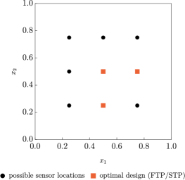
Figure 1: Left: The root-mean-square (R.M.S.) cubature errors of the FTP method (a) and STP method (b) applied to the PDE problem (9.1) subject to an affine and uniform representation of the input random field (i) corresponding to the optimal design. Right: The optimal design obtained using both approaches.

(a)

Figure 2: Left: The root-mean-square (R.M.S.) cubature errors of the FTP method (a) and STP method (b) applied to the PDE problem (9.1) subject to a periodic representation of the input random field (ii) corresponding to the optimal design. Right: The optimal design obtained using both approaches.

Remark 9.1

The conditions of Assumptions 7.1–8.1 are satisfied due to the truncation of the data domain (A2.1), the regularity analysis presented in Lemmata 5.3 and 5.7 (A2.2) and the mixed regularity analysis presented in Section 5.2 (A2.3).

In all experiments, we compute the value of the EIG for each ${\boldsymbol{\xi}}\in\Xi$ and as the optimal design, we choose the design ${\boldsymbol{\xi}}^{*}\in\Xi$ minimizing the value of the objective function corresponding to the largest number of cubature points for each experiment (a)–(c).

As the generating vector for both integrals in cases (a) and (b), as well as the inner integral in part (c), we used the off-the-shelf lattice rule (kuogeneratingvector, , lattice-32001-1024-1048576.3600). For each cubature node, the PDE was solved using a first-order finite element method with mesh width $h=2^{-5}$. The root-mean-square error was approximated with respect to $R=16$ random shifts for experiments (a) and (b), and the results these experiments subject to input random field (i) are given in Figure 1, while the corresponding results for the input random field (ii) are given in Figure 2.

The convergence rate subject to the full tensor product cubature scheme is close to $\mathcal{O}(N^{-1/2})$ while the convergence rates for the sparse tensor product cubature scheme are nearly $\mathcal{O}(N^{-1})$. The results computed using the periodic parameterization appear to have a slightly improved rate of decay compared to the affine and uniform parameterization.

The results for experiment (c) are given in Figure 3. We approximated the inner integral using a lattice rule with a single random shift and, instead of estimating the root-mean-square error, we obtained the absolute errors of the FTP and STP methods by computing the difference against reference solutions corresponding to $17\,989\,120$ nodes (FTP) and $468\,732$ nodes (STP).

Since both the inner and outer integral are now approximated by higher-order cubatures, the convergence rate subject to the full tensor product cubature scheme is close to $\mathcal{O}(N^{-1})$ while the sparse tensor product construction achieves a convergence order of roughly $\mathcal{O}(N^{-2})$. We note that the preasymptotic regimes are relatively long, so the linear fits were constructed using the last three data points for the FTP method and the last five data points for the STP method.

(a)

Figure 3: Left: The absolute errors of the FTP and STP methods using approach (c) applied to the PDE problem (9.1) subject to a periodic representation of the input random field (ii) corresponding to the optimal design. Right: The optimal design obtained using both approaches.

Remark 9.2

Alternatively, one could use any higher-order cubature method such as interlaced polynomial lattice rules (cf., e.g., spodpaper14 ) to approximate the inner or outer integrals. The regularity analysis developed in Section 5 can be adapted to construct tailored lattice rules for this class of quasi-Monte Carlo methods as well.

10 Conclusions

In summary, this paper represents a significant advancement in the field of BOED for problems governed by PDEs. By establishing parametric regularity, we have delved deeper into the nuances of the design problem, enriching our comprehension of its underlying dynamics. Moreover, our thorough error analysis of the full tensor QMC method has showcased its robustness and efficacy, with convergence rates remaining independent of parameter dimensions.

The introduction of the sparse tensor method has unveiled considerable potential, providing a promising avenue for enhancing convergence rates in nested integrals and recovering original rates. Through numerical verification of predicted convergence rates for a specific elliptic problem, we have furnished empirical validation to support our theoretical findings, affirming the practical feasibility of our proposed methodologies.

The analysis of the sparse tensor approach for nonlinear functions within the inner integral is particularly intriguing, offering avenues for exploration in other domains such as machine learning and statistics, where nested expectations are prevalent, such as variational autoencoders or probabilistic programming systems. Future research endeavors will focus on extending our findings to encompass a broader spectrum of forward problems, not limited to the elliptic model problem.

While our analysis has demonstrated the independence of convergence behavior on parameter dimensions under suitable assumptions, the dependence on data dimensions and noise covariance could be pivotal, especially in scenarios involving informative or sequential data collection processes. In forthcoming studies, we aim to explore techniques grounded in preconditioners to mitigate this effect, building upon prior works in the field DBLP:journals/nm/SchillingsSW20 .

Appendix A Technical results

The two summation identities appearing in the regularity analysis of Subsection 5.1 can be established using hypergeometric summation.

Lemma A.1

Let $v\geq 1$. Then

$$\sum_{\ell=1}^{v}\frac{1}{(v-\ell)!(\ell-1)!}=\frac{2^{v-1}}{(v-1)!}.$$

Proof

We prove this using Sister Celine’s method aeqb . We define $T(v):=\sum_{\ell=1}^{v}\frac{1}{(v-\ell)!(\ell-1)!}$ and $F(v,\ell):=\frac{1}{(v-\ell)!(\ell-1)!}$. Letting $a,b,c\in\mathbb{R}$ be undetermined coefficients, we first seek a non-trivial solution to

$$aF(v,\ell)+bF(v,\ell+1)+cF(v+1,\ell+1)=0.$$ (A.1)

Plugging in the values of $F$ into the above formula and regrouping the equation as a polynomial in terms of $\ell$ yields

$$(a-b)\ell+bv+c=0.$$

This yields $b=a$, and $c=-av$ for $a\in\mathbb{R}$. The relation (A.1) thus simplifies to

$$F(v,\ell)=vF(v+1,\ell+1)-F(v,\ell+1).$$

By taking the sum over $\ell\in\{1,\ldots,v\}$, we obtain

$$T(v)=vT(v+1)-T(v)-vF(v+1,1)+F(v,1)-F(v,v+1).$$

Noting that $F(v+1,1)=\frac{1}{v!}$, $F(v,1)=\frac{1}{(v-1)!}$, and $F(v,v+1)=0$ (by convention), we obtain the recurrence

$$T(v+1)=\frac{2}{v}T(v),\quad T(1)=1.$$

The claim is an immediate consequence of this recurrence relation.∎

Lemma A.2

Let $v\geq 1$ and $2\leq\lambda\leq v+1$. Then

$$\sum_{\ell=\lambda-1}^{v}(v-\ell+1)\frac{(\ell-1)!}{(\ell-\lambda+1)!}=\frac{(v+1)!}{(v-\lambda+1)!\lambda(\lambda-1)}.$$ (A.2)

Proof

We start by proving a different yet related identity:

$$\sum_{\ell=b}^{v}(a-\ell)\frac{(\ell-1)!}{(\ell-b)!}=\frac{(b-v-1)(bv+b-ab-a)v!}{b(1+b)(v-b+1)!}.$$ (A.3)

Let $t_{\ell}:=(a-\ell)\frac{(\ell-1)!}{(\ell-b)!}$. It turns out that the left-hand side expression in (A.3) is Gosper-summable: it is straightforward to check that $t_{\ell}=z_{\ell+1}-z_{\ell}$, where

$$z_{\ell}:=\frac{(a+ab-b\ell)(\ell-1)!}{b(1+b)(\ell-b-1)!}.$$

In consequence,

$$\sum_{\ell=b}^{v}(a-\ell)\frac{(\ell-1)!}{(\ell-b)!}=\sum_{\ell=b}^{v}t_{\ell}=z_{v+1}-z_{b}=\frac{(b-v-1)(bv+b-ab-a)v!}{b(1+b)(v-b+1)!},$$

as desired.

The equation (A.2) follows by substituting $a=v+1$ and $b=\lambda-1$ into (A.3).∎

Appendix B QMC analysis under periodic change of variables

We begin by proving a general result on the parametric regularity bounds for smooth Banach space valued functions under a periodic change of variables.

Theorem B.1

Let $X$ be a separable Banach space. Let $(\Gamma_{k})_{k\geq 0}$ and $\boldsymbol{b}=(b_{j})_{j\geq 1}$ be sequences of nonnegative numbers and $C_{0}>0$. Suppose that $u(\boldsymbol{\theta})\in X$ is infinitely many times continuously differentiable such that

$$\|\partial_{{\boldsymbol{\theta}}}^{{\boldsymbol{\nu}}}u({\boldsymbol{\theta}})\|_{X}\leq C_{0}\Gamma_{|{\boldsymbol{\nu}}|}{\boldsymbol{b}}^{{\boldsymbol{\nu}}}\quad\text{for all}~{}{\boldsymbol{\nu}}\in\mathbb{N}_{0}^{s}~{}\text{and}~{}{\boldsymbol{\theta}}\in\Theta_{s}:=[-1/2,1/2]^{s}.$$

Then the function defined by

$$u_{\rm per}({\boldsymbol{\theta}}):=u(\sin(2\pi{\boldsymbol{\theta}})),\quad{\boldsymbol{\theta}}\in\Theta_{s},$$ (B.1)

satisfies the regularity bound

$$\|\partial_{{\boldsymbol{\theta}}}^{\boldsymbol{\nu}}u_{\rm per}(\boldsymbol{\theta})\|_{X}\leq(2\pi)^{|{\boldsymbol{\nu}}|}C_{0}\sum_{\boldsymbol{m}\leq\boldsymbol{\nu}}\Gamma_{|\boldsymbol{m}|}\boldsymbol{b}^{\boldsymbol{m}}\prod_{j\geq 1}S(\nu_{j},m_{j})$$

for all $\boldsymbol{\nu}\in\mathbb{N}_{0}^{s}$ and $\boldsymbol{\theta}\in\Theta_{s}$, where $S(\cdot,\cdot)$ denotes the Stirling number of the second kind.

We begin by outlining the proof strategy. The composition (B.1) suggests using Faà di Bruno’s formula savits : for $\boldsymbol{\nu}\in\mathbb{N}_{0}^{s}\setminus\{\mathbf{0}\}$, there holds

$$\partial_{{\boldsymbol{\theta}}}^{\boldsymbol{\nu}}u_{\rm per}(\boldsymbol{\theta})=\sum_{\begin{subarray}{c}\boldsymbol{\lambda}\in\mathbb{N}_{0}^{s}\\ 1\leq|\boldsymbol{\lambda}|\leq|\boldsymbol{\nu}|\end{subarray}}\partial_{\boldsymbol{\theta^{\prime}}}^{\boldsymbol{\lambda}}u(\boldsymbol{\theta^{\prime}})\bigg{|}_{\boldsymbol{\theta^{\prime}}=\sin(2\pi\boldsymbol{\theta})}\kappa_{\boldsymbol{\nu},\boldsymbol{\lambda}}(\boldsymbol{\theta}),$$ (B.2)

where the sequence $(\kappa_{\boldsymbol{\nu},\boldsymbol{\lambda}}(\boldsymbol{\theta}))$ is defined recursively by

$$\kappa_{\boldsymbol{\nu},\mathbf{0}}\equiv\delta_{\boldsymbol{\nu},\mathbf{0}},$$

$$\kappa_{\boldsymbol{\nu},\boldsymbol{\lambda}}\equiv 0\quad\text{if}~{}|\boldsymbol{\nu}|<|\boldsymbol{\lambda}|~{}\text{or}~{}\boldsymbol{\lambda}\not\geq\mathbf{0},$$

$$\kappa_{\boldsymbol{\nu}+\boldsymbol{e}_{j},\boldsymbol{\lambda}}(\boldsymbol{\theta})=\sum_{\ell\in{\rm supp}(\boldsymbol{\lambda})}\sum_{\boldsymbol{m}\leq\boldsymbol{\nu}}\binom{\boldsymbol{\nu}}{\boldsymbol{m}}\partial_{{\boldsymbol{\theta}}}^{\boldsymbol{m}+\boldsymbol{e}_{j}}\sin(2\pi\theta_{\ell})\kappa_{\boldsymbol{\nu}-\boldsymbol{m},\boldsymbol{\lambda}-\boldsymbol{e}_{\ell}}(\boldsymbol{\theta})$$

$$=\sum_{m_{j}=0}^{\nu_{j}}\binom{\nu_{j}}{m_{j}}\partial_{\theta_{j}}^{m_{j}+1}\sin(2\pi\theta_{j})\kappa_{\boldsymbol{\nu}-m_{j}\boldsymbol{e}_{j},\boldsymbol{\lambda}-\boldsymbol{e}_{j}}(\boldsymbol{\theta})\quad\text{otherwise}.$$

Making use of the fact that

$$\bigg{|}\frac{{\rm d}^{k}}{{\rm d}\theta^{k}}\sin(2\pi\theta)\bigg{|}=\bigg{|}(2\pi)^{k}\sin\bigg{(}2\pi\theta+k\,\frac{\pi}{2}\bigg{)}\bigg{|}\leq(2\pi)^{k},$$

we can find an upper bound for the sequence $(\kappa_{\boldsymbol{\nu},\boldsymbol{\lambda}}(\boldsymbol{\theta}))$ defined by an auxiliary sequence $(\beta_{\boldsymbol{\nu},\boldsymbol{\lambda}})$ given by the recursion

$$\beta_{\boldsymbol{\nu},\mathbf{0}}=\delta_{\boldsymbol{\nu},\mathbf{0}},$$

$$\beta_{\boldsymbol{\nu},\boldsymbol{\lambda}}=0\quad\text{if}~{}|\boldsymbol{\nu}|<|\boldsymbol{\lambda}|~{}\text{or}~{}\boldsymbol{\lambda}\not\geq\mathbf{0},$$

$$\beta_{\boldsymbol{\nu}+\boldsymbol{e}_{j},\boldsymbol{\lambda}}=\sum_{m_{j}=0}^{\nu_{j}}\binom{\nu_{j}}{m_{j}}(2\pi)^{m_{j}+1}\beta_{\boldsymbol{\nu}-m_{j}\boldsymbol{e}_{j},\boldsymbol{\lambda}-\boldsymbol{e}_{j}}\quad\text{otherwise.}$$

This sequence has the following closed form solution.

Lemma B.2

There holds

$$\beta_{\boldsymbol{\nu},\boldsymbol{\lambda}}=(2\pi)^{|\boldsymbol{\nu}|}\prod_{j\geq 1}S(\nu_{j},\lambda_{j})\quad\text{for all}~{}\boldsymbol{\nu},\boldsymbol{\lambda}\in\mathbb{N}_{0}^{s}.$$

Proof

Let $\boldsymbol{\lambda}\in\mathbb{N}_{0}^{s}$ be arbitrary. The proof is carried out by induction with respect to the modulus of $\boldsymbol{\nu}\in\mathbb{N}_{0}^{s}$. The base step is resolved by observing that

$$\beta_{\mathbf{0},\mathbf{0}}=1=\prod_{j\geq 1}S(0,0),$$

and, if $\boldsymbol{\lambda}\neq\mathbf{0}$,

$$\beta_{\mathbf{0},\boldsymbol{\lambda}}=0=\prod_{j\geq 1}S(0,\lambda_{j}),$$

where the second inequality holds due to ${\rm supp}(\boldsymbol{\lambda})\neq\varnothing$.

To resolve the induction step, let $\boldsymbol{\nu}\in\mathbb{N}_{0}^{s}$ and suppose that the claim has already been proved for all multi-indices with modulus less than or equal to $|\boldsymbol{\nu}|$. Let $j\geq 1$ be arbitrary. Then

$$\beta_{\boldsymbol{\nu}+\boldsymbol{e}_{j},\boldsymbol{\lambda}} =\sum_{m_{j}=0}^{\nu_{j}}\binom{\nu_{j}}{m_{j}}(2\pi)^{m_{j}+1}(2\pi)^{|\boldsymbol{\nu}|-m_{j}}S(\nu_{j}-m_{j},\lambda_{j}-1)\prod_{i\neq j}S(\nu_{i},\lambda_{i})$$

$$=(2\pi)^{|\boldsymbol{\nu}|+1}\prod_{i\neq j}S(\nu_{i},\lambda_{i})\sum_{m_{j}=0}^{\nu_{j}}\binom{\nu_{j}}{m_{j}}S(\nu_{j}-m_{j},\lambda_{j}-1)$$

$$=(2\pi)^{|\boldsymbol{\nu}|+1}\bigg{(}\prod_{i\neq j}S(\nu_{i},\lambda_{i})\bigg{)}S(\nu_{j}+1,\lambda_{j}),$$

where the final equality is an immediate consequence of (nist, , formula 26.8.23).∎

Proof (Proof of Theorem B.1)

Since $\kappa_{\boldsymbol{\nu},\boldsymbol{\lambda}}\leq\beta_{\boldsymbol{\nu},\boldsymbol{\lambda}}$ holds by construction, we may plug into (B.2) the identity proved in Lemma B.2 and use the bound (A2) to obtain

$$\|\partial_{{\boldsymbol{\theta}}}^{\boldsymbol{\nu}}u_{\rm per}(\boldsymbol{\theta})\|_{X} \leq(2\pi)^{|\boldsymbol{\nu}|}C_{0}\sum_{\begin{subarray}{c}\boldsymbol{\lambda}\in\mathbb{N}_{0}^{s}\\ 1\leq|\boldsymbol{\lambda}|\leq|\boldsymbol{\nu}|\end{subarray}}\Gamma_{|\boldsymbol{\lambda}|}\boldsymbol{b}^{\boldsymbol{\lambda}}\prod_{j\geq 1}S(\nu_{j},\lambda_{j})$$

$$=(2\pi)^{|\boldsymbol{\nu}|}C_{0}\sum_{\boldsymbol{\lambda}\leq\boldsymbol{\nu}}\Gamma_{|\boldsymbol{\lambda}|}\boldsymbol{b}^{\boldsymbol{\lambda}}\prod_{j\geq 1}S(\nu_{j},\lambda_{j})$$

since $\prod_{j\geq 1}S(\nu_{j},\lambda_{j})=0$ whenever $\boldsymbol{\lambda}\not\leq\boldsymbol{\nu}$.∎

Remark B.3

The Faà di Bruno formula in was developed for scalar-valued functions in savits , but we applied it above for Banach space valued functions. This is not an issue as can be seen by the following simple argument: for arbitrary $G\in X^{\prime}$, there holds

$$\langle G,\partial_{{\boldsymbol{\theta}}}^{{\boldsymbol{\nu}}}u_{\rm per}({\boldsymbol{\theta}})\rangle_{X^{\prime},X} =\partial_{{\boldsymbol{\theta}}}^{{\boldsymbol{\nu}}}\langle G,u_{\rm per}({\boldsymbol{\theta}})\rangle_{X^{\prime},X}$$

$$=\partial_{{\boldsymbol{\theta}}}^{{\boldsymbol{\nu}}}(\langle G,u(\cdot)\rangle_{X^{\prime},X}\circ\sin(2\pi{\boldsymbol{\theta}}))$$

$$=\sum_{\begin{subarray}{c}\boldsymbol{\lambda}\in\mathbb{N}_{0}^{s}\\ 1\leq|\boldsymbol{\lambda}|\leq|{\boldsymbol{\nu}}|\end{subarray}}\partial_{\boldsymbol{\theta^{\prime}}}^{\boldsymbol{\lambda}}\langle G,u(\boldsymbol{\theta^{\prime}})\rangle_{X^{\prime},X}\bigg{|}_{\boldsymbol{\boldsymbol{\theta}^{\prime}}=\sin(2\pi{\boldsymbol{\theta}})}\kappa_{{\boldsymbol{\nu}},\boldsymbol{\lambda}}({\boldsymbol{\theta}})$$

$$=\bigg{\langle}G,\sum_{\begin{subarray}{c}\boldsymbol{\lambda}\in\mathbb{N}_{0}^{s}\\ 1\leq|\boldsymbol{\lambda}|\leq|{\boldsymbol{\nu}}|\end{subarray}}\partial_{\boldsymbol{\theta^{\prime}}}^{\boldsymbol{\lambda}}u(\boldsymbol{\theta^{\prime}})\bigg{|}_{\boldsymbol{\theta^{\prime}}=\sin(2\pi{\boldsymbol{\theta}})}\kappa_{{\boldsymbol{\nu}},\boldsymbol{\lambda}}({\boldsymbol{\theta}})\bigg{\rangle}_{X^{\prime},X},$$

where the scalars $(\kappa_{{\boldsymbol{\nu}},\boldsymbol{\lambda}}({\boldsymbol{\theta}}))$ are defined using exactly the same recursion as before. Since the above derivation holds for all $G\in X^{\prime}$, we conclude that Faà di Bruno’s formula (B.2) is valid for Banach space valued functions.

The significance of the preceding result can be understood as follows: in order to obtain the parametric regularity bound for a given problem under the periodic paradigm, it is in principle sufficient to carry out the parametric regularity analysis under the assumption of an underlying affine and uniform random field and then apply Theorem B.1 to obtain the corresponding regularity bound for the periodically transformed problem.

As a corollary, we obtain the following analogues of Lemmata 5.3 and 5.6 for the periodic model problem (4.3).

Lemma B.4

Let ${\boldsymbol{\nu}}\in\mathbb{N}_{0}^{s}\setminus\{\mathbf{0}\}$. Then under assumptions (A1.1)–(A1.3), there holds for (4.3) that

$$|\partial_{\boldsymbol{\theta}}^{\boldsymbol{\nu}}{\rm e}^{-\frac{1}{2}\|\boldsymbol{y}-G_{s,{\rm per}}(\boldsymbol{\theta},\boldsymbol{\xi})\|_{\Gamma^{-1}}^{2}}|$$

$$\leq 3.82^{k}(2\pi)^{|{\boldsymbol{\nu}}|}\sum_{\boldsymbol{m}\leq{\boldsymbol{\nu}}}C^{|\boldsymbol{m}|}2^{|\boldsymbol{m}|-1}\mu_{\min}^{-|\boldsymbol{m}|/2}|\boldsymbol{m}|!\boldsymbol{b}^{\boldsymbol{m}}\prod_{j\geq 1}S(\nu_{j},m_{j})$$

for all ${\boldsymbol{\theta}}\in\Theta_{s}$, ${\boldsymbol{y}}\in[-K,K]^{k}$, and ${\boldsymbol{\xi}}\in\Xi$.

Lemma B.5

Let ${\boldsymbol{\nu}}\in\mathbb{N}_{0}^{s}\setminus\{\mathbf{0}\}$ and ${\boldsymbol{\eta}}\in\mathbb{N}_{0}^{k}\setminus\{\mathbf{0}\}$. Then under assumptions (A1.1)–(A1.3), there holds for (4.3) that

$$|\partial_{{\boldsymbol{y}}}^{{\boldsymbol{\eta}}}\partial_{{\boldsymbol{\theta}}}^{{\boldsymbol{\nu}}}{\rm e}^{-\frac{1}{2}\|{\boldsymbol{y}}-G_{s,{\rm per}}({\boldsymbol{\theta}},{\boldsymbol{\xi}})\|_{\Gamma^{-1}}^{2}}|$$

$$\leq\frac{1}{2}\cdot 2.2^{k}k{\rm e}^{2k}{\boldsymbol{\eta}}!(2\pi)^{|{\boldsymbol{\nu}}|}\sum_{\boldsymbol{m}\leq{\boldsymbol{\nu}}}(4C)^{|\boldsymbol{m}|}\mu_{\min}^{-|\boldsymbol{m}|-1/2}R^{|\boldsymbol{m}|}|\boldsymbol{m}|!{\boldsymbol{b}}^{\boldsymbol{m}}\prod_{j\geq 1}S(\nu_{j},m_{j})$$

for all ${\boldsymbol{\theta}}\in\Theta_{s}$, ${\boldsymbol{y}}\in[-K,K]^{k}$, and ${\boldsymbol{\xi}}\in\Xi$.

Let $F\in C([0,1)^{s})$ be a smooth, 1-periodic function with dominating mixed smoothness of order $\alpha>1$ and consider the cubature rule

$$Q_{s,n}(F):=\frac{1}{n}\sum_{i=1}^{n}F({\boldsymbol{t}}_{i})\approx\int_{[0,1]^{s}}F({\boldsymbol{\theta}})\,{\rm d}{\boldsymbol{\theta}}=:I_{s}(F)$$

over (unshifted) lattice points (3.1). By defining the norm

$$\|F\|_{\mathcal{K}_{s,\alpha,{\boldsymbol{\gamma}}}}:=\sup_{\boldsymbol{h}\in\mathbb{Z}^{s}}|\widehat{F}(\boldsymbol{h})|r_{\alpha}(\boldsymbol{\gamma},\boldsymbol{h}),\quad r_{\alpha}({\boldsymbol{\gamma}},\boldsymbol{h}):=\gamma_{{\rm supp}(\boldsymbol{h})}^{-1}\prod_{j\in{\rm supp}(\boldsymbol{h})}|h_{j}|^{\alpha},$$

where ${\rm supp}(\boldsymbol{h}):=\{j\in\{1:s\}:h_{j}\neq 0\}$ and $\widehat{F}(\boldsymbol{h}):=\int_{[0,1]^{s}}F({\boldsymbol{\theta}}){\rm e}^{-2\pi{\rm i}{\boldsymbol{\theta}}\cdot\boldsymbol{h}}\,{\rm d}{\boldsymbol{\theta}}$ for $\boldsymbol{h}\in\mathbb{Z}^{s}$, and ${\boldsymbol{\gamma}}=(\gamma_{\mathrm{\mathfrak{u}}})_{\mathrm{\mathfrak{u}}\subseteq\{1:s\}}$ denotes a collection of positive weights, we have the following.

Lemma B.6 (cf. korobovpaper )

Let $s\in\mathbb{N}$, $\alpha>1$, and let ${\boldsymbol{\gamma}}=(\gamma_{\mathrm{\mathfrak{u}}})_{\mathrm{\mathfrak{u}}\subseteq\{1:s\}}$ be a collection of positive weights. Let $F\in C([0,1)^{s})$ be a 1-periodic function with respect to each of its variables such that $\|F\|_{\mathcal{K}_{s,\alpha,{\boldsymbol{\gamma}}}}<\infty$. An $s$-dimensional lattice rule with $n=2^{m}$ points, $m\geq 0$, can be constructed by a CBC algorithm such that, for all $\lambda\in(1/\alpha,1]$,

$$|I_{s}(F)-Q_{s,n}(F)|\leq\bigg{(}\frac{2}{n}\sum_{\varnothing\neq\mathfrak{u}\subseteq\{1:s\}}\gamma_{\mathfrak{u}}^{\lambda}(2\zeta(\alpha\lambda))^{|\mathrm{\mathfrak{u}}|}\bigg{)}^{1/\lambda}\|F\|_{\mathcal{K}_{s,\alpha,\boldsymbol{\gamma}}},$$

where $\zeta(x):=\sum_{\ell=1}^{\infty}\ell^{-x}$ is the Riemann zeta function for $x>1$.

When $\alpha\geq 2$ is an integer, there holds

$$\|F\|_{\mathcal{K}_{s,\alpha,{\boldsymbol{\gamma}}}}\leq\max_{\mathrm{\mathfrak{u}}\subseteq\{1:s\}}\frac{1}{(2\pi)^{\alpha|\mathrm{\mathfrak{u}}|}}\frac{1}{\gamma_{\mathrm{\mathfrak{u}}}}\int_{[0,1]^{|\mathrm{\mathfrak{u}}|}}\bigg{|}\int_{[0,1]^{s-|\mathrm{\mathfrak{u}}|}}\bigg{(}\prod_{j\in\mathrm{\mathfrak{u}}}\frac{\partial^{\alpha}}{\partial y_{j}^{\alpha}}\bigg{)}F({\boldsymbol{y}})\,{\rm d}{\boldsymbol{y}}_{-\mathrm{\mathfrak{u}}}\bigg{|}\,{\rm d}{\boldsymbol{y}}_{\mathrm{\mathfrak{u}}}$$

provided that $F$ has mixed partial derivatives of order $\alpha$.

We consider the parametric regularity of the inner integrand appearing in the expression

$$\int_{\Theta_{s}}f_{\rm per}({\boldsymbol{\theta}},{\boldsymbol{y}})\,{\rm d}{\boldsymbol{\theta}},\quad f_{\rm per}({\boldsymbol{\theta}},{\boldsymbol{y}}):=C_{k,\Gamma}{\rm e}^{-\frac{1}{2}\|{\boldsymbol{y}}-G_{s,{\rm per}}({\boldsymbol{\theta}},{\boldsymbol{\xi}})\|_{\Gamma^{-1}}^{2}}.$$ (B.3)

In complete analogy to the derivation in KKS , we obtain the following result.

Theorem B.7

Let $n=2^{m}$, $m\geq 0$. Then under assumptions (A1.1)–(A1.3), it is possible to use a CBC algorithm to obtain a generating vector $\boldsymbol{z}\in\mathbb{N}^{s}$ such that the rank-1 lattice rule for the integrand $f_{\rm per}$ of (B.3) satisfies the root-mean-square error estimate

$$|I_{s}(f_{\rm per})-{Q}_{s,n}(f_{\rm per})|\leq Cn^{-1/p},$$

where the constant $C>0$ is independent of the dimension $s$, provided that the smoothness-driven product and order dependent (SPOD) weights

$$\gamma_{\mathrm{\mathfrak{u}}}:=\sum_{\boldsymbol{m}_{\mathrm{\mathfrak{u}}}\in\{1:\alpha\}^{|\mathrm{\mathfrak{u}}|}}C^{|\boldsymbol{m}_{\mathrm{\mathfrak{u}}}|}2^{|\boldsymbol{m}_{\mathrm{\mathfrak{u}}}|-1}\mu_{\min}^{-|\boldsymbol{m}_{\mathrm{\mathfrak{u}}}|/2}|\boldsymbol{m}_{\mathrm{\mathfrak{u}}}|!\prod_{j\in\mathrm{\mathfrak{u}}}\big{(}b_{j}^{m_{j}}S(\alpha,m_{j})\big{)}$$

are used as inputs to the CBC algorithm with $\alpha=\lfloor 1/p\rfloor+1$.

The convergence rates for the full tensor product and sparse tensor product approximations of the double integral subject to the periodically parameterized forward model, i.e.,

$$\int_{[-K,K]^{k}}g\bigg{(}\int_{\Theta_{s}}f_{\rm per}({\boldsymbol{\theta}},{\boldsymbol{y}})\,{\rm d}{\boldsymbol{\theta}}\bigg{)}\,{\rm d}{\boldsymbol{y}},\quad g(y)=x\log x,$$

coincide with those presented in Theorems 7.3 and 8.3 when the outer integral is discretized using a first-order method. However, if the outer integral is approximated using a higher-order cubature method—such that its rate is balanced with the higher-order rate exhibited by the periodically parameterized inner integral—then the statements of Theorems 7.3 and 8.3 hold true with the obvious substitution of higher-order convergence rates in place of the first-order rates. In particular, the dimension independence can be established. Furthermore, the sparse tensor product can recover the optimal rate up to a logarithmic factor. We demonstrate these effects in the numerical experiments of Section 9.

References

• (1) Abramowitz, M., Stegun, I.A.: Handbook of Mathematical Functions With Formulas, Graphs, and Mathematical Tables, National Bureau of Standards Applied Mathematics Series, vol. 55. For sale by the Superintendent of Documents, U.S. Government Printing Office, Washington, D.C. (1964)
• (2) Alexanderian, A.: Optimal experimental design for infinite-dimensional Bayesian inverse problems governed by PDEs: a review. Inverse Problems 37(4), 043 ​001 (2021). DOI 10.1088/1361-6420/abe10c
• (3) Alexanderian, A., Petra, N., Stadler, G., Ghattas, O.: A-optimal design of experiments for infinite dimensional Bayesian linear inverse problems with regularized $l_{\infty}$-sparsification. SIAM J. Sci. Comput. 36(5), A2122–A2148 (2014). DOI 10.1137/130933381
• (4) Atkinson, A., Donev, A., Tobias, R.: Optimum experimental designs, with SAS, vol. 34. Oxford University Press (2007). DOI 10.1111/j.1751-5823.2007.00030˙5.x
• (5) Bartuska, A., Carlon, A.G., Espath, L., Krumscheid, S., Tempone, R.: Double-loop randomized quasi-Monte Carlo estimator for nested integration. Preprint arXiv:2302.14119 [math.NA] (2024)
• (6) Beck, J., Dia, B.M., Espath, L.F., Long, Q., Tempone, R.: Fast Bayesian experimental design: Laplace-based importance sampling for the expected information gain. Comput. Methods Appl. Mech. Engrg. 334, 523–553 (2018). DOI 10.1016/j.cma.2018.01.053
• (7) Beck, J., Tempone, R., Nobile, F., Tamellini, L.: On the optimal polynomial approximation of stochastic PDEs by Galerkin and collocation methods. Maths. Models Methods Appl. Sci. 22(9), 125 ​0023 (2012). DOI 10.1142/S0218202512500236
• (8) Belkhir, A.: The multivariate Lah and Stirling numbers. J. Integer Seq. 23, 20.4.5 (2020)
• (9) Chaloner, K., Verdinelli, I.: Bayesian experimental design: a review. Statist. Sci. 10(3), 273–304 (1995). DOI 10.1214/ss/1177009939
• (10) Cohen, A., DeVore, R., Schwab, C.: Convergence rates of best $N$-term Galerkin approximations for a class of elliptic sPDEs. Found. Comput. Math. 10, 615–646 (2010). DOI 10.1007/s10208-010-9072-2
• (11) Cools, R., Kuo, F.Y., Nuyens, D.: Constructing embedded lattice rules for multivariate integration. SIAM J. Sci. Comput. 28, 2162–2188 (2006). DOI 10.1137/06065074X
• (12) Dick, J., Kuo, F.Y., Le Gia, Q.T., Nuyens, D., Schwab, C.: Higher order QMC Petrov–Galerkin discretization for affine parametric operator equations with random field inputs. SIAM J. Numer. Anal. 52(6), 2676–2702 (2014). DOI 10.1137/13094398
• (13) Dick, J., Kuo, F.Y., Sloan, I.H.: High-dimensional integration: the quasi-Monte Carlo way. Acta Numer. 22, 133–288 (2013). DOI 10.1017/S0962492913000044
• (14) Dick, J., Sloan, I.H., Wang, X., Woźniakowski, H.: Good lattice rules in weighted Korobov spaces with general weights. Numer. Math. 103, 63–97 (2006). DOI 10.1007/s00211-005-0674-6
• (15) Gantner, R.N., Herrmann, L., Schwab, C.: Quasi–Monte Carlo integration for affine-parametric, elliptic PDEs: local supports and product weights. SIAM J. Numer. Anal. 56(1), 111–135 (2018). DOI 10.1137/16M1082597
• (16) Gilbert, A.D., Graham, I.G., Kuo, F.Y., Scheichl, R., Sloan, I.H.: Analysis of quasi-Monte Carlo methods for elliptic eigenvalue problems with stochastic coefficients. Numer. Math. 142(4), 863–915 (2019). DOI 10.1007/s00211-019-01046-6
• (17) Gilbert, A.D., Scheichl, R.: Multilevel quasi-Monte Carlo for random elliptic eigenvalue problems I: regularity and error analysis. IMA J. Numer. Anal. 44(1), drad011 (2023). DOI 10.1093/imanum/drad011
• (18) Gilch, A., Griebel, M., Oettershagen, J.: Sparse tensor product approximation for a class of generalized method of moments estimators. Int. J. Uncertain. Quantif. 12(2), 53–79 (2022). DOI 10.1615/Int.J.UncertaintyQuantification.2021037549
• (19) Guth, P.A., Kaarnioja, V.: Generalized dimension truncation error analysis for high-dimensional numerical integration: lognormal setting and beyond. SIAM J. Numer. Anal. 62(2), 872–892 (2024). DOI 10.1137/23M1593188
• (20) Guth, P.A., Kaarnioja, V., Kuo, F.Y., Schillings, C., Sloan, I.H.: A quasi-Monte Carlo method for optimal control under uncertainty. SIAM/ASA J. Uncertain. Quantif. 9(2), 354–383 (2021). DOI 10.1137/19M1294952
• (21) Guth, P.A., Kaarnioja, V., Kuo, F.Y., Schillings, C., Sloan, I.H.: Parabolic PDE-constrained optimal control under uncertainty with entropic risk measure using quasi-Monte Carlo integration. Numer. Math., 156, 565–608 (2024). DOI 10.1007/s00211-024-01397-9
• (22) Guth, P.A., Schillings, C., Weissmann, S.: One-shot learning of surrogates in PDE-constrained optimization under uncertainty. Preprint arXiv:2112.11126 [math.OC] (2021)
• (23) Guth, P.A., Van Barel, A.: Multilevel quasi-Monte Carlo for optimization under uncertainty. Numer. Math. 154, 443–484 (2023). DOI 10.1007/s00211-023-01364-w
• (24) Harbrecht, H., Peters, M., Siebenmorgen, M.: On the quasi-Monte Carlo method with Halton points for elliptic PDEs with log-normal diffusion. Math. Comp. 86, 771–797 (2017). DOI 10.1090/mcom/3107
• (25) Herrmann, L., Keller, M., Schwab, C.: Quasi-Monte Carlo Bayesian estimation under Besov priors in elliptic inverse problems. Math. Comp. 90, 1831–1860 (2021). DOI 10.1090/mcom/3615
• (26) Huan, X., Marzouk, Y.M.: Simulation-based optimal Bayesian experimental design for nonlinear systems. J. Comput. Phys. 232(1), 288–317 (2013). DOI 10.1016/j.jcp.2012.08.013
• (27) Kaarnioja, V., Kuo, F.Y., Sloan, I.H.: Uncertainty quantification using periodic random variables. SIAM J. Numer. Anal. 58(2), 1068–1091 (2020). DOI 10.1137/19M1262796
• (28) Koval, K., Herzog, R., Scheichl, R.: Tractable optimal experimental design using transport maps. Preprint arXiv:2401.07971 [stat.CO] (2024)
• (29) Kuo, F.Y.: Lattice rule generating vectors.
https://web.maths.unsw.edu.au/~fkuo/lattice/
• (30) Kuo, F.Y., Nuyens, D.: Application of quasi-Monte Carlo methods to elliptic PDEs with random diffusion coefficients: a survey of analysis and implementation. Found. Comput. Math. 16, 1631–1696 (2016). DOI 10.1007/s10208-016-9329-5
• (31) Kuo, F.Y., Scheichl, R., Schwab, C., Sloan, I.H., Ullmann, E.: Multilevel quasi-Monte Carlo methods for lognormal diffusion problems. Math. Comp. 86, 2827–2860 (2017). DOI 10.1090/mcom/3207
• (32) Kuo, F.Y., Schwab, C., Sloan, I.H.: Quasi-Monte Carlo finite element methods for a class of elliptic partial differential equations with random coefficients. SIAM J. Numer. Anal. 50(6), 3351–3374 (2012). DOI 10.1137/110845537
• (33) Nuyens, D., Cools, R.: Fast algorithms for component-by-component construction of rank-1 lattice rules in shift-invariant reproducing kernel Hilbert spaces. Math. Comp. 75, 903–920 (2006). DOI 10.1090/s0025-5718-06-01785-6
• (34) Olver, F.W.J., Olde Daalhuis, A.B., Lozier, D.W., Schneider, B.I., Boisvert, R.F., Clark, C.W., Miller, B.R., Saunders, B.V., Cohl, H.S., McClain, M.A., eds.: NIST Digital Library of Mathematical Functions (2022). Release 1.1.6 of 2022-06-30, http://dlmf.nist.gov/
• (35) Pázman, A.: Foundations of Optimum Experimental Design. Springer Netherlands (1986)
• (36) Petkovšek, M., Wilf, H.S., Zeilberger, D.: $A=B$. CRC Press (1996)
• (37) Rainforth, T., Cornish, R., Yang, H., Warrington, A.: On nesting Monte Carlo estimators. In: J.G. Dy, A. Krause (eds.) Proceedings of the 35th International Conference on Machine Learning, ICML 2018, Stockholmsmässan, Stockholm, Sweden, July 10-15, 2018, Proceedings of Machine Learning Research, vol. 80, pp. 4264–4273. PMLR (2018)
• (38) Savits, T.H.: Some statistical applications of Faa di Bruno. J. Multivariate Anal. 97(10), 2131–2140 (2006). DOI 10.1016/j.jmva.2006.03.001
• (39) Schillings, C., Sprungk, B., Wacker, P.: On the convergence of the Laplace approximation and noise-level-robustness of Laplace-based Monte Carlo methods for Bayesian inverse problems. Numer. Math. 145(4), 915–971 (2020). DOI 10.1007/S00211-020-01131-1
• (40) Stuart, A.M.: Inverse problems: a Bayesian perspective. Acta Numer. 19, 451–559 (2010). DOI 10.1017/S0962492910000061
• (41) Ucinski, D.: Optimal Measurement Methods for Distributed Parameter System Identification, vol. 1. CRC press (2004). DOI 10.1201/9780203026786
• (42) Wu, K., O’Leary-Roseberry, T., Chen, P., Ghattas, O.: Large-scale Bayesian optimal experimental design with derivative-informed projected neural network. J. Sci. Comput. 95, 30 (2023). DOI 10.1007/s10915-023-02145-1