New physics as a possible explanation for the Amaterasu particle

Abstract

The Telescope Array experiment has recently reported the most energetic event detected in the hybrid technique era, with a reconstructed energy of 240 EeV, which has been named “Amaterasu” after the Shinto deity. Its origin is intriguing since no powerful enough candidate sources are located within the region consistent with its propagation horizon and arrival direction. In this work, we investigate the possibility of describing its origin in a scenario of new physics, specifically under a Lorentz Invariance Violation (LIV) assumption. The kinematics of UHECR propagation under a phenomenological LIV approach is investigated. The total mean free path for a particle with Amaterasu’s energy increases from a few Mpc to hundreds of Mpc for $-\delta_{\rm{had},0}>10^{-22}$, expanding significantly the region from which it could have originated. A combined fit of the spectrum and composition data of Telescope Array under different LIV assumptions was performed. The data is best fitted with some level of LIV both with and without Amaterasu. The improvement of the LIV fit is larger when Amaterasu is considered. New physics in the form of LIV could, thus, provide a plausible explanation for the Amaterasu particle.

1 Introduction

Ultra-high-energy cosmic rays (UHECR, $E>10^{18}$ eV) are the most energetic particles known in the Universe, forming the high-energy end of the energy spectrum of detected astroparticles. Due to their charged nature, which leads to deviations during the propagation in the presence of magnetic fields, their origins remain an open puzzle. Recently, an extra piece was added to this puzzle with the report of Telescope Array’s detection of an UHECR air shower with a reconstructed energy of $(244\pm 29,\rm{(stat.)}^{+51}_{-76}\,\rm{(syst.)})$ EeV (about 40 Joules) and reconstructed direction pointing to $(255.9\pm 0.6,\,16.1\pm 0.5)^{\circ}$ in equatorial coordinates [1].

This unique event was named Amaterasu after the Shinto goddess of the sun and represents the second-highest nominal energy ever detected (and highest in the hybrid detection technique era), only after the famous “Oh-My-God” particle detected with $(320\pm 0.9)$ EeV by the Fly Eye’s experiment in 1991 [2]. Moreover, its arrival direction is intriguing. UHECR with such energy are expected to quickly lose energy due to interactions with background photons, leading to a propagation horizon of a few tens of Mpc [3]. At the same time, at these energies, the magnetic field deviations are expected to be of the order of $20^{\circ}$ in the worst-case scenario [4]. With that, the origin point of Amaterasu could be restricted to a relatively small portion of the sky. Nevertheless, Amatarasu’s direction points to the Local Void, a region of the sky with a relatively small number of galaxies  [5]. [4] have further investigated it with the most up-to-date models for Galactic magnetic fields [6, 7, 8], finding no powerful enough candidate sources.

Alongside astrophysics explanations, such as a transient event or stronger magnetic fields, new physics could lead to scenarios in which Amaterasu can be described, in particular Lorentz Invariance Violation (LIV). The breaking of Lorentz symmetry has either been proposed or accommodated by several beyond the Standard Model theories [9]. The effects of LIV are expected to be suppressed up to the highest energies and, thus, astroparticles, in particular UHECR, have been extensively explored as important tools for testing such theories in a phenomenological approach [10, 11, 12, 13, 14, 15].

In this work, we investigate the possibility of describing Amaterasu under a scenario with Lorentz Invariance Violation. In section 2, we describe the considered LIV framework as well as the corresponding effects on the propagation of UHECR. In section 3, we present a combined fit for the data of Telescope Array under different LIV scenarios and how this is affected by Amaterasu. Finally, section 4 discusses this work’s conclusions and final remarks.

2 Lorentz Invariance Violation

2.1 Framework

The most commonly used LIV framework in phenomenological studies reduces the main effects to a shift in the energy dispersion relation [16, 17],

$$E^{2}_{a}=p^{2}_{a}+m^{2}_{a}+\sum_{n}\delta_{a,n}E^{n+2},$$ (2.1)

where $E$, $p$ and $m$ denote the particle’s energy, momentum, and mass, respectively. The particle species is denoted by $a$, given that LIV effects could in principle be independent for each particle type. The LIV effects of each order, $n$, are modulated by the LIV coefficient $\delta_{a,n}$, which can be either positive or negative. The most common approach is to investigate each LIV sector and order independently, i.e., to consider $\delta_{a,n}\neq 0$ for only a given $(a,n)$.

In this work, we use a similar approach to that used by the Pierre Auger Collaboration in their search for LIV imprints on their data [15]. We consider LIV only in the hadronic sector and investigate only the leading order ($\delta_{\rm{had},0}\neq 0$). As in [11] and [15], the LIV coefficients of protons, nuclei and pions relate via

$$\delta_{\rm{had},0}\coloneqq\delta_{p,0}=\frac{\delta_{\pi,0}}{2}=A^{n}\delta_{N,0}.$$ (2.2)

2.2 Propagation effects

UHECR propagation is limited by interactions with background photons. At the highest energies, two main interactions are dominant. Pion and heavier nuclei lose energy due to photopion production ($p+\gamma\rightarrow p+\pi$) and nuclei undergo photodisintegration, emitting one or two nucleons and becoming a lighter nucleus, (${}^{A}N+\gamma\rightarrow^{A-1}N+p/n$). These interactions govern the observables on Earth, strongly changing what was accelerated at the sources. Both interactions are strongly energy dependent, becoming effective above a few tens of EeV. With that, an energy-dependent propagation horizon is created, leading to an effective spectral index on Earth which differs from that accelerated at the sources. The photodisintegration acts on changing the particle species, creating a larger number of lighter and lower energy UHECR from a single higher energy heavy UHECR. This strongly influences both the spectrum and composition measured on Earth [3].

A change in the energy dispersion such as the one proposed in eq. 2.1 would impact the kinematics of these interactions [11, 18, 10]. In this work, we use the calculations for the LIV kinematics proposed by [18] and [10]. The main effect for $\delta_{\rm{had},0}<0$ is a reduction of the allowed four-momentum phase space of the particles, leading to a reduction in the number of interactions and, thus, an increase in the mean free path of propagating UHECR. This is illustrated in Fig. 1, which shows the mean free path for both interactions under different LIV scenarios. The mean free path diverges from the LI case above a given energy, which is modulated by the absolute value of $\delta_{\rm{had},0}$.

The total mean free path is particle dependent and, for nuclei, a sum of both effects. Fig. 2 shows how the total mean free path for a particle with Amaterasu’s energy changes as a function of the LIV coefficient for the two bracketing hypotheses, i.e., a proton or an iron primary. A LIV coefficient of $-\delta_{\rm{had},0}>10^{-22}$ is large enough to introduce a significant effect, increasing the mean free path up to three orders of magnitude for $\delta_{\rm{had},0}=-10^{-20}$. In those LIV scenarios, Amaterasu would be able to travel much farther without interacting and, thus, its acceleration site would not be required to be relatively close, solving, thus, the inconsistency with Amaterasu’s large detected energy and reconstructed direction pointing to the Local Void.

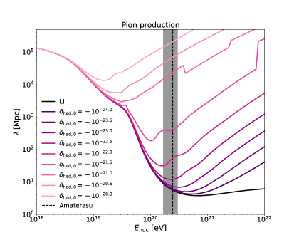
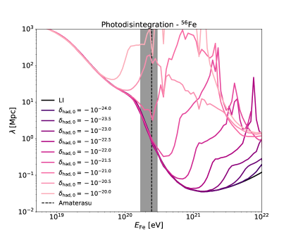
Figure 1: Mean free path as a function of the energy for different LIV scenarios. The different colors represent scenarios with increasing LIV coefficients. The vertical dashed line and shaded area show the detected energy for Amaterasu and the range of systematic uncertainties. The top and bottom panels are for photopion production and photodisintegration for an iron nucleus, respectively. The calculations consider the Gilmore model for the EBL background [19].

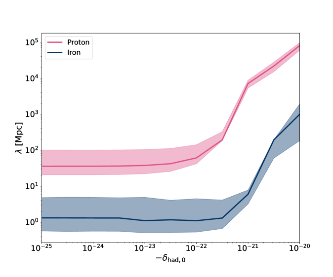
Figure 2: Mean free path as a function of the LIV coefficient for the detected energy of Amaterasu. The bracketing hypotheses of a primary proton and primary iron are considered. The shaded areas represent the results for different energies within the systematic uncertainties. The calculations consider the Gilmore model for the EBL background [19].

3 Combined fit under LIV assumptions

If LIV is present, it should not be a unique characteristic of a single event but an effect perceived by every particle. For that reason, an LIV scenario that softens the tension about the origin of Amaterasu should still be consistent with the remaining of experimental data, i.e., it still requires an astrophysical model that describes under the same LIV assumption the other events measured by the Telescope Array experiment. Hence, we present a combined fit of the spectrum and composition data measured by the Telescope Array under different LIV scenarios.

3.1 Dataset and fit method

Following [20], we use the 9-year Telescope Array energy spectrum [21] and depth of shower maximum, $X_{\rm{max}}$, distributions [22]. The spectral counts are divided into 10 bins per decade of energy, ranging from $10^{18.8}$ eV to $10^{20.4}$ eV. The $X_{\rm{max}}$ counts are divided into 4 main energy bins ($18.8<\log_{10}(E/\rm{eV})<19.0$, $19.0<\log_{10}(E/\rm{eV})<19.2$, $19.2<\log_{10}(E/\rm{eV})<19.6$ and $19.6<\log_{10}(E/\rm{eV})<20.0$) and then into 21 linear bins of $X_{\rm{max}}$, ranging from 590 to 1010 $\rm{g/cm^{2}}$. Amaterasu does not influence the $X_{\rm{max}}$ counts as it was only detected with the surface array (SD).

The combined fit was based on a widely used procedure [20, 23, 24, 15]. We simulate UHECR propagation using the state-of-the-art Monte Carlo package CRPropa3 [25]. The LIV effects were taken into account by implementing the modified mean free paths for each considered value of $\delta_{\rm{had},0}$ in the code. Sources were initially considered in a 3-D grid of energy, distance and particle primary. The energies were divided into 50 bins per decade, ranging from $10^{18}$ to $10^{22}$ eV. The distances were divided into 118 logarithmic bins, ranging from 3 to 3342 Mpc. Five representative primaries were considered: proton, helium, nitrogen, silicon, and iron. Since no arrival direction data is considered, a 1-D simulation in which no effect of magnetic fields is taken into account was performed. For each LIV coefficient value, $10^{4}$ events were simulated in each bin of the 3-D grid, resulting in a total of 118.59 million events for each LIV scenario. The information about the particle’s energy and species at the source, $E_{s}$, $I_{s}$, the source distance $D_{s}$ and energy and species at Earth, $E_{E}$, $I_{E}$ was recorded.

The fiducial astrophysical model considers every source accelerating particles as a standard candle with an injected spectrum given by

$$\left.\frac{dN}{dE_{s}}\right|_{i_{s}}=N_{0}f_{i_{s}}\left(\frac{E_{s}}{1\,\rm{EeV}}\right)^{-\Gamma}e^{-E_{s}/(Z_{i}R_{\rm{max}})},$$ (3.1)

where $i_{s}$ denotes the particle species at the source, and the spectral index, $\Gamma$, the maximum rigidity at the sources, $R_{\rm{max}}$ and the initial primary fractions, $f_{i_{s}}$, are free parameters to be fitted. The normalization, $N_{0}$, is taken such that the simulated flux matches the data for $E=10^{18.95}$ eV.

The $X_{\rm{max}}$ distributions are obtained by convoluting the Gumbel distributions [26] for each primary and energy arriving on Earth with the $X_{\rm{max}}$ acceptance given in [20]. The EPOS-LHC model [27] was considered for the hadronic interactions.

The combined fit was performed both by considering and not considering Amaterasu. For both the spectrum and $X_{\rm{max}}$ counts the likelihood for Poisson distributions was calculated and compared to the likelihood of a model that perfectly describes the data, resulting in the so-called deviance, which can be seen as a more generalized $\chi^{2}$ distribution. Seven free parameters and 16 (17) spectral and 55 $X_{\rm{max}}$ bins with non-zero counts considered for the case without (with) Amaterasu, leading to 64 (65) number of degrees of freedom (NDF).

The systematics in the energy scale and in the $X_{\rm{max}}$ were investigated by performing the fit again with the measured data scaled with $E\rightarrow E\pm 22\%$ and $X_{\rm{max}}\rightarrow X_{\rm{max}}\pm 15\,\rm{g/cm^{2}}$, resulting in 2x9 total fits for each LIV parameter.

3.2 Fit results

For all the fits, the best deviance was found with the systematic shift of $E\rightarrow E-22\%$ and $X_{\rm{max}}\rightarrow X_{\rm{max}}+15\,\rm{g/cm^{2}}$.

Figure 3 and figure 4 show the best-fit spectra and $X_{\rm{max}}$ distributions on Earth in an LI scenario and in a LIV scenario with $\delta_{\rm{had},0}=-10^{-22}$, respectively. The recovery at the high-energy end of the spectrum is significant and comes from the fact that, as previously discussed, protons undergo fewer interactions. The intermediate and low energy ranges of the proton spectrum are very similar for both cases. This creates a scenario that still describes well the low-energy end of the spectrum, which dominates the statistics while improving the description of the highest energy events. Even though the fit favors a proton-dominated scenario, the differences in the heavier components are noteworthy. Intermediate-mass nuclei such as helium and nitrogen have a larger contribution in the LIV case, since these particles experience less photodisintegration.

The differences for the $X_{\rm{max}}$ are smaller since the fluorescence detector (FD) measurements do not reach the highest energies, at which LIV effects are more significant. The difference seen in the first energy bin comes from the larger contribution of helium and nitrogen in the LIV case.

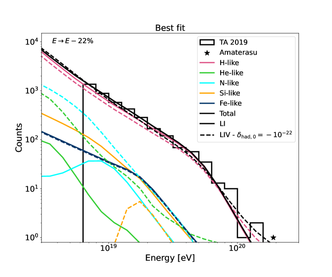
Figure 3: Spectra for the best fit. The different colors represent the contribution of different primaries at Earth and are divided into H-like ($A=1$), He-like ($2\leq A\leq 4$), N-like ($5\leq A\leq 22$), Si-like ($23\leq A\leq 38$), and Fe-like ($39\leq A\leq 56$). The dashed and full lines are for the LI case and the LIV case with $\delta_{\rm{had,0}}=-10^{-22}$ respectively. For both cases, the best fit was found with a systematic shift of $E\rightarrow E-22\%$ and $X_{\rm{max}}\rightarrow X_{\rm{max}}+15\,\rm{g/cm^{2}}$.

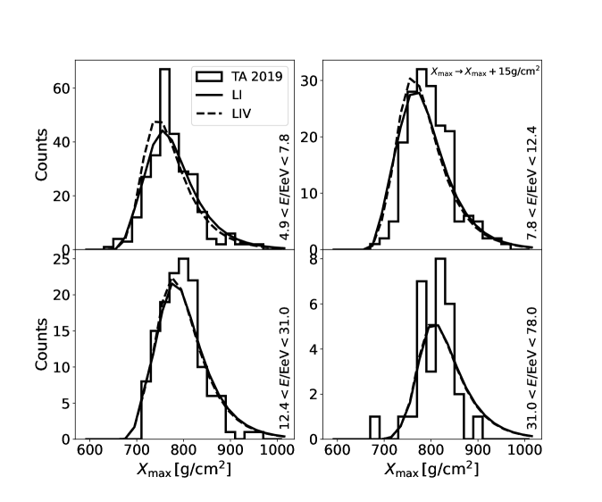
Figure 4: $X_{\rm{max}}$ distributions for the best fit. The dashed and full lines are for the LI case and the LIV case with $\delta_{\rm{had,0}}=-10^{-22}$ respectively. Each panel represents a different energy bin. For both cases, the best fit was found with a systematic shift of $E\rightarrow E-22\%$ and $X_{\rm{max}}\rightarrow X_{\rm{max}}+15\,\rm{g/cm^{2}}$.

Figure 5 shows the likelihood contour for the fit of these two cases. The presence of LIV shifts the region of the phase space that best fits the data. This is best quantified in figure 6, in which the evolution of the fit parameters with the LIV coefficients is shown. In stronger LIV scenarios, the cutoff cannot be well described by the energy-dependent propagation horizon and, thus, a model with a lower maximum power of acceleration at the sources is favored. As already shown in previous combined fit works [23, 15], the best spectral index is strongly correlated to the best rigidity cutoff. This behavior is also seen here, with the best-fit spectral index getting smaller for larger LIV coefficients. The primary fractions do not strongly vary, with a proton-dominated scenario being favored in all the considered scenarios. It is, though, noteworthy that the primary fraction as defined in this work refers to the fraction at the sources from energies below the rigidity cutoff. As the cutoff is rigidity (and not energy) dependent, for energies above $R_{\rm{max}}$, the injected composition becomes less proton-dominated and, thus, heavier.

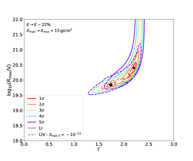
Figure 5: Left: Likelihood contour for the fit. The different colors show the contours for 1, 2, 3, 4, and $5\sigma$. The full and dashed lines are for the cases with LI and $\delta_{\rm{had,0}}=-10^{-22}$, respectively. The star and plus markers show the minimum for these respective cases. Right: best-fit primary fractions, $f_{i_{s}}$ for each LIV coefficient. In every scenario, the best fit was found with a systematic shift of $E\rightarrow E-22\%$ and $X_{\rm{max}}\rightarrow X_{\rm{max}}+15\,\rm{g/cm^{2}}$.

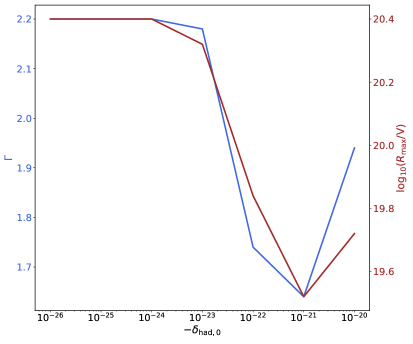
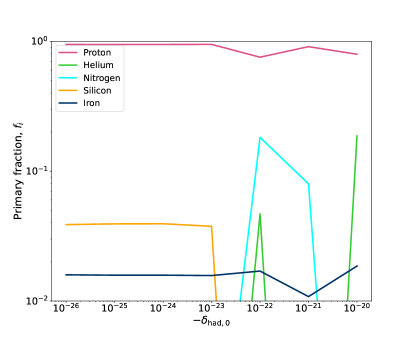
Figure 6: Left: Likelihood contour for the fit. The different colors show the contours for 1, 2, 3, 4, and $5\sigma$. The full and dashed lines are for the cases with LI and $\delta_{\rm{had,0}}=-10^{-22}$, respectively. The star and plus markers show the minimum for these respective cases. Right: best-fit primary fractions, $f_{i_{s}}$ for each LIV coefficient. In every scenario, the best fit was found with a systematic shift of $E\rightarrow E-22\%$ and $X_{\rm{max}}\rightarrow X_{\rm{max}}+15\,\rm{g/cm^{2}}$.

While figure 3 provides a visual indication of the improvement of the description of the data within LIV assumptions, a more quantitative measurement is needed. Figure 7 shows the evolution of the deviance with the LIV coefficient, both with and without considering Amaterasu. Even without Amaterasu, LIV scenarios are favored due to their better description of the high-energy end of the spectrum. With Amaterasu, the improvement of an LIV description becomes even more significant.

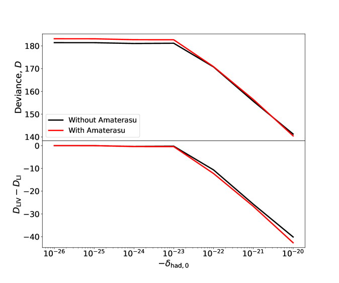
Figure 7: Deviance for the best fit found for each LIV coefficient. Black and red lines show the results not considering and considering the measurement of Amaterasu, respectively. The bottom panel shows the relative deviance to the LI case.

4 Conclusions

In this work, we explored the potential of describing the intriguing measurement of the Amaterasu particle under a LIV scenario.

At first, the kinematics of propagation interactions of UHECR under a phenomenological approach to LIV in the hadronic sector were calculated. The main effect for $\delta_{\rm{had},0}<0$ is a significant increase of the mean free path above an energy that is dictated by the LIV coefficient. The increase in the total mean free path for the energy of Amaterasu becomes significant for $-\delta_{\rm{had},0}>10^{-22}$. Even for the least conservative case, iron, the total mean free path can increase from a few Mpc to hundreds of Mpc. This would soften the tension with the origin of Amaterasu since no nearby (up to few tens of Mpc) strong source in the local void would be required to have accelerated it. This is robust within systematic uncertainties on the energy of Amaterasu.

Nevertheless, a LIV scenario that softens that tension still must be consistent with the rest of the data. For that reason, we performed a combined fit of the spectrum and composition data of Telescope Array for each LIV coefficient considered. The systematic uncertainties in the energy and $X_{\rm{max}}$ were taken into account by shifting the measured data by $E\rightarrow E\pm 22\%$ and $X_{\rm{max}}\rightarrow X_{\rm{max}}\pm 15\,\rm{g/cm^{2}}$. For every fit performed, the deviance was the lowest for $E\rightarrow E-22\%$ and $X_{\rm{max}}\rightarrow X_{\rm{max}}+15\,\rm{g/cm^{2}}$.

The best-fit spectra for $-\delta_{\rm{had,0}}>10^{-22}$ describe the low and intermediate energy range of the measured energy spectrum as well as the LI case while improving the description of the highest energy events. A lower rigidity cutoff is preferred by strong LIV scenarios, leading the spectrum cutoff that is dominated by the power of acceleration of the sources, since the propagation horizon is significantly increased.

Even without Amaterasu, the deviance of the best fit is improved under LIV assumptions. This result is consistent with the findings of the Pierre Auger Collaboration in their investigation of LIV effects in their data [15]. The simplistic astrophysical model considered in these works could be the reason behind that. Nevertheless, the need for a model in which less energy losses happen at the highest energies is once more raised with the results here presented. However, such a model can still be consistent with standard physics if, e.g., the relative predominance of the local sources is larger.

With Amaterasu, the improvement in the deviance is even larger, confirming that a LIV model in which the tension with the origin of Amaterasu is softened is still consistent and robust with the rest of the data from the Telescope Array.

With that, LIV is raised as a robust and plausible explanation for the unexpected Amaterasu particle. A better understanding of theoretical and phenomenological aspects such as astrophysical models for the UHECR sources and modeling of the galactic and extra-galactic magnetic fields, as well as further experimental developments and studies such as future analysis of the Telescope Array energy calibration and an improved understanding of its energy scale with relation to other experiments are needed to draw stronger conclusions.

References

- [1] Telescope Array collaboration, An extremely energetic cosmic ray observed by a surface detector array, Science 382 (2023) abo5095 [2311.14231].
- [2] HIRES collaboration, Detection of a cosmic ray with measured energy well beyond the expected spectral cutoff due to cosmic microwave radiation, Astrophys. J. 441 (1995) 144 [astro-ph/9410067].
- [3] R.G. Lang, A.M. Taylor, M. Ahlers and V. de Souza, Revisiting the distance to the nearest ultrahigh energy cosmic ray source: Effects of extragalactic magnetic fields, Phys. Rev. D 102 (2020) 063012 [2005.14275].
- [4] M. Unger and G.R. Farrar, Where Did the Amaterasu Particle Come From?, Astrophys. J. Lett. 962 (2024) L5 [2312.13273].
- [5] R.B. Tully, E.J. Shaya, I.D. Karachentsev, H.M. Courtois, D.D. Kocevski, L. Rizzi et al., Our Peculiar Motion Away from the Local Void, Astrophys. J. 676 (2008) 184 [0705.4139].
- [6] R. Jansson and G.R. Farrar, The Galactic Magnetic Field, Astrophys. J. Lett. 761 (2012) L11 [1210.7820].
- [7] R. Jansson and G.R. Farrar, A New Model of the Galactic Magnetic Field, Astrophys. J. 757 (2012) 14 [1204.3662].
- [8] Planck collaboration, Planck intermediate results.: XLII. Large-scale Galactic magnetic fields, Astron. Astrophys. 596 (2016) A103 [1601.00546].
- [9] D. Mattingly, Modern tests of Lorentz invariance, Living Rev. Rel. 8 (2005) 5 [gr-qc/0502097].
- [10] R.G. Lang, H. Martínez-Huerta and V. de Souza, Ultra-High-Energy Astroparticles as Probes for Lorentz Invariance Violation, Universe 8 (2022) 435.
- [11] S.T. Scully and F.W. Stecker, Lorentz Invariance Violation and the Observed Spectrum of Ultrahigh Energy Cosmic Rays, Astropart. Phys. 31 (2009) 220 [0811.2230].
- [12] X.-J. Bi, Z. Cao, Y. Li and Q. Yuan, Testing Lorentz Invariance with Ultra High Energy Cosmic Ray Spectrum, Phys. Rev. D 79 (2009) 083015 [0812.0121].
- [13] L. Maccione, A.M. Taylor, D.M. Mattingly and S. Liberati, Planck-scale Lorentz violation constrained by Ultra-High-Energy Cosmic Rays, JCAP 04 (2009) 022 [0902.1756].
- [14] R.G. Lang for the Pierre Auger Collaboration, Testing Lorentz Invariance Violation at the Pierre Auger Observatory, PoS ICRC2019 (2019) 450.
- [15] Pierre Auger collaboration, Testing effects of Lorentz invariance violation in the propagation of astroparticles with the Pierre Auger Observatory, JCAP 01 (2022) 023 [2112.06773].
- [16] S. Coleman and S.L. Glashow, High-energy tests of Lorentz invariance, Phys. Rev. D 59 (1999) 116008.
- [17] S. Coleman and S.L. Glashow, Cosmic ray and neutrino tests of special relativity, Physics Letters B 405 (1997) 249.
- [18] R.G. Lang, Effects of Lorentz invariance violation on the ultra-high energy cosmic rays spectrum, 2017. 10.11606/D.76.2017.tde-13042017-143220.
- [19] R. Gilmore, R. Somerville, J. Primack and A. Dominguez, Semi-analytic modeling of the EBL and consequences for extragalactic gamma-ray spectra, Mon. Not. Roy. Astron. Soc. 422 (2012) 3189 [1104.0671].
- [20] Telescope Array collaboration, Telescope Array Combined Fit to Cosmic Ray Spectrum and Composition, PoS ICRC2021 (2021) 338.
- [21] Y. Tsunesada, T. Abuzayyad, D. Ivanov, G. Thomson, T. Fujii and D. Ikeda, Energy Spectrum of Ultra-High-Energy Cosmic Rays Measured by The Telescope Array, PoS ICRC2017 (2018) 535.
- [22] D. Bergman and T. Stroman, Telescope Array measurement of UHECR composition from stereoscopic fluorescence detection, PoS ICRC2017 (2018) 538.
- [23] Pierre Auger collaboration, Combined fit of spectrum and composition data as measured by the Pierre Auger Observatory, JCAP 04 (2017) 038 [1612.07155].
- [24] Pierre Auger collaboration, Constraining models for the origin of ultra-high-energy cosmic rays with a novel combined analysis of arrival directions, spectrum, and composition data measured at the Pierre Auger Observatory, JCAP 01 (2024) 022 [2305.16693].
- [25] R. Batista, A. Dundovic, M. Erdmann, K.-H. Kampert, D. Kuempel, G. Müller et al., CRPropa 3 - a Public Astrophysical Simulation Framework for Propagating Extraterrestrial Ultra-High Energy Particles, JCAP 05 (2016) 038 [1603.07142].
- [26] M. De Domenico, M. Settimo, S. Riggi and E. Bertin, Reinterpreting the development of extensive air showers initiated by nuclei and photons, JCAP 07 (2013) 050 [1305.2331].
- [27] T. Pierog, I. Karpenko, J. Katzy, E. Yatsenko and K. Werner, EPOS LHC: Test of collective hadronization with data measured at the CERN Large Hadron Collider, Phys. Rev. C 92 (2015) 034906 [1306.0121].