On Isolated Hypersurface Singularities: Algebra-geometric and symplectic aspects.
Notes of the 2022–2023 Leiden seminar.

Introduction

Context and origin of the notes

These notes are based on a seminar which took place in the autumn of 2022 at the Mathematical Institute of the University of Leiden. Its goal was to understand the recent preprint [EL21] by J. Evans and Y. Lekili, a follow-up of the papers [LU21, FU11], in which the symplectic cohomology of the Milnor fiber for specific classes of isolated singularities has been calculated.

What attracted us to this paper is first of all the interplay between the algebra-geometric and symplectic techniques, a relatively new feature, perhaps going back to the article [McL16] by M. McLean. In [EL21] the algebraic geometry is related to threefold singularity theory as taken up in the 1980ies and 1990ies by M. Reid, J. Kollàr e.a., but which still is an active area of research. The symplectic techniques involve quite disparate inputs, about which more later on. The basic relation with singularities comes from the natural symplectic structure on the Milnor fiber of an isolated hypersurface singularity and the natural contact structure on its link.

The main motivating question is: ”what implications have symplectic and contact invariants for algebra-geometric phenomena of a singularity?” Note that symplectic and contact invariants are (much) finer than topological invariants, but much harder to calculate. Only recently this has been achieved for several classes of isolated hypersurfaces, in particular in the above mentioned papers.

One of the striking new results of [EL21] is the computation of contact invariants for the link of some of these singularities. As a result, contact structures for certain diffeomorphic links in dimension $5$ could be distinguished using these invariants.

On the algebra-geometric side there is a (largely conjectural) interplay between symplectic invariants and the existence of a so-called small resolution. For several threefold singularities a precise conjecture in this direction has been resolved, another striking result of [EL21].

Some historical background

Singularity theory in complex and differential geometry is a fairly old and well-established branch of mathematics. See e.g. [AVGL98, Mil63]. In differential geometry the object of study consists of the critical points of a function $f:M\to{\mathbb{R}}$, where $M$ is some differential manifold. A point $m\in M$ is critical if $df(m)=0$. Considering second order derivatives one introduces the Hessian at $m$, a certain real quadratic form. Then $m$ is said to be non-degenerate if the Hessian at $f$ is non-degenerate. If all critical points of $f$ are non-degenerate, then $f$ is called a Morse function. Choosing a metric on $M$, one associates to the Morse function $f$ its gradient vector field $\nabla(f)$. The Betti numbers of $M$ can now be estimated, and in some cases calculated, following the flow of $\nabla(f)$, using the indices of the Hessians at the various critical points of $f$. See for instance [Mil63].

Associating to an index $k$ critical point a $k$-cell, the free ${\mathbb{Z}}$-module on these cells can be made into a homological complex by defining the boundary operators using the flow of $\nabla(f)$. This idea is due to S. Smale [Sma60] and others as explained in R. Bott [Bot88]. See [Hut02] for an introduction to these ideas. In section 5.3.A, the reader finds a summary of it as a warm-up for a variant called symplectic cohomology. The essential ingredient here is Floer (co)homology named after A. Floer [Flo88]. Originally Floer’s approach played an important role for the understanding of the topology of $3$- and $4$-manifolds. A. Floer and H. Hofer in [FH94], and A. Floer, K. Cieliebak, H. Hofer in [CFH95] extended these ideas to the symplectic world. Taking limits in various ways the resulting symplectic (co)homology groups comes in different flavors depending on the precise context of the applications. Whatever version one chooses, these groups are notably hard to calculate.

Very recently it has been realized that for singularities defined by functions $w_{A}:{\mathbb{C}}^{n+1}\to{\mathbb{C}}$ with a critical point at ${\bf\it 0}$, coming from invertible matrices $A=(a_{ij})\in\operatorname{\mathsf{G}L}_{n+1}({{\mathbb{C}}})$ (see Eqn. (1.1)), one can define Hochschild cohomology of the associated category of matrix factorizations. On the other hand, these singularities give rise to certain Fukaya categories and their mirror-duals related to their symplectic geometry as sketched in Section 8.2 of these notes. Homological mirror symmetry in this case consists in replacing $A$ by its transpose and conjecturally the Hochschild cohomology of the category of matrix factorizations for $A$ is the same as the symplectic cohomology for the Milnor fiber of the singularity $\{w_{{A}^{{\mathsf{T}}}}=0\}$. This prediction from homological mirror symmetry has been proven for several kinds of these singularities, cf. Proposition 8.8. Since Hochschild cohomology is amenable to explicit calculation, in these cases symplectic cohomology for the Milnor fiber of the corresponding IHS can be calculated as well. Moreover, there is an extra algebraic structure present on Hochschild cohomology, that of a Gerstenhaber algebra. One of the main results of [EL21] states that this leads to a contact invariant for the link of large classes of such singularities.

About the seminar

Special attention was given to so called small resolutions of special singularities. See Section 3.3 for the algebra-geometric background and and 3.5 for the above mentioned (conjectural) relation with symplectic geometry. It turns out that this area presents a fascinating source of examples for the interplay of algebraic geometry and symplectic geometry.

Evans and Lekili use the above discussed recent techniques from homological mirror-symmetry in their paper. The participants in the seminar have various backgrounds and specializations in algebraic geometry and/or symplectic geometry but were not familiar with all of these techniques. In the seminar the required results from these fields were then treated as a black box, with the exception of the elaborate input from matrix factorizations.

Such an ambitious program with inputs from rather disparate field makes access difficult. So the idea arose to work out the talks to make the results from [EL21] more accessible to both algebraic and symplectic geometers. This unavoidably implies that some chapters might be well known to either one of these groups, but the participants of the lectures all felt that such a text would serve the greater goal of introducing the mathematical community to this exiting and challenging intersection of two fields dealing with singularities from totally different angles.

The resulting notes presented here entirely reflect my view as an algebraic geometer well versed in the older differential geometric literature, but a dilettant in matters of symplectic geometry and the finer points of matrix factorizations, especially their categorical aspects.

The writing up of these notes proceeded in parallel with a project on cDV-type singularities related to small resolutions by three of the speakers of the seminar, and whose outcome is the recent preprint [APZ24]. I could not resist explaining (at the end of Section 3.5) some of the enticing new results they obtained.

Acknowledgement

In writing this extended version I have had several long explanatory discussions with the participants of the seminar, N. Adaglou, F. Pasquotto, A. Sauvaget and A. Zanardini for which I want to thank them. I also want to thank Thomas Dyckerhoff for explaining some points of [Dyc11] and M. Hablicsek for help with Hochschild cohomology of dg-categories.

List of Notation

Symbol	meaning	page
IHS	isolated hypersurface singularity	1.1
$w_{A}=0$	invertible polynomial IHS	1.1
$\mathsf{L}_{X,x}$	link of the singularity germ $(X,x)$	1.2
$\mathsf{F}_{f}=\mathsf{F}_{X,x}$	Milnor fiber of
	the singularity germ $(X,x)$, $X=\{f=0\}$	1.2
$\mu(w)=\mu(X,x)$	Milnor number of
	the singularity germ $(X,x)$, $X=\{f=0\}$	1.3
$\mathsf{Jac}_{w}$	Jacobian ring of $w\in{\mathbb{C}}[x_{1},\dots,x_{m+1}]$	1.3
$T^{*}U$	total space of
	the cotangent bundle of the manifold $U$	1
$\lambda_{\rm can},\omega_{\rm can}$	canonical $1$ and $2$ form on $T^{*}U$	1
$\omega_{C^{n}}$	canonical symplectic form on ${\mathbb{C}}^{n}$	1.4
$\mathsf{SH}^{*}(\mathsf{F}_{X,x})$	symplectic cohomology of the germ $(X,x)$	1.13
$\mathsf{HH}^{*}(A,\Gamma_{A})$	Hochschild cohomology associated to
	the matrix $A$ and group $\Gamma_{A}$	1.5.A
$A_{1,2k}$, $\alpha_{1,k}$	cDV-singularity $A_{1}(2k)$ and its link	1.16
$\operatorname{\mathsf{B}l}_{V}({W})$	blow up of smooth variety $W$ in subvariety $V$	2.2
$T_{U},T^{*}_{U}$	tangent, resp. cotangent bundle of $U$	3.1
$\omega_{Z}$, $K_{X}$	canonical sheaf, canonical divisor of $X$	3.1
$\mathsf{Cl}_{x}(X)$, $\rho(x)$	local class group of $(X,x)$ and its rank	1
$\iota_{Y}$	contraction against vector field $Y$	1
${\mathcal{L}}_{Y}$	Lie derivative in direction of vector field $Y$	4.1.B
$R_{\alpha}$	Reeb vector field for contact form $\alpha$	4.2.B
$\mathsf{Cyl}{(M_{\alpha})}$	symplectization of contact manifold $(M,\alpha)$	4.2.C
$\widehat{W}$	symplectic completion of Liouville domain $W$	4.2.D
$\operatorname{\mathsf{S}p}({V}),\,\operatorname{\mathsf{S}p}({2n})$	symplectic group of $V\simeq{\mathbb{R}}^{2n}$	5.1
$\mu(\psi)$	Maslov index of path $\psi$ in $\operatorname{\mathsf{S}p}({2n})$	5.1
$\operatorname{\mu_{\mathsf{C}Z}}({H,{{\bf\it x}}})$	Conley–Zehnder index
	of smooth curve ${{\bf\it x}}$ of Hamiltonian flow of $H$	5.3
$C_{*}^{\rm Morse}M$	Morse chain groups of manifold $M$	5.3.A
$H_{*}^{\rm Morse}(M),H^{*}_{\rm Morse(M)}$	Morse (co)homology of manifold $M$	5.3.A
$\mathsf{CF}^{*}(H)$	Floer chain groups of Hamiltonian $H$	5.6
$\mathsf{HF}^{*}(\widehat{W},H)$	Floer cohomology of Hamiltonian $H$
	on completion of Liouville domain $W$	5.3.B
$\mathsf{SH}^{*}(\widehat{W})^{<a}$	symplectic cohomology of $\widehat{W}$
	w.r. periodic orbits of periods $<a$	5.3.B
$\mathsf{SH}^{*}(W)$	symplectic cohomology of $W$	5.3.B
$\mathsf{CF}^{\pm}_{*}(H)$	positive/negative Floer
	chain groups of Hamiltonian $H$	5.3.C
$\mathsf{SH}^{k}_{\pm}(W)$	positive/negative Floer
	cohomology of $W$	5.3.C
$md(X,x)$	minimal discrepancy
	the singularity germ $(X,x)$	5.14
$\text{hmi}(\mathsf{L}_{X,x},\xi),\text{hmi}(\mathsf{L}_{X,x},\xi)$	(highest) minimal index of the link
	of the singularity germ $(X,x)$	5.17
$N^{\bullet}({{\bf\it f}})$	Koszul sequence for $R$-regular sequence	6.2
$\{{{\bf\it f}},{{\bf\it g}}\}$	Koszul matrix factorization w.r. to ${{\bf\it f}}$, ${{\bf\it g}}$	2
$\underline{C}(R)$	category of complexes over $R$	6.7
$\underline{C}_{dg}(R)$	dg-category of complexes over $R$	6.3.B
$[\underline{A}]$	homotopy category of $\underline{A}$	6.3.B
$\underline{Mat\!f}_{R,w},\underline{Mat\!f}_{R,w}^{\infty}$	category of matrix factorisations of $w\in R$	6.3.C
$M^{\rm stab}$	stabilization of $M$	6.4.A
$X^{o}$-module $M$	$M$ with action of $X$ from the right	6.16
$\widehat{\underline{C}}$	”completion” of category $\underline{C}$	6.16
$\Delta$	diagonal of $R$ in $R\otimes_{k}R$, $R=k[\![x_{1},\dots,x_{m}]\!]$	6.4.D
$\mathsf{HH}^{*}(A)$	Hochschild cohomology of algebra $A$	6.5.A
$A^{o}$, $A^{e}$	opposite and enveloping algebra of $A$	6.5.A
$C^{\rm bar}_{*}(A)$	bar-complex of algebra $A$	6.5.A
$\underline{A}^{o}$, $\underline{A}^{e}$	opposite and enveloping dg-category of $\underline{A}$	• ‣ 6.5.B
$\Delta_{\underline{A}}$	diagonal/identity functor of dg-category $\underline{A}$	6.24
$\underline{Mat\!f}_{w,\Gamma,\chi}$	category of equivariant matrix
	factorizations of $w$ w.r. to $(\Gamma,\chi)$	6.27
$G_{A}$	kernel of character $\chi_{A}:\Gamma_{A}\to{\mathbb{C}}^{*}$	8.1
$\chi_{j}$	character of $\Gamma_{A}$	8.1
$\chi_{{\bf\it m}}$	character of $({\mathbb{C}}^{*})^{n+2}$	8.1
$A_{\gamma}$, $B_{\gamma}$, $C_{\gamma}$	sets of $\gamma$-monomials	(=case 1(b) of Prop. 6.29)): , (=case 1a of Prop. 6.29):
$\widetilde{G_{A}}$	auxiliary group	8.3

Chapter 1 Overall view

I shall work over the complex numbers and use the analytic topology unless mentioned otherwise.

1.1. The protagonists

A complex variety $V$ is a subset of ${\mathbb{C}}^{N}$ given by the vanishing of a finite number of holomorphic functions. One assumes throughout that $V$ has just one singularity at the origin ${\bf\it 0}\in{\mathbb{C}}^{N}$. Such isolated singularities are investigated in appropriately small balls centered at ${\bf\it 0}$. Special attention is given to isolated hypersurface singularities, abbreviated IHS in what follows. Explicitly,

Definition 1.1.

An $m$-dimensional analytic hypersurface

$$V(f):=\{{{\bf\it x}}=(x_{1},\dots,x_{n+1})\subset{\mathbb{C}}^{m+1}\mid f(x_{1},\dots,x_{m+1})=0\},\quad f({\bf\it 0})=0$$

has an isolated singularity at ${\bf\it 0}$ if there is an open neighborhood $U\subset{\mathbb{C}}^{m+1}$ of ${\bf\it 0}$ such that ${\bf\it 0}$ is the only zero of $\nabla f$ in $U$ along $V(f)$.

Examples 1.2.

1. The type $A_{n}$ singularities or double point singularities on curves: $x^{2}-y^{n+1}=0$, $n\geq 1$. For odd $n$ these have two branches $x=\pm y^{\frac{1}{2}(n+1)}$ (the red curve) and for $n$ odd only one (the black curve). The latter are the so-called cusps.

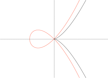
Figure 1.1. Double points.

2. The triple point curve singularities $D_{n}$ (given by $y(x^{2}-y^{n-2})=0$, $n\geq 4$), and the three $E$-types $x^{3}+y^{4}=0$, $x(x^{2}+y^{3})=0$ and $x^{3}+y^{5}=0$, respectively $E_{6},E_{7}$ and $E_{8}$.
3. The du Val surface singularities are obtained from the $A$-$D$-$E$-types by adding the square of a new variable. Adding more squares of new variables, then gives IHS of higher dimension, likewise called ”of $A$-$D$-$E$-type”.
4. The compound du Val threefold singularities, abbreviated cDV-singularities: $g(x,y,z)+th(x,y,z,t)$ by definition are such that the hyperplane $t=0$ gives a du Val surface singularity.
5. Singularities associated to invertible matrices. Consider the polynomial in ${\mathbb{C}}[x_{1},\dots,x_{m+1}]$ given by

(1.1) $$w_{A}({\bf\it x}):=\sum_{k}x_{1}^{a_{k,1}}x_{2}^{a_{k,2}}\cdots x_{m+1}^{a_{k,m+1}},\quad A=(a_{ij})\in\operatorname{\mathsf{G}L}_{m+1}({{\mathbb{C}}}).$$

If $w_{A}=0$ has an IHS at ${\bf\it 0}$, one speaks of an invertible polynomial IHS. This is the case for instance if $A$ is diagonal with exponents $\geq 2$. Note that the equations $\sum_{j}a_{ij}d_{i}=d$, $d\in{\mathbb{Q}}$, $i=1,\dots,m+1$, have a unique solution over the rationals. Clearing denominators, there is a unique solution $(d_{1},\dots,d_{m+1},d)$ with $d$ a positive integer and with $\gcd(d_{1},\dots,d_{m+1},d)=1$. If $A$ is diagonal, the IHS is called a Brieskorn–Pham singularity.

The polynomial $w_{A}$ is a so-called weighted homogeneous polynomial of type $(d,[d_{1},\dots,d_{m+1}])$, which means that if $t\in{\mathbb{C}}^{*}$ acts on ${\mathbb{C}}^{m+1}$ by multiplying $x_{j}$ by $t^{d_{j}}$, the induced action on polynomials sends $w_{A}$ to $t^{d}w_{A}$. The associated integer $\alpha(w_{A})=d-\sum d_{j}$ is called the amplitude of $w_{A}$. Its sign plays an important role in the theory: If $\alpha(w_{A})<0$ one calls $w_{A}$ a log-Fano type polynomial, if $\alpha(w_{A})=0$, it is of log-Calabi–Yau type, while a log-general type polynomial has $\alpha(w_{A})>0$.

1.2. Links and Milnor fibrations

For an $m$-dimensional isolated singularity $(X,x)\subset({\mathbb{C}}^{m+1},{{\bf\it 0}})$, not necessarily a hypersurface singularity, the link is defined as the $(2m-1)$-dimensional manifold which is obtained by intersecting $X$ with a small enough sphere centered at ${{\bf\it 0}}$:

$$\mathsf{L}_{X,x}:=X\cap S^{2m+1}({{\bf\it 0}},\epsilon),\quad 0<\epsilon\ll 1.$$

For all small enough $\epsilon$ the oriented diffeomorphism type of this manifold does not change.

In the hypersurface case $X=\{f=0\}\subset{\mathbb{C}}^{m+1}$ the map

$$S^{2m+1}({\bf\it 0},\epsilon)-\mathsf{L}_{X,x}\mathop{\vbox{\halign{ #\cr${\scriptstyle\hfil\;\;\phi_{f}\;\;\hfil}$\crcr\kern 2.0pt\nointerlineskip\cr\rightarrowfill\crcr}}\;}S^{1},\quad\phi_{f}({\bf\it x})=f({{\bf\it x}})/|f({{\bf\it x}})|$$

is well defined. J. Milnor shows [Mil68, Thm. 4.8] that $\phi_{f}$ is a differentiable locally trivial fiber bundle with smooth $2m$-dimensional fibers. The general fiber is called the Milnor fiber $\mathsf{F}_{f}=\mathsf{F}_{X,x}$ of the germ $(X,x)$ given by $f=0$. The topology of this fibration is well-understood especially if $f$ is a polynomial.

In these notes, I shall mostly use the letter $w$ for polynomial singularities.

Theorem 1.3 ([Mil68, §5]).

The Milnor fiber $\mathsf{F}_{w}$ and the link $\mathsf{L}_{w}$ of an isolated $m$-dimensional singularity of a polynomial singularity $w=0$ have the following properties:

1. $\mathsf{F}_{w}$ is (orientably) parallelizable, i.e its tangent bundle admits an orientation preserving trivialization;

2. $\mathsf{F}_{w}$ has the homotopy type of a wedge of $m$-spheres; in particular, its middle homology $H_{m}(\mathsf{F}_{w})$, $2m=\dim\mathsf{F}_{w}$, is free of rank $\mu(w)$;

3. Each fiber of the Milnor fibration $\phi_{w}$ has the link $\mathsf{L}_{w}$ as its boundary;

4. If $m\geq 2$, then $\mathsf{L}_{w}$ is $(m-2)$-connected, that is, it is connected and its homotopy groups $\pi_{k}(\mathsf{L}_{w})$ vanish for $k=1,\dots,m-2$;

5. $\mathsf{F}_{w}$ is $(m-1)$-connected.

The number $\mu(w)=\mu(X,x)$ of $m$-spheres in this theorem is called the Milnor number of the singularity germ $(X,x)$ given by $w=0$. It can also be calculated algebraically as the dimension of the Jacobian ring $\mathsf{Jac}_{w}$ of $w\in{\mathbb{C}}[x_{1},\dots,x_{m+1}]$:

(1.2) $$\mu(w)=\dim\mathsf{Jac}_{w},\,\mathsf{Jac}_{w}={\mathbb{C}}[x_{1},\dots,x_{m+1}]/J(w),\quad J(w)=\left(\frac{\partial w}{\partial x_{1}},\dots,\frac{\partial w}{\partial x_{m+1}}\right).$$

Using S. Smale’s technique of surgery there is a sharper statement in the case $m\not=2$. This sharper statement implies the existence of certain types of Morse functions on the Milnor fiber which play a crucial role later (cf. the statement of Corollary 7.7).

Let me first give a short explanation of this technique. One starts with an $m$-dimensional manifold with boundary $(W,\partial W)$ and such that $\partial W$ contains $S^{k-1}\times B^{m-k}$. More precisely, one assumes that there exists a smooth map

$$S^{k-1}\times B^{m-k}\mathop{\vbox{\halign{ #\cr${\scriptstyle\hfil\;\;\phi\;\;\hfil}$\crcr\kern 2.0pt\nointerlineskip\cr\rightarrowfill\crcr}}\;}\partial W.$$

Here $B^{s}\subset{\mathbb{R}}^{s}$ denotes the unit ball in ${\mathbb{R}}^{s}$. One attaches a $k$-handle $H^{k}=B^{k}\times B^{m-k}$ to $W$ by taking first the disjoint union of $W$ and $H^{k}$ and then glues $S^{k-1}\times B^{m-k}\subset\partial H^{k}$ to $\partial W$ using $\phi$. At the same time $B^{k}\times S^{m-k-1}$, the other part of the boundary of $H^{k}$, replaces the image of $\phi$ in $\partial W$:

$$(W^{\prime},\partial W^{\prime})=\left(W\cup_{\phi}H^{k},(\partial W-\text{Im}(\phi))\cup B^{k}\times S^{m-k-1}\right).$$

Then $W^{\prime}$ said to be obtained from $W$ by attaching the $k$-handle $H^{k}$ and $\partial W^{\prime}$ is obtained from $\partial W$ by an elementary surgery of type $(k,m-k)$. An $m$-manifold with boundary obtained by successively attaching handles (possibly of varying types) is called a handlebody.

Figure 1.2. Elementary surgery on $S^{1}$ of type $(1,1)$ and a typical Milnor fiber in (complex) dimension $1$ viewed as a handlebody.

In the present setting the Milnor fiber is $(m-1)$-connected and the link $(m-2)$-connected and in this situation Smale’s result [Sma62, Theorem 1.2] applies, yielding:

Theorem 1.4 ([Mil68, Thm. 6.6]).

If $m\not=2$ the Milnor fiber of an isolated $m$-dimensional singularity having Milnor number $\mu$ is obtained from the $m$-ball by attaching $\mu$ disjoint $m$-handles.

This indeed refines Milnor’s result: Attaching an $m$-handle to the $2m$-ball gives a manifold which is homeomorphic to the product $S^{m}\times D^{m}$ which has the $m$-sphere as a deformation retract and attaching $\mu$ disjoint $m$-handles has a wedge of $\mu$ such $m$-spheres as deformation retract. In Figure 1.2 the right hand picture is supposed to have connected boundary (the handles are all open at the back, making a large knot-like boundary). It represents the Milnor fiber of an irreducible $1$-dimensional singularity (see Section 2.3 for some background). However, in case the singularity has $k$ branches the boundary has $k$ connected components.

Before explaining the consequence for Morse functions, let me first recall the definition:

Definition 1.5.

Let $M$ be a smooth $n$-dimensional manifold, and $f:M\to{\mathbb{R}}$ a smooth function. A point $p\in M$ is a critical point if $df(p)=0$ and it is a non-degenerate critical point (of index $r$) if locally in a neighbourhood $U$ of $p$ coordinates $x_{1},\dots,x_{n}$ can be found centered at $p$ so that $f(x)=-\sum_{j=1}^{r}x_{j}^{2}+\sum_{j=r+1}^{n}x_{j}^{2}$ in $U$. The function $f$ is a Morse function if all critical points of $f$ are non-degenerate. The flow lines of the gradient vector field of $f$ is called the flow associated to the Morse function $f$.

In a precise sense ”most” smooth functions are More functions so that small perturbations of any smooth function gives a Morse function. The critical points of Morse functions and their indices can be used to describe a manifold by means of attaching handles which gives some information about the topology of the manifold. See [Mil63] for more information and many examples. Sometimes the information is ideal: there exists a so-called perfect Morse function with precisely $b_{r}(M)$ critical points of index $r$ for all $r$. This is the case for Milnor fibers of isolated hypersurface singularities:

Corollary 1.6.

In case the complex dimension $m$ is different from $2$, there exists a Morse function on the Milnor fiber with a minimum (index $0$) and $\mu$ non-degenerate critical points of index $m$.

Proof.

One starts off with the $2m$ ball $W_{0}$ with Morse-function $f_{0}:W_{0}\to[-3,-1]$ given by $f_{0}=-1-2\sum_{j=1}^{2m}x_{j}^{2}$ and then one consecutively attaches $m$-handles as follows.

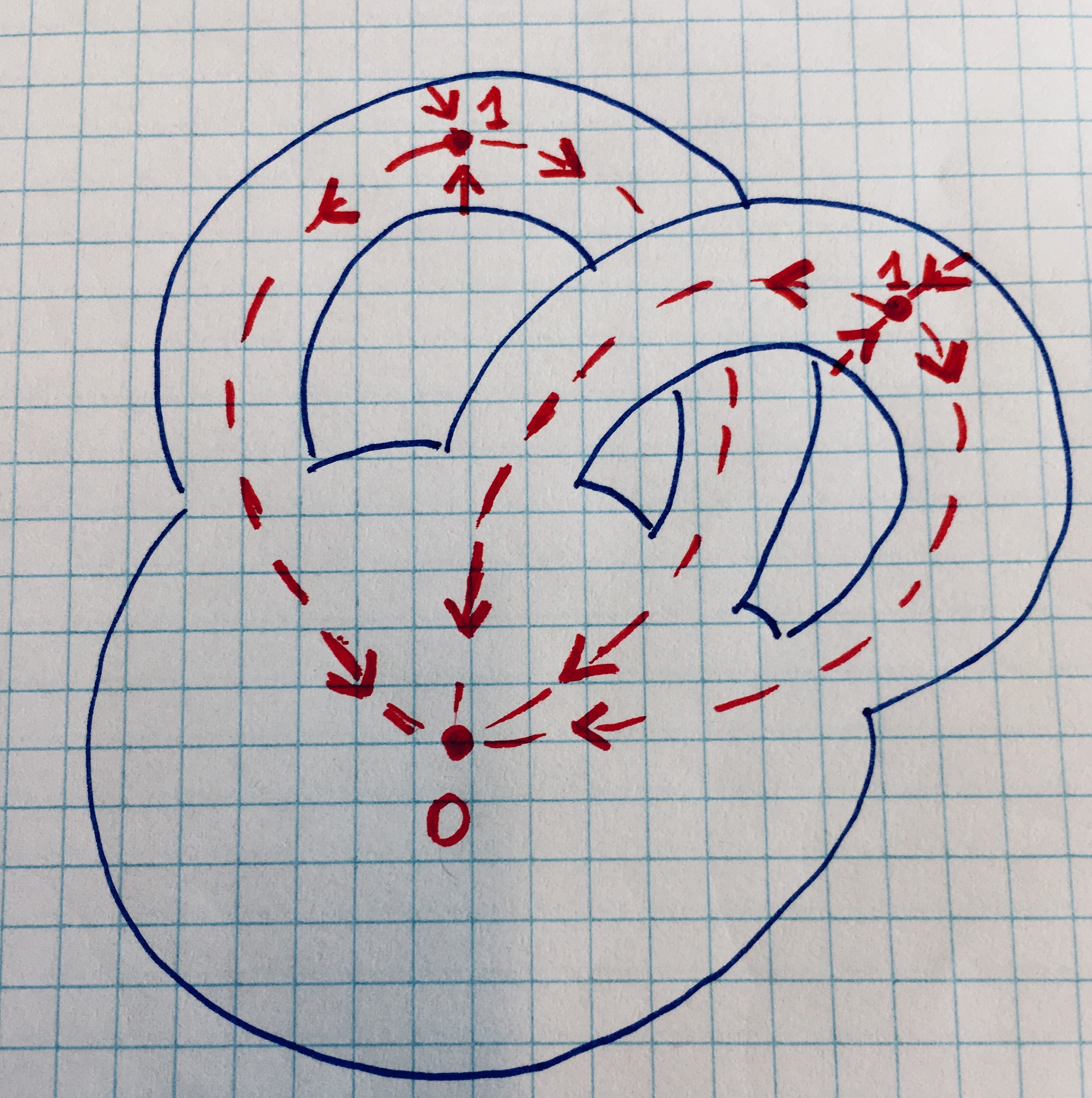
Figure 1.3. Handlebody with flow associated to the Morse function.

By [Mil65, Thm. 3.12] an elementary surgery of type $(m,m)$ applied to $\partial W_{0}$ is given by a manifold $W_{0\to 1}$ with ”lower” boundary $\partial W_{0}$ and Morse function $f_{01}:W_{0\to 1}\to[-1,1]$ having one non-degenerate critical point of index $m$ and being $-1$ on $\partial W_{0}$ and $1$ on the ”upper” boundary of $W_{0\to 1}$. Let $W_{1}=W_{0}\cup W_{0\to 1}$ be the $(2m)$-fold obtained from $W_{0}$ by attaching the $m$-handle produced by the elementary surgery. The functions $f_{0}$ and $f_{1}$ are both $0$ on $\partial W_{0}$ and by construction (see the proof of [Mil65, Thm. 3.12]) $f_{1}$ glues differentiably to $f_{0}$ without critical points near this boundary and so gives a Morse function $f_{1}:W_{1}\to[-1,1]$. A further elementary surgery of type $(m,m)$ applied to the upper boundary of $W_{0\to 1}$ gives the manifold $W_{2}$ which is obtained from $W_{1}$ by attaching an $m$-handle and which has a Morse function with one more critical point of index $m$ on the attached $m$-handle. Continuing in this manner one obtains a Morse function $f_{\mu}$ on the Milnor fiber with one critical point of index $0$ and $\mu$ critical points of index $m$, one for each attached handle. ∎

Example 1.7.

1. One can show that the link of the cusp $x^{2}-y^{3}=0$ is homeomorphic to a trefoil-knot given parametrically by $x=(2+\cos 3t)\cos 2t$, $y=(2+\cos 3t)\sin 2t$, $z=\sin 3t$.

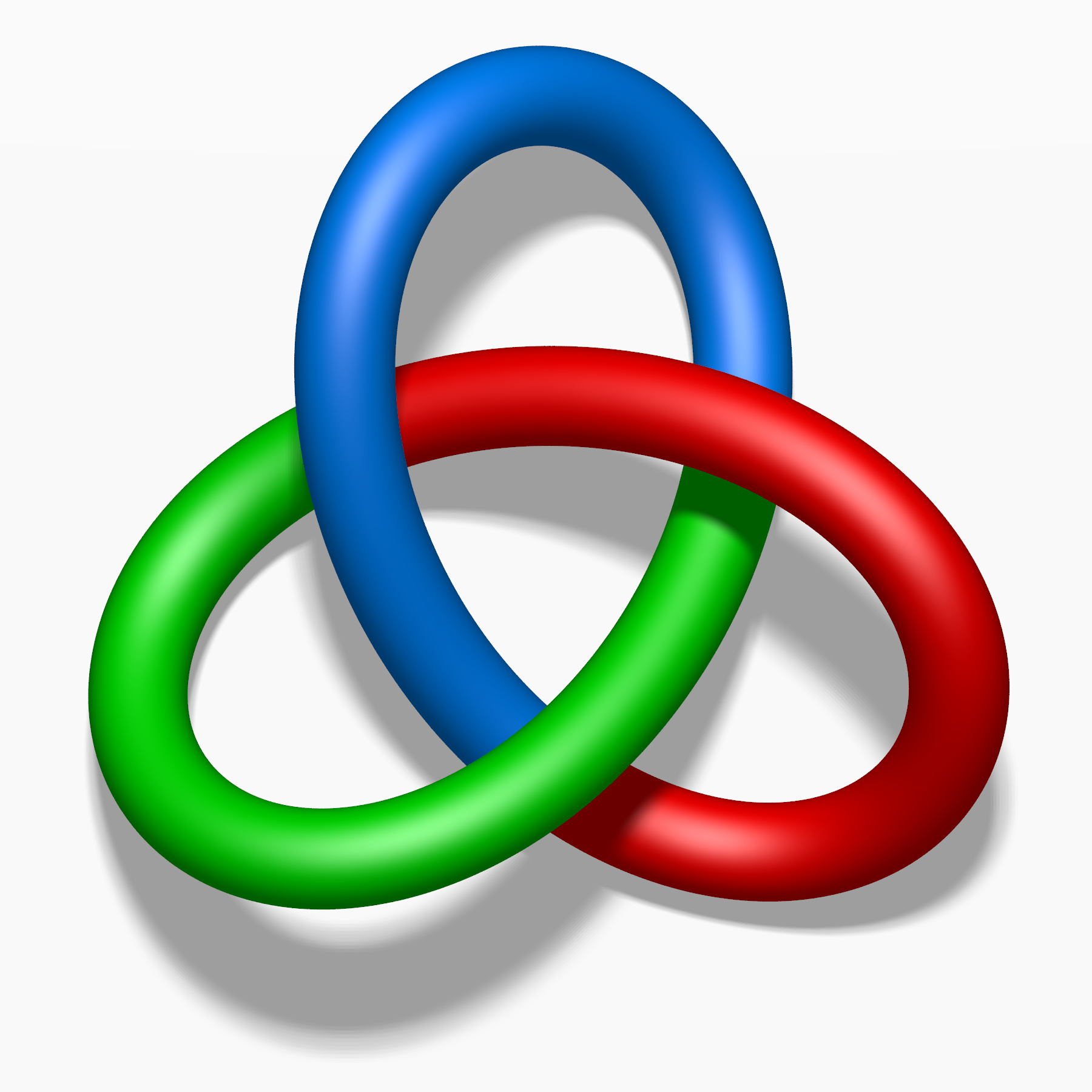
Figure 1.4. Disc bundle on trefoil knot (By Jim Belk - Own work, Public Domain,
https://commons.wikimedia.org/w/index.php?curid=7903214)

The Jacobian ring is spanned by $1$ and $y$ and so the Milnor number equals $2$. The Milnor fiber is diffeomorphic to a torus minus a disc spanning the trefoil knot. Hence the Milnor fiber contracts to the union of a latitudinal and longitudinal circle, i.e. a wedge of two circles.
2. Consider the singularity $z_{1}^{2}+z_{2}^{2}+z_{3}^{2}=0$. Its link can be calculated in real coordinates $x_{1},y_{1},x_{2},y_{2},x_{3},y_{3}$ given by $z_{j}=x_{j}+{{\bf\it i}}y_{j}$. Indeed the equation gives $\sum_{j}x_{j}^{2}-y_{j}^{2}=0$, $\sum_{j}x_{j}y_{j}=0$ and the sphere condition gives $\sum x^{2}_{j}+y^{2}_{j}=\epsilon^{2}$. Hence the link is given in ${\mathbb{R}}^{3}\times{\mathbb{R}}^{3}$ by the equations $\sum x_{j}^{2}=\sum y_{j}^{2}=\frac{1}{2}\epsilon^{2}$, ${{\bf\it x}}\cdot{{\bf\it y}}=0$ which gives the subset of the tangent bundle to $S^{2}$ consisting of tangent vectors of fixed length $\frac{1}{2}\sqrt{2}\epsilon$. This is also called the Stiefel manifold $\mathsf{St}(3,2)$. Similarly, for $\sum_{j=1}^{n+1}{{\bf\it z}}_{j}^{2}=0$ one obtains the bundle of tangent vectors to $S^{n}$ of fixed length, the Stiefel manifold $\mathsf{St}(n+1,2)$, an $S^{n-1}$-bundle over $S^{n}$. This is not always a product, but for $n=1,3,7$ it is (see [Ste51, §8.5 and §27], see also [Ada62]).

There is another way to view the Milnor fibration by considering a complex valued function $f$ defining an IHS at ${{\bf\it 0}}$ on a small enough ball $B=B({\bf\it 0},\epsilon)$. In a small enough disc $\Delta(0,r)$ the sets $F({{\bf\it x}},t):=\{f({{\bf\it x}})=t\}\cap B$ for $t\not=0$ are open subsets of $n$-dimensional algebraic varieties without singularities while $F({{\bf\it x}},0)$ is of course the defining IHS. Milnor shows in [Mil68, §5] that this yields an alternative incarnation of the Milnor fibration over the punctured disc. A more precise result of Lê states:

Theorem 1.8 ([Lê77]).

For $0<r\ll\epsilon\ll 1$, the family of (open) complex manifolds $\{f({{\bf\it x}})=t\}\cap\bar{B}({\bf\it 0},\epsilon)$ over the punctured disc $\Delta(0,r)-\{0\}$ is a locally trivial fiber bundle with fibers diffeomorphic to the Milnor fiber. Their boundaries are all diffeomorphic to the link $\mathsf{L}_{f}$.

1.3. Enter: the associated symplectic and contact structure

The Milnor fiber of an IHS has a canonical symplectic structure and its boundary, the link, inherits a canonical contact structure. This is briefly explained in this section. For more on these notions I refer to Chapter 4 and to the book [MS17] by D. McDuff and D. Salamon.

Definition 1.9.

1. A real $2$-form $\omega$ on a smooth manifold is non-degenerate if the skew form it defines on every tangent space is non-degenerate.
2. A symplectic structure on a smooth manifold $N$ is given by a closed non-degenerate real $2$-form $\omega$. A symplectic manifold is a smooth manifold equipped with a symplectic structure. A symplectomorphism $f:(N_{1},\omega_{1})\to(N_{2},\omega_{2})$ between symplectic manifolds $N_{1},N_{2}$, is a diffeomorphism such that $f^{*}\omega_{2}=\omega_{1}$. Two manifolds are called symplectomorphic if there is a symplectomorphism between them.
3. A contact structure on a smooth manifold $M$ of odd dimension $2n-1$ is a field $\xi$ of codimension $1$ hyperplanes in the tangent bundle of $M$ which defines a maximally non-integrable distribution. This means that at every point $m\in M$ two vector fields tangent to $\xi$ can be found whose Lie bracket is non-zero. A contact manifold is an odd-dimensional manifold admitting a contact structure. A contactomorphism is a diffeomorphism between contact manifolds preserving the contact structures. Two manifolds are called contactomorphic if there is a contactomorphism between them.

A one-form $\alpha$ such that $\mathop{\rm Ker}\nolimits(\alpha)=\xi$ is called a contact form. Locally in a chart with coordinates $x_{1},\dots,x_{2n-1}$ such a form exists: if $\displaystyle\sum a_{j}(x_{1},\dots,x_{2n-1})\frac{d}{dx_{j}}=0$ is a field of tangent hyperplanes, $\alpha=\sum_{j}a_{j}dx_{j}$ is a corresponding contact form. It is clearly unique up to multiplying with a function. This can be done globally, if $\xi^{\perp}$ can be oriented, i.e., if the normal vector field $\displaystyle\sum a_{j}\frac{d}{dx_{j}}$ can be scaled locally so that it glues to give a global normal vector to the field $\xi$ of hyperplanes. This is called a co-orientation. The corresponding form $\alpha$ is said to be induced by the chosen co-orientation. Note that if $\alpha$ is induced from a co-orientation, then $-\alpha$ is induced from the opposite co-orientation.

The contact structure being maximally non-integrable is equivalent to $\alpha\wedge(d\alpha)^{n}\not=0$. The non-uniqueness of the contact form of course holds globally: if two forms $\alpha,\alpha^{\prime}$ have $\xi$ as its kernel, $\alpha^{\prime}=f\cdot\alpha$ where $f$ is a nowhere zero function. Then $f>0$ precisely when both forms come from the same co-orientation.

Examples 1.10 (Symplectic manifolds).

1. The total space $T^{*}U$ of the cotangent bundle

   $$\pi:T^{*}U\to U,\quad U\text{ a smooth manifold}.$$

   Since the $1$-forms on $U$ are the sections of the cotangent bundle, there is a canonical $1$-form $\lambda_{\rm can}$ on $T^{*}U$ defined by

   (1.3) $$\lambda_{\rm can}(u,\alpha_{u})=\alpha_{u},\quad u\in U,\alpha_{u}\in T^{*}_{u}(U),$$

   and hence a canonical exact $2$ form $\omega_{\rm can}:=d\lambda_{\rm can}$. In a chart $V$ with coordinates $x_{1},\dots,x_{n}$, their differentials at $u$ form a basis for the cotangent space and so, if $\alpha_{u}$ is a cotangent vector, $\alpha_{u}=\sum_{j}y_{j}dx_{j}$. The $y_{j}$ give coordinate functions on each cotangent space $T_{p}^{*}U,p\in V$, and so, together with the $x_{j}$ give a chart on $\pi^{-1}V$. The canonical $1$-form in this chart is given by $\sum_{j}y_{j}dx_{j}$ and so

   $$\omega_{\rm can}:=\sum_{j}dy_{j}\wedge dx_{j}$$

   is non-degenerate and defines a symplectic structure.

   As a special case, consider $T^{*}{\mathbb{R}}^{n}$. If one identifies $T^{*}{\mathbb{R}}^{n}$ with ${\mathbb{C}}^{n}$ by sending $(x_{j},y_{j})$ to $z_{j}=x_{j}+{{\bf\it i}}y_{j}$, the canonical two-form $\sum_{j}dy_{j}\wedge dx_{j}$ to becomes

   (1.4) $$\omega_{{\mathbb{C}}^{n}}:=\frac{1}{2}{{\bf\it i}}\sum_{j}dz_{j}\wedge d\bar{z}_{j}=d\big{(}\underbrace{\frac{1}{2}{{\bf\it i}}\sum z_{j}\wedge d\bar{z}_{j}}_{\lambda}\big{)}.$$

   In other words $(T^{*}{\mathbb{R}}^{n},\omega_{\rm can})\simeq({\mathbb{C}}^{n},\omega_{{\mathbb{C}}^{n}})$.

2. Kähler manifolds A Kähler form on a complex manifold is a closed real $2$-form of type $(1,1)$ and a pair $(X,\omega)$ consisting of a complex manifold $X$ equipped with a Kähler form $\omega$ is a Kähler manifold. In local (complex) coordinates $z_{1},\dots,z_{n}$ one has $\omega=\frac{1}{2}{{\bf\it i}}\sum_{i,\bar{j}}h_{i,\bar{j}}dz_{i}\wedge\overline{dz}_{j}$ with $h:=(h_{i,\bar{j}})$ a hermitian matrix (since the form is real). The non-degeneracy of $\omega$ is equivalent to $\det(h)\not=0$, i.e. $h$ is a metric. This metric is called the associated Kähler metric. Here are some concrete examples:

   • ${\mathbb{C}}^{n}$ with its standard hermitian metric. This is the symplectic manifold $({\mathbb{C}}^{n},\omega_{{\mathbb{C}}^{n}})$ of example 1.

   • ${\mathbb{P}}^{n}$ with the so-called Fubini–Study metric

     $$\omega_{\rm FS}:\frac{{{\bf\it i}}}{2\pi}\partial\overline{\partial}\log\|{{\bf\it z}}\|^{2},\quad{{\bf\it z}}=(z_{0}:\dots:z_{n}),\,\|{{\bf\it z}}\|^{2}=\sum_{j}|z_{j}|^{2}.$$

   Since a submanifold $Y\subset X$ of a Kähler manifold $(X,\omega)$ inherits a Kähler structure $\omega|_{Y}$ from the the one on $X$, all open or closed submanifolds of a Kähler manifold are Kähler. In particular this holds for projective manifolds, that is, submanifolds of ${\mathbb{P}}^{n}$.

3. Milnor fibers. The Milnor fiber of an IHS  with equation $\{f({{\bf\it z}})=0\}$ with an isolated singularity at ${\bf\it 0}\in{\mathbb{C}}^{n+1}$ carries a symplectic structure coming from the Kähler form on ${\mathbb{C}}^{n+1}$. Specifically, consider the the Milnor fibration $f:B-B\cap\{f^{-1}0\}\to\Delta^{*}(r)$ as in Theorem 1.8. If $B^{o}$ is the interior of $B$, the manifold $B^{0}-B^{0}\cap\{f^{-1}0\}$ as an open subset of the Kähler manifold ${\mathbb{C}}^{n+1}$ is Kähler and so are the submanifolds $f^{-1}t$ which are copies of the Milnor fiber $\mathsf{F}_{f}$.

Examples 1.11 (Contact manifolds).

1. Odd dimensional unit spheres. As above, identify the symplectic manifold $T^{*}{\mathbb{R}}^{n}$ with $({\mathbb{C}}^{n},\omega_{{\mathbb{C}}^{n}})$. The real unit $(2n-1)$-sphere can be identified with $\|{{\bf\it z}}\|=1$. The canonical $1$-form on $T^{*}{\mathbb{R}}^{n}$ in complex coordinates is given by

   $$\alpha:=\frac{{{\bf\it i}}}{2}(\sum_{j}z_{j}d\bar{z}_{j}-\bar{z}_{j}dz_{j})=\sum_{j}x_{j}dy_{j}-y_{j}dx_{j},\quad z_{j}=x_{j}+{{\bf\it i}}y_{j}.$$

   At a point ${{\bf\it p}}\in S^{2n-1}$ the (real) tangent space $T_{p}S^{2n-1}$ can be viewed as ${{\bf\it p}}^{\perp}$. The (almost) complex structure on ${\mathbb{R}}^{2n}$ (which gives the identification with ${\mathbb{C}}^{n}$) is the operator $J:T_{p}{\mathbb{R}}^{2n}\to T_{p}{\mathbb{R}}^{2n}$ sending $(\cdots,x_{j},y_{j},\cdots)$ to $(\cdots,-y_{j},x_{j},\cdots)$. The smallest complex subspace of ${{\bf\it p}}^{\perp}$ is given by

   $$\xi_{{\bf\it p}}:=T_{{\bf\it p}}^{\mathbb{C}}{\mathbb{R}}^{2n}=\{X\in T_{p}{\mathbb{R}}^{2n}\mid X\cdot{{\bf\it p}}=JX\cdot{{\bf\it p}}=0\}.$$

   Almost by definition, $X\in\xi_{p}$ belongs to $\mathop{\rm Ker}\nolimits\alpha_{p}$ and conversely. Indeed, writing $X=(\cdots,X_{j},Y_{j},\dots)$, and $\alpha_{{\bf\it p}}=\sum_{j}x_{j}dY_{j}-y_{j}dX_{j}$, one has $\alpha_{{\bf\it p}}(X)={{\bf\it p}}\cdot X=0$, while $\alpha_{{\bf\it p}}(JX)={{\bf\it p}}\cdot JX=0$. The converse is clear because of dimension reasons. Using that $d({{\bf\it z}}\cdot\overline{{{\bf\it z}}})=\sum dz_{j}\bar{z_{j}}+\bar{z}_{j}dz_{j}=0$ on the sphere, one verifies easily that $\alpha\wedge(d\alpha)^{n}|_{S^{2n-1}}\not=0$ and so $\xi$ is a contact structure on the sphere.

   The unit sphere can have other contact structures. See for instance [Eli92]. The contact structures on $S^{3}$ have been classified. Up to isotopy there is exactly one contact structure on the boundary $\partial M=S^{3}$ of a symplectic $4$-manifold $M$ with an exact symplectic form $d\alpha$, $\alpha|_{\partial M}$ the standard contact form on $S^{3}$. Such a contact manifold is said to have a symplectic filling (see Definition 1.12 below). All others, called overtwisted, are classified by $\pi_{2}(S^{3})\simeq{\mathbb{Z}}$.

2. As a generalization of the foregoing, the unit sphere bundle $S(T^{*}U)$ in the total space of the cotangent bundle $T^{*}U$ of a Riemannian manifold $(U,g)$ is a contact manifold with the form $\lambda_{\rm can}$ (see (1.3)) restricted to the unit sphere bundle as its contact form.

   In the local coordinates on $V$ of the first example above of a symplectic manifold, the form $\sum_{j}y_{j}dx_{j}$ has as its kernel at $({{\bf\it x}},{{\bf\it y}})$ the collection of tangent vectors $\displaystyle\sum u_{j}\frac{\partial}{\partial y_{j}}+\sum v_{j}\frac{\partial}{\partial x_{j}}$ for which $\sum y_{j}v_{j}=0$. This gives a hyperplane in the tangent space at $({{\bf\it x}},{{\bf\it y}})$ of $S(T^{*}U)\subset T^{*}U$. In particular, for $U={\mathbb{R}}^{n}$ the product ${\mathbb{R}}^{n}\times S^{n-1}$ receives a contact structure.

3. Links. Up to diffeomorphism the link of an isolated hypersurface singularity $(X,x)$ is the boundary of its Milnor fiber. As in the first example above, a complex structure on an even dimensional differentiable manifold $M$ gives an almost complex structure $J$ on the tangent bundle of $M$, i.e., a bundle morphism $J$ on $TM$ for which $J^{2}=-\text{\rm id}$. As in that example, one can give $\mathsf{L}_{X,x}=\partial\mathsf{F}_{X,x}\cap S(0,\epsilon)$ the contact structure $T(\mathsf{L}_{X,x})\cap\,J(T(\mathsf{L}_{X,x}))$. Alternatively, the contact form is the restriction to the link of the form $\lambda_{{\mathbb{C}}^{n+1}}:=\frac{1}{2}(\sum_{j=1}^{n+1}x_{j}dy_{j}-y_{j}dx_{j})$ for which $d\lambda_{{\mathbb{C}}^{n+1}}=\sum_{j}dx_{j}\wedge dy_{j}=\omega_{{\mathbb{C}}^{n+1}}$.

The last example exhibits a so-called symplectic filling of a contact structure:

Definition 1.12.

A contact structure $(M,\xi)$ admits a symplectic filling $(N,\alpha)$ if the following conditions hold simultaneously:

1. $\partial N=M$;

2. a contact form $\lambda$ for $\xi$ exists such that $d\lambda=\alpha|_{M}$.

Summarizing, I have now shown:

Proposition 1.13.

The Milnor fiber of an IHS  $(X,x)$ carries a symplectic structure which gives a symplectic filling of the contact structure on $(\mathsf{L}_{X,x},\lambda_{{\mathbb{C}}^{n+1}}|_{\mathsf{L}_{X,x}})$, where $\lambda_{{\mathbb{C}}^{n+1}}=\frac{1}{2}(\sum_{j=1}^{n+1}x_{j}dy_{j}-y_{j}dx_{j})$, and $z_{j}=x_{j}+{{\bf\it i}}y_{j}$, $j=1,\dots,n+1$ are the standard coordinates on ${\mathbb{C}}^{n+1}$.

The Milnor fiber as a symplectic filling of the link $\mathsf{L}_{X,x}$ is also called a Milnor filling of $\mathsf{L}_{X,x}$. The classical invariants of the Milnor fiber $\mathsf{F}_{X,x}$ of $f$ are of topological and differentiable nature and except for low dimensions do not in general give information on the symplectic structure. An invariant which does is the so-called symplectic cohomology algebra $\mathsf{SH}^{*}(\mathsf{F}_{X,x})$ treated in more detail in § 5.3. This algebra has a rich structure – as will be shown later –, but in general is very hard to calculate. In Section 1.5 classes of IHS will be given where one – thanks to a flurry of recent activities – does have a detailed knowledge of this algebra.

1.4. When are IHSs considered equal?

In complex algebraic geometry two IHS s given by holomorphic functions $f.f^{\prime}:U\to{\mathbb{C}}$, $U\subset{\mathbb{C}}^{n+1}$ with an isolated critical point at ${{\bf\it 0}}$ are considered to be equivalent if $f$ transforms to $f^{\prime}$ after a biholomorphic coordinate change valid in a small enough neighborhood of ${{\bf\it 0}}\in U$. Clearly, such singularities have symplectomorphic Milnor fibers and and contactomorphic links.

There are weaker equivalences which play a role in symplectic geometry, notably the one induced by deformations of singularities:

Definition 1.14.

A function $f({{\bf\it x}},t):{\mathbb{C}}^{n+1}\times U\to{\mathbb{C}}$, $U\in{\mathbb{C}}$ open, polynomial in ${{\bf\it x}}$ and depending smoothly on $t$ is called a smooth deformation of IHSs if

• for all $t\in U$ the hypersurface $f({{\bf\it x}},t)=0$ has an isolated singularity at ${{\bf\it 0}}\in{\mathbb{C}}^{n+1}$;

• the Milnor fibers of $f({{\bf\it x}},t)=0$ and their links deform smoothly with $t$.

The singularities are then called deformation equivalent.

What this concept makes interesting is that there are smooth deformations of IHSs which are not equivalent..

Example 1.15.

Consider the so-called $2$-dimensional hyperbolic $T_{p,q,r}$-singularity given by:

$$f_{a}=x^{p}+y^{q}+z^{r}+axyz,\quad a\in{\mathbb{C}}^{\times},\quad\frac{1}{p}+\frac{1}{q}+\frac{1}{r}<1.$$

For all non-zero $a\in{\mathbb{C}}$ the polynomial $f_{a}=0$ has an isolated singularity at the origin with Milnor number equal to $\mu(f)=p+q+r-1$. This is the case since the Jacobian ring is spanned by $1$ together with the monomials $x^{k}$, $k=1,\dots,p-1$, $y^{\ell}$, $\ell=1,\dots,q-1$, $z^{m}$, $m=1,\dots,r-1$, together with $xyz$. Note that the family is smooth in $a\in{\mathbb{C}}$ but for $a=0$ the Milnor number is always different: its is equal to $(p-1)(q-1)(r-1)$ (a basis of the Jacobian ring is given by the monomials $x^{\alpha}y^{\beta}z^{\gamma}$, $0\leq\alpha\leq p-2$, $0\leq\beta\leq q-2$, $0\leq\gamma\leq r-2$). For $a\not=0$ the Milnor fibers and links deform smoothly with $a$. It is classical that the parameter $a$ is a modulus, i.e. the complex structure of the singularity varies with $a$; the example is one of Arnold’s unimodal singularities as discussed in [AVGL98, Ch. 2.3].

1.5. Symplectic invariants for isolated normal singularities

1.5.A. Using Hochschild cohomology

I shall now discuss briefly very recent results concerning the IHS given by Eqn. 1.1. The symplectic cohomology $\mathsf{SH}^{*}(\mathsf{F}_{w_{{A}^{{\mathsf{T}}}}})$ of the Milnor fiber of the ”mirror” $w_{{A}^{{\mathsf{T}}}}$ is conjecturally equal to a certain algebra which is in an explicit way associated to the pair $(A,\Gamma_{A})$ where $\Gamma_{A}$ is the finite extension of ${\mathbb{C}}^{*}$ given by

$$\Gamma_{A}:=\{{{\bf\it t}}:=(t_{0},\dots,t_{n+1})\in({\mathbb{C}}^{\times})^{n+2}\mid t_{1}^{a_{k},1}\cdots t_{n+1}^{a_{k},n+1}=t_{0}\cdots t_{n+1},k=1,\dots,n+1\}.$$

In these notes this algebra will be denoted $\mathsf{HH}^{*}(A,\Gamma_{A})$. It is a so-called Hochschild algebra, the definition of which will be given in Chapter 6 after having explained the required techniques from the theory of matrix factorizations.

Here I just explain some of the crucial features and ingredients. The character

$$\chi_{A}:\quad\Gamma_{A}\mathop{\vbox{\halign{ #\cr${\scriptstyle\hfil\;\;\quad\;\;\hfil}$\crcr\kern 2.0pt\nointerlineskip\cr\rightarrowfill\crcr}}\;}{\mathbb{C}}^{*},\quad\quad{{\bf\it t}}\mapsto t_{0}\cdots t_{n+1}$$

has a finite kernel, showing that $\Gamma_{A}$ is indeed a finite extension of ${\mathbb{C}}^{*}$. The invertible matrix $A$ is similar to a diagonal matrix $\text{diag}(d_{1},\dots,d_{n+1})$ with $d_{1}|d_{2}|\cdots|d_{n+1}$. These positive integers are the elementary divisors of the finite abelian group $\mathop{\rm Ker}\nolimits(\chi_{A})$.

The group $\Gamma_{A}$ acts on the polynomial $w_{A}$ by multiplying $x_{j}$ by $t_{j}$. Then ${{\bf\it t}}(w_{A})=\chi_{A}({{\bf\it t}})\cdot w_{A}$. So $w_{A}$ is a semi-invariant for the $\Gamma_{A}$-action with character $\chi_{A}$. This set-up makes it possible to apply the theory of so-called $\Gamma_{A}$-equivariant matrix factorizations explained in Section 6.6 . It turns out that this theory yields the algebra $\mathsf{HH}^{*}(A,\Gamma_{A})$ that I mentioned, and, as will be detailed below has been calculated for several classes of matrices $A$.

As I noted before, conjecturally $\mathsf{SH}^{*}(\mathsf{F}_{w_{{A}^{{\mathsf{T}}}}})$ and $\mathsf{HH}^{*}(A,\Gamma_{A})$ are isomorphic, and so, if this is the case, the latter gives computable symplectic invariants. For the present status of the conjectural isomorphism I refer to Section 8.2, especially Proposition 8.8. For now it suffices to mention that it holds in all cases treated in [EL21] and so in particular for the diagonal cDV-singularities which are treated in more detail in these notes (here $A={A}^{{\mathsf{T}}}$ so here the situation is self-mirrored).

1.5.B. Contact invariants

One calls an isolated normal singularity topologically smooth if its link is diffeomorphic to the standard sphere. In dimension $2$ a renown result of D. Mumford implies that an isolated normal surface singularity is topologically smooth if and only if it is smooth. See § 2.4. This ceases to be true in higher dimensions as shown by E. Brieskorn [Bri66], e.g. the singularity $x^{2}+y^{2}+z^{2}+w^{3}=0$ is topological smooth but not smooth.

There are only a few results about the contact structure on the link of an isolated singularity in higher dimension:

1. A result of I. Ustilovski [Ust99] states that for each $m>0$ there are infinitely many isolated singularities for which its link is diffeomeorphic to $S^{4m+1}$ but which are not mutually contactomorphic.

2. M. Kwon and O. van Koert [KvK16] have shown that the contact structure of the Brieskorn–Pham singularities $\sum_{j}z^{a_{j}}=0$ determines whether the singularity is canonical in the sense of M. Reid (see Definition 3.1). In other words, a Brieskorn–Pham singularity presenting a canonical singularity is a property of the canonical contact structure of the link.

3. Work of M. Mclean [McL16] characterizing isolated normal Gorenstein singularities $\{w=0\}$ for which $H^{1}(\mathsf{L}_{w})$ is torsion, in terms of contact invariants. He also has shown that Mumford’d theorem can be extended to isolated normal singularities of dimension $3$ if one replaces ”topologically smooth” by ”contactomorphic to the standard $5$-sphere”. See § 5.4 for an exposition of his results.

The Hochschild algebra $\mathsf{HH}^{*}(A,\Gamma_{A})$ discussed in the previous subsection is generated by certain monomials in the polynomial ring ${\mathbb{C}}[x_{0},\dots,x_{n+1},x_{0}^{-1},\dots,x^{-1}_{n+1}]$, where the $x_{j}^{-1}$ are given degree $-1$. These degrees determine the cohomological degree. Unlike ordinary cohomology, this will be seen to imply that Hochschild cohomology can have (even infinitely many) negative degrees.

The ${\mathbb{C}}^{\ast}$-action on ${\mathbb{C}}[x_{0},\dots,x_{n+1}]$ which for $t\in{\mathbb{C}}^{\times}$ multiplies only $x_{0}$ by $t$ does not affect the polynomial $w_{A}$ but gives a second grading on $\mathsf{HH}^{*}(A,\Gamma_{A})$. As mentioned above, the Hochschild cohomology $\mathsf{HH}^{*}(A,\Gamma_{A})$ is spanned by certain monomials $x_{0}^{b_{0}}\cdots x^{b_{n+1}}_{n+1}(x^{-1}_{0})^{c_{0}}\cdots(x^{-1}_{n+1})^{c_{n+1}}$. The second grading on $\mathsf{HH}^{d}(A,\Gamma_{A})$ is then given by the total degree $a_{0}=b_{0}-c_{0}$ of $x_{0}$ of such a monomial. Conventionally this gives a class in $\mathsf{HH}^{d-na_{0},na_{0}}(A,\Gamma_{A})$, but sometimes a different scaling is preferable, changing $na_{0}$ to $ma_{0}$ for some $m\in{\mathbb{Z}}$. This torus-action on $\mathsf{HH}^{*}(A,\Gamma_{A})$, yielding the second grading, has a counterpart on symplectic cohomology which under rather restrictive conditions is shown to be a contact invariant for the contact structure on the link, as will be explained in Section 8.2. The basic underlying structure which makes this possible is that of a Gerstenhaber algebra, whose definition is given in Section 7.1.

Example 1.16.

Consider the first non-trivial example of a cDV-singularity

$$A_{1}(2k):\quad x^{2}+y^{2}+z^{2}+w^{2k}=0.$$

This example has Milnor number $2k-1$ since the Jacobian ring is generated by $1,w,\dots,w^{2k-2}$. Hence the topological structure depends on $k$. In Example 1.7.2 one saw that for $k=1$ the link is diffeomorphic to $S^{2}\times S^{3}$. Below it will be shown that this is also true for $k\geq 2$. See example 2.17. The contact structures turn out to depend on $k$. The dimensions of the symplectic cohomology groups are given by

$$\dim(\mathsf{SH}^{d}(A_{1}(2k)))=\begin{cases}0&d\geq 4\\ 2k-1&d=3\\ 0&d=2\\ 1&d\leq 1.\end{cases}$$

The induced contact structure on the link of $A_{1}(2k)$ will be denoted $\alpha_{1,k}$. Using monomials representing the generators, one calculates the second grading which shows that the links are mutually not contactomorphic. This is explained in Section 8.4.B. The result is summarized in Table 8.3.

Remark 1.17.

The link of the singularity of $A_{1}(2k)$ is the Brieskorn manifold $\Sigma(2,2,2,2k)$, equipped with the contact structure defined by the contact form

$$\alpha_{k}=\frac{{{\bf\it i}}}{4}\sum_{j=0}^{2}(z_{j}d\bar{z}_{j}-\bar{z}_{j}dz_{j})+\frac{{{\bf\it i}}k}{4}(z_{3}d\bar{z}_{3}-\bar{z}_{3}dz_{3}).$$

That the contact structures $\alpha_{1,k}$ (on $S^{2}\times S^{3}$) are all pairwise non-isomorphic, was already shown in [Ueb16] using positive symplectic cohomology.

1.5.C. Relation with small resolutions

The kind of singularities coming up in these notes are also investigated in algebraic geometry. The hypersurface singularities from Section 1.1 are examples of singular points on an affine variety. The main tool from algebraic geometry to study singularities is called desingularization. This is discussed in some detail in Chapter 3 with an eye towards the class of the cDV-singularities from Example 1.2.4. As will be explained there, although one generally needs to replace a singularity by a divisor in order to obtain a smooth variety, sometimes glueing in lower-dimensional varieties already yield smooth varieties. The process leading to it is then called a small resolution.

It is a natural question whether this can be detected on the level of symplectic geometry. For several examples of cDV-singularities this has been affirmed and has led to a precise conjecture, stated and explained in Section 3.5.

Chapter 2 Classical results on the topology of isolated singularities

Introduction

In this chapter classical topological concepts related to isolated singularities will be reviewed:

• the monodromy operator for the Milnor fibration,

• knots and $1$-dimensional singularities,

Furthermore some basic results are reviewed

• Mumford’s result implying that smoothness of a normal surface singularity can be phrased in terms of its link and so it is a purely topological property,

• Milnor’s characterization of the link in terms of the monodromy operator,

• The implication of Smale’s differential topological classification of $5$-manifolds for links of $3$-dimensional IHS.

2.1. Central notions

Definition 2.1.

Let $(W,x)$ be a germ of a complex analytic variety.
1. The point $x\in W$ is normal if the local ring ${\mathcal{O}}_{x}(W)$ of germs of holomorphic functions at $x$ is integrally closed in its quotient ring. A smooth point is always normal, but singular points may or may not be normal. For instance isolated curve singularities are not normal. Reducible surfaces are singular in non-normal points, forming the intersection of two of their components. Isolated surface singularities need not be normal.
2. A resolution of $(W,x)$ is a proper morphism $\sigma:(\widetilde{W},E)\to(X,x)$, $E$ a subvariety of $\widetilde{W}$, such that $\widetilde{W}$ is non-singular and $\sigma:\widetilde{W}-E\mathop{\vbox{\halign{ #\cr${\scriptstyle\hfil\;\;\sim\;\;\hfil}$\crcr\kern 2.0pt\nointerlineskip\cr\rightarrowfill\crcr}}\;}W-x$ is biholomorphic. $E$ is is called the exceptional locus.
3. If the exceptional locus has codimension $\geq 2$, i.e. if it is not a divisor, the resolution is called a small resolution. These do exist: see § 3.3.
4. A singularity $(W,x)$ is rational if for one (and hence for every) resolution $\sigma:Y\to W$, the higher direct images $R^{k}\sigma_{*}({\mathcal{O}}_{Y})$, $k\geq 1$, vanish (this only affects their stalks at $x$).

Example 2.2.

The simplest example of a resolution is a blow up of ${\mathbb{C}}^{n}$ in a dimension $m$ subspace $V$. To define the blow up in $V$ one can use the smooth variety $G_{m}V$ of all linear subspaces of ${\mathbb{C}}^{n}$ of dimension $m+1$ passing through $V$, a variety isomorphic to ${\mathbb{P}}^{n-m-1}$:

$$q:\operatorname{\mathsf{B}l}_{V}({{\mathbb{C}}^{n}})\to{\mathbb{C}}^{n},\quad\operatorname{\mathsf{B}l}_{V}({{\mathbb{C}}^{n}})=\{(W,x)\in G_{m}V\times{\mathbb{C}}^{n}\mid x\in V\},$$

where $q$ is the projection onto the second factor. The exceptional divisor $q^{-1}V$ in this case is isomorphic to ${\mathbb{P}}^{n-m-1}\times V$. If $X$ is a complex manifold, the blow up $\operatorname{\mathsf{B}l}_{Z}({X})$ in a smooth subvariety $Z\subset X$ can be defined locally just as in the linear setting, and then glue the results.

A special case of H. Hironaka’s desingularization theorem [Hir64, Hir77], reads as follows:

Theorem 2.3 (Hironaka).

Let $X$ be an algebraic subvariety of ${\mathbb{C}}^{N}$ having an isolated singularity at $p$. Then there is a sequence of successive blow ups $\sigma_{j},j=1,\dots,r$, along smooth subvarieties, say $\sigma=\sigma_{r}\raise 1.0pt\hbox{{$\scriptstyle\circ$}}\cdots\raise 1.0pt\hbox{{$\scriptstyle\circ$}}\ \sigma_{1}:\widetilde{\mathbb{C}}^{N}\to{\mathbb{C}}^{N}$, such that

• The proper transform $W$ of $X$ in $\widetilde{\mathbb{C}}^{N}$ is smooth;

• the exceptional locus $E^{\prime}\subset\widetilde{C}^{N}$ is a hypersurface with strict normal crossings, that is, the irreducible components of $E^{\prime}$ are smooth and either do not intersect or cross normally i.e., there are local coordinates $(z_{1},\dots,z_{n})$ on $\widetilde{\mathbb{C}}^{N}$ so that $E$ is given in this coordinate patch by $z_{1}\cdots z_{k}=0$;

• The irreducible components of $E^{\prime}$ meet $W$ transversally so that the exceptional locus $E=E^{\prime}\cap W$ is a hypersurface in $W$ with strict normal crossing.

Example 2.4.

By Example 2.2, the blow up of ${\mathbb{C}}^{n}$ at ${{\bf\it 0}}$ is defined as $\operatorname{\mathsf{B}l}_{{{\bf\it 0}}}({{\mathbb{C}}^{n}})=\{(\ell,x)\in{\mathbb{P}}^{n-1}\times{\mathbb{C}}^{n}\mid x\in\ell\}$. If $X\subset{\mathbb{C}}^{n}$, $\operatorname{\mathsf{B}l}_{{{\bf\it 0}}}({X})$ is the closure of $X-{{\bf\it 0}}$ in $\operatorname{\mathsf{B}l}_{{{\bf\it 0}}}({{\mathbb{C}}^{n}})$. If ${{\bf\it 0}}\in X$ is a singularity and $\operatorname{\mathsf{B}l}_{{{\bf\it 0}}}({X})$ is smooth, this gives an embedded resolution.

As an example, consider the threefold $X\subset{\mathbb{C}}^{4}$ with equation $x_{1}x_{4}-x_{2}x_{3}=0$ which is singular at the origin ${{\bf\it 0}}$. It is the cone $\mathsf{Cone}{(Q)}$ over a quadratic surface $Q\subset{\mathbb{P}}^{3}$ with the same homogeneous equation. Now $Q\simeq{\mathbb{P}}^{1}\times{\mathbb{P}}^{1}$ as one can see as follows. In inhomogeneous coordinates the point $(\lambda,\lambda^{\prime})\in{\mathbb{P}}^{1}\times{\mathbb{P}}^{1}$ can be identified with $p_{\lambda,\lambda^{\prime}}=(\lambda\lambda^{\prime}:\lambda:\lambda^{\prime}:1)\in Q\subset{\mathbb{P}}^{3}$. With this description one easily sees that

$$\operatorname{\mathsf{B}l}_{{{\bf\it 0}}}({\mathsf{Cone}{(Q)}})=\{(\lambda,\lambda^{\prime},x)\in{\mathbb{P}}^{1}\times{\mathbb{P}}^{1}\times{\mathbb{C}}^{4}\mid x\in{{\bf\it 0}}p_{\lambda,\lambda^{\prime}}\}\to\mathsf{Cone}{(Q)}$$

is an embedded resolution of $\mathsf{Cone}{(Q)}$ with exceptional divisor $E=Q\times{{\bf\it 0}}\subset{\mathbb{P}}^{3}\times{\mathbb{C}}^{4}$. See also Atiyah’s example in § 3.3.B where a different kind of resolution is given.

It is important to realize that Milnor fibrations only arise for hypersurfaces $\{f=0\}$ of a (germ of a ) smooth variety $X$ where the function $f:X\to D$, $D=\{z\in{\mathbb{C}}\mid|z|<\delta\}$ has an isolated critical point at $x$. The nearby fibers $f^{-1}t$, $t\not=0$ are smooth and therefore one calls such singularities smoothable. Mumford [Mum73] was the first to give an example of a non-smoothable isolated singularity. See also [Gre20] for a nice overview.

Example 2.5.

Start with a smooth elliptic curve $C\subset{\mathbb{P}}^{n}$ of degree $\geq 10$. Suppose also that the embedding of $C$ is projectively normal, e.g. the restriction homomorphism $H^{0}({\mathbb{P}}^{n},{\mathcal{O}}(k))\to H^{0}(C,{\mathcal{O}}(k))$ is surjective for all $k\geq 0$. If $p:{\mathbb{C}}^{n+1}-\{0\}\to{\mathbb{P}}^{n}$ is the defining projection, the closure of $p^{-1}C$ in ${\mathbb{C}}^{n+1}$, the so-called cone on $C$, has an isolated singular point in $0$ which is not smoothable. This is the first and easiest example from H. Pinkham’s thesis  [Pin74].

2.2. Monodromy

For a locally trivial fiber bundle over the circle, say $\pi:E\to S^{1}\subset{\mathbb{C}}$, a topological monodromy operator can be defined on any given fiber of $\pi$, say on $F=\pi^{-1}(1)$. This can be done by lifting the loop $t\mapsto\exp(2\pi{{\bf\it i}}t)$ on the base $S^{1}$ to a path starting at a given point $e\in F$ and letting $h(e)\in F$ be the endpoint. Doing this in a coherent way defines a self-homeomorphism of $F$, the topological monodromy operator. It induces a linear isomorphism $h_{*}$ on $H_{*}(F)$ and on $H^{*}(F)$, the associated monodromy-operator. An important tool in this regard is the so-called Wang sequence (cf. [Mil68, p. 67]):

(2.1) $$\cdots\to H_{j+1}(E)\to H_{j}(F)\mathop{\vbox{\halign{ #\cr${\scriptstyle\hfil\;\;h_{*}-\text{\rm id}\;\;\hfil}$\crcr\kern 2.0pt\nointerlineskip\cr\rightarrowfill\crcr}}\;}H_{j}(F)\to H_{j}(E)\to\cdots$$

For the Milnor fibration of an $m$-dimensional singularity one has $E=S^{2m+1}-\mathsf{L}_{w}$, and so the Wang sequence is useful to calculate the homology of the Milnor fiber.

The case $n=1$

In the curve case $\mathsf{L}_{w}$ is a true link, so homeomorphic to a disjoint union of $r$ circles. Hence $H_{0}(\mathsf{L}_{w})\simeq H_{1}(\mathsf{L}_{w})\simeq{\mathbb{Z}}^{r}$. By the Alexander duality theorem $H_{j}(S^{2m+1}-\mathsf{L}_{w})\simeq H^{2m+1-j}(S^{2m+1},\mathsf{L}_{w})$ (see e.g. [Hat02, Thm. 3.46]), and then the long exact sequence for the pair $(S^{3},\mathsf{L}_{w})$ gives

(2.2) $$H_{j}(S^{3}-\mathsf{L}_{w})=\begin{cases}{\mathbb{Z}}&\text{for }j=0,\\ {\mathbb{Z}}^{r}&\text{for }j=1,\\ {\mathbb{Z}}^{r-1}&\text{for }j=2,\\ 0&\text{for }j\geq 3.\end{cases}$$

Since the Milnor fiber only has homology in ranks $0$ and $m=1$, and since $h_{*}=\text{\rm id}$ on $H_{0}(\mathsf{F}_{w})$, in this case the Wang sequence reduces to

From this, one sees:

Lemma 2.6.

For an isolated plane curve singularity having $r$ branches, one has $\dim(\mathop{\rm Ker}\nolimits(h_{*}-\text{\rm id}))=\dim(\mathop{\rm Coker}\nolimits(h_{*}-\text{\rm id}))=r-1$.

The case $m\geq 2$

Here a similar approach as for $m=1$ together with Poincaré duality gives an isomorphism $H_{j+1}(S^{2m+1}-\mathsf{L}_{w})\simeq H_{j}(\mathsf{L}_{w})$. Hence the Wang sequence becomes:

$$0\to H_{m}(\mathsf{L}_{w})\to H_{m}(\mathsf{F}_{w})\mathop{\vbox{\halign{ #\cr${\scriptstyle\hfil\;\;h_{*}-\text{\rm id}\;\;\hfil}$\crcr\kern 2.0pt\nointerlineskip\cr\rightarrowfill\crcr}}\;}H_{m}(\mathsf{F}_{w})\to H_{m-1}(\mathsf{L}_{w})\to 0,$$

and one deduces:

Proposition 2.7.

The monodromy of the Milnor fiber of $w$ relates to the homology of the link as follows:

$$H_{j}(\mathsf{L}_{w})=\begin{cases}\mathop{\rm Ker}\nolimits(h_{*}-\text{\rm id})&\text{ for }j=m\\ \mathop{\rm Coker}\nolimits(h_{*}-\text{\rm id})&\text{ for }j=m-1.\end{cases}$$

Remark 2.8.

1. Since $H_{m}(\mathsf{F}_{w})$ has no torsion, also $H_{m}(\mathsf{L}_{w})$ is without torsion.
2. Since $\mathsf{L}_{w}$ is $(m-2)$-connected, for $m\geq 2$ it is connected, and for $m\geq 3$ simply connected. In that case, by the Hurewicz theorem ([Hat02, Thm. 4.32]), $\widetilde{H}_{j}(\mathsf{L}_{w})=0$ for $0\leq j\leq m-2$ and hence also for $m+2\leq j\leq 2m-2$. So the only interesting homology then is in the ”middle” ranks $m-1,m$.

2.3. Singularities of plane curves

The topology of the Milnor fiber and of the link of isolated curve singularities has been widely studied by L. Neuwirth [Neu63] and J. Stallings [Sta62]. For a treatment of plane curve singularities and their topology using Puiseux-expansions, see e.g. the book [BK86] of E. Brieskorn and H. Knörrer.

A curve singularity $(W,{\bf\it 0})\subset({\mathbb{C}}^{3},{\bf\it 0})$ given by one equation $f(x,y)=0$ gives a normal singularity if and only if $f$ is irreducible in the local ring ${\mathcal{O}}_{{\bf\it 0}}(W)$ of holomorphic functions at ${\bf\it 0}$. For example, the double points $A_{2n-1}$, given by $y^{2}-x^{2n}=(y-x^{n})(y+x^{n})$ are non-normal while the cuspidal points $A_{2n}$ are normal. The resolution of $A_{2n-1}$ is given by the disjoint union of the two branches $y-x^{n}=0$ and $y+x^{n}=0$. The resolution of the cusps are irreducible smooth curves, e.g. $x^{2}-y^{3}=0$ becomes smooth after blowing up the origin.

The main results concerning irreducible curve singularities can be summarized as follows:

Proposition 2.9.

Let $(W,{\bf\it 0})$ be an irreducible local curve singularity. Then

1. its link is a knot $\mathsf{k}$ embedded in $S^{3}$;

2. the commutator of $\pi_{1}(S^{3}-\mathsf{k})$ is a finitely generated free group of rank $\mu$, the Milnor number of the singularity;

3. $\mu$ is even and the Milnor fiber of the singularity is a once-punctured orientable surface of genus $\mu/2$.

Examples 2.10.

1. Coming back to Example 1.7.1, the cusp singularity, we see that indeed $\mu=2$ is even and the Milnor fiber which is a torus minus a $2$-disc is homeomorphic to a once-punctured torus. The higher cusp singularities $y^{2}-x^{2g+1}$ have Milnor number $2g$ which gives a once-punctured oriented surface of genus $g$.
2. The curve $0=x^{p}-y^{pq}=\prod_{\omega,\omega^{p}=-1}(x-\omega y^{q})$ having $p$ branches has as its link $p$ unknotted circles in a torus. See [Mil68, p. 82].

2.4. Surface singularities

Suppose one has an isolated surface singularity $(W,x)$. D. Mumford [Mum61] has shown that being singular at $x$ is a purely topological property:

Theorem 2.11.

1. Suppose that $x$ is a normal singularity, then the link of $x$ is simply connected if and only if $x$ is a smooth point of $W$.
2. If a neighborhood of $x$ in $W$ is homeomorphic to an open $4$-ball, then $(W,x)$ is smooth.

Since a topological threefold is simply connected if and only if it is homeomorphic to the $3$-sphere, this implies that the link of $x$ is homeomorphic to the $3$-sphere if and only if $x$ is smooth. In view of the now proven Poincaré conjecture [Per02, Per03a, Per03b] stated in 1904 by H. Poincaré [Poi96], this even holds if one replaces ”topological” with ”differentiable”.

I shall give an outline of Mumford’s proof which is based on three properties for surfaces:

1. For a normal surface singularity $(W,x)$ there is a unique resolution $\pi:(\widetilde{W},E)\to(W,x)$ with the property that $\widetilde{W}$ is minimal in the sense that $E$ does not contain a smooth rational component of self-intersection $-1$. Such a resolution is called the minimal resolution of $(W,x)$.

2. If $E\subset W^{\prime}$ is a divisor in a smooth surface $W^{\prime}$, then after blowing up $W^{\prime}$ one may assume that all components of $W$ are smooth and two components are either disjoint or meet transversally.

3. For any resolution of $(W,x)$ the exceptional divisor is a connected set of smooth curves whose intersection matrix is negative definite.

The components of $E$ can be represented by their ”dual graph” $\Gamma_{E}$ whose vertices are the components of $E$, and an edge connects two vertices if and only if the components intersect. The idea is now to consider the link in a resolution $W^{\prime}$ obtained from the minimal resolution by further blowing up so that 2 holds. The new exceptional divisor, which for simplicity is still denoted $E$, admits a tubular neighborhood $\mathsf{T}(E)\subset W^{\prime}$ whose boundary maps differentiably to the link of the surface singularity. So the link can be identified with $\partial\mathsf{T}(E)$. The advantage is that $\mathsf{T}(E)$ has $E$ as a deformation retract since it is a circle bundle over $E$. If $\phi:\mathsf{T}(E)\to E$ is the retraction, there is an induced surjective homomorphism $\phi_{*}:\pi_{1}(\partial\mathsf{T}(E))\to\pi_{1}(E)$. So, if $\partial\mathsf{T}(E)$ is simply connected, all components of $E$ must be rational curves and there are no loops in the dual graph $\Gamma_{E}$. Assuming that $\Gamma_{E}$ is a (non-empty) simple tree (every $E_{i}$ intersects at most two other $E_{j}$), property 3 can be shown to imply that $\pi_{1}(E)$ is a non-trivial cyclic group and so this is excluded. If $\Gamma_{E}$ is not a simple tree, the argument is more complicated and Mumford uses a group theoretical property as well as an analysis of the blowing-up process just used (leading to the exceptional divisor $E$).

One cannot weaken the hypothesis to $b_{1}(\partial\mathsf{T}(E))=0$, as shown by the following example:

Example 2.12.

Take $x$ to be the origin of the hypersurface $W$ with equation $x_{3}^{r}=x_{1}^{p}+x_{2}^{q}$ where $p,q$, and $r$ are pairwise relatively prime. Note that the projection $(x_{1},x_{2},x_{3})\mapsto(x_{1},x_{2})/\sqrt{|x_{1}|^{2}+|x_{2}|^{2}}$ induces a map from $S^{5}-\{(0,0,x_{3})\mid|x_{3}|=1\}$ to $S^{3}$ and since the line $x=y=0$ meets $W$ only in the origin, the link $\mathsf{L}_{W}$ can be projected to the $3$-sphere $S^{3}=\{|x|^{2}+|y|^{2}=1\}$ in ${\mathbb{C}}^{2}$. This exhibits the link as an $r$-fold cyclic covering of $S^{3}$ branched along the torus knot $x_{1}^{p}+x_{2}^{q}=0$, By results of H. Seifert [Sei33, p. 222], $H_{1}(\mathsf{L}_{W})=0$. The fundamental group $\pi_{1}(\mathsf{L}_{W})$ must be non-trivial by Mumford’s result, since the origin is singular. So it is a non-trivial perfect group, that is, its abelianization $H_{1}(\mathsf{L}_{W})$ is trivial.

The case $(p,q,r)=(2,3,5)$ is special, since this gives a quotient singularity $x$ obtained by letting the dihedral icosahedral group $\widetilde{{\bf\it I}}$ act on ${\mathbb{C}}^{2}$. The action restricts to $S^{3}\subset{\mathbb{C}}^{2}$ whose quotient under the action gives the link of $x$. Recalling that an $n$-dimensional topological manifold is a homology $n$-sphere if it has the same homology as $S^{n}$, the just constructed link is called the Poincaré homology $3$-sphere. See [Mil68, p. 65] for more details.

2.5. IHS in dimensions $\geq 3$

By Theorem 1.3.4, a link $\mathsf{L}_{w}$ is simply connected and has dimension $2m-1\geq 5$ and so, if $\mathsf{L}_{w}$ is a homology sphere, it is homeomorphic to a sphere by the generalized Poincaré conjecture, which for these dimensions is a classic result due to S. Smale and J. Stallings.

Assuming that $m\geq 2$, J. Milnor has found a criterion to determine whether $\mathsf{L}_{w}$ is a topological sphere using the monodromy-operator:

Theorem 2.13 ([Mil68, Thm 8.5]).

Assume $m\geq 3$. Then $\mathsf{L}_{w}$ is a topological sphere if and only if $\det(\text{\rm id}-h_{*})=\pm 1$.

Proof.

By the preceding remarks, it suffices to show that $H_{j}(\mathsf{L}_{w})=0$ for $j\not=0,2m-1$. By Remark 2.8.2 and Proposition 2.7 this follows as soon as $h_{*}-\text{\rm id}$ is invertible which is the case if and only $\det(h_{*}-\text{\rm id})=\pm 1$. ∎

The Brieskorn–Pham polynomials

There is an important class of examples for which one can compute the characteristic polynomial of $h_{*}$ quite easily, namely the diagonal polynomial singularities, also called Brieskorn–Pham singularities:

(2.3) $$z_{1}^{a_{1}}+\cdots+z_{m+1}^{a_{m+1}}=0,\quad a_{1},\dots,a_{m+1}\geq 2.$$

The result in this case, due to E. Brieskorn [Bri66] and P. Pham [Pha65] (see also [Mil68, §9]) is as follows:

Theorem 2.14.

For the singularity (2.3) the characteristic polynomial of the monodromy operator $h_{*}$ has $\mu=(a_{1}-1)(a_{2}-1)\cdots(a_{m+1}-1)$ characteristic roots of the form $\omega_{1}\omega_{2}\cdots\omega_{m+1}$, where $\omega_{j}$ is any $a_{j}$-th root of unity other than $1$.

Example 2.15.

The generalized trefoil knot $f=0$, where $f=x_{1}^{2}+\cdots+x_{m}^{2}+x_{m+1}^{3}=0$, $m\geq 3$. Here the relevant roots are $(-1)^{m}\exp(2\pi{{\bf\it i}}/3)$ and $(-1)^{m}\exp(4\pi{{\bf\it i}}/3)$. The characteristic polynomial thus is $t^{2}-t+1$ for $m$ odd, and $t^{2}+t+1$ for $m$ even. One deduces from Theorem 2.13 that for all odd $m$ the link is a topological $(2m-1)$-sphere. For $m=3$ the link is also diffeomorphic to $S^{5}$, but for $m=5$ one gets an exotic sphere.

Classifying cDV-singularities in dimension $3$

In this survey germs of isolated hypersurface singularities in a fixed complex space are called isomorphic if there is a local biholomorphic coordinate change under which the singularities correspond. In general it is quite difficult to obtain such a classification. For three-dimensional cDV-singularities there are some partial results. In particular, by [Mar96, Prop. 1.3], any weighted homogenous IHS of $cA_{n}$-type is isomorphic to one of three classes of singularities of invertible polynomial type, whose corresponding matrix is given by

(2.4) $$\begin{pmatrix}2&0&0&0\\ 0&2&0&0\\ 0&0&*&1\\ 0&0&0&n\end{pmatrix}\qquad\begin{pmatrix}2&0&0&0\\ 0&2&0&0\\ 0&0&*&1\\ 0&0&1&n\end{pmatrix}\qquad\begin{pmatrix}2&0&0&0\\ 0&2&0&0\\ 0&0&*&0\\ 0&0&0&n\end{pmatrix}$$

$$\text{chain type}\hskip 50.00008pt\text{loop type}\hskip 30.00005pt\text{Fermat type}.$$

These are investigated in the preprint [APZ24] which resulted from the seminar for which the notes are elaborated in the present paper.

Links of IHS  of dimension $3$

In this case the link is a simply connected compact $5$-dimensional oriented manifold. Moreover, it is the boundary of the Milnor fiber which is $2$-connected. Such $5$-dimensional manifolds have been classified by S. Smale:

Theorem 2.16 ( [Sma62, Thm. 2.1]).

Let $M$ be a simply connected oriented compact $5$-manifold which is the boundary of a $2$-connected manifold. Then $H_{2}(M)=F\oplus(T\oplus T)$, where $F$ is free and $T$ is torsion. Moreover $M$ is homeomorphic to

1. $S^{5}$ if $H_{2}(M)=0$;

2. the connected sum $M_{F}$ of $b_{2}(M)$ copies of $S^{3}\times S^{2}$ if $H_{2}(M)\not=0$ and is free;

3. the connected sum $M_{F}\#M_{T}$ if $H_{2}(M)$ has torsion. $M_{T}=M_{d_{1}}\#\cdots\#M_{d_{k}}$ is uniquely determined by the elementary divisors $d_{1}|d_{2}|\cdots|d_{k}$ of the torsion group $T$.

This result holds in particular for links of $3$-dimensional IHSs.

This theorem shows for example that the generalized trefoil knot for $m=3$ as in Example 2.15 is indeed diffeomorphic to $S^{5}$.

Example 2.17.

The generalized double point links for $w=z_{1}^{2}+z_{2}^{2}+z_{3}^{2}+z_{4}^{2k}=0$ have Milnor number $\mu=2k-1$ and so the characteristic roots for $h_{*}$ are $-\rho,\dots,-\rho^{2k-1}$, where $\rho$ is a primitive $2k$-th root of unity. Since $-\rho^{k}=1$, $h_{*}-\text{\rm id}$ has $1$-dimensional kernel and so $b_{2}(\mathsf{L}_{w})=b_{3}(\mathsf{L}_{w})=1$. To determine the possible torsion in $H_{2}$, one needs an integral representation $\mathsf{T}$ for the monodromy operator $h_{*}$ . This can be done as explained in [Dim92, p. 94–95] resulting in a $(2k-1)\times(2k-1)$ matrix of the shape

$$\mathsf{T}=\begin{pmatrix}0&0&\dots&0&1\\ -1&0&\dots&0&1\\ 0&-1&\dots&0&1\\ \vdots&\ddots&\ddots&&\vdots\\ 0&\dots&0&-1&1\end{pmatrix}.$$

Then $\mathsf{T}-I$ can be reduced by integral elementary row-operations into the diagonal matrix ${diag}(1,1,\dots,1,0)$ which again shows that $b_{2}(\mathsf{L}_{w})=1$, but even more: there is no torsion in $H_{1}(\mathsf{L}_{w})$. Applying Smale’s result, one deduces that $\mathsf{L}_{w}$ is diffeomorphic to $S^{2}\times S^{3}$, which is independent of $k$. Replacing $2k$ with $2k+1$, a similar argument shows that $\mathsf{L}_{w}$ is diffeomorphic to the $5$-sphere. In other words: the link does not determine the singularity.

Chapter 3 On compound du Val singularities

In this chapter $(X,x)$ is a germ of a complex-algebraic variety $X$ with an isolated singularity at $x$, but not necessarily an IHS.

Introduction

The ambiance for this chapter has changed to complex algebraic geometry. The following topics will be briefly treated:

• the canonical divisor of a singular variety;

• discrepancies of a resolution;

• small resolutions of $3$-dimensional IHS  and how to construct these for cDV singularities according to Brieskorn, Pinkham et al.,

• the purely algebraic concept of the local class group in relation to the link and to small resolutions.

3.1. The canonical divisor

A Weil divisor on $X$ is a finite formal sum $\sum n_{i}D_{i}$, $n_{i}\in{\mathbb{Z}}$, where the $D_{i}$ are codimension $1$ subvarieties of $X$. A meromorphic function $f$ defines the divisor $(f)=(f)_{0}-(f)_{\infty}$, where $(f)_{0}$, respectively $(f)_{\infty}$ is the divisor of zeroes, respectively poles of $f$. Such divisors are the principal divisors.

The set of Weil divisors form an abelian group. The principal divisors form a subgroup therein. A Cartier divisor is a global section of the quotient sheaf ${\mathcal{M}}^{\times}_{X}/{\mathcal{O}}^{\times}_{X}$, where ${\mathcal{M}}_{X}$ is the sheaf of meromorphic functions on $X$. Alternatively, a Cartier divisor is given by a collection $\{U_{j},f_{j}\}$ of non-zero meromorphic functions $f_{j}$ on $U_{j}$, where $\{U_{j}\}$ is an open cover of $X$ such that the functions $f_{j}$ and $f_{k}$ in $U_{j}\cap U_{k}$ coincide up to multiplication with a non-zero holomorphic function. The Cartier divisors on $X$ form a multiplicative group in an obvious way.

On a smooth variety $X$ there is no difference between Cartier and Weil divisors. Since a codimension $1$ subvariety on a singular variety $X$ need not be the zero-locus of a function (think of a line on a cone), a Weil divisor need not be a Cartier divisor. However, the second description of a Cartier divisor shows that the divisors $\{f_{i}=0\}$ on $U_{i}$ glue to give a Weil divisor on $X$. So a Cartier divisor determines a Weil divisor.

Another central concept is the so-called canonical sheaf $\omega_{X}$ of a variety $X$ having normal singularities, and its associated Weil divisor $K_{X}$, the canonical divisor of $X$. To define these, recall that, on an $n$-dimensional smooth variety $U$ the canonical sheaf $\omega_{U}$ is associated to the canonical bundle $K_{U}=\Lambda^{n}T^{*}_{U}$. The sections are the regular, or – in the analytic setting – holomorphic $n$-forms. If one allows poles, one speaks of rational, respectively meromorphic $n$-forms. With $X^{0}\subset X$ the open subvariety of smooth points in $X$, one defines the canonical sheaf $\omega_{X}$ as the sheaf associated to presheaf given by

$$U\mapsto\{\text{rational $n$ forms $s$ on }U,\text{ regular on }U\cap X^{0}\}.$$

It is instructive and useful to know how the canonical divisor of a smooth variety $X$ behaves under the simplest bimeromorphic map, the blow up $\sigma:Y=\operatorname{\mathsf{B}l}_{X}({Z})\to X$ in a smooth subvariety $Z$, as defined in Example 2.2. In terms of the exceptional divisor $E$ the canonical divisors of $X$ and $Y$ are related by the formula

(3.1) $$K_{Y}=\sigma^{*}K_{X}+(n-m-1)E.$$

This can be shown by a local calculation. See e.g. [GH78, p. 608].

3.2. Discrepancies

Let me now proceed to the behavior of the canonical divisors on singular varieties under desingularization. Here one makes use of the following basic concepts:

Definition 3.1.

A germ $(X,x)$ of a normal algebraic variety is a canonical (resp. terminal) singularity if the following two conditions hold simultaneously:

1. for some integer $r\geq 1$ the Weil divisor $rK_{X}$ is Cartier; the smallest such $r$ is called the index of $X$;

2. for any resolution $\sigma:Y\to X$ with exceptional divisor $\sum_{i}E_{i}$ (which may be zero) one has

   $$rK_{Y}=\sigma^{*}(rK_{X})+\sum a_{i}E_{i}$$

   with all $a_{i}\geq 0$ (resp. $>0$); the $a_{i}$ are called the discrepancies.
   $\displaystyle r^{-1}\min_{i}\{a_{i}\}$ is the minimal discrepancy for $\sigma$.

If only (1) holds, the singularity is called ${\mathbb{Q}}$-Gorenstein and then $rK_{Y}=\sigma^{*}(rK_{X})+\sum a_{i}E_{i}$ where some of the $a_{i}$ are possibly negative. If $r=1$ one has a Gorenstein singularity. Notice that $\sigma^{*}(rK_{X})\cdot C=0$ for any curve $C$ in the exceptional set. Hence $(rK_{Y}-\sum a_{i}E_{i})\cdot C=0$ for such curves $C$. A singularity which satisfies this property is called numerically Gorenstein.

A resolution $\sigma:Y\to X$ is called crepant if all its discrepancies vanish, i.e., $\sigma^{*}K_{X}=K_{Y}$, as in Example 3.3 below when $k=2$, or for a small resolution (see Definition 2.1.4.

Example 3.2.

For an A-D-E surface singularity $(X,x)$ there exists a resolution $\sigma:Y\to X$ with $K_{Y}=\sigma^{*}K_{X}$. For a proof see e.g. [Dur79]. So these singularities are canonical. The converse lies deeper. See for example [Rei87, (4.9) (3)]. Note that a smooth point can also be called a canonical singularity. If one blows up once, the minimal discrepance becomes $1$, and this is upper bound for discrepancies in the surface case.

The following example shows that discrepancies can have any sign.

Example 3.3.

Consider a hypersurface $X=\{f(x,y,z)=0\}$ in ${\mathbb{C}}^{3}$ with an ordinary $k$-fold point at the origin. Let $U$ be one affine chart of the blow up of ${\mathbb{C}}^{3}$ with coordinates $(u,v,w)$ where the blow up $\sigma:U\to{\mathbb{C}}^{3}$ is given by $w=z,x=uw,y=vw$. Then

$$\sigma^{*}f=f(uw,vw,w)=w^{k}\cdot g(u,v,w),$$

where $g=0$ is the equation of $Y$ in $U$. Here $w=0$ is the equation of the exceptional divisor in $U$. The canonical differential on $X$ is given by

$$\omega_{X}=\text{Res}_{X}\frac{dx\wedge dy\wedge dz}{f}=\frac{dy\wedge dz}{f_{x}}.$$

Note that $g_{u}=w^{-k+1}\cdot(f_{x})$. Now near a point $P\in U\cap E$ be a point where $\partial g/\partial u\not=0$, in coordinates $v,w$, write

$$\sigma^{*}(\omega_{X}) =w\cdot\frac{dv\wedge dw}{f_{x}}=w\cdot\frac{dv\wedge dw}{w^{k-1}\cdot(g_{u})}$$

$$=w^{2-k}\cdot\frac{dv\wedge dw}{g_{u}}=w^{2-k}\text{Res}_{Y}\frac{du\wedge dv\wedge dw}{g}$$

$$=w^{2-k}\cdot\omega_{Y}.$$

So on $Y$ the canonical differential of $X$ has divisor $(2-k)E$. In terms of divisors, $K_{Y}=\sigma^{*}K_{X}+(2-k)E$, i.e., the discrepancy equals $2-k$. It is $1$ for a smooth point, $0$ for an ordinary double point and $<0$ if the multiplicity is $\geq 3$.

The next example shows that one can also have fractional discrepancies.

Example 3.4.

Take the quotient $X={\mathbb{C}}^{2}/\mathbf{\mu}_{3}$, where $\mathbf{\mu}_{3}$ is the cyclic group of cube roots of unity acting linearly on ${\mathbb{C}}^{2}$ by sending $(x,y)\in{\mathbb{C}}^{2}$ to $(\rho x,\rho y)$, $\rho\in\mathbf{\mu}_{3}$. By considering the invariant quadrics, one easily sees that $X$ is the affine cone in ${\mathbb{C}}^{4}$ over the twisted cubic curve. Since $\rho(dx\wedge dy)=\rho^{2}(dx\wedge dy$ the $3$-canonical form $(dx\wedge dy)^{3}$ is invariant. Up to a unit this form gives a generator of $3K_{X}$ which one sees as follows. If $\pi:{\mathbb{C}}^{2}\to X\subset{\mathbb{C}}^{4}$ is the quotient map, using $u_{0},u_{1},u_{2},u_{3}$ as coordinates, with $\pi^{*}u_{0}=x^{3},\pi^{*}u_{1}=x^{2}y,\pi^{*}u_{2}=xy^{2},\pi^{*}u_{3}=y^{3}$, one finds that

$$s=\frac{(du_{0}\wedge du_{1})^{\otimes 3}}{u_{0}^{4}},\quad\pi^{*}s=\text{unit}\cdot(dx\wedge dy)^{3}.$$

This shows that this singularity has index $3$. Next, blowing up ${\mathbb{C}}^{4}$ at the origin gives a resolution $\sigma:Y\to X$ of $X$. Consider the $(z,t)$-chart in $Y$ with $\sigma(z,t)=(z,zt,zt^{2},zt^{3})=(u_{0},u_{1},u_{2},u_{3})\in X$. Then

$$\sigma^{*}s=\frac{(dz\wedge z\cdot dt)^{\otimes 3}}{z^{4}}=\frac{(dz\wedge dt)^{\otimes 3}}{z},$$

and so $3K_{Y}=3\sigma^{*}K_{X}-E$ as divisors, where $E$ is the exceptional curve. Hence the discrepancy equals $-1/3$ in this case.

Remark 3.5.

Surface singularities have a unique minimal resolution and so it makes sense to define the minimal discrepancy for the singularity as the minimal discrepancy of such a resolution. In higher dimension in general no minimal resolution exists. Moreover, resolutions exist where the exceptional locus is not divisorial, the so-called small resolutions to be discussed in § 3.3. These have to be discarded if one wants to make sense of the minimal discrepancy.

Note that for any resolution of singularities $Y\to X$, again blowing up $Y$ in a smooth subvariety of codimension $c$ contained in an exceptional divisor $E\subset Y$ and with discrepancy $k>0$ creates a new exceptional component $F$ in $Z$ with discrepancy $k+n-1-c\geq k$ (since $kE$ contributes $kF$ to the new canonical divisor) and so the minimal discrepancy does not change.

Using this remark, one can compare different resolutions using suitable blowings up and then show that the minimal discrepancy is the same for all resolutions. See [Kol92, Ch. 17]. This then by definition is the minimal discrepancy of the singularity. This also applies to smooth points $(X,x)$. The preceding discussion shows that their minimal discrepancy equals $\dim X-1$

A terminal singularity (which is not a smooth point) turns out to have minimal discrepancy in the interval $(0,1]$. See Section 5.4.

3.3. Small resolutions of cDV-singularities

3.3.A. More on cDV’s

First recall the definition.

Definition 3.6.

A $3$-dimensional hypersurface singularity $(X,x)$, $X=\{f=0\}$ is a compound du Val singularity (cDV for short) if $f$ is analytically equivalent to $g(x,y,z)+th(x,y,z,t)\in{\mathbb{C}}[x,y,z,t]$, where $g=0$ is the equation of a du Val (surface) singularity and $h$ is an arbitrary polynomial. In other words, a cDV point is a threefold singularity such that some hyperplane section is a du Val surface singularity.

In dimension $3$ M. Reid characterized index $1$ cDV’s:

Theorem 3.7 ([Rei83, Thm 1.1]).

Isolated terminal threefold singularities of index one are exactly the isolated cDV singularities.

Remark 3.8.

1. A cDV-singularity need not be isolated, for instance $xy=z^{2}t$ has as its singularity locus the line $x=y=z=0$.
2. The general hyperplane section of a Du Val singularity of a cDV given by $g(x,y,z)+th(x,y,z,t)$ may have a different type of singularity than the singularity given by $g=0$. For example, taking $xy-z^{2}t=0$, the hyperplane $z=t$ gives a singularity $xy=z^{3}$ which is equivalent to the $A_{2}$-singularity $x^{2}+y^{2}+z^{3}=0$, while setting $t=0$ gives $xy=0$, an $A_{1}$-singularity.

Remark 3.9.

It is known (cf. [Rei83, p. 363] for a proof in dimension $3$) that any canonical singularity of index one is rational (cf. Definition 2.1.4). So in particular, a cDV-singularity is rational.

3.3.B. Atiyah’s example of a small resolution([Ati58])

In Example. 2.4, the resolution of the threefold $X\subset{\mathbb{C}}^{4}$ with equation $x_{1}x_{4}=x_{2}x_{3}=0$ has been performed by blowing up the origin in ${\mathbb{C}}^{3}$, using that $X=\mathsf{Cone}{(Q)}$, the cone over the quadratic hypersurface $Q\subset{\mathbb{P}}^{3}$. In inhomogeneous coordinates the point $(\lambda,\lambda^{\prime})\in{\mathbb{P}}^{1}\times{\mathbb{P}}^{1}$ can be identified with $p_{\lambda,\lambda^{\prime}}=(\lambda\lambda^{\prime}:\lambda:\lambda^{\prime}:1)\in Q\subset{\mathbb{P}}^{3}$. It was shown that $\operatorname{\mathsf{B}l}_{{{\bf\it 0}}}({\mathsf{Cone}{(Q)}})=\{(\lambda,\lambda^{\prime},x)\in{\mathbb{P}}^{1}\times{\mathbb{P}}^{1}\times{\mathbb{C}}^{4}\mid x\in{{\bf\it 0}}p_{\lambda,\lambda^{\prime}}\}\to\mathsf{Cone}{(Q)}$ is a resolution of singularities of $\mathsf{Cone}{(Q)}$ with exceptional divisor $E=Q\times{{\bf\it 0}}\subset{\mathbb{P}}^{3}\times{\mathbb{C}}^{4}$. Now as in Example 3.3 one shows that in this case $K_{Y}=p^{*}K_{X}+E$ and so the singularity is terminal of index $1$ and has discrepancy $1$. The quadric has two systems of lines

$$a_{\ell}\,:\,x_{1}=\ell x_{2},\quad x_{3}=\ell x_{4},$$

$$a_{\ell^{\prime}}\,:\,x_{1}=\ell^{\prime}x_{3},\quad x_{2}=\ell^{\prime}x_{4}.$$

The blow up $\operatorname{\mathsf{B}l}_{{{\bf\it 0}}}({Q})$ admits a projection into ${\mathbb{P}}^{1}\times{\mathbb{C}}^{4}$, where ${\mathbb{P}}^{1}$ is either one of the first two factors above.Their images are

$$Y:= \{(\lambda,x)\mid x\in{{\bf\it 0}}a_{\ell}\}\subset{\mathbb{P}}^{1}\times{\mathbb{C}}^{4},$$

$$Y^{\prime}:= \{(\lambda^{\prime},x)\mid x\in{{\bf\it 0}}a_{\ell^{\prime}}\}\subset{\mathbb{P}}^{1}\times{\mathbb{C}}^{4}.$$

Projecting $Y,Y^{\prime}$ into ${\mathbb{C}}^{4}$ of course gives $\mathsf{Cone}{(Q)}$. The projections to either one of the ${\mathbb{P}}^{1}$ exhibit $Y$ and $Y^{\prime}$ as the total space of a plane bundle with fiber over $\lambda$, respectively $\lambda^{\prime}$, given by the plane ${{\bf\it 0}}a_{\ell}$, respectively ${{\bf\it 0}}a_{\ell^{\prime}}$. In particular $Y$ and $Y^{\prime}$ are smooth. The fiber over $x\in{\mathbb{C}}^{4}$ of the induced projection $\pi:Y\to\mathsf{Cone}{(Q)}$ is the pair $({{\bf\it 0}}x,x)$ if $x\not={{\bf\it 0}}$ and $\pi^{-1}{{\bf\it 0}}={\mathbb{P}}^{1}\times{{\bf\it 0}}$. In other words, $\pi$ is a small resolution, and similarly for the projection $\pi^{\prime}:Y^{\prime}\to\mathsf{Cone}{(Q)}$.

The three resolutions fit into the commutative diagram

(3.2) $$\begin{split}\lx@xy@svg{\hbox{\raise 0.0pt\hbox{\kern 7.80278pt\hbox{\ignorespaces\ignorespaces\ignorespaces\hbox{\vtop{\kern 0.0pt\offinterlineskip\halign{\entry@#!@&&\entry@@#!@\cr&&&&\\&&&&\\&&&&\\&&&&\crcr}}}\ignorespaces{\hbox{\kern-3.0pt\raise 0.0pt\hbox{\hbox{\kern 0.0pt\raise 0.0pt\hbox{\hbox{\kern 3.0pt\raise 0.0pt\hbox{$\textstyle{}$}}}}}}}{\hbox{\kern 26.81667pt\raise 0.0pt\hbox{\hbox{\kern 0.0pt\raise 0.0pt\hbox{\hbox{\kern 3.0pt\raise 0.0pt\hbox{$\textstyle{}$}}}}}}}{\hbox{\kern 58.27782pt\raise 0.0pt\hbox{\hbox{\kern 0.0pt\raise 0.0pt\hbox{\hbox{\kern 3.0pt\raise 0.0pt\hbox{$\textstyle{Q={\mathbb{P}}^{1}\times{\mathbb{P}}^{1}\ignorespaces\ignorespaces\ignorespaces\ignorespaces\ignorespaces\ignorespaces\ignorespaces\ignorespaces\ignorespaces\ignorespaces\ignorespaces\ignorespaces}$}}}}}}}\ignorespaces\ignorespaces\ignorespaces{}\ignorespaces\ignorespaces{\hbox{\lx@xy@drawline@}}\ignorespaces{\hbox{\kern 5.2565pt\raise-52.41553pt\hbox{\hbox{\kern 0.0pt\raise 0.0pt\hbox{\lx@xy@tip{1}\lx@xy@tip{-1}}}}}}\ignorespaces\ignorespaces{\hbox{\lx@xy@drawline@}}\ignorespaces{\hbox{\lx@xy@drawline@}}\ignorespaces\ignorespaces\ignorespaces{}\ignorespaces\ignorespaces{\hbox{\lx@xy@drawline@}}\ignorespaces{\hbox{\kern 164.26025pt\raise-52.50119pt\hbox{\hbox{\kern 0.0pt\raise 0.0pt\hbox{\lx@xy@tip{1}\lx@xy@tip{-1}}}}}}\ignorespaces\ignorespaces{\hbox{\lx@xy@drawline@}}\ignorespaces{\hbox{\lx@xy@drawline@}}\ignorespaces\ignorespaces\ignorespaces\ignorespaces{\hbox{\kern 84.00282pt\raise-4.94444pt\hbox{\hbox{\kern 0.0pt\raise 0.0pt\hbox{\lx@xy@hook{-1}}}}}}{\hbox{\lx@xy@droprule}}\ignorespaces{\hbox{\kern 84.00282pt\raise-20.79109pt\hbox{\hbox{\kern 0.0pt\raise 0.0pt\hbox{\lx@xy@tip{1}\lx@xy@tip{-1}}}}}}{\hbox{\lx@xy@droprule}}{\hbox{\lx@xy@droprule}}{\hbox{\kern 135.95898pt\raise 0.0pt\hbox{\hbox{\kern 0.0pt\raise 0.0pt\hbox{\hbox{\kern 3.0pt\raise 0.0pt\hbox{$\textstyle{}$}}}}}}}{\hbox{\kern 166.54565pt\raise 0.0pt\hbox{\hbox{\kern 0.0pt\raise 0.0pt\hbox{\hbox{\kern 3.0pt\raise 0.0pt\hbox{$\textstyle{}$}}}}}}}{\hbox{\kern-3.0pt\raise-31.29109pt\hbox{\hbox{\kern 0.0pt\raise 0.0pt\hbox{\hbox{\kern 3.0pt\raise 0.0pt\hbox{$\textstyle{}$}}}}}}}{\hbox{\kern 26.81667pt\raise-31.29109pt\hbox{\hbox{\kern 0.0pt\raise 0.0pt\hbox{\hbox{\kern 3.0pt\raise 0.0pt\hbox{$\textstyle{}$}}}}}}}{\hbox{\kern 51.83055pt\raise-31.29109pt\hbox{\hbox{\kern 0.0pt\raise 0.0pt\hbox{\hbox{\kern 3.0pt\raise 0.0pt\hbox{$\textstyle{\operatorname{\mathsf{B}l}_{{{\bf\it 0}}}({\mathsf{Cone}{(Q)}})\ignorespaces\ignorespaces\ignorespaces\ignorespaces\ignorespaces\ignorespaces\ignorespaces\ignorespaces\ignorespaces\ignorespaces\ignorespaces\ignorespaces}$}}}}}}}\ignorespaces\ignorespaces\ignorespaces\ignorespaces{}{\hbox{\lx@xy@droprule}}\ignorespaces{\hbox{\kern 84.00282pt\raise-81.42885pt\hbox{\hbox{\kern 0.0pt\raise 0.0pt\hbox{\lx@xy@tip{1}\lx@xy@tip{-1}}}}}}{\hbox{\lx@xy@droprule}}{\hbox{\lx@xy@droprule}}\ignorespaces\ignorespaces\ignorespaces{}\ignorespaces\ignorespaces{\hbox{\lx@xy@drawline@}}\ignorespaces{\hbox{\kern 36.83057pt\raise-57.68521pt\hbox{\hbox{\kern 0.0pt\raise 0.0pt\hbox{\lx@xy@tip{1}\lx@xy@tip{-1}}}}}}\ignorespaces\ignorespaces{\hbox{\lx@xy@drawline@}}\ignorespaces{\hbox{\lx@xy@drawline@}}\ignorespaces\ignorespaces\ignorespaces{}\ignorespaces\ignorespaces{\hbox{\lx@xy@drawline@}}\ignorespaces{\hbox{\kern 131.1751pt\raise-57.32275pt\hbox{\hbox{\kern 0.0pt\raise 0.0pt\hbox{\lx@xy@tip{1}\lx@xy@tip{-1}}}}}}\ignorespaces\ignorespaces{\hbox{\lx@xy@drawline@}}\ignorespaces{\hbox{\lx@xy@drawline@}}{\hbox{\kern 135.95898pt\raise-31.29109pt\hbox{\hbox{\kern 0.0pt\raise 0.0pt\hbox{\hbox{\kern 3.0pt\raise 0.0pt\hbox{$\textstyle{}$}}}}}}}{\hbox{\kern 166.54565pt\raise-31.29109pt\hbox{\hbox{\kern 0.0pt\raise 0.0pt\hbox{\hbox{\kern 3.0pt\raise 0.0pt\hbox{$\textstyle{}$}}}}}}}{\hbox{\kern-7.80278pt\raise-61.60997pt\hbox{\hbox{\kern 0.0pt\raise 0.0pt\hbox{\hbox{\kern 3.0pt\raise 0.0pt\hbox{$\textstyle{{\mathbb{P}}^{1}\ignorespaces\ignorespaces\ignorespaces\ignorespaces}$}}}}}}}\ignorespaces\ignorespaces\ignorespaces\ignorespaces{\hbox{\kern 7.8028pt\raise-61.60997pt\hbox{\hbox{\kern 0.0pt\raise 0.0pt\hbox{\lx@xy@hook{1}}}}}}{\hbox{\lx@xy@droprule}}\ignorespaces{\hbox{\kern 22.80278pt\raise-61.60997pt\hbox{\hbox{\kern 0.0pt\raise 0.0pt\hbox{\lx@xy@tip{1}\lx@xy@tip{-1}}}}}}{\hbox{\lx@xy@droprule}}{\hbox{\lx@xy@droprule}}{\hbox{\kern 22.80278pt\raise-61.60997pt\hbox{\hbox{\kern 0.0pt\raise 0.0pt\hbox{\hbox{\kern 3.0pt\raise 0.0pt\hbox{$\textstyle{Y\ignorespaces\ignorespaces\ignorespaces\ignorespaces}$}}}}}}}\ignorespaces\ignorespaces\ignorespaces{}\ignorespaces\ignorespaces{\hbox{\lx@xy@drawline@}}\ignorespaces\ignorespaces\ignorespaces{\hbox{\kern 49.11467pt\raise-81.27635pt\hbox{{}\hbox{\kern 0.0pt\raise 0.0pt\hbox{\hbox{\kern 3.0pt\hbox{\hbox{\kern 0.0pt\raise-1.50694pt\hbox{$\scriptstyle{\pi}$}}}\kern 3.0pt}}}}}}\ignorespaces{\hbox{\kern 65.24843pt\raise-81.42885pt\hbox{\hbox{\kern 0.0pt\raise 0.0pt\hbox{\lx@xy@tip{1}\lx@xy@tip{-1}}}}}}\ignorespaces\ignorespaces{\hbox{\lx@xy@drawline@}}\ignorespaces{\hbox{\lx@xy@drawline@}}{\hbox{\kern 81.00282pt\raise-61.60997pt\hbox{\hbox{\kern 0.0pt\raise 0.0pt\hbox{\hbox{\kern 3.0pt\raise 0.0pt\hbox{$\textstyle{}$}}}}}}}{\hbox{\kern 131.1751pt\raise-61.60997pt\hbox{\hbox{\kern 0.0pt\raise 0.0pt\hbox{\hbox{\kern 3.0pt\raise 0.0pt\hbox{$\textstyle{Y^{\prime}\ignorespaces\ignorespaces\ignorespaces\ignorespaces}$}}}}}}}\ignorespaces\ignorespaces\ignorespaces{}\ignorespaces\ignorespaces{\hbox{\lx@xy@drawline@}}\ignorespaces\ignorespaces\ignorespaces{\hbox{\kern 108.98996pt\raise-81.83191pt\hbox{{}\hbox{\kern 0.0pt\raise 0.0pt\hbox{\hbox{\kern 3.0pt\hbox{\hbox{\kern 0.0pt\raise-2.0625pt\hbox{$\scriptstyle{\pi^{\prime}}$}}}\kern 3.0pt}}}}}}\ignorespaces{\hbox{\kern 103.03407pt\raise-81.42885pt\hbox{\hbox{\kern 0.0pt\raise 0.0pt\hbox{\lx@xy@tip{1}\lx@xy@tip{-1}}}}}}\ignorespaces\ignorespaces{\hbox{\lx@xy@drawline@}}\ignorespaces{\hbox{\lx@xy@drawline@}}{\hbox{\kern 161.74287pt\raise-61.60997pt\hbox{\hbox{\kern 0.0pt\raise 0.0pt\hbox{\hbox{\kern 3.0pt\raise 0.0pt\hbox{$\textstyle{{\mathbb{P}}^{1}\ignorespaces\ignorespaces\ignorespaces\ignorespaces}$}}}}}}}\ignorespaces\ignorespaces\ignorespaces\ignorespaces{\hbox{\kern 161.74287pt\raise-61.60997pt\hbox{\hbox{\kern 0.0pt\raise 0.0pt\hbox{\lx@xy@hook{-1}}}}}}{\hbox{\lx@xy@droprule}}\ignorespaces{\hbox{\kern 146.74287pt\raise-61.60997pt\hbox{\hbox{\kern 0.0pt\raise 0.0pt\hbox{\lx@xy@tip{1}\lx@xy@tip{-1}}}}}}{\hbox{\lx@xy@droprule}}{\hbox{\lx@xy@droprule}}{\hbox{\kern-3.0pt\raise-91.92885pt\hbox{\hbox{\kern 0.0pt\raise 0.0pt\hbox{\hbox{\kern 3.0pt\raise 0.0pt\hbox{$\textstyle{}$}}}}}}}{\hbox{\kern 26.81667pt\raise-91.92885pt\hbox{\hbox{\kern 0.0pt\raise 0.0pt\hbox{\hbox{\kern 3.0pt\raise 0.0pt\hbox{$\textstyle{}$}}}}}}}{\hbox{\kern 60.66113pt\raise-91.92885pt\hbox{\hbox{\kern 0.0pt\raise 0.0pt\hbox{\hbox{\kern 3.0pt\raise 0.0pt\hbox{$\textstyle{\mathsf{Cone}{(Q)}.}$}}}}}}}{\hbox{\kern 135.95898pt\raise-91.92885pt\hbox{\hbox{\kern 0.0pt\raise 0.0pt\hbox{\hbox{\kern 3.0pt\raise 0.0pt\hbox{$\textstyle{}$}}}}}}}{\hbox{\kern 166.54565pt\raise-91.92885pt\hbox{\hbox{\kern 0.0pt\raise 0.0pt\hbox{\hbox{\kern 3.0pt\raise 0.0pt\hbox{$\textstyle{}$}}}}}}}\ignorespaces}}}}\ignorespaces\end{split} \textstyle{Q={\mathbb{P}}^{1}\times{\mathbb{P}}^{1}\ignorespaces\ignorespaces\ignorespaces\ignorespaces\ignorespaces\ignorespaces\ignorespaces\ignorespaces\ignorespaces\ignorespaces\ignorespaces\ignorespaces} \textstyle{\operatorname{\mathsf{B}l}_{{{\bf\it 0}}}({\mathsf{Cone}{(Q)}})\ignorespaces\ignorespaces\ignorespaces\ignorespaces\ignorespaces\ignorespaces\ignorespaces\ignorespaces\ignorespaces\ignorespaces\ignorespaces\ignorespaces} \textstyle{{\mathbb{P}}^{1}\ignorespaces\ignorespaces\ignorespaces\ignorespaces} \textstyle{Y\ignorespaces\ignorespaces\ignorespaces\ignorespaces} \scriptstyle{\pi} \textstyle{Y^{\prime}\ignorespaces\ignorespaces\ignorespaces\ignorespaces} \scriptstyle{\pi^{\prime}} \textstyle{{\mathbb{P}}^{1}\ignorespaces\ignorespaces\ignorespaces\ignorespaces} \textstyle{\mathsf{Cone}{(Q)}.} \textstyle{Q={\mathbb{P}}^{1}\times{\mathbb{P}}^{1}\ignorespaces\ignorespaces\ignorespaces\ignorespaces\ignorespaces\ignorespaces\ignorespaces\ignorespaces\ignorespaces\ignorespaces\ignorespaces\ignorespaces} \textstyle{\operatorname{\mathsf{B}l}_{{{\bf\it 0}}}({\mathsf{Cone}{(Q)}})\ignorespaces\ignorespaces\ignorespaces\ignorespaces\ignorespaces\ignorespaces\ignorespaces\ignorespaces\ignorespaces\ignorespaces\ignorespaces\ignorespaces} \textstyle{{\mathbb{P}}^{1}\ignorespaces\ignorespaces\ignorespaces\ignorespaces} \textstyle{Y\ignorespaces\ignorespaces\ignorespaces\ignorespaces} \scriptstyle{\pi} \textstyle{Y^{\prime}\ignorespaces\ignorespaces\ignorespaces\ignorespaces} \scriptstyle{\pi^{\prime}} \textstyle{{\mathbb{P}}^{1}\ignorespaces\ignorespaces\ignorespaces\ignorespaces} \textstyle{\mathsf{Cone}{(Q)}.}$$

The transition from $Y$ to $Y^{\prime}$ is a birational map known as a flop.

3.3.C. Constructions of small resolutions for cDV-singularities

There is a general procedure to construct small resolutions for isolated cDV-singularities: one starts from a smooth threefold $X$ fibered as a family $X_{t}$ of surfaces over a $t$-parameter disc, where $X_{t}$ is smooth for $t\not=0$ and $X_{0}$ is an isolated ADE-surface singularity. Now this surface singularity can be resolved. Replacing $t$ by a power equips $X$ with a cDV-singularity at ${{\bf\it 0}}$, but resolving the fiber $X_{0}$ does not in general resolve the threefold singularity. However, E. Brieskorn [Bri68] has shown that this does occur provided one chooses the power of $t$ suitably, and then one of course obtains a small resolution of the threefold singularity:

Theorem 3.10 ([Bri68, Satz 2]).

Let $\Delta\subset{\mathbb{C}}$ the unit disc with coordinate $t$, and let $X\subset{\mathbb{C}}^{3}\times\Delta$ be a smooth $3$-fold with equation $f(x,y,z,t)=0$ such that the projection $X\to\Delta$ is surjective and smooth over $\Delta-\{0\}$. Assume that $X_{0}$, the fiber over $0$, has an isolated $ADE$-type surface singularity. Then the singular threefold $f(x,y,z,t^{m})=0$ has a cDV-singularity at ${{\bf\it 0}}$. It admits a small resolution if and only if $m$ is multiple of the so-called Coxeter number of the surface singularity, given below.

Type	Coxeter number
$A_{n}$	$n+1$
$D_{n}$	$2n-2$
$E_{6}$	$12$
$E_{7}$	$18$
$E_{8}$	$30$

Example 3.11.

$x^{2}+y^{2}+z^{n+1}+t=0$ is a smooth variety passing through ${{\bf\it 0}}=(0,0,0,0)$ but $x^{2}+y^{2}+z^{n+1}+t^{m(n+1)}=0$ has a cDV-singularity at ${{\bf\it 0}}$. It admits a small resolution for all natural numbers $m$. Note that for $n=m=1$ one recaptures Atiyh’s example above. See also Example 3.13 for a more detailed explanation in Brieskorn’s set-up.

Brieskorn’s construction uses a so-called semi-universal unfolding of a given ADE-surface singularity. Roughly speaking, this is a family from which all deformations of the singularity can be obtained by pulling back. The construction of the semi-universal unfolding is quite simple. Instead of the jacobian ring $\mathsf{Jac}_{f}$ of $f=0$, one uses a monomial basis for the ${\mathbb{C}}$-algebra $R_{f}:=\mathsf{Jac}_{f}/(f)$, the Tjurina algebra. It turns out that each monomial provides a deformation parameter. For the ADE-singularities, $f\in\mathsf{Jac}_{f}$ and so one can work with the Jacobian ring itself.

Example 3.12.

For $A_{n}$ singularities $f=x^{2}+y^{2}+z^{n+1}=0$, $n\geq 1$ the ring $R_{f}$ has as a monomial basis $\{1,z,z^{2},\dots,z^{n-1}\}$. The semi-universal unfolding is the relative hypersurface ${\mathcal{X}}\subset{\mathbb{C}}^{3}\times{\mathbb{C}}^{n}$ over ${\mathbb{C}}^{n}$ given by the equation

$$f_{{{\bf\it t}}}(x,y,z)=x^{2}+y^{2}+z^{n+1}+g(z,{{\bf\it t}}),\quad g(z,{{\bf\it t}})=\sum_{j=0}^{n-1}t_{j}z^{j},\quad{{\bf\it t}}=(t_{0},\dots,t_{n-1}).$$

Hence the parameter space is an $n$-dimensional complex vector space with coordinates $t_{0},\dots,t_{n-1}$. The universal unfolding admits a finite cover defined by the factorization into linear factors of the augmented deformation polynomial:

$$F(z,{{\bf\it t}}):=z^{n}+\sum_{j=0}^{n-1}t_{j}z^{j}=\prod_{j}(z+a_{j}),\quad{{\bf\it t}}=(t_{0},\dots,t_{n-1}).$$

Indeed, setting $t_{j}=\sigma_{j+1}(a_{1},\dots,a_{n})$, $t=0,\dots,n-1$, where $\sigma_{k}$ is the $k$-th elementary function in the $a_{j}$ defines a ramified cover

$${{\bf\it t}}:\widetilde{B}={\mathbb{C}}^{n}\to B={\mathbb{C}}^{n},\quad{{\bf\it a}}=(a_{1},\dots,a_{n})\mapsto{{\bf\it t}}({{\bf\it a}})=(\sigma_{1}({{\bf\it a}}),\dots,\sigma_{n}({{\bf\it a}})).$$

The branch locus $\Delta\subset B$ is the locus where at least two roots coincide and is called the discriminant locus. Pulling back the universal unfolding ${\mathcal{X}}\to B$ to $\widetilde{B}$ gives ${\mathcal{X}}\times_{B}\widetilde{B}\to\widetilde{B}$ described by the equation

$$h(x,y,z,{{\bf\it a}})=f(x,y,z)-F(t_{j}({{\bf\it a}}))=0,\quad{{\bf\it a}}=(a_{1},\dots,a_{n}).$$

This family has singular fibers over the discriminant locus.

To pass to threefolds, one gives a holomorphic map $\phi:(\Delta,0)\to(B,{\bf\it 0})$ and lifts ${\mathcal{X}}$ to $\widetilde{B}$. Concretely, one writes ${{\bf\it a}}(t)=(a_{1}(t),\dots,a_{n}(t))$ as a holomorphic map with ${{\bf\it a}}({\bf\it 0})=0$, and then substitutes in $h(x,y,z,{{\bf\it a}})=0$. The new family gives a threefold $X$ fibered over the unit disc, say $\pi:X\to\Delta$, as summarized in the commutative diagram

In the present situation, one assumes that $\phi(\Delta)$ meets the discriminant locus only in ${\bf\it 0}$, intersecting it transversally. Due to branching, $X$ has an isolated quotient singularity located in the fiber $\pi^{-1}(0)$. This is also a singularity of this fiber. E. Brieskorn exhibits a resolution of $X$ resolving at the same time the singularity of the fiber. Hence the exceptional set is contained in the fiber over $0$. In other words, this gives a small resolution of $X$.

Example 3.13.

The semi-universal unfolding of $x^{2}+y^{2}+z^{2}=0$ is given by $x^{2}+y^{2}+z^{2}+t=0$ which gives a smooth threefold. The augmented deformation polynomial is $z^{2}+t=(z+a_{1})(z+a_{2})$ which gives a $(2:1)$-cover branched in the locus $t=0$. Indeed, this is exactly the locus in the $t$-parameter where the fiber is singular. Branching in it gives $x^{2}+y^{2}+z^{2}+t^{2}=0$, a threefold with a singular point in $(0,0,0,0)$. There are two resolutions corresponding to the $2$-roots of the polynomial $z^{2}+t^{2}=0$. These are exactly the two small resolutions described by the diagram (3.2).

Remark 3.14.

Root systems come up in the procedure outlined above, since for any $ADE$-singularity the cover $\widetilde{B}$ can be interpreted as the complex root-space of the corresponding root system and $\widetilde{B}\to B$ as the quotient under the action of the Weyl group. Observe for instance that for $A_{n}$-type double points the covering group is the symmetric group ${\mathfrak{S}}_{n}$ acting as a permutation group on the roots of the extended deformation polynomial $F$ which is indeed isomorphic to the Weyl group of the root system $A_{n}$. Subgroups of the Weyl group give intermediate resolutions of the $A_{n}$-surface singularity and one can show that the total space remains smooth only if the result is again a cDV-threefold singularity of $A$-type.

As shown in [Bri68], any cDV-singularity admitting a small resolution can be gotten from a similar procedure as in the case of an $A_{n}$-type cDV.

Using a general method due to H. Pinkham [Pin83], S. Katz [Kat91] found a systematic way to find other cDV singularities of $A_{n}$-type and of $D_{n}$-type admitting a small resolution. The statement is easiest to give for the first type:

Theorem 3.15 ([Kat91, Thm. 1.1]).

A cDV-singularity of $A_{n}$-type given by $x^{2}+y^{2}+g(t,z)=0$ admits a small resolution with a chain of $n$ smooth rational curves intersecting transversally if and only if $g(t,z)=0$ is a singularity with $n+1$ distinct branches at the origin.

For the $D_{n}$-type singularity Katz shows that the (on $(n-1)$ parameters depending) semi-universal unfolding of the $D_{n}$ surface-singularity $x^{2}+y^{2}z-z^{n-1}=0$ leads to the family of threefold singularities

(3.3) $$x^{2}+y^{2}z-[z^{n-1}+\sum_{j=0}^{n-2}\phi_{j}(t)z^{j}]=0,$$

which depends on the $n-1$ analytic functions $\phi_{j}(t)$, $j=0,\dots,n-2$, each vanishing at $0$. The associated family of curves

$$F(z,t)=0,\quad F(z,t):=z^{n}+z\cdot\left(\sum_{j=0}^{n-2}\phi_{j}(t)z^{j}\right)+t^{2},$$

is then used to describe some (but not all) cases where the corresponding cDV-singularity has a small deformation:

Theorem 3.16 ([Kat91, Thm. 1.2]).

For any choice of germs of analytic functions $\phi_{0},\dots,\phi_{n-2}$ vanishing at $0$ the cDV-singularity given by (3.3) admits a small resolution in case the associated curve $F(z,t)=0$ has $n$ smooth branches each tangent to $z=0$ with multiplicity $2$. The resulting exceptional set consists of $n$ smooth rational curves whose graph is of type $D_{n}$.

3.4. Local class groups, links and small resolutions

A useful algebraic (or analytic) invariant of an isolated singularity $(X,x)$ is its local class group:

Definition 3.17.

1. The local class group $\mathsf{Cl}_{x}(X):=\mathsf{Cl}({\mathcal{O}}_{X,x})$ at a point $x\in X$ is the quotient group of the Weil divisors modulo the Cartier divisors of $(X,x)$. Its rank is denoted by $\rho(x)$.

2. $(X,x)$ is locally factorial, respectively locally ${\mathbb{Q}}$-factorial, if the group $\mathsf{Cl}_{x}(X)$ is zero, respectively torsion, or, equivalently, if $\rho(x)=0$.

The following general result of H. Flenner ([Fle81, Satz 61]) relates the local class group to the link:

Proposition 3.18.

For an isolated rational singularity $(X,x)$, the local class group $\mathsf{Cl}_{x}(X)$ is isomorphic to $H^{2}(\mathsf{L}_{X,x})$.

This can be used in conjunction with the following criterion [GW18, Thm. 5.7] by A. Grassi et. al. which treats the case $\mathsf{Cl}_{x}(X)\otimes{\mathbb{Q}}=0$:

Theorem 3.19.

Let $(X,x)$ be a rational IHS  such that its link $\mathsf{L}_{X,x}$ has finite fundamental group. Then $\mathsf{L}_{X,x}$ is a rational homology sphere if and only if $(X,x)$ is locally ${\mathbb{Q}}$-factorial.

By J. Milnor’s result 1.3.4, for $\dim X=m\geq 3$ the link of an IHS  is simply connected. Using Proposition 2.7, one deduces:

Corollary 3.20.

Suppose $(X,x)$ is an isolated rational IHS  of dimension $m\geq 3$. Then the following conditions are equivalent:

1. $(X,x)$ is locally ${\mathbb{Q}}$-factorial.

2. The link of $(X,x)$ is homeomorphic to the $(2m-1)$-sphere.

3. $\det(h_{*}-\text{\rm id})=\pm 1$, where $h_{*}$ is the monodromy operator.

This equivalence holds in particular for isolated cDV-singularities.

For $3$-dimensional isolated singularities there is a relation with small resolutions (see Definition 2.1.4):

Theorem 3.21 ([GW18, Coroll.4.10]).

Let $(X,x)$ be a germ of an isolated terminal threefold-singularity. If $(X,x)$ is locally analytically ${\mathbb{Q}}$-factorial, then $X$ does not admit a small resolution. Conversely, if $X$ is not locally analytically ${\mathbb{Q}}$-factorial, then there exists a small partial resolution $Y\to X$ such that $Y$ has at worst ${\mathbb{Q}}$-factorial singularities.

I next discuss topological implications of the existence of a small resolution culminating in Theorem 3.25 below. First some easy observations:

Lemma 3.22.

Let $(Y,E)\to(X,x)$ be a resolution of an IHS in dimension $\geq 3$ and let $T_{E}$ be a tubular neighbourhood of $E$. Then

(3.4) $$H_{*}(\mathsf{L}_{X,x})\simeq H_{*}(\partial T_{E})\simeq H_{*}(T_{E}-E).$$

Proof.

Viewing $X$ as a hypersurface of the ball $B^{2m+2}=\{{{\bf\it z}}\in{\mathbb{C}}^{m+1}\mid|{{\bf\it z}}\|^{2}\leq\epsilon\}$, one may identify its boundary $\partial X$ with $S^{2m+1}\cap X=\mathsf{L}_{X,x}$. Since $X-\{x\}=Y-E$ and $\partial X=\partial Y$, the link can be considered as the boundary of $Y$. The tubular neighborhood $T_{E}$ of $E$ is a disc bundle over $E$ and its boundary, the sphere bundle $\partial T_{E}$ can also be viewed as a submanifold of $Y$ and $\partial T_{E}$ is a homeomorphic copy of $\partial Y$. On the other hand, $\partial T_{E}$ is a deformation retract of $T_{E}-E$. See for example the discussion in [DH88, §1]. In homology this induces the stated isomorphisms. ∎

If $m=3$, one deduces:

Proposition 3.23.

If $(X,x)$ is a $3$-dimensional IHS admitting a small resolution $(Y,E)$, $E$ a curve, then $H_{2}(\mathsf{L}_{X,x})$ is free, of rank equal to the number of irreducible components of $E$.

Proof.

Observe that Lefschetz duality for the manifold $T_{E}$ and the compact subset $E$ states that

$$H_{k}(T_{E},T_{E}-E)\mathop{\vbox{\halign{ #\cr${\scriptstyle\hfil\;\;\sim\;\;\hfil}$\crcr\kern 2.0pt\nointerlineskip\cr\rightarrowfill\crcr}}\;}H^{2m-k}(E),\quad m=\dim T_{E}=\dim X,\quad k\in{\mathbb{Z}}.$$

In our case $m=3$ and $\dim_{\mathbb{C}}E=1$ so that $H_{k}(T_{E},T_{E}-E)=0$ for $k=1,2$ and the long exact sequence for the pair $(T_{E},T_{E}-E)$ shows that

(3.5) $$H_{2}(T_{E}-E)\simeq H_{2}(T_{E})\simeq H_{2}(E).$$

The last isomorphism holds since $E$ is a deformation retract of $T_{E}$. If $E$ has $\ell$ irreducible components, then $H_{2}(E)\simeq{\mathbb{Z}}^{\ell}$ and so Equations (3.4), (3.5) complete the proof. ∎

These topological properties are related to algebraic properties of the local class group via H. Flenner’s result, Proposition 3.18, stating that $H^{2}(\mathsf{L}_{X,x})=\mathsf{Cl}_{x}(X)$. Hence, since $H_{3}(\mathsf{L}_{X,x})\simeq H^{2}(\mathsf{L}_{X,x})$ is without torsion (cf. Proposition 2.7) and has the same rank as $H_{2}(\mathsf{L}_{X,x})$, one deduces:

Corollary 3.24.

If $(X,x)$ is an isolated $3$-dimensional rational singularity with a small resolution whose exceptional set consists of $\ell$ irreducible components, then $\mathsf{Cl}_{x}(X)\simeq{\mathbb{Z}}^{\ell}$.

In particular, $(X,x)$ is locally factorial if and only if $(X,x)$ is locally ${\mathbb{Q}}$-factorial if and only if $\ell=0$, i.e., $(X,x)$ does not admits a small resolution.

Combining Proposition 3.23, Corollary 3.24, Theorem 2.16 and Proposition 2.7, one deduces:

Theorem 3.25.

If $(X,x)$ is a rational $3$-dimensional IHS  admitting a small resolution whose exceptional set consists of $\ell\geq 1$ irreducible components. Then

1. $H^{2}(\mathsf{L}_{X,x})\simeq H_{3}(\mathsf{L}_{X,x})$ is free of rank $\ell$;

2. $\mathsf{Cl}_{x}(X)\simeq{\mathbb{Z}}^{\ell}$;

3. $\mathsf{L}_{X,x}$ is diffeomorphic to a connected sum of $\ell$ copies of $S^{2}\times S^{3}$

4. $1$ has multiplicity $\ell$ as a root of the characteristic polynomial of the monodromy $h_{*}$.

3.5. Small resolutions and symplectic cohomology

The definition of symplectic cohomology and its symplectic invariance is postponed to Chapter 5. In particular the Milnor fiber of an isolated cDV singularity $(X,x)$ having a natural symplectic structure, carries the symplectic cohomology $\mathsf{SH}^{\bullet}(\mathsf{F}_{X,x},{\mathbb{C}})$ as a symplectic invariant. Here it is important to note that contrary to ordinary cohomology, there might be non-zero groups in infinitely many negative degrees.

Surprisingly, conjecturally there is a strong relation between the occurrence of symplectic cohomology in these negative degrees and the occurrence of small resolutions as stated as [EL21, Conjecture 1.4]:

Conjecture 3.26.

Let $(X,x)$ be an isolated cDV singularity. Then $(X,x)$ admits a small resolution whose exceptional set has $\ell$ irreducible components if and only if $\mathsf{SH}^{\bullet}(\mathsf{F}_{f},{\mathbb{C}})$ has rank $\ell$ in every negative degree.

By Theorem 3.25 in dimension three this conjecture is equivalent to:

Conjecture 3.27.

Suppose $(X,x)$ be an $3$-dimensional isolated cDV singularity. Then $(X,x)$ admits a small resolution if and only if

$$\rank(\mathsf{SH}^{-k}(\mathsf{F}_{X,x}))=b_{2}(\mathsf{L}_{X,x})=b_{3}(\mathsf{L}_{X,x})=\rho(x),\text{ for all }k>0.$$

In particular, if $\mathsf{SH}^{-k}(\mathsf{F}_{X,x})=0$ for some $k>0$, the conjecture implies that $(X,x)$ admits no small resolution.

In [EL21], Conjecture 3.26 has been verified for the following cDV singularities:

1. $x^{2}+y^{2}+z^{n+1}+t^{k(n+1)}=0,\quad k,n\geq 1$, $cA_{n}$

2. $x^{2}+y^{2}+zt(z^{n-1}+t^{k(n-1)})=0,\quad k,n\geq 1$, $cA_{n}$

3. $x^{2}+y^{3}+z^{3}+t^{6k}=0$ $cD_{4}$

4. $x^{2}+y^{3}+z^{4}+t^{12k}=0$ $cE_{6}$

5. $x^{2}+y^{3}+z^{5}+t^{30k}=0$ $cE_{8}$

Observe that apart from case (b), the existence of small resolutions follows from E. Brieskorn’s result 3.10. For case (b), note that the hyperplane $z=at$ gives indeed an $A_{n}$-singularity and that the curve $zt(z^{n-1}+t^{k(n-1)})=0$ has $n+1$ distinct branches so that there exists a small resolution by Theorem 3.15.

As an outcome of the seminar on which the present notes are based, the conjecture also has been proved for all cDV singularities of $A$-type, i.e. those enumerated in (2.4). See [APZ24].

Among the new results, I want to mention the following two which concern contact structures on $S^{5}$ and on connected sums of $S^{2}\times S^{3}$:

Theorem 3.28 ([APZ24, Theorem E]).

Two invertible $cA_{n}$ singularities in standard form (2.4) have contactomorphic links if and only they are deformation equivalent. In particular, their Milnor numbers are the same. In case one of them admits a small resolution, then so does the other and both have the same number of exceptional curves.

By [KN08] the link of a Fermat-type polynomial $x_{1}^{2}+x_{2}^{2}+x_{3}^{m}+x_{4}^{n}$ is diffeomorphic to $\#_{\ell}S^{2}\times S^{3}$ if $\ell:=\gcd(m,n)-1\geq 1$ and diffeomorphic to $S^{5}$ if $\ell=0$. In case $\ell\geq 1$ this confirms Theorem 3.15 together with Theorem 3.25 since then this singularity admits a small resolution with $\ell$ exceptional curves. Note that the Milnor number of such a singularity equals $(n-1)(m-1)$.

Theorem 3.29 ([APZ24, Theorem F]).

Two Fermat type singularities (of the above type) define the same contact structure on $\#_{\ell}S^{2}\times S^{3}$ if and only if both admit a small resolution and both have the same Milnor number. If $\ell=0$ the resulting contact structures on $S^{5}$ are the same if and only if the Milnor number is the same. In particular, this gives infinitely many contact structures on $S^{5}$.

Chapter 4 Basics of symplectic and contact geometry

Introduction

In this chapter some central notions in symplectic and contact geometry are discussed:

• Liouville fields,

• contact manifolds, their symplectic completions and Liouville domains,

• Reeb vector fields and the linearized return map,

• symplectic fillings of isolated singularities.

4.1. More on symplectic geometry

4.1.A. Basic notions

Recall from Section 1.3 of Chapter 1 that a symplectic manifold $N$ is an even-dimensional smooth manifold equipped with a closed non-degenerate real $2$-form $\omega$, the symplectic form. The non-degeneracy of $\omega$ means that the natural map

(4.1) $$\phi_{\omega}:T_{N}\to T_{N}^{*},\quad X\mapsto i_{X}\omega$$

is an isomorphism. This observation implies that any smooth function $H:N\to{\mathbb{R}}$ defines a so-called Hamiltonian vector field $X_{H}$ on $N$ determined by

$$\iota_{X_{H}}\omega=-dH\iff\omega(X_{H},-)=-dH(-).$$

Using that $\omega$ is closed, this allows to define a Lie-algebra structure on smooth functions on $N$, given by the Poisson bracket:

$$\{F,G\}:=\omega(X_{F},X_{G})=dF(X_{H}).$$

See e.g. [MS17, Exercise 3.5] for a proof of the Jacobi identity.

Example 4.1.

Identify ${\mathbb{C}}^{n}$ with complex coordinates $z_{j}=x_{j}+{{\bf\it i}}y_{j}$ with ${\mathbb{R}}^{2n}$ with real coordinates $(x_{1},\dots,x_{n},y_{1},\dots,y_{n})$. The symplectic form given by $d(\sum x_{j}dy_{j}-y_{j}dx_{j})=2\sum dx_{j}\wedge dy_{j}$ associates to the function $H=\|z\|^{2}=\sum x_{j}^{2}+y_{j}^{2}$ the Hamiltonian field $\displaystyle X_{H}=\sum_{j=1}^{n}y_{j}\frac{d}{dx_{j}}-x_{j}\frac{d}{dy_{j}}$. If one identifies tangent vectors $\displaystyle\sum(p_{j}\frac{d}{dx_{j}}+q_{j}\frac{d}{dy_{j}})$ on ${\mathbb{R}}^{2n}$ at a point ${{\bf\it p}}=(p_{1},\dots,p_{n},q_{1},\dots,q_{n})$ with the corresponding points of ${\mathbb{C}}^{n}$, this can also be written as $X_{H}({{\bf\it p}})=J({{\bf\it p}})$, where $J(p_{1},\dots,p_{n},q_{1},\dots,q_{n})=(-q_{1},\dots,-q_{n},p_{1},\dots,p_{n})$ is coming from the usual complex structure on ${\mathbb{C}}^{n}$ identified as above with ${\mathbb{R}}^{2n}$. If one uses instead any function of $\|z\|^{2}$, say $h(\|z^{2}\|$, one sees that

$$X_{h}({{\bf\it p}})=h^{\prime}(\|{{\bf\it p}}\|^{2})\cdot J({{\bf\it p}}).$$

Note that $dH(X_{H})=i_{X_{H}}\omega(X_{H})=\omega(X_{H},X_{H})=0$ and so the vector field $X_{H}$ is tangent to the level sets $\{H=\text{constant}\}$. The vector field $X_{H}$ generates the Hamiltonian flow, a $1$-parameter group $\varphi^{t}_{H}$ of diffeomorphisms of $N$ determined by

$$\frac{d}{dt}\varphi^{t}_{H}=X_{H}\raise 1.0pt\hbox{{$\scriptstyle\circ$}}\varphi^{t}_{H},\quad\varphi^{0}_{H}=\text{\rm id},\quad t\in(-\epsilon,\epsilon).$$

On compact $N$ this flow is complete, that is, it exists for all ”time” $t$. Moreover, one has:

Lemma 4.2.

1. The diffeomorphisms $\varphi^{t}_{H}$ are symplectomorphisms;

2. For every symplectomorphism $\psi$ of $(N,\omega)$, the Hamiltonian vector field of $H\raise 1.0pt\hbox{{$\scriptstyle\circ$}}\psi$ is the pull back $\psi^{*}X_{H}$ of the Hamiltonian vector field for $H$;

3. The Lie bracket preserves Hamiltonian vector fields: $[X_{F},X_{G}]=X_{\{F,G\}}$.

4.1.B. Liouville fields

Assume that $(N,\omega)$ is a symplectic manifold equipped with a Liouville field, i.e. a vector field $Y$ on $N$ which preserves $\omega$ in the sense that ${\mathcal{L}}_{Y}\omega=\omega$, where ${\mathcal{L}}_{Y}$ is the Lie derivative. It then follows that

$$\omega={\mathcal{L}}_{Y}\omega\overset{Cartan^{\prime}s}{\underset{formula}{=}}d(i_{Y}\omega)+i_{Y}(d\omega)=d(i_{Y}\omega),$$

since $\omega$ is closed. Hence $\omega$ is exact. This shows that the existence of a Liouville field is a strong property.

Example 4.3.

1. Consider an affine hypersurface $V\subset{\mathbb{C}}^{n+1}$. The metric form of the standard metric $\rho(z)=\|{{\bf\it z}}\|^{2}$ on ${\mathbb{C}}^{n+1}$ reads

$$\omega\quad =\sum-\frac{1}{2}{{\bf\it i}}dz_{j}\wedge\overline{dz_{j}}=\sum dx_{j}\wedge dy_{j}=\frac{1}{2}d\big{(}\underbrace{\sum x_{j}dy_{j}-y_{j}dx_{j}}_{\lambda}\big{)},$$

which is a real valued exact symplectic form. Recall (cf. Chapter 1, Example 1.10.2) that it is a Kähler form and that the restriction to the non-singular part $V_{\rm ns}$ of $V$ is also a Kähler form.

Assume that for some $c>0$ one has $V_{<c}=V\cap\rho^{-1}[0,c)\subset V_{\rm ns}$ and that the boundary $V_{c}$ is a submanifold. Then the $1$-form $\lambda$ restricts to $V_{c}$ equipping it with a contact form. The vector field

$$Y_{\lambda}=\frac{1}{2}\left(\sum_{j}x_{j}\frac{d}{dx_{j}}+y_{j}\frac{d}{dy_{j}}\right)$$

(defined on an open neighborhood of $V_{c}$) is a Liouville field since $d(\iota_{Y_{\lambda}}\omega)=\omega$. It is indeed a radial vector field transversal to $V_{c}=\sum x_{j}^{2}+y_{j}^{2}=c$ (since $\nabla(V_{c})=4Y_{\lambda}$).
2. The total space $N=T^{*}U$ of the cotangent bundle of a smooth manifold $U$ is a symplectic manifold (cf. Chapter 1, Example 1.10.1). Here $\omega=\omega_{\rm can}=d\lambda_{\rm can}$ is exact. The $(2n-1)$-form $\lambda_{\rm can}\wedge(d\alpha)^{n-1}$ in local coordinates $x_{1},y_{1}\dots,x_{n},y_{n}$ can be given as a multiple of

$$dx_{1}\wedge\cdots\wedge dx_{n}\wedge\sum_{j}(-1)^{j}(y_{j}dy_{1}\wedge\cdots\wedge\widehat{dy_{j}}\wedge\cdots\wedge dy_{n},$$

which restricts non-degenerately to the subvariety $\sum y_{j}^{2}=r^{2}$ and hence is a contact form on this subvariety.

This can be done more intrinsically by picking a Riemannian metric $g$ on $U$ inducing an associated norm $\|-\|_{u}$ on each cotangent space $T^{*}_{u}U$. Defining

$$T^{*}_{\leq r}U=\{V\in T^{*}_{u}U\mid\forall\,u\in U,\|V\|\leq r\},\quad S^{*}_{r}U=\partial T^{*}_{\leq r}U,$$

the sphere bundle $S^{*}_{r}U$ is diffeomorphic to the local model above given by the equation $\sum y_{j}^{2}=r^{2}$. Note that $r$ is a function in the $U$-variable $u$ alone.

Observe that the isomorphism $\varphi_{\omega}:TN\to T^{*}N$ defined in (4.1) associates to the form $\lambda_{\rm can}$ a vector field $Y_{\lambda}$. This vector field preserves $\omega_{\rm can}$ since

$${\mathcal{L}}_{Y_{\lambda}}(\omega_{\rm can})=d\raise 1.0pt\hbox{{$\scriptstyle\circ$}}i_{Y_{\lambda}}\omega_{\rm can}+i_{Y_{\lambda}}\raise 1.0pt\hbox{{$\scriptstyle\circ$}}d(\omega_{\rm can})=d\lambda_{\rm can}=\omega_{\rm can}$$

and hence is a Liouville field. Note that in local coordinates $Y_{\lambda}=\sum(-1)^{j}y_{j}\displaystyle\frac{d}{dy_{j}}$ and so $Y_{\lambda}$ is a vector field transversal to the sphere bundle $\sum y_{j}^{2}=r^{2}$.

4.2. More on contact geometry

4.2.A. Gray stability

A central and useful result in contact geometry reads as follows:

Theorem 4.4.

[Gray’s stability theorem] Let $M$ be a smooth compact manifold admitting a smooth family $\xi_{t}$, $t\in[0,1]$ of contact structures. Then there is an isotopy of $M$, giving a smooth family of diffeomorphisms $F_{t}:M\to M$ such that $(F_{t})_{*}\xi_{0}=\xi_{t}$ for all $t\in[0,1]$.

For a proof we refer to [Gei08, Section 2.2]. This result states that the contact structure (or its contact form) can be smoothly varied without changing the contactomorphism class of the contact manifold. This turns out to be crucial in order to define meaningful contact invariants. As an example, relevant for these notes, see e.g. [KvK16, Prop. 2.5] on contact forms on the link of an IHS defined by weighted homogeneous hypersurfaces. It is instructive to go through the elementary proof of this result.

A vector field $X$ on $M$ is called a contact field if ${\mathcal{L}}_{X}\alpha=g\cdot\alpha$ for some function $g$ on $M$. These fields are characterized as follows:

Criterion 4.5.

A vector field $X$ on $M$ is a contact field if and only if for some function $H:M\to{\mathbb{R}}$ one has

(4.2) $$\iota_{X}\alpha = H$$

(4.3) $$\iota_{X}(d\alpha) = dH+(\iota_{Y}dH)\alpha,\quad Y=X_{\alpha}.$$

Proof.

If the above relations holds, take $g=\iota_{Y}(dH)$. Then it follows directly that ${\mathcal{L}}_{X}\alpha=g\alpha$ and so $X$ is a contact field. Conversely, if ${\mathcal{L}}_{X}\alpha=g\cdot\alpha$, take $H=\iota_{X}\alpha$. Then

$$\iota_{X}(d\alpha) ={\mathcal{L}}_{X}\alpha-d(\iota_{X}\alpha)$$

$$=g\cdot\alpha-dH.$$

So it suffices to show that $g=\iota_{Y}H$. To see this, note that $d\alpha(X,Y)=0$ since $Y=X_{\alpha}$ is the Reeb vector field and hence, evaluating the above equation on $Y$ gives $0=g\cdot\alpha(Y)-dH(Y)=g-\iota_{Y}(dH)$. ∎

Corollary 4.6.

For the constant function $a$ on $(N,\alpha)$ the field $aX_{\alpha}$ is the corresponding contact field.

4.2.B. Reeb vector fields and their flow

Let $(M,\xi)$ be a contact structure with contact form $\alpha$. There is a unique vector field $R_{\alpha}$, the Reeb vector field characterized by

1. $R_{\alpha}$ contracts to $0$ against $d\alpha$, i.e., $\iota_{R_{\alpha}}(d\alpha)=d\alpha(R_{\alpha},-)=0$;

2. $\alpha(R_{\alpha})=1$.

Since there is a unique direction in which $d\alpha$ contracts to $0$, this explains (1) while (2) is a normalization. The first item implies that $R_{\alpha}$ is everywhere transversal to the field $\xi$ of hyperplanes defining the contact structure. The flow $\phi^{t}$ induced by this vector field preserves $\alpha$ (and hence the contact structure) since

$${\mathcal{L}}_{Y}\alpha=di_{Y}\alpha+i_{Y}d\alpha=d(\alpha(Y))+0=0,\quad Y=R_{\alpha}.$$

Remark 4.7.

Note that the Reeb vector field for $f\cdot\alpha$ might be very different from the one for $\alpha$. So the contact form admits admits Reeb vector fields for each of the contact forms.

Examples 4.8.

1. Recall (cf. Example 1.11.(1)) that the unit sphere $S^{2n-1}\subset{\mathbb{C}}^{n}$ admits the contact form $\alpha=\sum_{j}x_{j}dy_{j}-y_{j}dx_{j}$. The contact hyperplane at ${{\bf\it p}}\in S^{2n-1}$ is the subset of the tangent vectors $X$ at ${{\bf\it p}}$ orthogonal to ${{\bf\it p}}$ and to $J{{\bf\it p}}$ where $J$ is the standard almost complex structure on $T_{{\bf\it p}}{\mathbb{R}}^{2n}={\mathbb{R}}^{2n}$ given by $J(\cdots,x_{j},y_{j},\cdots)=(\cdots,-y_{j},x_{j},\cdots)$. The Liouville field

$$Y=\sum_{i}x_{i}\frac{d}{dx_{i}}+y_{i}\frac{d}{dy_{i}}$$

at a point ${{\bf\it p}}\in{\mathbb{C}}^{n}$ gives the radial vector $\vv{0{{\bf\it p}}}$ and at ${{\bf\it p}}\in S^{2n-1}$ this vector is orthogonal to $\xi_{{\bf\it p}}$ and is outward pointing. Identifying tangent vectors with the corresponding vectors in ${\mathbb{R}}^{2n}$, one has $Y_{{\bf\it p}}={{\bf\it p}}$.

The field $R_{\alpha}=\sum-y_{j}\frac{d}{dx_{j}}+x_{j}\frac{d}{dy_{j}}$ has value $J({{\bf\it p}})$ at ${{\bf\it p}}\in S^{2n-1}$ which is tangent to $S^{2n-1}$ but does not belong to the contact field (since $J^{2}({{\bf\it p}})=-{{\bf\it p}}$ is not a tangent vector). On $S^{2n-1}$ the identity $\sum_{j=1}^{2n}x_{j}^{2}+y_{j}^{2}=0$ implies that $\iota_{R_{\alpha}}\sum dx_{j}\wedge dy_{j})=-\sum x_{j}dx_{j}+y_{j}dy_{j}=0$ and since $\iota_{R_{\alpha}}\alpha=\sum x_{j}^{2}+y_{j}^{2}=1$, $R_{\alpha}$ is the Reeb field. Its flow $F_{t}:S^{2n-1}\to S^{2n-1}$ is given in complex coordinates $z_{j}=x_{j}+{{\bf\it i}}y_{j}$, $j=1,\dots,n$ by

(4.4) $$F_{t}(z_{1},\dots,z_{n})=e^{{{\bf\it i}}t}\cdot(z_{1},\dots,z_{n}).$$

Since $\dot{F}_{t}({{\bf\it p}})={{\bf\it i}}F_{t}({{\bf\it p}})=JF_{t}({{\bf\it p}})$, the tangent vector at ${{\bf\it p}}$, coincides with the value of $R_{\alpha}$ at $F_{t}({{\bf\it p}})$.
2. On ${\mathbb{R}}^{2n+1}$ with coordinates $(x_{1},\dots,x_{n}$, $y_{1},\dots,y_{n},t)$ the standard contact structure is the one with contact form $\alpha:=dt-\sum y_{j}dx_{j}$. Note that $\alpha\wedge(d\alpha)^{n}$ is the volume form on ${\mathbb{R}}^{2n+1}$ and so is indeed non-degenerate. The kernel of $\alpha$ is the field of hyperplanes spanned at $(t,{{\bf\it x}},{{\bf\it y}})$ by the vectors $d/dy_{1},\dots,d/dy_{n}$, $d/dx_{1}+y_{1}\cdot d/dt,\dots,d/dx_{n}+y_{n}\cdot d/dt$. In other words, this is the field of hyperplanes

$$(t^{\prime},{{\bf\it x}}^{\prime},{{\bf\it y}}^{\prime})\mapsto\{t-(\sum_{j}y^{\prime}_{j})x=0\}.$$

Note that $d\alpha=\sum dx_{j}\wedge dy_{j}$ does not contain $dt$ and so $d/dt$ is the Reeb vector field. It is everywhere transversal to the field of hyperplanes.

Since $R_{\alpha}$ is everywhere transversal to the field $\xi$ of hyperplanes, one has a direct sum splitting $T_{p}M=(R_{\alpha})_{p}\oplus\xi_{p}$ and this splitting is preserved by the flow $\phi^{t}$ of the Reeb vector field.

4.2.C. Symplectization of a contact manifold

A contact manifold $M$ gives rise to a symplectic manifold, the cylinder

$$\mathsf{Cyl}{(M_{\alpha})}=(M\times(-\infty,\infty),\omega),\quad\omega=e^{t}(d\alpha-\alpha\wedge dt)=d(e^{t}\alpha),$$

which is called the symplectization of $(M,\xi)$. The Liouville field on it is the vector field $d/dt$. One also uses the radial coordinate $r=e^{t}$ instead of $t$ and this gives a symplectomorphism with $(M\times(0,\infty),d(r\alpha))$. The Liouville field becomes $r^{-1}d/dr$ and the positive end corresponds to $r>1$.

Remark 4.9.

The symplectic structure on $\mathsf{Cyl}{(M_{\alpha})}$ is constructed from a given contact form $\alpha$. As explained in Section 1.3, the contact structure allows an entire family of contact forms $f\cdot\alpha$ where $f$ is a positive differentiable function on $M$. However, all of the symplectizations are symplectomorphic, an explicit symplectomorphism being iven by

$$\phi:\mathsf{Cyl}{(M_{f\alpha})}\to\mathsf{Cyl}{(M_{\alpha})},\quad(x,t)\mapsto(x,t\log f(x)),$$

since $\phi^{*}(e^{t}\alpha)=fe^{t}\alpha=e^{t}(f\alpha)$.

The following relation between contact fields on $(M,\alpha)$ and Hamiltonian fields on $(M\times(0,\infty),d(r\alpha))$ is very useful for what follows:

Lemma 4.10.

Let $H:M\to{\mathbb{R}}$ be a function determining the contact field $X_{H}$ as in Criterion 4.5. Then Hamiltonian field of the function $\widetilde{H}=r\cdot H$ on $(M\times(0,\infty),d(r\alpha))$ is given by $X_{\widetilde{H}}(x,r)=X_{H}(x)+d_{Y}H$, where $Y=X_{\alpha}$ is the Reeb field and $d_{Y}H\in{\mathbb{R}}$ is identified with the tangent vector $d_{Y}H\cdot d/dr$.

Proof.

One calculates

$$d(r\alpha)(X_{\widetilde{H}}) = (dr\wedge\alpha+rd\alpha)(X_{H}+d_{Y}H)$$

$$= dr\wedge\iota_{X_{H}}\alpha+r\iota_{X_{H}}(d\alpha)+$$

$$\hskip 50.00008pt(d_{Y}H)\cdot\alpha+r\cdot 0$$

$$\overset{\eqref{eqn:CF1},\eqref{eqn:CF2}}{=} Hdr+rdH-(\iota_{Y}dH)\cdot\alpha+(d_{Y}H)\cdot\alpha$$

$$= d(rH)=d\widetilde{H}.\qed$$

In a similar way one shows:

Addition 4.11.

The Hamiltonian field of the function $h(r)$ on $(M\times{\mathbb{R}}_{+},d(r\alpha))$ induces for all $r\in{\mathbb{R}}_{+}$ the field $h^{\prime}(r)R_{\alpha}$ on $M\times r$. In particular, the coordinate function $r$ induces the Reeb field on $M\times r$.

4.2.D. Liouville fields and contact strucures

Symplectic manifolds equipped with Liouville vector field induce a contact structure on any smooth hypersurface transverse to the field:

Proposition 4.12 ([MS17, Prop. 3.57]).

Let $(N,\omega)$ be a symplectic manifold containing a compact hypersurface $S$ (i.e. a submanifold of $N$ of codimension $1$). Then there exists a Liouville field $Y$ in a neighborhood of $S$ which is transverse to $S$ if and only if there exists a contact form $\alpha$ on $S$ such that $d\alpha=\omega|_{S}$. If $\omega$ is given, in fact $\alpha=i_{Y}\omega$ defines a contact form on every hypersurface transverse to $Y$.

Such $S$ is called a hypersurface of contact type. The Liouville flow $\psi_{t}$, associated to $Y$ maps $S$ to the positive (negative) side of $S$ for positive (negative) time $t$. The contact structure on $S$ depends on $Y$. Suppose $Y^{\prime}$ is another Liouville field. Then $d(\iota_{Y^{\prime}-Y}\omega)=0$. In case $b_{1}(N)=0$, this implies $\iota_{Y^{\prime}-Y}\omega=dH$ for some Hamiltonian function on $N$. In other words, $Y^{\prime}-Y=X_{H}$, the Hamiltonian vector field associated to $H$ on $N$. The converse is also clear. Consequently, the collection of Liouville fields is convex. But then by Gray’s Stability Theorem 4.4 one concludes:

Lemma 4.13.

The contact structures on a hypersurface of contact type resulting from the various Liouville fields are all contactomorphic.

Suppose that there exists a symplectic manifold $(N,\omega)$ containing a smooth hypersurface $S$ of contact type such that the negative side is contained in a compact manifold $W\subset N$ with boundary $\partial W=S$. The resulting contact manifold $(M,\alpha)$, $\omega|_{S}=d\alpha$ is said to be symplectically fillable and $W$ is a symplectic filling.

Examples 4.14.

1. Cotangent bundles. If $N=T^{*}U$, $U$ a smooth $n$-dimensional manifold, the Liouville vector field points outwards of the associated ball-bundle $W=T^{*}_{\leq r}U$. The complement of $W$ is contactomorphic to the symplectic cylinder cylinder on $S=\partial W$ and so $S$ is symplectically fillable with $W$.
2. Milnor fibers. The fibers of the Milnor fibration of an IHS given by a hypersurface $\{f({{\bf\it z}})=0\}$ in ${\mathbb{C}}^{n+1}$ (with singularity at the origin) all have a symplectic structure induced by the Kähler structure on ${\mathbb{C}}^{n+1}$ (see Example 1.10(3)).

According to Example 1.11(3) the link of the singularity which is the common boundary of these fibers, admits a contact structure with contact form $\lambda=\frac{1}{2}(\sum_{j=1}^{n+1}x_{j}dy_{j}-y_{j}dx_{j})|_{\mathsf{L}_{f}}$ and an outwards pointing Liouville field. The (closed) Milnor fiber then can be viewed as symplectic filling of the link $(\mathsf{L}_{f},-\lambda)$. The link is the boundary $\mathsf{L}_{f}\times\{0\}$ of a ”positive cylindrical end” $\mathsf{L}_{f}\times[0,\infty)$ glued to the Milnor fiber (in $t$-coordinates).

The above examples are Liouville domains:

Figure 4.1. A Liouville domain $W$ with its symplectic completion $\widehat{W}$.

Definition 4.15.

A Liouville domain is a compact symplectic manifold $(W,\omega)$ with boundary $S=\partial W$ and Liouville field $Y$ defined in a neighborhood of $S$ and which points outward of $S$. Then $S=\partial W$ is called a symplectically convex boundary of $W$.

The flow of the Liouville field gives a suitable neighborhood $U$ of $S$ in $W$ a cylinder-like structure, say

$$G:S\times[-\delta,0]\mathop{\vbox{\halign{ #\cr${\scriptstyle\hfil\;\;\sim\;\;\hfil}$\crcr\kern 2.0pt\nointerlineskip\cr\rightarrowfill\crcr}}\;}U\subset W.$$

Hence $(S\times[-\delta,0],G^{*}(e^{t}\cdot d\alpha))$ then becomes a compact subset of $\mathsf{Cyl}{(W_{\alpha})}$. So using $G$ the domain $W$ can be glued along $S\times\{0\}$ to the positive cylindrical end $\mathsf{Cyl}_{\geq 0}{(S_{\alpha})}=S_{\alpha}\times[0,\infty)$ (in $t$-coordinates) which by definition gives $\widehat{W}$, the symplectic completion of $W$ illustrated in Figure 4.1.

Remark 4.16.

By Remark 4.9 two contact forms on $S$ giving the same contact structure on the cylindrical ends give symplectomorphic cylindrical ends. For each $\epsilon>0$ the symplectomorphism restricted to $t\geq\epsilon$ extends to a neighborhood of $S$ in the symplectic filling by replacing $f(x)$ for $0<t<\epsilon$ by a positive function $g(x,t)$ with $\lim_{t\to 0}g(x,t)=1$ and $\lim_{t\to\epsilon}g(x,t)=f(x)$. In particular $\omega$ does not change on $W$ under the symplectomorphism.

So the contact form $\alpha$ on $S\times\{0\}$ is induced by the Liouvillle field, but the contact form on $S\times\{t\}$, $t\geq\epsilon$ can be supposed to be equal to $f\cdot\alpha$, $f$ any positive function on $S$ and so is not necessarily induced by a Liouville field.

On a Liouville domain $(W,\omega)$ the Liouville vector field $Y$ preserves $\omega$ and points outwards from its boundary $S=\partial W$ while the Reeb field for $\alpha=\iota_{Y}\omega|_{S}$ is tangent to $S$ but is not contained in the contact field $\xi$. So one gets a direct sum splitting

(4.5) $$T_{p}W=(R_{\alpha})_{p}\oplus\xi_{p}\oplus Y_{p},\quad p\in S=\partial W.$$

Observe that $\omega$ restricts non-degenerately to the span of $(R_{\alpha})_{p}$ and $Y_{p}$, since $\omega(Y,R_{\alpha})=\alpha(R_{\alpha})=1$. A periodic flow of $R_{\alpha}$ induces a flow of the contact field $\xi$ which preserves its symplectic structure. So a trivialization of $TW$ along a closed orbit of the flow induced by $R_{\alpha}$ preserves $\xi$ induces a curve in the symplectic group $\psi:[0,T]\to\operatorname{\mathsf{S}p}({2n-2})$ starting at $I_{2n-2}$. If $\gamma$ is a periodic orbit of period $T$, then $\psi(T)$ is called the linearized return map.

Example 4.17 (The standard sphere $S^{2n-1}$).

This is a continuation of the calculations of Example 4.8.1. Observe that the contact field $\xi$ of $S^{2n-1}$ at the point $e_{1}$ is given by the $2n-2$ tangent vectors $e_{3},\dots,e_{2n}$. Rephrased in terms of the complex basis $\{e_{1},e_{3},\dots,e_{2n-1}\}$, this subspace can be written $\xi_{e_{1}}={\mathbb{C}}e_{3}+{\mathbb{C}}e_{5}+\cdots+{\mathbb{C}}e_{2n-1}$. The tangent map (or linearization) of the Reeb flow $F_{t}:{{\bf\it x}}\mapsto e^{{{\bf\it i}}t}{{\bf\it x}}$ is the linear map $\psi(t):{\mathbb{C}}^{n}\to{\mathbb{C}}^{n}$ given by multiplication by $e^{{{\bf\it i}}t}$ and its restriction to the subspace $\xi_{e^{{{\bf\it i}}t}e_{1}}\subset T_{e^{{{\bf\it i}}t}}S^{2n-1}$ is likewise multiplication by $e^{{{\bf\it i}}t}$. This is a symplectic matrix as it should, and the linearized return map is its value at $2\pi$ which is the identity.

4.3. Strongly Milnor fillable links

These notes are mainly devoted to the symplectic and algebraic geometry of isolated hypersurface singularities and for those the link is the boundary of the Milnor fiber. For isolated singularities of varieties that cannot be embedded as hypersurfaces in ${\mathbb{C}}^{N}$ there is an alternative filling. To explain this, let $X\subset{\mathbb{C}}^{N}$ be an algebraic subvariety and assume that $(X,x)$ is an isolated normal singularity. If $S(x,\delta)$ is the euclidean sphere in ${\mathbb{C}}^{N}$ with center $x$ and small enough radius $\delta$, the intersection $L_{x}=X\cap S(x,\delta)$ is diffeomorphic to the link of $x$ in $X$. If $\omega=d\lambda$ is the standard Kähler form on ${\mathbb{C}}^{N}$ (see Eqn. (1.4)), then $\lambda$ gives $L_{x}$ a contact structure.

The idea is to regard a tubular neighborhood of the exceptional set in a resolution of singularities of $x$ as a substitute for the Milnor filling. By Hironaka’s results recalled in Section 2.1, there is a ”good” embedded resolution

$$\sigma:(\widetilde{X},E)\to(X,x)$$

for which $E=\cup_{i\in I}E_{i}$ is a hypersurface whose components $E_{i}$ form a normal crossing divisor. Since $\sigma$ is a resolution of the singularity at $x$, the inverse image under $\sigma$ of the link embeds diffeomorphically in $\widetilde{X}-E$ and the link (with its contact structure) admits a special type of filling in $\widetilde{X}$, called a strong Milnor filling in the following sense:

Theorem 4.18.

Let $B(x,\delta)$ be the euclidean ball in ${\mathbb{C}}^{N}$ with center $x$ and radius $\delta$ and set

$$W=\sigma^{-1}(X\cap B(x,\delta)).$$

Then for small enough $\delta$, its boundary $\partial W$, is diffeomorphic to the link of $x$ in $X$ and $W$ is a symplectic filling of the link.

Outline of the Proof.

Clearly, for $\delta$ small enough, $\partial W$ is contactomorphic to the link $L_{x}=\mathsf{L}_{X,x}$ with contact structure induced from the standard contact structure on the $2N-1$-sphere.

A single blow up $p:\widetilde{\mathbb{C}}^{N}\to{\mathbb{C}}^{N}$ in the point $x$ has a Kähler metric of the form $\eta:=p^{*}\omega+\epsilon\cdot\tau$, where $\omega=d\lambda$ is the standard Kähler form on ${\mathbb{C}}^{N}$ (see Eqn. (1.4)) and $\tau$ is a closed $(1,1)$-form which is strictly positive along the fibers of $E=p^{-1}x\to x$ and zero outside a compact neighborhood of $x$. For a proof see e.g [Voi02, Prop. 3.24]. Assuming for simplicity that one blow up resolves $X$, then $W$ is a submanifold of $\widetilde{\mathbb{C}}^{N}$ and $\eta$ restricts to a Kähler form on $W$. The form $\eta$ restricts to $p^{*}\omega$ near the boundary, i.e., near the link of the singularity, provided $\epsilon$ is small enough. But since $\omega=d\lambda$ for some $1$-form $\lambda$, on the link one has $\eta=d\alpha$ where $\alpha=p^{*}\lambda$. This is the contact form defining the contact structure on the link. The general case is slightly more complicated. Details are left to the reader. ∎

Remark 4.19.

There is an alternative procedure due to McLean as explained in the proof of [McL16, Lemma 5.25]. This approach is better suited to make a comparison between minimal discrepancy and symplectic phenomena near the contact boundary. The alternative construction gives a contact form on the link which is isotopic to the classical contact structure on the link considered above. So, by Gray’s stability theorem, Theorem 4.4, the two contact structures are contactomorphic.

Chapter 5 Hamiltonian and Reeb dynamics, symplectic cohomology

Introduction

The main goal of this chapter is to give a basic idea of symplectic cohomology. This requires to introduce (in Sections 5.1–5.2) the Conley–Zehnder index of a periodic orbit of a Hamiltonian flow. After the definition of symplectic cohomology in Section 5.3 (assuming some deep results in global analysis), I shall

• extract contact invariants from symplectic cohomology for a certain type of boundary of a Liouville domain, namely a so-called dynamically convex boundary.

• give an overview of McLean’s results which relate the algebraic notion of minimal discrepancy and the symplectic notion of highest minimal index of periodic orbits of the Reeb flow(=Hamilton flow restricted to the link). Applied to the link of a cDV singularity, these results will be shown to determine whether the singularity is canonical or terminal (Theorem  5.19). Another important result for 3-dimensional singularities is the characterization of smoothness in terms of contact invariants (cf. Corollary 5.22).

5.1. The Maslov index

This index is an an integer associated to a loop in the symplectic group based at the identity. It is a (based) homotopy invariant. To explain the definition, let $(V,\omega)$ be an even dimensional real vector space $V$ equipped with a non-degenerate skew form $\omega$. By definition the symplectic group is given by

$$\operatorname{\mathsf{S}p}({V}):=\{T\in\operatorname{\mathsf{G}L}({V})\mid\omega(Tx,Ty)=\omega(x,y)\text{ for all }x,y\in V\}.$$

A symplectic basis $\{e_{1},\dots,e_{n},f_{1},\dots,f_{n}\}$ for $V$ is one for which $\omega(e_{i},e_{j})=0$, $\omega(f_{i},f_{j})=0$ and $\omega(e_{i},f_{j})=-\omega(f_{j},e_{i})=\delta_{ij}$, $i,j=1,\dots,n$. In other words, this is a basis in which $\omega$ is represented by the matrix

$$J_{n}=\begin{pmatrix}0_{n}&\text{\rm id}_{n}\\ -\text{\rm id}_{n}&0_{n}\end{pmatrix}.$$

In such a basis the symplectic transformations are given by the symplectic matrices $\{M\in{\mathbb{R}}_{2n\times 2n}\mid{M}^{{\mathsf{T}}}J_{n}M=J_{n}\}$. These have polar decomposition given by

$$M=PQ,\quad P=(MM^{T})^{\frac{1}{2}},\,Q=P^{-\frac{1}{2}}M\in\operatorname{\mathsf{O}}({2n})\cap\operatorname{\mathsf{S}p}({2n}).$$

Hence $Q$ can be written as $Q=\begin{pmatrix}X&-Y\\ Y&X\end{pmatrix}$ which leads to a homomorphism

$$\rho:\operatorname{\mathsf{S}p}({2n})\to S^{1}\subset{\mathbb{C}},\quad\rho(M)=\det(X+{{\bf\it i}}Y).$$

So a path $\psi:I=[0,1]\to\operatorname{\mathsf{S}p}({2n})$ projects to a path $\rho\raise 1.0pt\hbox{{$\scriptstyle\circ$}}\psi$ in the circle. Closed paths based at $\psi(0)=I_{2n}$ then give closed path on $S^{1}$. Such a loop has a winding number which defines the Maslov index of the loop. It does not depend on the chosen symplectic basis and it is invariant under homotopies preserving the base point. It also is additive under concatenation of loops which shows that $\pi_{1}(\operatorname{\mathsf{S}p}({V}),I_{2n})\simeq{\mathbb{Z}}$.

For non-closed paths whose end point is a matrix with no eigenvalues equal to $1$ the above definition can be modified. The idea is to extend the path in a careful way so that $\rho$ gives a closed path on the circle. The choice of path makes use of the the Maslov cycle, the hypersurface $\Sigma\subset\operatorname{\mathsf{S}p}({2n})$ consisting of matrices with eigenvalue $1$, i.e.,

$$\Sigma=\{M\in\operatorname{\mathsf{S}p}({2n})\mid\det(M-I)=0\}.$$

To explain the procedure, first note that $\Sigma$ divides $\operatorname{\mathsf{S}p}({2n})$ in two connected components determined by the sign of $\det(M-I)$. One chooses matrices, say $K^{\pm}$ in each of these components with the property that its square under $\rho$ projects to $1\in S^{1}$. For instance, one may take $K^{+}=\begin{pmatrix}-I_{n}&0_{n}\\ 0_{n}&-I_{n}\end{pmatrix}$, respectively $K^{-}=Q$, $Q=\begin{pmatrix}D&0\\ 0&D^{-1}\end{pmatrix}$ with $D=\text{diag}(a,-1.\dots,-1)$, $a>0,a\not=1$. By assumption the endpoint $\psi(1)$ of the path belongs to a connected component of $\operatorname{\mathsf{S}p}({2n})-\Sigma$ and so this point can be connected within this component to the appropriate point $K^{\pm}$ yielding a path $\widetilde{\psi}:[0,2]\to\operatorname{\mathsf{S}p}({2n})$. So now $t\mapsto\rho^{2}(\widetilde{\psi}(t))$ is loop on the circle. It winding number is the searched for Maslov index for non-closed paths,

(5.1) $$\mu(\psi)=\deg(t\mapsto\rho^{2}(\widetilde{\psi}(t)))\in{\mathbb{Z}}.$$

Note that this excludes the case where $\psi$ itself is a loop at $I_{2n}$. The definition of $\mu$ can be extended to all paths in such a way that its value does not change under homotopies leaving endpoints fixed. This property together with a few more characterizes the $\mu$-invariant, the obvious one being the additivity under concatenation. See [RS93] where it is also shown ([RS93, Remarks 4.10 and 5.3–5.5]) that for loops at $I_{2n}$ one gets twice the original Maslov index and that it coincides with the above defined $\mu$-index for non-closed paths.

In particular there is freedom to move the path in such a way tha the Maslov index becomes susceptible to calculation, for example by deforming it to become non-degenerate in the following sense.

Definition 5.1.

A path $\psi:[0,T]\to\operatorname{\mathsf{S}p}({2n})$ starting at $I_{2n}$ is said to be non-degenerate if

• $\psi$ meets $\Sigma$ transversally;

• at an intersection point the so-called crossing quadratic form (see below) is non-degenerate.

The crossing quadratic form at an intersection point $\psi(t_{0})\in\Sigma$ is the quadratic form $Q(\psi,t_{0})$ on $(V,\omega)$ which defined by

$$Q(\psi,t_{0})(v)=\omega(v,d\psi/dt|_{t_{0}}(v)).$$

If the crossing form is non-degenerate it can be diagonalized over ${\mathbb{R}}$ such that diagonal entries are non-zero. Denote its signature ($\#$ of positive enties - $\#$ of negative entries) by $\text{sgn}(p)$. It turns out that the Maslov index of any non-degenerate path $\psi:[0,1]\to\operatorname{\mathsf{S}p}({2n})$, closed or non-closed is expressible in terms of these signatures:

(5.2) $$\mu(\psi)=\frac{1}{2}\text{sgn }\psi(0)+\frac{1}{2}\text{sgn }\psi(1)+\sum_{0<t_{*}<1}\text{sgn }\psi(t_{*}).$$

This is a half-integer and an integer for paths with end points not on the Maslov cycle or for loops. See e.g. e [MS17, p. 45–47] or in [RS93] for a proof. The following example shows that for non-degenerate paths the $\mu$-index can be calculated in a straightforward fashion. See also Example 5.5.

Example 5.2.

Consider the path $\psi(t)=\begin{pmatrix}\cos(2\pi a\cdot t)&\sin(2\pi a\cdot t)\\ -\sin(2\pi a\cdot t)&\cos(2\pi a\cdot t)\end{pmatrix}$, $t\in[0,1]$, $a\in{\mathbb{Q}}^{+}$. This path intersects $\Sigma$ when $at\in{\mathbb{Z}}$. If $a$ is not an integer this is the case for $t_{*}=(\lfloor a\rfloor-k)/a$, $k=0,\dots,\lfloor a\rfloor$. Since $\dot{\psi}(t_{*})=J=\begin{pmatrix}0&1\\ -1&0\end{pmatrix}$, one finds $\omega(v,Jv)=v\cdot v$, a form of index $2$. Hence $\mu(\psi)=1+2\lfloor a\rfloor$. The path $\psi$ is a loop in case $a$ is an integer, say $a=m$, and then $\mu(\psi)=1+2(m-1)+1=2m$. So this is twice the original Maslov index.

5.2. The Conley–Zehnder index

One applies the preceding construction first of all in the setting of a symplectic manifold $N$ equipped with a smooth function $H$. The flow of the Hamiltonian vector field $X_{H}$ induces a path in the tangent bundle of $N$ along any integral curve ${{\bf\it x}}(t)$. The tangent bundle admits a fiber-wise symplectic structure and since the flow preserves the symplectic structure, it induces a path of symplectic frames ${{\bf\it F}}(t)$. Assuming that ${{\bf\it x}}(t)$ is a closed path, say ${{\bf\it x}}(0)={{\bf\it x}}(1)$, one makes an important

Assumption: There is an orientation preserving trivialization $\sigma:TN|_{{{\bf\it x}}([0,1])}\mathop{\vbox{\halign{ #\cr${\scriptstyle\hfil\;\;\sim\;\;\hfil}$\crcr\kern 2.0pt\nointerlineskip\cr\rightarrowfill\crcr}}\;}[0,1]\times{\mathbb{R}}^{2n},2n=\dim N$.

Hence the standard basis for ${\mathbb{R}}^{2n}$ gives the standard frame ${{\bf\it E}}(t)$ along ${{\bf\it x}}(t)$ and one may assume that ${{\bf\it F}}(0)={{\bf\it E}}(0)$. Then ${{\bf\it F}}(t)=\psi(t){{\bf\it E}}(t)$, $\psi(t)$ a path of symplectic matrices starting at $I_{2n}$, which is called the path in $\operatorname{\mathsf{S}p}({2n})$ induced by the trivialization $\sigma$.

The above assumption holds if there is a $2$-disc spanning the closed path ${{\bf\it x}}$ so that ${{\bf\it x}}$ is contractible. This will automatically be the case if the manifold $N$ is simply connected, for example if $N$ is a Milnor fiber of some isolated hypersurface singularity.

Definition 5.3.

Let ${{\bf\it x}}:[0,1]\to N$ be a smooth closed integral curve of the Hamiltonian flow associated to $H$ and let $\psi:[0,1]\to\operatorname{\mathsf{S}p}({2n})$ be the path of symplectic matrices induced by the trivialization $\sigma$ (which has been assumed to exist). The Conley–Zehnder index $\operatorname{\mu_{\mathsf{C}Z}}({H,{{\bf\it x}}})$ of ${{\bf\it x}}$ is equal to the index $\mu(\psi)$ (see (5.1)).

This index does not depend on the chosen trivialization $\sigma$ and it is a homotopy invariant (for paths leaving begin and endpoints fixed). If the path $\psi$ is non-degenerate, it is given by (5.2). In case $\psi$ is a loop, this integer is twice the Maslov index.

Examples 5.4.

1. By Theorem  1.3, the tangent bundle of the Milnor fiber is trivializable. Hence in the Conley–Zehnder indices for $1$-periodic orbits of the Hamilton flow are well defined.
2. Liouville domains. The Reeb flow on the boundary $S$ of a Liouville domains $W$ and on the slices $M_{r}=\{r=\text{constant}\}$ of its cylindrical end in the completion $\widehat{W}$ can be compared with the Hamiltonian flow on $W$ for special Hamiltonians which on the cylindrical end are of the form $h(r)$ and so are constant along $M_{r}$. By Corollary 4.11 the Hamiltonian flow coincides with the Reeb flow (but the ”speed” may be different). Recalling the splitting (4.5):

$$T_{p}W=(R_{\alpha})_{p}\oplus\xi_{p}\oplus Y_{p},\quad p\in S,$$

note that the vector subspace $\xi_{p}$ is preserved by the Reeb flow $R_{\alpha}$. It is a symplectic subspace since $\omega$ restricts non-degenerately to it. Indeed, it does so on its (symplectic) orthogonal complement, i.e., the span of $Y$ and $R_{\alpha}$, as observed just after (4.5). Observe however that, like the Reeb vector field, also the splitting depends on the chosen contact form $\alpha$.

Under the assumption that $TW|_{S}$ can be trivialized, this implies that one can define a Conley-Zehnder index for a closed path ${{\bf\it x}}$ of the Reeb flow as the Maslov index of the associated path in $\operatorname{\mathsf{S}p}({2n})$ obtained by following the induced flow in the tangent bundle $TW$ along ${{\bf\it x}}$. This path starts at the identity and ends at a matrix describing the linearized return map defined in § 4.2.B in the situation of contact fields.

One can also consider periodic orbits $\gamma$ of the Reeb flow on an $2n-1$-dimensional contact manifold $(M,\xi)$. The contact field $\xi$ is preserved by the Reeb flow and if the tangent bundle of $M$ can be trivialized along $\gamma$, the linearized flow restricted to $\xi$ induces a path in $\operatorname{\mathsf{S}p}({2n-2})$ and so has a Conley–Zehnder index.

Example 5.5 (The standard sphere $S^{2n-1}$ revisited).

Example 4.17 exhibits a Reeb orbit on $S^{2n-1}$ for which the lifted path ends on the Maslov cycle. The Maslov index of the orbit starting at $(1,0,\dots,0)$ is equal to $n-1$ since the path $t\mapsto\det(e^{{{\bf\it i}}t}\cdot I_{n-1})$, $t\in[0,2\pi$], has winding number $(n-1)$. The Conley–Zehnder index, which is the Maslov index for paths then equals $2(n-1)$, as observed previously. Note that the path is a non-degenerate loop.

Consider the perturbed contact structure with contact form $\sum_{j}a_{j}(x_{j}dy_{j}-y_{j}dx_{j})$ on $S^{2n-1}$, where the $a_{j}\in{\mathbb{Q}}^{+}$ are linearly independent over ${\mathbb{Q}}$. Of course the contact field is not the same as the standard contact field (this is only the case if all the $a_{i}$ are the same), but it is homotopic to the standard contact structure. Its Reeb field in complex coordinates at $\ (p_{1},\dots,p_{n})$ is given by by $(({{\bf\it i}}t/a_{1})\cdot p_{1},\dots,({{\bf\it i}}t/a_{n})\cdot p_{n})$ with flow $F_{t}(e^{{{\bf\it i}}t/a_{1}}z_{1},\dots,e^{{{\bf\it i}}t/a_{n}}z_{n})$. Since the periods $2\pi a_{j}$ are independent over ${\mathbb{Q}}$, the only way to get a periodic Reeb orbit occurs when all but one coordinate equals zero which gives $n$ of these through each basis vector $e_{j}$ and with period $2\pi a_{j}$.

The linearized flow is represented in the standard basis by the diagonal matrix $\psi(t)=(e^{{{\bf\it i}}t/a_{1}},\dots,e^{{{\bf\it i}}t/a_{n}})$. Let me consider the flow starting at $e_{1}=(1,0,\dots,0)$. As in Example 4.17 one finds that the restriction to the contact field along this orbit is described by the path of a complex diagonal matrix $(d_{2}(t),\dots,\dots,d_{n}(t))$, $d_{k}(t)=e^{{{\bf\it i}}ta_{1}/a_{k}}$, $k=2,\dots,n$, where the time has been rescaled to be in the interval $[0,1]$. The index of this path can be calculated using (5.2). The crossings occur when for some $k\geq 2$ one has $t_{*}\in 2\pi(a_{k}/a_{1}){\mathbb{Z}}$ and also $0\leq t_{*}\leq 2\pi$. Since $a_{1}/a_{k}$ is not an integer, this is the case if $t_{*}=(\lfloor a_{1}/a_{k}\rfloor-j)(a_{k}/a_{1})\cdot 2\pi$, $j=0,\dots,\lfloor a_{1}/a_{k}\rfloor$. As in Example 5.2, one finds that at each of these crossings (except for $j=0$) the index equals $2$ while for $j=0$ the contribution equals $(n-1)$. Hence, the Conley–Zehnder index equals $n-1+2\sum_{k=2}^{n-1}\lfloor a_{1}/a_{k}\rfloor$. Similarly, for the other closed orbits at $e_{k}$, one finds $\gamma_{k}=n-1+2\sum_{k\not=j}\lfloor a_{j}/a_{k}\rfloor$, $j=3,\dots,n$. Suppose $a_{1}<a_{2}\cdots<a_{n}$, one has $\lfloor a_{j}/a_{n}\rfloor=0$ for $j=1,\dots,n-1$ and so $\gamma_{n}=(n-1)$ which is the minimal index for any such flow. Higher minimal indices are only possible if there is a non-trivial relation with ${\mathbb{Q}}$-coefficients among the $a_{j}$ and then $2(n-1)$ is the highest possible minimal index, realized by the standard flow.

5.3. Symplectic Cohomology of a Liouville domain $(W,\omega)$

In this section it is assumed that $W$ is a parallellizable Liouville domain, i.e $TW$ is trivializable.

5.3.A. Interlude: Morse (co)homology

Floer (co)homology which underlies the concept of symplectic cohomology is an extension of Morse homology. Since the definition of Floer homology is quite involved, the construction of Morse homology helps to understand Floer homology. As a reference for details I advise the illuminating lecture notes [Hut02].

The setting of symplectic geometry is now changed: one starts with a differentiable manifold $M$ equipped with a differentiable function $f:M\to{\mathbb{R}}$ with isolated critical points, i.e., points where $df=0$. The Hessian $H_{p}(f)$ at a critical point $p$ is the quadratic form given in local coordinates $x_{1},\dots,x_{m}$ by the matrix of the second order partials $\partial^{2}f/\partial x_{i}\partial x_{j}$ at $p$. This is independent of the choice of coordinates. If $H_{p}(f)$ is non-degenerate, it is a diagonalizable matrix with, say $h_{+}(p)$ positive and $h_{-}(p)$ negative eigenvalues. In other words, locally at $p$, coordinates $y_{1},\dots,y_{m}$ can be found such that the function $f$ can be written as

$$f(y_{1},\dots,y_{m})=f(p)+y_{1}^{2}+\cdots y_{i}^{2}-(y_{i+1}^{2}+\dots+y^{2}_{m}),\quad i=h_{+}(p),m-i=h_{-}(p).$$

If all the Hessians are non-degenerate, $f$ is called a Morse function, and $h_{-}(p)$ is the Morse index at $p$. The $i$-th Morse chain group is given by

$$C_{i}^{\rm Morse}M=\bigoplus_{p}{\mathbb{Z}}\cdot p,\quad p\text{ critical point with }h_{-}(p)=i.$$

In order to define the Morse complex relating the Morse chain groups, one first chooses a metric $g$ making it possible to define the negative gradient vector field $-\nabla(f)$ and its flow $\Psi_{s}:M\to M$, i.e. $\Psi_{0}=\text{\rm id}$ and $d\Psi_{s}/ds=-\nabla(f)$. Next, to every critical point $p$ of a Morse function $f$ one associates two submanifolds, $N^{\pm}_{p}=\{q\in M\mid\lim_{s\to\pm\infty}\Psi_{s}(q)=p\}$, the ascending and descending submanifolds at $p$. One can show that $N^{\pm}_{p}$ is an embedded disc of dimension $h_{\pm}(p)$. If for all critical points of the Morse function the ascending and descending submanifolds at $p$ are transversal, one calls $(f,g)$ a Morse–Smale datum. Given a Morse function $f$, the pair $(f,g)$ is Morse–Smale for generic metrics $g$. Assuming this, for a pair $(p,q)$ of critical points, one sets

$${\mathcal{A}}(p,q)=N^{-}_{p}\cap N^{+}_{q},$$

which, assuming that $h^{-}_{p}>h^{-}_{q}$, is a manifold of dimension $h^{-}_{p}-h^{-}_{q}$. This manifold contains all the flow lines from $p$ to $q$, that is, paths $\gamma:{\mathbb{R}}\to M$ with $\lim_{s\to-\infty}-\nabla(f)(\gamma(s))=p$ and $\lim_{s\to+\infty}-\nabla(f)(\gamma(s))=q$. Hence there is an induced ${\mathbb{R}}$-action on ${\mathcal{A}}(p,q)$ and one obtains

$${\mathcal{M}}(p,q)={\mathcal{A}}(p,q)/{\mathbb{R}},$$

a manifold of dimension $h^{-}_{p}-h^{-}_{q}-1$. If $h^{-}_{p}-h^{-}_{q}=1$ this is a $0$-dimensional manifold, so a number of points. For all $p\not=q$, one can orient the manifold ${\mathcal{M}}(p,q)$ as explained in  [Hut02]. In particular, in this way one can count the number of signed points of ${\mathcal{M}}(p,q)$ which is denoted $\#{\mathcal{M}}(p,q)$. One then sets

$$d:C_{i}^{\rm Morse}M\mathop{\vbox{\halign{ #\cr${\scriptstyle\hfil\;\;\quad\;\;\hfil}$\crcr\kern 2.0pt\nointerlineskip\cr\rightarrowfill\crcr}}\;}C_{i-1}^{\rm Morse}M),\quad d(p)=\sum_{q}\#{\mathcal{M}}(p,q)\cdot q,\quad h^{-}_{q}=i-1.$$

It is easy to show that $d\raise 1.0pt\hbox{{$\scriptstyle\circ$}}d=0$ and the homology of this complex by definition is the Morse homology $H_{*}^{\rm Morse}(M)$. It is independent of all choices. Moreover, the map assigning to a critical point $p$ of Morse index $h^{-}_{p}=i$ its descending manifold $N^{-}_{p}$ considered as a singular $i$-simplex can be shown to induce an isomorphism

(5.3) $$H_{i}^{\rm Morse}(M)\mathop{\vbox{\halign{ #\cr${\scriptstyle\hfil\;\;\sim\;\;\hfil}$\crcr\kern 2.0pt\nointerlineskip\cr\rightarrowfill\crcr}}\;}H_{i}(M,{\mathbb{Z}}).$$

Dualizing the above complex yields Morse cohomology, which therefore is isomorphic to singular cohomology.

5.3.B. Definition of symplectic cohomology for a Liouville domain

While the Bott complex for $M$ is built on the set of critical points of a Morse function, Floer homology on a symplectic manifold $(N,\omega)$ is built on the set ${\mathcal{P}}(H)$ of periodic orbits of the Hamiltonian flow of a function $H:M\to{\mathbb{R}}$, where instead of the gradient of a metric, one uses the form $\omega$ to define the Hamiltonian vector field $X$ defined by $\omega(X,-)=-dH$. Since the critical values of $H$ can be considered as constant periodic orbits, the procedure that will be outlined below indeed exhibits Floer cohomology as an extension of Morse cohomology. More precisely, if $H$ and all of its first and second derivatives are small enough, one can show [Oan04, §1.2] that $H$ has no periodic obits at all and so in that case Floer cohomology coincides with Morse cohomology.

I shall exclusively deal with symplectic cohomology for Liouville domains, and so I shift to the usual notation $W$ instead of $N$. The symplectic form is then exact near the cylindrical end of $W$, say $\omega=d(r\alpha)$ where $\alpha$ gives $\partial W$ the structure of a compact contact manifold. To define symplectic (co)homology on $W$ one makes use of the completion $\widehat{W}$ of $W$. Moreover, in the definition special Hamiltonian functions on $\widehat{W}$ are used:

Definition 5.6.

An admissible Hamiltonian on $\widehat{W}\$ is a smooth function $H:\widehat{W}\to{\mathbb{R}}$ with

1. $H$ is a general Morse function on $W$ which is small in the $C^{2}$ norm on the complement in $W$ of the negative cylindrical end;

2. on the positive cylindrical end one has $H=a\cdot r+b$, $a\in{\mathbb{R}}$ positive, $b\in{\mathbb{R}}$.

In addition, one assumes that $\omega$ comes from a Kähler metric $g$ making $(H,g)$ Morse–Smale. As just was observed, requirement (i) implies that the Hamilton flow of such a Morse function only has critical points on the complement in $W$ of the negative cylindrical end so this takes care of the cohomology of $W$. The symplectic information comes from the Hamiltonian flow near the cylindrical end of $W$ which coincides with the Reeb flow for $\alpha$.

The Floer cochain group in degree $k$ is the free group on all periodic orbits of index $n-k$:

(5.4) $$\mathsf{CF}^{k}(H)=\bigoplus_{{{\bf\it x}}}{\mathbb{Z}}\cdot{{\bf\it x}},\quad{{\bf\it x}}\in{\mathcal{P}}(H),\,\operatorname{\mu_{\mathsf{C}Z}}({H,{{\bf\it x}}})=n-k,\quad 2n=\dim W.$$

The definition of the boundary operator of the Floer complex resembles that of the one of the Morse complex, but it is more involved. For details consult e.g. [Sei08]; in outline this goes as follows.
1. One starts with an almost complex structure $J$ on $\widehat{W}$ compatible with $\omega$ on $W$ and with $d(r\alpha)$ on the cylindrical end. Each $J$ defines a compatible metric on the tangent spaces, that is, a metric $g_{J}$ for which $g_{J}(X,Y)=\omega(X,Y)$, $X,Y\in T_{x}\widehat{W}$. $x\in\widehat{W}$. This metric is used to form the covariant derivative $\nabla_{J}$.
2. The constructions that follow require finite dimensional moduli spaces of ”tamed” smooth maps from the infinite cylinder ${\mathbb{R}}\times S^{1}$ to $W$ and which converge to the given periodic orbit ${{\bf\it x}}$, respectively to the periodic orbit ${{\bf\it y}}$ when one goes to either end of the cylinder. This only turns out to be possible if $J$ is general enough. In particular one cannot expect such a $J$ to be integrable. More precisely, let ${\mathcal{U}}({{\bf\it x}},{{\bf\it y}})$ be the collection of smooth maps $u:{\mathbb{R}}\times S^{1}\to\widehat{W}$ with the following properties:

1. $u(s,t)$ converges to ${{\bf\it x}}(t)$, respectively to ${{\bf\it y}}(t)$ if $s\to-\infty$, respectively $s\to\infty$;

2. $\displaystyle\frac{\partial s}{\partial u}+J\raise 1.0pt\hbox{{$\scriptstyle\circ$}}\frac{\partial t}{\partial u}=\nabla_{J}H$.

The set ${\mathcal{U}}({{\bf\it x}},{{\bf\it y}})$ admits an ${\mathbb{R}}$ action induced by the action which sends $\lambda\in{\mathbb{R}}$ to $u(s,t)\mapsto u(s,t+\lambda)$.

Theorem 5.7.

Assume that $\operatorname{\mu_{\mathsf{C}Z}}({H,{{\bf\it x}}})>\operatorname{\mu_{\mathsf{C}Z}}({H,{{\bf\it y}}})$ and $J$ is sufficiently general. Then the quotient ${\mathcal{M}}({{\bf\it x}},{{\bf\it y}})={\mathcal{U}}({{\bf\it x}},{{\bf\it y}})/{\mathbb{R}}$ is a (non-empty) finite dimensional topological manifold which can be compactified to an oriented smooth manifold with corners. Furthermore, $\dim{\mathcal{M}}({{\bf\it x}},{{\bf\it y}})=\operatorname{\mu_{\mathsf{C}Z}}({H,{{\bf\it x}}})-\operatorname{\mu_{\mathsf{C}Z}}({H,{{\bf\it y}}})-1$. In particular, if $\operatorname{\mu_{\mathsf{C}Z}}({H,{{\bf\it x}}})-\operatorname{\mu_{\mathsf{C}Z}}({H,{{\bf\it y}}})-1=0$, ${\mathcal{M}}({{\bf\it x}},{{\bf\it y}})$ is a finite set of points. In that case, the orientation gives each of the points a sign.

3. This clearly suggests to define the operator $\partial:\mathsf{CF}^{k}(H)\to\mathsf{CF}^{k+1}(H)$ by setting

$$\partial{{\bf\it y}}:=\sum_{{{\bf\it m}}\in{\mathcal{M}}({{\bf\it x}},{{\bf\it y}})}\text{sign}({{\bf\it m}})\cdot{{\bf\it x}},\quad\operatorname{\mu_{\mathsf{C}Z}}({H,{{\bf\it x}}})=n-k+1,\,\operatorname{\mu_{\mathsf{C}Z}}({H,{{\bf\it y}}})=n-k.$$

One can show that $\partial\raise 1.0pt\hbox{{$\scriptstyle\circ$}}\partial=0$ so that $\mathsf{CF}^{*}(H)$ becomes a cochain complex whose cohomology groups, the Floer cohomology groups are denoted

$$\mathsf{HF}^{k}(\widehat{W},H)=\frac{\mathop{\rm Ker}\nolimits(\partial:\mathsf{CF}^{k}(H)\to\mathsf{CF}^{k+1}(H))}{\text{Im}(\partial:\mathsf{CF}^{k-1}(H)\to\mathsf{CF}^{k}(H))}.$$

4. Finally, to arrive at symplectic cohomology, one orders the set ${\mathcal{H}}$ of admissible Hamiltonians as follows. Recall that every $H\in{\mathcal{H}}$ looks on the cylindrical end like $ar+b$ for some $a>0$. Choose $a$ to be a non-period and denote such a Hamiltonian by $H^{a}$. The order on ${\mathcal{H}}$ is induced by the real number $a$. The group

$$\mathsf{SH}^{k}(\widehat{W})^{<a}=\mathsf{HF}^{k}(\widehat{W},H^{a}).$$

takes care of periodic orbits having periods $<a$ and one can show that it is essentially independent of the choice of $H$ as long as $a$ is fixed.

If $a\leq b$ there is a chain map from $\mathsf{CF}_{k}(H^{a})$ to $\mathsf{CF}_{k}(H^{b})$ defined as follows. Pick ${{\bf\it x}}$, ${{\bf\it y}}$ $1$-periodic with respect to $H^{a}$, respectively $H^{b}$. Choose a non-decreasing family of admissible Hamiltonians $\{H_{s}\}$, $s\in{\mathbb{R}}$, which joins $H^{a}$ to $H^{b}$ and a family $J_{s}$ of almost complex structures. Let ${\mathcal{B}}({{\bf\it x}},{{\bf\it y}})$ be the space of smooth maps $u:{\mathbb{R}}\times S^{1}\to\widehat{W}$ with the following properties:

1. $u(s,t)$ converges to ${{\bf\it x}}(t)$, respectively to ${{\bf\it y}}(t)$ if $s\to-\infty$, respectively to $\infty$;

2. $\displaystyle\frac{\partial s}{\partial u}+J_{s}\raise 1.0pt\hbox{{$\scriptstyle\circ$}}\frac{\partial t}{\partial u}=\nabla H_{s}$.

This set has an ${\mathbb{R}}$-action (as before) with finite quotient ${\mathcal{B}}({{\bf\it x}},{{\bf\it y}})/{\mathbb{R}}={\mathcal{N}}({{\bf\it x}},{{\bf\it y}})$ which allows to define a chain map which on ${{\bf\it x}}\in{\mathcal{P}}(H^{a})$ of index $n-k$ assigns a chain on periodic orbits for $H^{b}$ of the same index:

$$\phi_{ab}({{\bf\it x}}):=\sum_{{{\bf\it y}}\in{\mathcal{P}}(H^{b})}\#{\mathcal{N}}({{\bf\it x}},{{\bf\it y}})\cdot{{\bf\it y}}.$$

In cohomology it induces a homomorphism $H(\phi_{ab}):\mathsf{HF}^{k}(\widehat{W},H^{a})\to\mathsf{HF}^{k}(\widehat{W},H^{b})$, the transfer map. Passing to the direct limit then defines symplectic cohomology:

$$\mathsf{SH}^{k}(W):=\varinjlim_{a}\mathsf{SH}^{k}(\widehat{W})^{<a}.$$

It can be shown that $\mathsf{SH}^{k}(W)$ is independent of all choices and hence it is a symplectic invariant of $W$. If $b_{1}(W)=0$ is turns out to be also an invariant of $\widehat{W}$. Note however that a priori non-zero groups $\mathsf{SH}^{k}(W)$ may occur for all integral values of $k$ because this is true for the Conley–Zehnder index. Finally, as for ordinary cohomology, one can define a graded product structure on the direct sum of these groups, resulting in a ${\mathbb{Z}}$-graded ring.

Summarizing the above discussion, one has:

Theorem 5.8.

[Sei14, §2.5], [Vit99]

1. The ${\mathbb{Z}}$-graded cohomology, $\mathsf{SH}^{*}(W)$ is a symplectic invariant of $W$ and, if $b_{1}(W)=0$, also of $\widehat{W}$.

2. $\mathsf{SH}^{*}(W)$ has an associative graded product giving it a graded ring structure. This ring structure is a symplectic invariant.

Remark 5.9.

Recall that if $\omega$ is the symplectic form on $W$ and $Y$ is a Liouvlille field, the contact form on the boundary $S=\partial W$ is given by $\alpha=\iota_{Y}\omega$. By Remark 4.16 two contact forms on the boundary of $W$ are related by an isotopy and hence are contactomorphic. So, if needed, one may choose a particular contact form without altering the symplectic cohomology of $W$. This will be relevant for the discussion in Section 5.3.C .

Examples 5.10.

1. I present here a simplified version of the computation in [Oan04, §3.2] which shows that complex unit balls $B_{n}$ in ${\mathbb{C}}^{n}$ for all $n\geq 1$ have zero symplectic cohomology. The argument exhibits the essential role of the transfer maps.

One considers ${\mathbb{C}}^{n}$ as the symplectic completion of $B_{n}$. For simplicity, consider the symplectization of the unit sphere $S^{2n-1}\subset{\mathbb{C}}^{n}$ as the complement of the ball $\|z\|^{2}\leq 1-\delta$, $0<\delta<1$, with coordinate $r=\|z\|^{2}$. Then the Hamiltonian vector field of the function $H_{a,b}=2ar+b$ is $2\pi aX$, $X$ the Reeb vector field for the contact structure on the sphere of radius $r$. As in Example 5.4.2, the periodic orbits of the linearized flow are given by the diagonal complex matrix $\text{diag}(e^{2\pi{{\bf\it i}}at},\dots,e^{2\pi{{\bf\it i}}at})$ for various values of $a$. Assuming that $k<a<k+1$ so that $\lfloor a\rfloor=k$, Example 5.2 gives Conley–Zehnder index of this orbit $\gamma_{a}$ as $\operatorname{\mu_{\mathsf{C}Z}}({\gamma_{a}})=n(2k+1)$. So for each choice of $a\in(k,k+1)$ this gives one generator for $\mathsf{CF}^{-2kn}(H^{a})$ due to the convention of Eqn. (5.4). For this choice of $a$ the groups $\mathsf{CF}^{j}(H^{a})$, $j\not=-2kn$ all vanish so that $\mathsf{HF}^{-2kn}(H^{a})$ is $1$-dimensional. If $b-a>1$ the transfer maps $\mathsf{HF}^{-2kn}(H^{a})\to\mathsf{HF}^{-2kn}(H^{b})$ obviously do not preserve the cohomological degrees since the latter depend on the choice of the parameter $a$. Hence in the limit the resulting symplectic cohomology groups all vanish.
2. The arguments in [Sei08, §6b] show that for this example the symplectic cohomology is determined by the contact structure of the boundary, namely the symplectic cohomology of a any Liouville domain of (real) dimension $\geq 4$ vanishes if its boundary is contactomorphic to the standard contact sphere.
3. In loc. cit. §3.a, one finds a few more examples, including that of an open Riemann surface of genus $g\geq 1$ with one boundary component. This is shown to have symplectic cohomology for infinitely many degrees: it has $2g$ generators in degrees $0$, one generator in degrees $-1,2$ and in degrees $4kg-2k-1$, $k=1,2,\dots$.

5.3.C. Symplectic cohomology as a contact invariant

It is not clear that symplectic cohomology for $W$ leads to a contact invariant of the boundary $S$, but as explained below, a certain convexity condition does lead to contact invariants.

Observe first that the periodic orbits in the interior of $W$ give rise to a subcomplex $\mathsf{CF}^{-}_{*}(H)$ of the so-called negative symplectic chains which reduces to the Morse chain complex for $H$ on $W$. Indeed, these orbits are constant, and so precisely give the critical points ${{\bf\it x}}$ of the function $H$ and by  § 5.3.A the subcomplex $\mathsf{CF}^{-}_{*}(H)$ is indeed the Morse complex for $H$ where the Morse index of $H$ at ${{\bf\it x}}$ equals $n-\operatorname{\mu_{\mathsf{C}Z}}({{{\bf\it x}}})$, $2n=\dim W$. See also [CFO10, Lemma 2.1] and formula (8) in loc. cit.

And so, comparing with the indexing (5.4) for the Floer complex, taking the limit, and using the (dual of the) isomorphism (5.3), one obtains the usual $k$-th singular cohomology group of $W$:

(5.5) $$\varinjlim_{H\in{\mathcal{H}}}H^{k}(\mathsf{CF}^{*}_{-}(H))=H^{k}(W).$$

So there is an induced homomorphism $\mathsf{SH}^{k}(W)\to H^{k}(W)$ which measures de difference between Morse cohomology and symplectic cohomology. The quotient complex

$$\mathsf{CF}^{+}_{*}(H)=\mathsf{CF}_{*}(H)/\mathsf{CF}^{-}_{*}(H)$$

is called the complex of the positive symplectic chains.

After taking the limit for admissable Hamiltonians the resulting cohomology, the positive symplectic cohomology

$$\mathsf{SH}^{k}_{+}(W)=\varinjlim_{H\in{\mathcal{H}}}H^{k}(\mathsf{CF}^{*}_{+}(H)),$$

is independent of the choice of admissible Hamiltonians, but a priori depends on the contact form for the contact structure on $S$. For the full symplectic cohomology this is not the case as remarked before (Remark 5.9). K. Cieliebak and A. Oancea show in [CO18, §9] that this is also true for positive symplectic cohomology. Surprisingly, if the contact structure on $\partial W$ satisfies the following convexity condition, it does not depend on the filling.

Definition 5.11.

If the Conley–Zehder index for all period orbits ${{\bf\it x}}$ of the Reeb flow for some contact form $\alpha$ for the contact structure $\xi$ on $S=\partial W$ satisfies the inequality

(5.6) $$\operatorname{\mu_{\mathsf{C}Z}}({{{\bf\it x}}})+n-3>0,\quad 2n=\dim_{\mathbb{R}}W,$$

the Reeb flow is called dynamically convex and the contact manifold $(S,\xi)$, is called index positive with respect to $\alpha$.

The criterion then reads:

Criterion 5.12 ([CO18, Thm. 9.17]).

If the contact structure on $S$ is index positive, then $\mathsf{SH}^{*}_{+}(W)$ is independent of the symplectic filling $W$, that is, it is a contact invariant of $S$.

From this it follows that the full symplectic cohomology groups in negative degrees give contact invariants for $S$ since $\mathsf{SH}^{k}_{+}(W)\mathop{\vbox{\halign{ #\cr${\scriptstyle\hfil\;\;\simeq\;\;\hfil}$\crcr\kern 2.0pt\nointerlineskip\cr\rightarrowfill\crcr}}\;}\mathsf{SH}^{k}(W)$ for $k<0$. This follows directly from the long exact sequence in cohomology for the pair $(\mathsf{CF}_{*}(H),\mathsf{CF}^{-}_{*}(H))$ which reads

(5.7) $$\cdots\to H^{*-1}(W)\to\mathsf{SH}^{*}_{+}(W)\to\mathsf{SH}^{*}(W)\to H^{*}(W)\to\cdots,$$

using that $W$ has no cohomology in degrees $<0$.

By results obtained by McLean on the contribution of the Reeb orbits on the link of a cDV-singularity discussed in the next section one can draw more detailed conclusions in that situation. See Proposition 5.25 in the Section 5.4.

5.4. McLean’s results

1

The first of McLean’s result is a topological characterization of numerically Gorenstein singularities which are not necessariily IHS. Recall from § 3.1 that $(X,x)$ is numerically Gorenstein if and only if for some (and hence all) resolutions $Y\to X$ with smooth normal crossing exceptional divisors $E_{i}$ and for some set of rational numbers $a_{i}$ the ${\mathbb{Q}}$-divisor $K_{Y}-\sum_{i}a_{i}E_{i}$ is numerically trivial.

As explained in Section 4.3, the link $\mathsf{L}_{X,x}$ has a suitable symplectic filling which is a Liouville domain and so the Reeb flow exists near the link, and its periodic orbits can be investigated. Defining their Conley–Zehnder indices require these orbits to be contractible which in general is not the case. However, the condition that $(X,x)$ be numerically Gorenstein allows to weaken this condition in view of the following result of McLean:

Lemma 5.13 ( [McL16, Lemma 3.3]).

An isolated normal singularity $(X,x)$ is numerically Gorenstein if and only if $c_{1}(TX|_{\mathsf{L}_{X,x}})\in H^{2}(\mathsf{L}_{X,x})$ is torsion. In particular this is true for canonical singularities such as cDV-singularities.

Using this, one can modifiy the usual Conley–Zehder index as explained in [McL16, §4.1]. Suppose that for instance $m\cdot c_{1}(TX|_{\mathsf{L}_{X,x}})=0$ which is the case for index $m$ singularities. This has the effect that all the Conley–Zehder indices belong to $\displaystyle\frac{1}{m}{\mathbb{Z}}$. In particular, for an index $1$ singularity, one gets integer invariants, as is the case for isolated cDV-singularities.

2

McLean’s second result implies that the contact structure on the link determines whether the singularity is canonical or terminal, as will be explained after having given the relevant definitions.

First, recall the following algebra-geometric notion which generalizes the one discussed in Remark 3.5:

Definition 5.14.

The minimal discrepancy $\text{md}(X,x)$ of $(X,x)$ equals the infimum of $\min(a_{i})$ taken over all non-trivial divisorial resolutions $Y\to X$ of $(X,x)$ with center $x$ for which $K_{Y}-\sum_{i}a_{i}E_{i}$ is numerically trivial.

The surface case has been dealt with in Example 3.2: the only canonical singularities are the A-D-E singularities (with minimal discrepancy equal to $0$) and the terminal singularities are the smooth points (with minimal discrepancy equal to $1$). All other surface singularities have (possibly fractional) minimal discrepancies $<0$.

As shown in Remark 3.5, smooth points have minimal discrepancy equal to $\dim X-1$. A well-known conjecture states that, as for surfaces, the converse holds:

Conjecture 5.15 (Shokurov’s conjecture [Sho88, Conjecture 2]).

A normal isolated Gorenstein singularity is smooth if and only if $\text{md}(X,x)=\dim(X)-1$.

In addition to surfaces this conjecture has also been shown in dimension $3$ (see Markushevich ([Mar96]) for index $1$, and Y. Kawamata (appendix to [Sho92]) for higher index).

For an isolated threefold singularity, by [Kol92, Ch. 17, Prop. 1.8] , two possibilities occur:

1. either all $a_{j}\geq-1$, and then $\text{md}(X,x)\in[-1,2]$ and the infimum is a minimum;

2. alternatively, $\text{md}(X,x)=-\infty$.

For canonical singularities $\text{md}(X,x)\geq 0$ and for terminal singularities of index $1$ one has $\text{md}(X,x)\geq 1$. As a consequence of the validity of the smoothness criterion in terms of the minimal discrepancy in dimension $3$, one has:

Proposition 5.16.

Let $(X,x)$ be a $3$-dimensional normal (non-smooth) terminal singularity of index $1$, then $\text{md}(X,x)=1$.

Next, I shall explain the central symplectic notions. Consider the symplectic filling $W$ of the link $(S,\xi)=(\mathsf{L}_{X,x},\xi)$ of the isolated normal singularity $(X,x)$ with the contact structure as described in Section 4.3. The invariant of $(S,\xi)$ considered by McLean is constructed from the collection of all $1$-periodic orbits ${{\bf\it x}}:[0,1]\to S$ of the Reeb flow. Recall that the Reeb flow is constructed from the contact form $\alpha$ and different contact forms defining the same contact structure may lead to different Reeb flows and so the Conley–Zehnder index $\operatorname{\mu_{\mathsf{C}Z}}({{{\bf\it x}}})$ of an orbit of the Reeb flow, as given in Definition 5.3, also depends on the chosen contact form $\alpha$. So a contact invariant of the link of $(X,x)$ has to take all of these into account, which leads to the following invariant introduced by McLean, the highest minimal index:

Definition 5.17.

Set $\text{i}({{\bf\it x}}):=\operatorname{\mu_{\mathsf{C}Z}}({{{\bf\it x}}})+(n-3)$. Then the minimal index of the Reeb flow for $\alpha$ is defined as

$$\text{mi}(\mathsf{L}_{X,x},\alpha):=\inf_{{\bf\it x}}\text{i}({{\bf\it x}}).$$

Then the highest minimal index is defined as

$$\text{hmi}(\mathsf{L}_{X,x},\xi) :=\sup_{\alpha}\text{mi}(\mathsf{L}_{X,x},\alpha),$$

where the supremum is taken over all contact forms $\alpha$ with $\mathop{\rm Ker}\nolimits\alpha=\xi$ (but one needs to preserve the orientation of $TX|_{\xi}$).

Remark 5.18.

(a) If one chooses the form $\alpha$ such that $\text{mi}(\alpha)=\text{hmi}(\mathsf{L}_{X,x},\xi)$, the definition of the minimal index and the highest minimal index implies that for all orbits ${{\bf\it x}}$ of the associated Reeb flow the Conley–Zehder index satisfies the inequality

$$\operatorname{\mu_{\mathsf{C}Z}}({{{\bf\it x}}})+n-3\geq\text{hmi}(\mathsf{L}_{X,x},\xi).$$

Consequently, recalling (5.6), $\text{hmi}(\mathsf{L}_{X,x},\xi)>0$ implies that the contact manifold is index positive with respect to $\alpha$ in the sense of Definition 5.11.
(b) Orbits for which linearized return map $D$ has eigenvalue $1$ are sometimes excluded, but in deformation arguments these come up and in order to make the highest minimal index well behaved, one subtracts the correction term $\delta=\frac{1}{2}\dim\mathop{\rm Ker}\nolimits(D-\text{\rm id})$ in the definition of $\text{i}({{\bf\it x}})$. Since $2\delta$ counts the multiplicity of the eigenvalue $1$ of the linear symplectic automorphism $\tilde{D}|_{\xi}$ on a vector space of dimension $2n-2$ which is a symplectic subpace, it has indeed even dimension so that $0\leq\delta\leq n-1$ with equality $\delta=n-1$ if and only if $D|_{\xi}=\text{\rm id}$.

McLean’s main result [McL16, Thm. 1.1] reads as follows:

Theorem 5.19.

Let $(X,x)$ be a normal isolated numerically ${\mathbb{Q}}$-Gorenstein singularity with $H^{1}(\mathsf{L}_{X,x},{\mathbb{Q}})=0$. Then:

• if $\text{md}(X,x)\geq 0$, then $\text{hmi}(\mathsf{L}_{X,x},\xi)=2\text{md}(X,x)$;

• if $\text{md}(X,x)<0$, then $\text{hmi}(\mathsf{L}_{X,x},\xi)<0$.

In particular, the contact structure on the link determines whether the singularity is canonical ($\text{md}(X,x)\geq 0$) or terminal ($\text{md}(X,x)>0$).

In view of Remark 5.18(a) this implies:

Corollary 5.20.

Any a normal isolated numerically ${\mathbb{Q}}$-Gorenstein singularity $(X,x)$ with $H^{1}(\mathsf{L}_{X,x},{\mathbb{Q}})=0$ (e.g. a cDV-singularity) has an index positive link if and only if it is terminal.

Example 5.21 (The standard sphere $S^{2n-1}$ with contact structure $\xi$).

Example 5.5 makes it plausible that $\text{hmi}(\xi)=2(n-1)$. Since it is the link of a smooth point in an $n$-dimensional complex algebraic variety $X$ for which $\text{md}(X,\mathbf{0})=n-1$, Theorem 5.19 shows that indeed $\text{hmi}(\xi)=2(n-1)$. This seems quite difficult to show directly, since the Reeb orbits for $f\alpha$ are difficult to control (here $\alpha$ is the standard contact form and $f:S^{2n-1}\to{\mathbb{R}}$ is an everywhere positive smooth function).

Example 5.21 together with Theorem 5.19 suggest a conjectural Mumford-type result (cf. Theorem 2.11). This is true dimension $3$:

Corollary 5.22.

If Shokurov’s conjecture holds, then a normal Gorenstein singularity $(X,x)$ is smooth if and only if its link is contactomorphic to the standard sphere $S^{2n-1}\subset{\mathbb{C}}^{n}$. So this is in particular true for $n=2$ and $n=3$.

Coming back to surfaces, this gives a symplectic proof of Mumford’s result stated here as Theorem 2.11:

Corollary 5.23 ([McL16, p. 508]).

A normal surface germ $(X,x)$ is smooth if and only if its link is simply-connected, i.e., homeomorphic to $S^{3}$.

Proof.

Suppose that the link is homeomorphic to $S^{3}$. Then (by the now proven Poincaré conjecture) it is also diffeomorphic to $S^{3}$. Using a desingularization of $(X,x)$ Theorem 4.18 shows that the link is strongly Milnor fillable and so by the classification of contact structures on $S^{3}$ as discussed in Example 1.11.(1) the link $S^{3}$ can be assumed to have its standard contact structure. Then, since Shokurov’s conjecture holds here, Corollary 5.22 implies that $(X,x)$ is a smooth germ. ∎

3

Finally I shall explain some further consequences of Theorem 5.19 for the contact geometry of the link of an isolated 3-dimensional terminal singularity of index $1$. The link of such singularities is index positive, but since by Proposition 5.16 such a singularity has minimal discrepancy $1$, McLean’s theorem together with the validity of Shokurov’s conjecture in this case gives a stronger inequality for the Conley–Zehnder indices:

Corollary 5.24.

For a $3$-dimensional isolated terminal singularity of index $1$ (so in particular for a cDV-singularity) one has $\text{hmi}(\mathsf{L}_{X,x},\xi)=2$ and so $\operatorname{\mu_{\mathsf{C}Z}}({{{\bf\it x}}})\geq 2$ for all periodic orbits ${{\bf\it x}}$ of the Reeb flow for the contact form which realizes the highest minimal index.

This result has consequences for the symplectic cohomology of Milnor fibers of a cDV-singularity:

Proposition 5.25.

For a cDV-singularity $(X,x)$ with Milnor number $\mu$, one has

• $\mathsf{SH}^{k}_{+}(\mathsf{F}_{X,x})$ is a contact invariant;

• $\mathsf{SH}^{k}_{+}(\mathsf{F}_{X,x})=\mathsf{SH}^{k}(\mathsf{F}_{X,x})$ for $k<0$ and $\mathsf{SH}^{k}_{+}(\mathsf{F}_{X,x})=0$ for $k\geq 2$;

• $\mathsf{SH}^{k}(\mathsf{F}_{X,x})=0\text{ for }k=2,k\geq 4$;

• $\rank(\mathsf{SH}^{3}(\mathsf{F}_{X,x}))=\mu$.

Proof.

Since the link of a cDV-singularity is index positive, Criterion 5.12 states that $\mathsf{SH}^{k}_{+}(\mathsf{F}_{X,x})$ is a contact invariant for the contact structure on the link. By Remark 5.9 one may then assume that the contact form on the link is the one realizing $\text{hmi}(\mathsf{L}_{X,x})$. Note that any Reeb orbit with $\operatorname{\mu_{\mathsf{C}Z}}({{{\bf\it x}}})=3-\ell$ on the link contributes only to positive symplectic cohomology in degree $\ell$. Corollary 5.24 states that $\operatorname{\mu_{\mathsf{C}Z}}({{{\bf\it x}}})\geq 2$ for all periodic Reeb orbits for the chosen contact form for the link and so $\mathsf{SH}^{k}_{+}(\mathsf{F}_{X,x})=0$ for $k\geq 2$. Now invoke the long exact sequence (5.7) to deduce that $\mathsf{SH}^{k}(\mathsf{F}_{X,x})=0$ for $k=2,k\geq 4$, $\mathsf{SH}^{3}(\mathsf{F}_{X,x})\simeq H^{3}({\mathsf{F}_{X,x}})$, where we use that the Milnor fiber of a three-dimensional IHS  having the homotopy type of a $3$-sphere, only has cohomology in ranks $0$ and $3$. ∎

Chapter 6 Matrix factorizations and Hochschild cohomology

Introduction

Since direct calculation of symplectic cohomology is often not possible, in recent years a roundabout way has been proposed which gives a route to calculate symplectic cohomology for the Milnor fiber of several classes of invertible matrix singularities. In outline this goes as follows.

1. One first applies the classical theory of matrix factorizations. One can assign many matrix factorizations to a given IHS, but there is one that plays a predominant role, its Koszul matrix factorization. All matrix factorizations come with their cohomology. It should be considered as a first rough invariant. of the IHS.

2. The next step is to reinterpret this invariant via Hochschild cohomology. This is quite intricate and uses the entire category of matrix factorizations of a given IHS. Indeed, the supplementary structure of dg-category allows to apply the machinery of categorical Hochschild cohomology.

3. For invertible matrix singularities one refines Koszul cohomology in such a way that the extra symmetry of these singularities is reflected therein. This step uses equivariant matrix factorizations. For many classes of invertible matrix singularities the resulting refined Hochschild cohomology has been calculated.

4. The categorical framework allows comparison with other categories associated to invertible matrix singularities which are rich enough so that Hochschild cohomology makes sense for them. These categories are relevant because their Hochschild cohomology is precisely the symplectic cohomology of the Milnor fiber of that singularity. The associated homotopy categories are conjecturally equivalent to the homotopy categories of equivariant matrix factorizations (for any given invertible matrix singularity, or its ”dual”). Since these conjectures have been shown to hold under easily verifiable conditions, the refined Hochschild cohomology in these cases – for which there is an explicit formula – is thus the same as the symplectic cohomology.

In this, admittedly long chapter only steps (a)–(c) will be dealt with. Sections 6.1 and 6.2 treat step (a). This basically reports on D. Eisenbud’s original treatment  [Eis80] of matrix factorizations. The categorical reformulation of step (b) is due to T. Dyckerhoff in [Dyc11]. The main ideas from loc. cit. will be explained in Section 6.4 after the preliminary Section 6.3.

The chapter ends with a brief summary the calculation of Hochschild cohomology in the equivariant setting, with the necessary details in the case of invertible matrix singularities. This will be further detailed in Chapter 8.

Step (d) will be briefly explained in a later chapter; see in particular Section 8.2.

Up to now IHSs have been defined by polynomials $w\in{\mathbb{C}}[x_{1},\dots,x_{m}]$ vanishing in the origin, but only the germ of $w$ at the origin is of importance. The maximal ideal $(x_{1},\dots,x_{m})$ corresponding to the origin thus plays a special role. In the algebraic setting of a polynomial ring $R=k[x_{1},\dots,x_{m}]$ over any algebraically closed field $k$ the maximal ideal ${{\mathfrak{m}}}=(x_{1},\dots,x_{m})$ is called the irrelevant ideal. $S=R/w$ is the ring of functions on the IHS given by $\{w=0\}$.

Much of what follows can be rephrased in terms of local rings $(R,{{\mathfrak{m}}})$, where $w\in{{\mathfrak{m}}}$. For instance, the ${{\mathfrak{m}}}$-adic completion of $R=k[x_{1},\dots,x_{m}]$ is the ring $\widehat{R}:=k[\![x_{1},\dots,x_{m}]\!]$ of formal power series in $x_{1},\dots,x_{m}$. It is a regular local ring in which the irrelevant ideal now becomes the maximal ideal. If $k={\mathbb{C}}$, and using the usual (classical) topology), one can work in the local ring ${\mathcal{O}}_{\mathbf{0}}$, of germs at $\mathbf{0}$ of holomorphic functions on ${\mathbb{C}}^{m}$ in which the irrelevant ideal is the maximal ideal and $w=0$ then defines an IHS. The ring ${\mathcal{O}}_{\mathbf{0}}$ is not only local, it is the subring of ${\mathbb{C}}[\![x_{1},\dots,x_{m}]\!]$ consisting of convergent power series.

6.1. Basics on matrix factorizations

6.1.A. Matrix factorizations are related to singularities

Consider an IHS  defined by a polynomial $w\in R=k[x_{1},\dots,x_{m}]$ with an isolated singularity at the origin. Then $0\to R\mathop{\vbox{\halign{ #\cr${\scriptstyle\hfil\;\;\cdot w\;\;\hfil}$\crcr\kern 2.0pt\nointerlineskip\cr\rightarrowfill\crcr}}\;}R\to S:=R/(f)$ is a minimal free $R$-resolution of $S$ as an $R$-module. Setting $d_{1}=w\cdot\text{\rm id}_{R}$ and $d_{0}=\text{\rm id}_{R}$, one has $d_{1}\raise 1.0pt\hbox{{$\scriptstyle\circ$}}d_{0}=d_{0}\raise 1.0pt\hbox{{$\scriptstyle\circ$}}d_{1}=w\cdot\text{\rm id}$. This is an example of a matrix factorization of $w$:

Definition 6.1.

Let $(R,{{\mathfrak{m}}})$ be as above and let $w\in{{\mathfrak{m}}}$. Then

1. A matrix factorization of $w$ is a free ${\mathbb{Z}}/2$-graded $R$-module $X$ of finite rank equipped with an odd degree $R$-linear map $d:X\to X$ such that $d\raise 1.0pt\hbox{{$\scriptstyle\circ$}}d=w\cdot\text{\rm id}$. In other words, $X^{0}\mathop{\vbox{\halign{ #\cr${\scriptstyle\hfil\;\;d_{0}\;\;\hfil}$\crcr\kern 2.0pt\nointerlineskip\cr\rightarrowfill\crcr}}\;}X^{1}$ and $X^{1}\mathop{\vbox{\halign{ #\cr${\scriptstyle\hfil\;\;d_{1}\;\;\hfil}$\crcr\kern 2.0pt\nointerlineskip\cr\rightarrowfill\crcr}}\;}X^{0}$ with $d_{1}\raise 1.0pt\hbox{{$\scriptstyle\circ$}}d_{0}=d_{1}\raise 1.0pt\hbox{{$\scriptstyle\circ$}}d_{0}=w\cdot\text{\rm id}$ (as above).

2. A morphism $\phi:(X,d)\to(Y,d^{\prime})$ of matrix factorizations is a ${\mathbb{Z}}/2$-graded map $\phi$ such that $\phi\raise 1.0pt\hbox{{$\scriptstyle\circ$}}d^{\prime}=d\raise 1.0pt\hbox{{$\scriptstyle\circ$}}\phi$.

Choosing a basis of the free $R$ modules $X^{0}$ and $X^{1}$ makes clear where the terminology originates from: a matrix factorization of $w\in R$ is represented by a matrix of rank $2k$, $k=\rank X^{0}=\rank X^{1}$,

$$(A,B):=\begin{pmatrix}0&A\\ B&0\end{pmatrix}\quad A,B\in R^{k\times k},\,\,\text{ such that }AB=BA=w\,I_{k}.$$

Example 6.2.

1. The zero matrix factorization: $X^{0}=X_{1}=R$, $d_{0}=d_{1}=0$, is the matrix factorization of $0\in R$. Note that there is no matrix factorization of $1$ since $1\not\in{{\mathfrak{m}}}$.

2. Consider the double point $xy=0$ in ${\mathbb{C}}^{2}$. Setting $R={\mathbb{C}}[\![x,y]\!]$, $S=R/(xy)$, the double point admits a matrix-factorization

   $$(x,y)=\left(\lx@xy@svg{\hbox{\raise 0.0pt\hbox{\kern 5.5pt\hbox{\ignorespaces\ignorespaces\ignorespaces\hbox{\vtop{\kern 0.0pt\offinterlineskip\halign{\entry@#!@&&\entry@@#!@\cr&&&\crcr}}}\ignorespaces{\hbox{\kern-5.5pt\raise 0.0pt\hbox{\hbox{\kern 0.0pt\raise 0.0pt\hbox{\hbox{\kern 3.0pt\raise 0.0pt\hbox{$\textstyle{0\ignorespaces\ignorespaces\ignorespaces\ignorespaces}$}}}}}}}\ignorespaces\ignorespaces\ignorespaces\ignorespaces{}{\hbox{\lx@xy@droprule}}\ignorespaces{\hbox{\kern 29.5pt\raise 0.0pt\hbox{\hbox{\kern 0.0pt\raise 0.0pt\hbox{\lx@xy@tip{1}\lx@xy@tip{-1}}}}}}{\hbox{\lx@xy@droprule}}{\hbox{\lx@xy@droprule}}{\hbox{\kern 29.5pt\raise 0.0pt\hbox{\hbox{\kern 0.0pt\raise 0.0pt\hbox{\hbox{\kern 3.0pt\raise 0.0pt\hbox{$\textstyle{R\ignorespaces\ignorespaces\ignorespaces\ignorespaces\ignorespaces}$}}}}}}}\ignorespaces\ignorespaces\ignorespaces\ignorespaces\ignorespaces{}{}{}{{}{}{}{}{}{}{}{}{}{}{}{}{}{}{}{}{}{}{}}{}\ignorespaces\hbox{\hbox{\kern 0.0pt\raise 0.0pt\hbox{{}{}{{}}{{}{}{}}{}}}}\ignorespaces{}\ignorespaces{}{}{}{{}{}}\ignorespaces\ignorespaces{\hbox{\kern 50.16982pt\raise 10.50694pt\hbox{{}\hbox{\kern 0.0pt\raise 0.0pt\hbox{\hbox{\kern 3.0pt\hbox{\hbox{\kern 0.0pt\raise-1.50694pt\hbox{$\scriptstyle{x}$}}}\kern 3.0pt}}}}}}\ignorespaces{}{}{}{{}{}{}{}{}{}{}{}{}{}{}{}{}{}{}{}{}{}}{\hbox{\kern 67.17204pt\raise 3.56381pt\hbox{\hbox{\kern 0.0pt\raise 0.0pt\hbox{\lx@xy@tip{1}\lx@xy@tip{-1}}}}}}\ignorespaces\hbox{\hbox{\kern 0.0pt\raise 0.0pt\hbox{{}{}{}{{}}{{}{}{}\lx@xy@spline@}{}}}}\ignorespaces{}\ignorespaces\hbox{\hbox{\kern 0.0pt\raise 0.0pt\hbox{{}{}{{}}{{}{}{}}{}}}}\ignorespaces{}{\hbox{\kern 67.17014pt\raise 0.0pt\hbox{\hbox{\kern 0.0pt\raise 0.0pt\hbox{\hbox{\kern 3.0pt\raise 0.0pt\hbox{$\textstyle{R\ignorespaces\ignorespaces\ignorespaces\ignorespaces\ignorespaces\ignorespaces\ignorespaces\ignorespaces\ignorespaces}$}}}}}}}\ignorespaces\ignorespaces\ignorespaces\ignorespaces\ignorespaces{}{}{}{{}{}{}{}{}{}{}{}{}{}{}{}{}}{}\ignorespaces\hbox{\hbox{\kern 0.0pt\raise 0.0pt\hbox{{}{}{{}}{{}{}{}}{}}}}\ignorespaces{}\ignorespaces{}{}{}{{}{}}\ignorespaces\ignorespaces{\hbox{\kern 50.3286pt\raise-11.18748pt\hbox{{}\hbox{\kern 0.0pt\raise 0.0pt\hbox{\hbox{\kern 3.0pt\hbox{\hbox{\kern 0.0pt\raise-0.8264pt\hbox{$\scriptstyle{y}$}}}\kern 3.0pt}}}}}}\ignorespaces{}{}{}{{}{}{}{}{}{}{}{}{}{}{}{}{}{}{}}{\hbox{\kern 41.8532pt\raise-3.00064pt\hbox{\hbox{\kern 0.0pt\raise 0.0pt\hbox{\lx@xy@tip{1}\lx@xy@tip{-1}}}}}}\ignorespaces\hbox{\hbox{\kern 0.0pt\raise 0.0pt\hbox{{}{}{}{{}}{{}{}{}\lx@xy@spline@}{}}}}\ignorespaces{}\ignorespaces\hbox{\hbox{\kern 0.0pt\raise 0.0pt\hbox{{}{}{{}}{{}{}{}}{}}}}\ignorespaces{}\ignorespaces\ignorespaces\ignorespaces\ignorespaces{}{\hbox{\lx@xy@droprule}}\ignorespaces\ignorespaces\ignorespaces{\hbox{\kern 91.62909pt\raise-5.18748pt\hbox{{}\hbox{\kern 0.0pt\raise 0.0pt\hbox{\hbox{\kern 3.0pt\hbox{\hbox{\kern 0.0pt\raise-0.8264pt\hbox{$\scriptstyle{p\quad}$}}}\kern 3.0pt}}}}}}\ignorespaces{\hbox{\kern 104.84027pt\raise 0.0pt\hbox{\hbox{\kern 0.0pt\raise 0.0pt\hbox{\lx@xy@tip{1}\lx@xy@tip{-1}}}}}}{\hbox{\lx@xy@droprule}}{\hbox{\lx@xy@droprule}}{\hbox{\kern 104.84027pt\raise 0.0pt\hbox{\hbox{\kern 0.0pt\raise 0.0pt\hbox{\hbox{\kern 3.0pt\raise 0.0pt\hbox{$\textstyle{R/(xy)}$}}}}}}}\ignorespaces}}}}\ignorespaces\right). \textstyle{0\ignorespaces\ignorespaces\ignorespaces\ignorespaces} \textstyle{R\ignorespaces\ignorespaces\ignorespaces\ignorespaces\ignorespaces} \scriptstyle{x} \textstyle{R\ignorespaces\ignorespaces\ignorespaces\ignorespaces\ignorespaces\ignorespaces\ignorespaces\ignorespaces\ignorespaces} \scriptstyle{y} \scriptstyle{p\quad} \textstyle{R/(xy)} \textstyle{0\ignorespaces\ignorespaces\ignorespaces\ignorespaces} \textstyle{R\ignorespaces\ignorespaces\ignorespaces\ignorespaces\ignorespaces} \scriptstyle{x} \textstyle{R\ignorespaces\ignorespaces\ignorespaces\ignorespaces\ignorespaces\ignorespaces\ignorespaces\ignorespaces\ignorespaces} \scriptstyle{y} \scriptstyle{p\quad} \textstyle{R/(xy)}$$

   The operation of ”adding a double point” to an IHS at $\mathbf{0}$ given by a polynomial $w\in{\mathbb{C}}[x_{1},\dots,x_{m}]$ consists of replacing $w$ by $w+xy\in R={\mathbb{C}}[x_{1},\dots,x_{m},x,y]$. If $(A,B)$ gives a matrix factorization for $w$, then

   $$\left(\begin{pmatrix}xI_{k}&A\\ B&-yI_{k}\end{pmatrix},\begin{pmatrix}yI_{k}&A\\ B&-xI_{k}\end{pmatrix}\right)=\begin{pmatrix}0&0&xI_{k}&A\\ 0&0&B&-yI_{k}\\ yI_{k}&A&0&0\\ B&-xI_{k}&0&0\end{pmatrix}\in R^{2k,2k}$$

   gives a matrix factorization of $w+xy$.

6.1.B. A geometric incarnation of matrix factorizations

Ultimately one wants to apply this to IHS’s, geometric objects, and indeed, a geometric flavor can be given to the above construction, if instead of free $R$-modules of finite rank, one considers vector bundles over affine $n$-space ${\mathbb{A}}^{n}$, or, more precisely, locally free ${\mathcal{O}}_{{\mathbb{A}}^{n}}$-modules. So one replaces $R={\mathbb{C}}[x_{1},\dots,x_{n}]$ with the sheaf of regular functions on the space $\mathsf{Spec}(R)={\mathbb{A}}^{n}$.

A matrix factorization for a degree $d$ polynomial $w$ is a pair $({\mathcal{E}}^{\bullet},d)$ consisting of a ${\mathbb{Z}}/2$-graded vector bundle ${\mathcal{E}}^{\bullet}={\mathcal{E}}^{0}\oplus{\mathcal{E}}^{1}$ and two vector bundle morphisms $d_{0}:{\mathcal{E}}^{0}\to{\mathcal{E}}^{1}(d)$ and $d_{1}:{\mathcal{E}}^{1}\to{\mathcal{E}}^{0}$ such that $d_{0}\raise 1.0pt\hbox{{$\scriptstyle\circ$}}d_{1}=w\cdot\text{\rm id}$ and $d_{1}\raise 1.0pt\hbox{{$\scriptstyle\circ$}}d_{0}=w\cdot\text{\rm id}\otimes 1$. Clearly, the preceding incarnation is the special case where the vector bundles are direct sums of line bundles (these are all isomorphic to ${\mathcal{O}}_{{\mathbb{A}}^{n}}(d)$) since morphisms between such vector bundles are given by matrices of polynomials.

More generally, replacing in he above definition ${\mathbb{A}}^{n}$ with any variety (or a scheme) $X$ and $w$ by a section $w$ of a line bundle ${\mathcal{L}}$ on $X$, one obtains the definition of a matrix factorization of $w$.

6.1.C. Relation with maximal Cohen–Macaulay modules

First recall two basic concepts for finitely generated modules $M$ over a regular local ring $(R,{{\mathfrak{m}}})$. A sequence $(x_{1},\dots,x_{k})$, $x_{i}\in R$, $i=1,\dots,k$, is called $M$-regular if $x_{i}$ is a nonzero divisor in $M/(x_{1},\dots,x_{i-1})M$ for all $i=1,\dots,k$. The projective dimension (abbreviated below as ”pd”) and the depth of $M$ are then defined as follows:

$$\text{pd}_{R}(M) =\text{ length of a minimal $R$-free resolution of }M,$$

$$\text{depth}(M) =\text{ maximal length of an $M$-regular sequence}.$$

These are related as follows:

Theorem (Auslander–Buchsbaum [Eis95, Thm. 19.9]).

If $R$ is a regular local ring, then $\text{\rm pd}_{R}(M)=\dim(R)-\text{\rm depth}(M)$.

Suppose that the $R$-module $M$ is an $S=R/wR$-module for some $w\in{{\mathfrak{m}}}$ such that $\text{depth}(M)=\dim(S)=\dim(R)-1$, then the above theorem shows that $\text{\rm pd}_{R}(M)=1$. The $S$-module $M$ is then called a maximal Cohen–Macaulay $S$-module. By assumption there is a minimal free $R$-resolution $0\to X^{0}\mathop{\vbox{\halign{ #\cr${\scriptstyle\hfil\;\;d_{0}\;\;\hfil}$\crcr\kern 2.0pt\nointerlineskip\cr\rightarrowfill\crcr}}\;}X^{1}\to M$ and since $w\cdot M=0$ one can construct $d_{1}:X^{1}\to X^{0}$ such that $d_{0}\raise 1.0pt\hbox{{$\scriptstyle\circ$}}d_{1}=w\cdot\text{\rm id}$:

$$\lx@xy@svg{\hbox{\raise 0.0pt\hbox{\kern 5.5pt\hbox{\ignorespaces\ignorespaces\ignorespaces\hbox{\vtop{\kern 0.0pt\offinterlineskip\halign{\entry@#!@&&\entry@@#!@\cr&&&\crcr}}}\ignorespaces{\hbox{\kern-5.5pt\raise 0.0pt\hbox{\hbox{\kern 0.0pt\raise 0.0pt\hbox{\hbox{\kern 3.0pt\raise 0.0pt\hbox{$\textstyle{0\ignorespaces\ignorespaces\ignorespaces\ignorespaces}$}}}}}}}\ignorespaces\ignorespaces\ignorespaces\ignorespaces{}{\hbox{\lx@xy@droprule}}\ignorespaces{\hbox{\kern 29.5pt\raise 0.0pt\hbox{\hbox{\kern 0.0pt\raise 0.0pt\hbox{\lx@xy@tip{1}\lx@xy@tip{-1}}}}}}{\hbox{\lx@xy@droprule}}{\hbox{\lx@xy@droprule}}{\hbox{\kern 29.5pt\raise 0.0pt\hbox{\hbox{\kern 0.0pt\raise 0.0pt\hbox{\hbox{\kern 3.0pt\raise 0.0pt\hbox{$\textstyle{X^{0}\ignorespaces\ignorespaces\ignorespaces\ignorespaces\ignorespaces}$}}}}}}}\ignorespaces\ignorespaces\ignorespaces\ignorespaces\ignorespaces{}{}{}{{}{}{}{}{}{}{}{}{}{}{}{}{}{}{}{}{}}{}\ignorespaces\hbox{\hbox{\kern 0.0pt\raise 0.0pt\hbox{{}{}{{}}{{}{}{}}{}}}}\ignorespaces{}\ignorespaces{}{}{}{{}{}}\ignorespaces\ignorespaces{\hbox{\kern 53.54773pt\raise 12.075pt\hbox{{}\hbox{\kern 0.0pt\raise 0.0pt\hbox{\hbox{\kern 3.0pt\hbox{\hbox{\kern 0.0pt\raise-1.78612pt\hbox{$\scriptstyle{d_{0}}$}}}\kern 3.0pt}}}}}}\ignorespaces{}{}{}{{}{}{}{}{}{}{}{}{}{}{}{}{}{}{}{}{}}{\hbox{\kern 71.37013pt\raise 4.02837pt\hbox{\hbox{\kern 0.0pt\raise 0.0pt\hbox{\lx@xy@tip{1}\lx@xy@tip{-1}}}}}}\ignorespaces\hbox{\hbox{\kern 0.0pt\raise 0.0pt\hbox{{}{}{}{{}}{{}{}{}\lx@xy@spline@}{}}}}\ignorespaces{}\ignorespaces\hbox{\hbox{\kern 0.0pt\raise 0.0pt\hbox{{}{}{{}}{{}{}{}}{}}}}\ignorespaces{}{\hbox{\kern 71.36942pt\raise 0.0pt\hbox{\hbox{\kern 0.0pt\raise 0.0pt\hbox{\hbox{\kern 3.0pt\raise 0.0pt\hbox{$\textstyle{X^{1}\ignorespaces\ignorespaces\ignorespaces\ignorespaces\ignorespaces\ignorespaces\ignorespaces\ignorespaces\ignorespaces}$}}}}}}}\ignorespaces\ignorespaces\ignorespaces\ignorespaces\ignorespaces{}{}{}{{}{}{}{}{}{}{}{}{}{}{}{}{}}{}\ignorespaces\hbox{\hbox{\kern 0.0pt\raise 0.0pt\hbox{{}{}{{}}{{}{}{}}{}}}}\ignorespaces{}\ignorespaces{}{}{}{{}{}}\ignorespaces\ignorespaces{\hbox{\kern 53.54773pt\raise-12.07498pt\hbox{{}\hbox{\kern 0.0pt\raise 0.0pt\hbox{\hbox{\kern 3.0pt\hbox{\hbox{\kern 0.0pt\raise-1.78612pt\hbox{$\scriptstyle{d_{1}}$}}}\kern 3.0pt}}}}}}\ignorespaces{}{}{}{{}{}{}{}{}{}{}{}{}{}{}{}{}{}{}}{\hbox{\kern 44.56801pt\raise-3.00064pt\hbox{\hbox{\kern 0.0pt\raise 0.0pt\hbox{\lx@xy@tip{1}\lx@xy@tip{-1}}}}}}\ignorespaces\hbox{\hbox{\kern 0.0pt\raise 0.0pt\hbox{{}{}{}{{}}{{}{}{}\lx@xy@spline@}{}}}}\ignorespaces{}\ignorespaces\hbox{\hbox{\kern 0.0pt\raise 0.0pt\hbox{{}{}{{}}{{}{}{}}{}}}}\ignorespaces{}\ignorespaces\ignorespaces\ignorespaces\ignorespaces{}{\hbox{\lx@xy@droprule}}\ignorespaces\ignorespaces\ignorespaces{\hbox{\kern 96.20845pt\raise-5.18748pt\hbox{{}\hbox{\kern 0.0pt\raise 0.0pt\hbox{\hbox{\kern 3.0pt\hbox{\hbox{\kern 0.0pt\raise-0.8264pt\hbox{$\scriptstyle{p}$}}}\kern 3.0pt}}}}}}\ignorespaces{\hbox{\kern 113.23883pt\raise 0.0pt\hbox{\hbox{\kern 0.0pt\raise 0.0pt\hbox{\lx@xy@tip{1}\lx@xy@tip{-1}}}}}}{\hbox{\lx@xy@droprule}}{\hbox{\lx@xy@droprule}}{\hbox{\kern 113.23883pt\raise 0.0pt\hbox{\hbox{\kern 0.0pt\raise 0.0pt\hbox{\hbox{\kern 3.0pt\raise 0.0pt\hbox{$\textstyle{M}$}}}}}}}\ignorespaces}}}}\ignorespaces,\quad d_{0}\raise 1.0pt\hbox{{$\scriptstyle\circ$}}d_{1}=w\cdot\text{\rm id}. \textstyle{0\ignorespaces\ignorespaces\ignorespaces\ignorespaces} \textstyle{X^{0}\ignorespaces\ignorespaces\ignorespaces\ignorespaces\ignorespaces} \scriptstyle{d_{0}} \textstyle{X^{1}\ignorespaces\ignorespaces\ignorespaces\ignorespaces\ignorespaces\ignorespaces\ignorespaces\ignorespaces\ignorespaces} \scriptstyle{d_{1}} \scriptstyle{p} \textstyle{M} \textstyle{0\ignorespaces\ignorespaces\ignorespaces\ignorespaces} \textstyle{X^{0}\ignorespaces\ignorespaces\ignorespaces\ignorespaces\ignorespaces} \scriptstyle{d_{0}} \textstyle{X^{1}\ignorespaces\ignorespaces\ignorespaces\ignorespaces\ignorespaces\ignorespaces\ignorespaces\ignorespaces\ignorespaces} \scriptstyle{d_{1}} \scriptstyle{p} \textstyle{M}$$

Then from the injectivity of $d_{0}$ one derives that also $d_{1}\raise 1.0pt\hbox{{$\scriptstyle\circ$}}d_{0}=w\cdot\text{\rm id}$. It follows that $X^{0}$ and $X^{1}$ have the same rank and so $d^{0}$ and $d^{1}$ are represented by square matrices of the same size. So this shows:

Lemma 6.3.

Let $(R,{{\mathfrak{m}}})$ be a regular local ring, $w\in{{\mathfrak{m}}}$ and $S=R/(w)$, A maximal Cohen–Macaulay module $M$ over $S$ gives a canonical matrix factorization of $w$ over $R$, with $\mathop{\rm Coker}\nolimits d_{0}=M$.

Remark 6.4.

Note that $M$, considered as an $S$-module receives a $2$-periodic free resolution

$$\cdots\mathop{\vbox{\halign{ #\cr${\scriptstyle\hfil\;\;d_{k+1}\;\;\hfil}$\crcr\kern 2.0pt\nointerlineskip\cr\rightarrowfill\crcr}}\;}\overline{X^{k}}\mathop{\vbox{\halign{ #\cr${\scriptstyle\hfil\;\;d_{k}\;\;\hfil}$\crcr\kern 2.0pt\nointerlineskip\cr\rightarrowfill\crcr}}\;}\overline{X^{k-1}}\mathop{\vbox{\halign{ #\cr${\scriptstyle\hfil\;\;d_{k+1}\;\;\hfil}$\crcr\kern 2.0pt\nointerlineskip\cr\rightarrowfill\crcr}}\;}\cdots\mathop{\vbox{\halign{ #\cr${\scriptstyle\hfil\;\;d_{1}\;\;\hfil}$\crcr\kern 2.0pt\nointerlineskip\cr\rightarrowfill\crcr}}\;}\overline{X^{0}}\to M\to 0,$$

where $\overline{X^{k}}=X^{0}\otimes_{R}S$ for $k$ even, $\overline{X^{k}}=X^{1}\otimes_{R}S$ if $k$ is odd, and the $d_{k}$ are induced by $d_{0}$ and $d_{1}$. Note that this is a complex since $d_{0}\raise 1.0pt\hbox{{$\scriptstyle\circ$}}d_{1}=d_{1}\raise 1.0pt\hbox{{$\scriptstyle\circ$}}d_{0}=w\cdot\text{\rm id}$ is zero in $S$.

6.2. Koszul matrix factorizations

The basic constructions leading to the relevant matrix factorizations can be performed over an arbitrary commutative ring $R$ with a unit $1$. The point of departure is a free $R$-module of rank $k$ with given basis ${{\bf\it e}}_{1},\dots,{{\bf\it e}}_{k}$ and an $R$-module homomorphism $\phi:N\to R$. This defines a Koszul sequence after identifying $\phi$ with the corresponding row-vector ${{{\bf\it f}}}=(f_{1},\dots,f_{k})$:

$$N^{\bullet}({{\bf\it f}}):=\{0\to\Lambda^{k}N\mathop{\vbox{\halign{ #\cr${\scriptstyle\hfil\;\;\delta_{{\bf\it f}}\;\;\hfil}$\crcr\kern 2.0pt\nointerlineskip\cr\rightarrowfill\crcr}}\;}\Lambda^{k-1}N\to\cdots\to\Lambda^{2}N\mathop{\vbox{\halign{ #\cr${\scriptstyle\hfil\;\;\delta_{{\bf\it f}}\;\;\hfil}$\crcr\kern 2.0pt\nointerlineskip\cr\rightarrowfill\crcr}}\;}N\},$$

where $\delta_{{\bf\it f}}$ is the $R$-linear map given on $\Lambda^{j}N$ by

(6.1) $$\delta_{{\bf\it f}}(e_{i_{1}}\wedge\cdots\wedge{{\bf\it e}}_{i_{j}})=\sum_{m=1}^{j}f_{i_{j}}(-1)^{m-1}{{\bf\it e}}_{i_{1}}\wedge\cdots\widehat{e_{i_{m}}}\cdots\wedge{{\bf\it e}}_{i_{j}}.$$

The derivations actually do not depend on the choice of a basis for $N$ and $\delta_{{\bf\it f}}\raise 1.0pt\hbox{{$\scriptstyle\circ$}}\delta_{{\bf\it f}}=0$. The indexing is chosen such that the complex starts at degree $-k$ and ends at degree $0$ with $N$. Then the cohomology groups $H^{m}(N^{\bullet}({{\bf\it f}}))$ vanish for $m>0$ and $m<-k$. If ${{\bf\it f}}=f_{1},\dots,f_{k})$ is an $R$-regular sequence, only $H^{0}$ survives and equals the quotient ring $R/(f_{1},\dots,f_{k})$. In other words:

Lemma 6.5.

Suppose that ${{\bf\it f}}=(f_{1},\dots,f_{k})$ is an $R$-regular sequence. Then the Koszul sequence $N^{\bullet}({{\bf\it f}})$ is a resolution of the $R$-module $R/(f_{1},\dots,f_{k})$, that is, $H^{0}(N^{\bullet}({{\bf\it f}}))=R/(f_{1},\dots,f_{k})$ and $H^{i}(N^{\bullet}({{\bf\it f}}))=0$ for $i\not=0$.

There is also a dual version, using a vector in $N$ which one identifies with a column-vector ${{{\bf\it g}}}^{{\mathsf{T}}}\in\oplus^{k}R$,

$$N^{\bullet}({{{\bf\it g}}}^{{\mathsf{T}}}):=\{\Lambda^{k}N\mathop{\vbox{\halign{ #\cr${\scriptstyle\hfil\;\;d_{{\bf\it g}}\;\;\hfil}$\crcr\kern 2.0pt\nointerlineskip\cr\leftarrowfill\crcr}}\;}\Lambda^{k-1}N\leftarrow\cdots\leftarrow\wedge^{2}N\mathop{\vbox{\halign{ #\cr${\scriptstyle\hfil\;\;d_{{\bf\it g}}\;\;\hfil}$\crcr\kern 2.0pt\nointerlineskip\cr\leftarrowfill\crcr}}\;}N\leftarrow 0\},$$

where one reverses the arrows and defines

$$d_{{\bf\it g}}(y)={{\bf\it g}}\wedge y,\quad y\in\wedge^{j}N,\quad j=0,\ldots,k-1.$$

Considering this as a cohomological complex starting at degree $-k$, there is only cohomology in degrees $-k,\dots,0$. If $(g_{1},\dots,g_{n})$ is an $R$-regular sequence, then only $H^{0}(N^{\bullet}({{\bf\it g}}))=R/(g_{1},\dots,g_{k})$ survives. Here one uses the isomorphisms $\Lambda^{k}N\simeq R$, and $\Lambda^{k-1}N\simeq N$.

Observe also that

(6.2) $$d_{{\bf\it g}}\raise 1.0pt\hbox{{$\scriptstyle\circ$}}\delta_{{\bf\it f}}+\delta_{{\bf\it f}}\raise 1.0pt\hbox{{$\scriptstyle\circ$}}d_{{\bf\it g}}=({{\bf\it f}}\cdot{{{\bf\it g}}}^{{\mathsf{T}}})\cdot\text{\rm id}_{R}$$

which defines a homotopy operator.

Example 6.6.

1. Let $R={\mathbb{C}}[x_{1},\dots,x_{m}]$ and let $N=R^{m}$. Assume that $f_{1},\dots,f_{m}$ is an $R$-regular sequence. Then $H^{k}(N^{\bullet}({{\bf\it f}}))=0$ if $k\not=0$ and $H^{0}(N^{\bullet}({{\bf\it f}}))=R/(f_{1},\dots,f_{m})$. In particular, if $f=0$ has an IHS at $\mathbf{0}$, then the partial derivatives of $f$ form an $R$-regular sequence and the Jacobian ring reappears as the cohomology of the associated Koszul complex:

   $$\mathsf{Jac}_{f}=H^{0}(N^{\bullet}({{\bf\it f}})),\,N=Re_{1}\oplus Re_{2}\oplus\cdots\oplus Re_{m},\,\phi(e_{j})=\frac{\partial f}{\partial x_{j}}.$$

2. (See D. Eisenbud [Eis80, Sect. 7]) Let there be given a commutative regular local ring $R$ with an $R$-regular sequence ${{\bf\it f}}=(f_{1},\dots,f_{m})$ and let $w$ be an element in the ideal $I=(f_{1},\dots,f_{m})$, say $w={{\bf\it f}}\cdot{{{\bf\it g}}}^{{\mathsf{T}}}$ where ${{\bf\it g}}=(\cdots,g_{j},\cdots)$ is row vector in $Re_{1}\oplus\cdots\oplus Re_{m}$. This free $R$-module receives a ${\mathbb{Z}}/2$-grading by declaring $|e_{j}|=1$, $j=1,\dots,m$, $|r|=0$ for $r\in R$. This induces a degree on wedge-products by reducing mod $2$. The Koszul matrix factorization of $w={{\bf\it f}}\cdot{{{\bf\it g}}}^{{\mathsf{T}}}$ is defined as

   (6.3) $$\{{{\bf\it f}},{{\bf\it g}}\}:=\left(\lx@xy@svg{\hbox{\raise 0.0pt\hbox{\kern 5.5pt\hbox{\ignorespaces\ignorespaces\ignorespaces\hbox{\vtop{\kern 0.0pt\offinterlineskip\halign{\entry@#!@&&\entry@@#!@\cr&&&\crcr}}}\ignorespaces{\hbox{\kern-5.5pt\raise 0.0pt\hbox{\hbox{\kern 0.0pt\raise 0.0pt\hbox{\hbox{\kern 3.0pt\raise 0.0pt\hbox{$\textstyle{0\ignorespaces\ignorespaces\ignorespaces\ignorespaces}$}}}}}}}\ignorespaces\ignorespaces\ignorespaces\ignorespaces{}{\hbox{\lx@xy@droprule}}\ignorespaces{\hbox{\kern 29.5pt\raise 0.0pt\hbox{\hbox{\kern 0.0pt\raise 0.0pt\hbox{\lx@xy@tip{1}\lx@xy@tip{-1}}}}}}{\hbox{\lx@xy@droprule}}{\hbox{\lx@xy@droprule}}{\hbox{\kern 29.5pt\raise 0.0pt\hbox{\hbox{\kern 0.0pt\raise 0.0pt\hbox{\hbox{\kern 3.0pt\raise 0.0pt\hbox{$\textstyle{(\Lambda^{\bullet}N)^{0}\ignorespaces\ignorespaces\ignorespaces\ignorespaces\ignorespaces}$}}}}}}}\ignorespaces\ignorespaces\ignorespaces\ignorespaces\ignorespaces{}{}{}{{}{}{}{}{}{}{}{}{}{}{}{}{}{}{}{}{}}{}\ignorespaces\hbox{\hbox{\kern 0.0pt\raise 0.0pt\hbox{{}{}{{}}{{}{}{}}{}}}}\ignorespaces{}\ignorespaces{}{}{}{{}{}}\ignorespaces\ignorespaces{\hbox{\kern 66.23662pt\raise 12.25pt\hbox{{}\hbox{\kern 0.0pt\raise 0.0pt\hbox{\hbox{\kern 3.0pt\hbox{\hbox{\kern 0.0pt\raise-1.61111pt\hbox{$\scriptstyle{\delta_{{\bf\it f}}+d_{{{\bf\it g}}}}$}}}\kern 3.0pt}}}}}}\ignorespaces{}{}{}{{}{}{}{}{}{}{}{}{}{}{}{}{}{}{}{}{}{}{}{}}{\hbox{\kern 88.94989pt\raise 5.02165pt\hbox{\hbox{\kern 0.0pt\raise 0.0pt\hbox{\lx@xy@tip{1}\lx@xy@tip{-1}}}}}}\ignorespaces\hbox{\hbox{\kern 0.0pt\raise 0.0pt\hbox{{}{}{}{{}}{{}{}{}\lx@xy@spline@}{}}}}\ignorespaces{}\ignorespaces\hbox{\hbox{\kern 0.0pt\raise 0.0pt\hbox{{}{}{{}}{{}{}{}}{}}}}\ignorespaces{}{\hbox{\kern 88.9472pt\raise 0.0pt\hbox{\hbox{\kern 0.0pt\raise 0.0pt\hbox{\hbox{\kern 3.0pt\raise 0.0pt\hbox{$\textstyle{(\Lambda^{\bullet}N)^{1}\ignorespaces\ignorespaces\ignorespaces\ignorespaces\ignorespaces\ignorespaces\ignorespaces\ignorespaces\ignorespaces}$}}}}}}}\ignorespaces\ignorespaces\ignorespaces\ignorespaces\ignorespaces{}{}{}{{}{}{}{}{}{}{}{}{}{}{}{}{}{}{}{}{}}{}\ignorespaces\hbox{\hbox{\kern 0.0pt\raise 0.0pt\hbox{{}{}{{}}{{}{}{}}{}}}}\ignorespaces{}\ignorespaces{}{}{}{{}{}}\ignorespaces\ignorespaces{\hbox{\kern 66.23662pt\raise-12.24998pt\hbox{{}\hbox{\kern 0.0pt\raise 0.0pt\hbox{\hbox{\kern 3.0pt\hbox{\hbox{\kern 0.0pt\raise-1.61111pt\hbox{$\scriptstyle{\delta_{{\bf\it f}}+d_{{{\bf\it g}}}}$}}}\kern 3.0pt}}}}}}\ignorespaces{}{}{}{{}{}{}{}{}{}{}{}{}{}{}{}{}{}{}{}{}{}{}{}}{\hbox{\kern 64.94461pt\raise-5.02165pt\hbox{\hbox{\kern 0.0pt\raise 0.0pt\hbox{\lx@xy@tip{1}\lx@xy@tip{-1}}}}}}\ignorespaces\hbox{\hbox{\kern 0.0pt\raise 0.0pt\hbox{{}{}{}{{}}{{}{}{}\lx@xy@spline@}{}}}}\ignorespaces{}\ignorespaces\hbox{\hbox{\kern 0.0pt\raise 0.0pt\hbox{{}{}{{}}{{}{}{}}{}}}}\ignorespaces{}\ignorespaces\ignorespaces\ignorespaces\ignorespaces{}{\hbox{\lx@xy@droprule}}\ignorespaces\ignorespaces\ignorespaces{\hbox{\kern 133.01639pt\raise-5.43054pt\hbox{{}\hbox{\kern 0.0pt\raise 0.0pt\hbox{\hbox{\kern 3.0pt\hbox{\hbox{\kern 0.0pt\raise-2.43056pt\hbox{$\scriptstyle{{{\bf\it f}}}$}}}\kern 3.0pt}}}}}}\ignorespaces{\hbox{\kern 148.39441pt\raise 0.0pt\hbox{\hbox{\kern 0.0pt\raise 0.0pt\hbox{\lx@xy@tip{1}\lx@xy@tip{-1}}}}}}{\hbox{\lx@xy@droprule}}{\hbox{\lx@xy@droprule}}{\hbox{\kern 148.39441pt\raise 0.0pt\hbox{\hbox{\kern 0.0pt\raise 0.0pt\hbox{\hbox{\kern 3.0pt\raise 0.0pt\hbox{$\textstyle{R/wR}$}}}}}}}\ignorespaces}}}}\ignorespaces\right). \textstyle{0\ignorespaces\ignorespaces\ignorespaces\ignorespaces} \textstyle{(\Lambda^{\bullet}N)^{0}\ignorespaces\ignorespaces\ignorespaces\ignorespaces\ignorespaces} \scriptstyle{\delta_{{\bf\it f}}+d_{{{\bf\it g}}}} \textstyle{(\Lambda^{\bullet}N)^{1}\ignorespaces\ignorespaces\ignorespaces\ignorespaces\ignorespaces\ignorespaces\ignorespaces\ignorespaces\ignorespaces} \scriptstyle{\delta_{{\bf\it f}}+d_{{{\bf\it g}}}} \scriptstyle{{{\bf\it f}}} \textstyle{R/wR} \textstyle{0\ignorespaces\ignorespaces\ignorespaces\ignorespaces} \textstyle{(\Lambda^{\bullet}N)^{0}\ignorespaces\ignorespaces\ignorespaces\ignorespaces\ignorespaces} \scriptstyle{\delta_{{\bf\it f}}+d_{{{\bf\it g}}}} \textstyle{(\Lambda^{\bullet}N)^{1}\ignorespaces\ignorespaces\ignorespaces\ignorespaces\ignorespaces\ignorespaces\ignorespaces\ignorespaces\ignorespaces} \scriptstyle{\delta_{{\bf\it f}}+d_{{{\bf\it g}}}} \scriptstyle{{{\bf\it f}}} \textstyle{R/wR}$$

   It is indeed a matrix factorization for $w$ with $\mathop{\rm Coker}\nolimits{{{\bf\it f}}}=R/(f_{1},\dots,f_{m})$, since $(\delta_{{\bf\it f}}+d_{{{\bf\it g}}})(\delta_{{\bf\it f}}+d_{{{\bf\it g}}})=d_{{\bf\it g}}\raise 1.0pt\hbox{{$\scriptstyle\circ$}}\delta_{{\bf\it f}}+\delta_{{\bf\it f}}\raise 1.0pt\hbox{{$\scriptstyle\circ$}}d_{{\bf\it g}}=w\cdot\text{\rm id}$ by (6.2).

6.3. Matrix factorizations form a dg-category

6.3.A. Some basic constructions

Fix a commutative ring $R$ with unit $1$. Recall that a complex $(X^{\bullet},d^{\bullet})$ of $R$-modules is a ${\mathbb{Z}}$-graded $R$-module equipped with a degree $1$ derivation $d^{\bullet}:X^{\bullet}\to X^{\bullet+1}$, A homogeneous element $x\in X^{\bullet}$ by definition belongs to some graded piece $X^{p}$, and $p=\deg x$ is called the degree of $x$.

Definition 6.7.

The category $\underline{C}(R)$ of $R$-complexes has for its objects complexes of $R$-modules. A morphism $f:X^{\bullet}\to Y^{\bullet}$ in $\underline{C}(R)$ is a degree-preserving $R$-linear map respecting the differentials.

Note that there are also maps $X^{\bullet}\to Y^{\bullet+d}$ between complexes of any degree $d\in{\mathbb{Z}}$. These give $\underline{C}(R)$ an enriched structure, that of a dg-category to be defined below in § 6.3.B. Let me observe here only that $\underline{C}(R)$ is a so-called tensor category, that is, one has a tensor product of two complexes defined by

$$(X^{\bullet}\otimes Y^{\bullet})^{k}=\bigoplus_{a+b=k}X^{a}\otimes Y^{b},\quad d_{X^{\bullet}\otimes Yv}(x\otimes y)=d_{X}x\otimes y+(-1)^{a}x\otimes d_{Y}y,\,x\in X^{a},y\in Y^{b}.$$

The tensor product $f\otimes g:X^{\bullet}\otimes Y^{\bullet}\to(X^{\prime})^{\bullet}\otimes(Y^{\prime})^{\bullet}$ is defined as

(6.4) $$f\otimes g(x\otimes y)=(-1)^{pq}f(x)\otimes g(y),\quad\deg g=p,\,\deg y=q.$$

This sign-rule is known as the Koszul sign convention.

6.3.B. Introducing dg-categories

A category $\underline{A}$ is a dg-category (over $R$) if

1. For all objects $X,Y$ of $\underline{A}$ the set $\underline{A}(X,Y)$ of morphisms from $X$ to $Y$ is a complex of $R$-modules, i.e., $\underline{A}(X,Y)$ is an object in $\underline{C}(R)$. Moreover, $d(\text{\rm id}_{X})=0$, where $\text{\rm id}_{X}\in\underline{A}^{0}(X,X)$.

2. The composition $\underline{A}(Z,Y)\otimes_{R}\underline{A}(X,Y)\mathop{\vbox{\halign{ #\cr${\scriptstyle\hfil\;\;\mu_{X,Y,Z}\;\;\hfil}$\crcr\kern 2.0pt\nointerlineskip\cr\rightarrowfill\crcr}}\;}\underline{A}(X,Z)$ (tensor product as graded $R$-modules) is a morphism of complexes of $R$-modules, that is, $d(f\otimes g)$ maps to $d(f\raise 1.0pt\hbox{{$\scriptstyle\circ$}}g)$. Moreover, the composition is associative, i.e.,

   $$\mu_{W,Y,Z}\,\raise 1.0pt\hbox{{$\scriptstyle\circ$}}\,(\text{\rm id}_{A(Y,Z)}\otimes\mu_{W,X,Y})=\mu_{W,X,Z}\,\raise 1.0pt\hbox{{$\scriptstyle\circ$}}\,(\mu_{X,Y,Z}\otimes\text{\rm id}_{A(W,Z)}).$$

The associated homotopy category $[\underline{A}]$ has the same objects as $\underline{A}$ but the morphisms are the homotopy classes of morphisms in $\underline{A}(X,Y)$.

Example 6.8.

1. A differential graded $R$-algebra $A$ is a ${\mathbb{Z}}$-graded associative $R$-algebra $A=\oplus_{j\in{\mathbb{Z}}}A^{j}$ with algebra derivations $d$ of degree $1$, that is, $d:A^{j}\to A^{j+1}$, $d\raise 1.0pt\hbox{{$\scriptstyle\circ$}}d=0$ and $d(ab)=da\cdot b+(-1)^{j}a\cdot db$ for all $a\in A^{j},b\in A$ (the graded Leibniz rule). This can be made into a $dg$-category ${\underline{A}}$ with one object, $A$, viewed as an $R$-module, whose morphism are the elements of the algebra $A$. Its structure as a differential graded algebra makes ${\underline{A}}$ a dg-category. Note that for this to be a dg-category, the Leibniz rule is not required.

2. Another basic example is obtained by transforming $\underline{C}(R)$ into a dg-category: The category $\underline{C}_{dg}(R)$ has the same objects and morphisms as $\underline{C}(R)$. The extra structure comes from observing that the direct sum $\bigoplus_{d\in{\mathbb{Z}}}\mathop{\rm Hom}\nolimits^{d}_{R}(X^{\bullet},Y^{\bullet})$ of $R$-homomorphisms $X^{\bullet}\to Y^{\bullet+d}$ of all degrees receives a derivation from the derivations on $X^{\bullet}$ and on $Y^{\bullet}$:

   $$d(f)=d_{Y}\raise 1.0pt\hbox{{$\scriptstyle\circ$}}f-(-1)^{n}f\raise 1.0pt\hbox{{$\scriptstyle\circ$}}d_{X}\in\mathop{\rm Hom}\nolimits_{R}^{d+1}(X^{\bullet},Y^{\bullet}),\quad\forall f\in\mathop{\rm Hom}\nolimits^{d}(X^{\bullet},Y^{\bullet}).$$

   In this way, $\mathop{\rm Hom}\nolimits^{\bullet}(X^{\bullet},Y^{\bullet})$ becomes a complex, the hom-complex associated to $(X^{\bullet},Y^{\bullet})$. Usually, in a $dg$-category one just focusses solely on their hom-complexes.

6.3.C. The dg-category of matrix factorizations of $w$

Recall that a matrix factorization of $w$ is a free ${\mathbb{Z}}/2$-graded $R$-module $X$ of finite rank equipped with an odd degree $R$-linear map $d:X\to X$ such that $d\raise 1.0pt\hbox{{$\scriptstyle\circ$}}d=w\cdot\text{\rm id}$. These are the objects of $\underline{Mat\!f}_{R,w}$. If one allows arbitrary free $R$-modules, these are the objects of $\underline{Mat\!f}_{R,w}^{\infty}$. As in Example 6.8.(2) there are associated hom-complexes $\mathop{\rm Hom}\nolimits_{R}^{\bullet}(X,Y)$. Taking into account the ${\mathbb{Z}}/2$-grading, such complexes have essentially two components, $\mathop{\rm Hom}\nolimits_{R}^{0}(X,Y)$ and $\mathop{\rm Hom}\nolimits_{R}^{1}(X,Y)$ and two differentials

given by $(d^{0}f)^{m}=d^{Y}\,f^{m}-f^{m+1}\,d^{X}$ and $(d^{1}g)^{m}=d^{Y}\,g^{m}+g^{m+1}\,d^{X}$. Now $X$ and $Y$ are not complexes, but note that $d^{1}\raise 1.0pt\hbox{{$\scriptstyle\circ$}}d^{0}f=0$, for instance,

$$(d^{1}\raise 1.0pt\hbox{{$\scriptstyle\circ$}}d^{0}f)^{0}=(d^{Y}\raise 1.0pt\hbox{{$\scriptstyle\circ$}}d^{Y}\raise 1.0pt\hbox{{$\scriptstyle\circ$}}f^{0}-d^{Y}\raise 1.0pt\hbox{{$\scriptstyle\circ$}}f^{1}\raise 1.0pt\hbox{{$\scriptstyle\circ$}}d^{X})+(d^{Y}\raise 1.0pt\hbox{{$\scriptstyle\circ$}}f^{1}\raise 1.0pt\hbox{{$\scriptstyle\circ$}}d^{X}-f^{0}\raise 1.0pt\hbox{{$\scriptstyle\circ$}}d^{X}\raise 1.0pt\hbox{{$\scriptstyle\circ$}}d^{X})=0,$$

since $d^{X}\raise 1.0pt\hbox{{$\scriptstyle\circ$}}d^{X}=d^{Y}\raise 1.0pt\hbox{{$\scriptstyle\circ$}}d^{Y}=w\cdot\text{\rm id}$. The resulting hom-complex being ${\mathbb{Z}}/2$-graded is denoted $\mathop{\rm Hom}\nolimits_{R}^{{\mathbb{Z}}/2}(X,Y)$. In the remainder of these notes, also the categorical notation $\underline{Mat\!f}_{R,w}(X,Y)$ is employed, instead of $\mathop{\rm Hom}\nolimits_{R}^{{\mathbb{Z}}/2}(X,Y)$. Note that in the homotopy category $[\underline{Mat\!f}_{R,w}]$ the complex $\mathop{\rm Hom}\nolimits_{R}^{{\mathbb{Z}}/2}(X,Y)$ gets replaced by $[X,Y]=H^{0}\mathop{\rm Hom}\nolimits_{R}^{{\mathbb{Z}}/2}(X,Y)$.

Example 6.9 (The Koszul matrix factorization revisited).

Consider the Koszul matrix factorization $\{{{\bf\it f}},{{\bf\it g}}\}$ of $w$ given by (6.3) which is associated to an $R$-regular sequence ${{\bf\it f}}$ of length $m$ and for which $w={{\bf\it f}}\cdot{{{\bf\it g}}}^{{\mathsf{T}}}$. Place it in the dg-category $\underline{Mat\!f}_{R,w}$ which consists of one object $\Lambda^{\bullet}N$, where $N=\oplus_{j=1}^{m}Re_{j}$, and has $\underline{Mat\!f}_{R,w}(\Lambda^{\bullet}N,\Lambda^{\bullet}N)=\mathop{\rm End}\nolimits_{R}(\{{{\bf\it f}},{{\bf\it g}}\})$ as its hom-complex . Note that the latter $R$-algebra itself can also be considered as a (${\mathbb{Z}}/2$-graded) dg-category with one object and with endomorphism algebra $\mathop{\rm End}\nolimits_{R}(\{{{\bf\it f}},{{\bf\it g}}\})$. As such it is full subcategory of $\underline{Mat\!f}_{R,w}$.

6.3.D. Tensors and matrix factorizations

The tensor product of two matrix factorizations is defined using signs as for complexes:

Definition 6.10 (Tensor products of matrix factorizations).

Let $(X,d^{X})$ be a matrix factorization of $w$ and $(Y,d^{Y})$ a matrix factorization of $w^{\prime}$ over $R$. Put

$$\begin{matrix}Z^{0}=X^{0}\otimes_{R}Y^{0}\oplus X^{1}\otimes_{R}Y^{1},&\qquad\quad Z^{1}=X^{0}\otimes_{R}Y^{1}\oplus X^{1}\otimes_{R}Y^{0}\end{matrix}\hskip 70.0001pt$$

$$\begin{matrix}d_{0}^{Z}(x_{0}\otimes y_{0})=d_{0}^{X}(x_{0})\otimes y_{0}+x_{0}\otimes d^{Y}_{0}y_{0},&d_{0}^{Z}(x_{1}\otimes y_{1})=d_{1}^{X}(x_{1})\otimes y_{1}-x_{1}\otimes d^{Y}_{1}y_{1}\\ d_{1}^{Z}(x_{0}\otimes y_{1})=d_{0}^{X}(x_{0})\otimes y_{1}+x_{0}\otimes d^{Y}_{1}y_{1},&d_{1}^{Z}(x_{1}\otimes y_{0})=d_{1}^{X}(x_{1})\otimes y_{0}-x_{1}\otimes d^{Y}_{0}y_{0}.\end{matrix}$$

Then $(Z,d^{Z})=(X,d^{X})\otimes(Y,d^{Y})$ is a matrix factorization of $w_{Z}=-w\otimes 1+1\otimes w^{\prime}$. Indeed, the signs are such that $d_{0}^{Z}d_{1}^{Z}=d_{1}^{Z}d_{0}^{Z}=-w\otimes 1+1\otimes w^{\prime}$.

In particular, the tensor product does not preserve $\underline{Mat\!f}_{R,w}$.

Observe that the hom-construction $\mathop{\rm Hom}\nolimits_{R}^{{\mathbb{Z}}/2}(X,Y)$ applies also in the situation where $X$ gives a matrix factorization of $w\in R$ and $Y$ gives a matrix factorization of $w^{\prime}\in R$ and then it is the hom-complex of a matrix factorization of $-w+w^{\prime}$. In particular, $(Y^{0},Y^{1})=(R,0)$ is a matrix factorization of $0$ (with zero differentials) and then $X^{\bullet}:=\mathop{\rm Hom}\nolimits_{R}^{{\mathbb{Z}}/2}(X,Y)$ is a matrix factorization of $-w$. Explicitly: for $g\in(X^{\bullet})^{1}$ one has $dg(x)=g(dx)$ and for $f\in(X^{\bullet})^{0}$ one has $df=0$ so that in view of the signs $d\raise 1.0pt\hbox{{$\scriptstyle\circ$}}dg(x)=-g(d\raise 1.0pt\hbox{{$\scriptstyle\circ$}}d(x))=-wg(x)$. In particular, if $w\not=0$, the category $\underline{Mat\!f}_{R,w}$ is not stable under duality.

6.4. Matrix factorizations as stabilizions

6.4.A. Koszul matrix factorization as a stabilization

As demonstrated in Lemma 6.3, for a regular local ring $(R,{{\mathfrak{m}}})$ and $w\in{{\mathfrak{m}}}$, a maximal Cohen–Macaulay module $M$ over $S=R/w$ gives a matrix factorization of $w$ whose cokernel equals $M$. The category of such $S$-modules can be “stabilized” if homomorphisms $g,g^{\prime}:M\to M^{\prime}$ are declared to be identical if $g^{\prime}=t\raise 1.0pt\hbox{{$\scriptstyle\circ$}}g\raise 1.0pt\hbox{{$\scriptstyle\circ$}}t^{\prime}$, where $t\in\mathop{\rm Hom}\nolimits(M,M)$ and $t^{\prime}\in\mathop{\rm Hom}\nolimits(M^{\prime},M^{\prime})$ factor over some free $S$-module. This procedure gives the stable category $\underline{CM}^{\rm stab}(S)$ of Cohen–Macaulay modules over $S$. It turms out that the above cokernel assignment functor (on homotopy level)

$$\mathop{\rm Coker}\nolimits:[\underline{Mat\!f}_{R,w}]\to\underline{CM}^{\rm stab}(R/w),$$

is an equivalence of categories. By definition, given a maximal Cohen–Macaulay module $M$ over $S$, the homotopy class of a corresponding matrix factorization is called the stabilization $M^{\rm stab}$ of $M$.

This generalizes to the situation of Example 6.6.(2):

Proposition 6.11 ([Dyc11, Cor.2.7]).

Let $(R,{{\mathfrak{m}}})$ be a regular local ring, $I\subset{{\mathfrak{m}}}$ an ideal generated by a regular sequence ${{\bf\it f}}=(f_{1},\dots,f_{m})$. Suppose $w\in I$, set $L:=R/I$ and write $w={{\bf\it f}}\cdot{{{\bf\it g}}}^{{\mathsf{T}}}$ as before.

Put $S=R/w$ (so that $L$ is an $S$-module). Then the stabilization $L^{\rm{stab}}$ of $L$ (as an $S$-module) is the Koszul matrix factorization given in Example 6.6.(2), i.e. $L^{\rm{stab}}=\{{{\bf\it f}},{{\bf\it g}}\}\in\underline{Mat\!f}_{R,w}$

Example 6.12.

If the IHS is given by a weighted homogeneous hypersurface $w(x_{1},\dots,x_{m})=0$ of degree $d$, where $x_{i}$ has weight $d_{i}$, $i=1,\dots,m$, the Euler formula gives $\sum_{j}x_{j}d_{j}w_{x_{j}}=d\cdot w$. Replacing $x_{j}$ with $x^{\prime}_{j}=d_{j}/d$, this shows that the Koszul matrix factorization $\{{{\bf\it x}},\nabla w\}$ of $w$ represents $k^{\rm stab}$ as an $R/w$-module while the factorization $\{\nabla w,{{\bf\it x}}\}$ represents the stabilization of the Jacobian algebra $\mathsf{Jac}_{w}$ as an $(R/w)$-algebra.

6.4.B. Technical interlude

The constructions in this subsection, which use the concept of stabilization, will be used in an essential way in § 6.4.C and § 6.4.D. The main goal is to replace Hochschild cohomology of the category $\underline{Mat\!f}_{R,w}$ by the (classical) Hochschild cohomology of the algebra $\widehat{M_{R,w}}$ which will be introduced in Corollary 6.18. It requires passing to $\underline{Mat\!f}_{R,w}^{\infty}$ where Toën’s results [Toë06] in homotopy theory can be used. I won’t detail these techniques but only quote the results that Dyckerhoff obtains using these.

Lemma 6.13 ([Dyc11, Lemma 4.2]).

As above, let $(R,{{\mathfrak{m}}})$ be a local ring, $I\subset R$ an ideal generated by a regular sequence and $w\in I$.

Set $S=R/w$ and let $L$ be an $S$-module whose stabilization $L^{\rm stab}$ belongs to $\underline{Mat\!f}_{R,w}^{\infty}$. Let $X$ be an object of $\underline{Mat\!f}_{R,w}$, and let $A$ be the set of morphisms from $X$ to itself in the category $\underline{Mat\!f}_{R,w}^{\infty}$ considered as a ring under composition and let $A^{o}$ be the opposite ring.

Then composition with $f\in A$ gives $\underline{Mat\!f}_{R,w}^{\infty}(X,L^{\rm stab})$ as well as $\mathop{\rm Hom}\nolimits^{{\mathbb{Z}}/2}(X,L)$ the structure of an $A^{o}$-module. One has an isomorphism

$$[\underline{Mat\!f}_{R,w}^{\infty}(X,L^{\rm stab})]\mathop{\vbox{\halign{ #\cr${\scriptstyle\hfil\;\;\sim\;\;\hfil}$\crcr\kern 2.0pt\nointerlineskip\cr\rightarrowfill\crcr}}\;}[\mathop{\rm Hom}\nolimits^{{\mathbb{Z}}/2}(X,L)]$$

in the derived category of $A^{o}$-modules.

Now return to the situation of Proposition 6.17. So $L=R/I$, and $I$ is generated by a regular sequence ${{\bf\it f}}=\{f_{1},\dots,f_{m}\}$, and $L$ is to be considered as an $S=R/(w)$-module. Recall that the Koszul resolution of $L$ associated to ${{\bf\it f}}$ reads as follows:

$$0\to\Lambda^{k}N\mathop{\vbox{\halign{ #\cr${\scriptstyle\hfil\;\;\delta_{{\bf\it f}}\;\;\hfil}$\crcr\kern 2.0pt\nointerlineskip\cr\rightarrowfill\crcr}}\;}\Lambda^{k-1}N\to\cdots\to\Lambda^{2}N\mathop{\vbox{\halign{ #\cr${\scriptstyle\hfil\;\;\delta_{{\bf\it f}}\;\;\hfil}$\crcr\kern 2.0pt\nointerlineskip\cr\rightarrowfill\crcr}}\;}N\mathop{\vbox{\halign{ #\cr${\scriptstyle\hfil\;\;\phi\;\;\hfil}$\crcr\kern 2.0pt\nointerlineskip\cr\rightarrowfill\crcr}}\;}L=R/I\to 0,$$

where $\delta_{{\bf\it f}}$ is defined by Eqn. 6.1 and $\phi$ is the natural map onto $\mathop{\rm Coker}\nolimits\delta_{{\bf\it f}}$. Applying the preceding lemma, one finds:

Corollary 6.14 ([Dyc11, Prop. 4.3]).

For a free $R$-module $N$ of rank $m$, let

$$h:\Lambda^{\bullet}N\to\Lambda^{0}N=R\mathop{\vbox{\halign{ #\cr${\scriptstyle\hfil\;\;\phi\;\;\hfil}$\crcr\kern 2.0pt\nointerlineskip\cr\rightarrowfill\crcr}}\;}R/I=L$$

the composition of the projection and the map $\phi$ resulting from the Koszul resolution of $L$. Then for all objects $X$ in $\underline{Mat\!f}_{R,w}$ and $f\in\mathop{\rm Hom}\nolimits(X,L^{\rm stab})$ the map $f\mapsto h\raise 1.0pt\hbox{{$\scriptstyle\circ$}}f$ establishes a quasi-isomorphism

$$\underline{Mat\!f}_{R,w}^{\infty}(X,L^{\rm stab})\xrightarrow[\simeq]{\rm{qiso}}\mathop{\rm Hom}\nolimits^{{\mathbb{Z}}/2}_{R}(X,L),$$

where

$$L^{\rm stab}=(\Lambda^{\bullet}N,\delta_{{\bf\it f}}+d_{{{\bf\it g}}})$$

is the Koszul matrix factorisation of $w\in I$ (cf. Eqn. (6.3)).

6.4.C. Compact generators

In this section $R=k[x_{1},\dots,x_{m}]$ but later, for technical reasons, it will be replaced by its completion $\widetilde{R}=k[\![x_{1},\dots,x_{m}]\!]$. Since matrix-factorizations take place in $R$, this is always possible. The goal of this section is to find $R$-algebras which as dg-algebra are homotopically the same as the two homotopy categories $[\underline{Mat\!f}_{R,w}]$ and $[\underline{Mat\!f}_{R,w}^{\infty}]$ and that $w\in R$ has an IHS at the origin. Assuming that $w={{\bf\it g}}\cdot{{\bf\it x}}$, ${{\bf\it g}}=(g_{1},\dots,g_{m})$, ${{\bf\it x}}=(x_{1},\dots,x_{m})$, the two main players are

(6.5) $$E = k^{\rm stab}=\{{{\bf\it g}},{{\bf\it x}}\}$$

(6.6) $$M_{R,w} = \underline{Mat\!f}_{R,w}(E,E).$$

The $R$-algebra $M_{R,w}$ will serve as the building block for constructing the desired $R$-algebra.

The entire construction depends on a crucial feature of these categories, namely that they are triangulated. See Appendix A.3.14 of [Eis95] for more details on this concept. Subcategories of a triangulated category stable under shifts, triangles, isomorphisms and direct sums (coproducts) are called thick subcategories. Certain objects in such categories play the role of generators and in the present setting yield the desired $R$-algebras. The required technical definitions are as follows.

Definition 6.15.

An object $X$ of a category $\underline{C}$ admitting arbitrary direct sums is said to be compact if $\mathop{\rm Hom}\nolimits(X,-)$ commutes with coproducts, i.e.,

$$\mathop{\rm Hom}\nolimits(X,\coprod_{j\in J}Y_{j})\simeq\coprod_{j\in J}\mathop{\rm Hom}\nolimits(X,Y_{j})$$

for all objects $Y_{j}$ of $\underline{C}$, $j\in J$, and $X$ is said to be a compact generator of $\underline{C}$ if $X$ is compact and if the smallest thick subcategory of $\underline{C}$ containing $X$ is the entire category $\underline{C}$.

Compact generators in this sense can only exist within the category $[\underline{Mat\!f}_{R,w}^{\infty}]$ and not in $[\underline{Mat\!f}_{R,w}]$ since the latter does not admit infinite direct sums. The following principle describes the functorial role of a compact generator.

Theorem 6.16 ([Dyc11, Thm. 5.1]).

Let $\underline{C}$ be a triangulated 2-periodic dg-category admitting arbitrary direct sums and admitting a compact generator $X$. Let $[X^{o}\text{-mod}]$ be the localization (as dg-modules) of the category of $X^{o}$-modules (in the set of equivalences). Then the functor

(6.7) $$\underline{F}_{X}:\underline{C}\to\widehat{\underline{C}}:=[X^{o}\text{\rm-mod}],\quad Y\mapsto\mathop{\rm Hom}\nolimits_{\underline{C}}(X,Y)$$

induces an isomorphism in the homotopy category of 2-periodic dg-categories.

Consider $B:=(X,\mathop{\rm End}\nolimits X)$ as a dg-category. Then $\underline{F}_{X}$ sends the homotopy class of $B$ to $\widehat{B}$, that is, $B$ considered as a $B^{o}$-module.

The concept of $X^{o}$-module requires some explanation. Normally the action of $X$ on and $X$-module is from the left. To indicate that the action is from the right, one speaks of $X^{o}$-modules, indicating that the action of $X$ is ”reversed”.

Compact generators do exits for the category $[\underline{Mat\!f}_{R,w}^{\infty}]$ due to Dyckerhoff:

Proposition 6.17 ([Dyc11, Thm. 4.1 and Corollary 4.12]).

In the present situation $E$ (cf. (6.5)) is a compact generator of the homotopy category $[\underline{Mat\!f}_{R,w}^{\infty}]$.

It follows that taking in Theorem 6.16 for $\underline{C}$ the homotopy category of $\underline{Mat\!f}_{R,w}^{\infty}$, the object $E=k^{\rm stab}$ is a compact generator. So one can form the category $\widehat{\underline{Mat\!f}_{R,w}^{\infty}}$ as in that theorem. Note also that the objects of $\underline{Mat\!f}_{R,w}$, being bounded complexes, are compact. Recalling the formula (6.6), one then deduces from the theorem:

Corollary 6.18.

The functor $\underline{F}_{E}$ induces an equivalence of categories

$$[\underline{Mat\!f}_{R,w}^{\infty}]\mathop{\vbox{\halign{ #\cr${\scriptstyle\hfil\;\;\,\,\sim\,\,\;\;\hfil}$\crcr\kern 2.0pt\nointerlineskip\cr\rightarrowfill\crcr}}\;}\widehat{M_{R,w}}.$$

In other words, $\widehat{M_{R,w}}$ is a model for the derived category of $\underline{Mat\!f}_{R,w}^{\infty}$.

One can describe $\underline{Mat\!f}_{R,w}$ in a similar fashion in case the ring $R$ is a complete local ring. In the situation of a polynomial IHS  $w$, one may assume this and then [Dyc11, Thm. 5.7] implies:

Corollary 6.19.

If $w=0$ determines an IHS (with singular point at $\mathbf{0}$) the functor $\underline{F}_{E}$ (defined by (6.7)) induces an equivalence of categories

$$[\underline{Mat\!f}_{R,w}]\mathop{\vbox{\halign{ #\cr${\scriptstyle\hfil\;\;\,\,\sim\,\,\;\;\hfil}$\crcr\kern 2.0pt\nointerlineskip\cr\rightarrowfill\crcr}}\;}\widehat{M_{R,w}},$$

i.e., in the derived category one can replace $\underline{Mat\!f}_{R,w}$ by $\widehat{M_{R,w}}$.

Concluding, the algebra $\widehat{M_{R,w}}$ represents the derived category of the category $\underline{Mat\!f}_{R,w}$, by which the goal set at the beginning of this subsection now has been achieved.

6.4.D. The diagonal construction

A further crucial ingredient for calculating Hochschild cohomology comes from the diagonal construction explained in this subsection: see the proof of Theorem 6.25 In this construction tensor products of matrix factorizations for $\underline{Mat\!f}_{R,w}$ and $\underline{Mat\!f}_{R^{\prime},w^{\prime}}$ play a role for the special case where $R^{\prime}=R=k[\![x_{1},\dots,x_{m}]\!]$, specifically, one uses

$$\widetilde{R} =R\otimes_{k}R=k[\![y_{1},\dots,y_{m},z_{1},\dots,z_{m}]\!],\quad y_{j}=x_{j}\otimes 1,z_{j}=1\otimes x_{j}$$

$$\widetilde{w} =-w\otimes 1+1\otimes w$$

$$\Delta =\widetilde{R}/I_{\Delta},\quad I_{\Delta}=(y_{1}-z_{1},\dots,y_{m}-z_{m})\quad\text{the "diagonal" of $R$ in $\widetilde{R}$.}$$

Since $$w\in{{\mathfrak{m}}}=(x_{1},\dots,x_{m})\text{ it follows that }\widetilde{w}\in I_{\Delta}.$$

If $X$ is an object of $\underline{Mat\!f}_{R,w}$, then $X^{*}\otimes X$ is an object of $\underline{Mat\!f}_{\widetilde{R},\widetilde{w}}$. Recall further that to be able to speak of ”stabilization” in the category $\underline{Mat\!f}_{R,w}$, one works over $S=R/(w)$ and over $\widetilde{S}=\widetilde{R}/\widetilde{w}$ in the category $\underline{Mat\!f}_{\widetilde{R},\widetilde{w}}$. The preceding considerations applies to this situation. Indeed, set

$$F:=\Delta^{\rm stab}\text{ as an $\widetilde{S}$-module}\text{ (an object of $\underline{Mat\!f}_{\widetilde{R},\widetilde{w}}$)}.$$

Then using the notation of (6.5) and (6.6), Corollary 6.19 in the setting of matrix factorizations over $\widetilde{R}$ gives an equivalence of derived categories

$$\underline{F}_{E^{*}\otimes_{k}E}:[\underline{Mat\!f}_{\widetilde{R},\widetilde{w}}]\mathop{\vbox{\halign{ #\cr${\scriptstyle\hfil\;\;\sim\;\;\hfil}$\crcr\kern 2.0pt\nointerlineskip\cr\rightarrowfill\crcr}}\;}[M_{R,w}\otimes M_{R,w}^{o}\text{\rm-mod}],\quad Y\mapsto\mathop{\rm Hom}\nolimits(E^{*}\otimes_{k}E,Y)$$

where one uses that $E^{*}\otimes_{k}E$ is a compact generator of $\underline{Mat\!f}_{\widetilde{R},\widetilde{w}}$.

Proposition 6.20.

The functor $\underline{F}_{E^{*}\otimes_{k}E}$ sends the stabilized diagonal $F=\Delta^{\rm stab}$ to $M_{R,w}=\mathop{\rm Hom}\nolimits^{{\mathbb{Z}}/2}_{R}(E,E)$ considered as an $M_{R,w}\otimes M_{R,w}^{o}$-module.

Proof.

The aim is to show that $\underline{F}_{E^{*}\otimes_{k}E}$ sends $F$ to $M_{R,w}$ considered as an $M_{R,w}^{o}\otimes M_{R,w}$-module. Apply Lemma 6.13 to $X=E^{*}\otimes_{k}E$ and $L=F$ which represents $\Delta$. One finds quasi-isomorphisms (in the category $\underline{Mat\!f}_{\widetilde{R},\widetilde{w}}$ of matrix factorizations)

$$\underline{Mat\!f}_{\widetilde{R},\widetilde{w}}(E^{*}\otimes_{k}E,F) \simeq\mathop{\rm Hom}\nolimits^{{\mathbb{Z}}/2}_{R\otimes_{k}R}(E^{*}\otimes_{k}E,R)$$

$$\simeq\mathop{\rm Hom}\nolimits^{{\mathbb{Z}}/2}_{R}(E,E)=M_{R,w}.$$

Note that $M_{R,w}$ under left and right composition is an $M_{R,w}\otimes M_{R,w}^{o}$-module: $(f,g)h=f\raise 1.0pt\hbox{{$\scriptstyle\circ$}}h\raise 1.0pt\hbox{{$\scriptstyle\circ$}}g$ for all $f,g,h\in M_{R,w}$. Also $\underline{Mat\!f}_{\widetilde{R},\widetilde{w}}(E^{*}\otimes_{k}E,F)$ and $\mathop{\rm Hom}\nolimits^{{\mathbb{Z}}/2}_{R\otimes_{k}R}(E^{*}\otimes_{k}E,R)$ are $M_{R,w}\otimes M_{R,w}^{o}$-modules and one can check that the isomorphisms preserve this structure. ∎

Recall that $\widetilde{R}=R\otimes_{k}R=k[\![y_{1},\dots,y_{m},z_{1},\dots,z_{m}]\!]$ and that the polynomial $w({{\bf\it x}})\in{{\mathfrak{m}}}\subset k[x_{1},\dots,x_{m}]$ yields $w({{\bf\it y}})\in k[y_{1},\dots,y_{m}]$ and hence $\widetilde{w}=-w\otimes 1+1\otimes w\in I_{\Delta}\subset\widetilde{R}$ can be written as $\widetilde{w}=\sum\widetilde{w}_{j}(y_{j}-z_{j})=\widetilde{{\bf\it w}}\cdot({{\bf\it y}}-{{\bf\it z}})$. Using this, the central result which will be used for calculating Hochschild cohomology is as follows:

Proposition 6.21.

1. The stabilized diagonal $\Delta^{\rm stab}$, an object in $\underline{Mat\!f}_{\widetilde{R},\widetilde{w}}$, is represented by the Koszul matrix factorization $\{\widetilde{{\bf\it w}},{{\bf\it y}}-{{\bf\it z}}\}$.

2. One has $\widetilde{w}_{j}=w_{x_{j}}\mod I_{\Delta}$.

3. $\mathop{\rm End}\nolimits(\Delta^{\rm stab})$ – considered as a complex – is isomorphic to the Koszul complex for the sequence $\widetilde{w}_{1},\dots,\widetilde{w}_{m}$ modulo the diagonal ideal $I_{\Delta}$, considered as a ${\mathbb{Z}}/2$-graded complex, that is, if ${{\bf\it w}}=(w_{x_{1}},\dots,w_{x_{m}})$, then $\mathop{\rm End}\nolimits(\Delta^{\rm stab})\simeq N^{\bullet}({{\bf\it w}})$ (see Example 6.6(1)).

4. $H^{k}(\mathop{\rm End}\nolimits(\Delta^{\rm stab}))=0$ for $k$ odd and equal to $\mathsf{Jac}_{w}$ if $k$ is even.

Proof.

1) is clear and 2) is left as an exercise.
3) Apply Corollary 6.14 with $X=\widetilde{R}$, $L=R$ and remark that $R$ is an $\widetilde{R}/\widetilde{w}$-module whose stabilization is $\Delta^{\rm stab}$. Hence $\mathop{\rm End}\nolimits{\Delta^{\rm stab}}=\mathop{\rm Hom}\nolimits^{{\mathbb{Z}}/2}_{\widetilde{R}}(\Delta^{\rm stab},R)$. Note that $R$ as ${\mathbb{Z}}/2$-graded complex has $R$ in even degrees and $0$ in odd degrees and so all derivatives are $0$. Moreover, $R$ is considered as an $\widetilde{R}$-module and so ${{\bf\it y}}-{{\bf\it z}}$ maps to $0$ under any morphism $\Lambda^{2j}N\to R$, $N$ a free $R$-module of rank $m$. So in the complex $\mathop{\rm Hom}\nolimits^{{\mathbb{Z}}/2}_{\widetilde{R}}(\Delta^{\rm stab},R)$ only the derivatives from $\widetilde{{\bf\it w}}=\nabla w\mod I_{\Delta}$ survive which gives the Koszul complex for $\widetilde{w}_{1},\dots,\widetilde{w}_{m}$ modulo the diagonal ideal $I_{\Delta}$, i.e. for the ideal generated by the partial derivatives of $w$.
4) Follows from the above by applying Lemma 6.5. ∎

Remark 6.22.

Using the diagonal construction one can define a product structure on $\underline{Mat\!f}_{R,w}$ which under the equivalence of categories $M_{R,w}=\underline{Mat\!f}_{R,w}(E,E)\simeq[\underline{Mat\!f}_{R,w}]$ corresponds to the $R$-algebra structure on $M_{R,w}$. So one might consider the homotopy category $[\underline{Mat\!f}_{R,w}]$ as a categorical incarnation of the $R$-algebra $M_{R,w}$.

6.5. Hochschild cohomology

In this section I shall introduce Hochschild cohomology, first for algebras, and then for categories. The aim is to understand Hochschild cohomology for the category of matrix factorizations over a commutative ring $R$ with a unit. As before, $R$ will be a polynomial algebra over a field $k$, or its completion.

6.5.A. Hochschild cohomology for algebras

Let $A$ be any associative algebra over $R$. So $A$ is an $R$-module equipped with an associative product. Now pass to the $R$-module

$$C^{d}(A)=\mathop{\rm Hom}\nolimits_{R}(A\otimes\cdots\otimes A\to A),\quad\text{($d$ factors)}.$$

By convention, $C^{0}(A)=A$. The modules $C^{d}(A)$ can be made into a cohomological complex with derivations $\delta^{d}:C^{d}(A)\to C^{d+1}(A)$ given by

$$\delta^{d}f(a_{0},\dots,a_{d}) =a_{0}\cdot f(a_{1},\dots,a_{d})-$$

(6.8) $$\sum_{i=0}^{d}(-1)^{i}f(a_{0},\dots,a_{i}a_{i+1},\dots,a_{d})+(-1)^{d+1}f(a_{0},\dots,a_{d})\cdot a_{d}.$$

Its cohomology is the Hochschild cohomology of the algebra $A$:

$$\mathsf{HH}^{d}(A)=H^{d}(C^{\bullet}(A),\delta^{\bullet}),$$

named after Hochschild’s article [Hoc45]. As for ordinary cohomology, this group carries a graded cup-product structure coming from the product on co-cycles $\gamma\in C^{n}(A$), $\gamma^{\prime}\in C^{m}(A)$ given by

$$\gamma\cup\gamma^{\prime}(a_{1},\dots,a_{n+m})=(-1)^{nm}\gamma(a_{1},\dots,a_{n})\gamma^{\prime}(a_{n+1},\dots,a_{n+m}),\quad\forall\,a_{1},\dots,a_{n+m}\in A.$$

The Hochschild cohomology can be also be described in terms of the enveloping algebra

$$A^{e}:=A\otimes_{A}A^{o},\quad A^{o}=\text{opposite algebra of }A$$

as will be explained next. This is based on the observation that the action of $A$ on $A$ by left multiplication makes $A$ into an $A$-module while multiplication on the right gives $A$ the structure of an $A^{o}$-module. There is indeed a complex of free $A^{e}$-modules that computes Hochschild cohomology, the so-called bar-complex $C^{\rm bar}_{\bullet}(A)=A^{\otimes{\bullet+2}}$, a homological complex starting in degree $0$ with $A\otimes A$ and with derivations given by

$$d_{n}(a_{0}\otimes\cdots\otimes a_{n+1})=\sum_{i=0}^{n}(-1)^{i}a_{0}\otimes\cdots\otimes a_{i}a_{i+1}\otimes\cdots\otimes a_{n+1}.$$

The modules $C^{\rm bar}_{n}(A)$ are free $A^{e}$-modules under the operation $(a\otimes b)\cdot(a_{0}\otimes\cdots a_{n+1})=a\cdot a_{0}\otimes\cdots a_{n+1}\cdot b$ since $C^{\rm bar}_{n}(A)\simeq A^{e}\otimes A^{\otimes n}\simeq\oplus_{j}(A^{e}\otimes 1)\otimes e_{j}$, where the $e_{j}$ form a $k$-basis of $A^{\otimes n}$. By definition, the associated cohomological complex is

$$C^{\bullet}(A,A)=\mathop{\rm Hom}\nolimits_{A^{e}}(C^{\rm bar}_{\bullet}A,A).$$

There is an isomorphism of $k$-vector spaces $C^{n}(A)\to C^{n}(A,A)$ given by $f\mapsto\{a_{0}\otimes\cdots\otimes a_{m}\to a_{0}f(a_{1}\otimes\cdots\otimes a_{n})a_{m}\}$ whose inverse is $g\mapsto\{a_{1}\otimes\cdots\otimes a_{n}\mapsto g(1\otimes a_{1}\otimes\cdots\otimes a_{n}\otimes 1)\}$, as one easily verifies. Hence

(6.9) $$\mathsf{HH}^{d}(A)=H^{d}(C^{\bullet}A)=H^{d}(C^{\bullet}(A,A)).$$

The bar-resolution is a free resolution of $A$ as an $A^{e}$-module by extending it to the right by the multiplication map $A\otimes_{k}A\to A$. The Ext-groups are thus the cohomology groups of the complex $\mathop{\rm Hom}\nolimits_{A^{e}}(C^{\rm bar}_{\bullet}A,A)$. Next, pass to the derived category ${{\mathsf{D}}}({\underline{A}}^{e})$ which is built on complexes of $A$-bimodules such as the bar-complex, or its dual $C^{\bullet}(A,A)$. In the derived language this gives $H^{d}(R\mathop{\rm Hom}\nolimits_{{{\mathsf{D}}}(A^{e})}(A,A))\simeq\mathop{\rm Hom}\nolimits_{{{\mathsf{D}}}(A^{e})}(A,A[d])$. Summarizing, one has:

Proposition 6.23.

$\mathsf{HH}^{d}(A)\simeq\mathop{\rm Ext}\nolimits^{d}_{A^{e}}(A,A)$ which in turn is isomorphic to $H^{d}(R\mathop{\rm Hom}\nolimits_{{{\mathsf{D}}}(A^{e})}(A,A))\simeq\mathop{\rm Hom}\nolimits_{{{\mathsf{D}}}(A^{e})}(A,A[d])$.

6.5.B. Hochschild cohomology for dg-categories

B. Keller [Kel94] has introduced an analog of the bar-resolution for any dg-category $\underline{A}$ which serves as a means to define Hochschild cohomology of $\underline{A}$. In order to carry this out, the first task is to define tensor products of dg-categories in order to define the analog of $A^{e}$.

• The tensor product $\underline{A}\otimes\underline{B}$ of dg-categories: its objects are pairs $(x,y)$ of objects $x$ of $\underline{A}$ and $y$ of $\underline{B}$ and its morphisms are given by $\underline{A}\otimes\underline{B}((x,y),(x^{\prime},y^{\prime}))=\underline{A}(x,x^{\prime})\otimes\underline{B}(y,y^{\prime})$ as dg-modules;

• the dg-category $\underline{A}^{o}$, the one opposite to $\underline{A}$, has the same objects as $\underline{A}$ but $\underline{A}^{o}(x,y)=\underline{A}(y,x)$.

• the enveloping dg-category is $\underline{A}^{e}:=\underline{A}\otimes\underline{A}^{o}$.

One can attempt to define Hochschild cohomology by imitating what has been done for algebras:

$$\mathsf{HH}^{d}(\underline{A})=H^{d}(R\mathop{\rm Hom}\nolimits_{{{\mathsf{D}}}(\underline{A}^{e})}(\underline{A},\underline{A}))\simeq\mathop{\rm Hom}\nolimits_{{{\mathsf{D}}}(\underline{A}^{e})}(\underline{A},\underline{A}[d]).$$

The problem is then to find a substitute for the bar-complex which should represent $R\mathop{\rm Hom}\nolimits_{{{\mathsf{D}}}(\underline{A}^{e})}(\underline{A},\underline{A})$. Any such complex is called a Hochschild complex. There is indeed a categorical version of the bar-complex as explained in [Kel94] but this complex usually is unsuitable for concrete calculations. There exists a more suitable Hochschild complex via the diagonal construction, as now will be explained. But first, some more categorical constructions are needed.

1. A dg-functor $\underline{F}:\underline{A}\to\underline{B}$ between two dg-categories $\underline{A},\underline{B}$ consists of a map $x\mapsto\underline{F}(x)$ from objects in $\underline{A}$ to objects in $\underline{B}$, and for any two objects $x,y$, a $k$-linear morphism $\underline{A}(x,y)\to\underline{B}(\underline{F}(x),\underline{F}(y))$ preserving the identity and satisfying the usual associativity condition.

2. Given a dg-category $\underline{A}$, a left $\underline{A}$-module consists of a functor $\underline{M}:\underline{A}\to\underline{C}_{\rm dg}(k)$. So for objects $x$ of $\underline{A}$ the image $\underline{M}(x)$ is a $k$-complex and for any two objects $x,y$, there is a $k$-linear morphism $\underline{A}(x,y)\to\underline{C}_{\rm dg}(\underline{M}(x),\underline{M}(y))=\mathop{\rm Hom}\nolimits(\underline{M}(x),\underline{M}(y))$. In other words, this gives morphisms of complexes $\underline{A}(x,y)\otimes\underline{M}(x)\to\underline{M}(y)$ which describes the action of $\underline{A}$ on $\underline{M}$.

3. An $\underline{A}$-bimodule $M$ is a dg-functor $M:\underline{A}^{e}\to\underline{C}_{\rm dg}(k)$.

Examples 6.24.

1. The identity $\underline{A}$-bimodule or the diagonal bimodule $\Delta_{\underline{A}}:\underline{A}^{e}\to\underline{C}_{\rm dg}(k)$ of $\underline{A}$ is defined by $\Delta_{\underline{A}}(x,y)=\underline{A}(x,y)$ on objects $(x,y)$ of $\underline{A}\otimes\underline{A}^{o}$ and

$$\Delta_{\underline{A}}(\underline{A}(x,y)\otimes\underline{A}(y^{\prime},x^{\prime}))=\mathop{\rm Hom}\nolimits(\underline{A}(x,y),\underline{A}(y^{\prime},x^{\prime}))$$

on morphisms of $\underline{A}^{e}$. This is a left $\underline{A}^{e}$-module with action $(\underline{A}^{e}((x,y),(x^{\prime},y^{\prime}))\otimes\underline{A}(x,y)\to\underline{A}(y^{\prime},x^{\prime})$. In the case of an $R$-algebra considered as category, $\Delta(A)$ is the algebra $A$ considered as an $A^{e}$-bimodule.
2. A special case of the identity functor. Let $X$ be a variety over the field $k$ and let $\delta:X\hookrightarrow X\times X$ be the diagonal embedding with image $\Delta$. Let $p,q:X\times X\to X$ be the two projections. Note that $\delta_{*}{\mathcal{O}}_{X}={\mathcal{O}}_{\Delta}$ and so for a locally free sheaf ${\mathcal{E}}$ on $X$ one has $p^{*}{\mathcal{E}}\otimes\delta_{*}{\mathcal{O}}_{X}=q^{*}{\mathcal{E}}\otimes\delta_{*}{\mathcal{O}}_{X}$. It follows that there are canonical isomorphisms

$$q_{*}(p^{*}{\mathcal{E}}\otimes_{O_{X\times X}}\delta_{*}{\mathcal{O}}_{X})\simeq q_{*}(q^{*}{\mathcal{E}}\otimes_{O_{X\times X}}\delta_{*}{\mathcal{O}}_{X})={\mathcal{E}}\otimes_{O_{X}}(q_{*}\raise 1.0pt\hbox{{$\scriptstyle\circ$}}\delta_{*}{\mathcal{O}}_{X})\simeq{\mathcal{E}}.$$

So the functor on the category of locally free ${\mathcal{O}}_{X}$-sheaves given by

$${\mathcal{E}}\mapsto q_{*}(p^{*}{\mathcal{E}}\otimes_{O_{X\times X}}{\mathcal{O}}_{\Delta})$$

represents the identity functor. In this sense $\Delta$ ”is” the identity functor on the category of locally free sheaves on $X$. This functor can be extended to the dg category of complexes of locally free sheaves on $X$, or to the category of matrix factorizations in the sense of § 6.1.B.

The same construction for pairs $(X,Y)$ of $k$-varieties, ${\mathcal{E}}$ a coherent ${\mathcal{O}}_{X}$-module, and with the structure sheaf of the diagonal replaced with any coherent ${\mathcal{O}}_{X\times Y}$-sheaf ${\mathcal{K}}$ defines the Fourier-Mukai transform of ${\mathcal{E}}$ with kernel ${\mathcal{K}}$, a functor on the category of coherent ${\mathcal{O}}_{X}$-modules to the category of coherent ${\mathcal{O}}_{Y}$-modules.

The diagonal also allows to define Hochschild cohomology for the scheme $X$ as

(6.10) $$\mathsf{HH}^{d}(X):=H^{d}(X\times X,R{\mathcal{H}}om_{{\mathcal{O}}_{X\times X}}({\mathcal{O}}_{\Delta},{\mathcal{O}}_{\Delta})).$$

Equation (6.10) can be seen as an example of a general result due to B. Toën [Toë06, Cor. 8.1] stating that the usual bar complex is homotopic to the endomorphism complex of the identity bimodule

(6.11) $$\mathop{\rm End}\nolimits_{\underline{A}^{e}}(\Delta_{\underline{A}})=\mathop{\rm Hom}\nolimits_{\underline{A}^{e}}(\Delta_{\underline{A}},\Delta_{\underline{A}}),$$

and hence serves as a Hochschild complex. In particular, equation (6.10) shows that any complex representing $R{\mathcal{H}}om_{{\mathcal{O}}_{X\times X}}({\mathcal{O}}_{\Delta},{\mathcal{O}}_{\Delta})$ is a Hochschild complex for ${\mathcal{O}}_{X}$ (identified with ${\mathcal{O}}_{\Delta}$).

By making use of the diagonal construction in § 6.4.D the preceding observations can be applied to the category $\underline{Mat\!f}_{R,w}$ of matrix factorizations of an IHS at ${{\bf\it 0}}$ given by a polynomial $w\in R={\mathbb{C}}[x_{1},\dots,x_{m}]$. Indeed, by Proposition 6.20 the identity functor is represented by the stabilized diagonal. Its endomorphism algebra as well as its cohomology has been calculated in Proposition 6.21. The results thus reads

Theorem 6.25.

The Koszul complex on the derivatives $\displaystyle\{w_{x_{1}},\dots\ w_{x_{m}}\}$ of $w\in R={\mathbb{C}}[x_{1},\dots,x_{m}]$, viewed as a ${\mathbb{Z}}/2$-graded complex serves as a Hochschild complex for $\underline{Mat\!f}_{R,w}$ and hence

$$\mathsf{HH}^{d}(\underline{Mat\!f}_{R,w})=\begin{cases}\mathsf{Jac}_{w}={\mathbb{C}}[x_{1},\dots,x_{m}]/(w_{x_{1}},\dots\ w_{x_{m}})&\text{ if $d$ is even}\\ 0&\text{ if $d$ is odd.}\end{cases}$$

Remark 6.26.

As explained in Remark 6.22, one can equip the homotopy category $[\underline{Mat\!f}_{R,w}]$ with an $R$-algebra structure through the quasi-isomorphism $\underline{Mat\!f}_{R,w}(E,E)\simeq\underline{Mat\!f}_{R,w}$. The Hochschild complex respects the algebra structure and so this structure survives on the level of its cohomology. Clearly, this is reflected in the above theorem: the jacobian ring $\mathsf{Jac}_{w}$ is an $R={\mathbb{C}}[x_{1},\dots,x_{m}]$-algebra.

6.6. The equivariant case

6.6.A. Equivariant matrix factorizations

Assume that the IHS  given by $\{\{w=0\},{{\bf\it 0}}\}$ admits symmetries in the weak sense that $w\in{\mathbb{C}}[x_{1},\dots,x_{m}]$ is a semi-invariant with respect to a group $\Gamma$ of linear transformations of ${\mathbb{C}}^{m}$, that is, there is a character $\chi:\Gamma\to{\mathbb{C}}^{\times}$ with

$$\gamma(w)=\chi(\gamma)w,\quad\forall\gamma\in\Gamma.$$

A $\Gamma$-character $\chi$ can be viewed as a rank $1$ free $R$ module with obvious $\Gamma$-action, and so, if $V$ admits a $\Gamma$-action , also $V(\chi):=V\otimes_{R}\chi$ admits a canonical $\Gamma$-action.

Definition 6.27.

Let $(R,{{\mathfrak{m}}})$, $\Gamma$, $\chi$ and $w\in{{\mathfrak{m}}}$ as above.

1. A $\Gamma$-equivariant matrix factorization of $w$ consists of a pair $X^{0},X^{1}$ of free $R$-modules of finite rank equipped with an action of $\Gamma$, together with equivariant $R$-linear morphisms $X^{0}\mathop{\vbox{\halign{ #\cr${\scriptstyle\hfil\;\;d_{0}\;\;\hfil}$\crcr\kern 2.0pt\nointerlineskip\cr\rightarrowfill\crcr}}\;}X^{1}(\chi)$ and $X^{1}\mathop{\vbox{\halign{ #\cr${\scriptstyle\hfil\;\;d_{1}\;\;\hfil}$\crcr\kern 2.0pt\nointerlineskip\cr\rightarrowfill\crcr}}\;}X^{0}$ such that $d_{1}\raise 1.0pt\hbox{{$\scriptstyle\circ$}}d_{0}=w\cdot\text{\rm id}$ (as above).

2. A morphism $f:(X,d)\to(Y,d^{\prime})$ of matrix factorizations is a ${\mathbb{Z}}/2$-graded $\Gamma$-equivariant map $f$ such that $f\raise 1.0pt\hbox{{$\scriptstyle\circ$}}d^{\prime}=d\raise 1.0pt\hbox{{$\scriptstyle\circ$}}f$.

The resulting dg-category is denoted $\underline{Mat\!f}_{w,\Gamma,\chi}$. There is an important difference with the non-equivariant case: this category is not ${\mathbb{Z}}/2$-graded. This is caused by the action of the character. Instead, the $\Gamma$-equivariant hom-complexes are

$$\begin{split}\mathop{\rm Hom}\nolimits^{2k}_{\Gamma}(X,Y)&=\mathop{\rm Hom}\nolimits(X^{0},Y^{0}(\chi^{\otimes k}))^{\Gamma}\oplus\mathop{\rm Hom}\nolimits(X^{1},Y^{1}(\chi^{\otimes k}))^{\Gamma},\\ \mathop{\rm Hom}\nolimits^{2k+1}_{\Gamma}(X,Y)&=\mathop{\rm Hom}\nolimits(X^{0},Y^{1}(\chi^{\otimes(k+1)}))^{\Gamma}\oplus\mathop{\rm Hom}\nolimits(X^{1},Y^{0}(\chi^{\otimes k}))^{\Gamma},\end{split}$$

where the differentials are defined as in the non-graded case and where $M^{\Gamma}$ stands for the submodule of $\Gamma$-invariants of $M$, i.e. $M^{\Gamma}=\{x\in M\mid\gamma(x)=x\text{ for all }\gamma\in\Gamma\}$.

Example 6.28.

Assume that $\Gamma$ acts on a commutative ring $R$ and let $N$ be a free $\Gamma$-module of finite rank. Starting from ${{\bf\it f}}\in N^{\Gamma}$ and a $\Gamma$-equivariant map $\phi:N\to R$ such that $\phi({{\bf\it f}})\in R$ is $\Gamma$-invariant, the two Koszul sequences given in Section 6.2 are obviously $\Gamma$-equivariant. This yields a $\Gamma$-equivariant matrix factorization for $w=\phi({{\bf\it f}})$. One can also find a $\Gamma$-equivariant Koszul matrix factorization $\{{{\bf\it g}},{{\bf\it x}}\}$ for ${\mathbb{C}}$ (with trivial $\Gamma$-action) using a $\Gamma$-invariant IHS  given by $w=\sum g_{i}x_{i}$. Below I’ll restrict myself to the following situation:

• • The ring $R$ is the polynomial ring $R={\mathbb{C}}[x_{1},\dots,x_{m}]$;

  • $\Gamma$ is an finite extension of ${\mathbb{C}}^{*}$ acting diagonally on ${\mathbb{C}}^{m}$, i.e. there are characters

    $$\hskip 27.0pt\chi_{i}:\Gamma\to{\mathbb{C}}^{*},\quad i=1,\dots,m\text{ with }\gamma(x_{i})=\chi_{i}(\gamma)x_{i}\text{ for all }\gamma\in\Gamma;$$

  • There is a character

    $$\chi:\Gamma\to{\mathbb{C}}^{*}\text{ such that }G:=\mathop{\rm Ker}\nolimits\chi\text{ is a finite group.}$$

• • The polynomial $w\in R={\mathbb{C}}[x_{1},\dots,x_{m}]$ belongs to the $\chi$-character subspace $R_{\chi}=\{w\in R\mid\gamma(w)=\chi(\gamma)w\},\gamma\in\Gamma$ so that $w$ is invariant under $G$,

  • $w=0$ has an IHS at ${\bf\it 0}$.

6.6.B. Hochschild cohomology

In the situation of Example 6.28, the techniques that have been used in Section 6.5.B can be extended to the $\Gamma$-equivariant case. It is a special case of a more general situation studied at length in [BFK14].

The calculation in loc. cit. is very technical, but the main ideas are already present in the non-equivariant setting. There are some important special features of the equivariant setting to keep in mind:

1. In the equivariant setting characters of the group $\Gamma$ play a central role which, as explain above, implies that the hom-complexes of the matrix factorizations are not periodical, but graded by the characters and so are the Hochschild cohomology groups;

2. as in the non-equivariant case, Jacobian rings come up, but now involve only part of the variables associated to a character space.

The expression for equivariant Hochschild cohomology involves an extra variable $x_{0}$, and so one introduces

• $V:={\mathbb{C}}x_{0}\oplus\cdots\oplus{\mathbb{C}}x_{m}$;

• The $\Gamma$-action extends to $V$ (and hence to ${\mathbb{C}}[x_{0},\dots,x_{m}]$) through the character

  (6.12) $$\chi_{0}:=\chi\otimes\prod_{i=1}^{n+1}\chi_{i}^{-1},\quad\gamma(x_{0})=\chi_{0}(\gamma)x_{0}\text{ for all }\gamma\in\Gamma;$$

Moreover, for each $\gamma\in\Gamma$ set

• $V^{\gamma}=\{v\in V\mid\gamma(v)=v\}=\bigoplus_{i\in I^{\gamma}}{\mathbb{C}}x_{i}$, where $I^{\gamma}$ is the collection of integers $i$ in $I:=\{0,\dots,n+1\}$ for which $\gamma(x_{i})=x_{i}$.

• $w^{\gamma}$, the restriction of the polynomial $w$ to the polynomial subalgebra of ${\mathbb{C}}[x_{0},\dots,x_{m}]$ spanned by the $\gamma$-invariant variables.

• $V_{\gamma}=\bigoplus_{j\in I-I^{\gamma}}{\mathbb{C}}x_{j}$, a $\Gamma$-invariant complement of $V^{\gamma}$ in $V$.

Tensor-products and duals of $\Gamma$-modules are $\Gamma$-modules. In what follows, the dual of ${\mathbb{C}}[x_{0},\dots,x_{m}]$ is identified with the polynomial ring ${\mathbb{C}}[x_{0}^{*},\dots,x_{m}^{*}]$ where the $x_{j}^{*}$ are given degree $-1$. Hence ${\mathbb{C}}[x_{0},\dots,x_{m},x_{0}^{*},\dots,x_{m}^{*}]$ is a $\Gamma$-module as well.

In the present situation the following $\Gamma$-submodules of ${\mathbb{C}}[x_{0},\dots,x_{m},x_{0}^{*},\dots,x_{m}^{*}]$ play a role:

• The Jacobian ring $\mathsf{Jac}_{w_{\gamma}}$.

• The character space $\det(V_{\gamma})=\Lambda^{\dim V_{\gamma}}V_{\gamma}$ with character $\kappa_{\gamma}:=\prod_{i\in I_{\gamma}}\chi_{i}$,

• For any $\Gamma$-invariant subring $S$ of ${\mathbb{C}}[x_{0},\dots,x_{m},x_{0}^{*},\dots,x_{m}^{*}]$, the character space $S_{\chi}:=\{x\in S\mid\gamma(x)=\chi(x)\cdot x\}$.

Recall from Section 6.2 that the Koszul sequence associated to the regular sequence ${{\bf\it w}}=(w_{x_{1}},\dots,w_{x_{m}})$ is denoted by $N({{\bf\it w}})$, and similarly for the regular sequence ${{\bf\it w}}^{\gamma}$ associated to $w^{\gamma}$. Using these conventions, the result from [BFK14] in this case reads (see [LU21, Eqn. (5.2])

$$\mathsf{HH}^{t}(\underline{Mat\!f}_{w,\Gamma,\chi})=\bigoplus_{\begin{subarray}{c}\gamma\in\mathop{\rm Ker}\nolimits\chi,\ l\geq 0\\ t-\#I^{\gamma}=2u\end{subarray}}\left(H^{-2l}(N({{\bf\it w}}^{\gamma})\otimes\kappa_{\gamma}\right)_{(u+\ell)\chi}\bigoplus$$

$$\displaystyle\bigoplus_{\begin{subarray}{c}\gamma\in\mathop{\rm Ker}\nolimits\chi,\ l\geq 0\\ t-\#I^{\gamma}=2u+1\end{subarray}}\left(H^{-2l-1}(N({{\bf\it w}}^{\gamma})\otimes\kappa_{\gamma}\right)_{(u+\ell+1)\chi}.$$

Since $w=0$ (and hence also $w^{\gamma}=0$) is an isolated IHS at $\mathbf{0}$, Example 6.6.1 tells that the cohomology of the Koszul sequence ${{\bf\it w}}$ (and also for ${{\bf\it w}}^{\gamma}$) is concentrated in degree $0$ and so only the terms with $\ell=0$ contribute, i.e., the terms involving the $H^{0}(N({{\bf\it w}}^{\gamma}))=\mathsf{Jac}_{w^{\gamma}}$. Unraveling the above formula then yields:

Proposition 6.29.

Let $u\in{\mathbb{Z}}$, then

1. The contributions to $\mathsf{HH}^{2u+\#I^{\gamma}}(\underline{Mat\!f}_{w,\Gamma,\chi})$ consist of two types of monomials in the ring ${\mathbb{C}}[x_{0},\dots,x_{m},x_{0}^{*},\dots,x_{m}^{*}]$:

   1. In case $\gamma(x_{0})\not=x_{0}$, every monomial in $S_{\chi^{\otimes u}}$, where $S=\mathsf{Jac}_{w^{\gamma}}\otimes\kappa^{*}_{\gamma}$;

   2. If $\gamma(x_{0})=\ x_{0}$, every monomial in $(S\otimes{\mathbb{C}}[x_{0}])_{\chi^{\otimes u}}$.

2. The contributions to $\mathsf{HH}^{2u+1+\#I^{\gamma}}(\underline{Mat\!f}_{w,\Gamma,\chi})$ consist of every monomial of the form $x_{0}^{*}\otimes(S\otimes{\mathbb{C}}[x_{0}])_{\chi^{\otimes u}}$ provided $\gamma(x_{0})=\ x_{0}$.

Chapter 7 Bigrading on symplectic cohomology as a contact-invariant

Introduction

A Gerstenhaber algebra, introduced in Section 7.1, gives a bigrading on Hochschild cohomology, as explained in (7.2). It turns out that a Gerstenhaber structure exists on the symplectic cohomology of the symplectic completion of a Liouville domain with $b_{1}=0$ and with trivializable tangent bundle, as is the case for the Milnor fiber of an IHS. Under favorable conditions, enumerated in Theorem 7.6, this structure is a contact invariant of the link. It follows in particular (cf. Corollary  7.7) that for isolated cDV singularities $(X,x)$ the resulting grading on each of the vector spaces $\mathsf{HH}^{d}(X,x)$, $d<0$, is a contact invariant.

7.1. Gerstenhaber algebras

A graded complex vector space ${{\mathfrak{g}}}^{*}=\oplus_{k\in{\mathbb{Z}}}{{\mathfrak{g}}}^{k}$, is a Gerstenhaber algebra if it comes equipped with

• a degree-preserving associative and graded commutative product $\cdot$, that is, $a\cdot b=(-1)^{|a|\cdot|b|}b\cdot a$, where $|a|,|b|,\dots$, denotes the degree of $a,b,\dots$.

• a Lie-algebra bracket $[-,-]$ of degree $-1$:

  • $[{{\mathfrak{g}}}^{k},{{\mathfrak{g}}}^{\ell}]\subset{{\mathfrak{g}}}^{k+\ell-1}$;

  • $[a,b]=-(-1)^{(|a|-1)\cdot(|b|-1)}[b,a]$ (i.e. $[-,-]$ is graded anti-symmetric);

  • $[a,[b,c]]=[[a,b],c]+(-1)^{(|a|-1)(|b|-1)}[b,[a,c]]$ (the Jacobi identity).

• the two products are compatible: $[a,b\cdot c]=[a,b]c+(-1)^{(|a|-1)|b|}b\cdot[a,c]$ (the Poisson identity).

The subspace ${{\mathfrak{g}}}^{1}$ is a Lie-algebra over ${\mathbb{C}}$. Moreover, since $[{{\mathfrak{g}}}^{1}\,,{{\mathfrak{g}}}^{k}]\subset{{\mathfrak{g}}}^{k}$, one has a degree preserving representation of ${{\mathfrak{g}}}^{1}$ on ${{\mathfrak{g}}}$. Assume now that ${{\mathfrak{g}}}^{1}$ is a finite dimensional Lie algebra. Then, from the usual theory of Lie-algebras (see e.g. [Hum72, §15.3]), there is a Cartan subalgebra ${{\mathfrak{h}}}\subset{{\mathfrak{g}}}^{1}$, that is a nilpotent subalgebra which equals its own normalizer. Cartan subalgebras are unique up to conjugacy. In case ${{\mathfrak{g}}}^{1}$ is semisimple, a Cartan subalgebra is the same as a maximal abelian subalgebra.

Example 7.1.

Consider the traceless matrices ${{\mathfrak{s}}}{{\mathfrak{l}}}(2)$ of $2\times 2$-matrices. The $1$-dimensional vector space ${{\mathfrak{h}}}$ of diagonal matrices is a Cartan subalgebra. The functional $\alpha:{{\mathfrak{h}}}\to{\mathbb{C}}$ sending $H=\begin{pmatrix}1&0\\ 0&-1\end{pmatrix}$ to $2$ gives an eigenvalue for the adjoint action of $H$ on ${{\mathfrak{s}}}{{\mathfrak{l}}}(2)$ with eigenvector $\begin{pmatrix}0&1\\ 1&0\end{pmatrix}$. The functional $\alpha$ is called a root of ${{\mathfrak{s}}}{{\mathfrak{l}}}(2)$ . The only other root is $-\alpha$.

Since ${{\mathfrak{g}}}^{1}$ cannot be assumed to be semisimple, the usual approach with root systems does not apply here. It is still true that for a finite dimensional representation $\rho:{{\mathfrak{h}}}\to\mathop{\rm End}\nolimits V$ the Jordan decompositions for the non-zero elements $x\in{{\mathfrak{h}}}$ are compatible and lead to a common generalized eigenspace decomposition

$$V=\bigoplus_{\lambda}V_{\lambda},\quad V_{\lambda}=\{v\in V\mid(\rho(x)-\lambda(x)\text{\rm id})^{n_{\lambda}}v=0,\,\text{ for all }x\in{{\mathfrak{h}}}\},$$

where $n_{\lambda}$ is some positive integer. Moreover, the set of eigenvalues $\lambda(x)$ for a fixed $\lambda$ defines a linear function on ${{\mathfrak{h}}}$.

In the semisimple case the $V_{\lambda}$ are genuine eigenspaces and are directly related to the roots. This provides $V$ with a multi-index grading as follows. Choose a basis $\{\alpha_{1},\dots,\alpha_{r}\}$, $r=\dim{{\mathfrak{h}}}$ for the roots. Then the eigenvalues occurring in a ${{\mathfrak{h}}}$-representation space $V$ are integral linear combinations $\lambda=\sum\lambda_{i}\alpha_{i}$ to which one associates the multi-index $\vec{\lambda}=(\lambda_{1},\dots,\lambda_{r})\in{\mathbb{Z}}^{r}$. This gives the aimed for grading $V=\oplus V_{\vec{\lambda}}$. In this situation, the adjoint representation of ${{\mathfrak{h}}}$ on ${{\mathfrak{g}}}^{1}$ gives the so-called Cartan decomposition ${{\mathfrak{g}}}^{1}={{\mathfrak{h}}}\oplus_{\alpha\not=0}{{\mathfrak{g}}}^{1,\alpha},\quad\dim({{\mathfrak{g}}}^{1,\alpha})=1,\alpha\not=0$, where now any non-zero $\alpha$ is called a root.

In the general case the $(\lambda=0)$-eigenspace for the adjoint action of ${{\mathfrak{h}}}$ on ${{\mathfrak{g}}}^{1}$ still equals the Cartan subalgebra. However, instead of a root basis, one can only use a ${\mathbb{C}}$-basis and the multi-index becomes a complex multi-index. In the applications below, $\dim{{\mathfrak{h}}}=1$ and there is an honest finite complex grading on each of the ${{\mathfrak{g}}}^{k}$ resulting in the bigrading

(7.1) $${{\mathfrak{g}}}=\bigoplus_{k\in{\mathbb{Z}},\ell\in{\mathbb{C}}}{{\mathfrak{g}}}^{k,\ell}.$$

This bigrading depends on the basis $\alpha$ of ${{\mathfrak{h}}}$. Changing it by a complex multiple $\mu\cdot\alpha$ replaces the second grading $\ell$ by $\mu\ell$. One calls it a rescaled grading.

Recall from § 6.5.A that the Hochschild cohomology $\mathsf{HH}^{*}(A)$ of an associative algebra $A$ is constructed from a complex $C^{\bullet}(A)$ and if $Z^{k}(A)$ is the sub-algebra of the $k$-cocyles, there is a a Lie-algebra structure which comes from a Lie bracket

$$Z^{k}(A)\times Z^{\ell}(A)\to Z^{k+\ell-1}(A)$$

generalizing the Lie bracket on $Z^{1}(A)$, the so-called Gerstenhaber bracket. See [Ger63] for the (involved) definition. This bracket together with the cup product structure gives Hochschild cohomology $\mathsf{HH}^{*}(A)$ the structure of a Gerstenhaber algebra.

Example 7.2.

Since Remark 6.26 states that the Hochschild cohomology of the category $[\underline{Mat\!f}_{R,w}]$ of matrix factorizations for $w$ can be computed from a Hochschild complex of $R$-algebras, it has a natural structure of a Gerstenhaber algebra.

Observe that since $R={\mathbb{C}}[x_{1},\dots,x_{m}]$, the $R$-algebras that occur here are graded and so $\mathsf{HH}^{*}(\underline{Mat\!f}_{R,w})$ as well as $\mathsf{HH}^{*}(\underline{Mat\!f}_{w,\Gamma,\chi})$ receive an extra grading. This grading is an integral grading.

The above example motivates to consider the abstract situation of a graded associative algebra, $A$, that is $A=\oplus_{\ell\in{\mathbb{Z}}}A^{\ell}$. As in the example, the spaces $C^{k}(A)$ then receive an extra grading. The one on $C^{1}(A)=\mathop{\rm Hom}\nolimits(A,A)$ is to be interpreted as an operator $E:A\to A$ having integral eigenvalues $\ell$ on the eigenspace $A^{\ell}$. Such an operator can be seen to be a derivation on $A$ and hence defines a class $[E]\in\mathsf{HH}^{1}(A)$. The operator $E$ acts on $Z^{k}(A)$ through the Gerstenhaber-bracket and preserves $B^{k}(A)$. Hence one gets a second grading on Hochschild cohomology. Usually one shifts the grading on $A$ to achieve that the bigrading adds up to the degree of the Hochschild cohomology by setting

(7.2) $$Z^{k,\ell}(A):=\{c\in Z^{k}(A)\mid[E,c]=\ell c\}[-\ell],\quad\mathsf{HH}^{k,\ell}(A)=Z^{k,\ell}(A)/B^{k,\ell}(A),$$

where $B^{k,\ell}(A)=Z^{k,\ell}(A)\cap B^{k}(A)$. It follows from kernel of $[E,-]$ on $\mathsf{HH}^{1}(A)$ is exactly $\mathsf{HH}^{1,0}(A)$. If this space happens to be $1$-dimensional it obviously is a Cartan subalgebra of $\mathsf{HH}^{1}(A)$ and by unicity of such a subalgebra, one deduces:

Proposition 7.3.

Suppose $\dim{\mathsf{HH}^{1,0}(A)}=1$. The adjoint action of the Cartan subalgebra $\mathsf{HH}^{1,0}(A)\subset\mathsf{HH}^{1}(A)$ on Hochschild cohomology yields an integral bigrading (7.2) which satisfies

$$\mathsf{HH}^{m}(A)=\bigoplus_{k+\ell=m}\mathsf{HH}^{k,\ell}(A).$$

Example 7.4.

$\mathsf{HH}^{*}(\underline{Mat\!f}_{R,w})$ as well as $\mathsf{HH}^{*}(\underline{Mat\!f}_{w,\Gamma,\chi})$ come from Hochschild complexes of $R$-algebras with $R={\mathbb{C}}[x_{1},\dots,x_{m}]$.

7.2. How Gerstenhaber algebras lead to contact invariants

Recall that by Theorem 5.8 the symplectic cohomology of a Liouville domain $W$ with $c_{1}(W)=0$ has a graded product. More is true:

Theorem 7.5.

Let $(W,\omega)$ be a Liouville domain for which $TW$ is trivializable. and such that $b_{1}(\widehat{W})=0$, where $\widehat{W}$ is the symplectic completion of $W$. Then $\mathsf{SH}^{*}(W)$ admits a Lie-algebra bracket of degree $-1$ and, together with the graded product $\mathsf{SH}^{*}(W)$, forms a Gerstenhaber algebra.

There is an excellent overview of the construction of the Lie bracket in [EL21, §4.3]. The Gerstenhaber structure then provides a Cartan subalgebra ${{\mathfrak{h}}}\subset\mathsf{SH}^{1}(W)$ which is the generalized $0$-eigenspace $\mathsf{SH}^{1,0}(W)$ of the adjoint action of ${{\mathfrak{h}}}$ on $\mathsf{SH}^{1}(W)$. Assuming that

(7.3) $$\dim{\mathsf{SH}^{1,0}(W)}=1,$$

the Gerstenhaber structure gives $\mathsf{SH}^{*}(W)$ a bigraded structure as in (7.1):

$$\mathsf{SH}^{*}(W)=\bigoplus_{k\in{\mathbb{Z}},\ell\in{\mathbb{C}}}\mathsf{SH}^{k,\ell}(W).$$

It is worthwhile to observe that here one has $\mathsf{SH}^{k,\ell}(W)\subset\mathsf{SH}^{k}(W)$, contrary to the bigrading in Hochschild cohomology discussed in the previous subsection where $\mathsf{HH}^{k,\ell}(A)\subset\mathsf{HH}^{k+\ell}(A)$ (see Proposition 7.3).

One applies this to contact manifolds $S$ which are symplectically fillable, say $S=\partial W$, $W$ a Liouville domain and $\widehat{W}$ its symplectic completion. In § 5.3.C it has been explained that the groups $\mathsf{SH}^{k}(W)$ for $k<0$ are contact invariants under the assumption that $(S,\xi)$ is index-positive. Lemma 4.3 in [EL21] states something more precise, namely, if in addition, every closed Reed orbit $\gamma$ has Conley–Zehnder index $\geq\max(5-n,n-1)$, then for a suitable almost complex structure on $W$ these orbits stay away from the cylindrical end of $W$, that is, close to $S=\partial W$. Together with some supplementary conditions, this implies that then the Gerstenhaber algebra structure on $\mathsf{SH}^{<0}(W)$ is a contact invariant for $S$:

Theorem 7.6 ([EL21, Cor. 4.5]).

Let $S$ be as above and let $W,W^{\prime}$ be Liouville domains of (real) dimension $2n$ with $\partial W=\partial{W^{\prime}}=S$. Assume

1. The Conley–Zehnder index of every closed Reeb orbit $\gamma$ satisfies $\operatorname{\mu_{\mathsf{C}Z}}({\gamma})\geq\max(5-n,n-1)$;

2. $c_{1}(W)=c_{1}(W^{\prime})=0$;

3. $W$ and $W^{\prime}$ admit Morse functions all of whose critical points have index $\not=1$.

Then

1. there is an isomorphism of Lie algebras $f^{1}:\mathsf{SH}^{1}(W)\mathop{\vbox{\halign{ #\cr${\scriptstyle\hfil\;\;\sim\;\;\hfil}$\crcr\kern 2.0pt\nointerlineskip\cr\rightarrowfill\crcr}}\;}\mathsf{SH}^{1}(W^{\prime})$,

2. for each $d<0$ there is an isomorphism $f^{d}:\mathsf{SH}^{d}(W)\mathop{\vbox{\halign{ #\cr${\scriptstyle\hfil\;\;\sim\;\;\hfil}$\crcr\kern 2.0pt\nointerlineskip\cr\rightarrowfill\crcr}}\;}\mathsf{SH}^{d}(W^{\prime})$ which intertwines the induced representations given by the adjoint representation given by the bracket operation of $\mathsf{SH}^{1}(W)$ on $\mathsf{SH}^{d}(W)$, respectively of $\mathsf{SH}^{1}(W^{\prime})$ on $\mathsf{SH}^{d}(W^{\prime})$. That is, for each $d<0$, one has a commutative diagram:

This can be applied to links. Note that in case two Milnor fibers (for different singularities) are symplectomorphic, its is not clear that the induced contact structures on the boundary are contactomorphic. The above result gives conditions which make it possible to read this off from Reeb orbits near the cylindrical ends. In dimension $3$ one deduces:

Corollary 7.7.

Let $\{f=0\}\subset{\mathbb{C}}^{4}$ have a normal terminal IHS  at the origin. Then the bigraded symplectic cohomology in negative degrees of its Milnor fiber $\mathsf{F}_{f}$ is a contact invariant of the link.

Proof.

By Proposition 5.16 the minimal discrepancy equals $1$. By Mclean’s theorem  5.19 the Conley–Zehnder index for every closed Reeb orbit is at least $2=\max(5-3,3-1)$. Since the Milnor fiber is a parallellizable complex manifold, one has $c_{1}(\mathsf{F}_{f})=0$. Also, since $\mathsf{F}_{f}$ is diffeomorphic to a handlebody obtained from the $6$-disc by attaching $\mu$ handles of index $3$, by Corollary 1.6 there is Morse function $\mathsf{F}_{f}\to{\mathbb{R}}$ which has only index $0$ and $3$. So all conditions are satisfied to apply the preceding theorem. ∎

Chapter 8 Symplectic cohomology for invertible matrix singularities

Introduction

In Section 8.2 it will be shown that symplectic cohomology for the Milnor fiber of large classes of invertible matrix singularities is the same as Hochschild cohomology for the category of equivariant matrix factorizations. But first, in § 8.1, I shall specialize the prescription given in Section 6.6.B to the special case of invertible matrix singularities.

By Corollary 7.7 the bigraded symplectic cohomology in negative degrees of the Milnor fiber of a $3$-dimensional normal terminal IHS is a contact invariant of the link. In Section 8.2 it is shown that for cDV-singularities $\{w_{A}=0\}$ of invertible matrix type the Gerstenhaber structure on symplectic cohomology can be transported to $\mathsf{HH}^{*}(A,\Gamma_{A})$ in such a way that it preserves the property of being a contact invariant of the link. This makes this bigrading often computable in these cases.

In Section 8.3 and 8.4, following [EL21, §2.4, §3.1], I shall explain how to calculate the Hochschild cohomology with its Gerstenhaber structure for diagonal matrix-singularities in dimension $3$. As just explained, this also gives contact invariants for the links. These calculations give an indication of how to proceed in the other cases treated in [EL21].

8.1. General prescription

Recall that an invertible matrix $A=(a_{ij})\in\operatorname{\mathsf{G}L}_{n+1}({{\mathbb{C}}})$ defines the polynomial $w_{A}({\bf\it x}):=\sum_{k}x_{1}^{a_{k,1}}x_{2}^{a_{k,2}}\cdots x_{n+1}^{a_{k,n+1}}$ which is an invertible polynomial IHS if the hypersurface $w_{A}=0$ of ${\mathbb{C}}^{n+1}$ has an isolated singularity at ${\bf\it 0}$. The entries of $A$ define the group

$$\Gamma_{A}:=\{(t_{0},\dots,t_{n+1})\in({\mathbb{C}}^{*})^{n+2}\mid t_{1}^{a_{k},1}\cdots t_{n+1}^{a_{k},n+1}=t_{0}\cdots t_{n+1},k=1,\dots,n+1\}.$$

Since $A$ is invertible, this is in fact a finite group extension of ${\mathbb{C}}^{*}$ which admits the canonical character

$$\chi_{A}:\quad\Gamma_{A}\mathop{\vbox{\halign{ #\cr${\scriptstyle\hfil\;\;\quad\;\;\hfil}$\crcr\kern 2.0pt\nointerlineskip\cr\rightarrowfill\crcr}}\;}{\mathbb{C}}^{*},\quad\quad{{\bf\it t}}:=(t_{0},\dots,t_{n+1})\mapsto t_{0}\cdots t_{n+1}$$

whose kernel is the finite group

$$G_{A}=\{{{\bf\it t}}\in({\mathbb{C}}^{\times})^{n+2}\mid t_{1}^{a_{k,1}}t_{2}^{a_{k,2}}\cdots t_{n+1}^{a_{k.n+1}}=1,\,k=1,\dots,n+1,\,t_{0}=(t_{1}\cdots t_{n+1})^{-1}\}.$$

Now one can begin to specialize the description of $\mathsf{HH}^{*}(\underline{Mat\!f}_{w,\gamma\chi})$ given in § 6.6.B in case $w=w_{A},\Gamma=\Gamma_{A},\chi=\chi_{A}$. First note that $({\mathbb{C}}^{\ast})^{n+1}$ acts naturally on the polynomial ring ${\mathbb{C}}[x_{0},x_{1},\dots,x_{n+1}]$ and on

$$\widetilde{R}:={\mathbb{C}}[x_{0},\dots,x_{n+1},x_{0}^{*},\dots,x_{n+1}^{*}]$$

by coordinate-wise multiplication:

$$(t_{0},\dots,t_{n+1})\cdot x_{j}=t_{j}x_{j},\quad(t_{0},\dots,t_{n+1})\cdot x^{*}_{j}=t_{j}^{-1}x_{j}^{*}.$$

This induces an action of $\Gamma_{A}$ on $\widetilde{R}$ through further characters $\chi_{j}$, $j=0,\dots,n+1$, which on $(t_{0},\dots,t_{n+1})$ take the value $t_{j}$, that is

$$\gamma(x_{j})=\chi_{j}(\gamma)\cdot x_{j},\quad\gamma(x^{*}_{j})=\chi^{-1}_{j}(\gamma)\cdot x^{*}_{j}.$$

One clearly has:

Lemma.

$w_{A}$ is a semi-invariant for the $\Gamma_{A}$-action with character $\chi_{A}$ and $w_{A}$ is invariant under the action of $G_{A}$.

The individual variables $x_{j}$ may or may not be invariant under the action of $\gamma\in G_{A}$, and one accordingly divides the indexing set $I=\{1,\dots,n+1\}$ in two disjoint subsets $I^{\gamma}$ and $I_{\gamma}$,

$i\in I^{\gamma}\iff x_{i}$ is fixed under the action of $\gamma$,

$i\in I_{\gamma}\iff x_{i}$ is not fixed under the action of $\gamma$.

The polynomial $w_{A}^{\gamma}$ is the trace of $w_{A}$ in the $\gamma$-invariant polynomial ring. In other words, $w_{A}^{\gamma}$ is obtained from $w_{A}$ upon setting all $x_{j}$, $j\in I_{\gamma}$, to zero:

$$w_{A}^{\gamma}=w_{A}|_{\{x_{j}=0,\text{ for all }j\in I_{\gamma}\}}.$$

Note that $w_{A}^{\gamma}$ only involves the $\gamma$-invariant variables. Since $t_{0}=t_{0}\cdots t_{n+1}\cdot(t_{1}\cdots t_{n+1})^{-1}$, the characters $\chi_{A}$ and $\chi_{j}$, $j=0,\dots,n+1$ satisfy the relation

$$\chi_{0}=\chi_{A}\otimes\prod_{i=1}^{n+1}\chi_{i}^{-1},$$

one finds oneself exactly in the situation of Section 6.6.B. In the present situation one has

$$\kappa_{\gamma}=\prod_{j\in I_{\gamma}}x_{j}^{*}.$$

Since the contributions in the Hochschild cohomology come from monomials ${{\bf\it m}}\in\widetilde{R}$, it is convenient to use the corresponding monomial characters $\chi_{{\bf\it m}}$ of the full torus $({\mathbb{C}}^{*})^{n+2}$ given by

$$\chi_{{\bf\it m}}:({\mathbb{C}}^{*})^{n+2}\to{\mathbb{C}}^{*},\quad{{\bf\it t}}\mapsto t_{0}^{b_{0}}\cdots t_{n+1}^{b_{n+1}},\text{ where }b_{j}=\deg_{x_{j}}({{\bf\it m}})-\deg_{x_{j}^{-1}}({{\bf\it m}}).$$

Proposition 6.29 motivates the concept of a $\gamma$-monomial:

Definition 8.1.

To $\gamma\in G_{A}$ and $w_{A}$ one associates a set $M_{\gamma}:=A_{\gamma}\cup B_{\gamma}\cup C_{\gamma}$ of monomials in $\widetilde{R}$, the $\gamma$-monomials, where

(=case 1(b) of Prop. 6.29)):

The set $A_{\gamma}$ is empty if $\gamma(x_{0})\not=x_{0}$ and if $\gamma(x_{0})=x_{0}$ one has

$$A_{\gamma}=\{x_{0}^{b_{0}}\cdot P\cdot\prod_{i\in I_{\gamma}}x^{*}_{i}\mid b_{0}\geq 0\text{ and }P\text{ monomial in }\in\mathsf{Jac}_{w_{A}^{\gamma}}\},$$

a collection of monomials of involving $x_{0}$, $x_{j}$, $j\in I^{\gamma}$, $x_{i}^{*}$, $i\in I_{\gamma}$.

(=case 2 of Prop. 6.29):

The set $B_{\gamma}$ is empty if $\gamma(x_{0})\not=x_{0}$ and if $\gamma(x_{0})=x_{0}$ one has

$$B_{\gamma}=\{x_{0}^{b_{0}}\cdot P\cdot x^{*}_{0}\cdot\prod_{i\in I_{\gamma}}x^{*}_{i}\mid b_{0}\geq 0\text{ and }P\text{ monomial in }\in\mathsf{Jac}_{w_{A}^{\gamma}}\},$$

a collection of monomials involving $x_{0}$, $x_{0}^{*}$, $x_{j}$, $j\in I^{\gamma}$, $x_{i}^{*}$, $i\in I_{\gamma}$.

(=case 1a of Prop. 6.29):

The set $C_{\gamma}$ is empty if $\gamma(x_{0})=x_{0}$ and if $\gamma(x_{0})\not=x_{0}$ one has

$$C_{\gamma}=\{P\cdot x^{*}_{0}\cdot\prod_{i\in I_{\gamma}}x^{*}_{i}\mid\text{ and }P\text{ monomial in }\in\mathsf{Jac}_{w_{A}^{\gamma}}\},$$

a collection of monomials involving $x_{0}^{*}$, $x_{j}$, $j\in I^{\gamma}$, $x_{i}^{*}$, $i\in I_{\gamma}$.

The condition that a $\gamma$-monomial ${{\bf\it m}}$ belongs to the $\chi^{\otimes u}_{A}$-character space translates as $\chi_{{{\bf\it m}}}=\chi_{A}^{\otimes u}$, suggesting the following

Definition 8.2.

A pair $(\gamma,{{\bf\it m}})$, consisting of $\gamma\in\text{ker}(\chi_{A})$ and a $\gamma$-monomial ${{\bf\it m}}$, is said to be a compatible pair of weight $u\in{\mathbb{Z}}$ if $\chi_{{{\bf\it m}}}=\chi_{A}^{\otimes u}$.

To determine the degree of such monomials in the Hochschild cohomology, let me provisionally introduce the negativity

of a $\gamma$-monomial ${{\bf\it m}}$ as the number of variables $x_{0}^{*},\dots,x_{n+1}^{*}$ appearing in ${{\bf\it m}}$.

So, if $x_{0}$ is not fixed by $\gamma$, the only $\gamma$-monomials in $C_{\gamma}$ are those involving $x_{0}^{*}$ and no powers of $x_{0}$. In case $\gamma(x_{0})=x_{0}$, there are two types: The $A$-types which possibly involve a power of $x_{0}$ but not of $x_{0}^{*}$ while the $B$-types involve $x_{0}^{*}$ and possibly a power of $x_{0}$. The negativity of a $\gamma$-monomial of type $A_{\gamma}$ equals $\#I_{\gamma}$, the total number of $x_{j}$, $j\in[1,\dots,n+1]$ that are not invariant under $\gamma$. The other types have negativity $\#I_{\gamma}+1$. From Proposition 6.29 it then follows that a compatible pair $(\gamma,{{\bf\it m}})$ of weight $u$ and negativity $h$ contributes to $\mathsf{HH}^{2u+h}(A,\Gamma_{A})$.

Example 8.3.

The group $G_{A}$ is finite. If $|G_{A}|=k$ and if the subgroup $H$ that fixes each of the variables $x_{1},\dots,x_{n+1}$ has order $\ell$, then $\#I_{\gamma}=n+1$ for $\gamma\in G_{A}-H$. Thus $(x_{0}\cdots x_{n+1})^{*}$ is a $\gamma$-monomial of type $B$ $\iff\gamma(x_{0})=x_{0}$, and otherwise is of type $C$. Hence one always has $(k-\ell)$ $\gamma$-monomials of negativity $n+2$.

Remark 8.4.

$\gamma$-monomials can involve $x_{j}$, $j\geq 1$ but the exponent of such $x_{j}$ is bounded by $\dim\mathsf{Jac}_{w_{A}}$. This implies that $\gamma$-monomials of type $C$ have bounded total degree. Since $x_{0}$ can have arbitrary high exponent for types $A$ and types $B$, the total degree of such $\gamma$-polynomials can be arbitrarily high.

The group $\Gamma_{A}$ and its canonical character $\chi_{A}$ being defined by $A$, as in Section 1.5 of the introductory chapter, I shall use simplified notation:

(8.1) $$\mathsf{HH}^{*}(A,\Gamma_{A}):=\mathsf{HH}^{*}(\underline{Mat\!f}_{w_{A},\Gamma_{A},\chi_{A}}).$$

Summing up one has:

Theorem 8.5 ([EL21, Thm. 2.14]).

$\mathsf{HH}^{*}(A,\Gamma_{A})$ is the (possibly infinite dimensional) ${\mathbb{C}}$-vector space with basis the compatible $(\gamma,{{\bf\it m}})$-pairs. A compatible pair $(\gamma,{{\bf\it m}})$ of weight $u$ and negativity $h$ contributes to $\mathsf{HH}^{2u+h}(A,\Gamma_{A})$.

8.2. Relating symplectic cohomology to Hochschild cohomology

As mentioned in the introduction, calculating symplectic cohomology is in general difficult. In [EL21] it is explained how one might reduce the calculation for $n$-dimensional isolated singularities $w_{A}=0$ associated to invertible matrices $A$, to a purely algebraic one. This explanation is highly technical; for the benefit of a general readership I shall give here a simplified account skipping all technical details.

There are two related categories that play the central role here. They are associated to a perturbation of $w_{A}$ which only has ordinary double point singularities, a so-called Morsification of $w_{A}$. Such perturbations arise e.g. in the semi-universal unfolding, which has been briefly discussed in Section 3.3.C. To the resulting family of hypersurfaces acquiring at most ordinary double points one can apply the technique of Lefschetz: each double point gives a vanishing cycle and a vanishing thimble in the total space of the family. It turns out that this association leads to two corresponding so-called $A_{\infty}$-algebras ${\mathcal{A}}$ (for the vanishing cycles) and ${\mathcal{B}}$ (for the vanishing thimbles) which only depend on the function $w_{A}$. As outlined in Section 6.5.B, these algebras can be considered as categories as well, say $\underline{{\mathcal{A}}}$ and $\underline{{\mathcal{B}}}$. Below a ”duality” between invertible matrix-singularities plays a role where $A$ is replaced with its transpose ${A}^{{\mathsf{T}}}$.

In order to understand the formulation of these conjectures, observe that $\Gamma_{A}$ also fixes the polynomial $x_{A^{\prime}:}=x_{A}+(x_{0}\cdots x_{n+1})$, one can thus consider the category $\underline{Mat\!f}_{w_{A^{\prime},\Gamma,\chi}}$. The following conjectures play role in this story:

Conjecture 8.6.

1. The homotopy category $[\underline{Mat\!f}_{w_{A},\Gamma_{A},\chi_{A}}]$ is equivalent to the homotopy category $[\underline{{\mathcal{A}}}]$ (associated to the vanishing thimbles of a morsification of $w_{{A}^{{\mathsf{T}}}}$). Moreover, the algebra ${\mathcal{A}}$ is formal in the sense that its cohomology algebra $H^{*}({\mathcal{A}})$ is quasi-isomorphic to ${\mathcal{A}}$.

2. The homotopy category $[\underline{Mat\!f}_{w_{A^{\prime},\Gamma_{A},\chi_{A}}}]$ is equivalent to the homotopy category $[\underline{{\mathcal{B}}}]$ (associated to the vanishing thimbles of a morsification of $w_{{A}^{{\mathsf{T}}}}$).

Recalling the simplified notation (8.1), the announced relation is as follows:

Theorem 8.7.

Assume that $w_{A}$ has non-zero amplitude (i.e., $w_{A}$ is not of log-Calabi type, see Example 1.2.5). If moreover

1. $\mathsf{HH}^{2}(A,\Gamma_{A})=0$;

2. either Conjecture 8.6.(A) or 8.6(B) holds,

then $\mathsf{HH}^{*}(A,\Gamma_{A})\simeq\mathsf{SH}^{*}(\mathsf{F}_{w_{{A}^{{\mathsf{T}}}}})$ as Gerstenhaber algebras.

Sketch of the proof:.

Assumption (1) implies two crucial results used in the proof:

• linking Hochschild cohomology of the category $\underline{{\mathcal{B}}}$ to symplectic cohomology of the Milnor fiber of $w_{{A}^{{\mathsf{T}}}}$:

  (8.2) $$\mathsf{HH}^{*}(\underline{{\mathcal{B}}})\simeq\mathsf{SH}^{*}(\mathsf{F}_{w_{{A}^{{\mathsf{T}}}}})\quad\text{ (as Gerstenhaber algebras)}.$$

  This is a consequence of  [LU21, Thm. 6.4] together with [Gan13, Thm. 1.1].

• linking $\underline{{\mathcal{A}}}$ and $\underline{{\mathcal{B}}}$:

  $${\mathsf{A}}\simeq{\mathsf{B}},\quad{\mathsf{B}}=H^{*}(\underline{{\mathcal{B}}}).$$

  This is a consequence of [LU21, Eq.(1.0) and Section 2]. Consequently $\mathsf{HH}^{*}(A,\Gamma_{A})=\mathsf{HH}^{*}({\mathsf{B}})$. Assumption (1) then implies that also ${\mathcal{B}}$ is formal so that

  (8.3) $$\mathsf{HH}^{*}({\mathsf{A}})\simeq\mathsf{HH}^{*}({\mathsf{B}})=\mathsf{HH}^{*}(\underline{{\mathcal{B}}}).$$

Let me first assume that Conjecture 8.6(A) holds. Hence

$$\mathsf{HH}^{*}(A,\Gamma_{A})\simeq\mathsf{HH}^{*}({\mathsf{A}}),\quad{\mathsf{A}}=H^{*}(\underline{{\mathcal{A}}}).$$

By (8.3) it thus follows that

(8.4) $$\mathsf{HH}^{*}(A,\Gamma_{A})\simeq\mathsf{HH}^{*}(\underline{{\mathcal{B}}}).$$

Moreover, the isomorphisms preserve the Gerstenhaber-algebra structure. Equations (8.2) and (8.4) yield $\mathsf{HH}^{*}(A,\Gamma_{A})=\mathsf{SH}^{*}(\mathsf{F}_{w_{{A}^{{\mathsf{T}}}}})$ as Gerstenhaber algebras which proves the theorem.

Next, assume that Conjecture 8.6(B) holds. By [EL21, Theorem 2.15] assumption (1) implies that the two homotopy categories $[\underline{Mat\!f}_{w_{A},\Gamma_{A},\chi_{A}}]$ and $[\underline{Mat\!f}_{w_{A^{\prime}},\Gamma_{A},\chi_{A}}]$, are equivalent. Hence Conjecture 8.6.(B) together with (8.2) then imply the theorem. ∎

The present status of the conjectures is as follows:

Proposition 8.8.

Conjecture 8.6(A) holds if

1. $A$ is diagonal (cf. [FU11]);

2. $A$ is block diagonal and its blocks are either $1$-by-$1$ or $2$-by-$2$ equal to $\begin{pmatrix}2&1\\ 0&k\end{pmatrix}$ (cf. [FU13]);

3. $A=f(x_{1},x_{2})+\sum_{j=3}^{n+1}x_{j}^{2}$ (cf. [HS20]).

Conjecture 8.6(B) holds if $A$ is associated to an $A$-$D$-$E$-singularity (any dimension). (cf. [Gam20, LU21, LU22])

8.3. The diagonal case

On the $\gamma$-monomials

Assuming that $A=\text{diag}(a_{1},\dots,a_{n+1})$, I shall explain how to find compatible pairs of $\gamma$-monomials. The first task consists of comparing $\chi_{A}$ and the restriction of the character $\chi_{{\bf\it m}}$ to $\Gamma_{A}$. Recall that

$$G_{A}=\mathop{\rm Ker}\nolimits(\chi_{A})=\{{{\bf\it t}}\in({\mathbb{C}}^{\times})^{n+2}\mid t_{k}^{a_{k}}=1,\,k=1,\dots,n+1,\text{ and }t_{0}=(t_{1}\cdots t_{n+1})^{-1}\},$$

which is isomorphic to the product ${\bf\it\mu}_{a_{1}}\times\cdots{\bf\it\mu}_{a_{n+1}}$ of $(n+1)$ cyclic groups, each generated a primitive root of unity. The comparison will be done using the group

$$\widetilde{G}_{A}:=\{(t_{0},\dots,t_{n+1})\in({\mathbb{C}}^{\times})^{n+2}\mid t_{j}^{a_{j}}=1,\quad t=1,\dots,n+1\}$$

and the homomorphism

(8.5) $$T:\widetilde{G}_{A}\to\Gamma_{A},\quad(t_{0},\dots,t_{n+1})\mapsto(t_{0}^{m}\cdot(t_{1}\cdots t_{n+1})^{-1},t_{0}^{\ell/a_{1}}t_{1},\dots,t_{0}^{\ell/a_{n+1}}t_{n+1}),$$

where $\ell:=\text{lcm}(a_{1},\dots,a_{n+1})$ and $m:=\ell-\sum_{i=1}^{n+1}\ell/a_{i}$. Notice that

$$\chi_{A}\raise 1.0pt\hbox{{$\scriptstyle\circ$}}T(t_{0},\dots,t_{n+1})=(t_{0}\cdots t_{n+1})^{\ell}$$

which gives a commutative diagram

To check if a $\gamma$-monomial ${{\bf\it m}}$ is compatible and determine its weight, one has a simple procedure. This uses the reduced exponents of the monomial ${{\bf\it m}}$ where $x_{j}^{p_{j}}(x^{*}_{j})^{q_{j}}$ has reduced exponent $p_{j}-q_{j}$. In other words, write $x_{j}^{-1}$ instead of $x_{j}^{*}$ and allow negative exponents. (Note that for a $\gamma$-monomial one has $q_{j}=0$ or $q_{j}=1$.) For simplicity I make the substitution $x_{j}^{*}=x_{j}^{-1}$ and use the and use the reduced form $x_{0}^{b_{0}}\cdots x_{n+1}^{b_{n+1}}$. This creates an ambiguitiy only for $x_{0}$ since for $j\geq 1$, the variables $x_{j}$ and $x_{j}^{*}$ never occur simultaneously in $\gamma$-monomials.

Lemma 8.9.

Let ${{\bf\it m}}=x_{0}^{b_{0}}\cdots x_{n+1}^{b_{n+1}}$ be a $\gamma$-monomial in reduced form. Then the character $\chi_{{\bf\it m}}$ is a power of $\chi_{A}$ if and only if integers $m_{1},\dots,m_{n+1}$ exist such that $b_{i}=b_{0}-m_{i}a_{i}$ for $i=1,\dots,n+1$ and then $\chi_{{\bf\it m}}=\chi_{A}^{\otimes u}$ with $u=b_{0}-\sum m_{i}$.

Proof.

Observe that $\chi_{{\bf\it m}}({{\bf\it t}})=t_{0}^{b_{0}}\cdots t_{n+1}^{b_{n+1}}$ and so, using Eqn. (8.5) one finds

(8.6) $$\chi_{{\bf\it m}}\raise 1.0pt\hbox{{$\scriptstyle\circ$}}T({{\bf\it t}})=t_{0}^{c_{0}}\cdots t_{n+1}^{c_{n+1}},\quad c_{0}=mb_{0}+\sum_{i=1}^{n+1}b_{i}\frac{\ell}{a_{i}},\quad c_{i}=b_{i}-b_{0},\,i=1,\dots,n+1.$$

I claim that this is a power of $\chi_{A}$ if $c_{i}\equiv 0\bmod a_{i}$ for $i=1,\dots,n+1$. In fact, writing

$$b_{i}=b_{0}-m_{i}a_{i},\quad i=1,\dots,n+1,$$

one finds $c_{0}=\ell(b_{0}-\sum m_{i})$ and so

$$\chi_{{\bf\it m}}\raise 1.0pt\hbox{{$\scriptstyle\circ$}}T({{\bf\it t}})=((t_{0}\cdots t_{n+1})^{\ell})^{b_{0}-\sum m_{i}}=(\chi_{A}\raise 1.0pt\hbox{{$\scriptstyle\circ$}}T({{\bf\it t}}))^{b_{0}-\sum m_{i}}\text{ for all }{{\bf\it t}}\in\widetilde{G}_{A}.$$

Conversely, if $\chi_{{\bf\it m}}\raise 1.0pt\hbox{{$\scriptstyle\circ$}}T({{\bf\it t}})=\chi_{A}(T({{\bf\it t}}))^{u}=((t_{0}\cdots t_{n+1})^{\ell})^{u}$, then (8.6) implies that $b_{i}-b_{0}=\ell u$, but $\ell$ is a multiple of $a_{i}$ for all $i=1,\dots,n+1$ and so $b_{i}-b_{0}\equiv 0\bmod a_{i}$. ∎

As a consequence, if $(\gamma,{{\bf\it m}}=x_{0}^{b_{0}}\cdots x_{n+1}^{b+1})$ is a compatible pair, then its weight equals $u=b_{0}-\sum m_{i}$. Hence the sole exponent $b_{0}$ determines the other exponents $b_{j}$ as well as the weight by solving the congruences

(8.7) $$b_{i}\equiv b_{0}\bmod a_{i},\quad i=1,\dots,n+1.$$

Now by Remark 8.4, the appearance of $x_{j}^{b_{j}}$, $j\geq 1$ is governed by the Jacobian ring of the polynomial $w_{A}$. In the present situation all $w_{A}^{\gamma}=\sum_{j\in I^{\gamma}}x_{j}^{a_{j}}$ are diagonal and

$$\mathsf{Jac}_{w_{A}^{\gamma}}={\mathbb{C}}\cdot 1\oplus\bigoplus_{\overrightarrow{k_{j}}=\overrightarrow{1}}^{\overrightarrow{a_{j}-1}}{\mathbb{C}}\cdot\prod_{j\in I^{\gamma}}x_{j}^{k_{j}}.$$

Examples 8.10.

1. I claim that $\dim\mathsf{HH}^{n}(\Gamma_{A})\geq\prod_{i=1}^{n+1}(a_{i}-1)$. This can be seen by the above procedure, setting $b_{0}=-1$. Then the congruences (8.7) have a solution $b_{i}=-1$, $m_{i}=0$, $i=1,\dots,n+1$. So $x_{0}^{-1}\cdots x_{n+1}^{-1}$ is a $\gamma$-polynomial for all $\gamma\in G_{A}$ that fix no variable $x_{j}$, $j\geq 1$, i.e, $\gamma\in({\bf\it\mu}_{a_{1}}-\{1\})\times\cdots\times({\bf\it\mu}_{a_{n+1}}-\{1\})$. Hence there are $\prod_{i=1}^{n+1}(a_{i}-1)$ such compatible pairs $(\gamma,x_{0}^{-1}\cdots x_{n+1}^{-1})$ of weight $u=-1$ and negativity $(n+2)$ which all contribute to $\mathsf{HH}^{n}(\Gamma_{A})=\mathsf{HH}^{-2+n+2}(\Gamma_{A})$. So its dimension is at least $\prod_{i=1}^{n+1}(a_{i}-1)$.
2. Likewise, setting $b_{0}=0$, one finds that $b_{i}=0$, $m_{i}=0$, $i=1,\dots,n+1$. Hence the reduced form of ${{\bf\it m}}$ equals the constant polynomial $1$ and so ${{\bf\it m}}=1$, an $A_{\gamma}$-type polynomial, or ${{\bf\it m}}=x_{0}x_{0}^{*}$, a $B_{\gamma}$-polynomial of negativity $1$ and weight $0$. Hence $\mathsf{HH}^{1}(\Gamma_{A})$ is at least one-dimensional. If $n=3$, the calculations in Section 8.4 show that this is the only class in $\mathsf{HH}^{1}(\Gamma_{A})$. By Theorem 8.12 below, since the non-zero class is represented by $x_{0}x_{0}^{-1}$, it belongs to $\mathsf{HH}^{1,0}(\Gamma_{A})$ precisely because $\dim\mathsf{HH}^{1,0}(\Gamma_{A})=1$. This is a central observation which makes it possible to calculate the contact invariants of the examples of the links discussed in the last section.
3. In a similar way, for a fixed $b_{0}>0$, solving the congruences (8.7), one checks whether ${{\bf\it m}}(b_{0}):=x_{0}^{b_{0}}\cdots x_{n+1}^{b_{n+1}}$ is an $A_{\gamma}$-monomial for some $\gamma\in G_{A}$. By construction it yields the compatible pairs and their weights and hence to which degree in Hochschild cohomology the monomial contributes.

Elaborating the last example, let me outline a practical way to find a $\gamma$-monomial ${{\bf\it m}}_{A}(b_{0})$ of $A$-type whose $x_{0}$-exponent is a given positive integer $b_{0}>0$. Taking a look at the $A$-monomials, one sees that for each $i\in I_{\gamma}$ the variable $x_{i}^{-1}$ appears. So then $b_{i}=-1$ and this leads to the congruence $b_{0}+1\equiv 0\bmod a_{i}$. Pick out all $i$ for which this is possible. Then these form $I_{\gamma}$. So now the complementary set $I^{\gamma}$ is known and one determines the monomials which span $\mathsf{Jac}_{w_{A}^{\gamma}}$. Now $d_{0}\bmod a_{i}$ gives a unique remainder $b_{i}<a_{i}$ and the required $\gamma$-monomial becomes

$${{\bf\it m}}_{A}(b_{0}):=x_{0}^{b_{0}}\cdot\prod_{j\in I^{\gamma}}x_{j}^{b_{j}}\cdot\prod_{i\in I_{\gamma}}x_{i}^{-1},$$

where one sets $x_{j}^{a_{j}-1}=1$. The associated $B$-monomial then is ${{\bf\it m}}_{B}(b_{0})={{\bf\it m}}_{A}(b_{0})x_{0}x_{0}^{-1}$. Notice that if indeed $\gamma\in\Gamma_{A}$ exists with $\gamma(x_{0})=x_{0}$ and $\gamma(x_{i})=x_{i}\iff i\in I^{\gamma}$, the pairs $(\gamma,{{\bf\it m}}_{A}(b_{0}))$ and $(\gamma,{{\bf\it m}}_{B}(b_{0}))$ yield compatible pairs.

Example 8.11.

Consider $w:=x_{1}^{2}+x_{2}^{3}+x_{3}^{5}+x_{4}^{7}$ and $b_{0}=38$. Then $b_{0}+1=39\equiv 0\bmod 3$ but $39\not\equiv 0\bmod 2,5,7$ and so $I_{\gamma}=\{2\}$. Hence $\mathsf{Jac}_{w_{\gamma}}$ is spanned by $x_{3}^{a}x_{4}^{b}$ with $a=0,\dots,3$, $b=1,\dots,5$. Since $b_{0}-b_{3}\equiv 3-b_{3}\equiv 0\bmod 5$, one has $b_{3}=3$ and likewise $38-b_{4}\equiv 0\bmod 7$ gives $b_{4}=3$. Hence ${{\bf\it m}}_{A}(38)=x_{0}^{38}x_{3}^{3}x_{4}^{3}x_{2}^{-1}$.

Computing the second grading

Let me now describe (without proof) the bigrading on $\mathsf{HH}^{*}(A,\Gamma_{A})$ under the identification

$$\mathsf{HH}^{*}(\underline{Mat\!f}_{w_{A}})=\mathsf{HH}^{*}(A,\Gamma_{A}).$$

This requires tracing through all of the identifications from Section 8.2. This is quite involved. The final result is as follows:

Theorem 8.12 ([EL21, Lemma 4.6]).

Let $w_{A}=0$ be an $n$-dimensional isolated singularity associated to an invertible matrix $A$. Suppose that assumption (7.3) holds. Then the bigrading on the side of symplectic cohomology on the Milnor fibre $\mathsf{F}_{w_{A}}$ given by the representation

$$\mathsf{SH}^{1}(w_{A})\rightarrow\bigoplus_{d}\mathfrak{gl}(\mathsf{SH}^{d}(\mathsf{F}_{w_{A}}))$$

is scale equivalent to the bigrading by the total exponent of $x_{0}$ on Hochschild cohomology:

$$\mathsf{HH}^{d}(A,\Gamma_{A})=\bigoplus_{q}\mathsf{HH}^{d-q,q}(A,\Gamma_{A}),$$

where a $\gamma$-monomial $m$ whose total exponent of $x_{0}$ in $m$ is $b_{0}$ contributes to the bigraded piece $\mathsf{HH}^{d-nb_{0},nb_{0}}(A,\Gamma_{A})$.

The bigrading on $\bigoplus_{d<0}\mathsf{SH}^{d}(w_{A})$ (which by Theorem 7.6) is a contact invariant of the link) can therefore be computed in terms of the $x_{0}$-powers of the contributing $\gamma$-monomials. This information can be used to distinguish non-isomorphic contact structures on the link of the Milnor fibre as will be explained below in Section 8.4.B for the example of diagonal CDV-singularities.

8.4. A diagonal cDV-example

I now give the full details for calculations which leads to the results stated in Example 1.16. Here $(a_{1},a_{2},a_{3},a_{4})=(2,2,2,2k)$.

8.4.A. The symplectic cohomology of the Milnor fiber in terms of the Hochschild cohomology

Recall the statement:

Theorem.

$$\dim(\mathsf{SH}^{d}(A_{1}(2k)))=\begin{cases}0&d\geq 4\\ 2k-1&d=3\\ 0&d=2\\ 1&d\leq 1\end{cases}$$

To show this, first note that $G_{A}={\bf\it\mu}_{1}\times{\bf\it\mu}_{1}\times{\bf\it\mu}_{1}\times{\bf\it\mu}_{2k}$ with action given by

$$((-1)^{b_{1}},(-1)^{b_{2}},(-1)^{b_{3}},(\rho_{2k})^{b_{4}}) \cdot(x_{0},x_{1},x_{2},x_{3},x_{4})$$

$$=((-1)^{b_{1}+b_{2}+b_{3}}\rho_{2k}^{b_{4}}x_{0},(-1)^{b_{1}}x_{1},(-1)^{b_{2}}x_{2},(-1)^{b_{3}}x_{3},(\rho_{2k})^{b_{4}}x_{4}).$$

Let me make this more explicit in the following tables. There I use the convention that $\alpha_{i}$ is the generator of the $i$-th cyclic factor of $G_{A})$ and $\alpha_{ij}=\alpha_{i}\times\alpha_{j}$. Hence $\alpha_{1},\alpha_{2},\alpha_{3}$ have order $2$ while $\alpha_{4}=\rho_{2k}$, and in Table 8.1 only exponents $1,\dots,2k-1$ are allowed to occur. Observe that $\alpha_{4}^{k}=\rho_{2k}^{k}=-1$ so that $(-1,-1,-1,\alpha_{4}^{k})$ as well as $1_{4}$, $(-1,-1,1,1),(-1,1,-1,1)$ and $(1,-1,-1,1)$ fix $x_{0}$. This leads to Table 8.1 and Table 8.2

Table 8.1. $\gamma$ with $\gamma(x_{0})=x_{0}$

$\gamma$	$1_{3}\times 1$	$\alpha_{i}\times 1$	$\alpha_{ij}\times\alpha_{4}^{k}$	$(-1)_{3}\times\alpha_{4}^{k}$
other $x_{k}$ fixed	$k=1,2,3,4$	$k\not=i,k=4$	$k\not=i,j$	none
$|I^{\gamma}|$	$4$	$3$	$1$	$0$
$\dim\mathsf{Jac}_{w_{A}^{\gamma}}$	$2k-2$	$2k-2$	$0$	$0$
$A_{\gamma}$-polyn.	$x_{0}^{b_{0}}x_{4}^{\ell}$	$x_{0}^{b_{0}}x_{4}^{\ell}x_{i}^{-1}$	$x_{0}^{b_{0}}x_{i}^{-1}x_{j}^{-1}x_{4}^{-1}$	$x_{0}^{b_{0}}\prod_{i=1}^{4}x_{i}^{-1}$

Table 8.2. $\gamma$ with $\gamma(x_{0})\not=x_{0}$

$\gamma$	$1_{3}\times\alpha_{4}^{\ell}$	$\alpha_{i}\times\alpha_{4}^{\ell}$	$\alpha_{ij}\times\alpha_{4}^{\ell}$	$(-1)_{3}\times\alpha_{4}^{\ell}$	$\alpha_{ij}\times 1$	$(-1)_{3}\times 1$
$\gamma(x_{k})=x_{k}$	$k=1,2,3$	$k\not=i$	$k\not=i,j$	none	$k\not=i$	$k\not=i,j$
$|I^{\gamma}|$	$3$	$2$	$1$	$0$	$2$	$1$
$\dim\mathsf{Jac}_{w_{A}^{\gamma}}$	0	0	0	0	$2k-2$	$2k-2$
$C_{\gamma}$-polyn.	$x_{4}^{-1}$	$x_{i}^{-1}x_{4}^{-1}$	$x_{i}^{-1}x_{j}^{-1}x_{4}^{-1}$	$\prod_{i=1}^{4}x_{i}^{-1}$	$x_{i}^{-1}x_{j}^{-1}x_{4}^{\ell}$	$\prod_{i=1}^{3}x_{i}^{-1}x_{4}^{\ell}$

The next task is to find compatible pairs. This necessitates solving the equations $b_{0}\equiv b_{i}\bmod 2$ for $i=1,2,3$ and $b_{0}\equiv b_{4}\bmod 2k$ for any given integer $b_{0}>0$. Now, by the euclidean algorithm, one may write

$$b_{0}=2pk+2q+r,\quad p\geq 0,\quad\quad 0\leq q\leq k-1,\quad r=0,1.$$

One has to play this off against the $x_{i}$, $1,2,3$, having exponents $b_{i}=0$ or $b_{i}=-1$.

Let me first find the $A_{\gamma}$-polynomials.

Case 1:

$b_{0}$ is even. Then $r=0$ and $b_{1}=b_{2}=b_{3}=0$ and $b_{4}=2q$, $0\leq q\leq k-1$. Recalling Lemma 8.9, one finds $m_{1}=m_{2}=m_{3}=pk+q$, $m_{4}=p$ and so the weight is $u=b_{0}-\sum m_{i}=-((k+1)p+q)$. Such polynomials $x_{0}^{b_{0}}x_{4}^{2q}$ are $A_{\gamma}$-polynomials for $\gamma=1$. These contribute each to $\mathsf{HH}^{2u}(A_{1}(2k))=\mathsf{HH}^{-2((k+1)p+q)}(A_{1}(2k))$.

Case 2:

$b_{0}$ is odd (so $r=1$). One sees that $b_{1}=b_{2}=b_{3}=-1$, $b_{4}=2q+1$, $0\leq q\leq k-1$. Also, $m_{1}=m_{2}=m_{3}=pk+q+1$, $m_{4}=p$ if $q\leq k-2$ and $m_{4}=-1$ if $q=k-1$. Only the last possibility gives an $A_{\gamma}$-polynomial, namely $x_{0}^{b_{0}}x_{1}^{-1}x_{2}^{-1}x_{3}^{-1}x_{4}^{-1}$ for $\gamma=(-1)_{3}\times\alpha_{4}^{k}$ whose weight is $u=-((k+1)p+k+2)$. It contributes to $\mathsf{HH}^{2u+4}(A_{1}(2k))=\mathsf{HH}^{-2((k+1)p+k)}(A_{1}(2k))$.

This shows that $\dim\mathsf{HH}^{m}(A_{1}(2k))=1$ for each non-positive even degree $m$, since $2((k+1)p+q)$, $q=0,\dots,k$ runs over all possible even numbers (or $0$) because $p$ can be any non-negative integer.

Next, multiplying the above $A_{\gamma}$-polynomials with $x_{0}^{-1}$ gives $B_{\gamma}$-polynomials which gives the odd negative degrees. For $b_{0}=0$ one only finds $1\in\mathsf{HH}^{0}(A_{1}(2k))$. The only other $B_{\gamma}$-polynomial (or $C_{\gamma}$-polynomial) is $(x_{0}\cdots x_{4})^{-1}$ which contributes one dimension to $\mathsf{HH}^{2}(A_{1}(2k))$ for each group element of the form $\gamma=(-1_{3}\times\alpha_{4}^{\ell})$, $\ell=1,\dots,2k-1$. See Example 8.10.1. The other $C_{\gamma}$-polynomials do not give contributions.

8.4.B. The bigrading and contact invariants

Recall that the link of $A_{1}(2k)$ is diffeomorphic to $S^{2}\times S^{3}$ and its contact structure is denoted $\alpha_{1,k}$. The goal is to show that the second grading distinguishes these contact structures. The crucial tool is Theorem 8.12 which asserts that a $\gamma$-monomial $x^{b_{0}}_{0}x_{1}^{b_{1}}x_{2}^{b_{2}}x_{3}^{b_{3}}x_{4}^{b_{4}}$ contributes to $\mathsf{HH}^{d-3b_{0},3b_{0}}(A,\Gamma_{A})$. So in this case the unique contribution to degree $-2$ is:

$$\begin{cases}x_{0}x_{1}^{-1}x_{2}^{-1}x_{3}^{-1}x_{4}^{-1}\text{ bidegree }(-5,3)&\text{ for }\alpha_{1,1},\\ x_{0}^{2}x_{4}^{2}\text{ bidegree }(-8,6)&\text{ for }\alpha_{1,k},\ (k\geq 2).\end{cases}$$

This already distinguishes $\alpha_{1,1}$ from everything else. To make comparison of the various contact structures easier, one can rescale the second degree for degrees $d<-2$ coming from the contribution of $x_{0}^{b_{0}}\cdots x_{4}^{b_{4}}$ to be $4b_{0}$ for $\alpha_{1,1}$ and $2b_{0}$ for $\alpha_{1,k}$, $k\geq 2$. Then the unique contribution in degree $-4$ is:

$$\begin{cases}x_{0}^{4}\text{ in bidegree }(-20,16)&\text{ for }\alpha_{1,1},\\ x_{0}^{3}x_{1}^{-1}x_{2}^{-1}x_{3}^{-1}x_{4}^{-1}\text{ in bidegree }(-10,6)&\text{ for }\alpha_{1,2},\\ x_{0}^{4}x_{4}^{4}\text{ in bidegree }(-12,8)&\text{ for }\alpha_{1,k},(k\geq 3).\end{cases}$$

This distinguishes $\alpha_{1,2}$ from the other $\alpha_{1,k}$, $k\neq 2$. To distinguish $\alpha_{1,k}$ from $\alpha_{1,K}$ with $2\leq k<K$, observe that the unique contribution to degree $-2k$ is $x_{0}^{2k-1}x_{1}^{-1}x_{2}^{-1}x_{3}^{-1}x_{4}^{-1}$ in bidegree $(-6k+2,4k-2)$ for $\alpha_{1,k}$, respectively $x_{0}^{2k}x_{4}^{2k}$ of bidegree $(-6k,4k)$ for $\alpha_{1,K}$. The result is summarized in the table below which shows that $\alpha_{1,k}$, and $\alpha_{1,j}$ are not contactomorphic if $k\not=j$.

To interpret the table, recall that $\dim\mathsf{SH}^{d}(A_{2,k})=1$ for $d<0$ so that in all cases there is one generator in each bidegree so that indeed the second degree (which is printed in red here) distinguishes the contact structures $\alpha_{1,k}$ among each other.

Table 8.3. Bidegrees $(d-p,{\color[rgb]{1,0,0}p})$ contributing to $\mathsf{SH}^{d}(A_{2,k})$, $d<0$, $d$ even.

$k$	$(d,{\color[rgb]{1,0,0}p})$
$1$	$(-2,{\color[rgb]{1,0,0}3})$
$2$	$(-2,{\color[rgb]{1,0,0}6})$
$1$	$(-4,{\color[rgb]{1,0,0}16})$
$2$	$(-4,{\color[rgb]{1,0,0}6})$
$k\geq 3$	$(-4,{\color[rgb]{1,0,0}8})$
$3\leq k\leq K-1$	$(-2k,{\color[rgb]{1,0,0}4k-2})$
$K$	$(-2k,{\color[rgb]{1,0,0}4k})$

Bibliography

- [Ada62] J. F. Adams. Vector fields on spheres. Ann. of Math. (2), 75:603–632, 1962.
- [APZ24] N. Adaloglou, F. Pasquotto, and A. Zadardini. Symplectic cohomology of - singularities. https://arxiv.org/pdf/2404.17301, 2024.
- [Ati58] M. F. Atiyah. On analytic surfaces with double points. Proc. Roy. Soc. London Ser. A, 247:237–244, 1958.
- [AVGL98] V. I. Arnol’d, V. A. Vasil’ev, V. V. Goryunov, and G. V. Lyashko. Singularity Theory I. Springer-Verlag, Berlin, second edition, 1998.
- [BFK14] M. Ballard, D. Favero, and L. Katzarkov. A category of kernels for equivariant factorizations and its implications for Hodge theory. Publ. Math. Inst. Hautes Études Sci., 120:1–111, 2014.
- [BK86] E. Brieskorn and H. Knörrer. Plane algebraic curves. Modern Birkhäuser Classics. Birkhäuser/Springer Basel AG, Basel, 1986. Translated from the German original by John Stillwell, [2012] reprint of the 1986 edition.
- [Bot88] R. Bott. Morse theory indomitable. Inst. Hautes Études Sci. Publ. Math., (68):99–114 (1989), 1988.
- [Bri66] E. Brieskorn. Beispiele zur Differentialtopologie von Singularitäten. Invent. Math., 2:1–14, 1966.
- [Bri68] E. Brieskorn. Die Auflösung der rationalen Singularitäten holomorpher Abbildungen. Math. Ann., 178:255–270, 1968.
- [CFH95] K. Cieliebak, A. Floer, and H. Hofer. Symplectic homology. II. A general construction. Math. Z., 218(1):103–122, 1995.
- [CFO10] K. Cieliebak, U. Frauenfelder, and A. Oancea. Floer homology and symplectic homology. Ann. Sci. Éc. Norm. Supér. (4), 43:957–1015, 2010.
- [CO18] K. Cieliebak and A. Oancea. Symplectic homology and the Eilenberg-Steenrod axioms. Algebr. Geom. Topol., 18(4):1953–2130, 2018. Appendix written jointly with Peter Albers.
- [DH88] A. Durfee and R. Hain. Mixed Hodge structures on the homotopy of links. Math. Ann., 280(1):69–83, 1988.
- [Dim92] A. Dimca. Singularities and topology of hypersurfaces. Universitext. Springer-Verlag, New York, 1992.
- [Dur79] Alan H. Durfee. Fifteen characterizations of rational double points and simple critical points. Enseign. Math. (2), 25(1-2):131–163, 1979.
- [Dyc11] T. Dyckerhoff. Compact generators in categories of matrix factorizations. Duke Math. J., 159(2):223–274, 2011.
- [Eis80] D. Eisenbud. Homological algebra on a complete intersection, with an application to group representations. Trans. Amer. Math. Soc., 260(1):35–64, 1980.
- [Eis95] D. Eisenbud. Commutative algebra, volume 150 of Graduate Texts in Mathematics. Springer-Verlag, New York, 1995. With a view toward algebraic geometry.
- [EL21] J. D. Evans and Y. Lekili. Symplectic cohomology of compound Du Val singularities. https://arxiv.org/pdf/2104.11713.pdf, 04 2021.
- [Eli92] Y. Eliashberg. Contact -manifolds twenty years since J. Martinet’s work. Ann. Inst. Fourier (Grenoble), 42(1-2):165–192, 1992.
- [FH94] A. Floer and H. Hofer. Symplectic homology. I. Open sets in . Math. Z., 215(1):37–88, 1994.
- [Fle81] H. Flenner. Divisorenklassengruppen quasihomogener Singularitäten. J. Reine Angew. Math., 328:128–160, 1981.
- [Flo88] A. Floer. An instanton-invariant for -manifolds. Comm. Math. Phys., 118(2):215–240, 1988.
- [FU11] M. Futaki and K. Ueda. Homological mirror symmetry for Brieskorn-Pham singularities. Selecta Math. (N.S.), 17(2):435–452, 2011.
- [FU13] M. Futaki and K. Ueda. Homological mirror symmetry for singularities of type D. Math. Z., 273(3-4):633–652, 2013.
- [Gam20] B. Gammage. Mirror symmetry for Berglund-Hübsch Milnor fibers. https://arxiv.org/pdf/2010.15570.pdf, 10 2020.
- [Gan13] S. Ganatra. Symplectic cohomology and duality for the wrapped Fukaya category. https://arxiv.org/pdf/1304.7312.pdf, 04 2013.
- [Gei08] H. Geiges. An introduction to contact topology, volume 109 of Cambridge Studies in Advanced Mathematics. Cambridge University Press, Cambridge, 2008.
- [Ger63] M. Gerstenhaber. The cohomology structure of an associative ring. Ann. of Math. (2), 78:267–288, 1963.
- [GH78] P. Griffiths and J. Harris. Principles of algebraic geometry. Wiley-Interscience [John Wiley & Sons], New York, 1978.
- [Gre20] G.-M. Greuel. Deformation and smoothing of singularities. In Handbook of geometry and topology of singularities. I, pages 389–448. Springer, Cham, [2020] ©2020.
- [GW18] A. Grassi and T. Weigand. On topological invariants of algebraic threefolds with (-factorial) singularities (with an Appendix by V. Srinivas). https://arxiv.org/pdf/1804.02424.pdf, 2018.
- [Hat02] A. Hatcher. Algebraic Topology. Cambridge University Press, Cambridge, 2002.
- [Hir64] H. Hironaka. Resolution of singularities of an algebraic variety over a field of characteristic zero. I, II. Ann. of Math. (2), 79:109–203; 79 (1964), 205–326, 1964.
- [Hir77] H. Hironaka. Bimeromorphic smoothing of a complex-analytic space. Acta Math. Vietnam., 2(2):103–168, 1977.
- [Hoc45] G. Hochschild. On the cohomology groups of an associative algebra. Ann. of Math. (2), 46:58–67, 1945.
- [HS20] M. Habermann and J. Smith. Homological Berglund-Hübsch mirror symmetry for curve singularities. J. Symplectic Geom., 18(6):1515–1574, 2020.
- [Hum72] J. E. Humphreys. Introduction to Lie algebras and representation theory. Number 9 in Graduate Texts in Mathematics. Springer-Verlag, New York-Berlin, 1972.
- [Hut02] M. Hutschings. Lecture notes on Morse homology (with an eye toward Floer theory and pseudoholomorphic curves). https://math.berkeley.edu/~hutching/teach/276-2010/mfp.ps, 2002.
- [Kat91] S. Katz. Small resolutions of Gorenstein threefold singularities. In Algebraic geometry: Sundance 1988, volume 116 of Contemp. Math., pages 61–70. Amer. Math. Soc., Providence, RI, 1991.
- [Kel94] B. Keller. Deriving DG categories. Ann. Sci. École Norm. Sup. (4), 27(1):63–102, 1994.
- [KN08] A. Katanaga and K. Nakamoto. The links of 3-dimensional singularities defined by Brieskorn polynomials. Math. Nachr., 281(12):1777–1790, 2008.
- [Kol92] J. Kollár, editor. Flips and abundance for algebraic threefolds, volume 211 of Astérisque. Société Mathématique de France, Paris, 1992. Papers from the Second Summer Seminar on Algebraic Geometry held at the University of Utah, Salt Lake City, Utah, August 1991, Astérisque No. 211 (1992) (1992).
- [KvK16] M. Kwon and O. van Koert. Brieskorn manifolds in contact topology. Bull. Lond. Math. Soc., 48(2):173–241, 2016.
- [Lê77] Dũng Tráng Lê. Some remarks on relative monodromy. In Real and complex singularities (Proc. Ninth Nordic Summer School/NAVF Sympos. Math., Oslo, 1976), pages 397–403. Sijthoff and Noordhoff, Alphen aan den Rijn, 1977.
- [LU21] Y. Lekili and K. Ueda. Homological mirror symmetry for Milnor fibers of simple singularities. Algebr. Geom., 8(5):562–586, 2021.
- [LU22] Y. Lekili and K. Ueda. Homological mirror symmetry for Milnor fibers via moduli of -structures. J. Topol., 15(3):1058–1106, 2022.
- [Mar96] D. Markushevich. Minimal discrepancy for a terminal cDV singularity is . J. Math. Sci. Univ. Tokyo, 3(2):445–456, 1996.
- [McL16] M. McLean. Reeb orbits and the minimal discrepancy of an isolated singularity. Invent. Math., 204(2):505–594, 2016.
- [Mil63] J. Milnor. Morse theory. Annals of Mathematics Studies, No. 51. Princeton University Press, Princeton, N.J., 1963. Based on lecture notes by M. Spivak and R. Wells.
- [Mil65] J. Milnor. Lectures on the -cobordism theorem. Princeton University Press, Princeton, NJ, 1965. Notes by L. Siebenmann and J. Sondow.
- [Mil68] J. Milnor. Singular points of complex hypersurfaces. Annals of Mathematics Studies, No. 61. Princeton University Press, Princeton, N.J.; University of Tokyo Press, Tokyo, 1968.
- [MS17] D. McDuff and D. Salamon. Introduction to symplectic topology. Oxford Graduate Texts in Mathematics. Oxford University Press, Oxford, third edition, 2017.
- [Mum61] D. Mumford. The topology of normal singularities of an algebraic surface and a criterion for simplicity. Publications mathématiques de l’I.H.É.S., 9:5–22, 1961.
- [Mum73] D. Mumford. A remark on the paper of M. Schlessinger. Rice Univ. Stud., 59(1):113–117, 1973.
- [Neu63] L. Neuwirth. A topological classification of certain -manifolds. Bull. Amer. Math. Soc., 69:372–375, 1963.
- [Oan04] A. Oancea. A survey of Floer homology for manifolds with contact type boundary or symplectic homology. In Symplectic geometry and Floer homology. A survey of the Floer homology for manifolds with contact type boundary or symplectic homology, volume 7 of Ensaios Mat., pages 51–91. Soc. Brasil. Mat., Rio de Janeiro, 2004.
- [Per02] G. Perelman. The entropy formula for the Ricci flow and its geometric applications, https://arxiv.org/pdf/math/0211159.pdf. 2002.
- [Per03a] G. Perelman. Finite extinction time for the solutions to the Ricci flow on certain three-manifolds, https://arxiv.org/pdf/math/0307245.pdf. 2003.
- [Per03b] G. Perelman. Ricci flow with surgery on three-manifolds, https://arxiv.org/pdf/math/0303109.pdf. 2003.
- [Pha65] F. Pham. Formules de Picard-Lefschetz généralisées et ramification des intégrales. Bull. Soc. Math. France, 93:333–367, 1965.
- [Pin74] H. Pinkham. Deformations of algebraic varieties with action. Astérisque, No. 20. Société Mathématique de France, Paris, 1974.
- [Pin83] H. Pinkham. Factorization of birational maps in dimension . In Singularities, Part 2 (Arcata, Calif., 1981), volume 40 of Proc. Sympos. Pure Math., pages 343–371. Amer. Math. Soc., Providence, RI, 1983.
- [Poi96] H. Poincaré. Œuvres. Tome VI. Les Grands Classiques Gauthier-Villars. [Gauthier-Villars Great Classics]. Éditions Jacques Gabay, Sceaux, 1996. Géométrie. Analysis situs (topologie). [Geometry. Analysis situs (topology)], Reprint of the 1953 edition.
- [Rei83] M. Reid. Minimal models of canonical -folds. In Algebraic varieties and analytic varieties (Tokyo, 1981), volume 1 of Adv. Stud. Pure Math., pages 131–180. North-Holland, Amsterdam, 1983.
- [Rei87] M. Reid. Young person’s guide to canonical singularities. In Algebraic geometry, Bowdoin, 1985 (Brunswick, Maine, 1985), volume 46 of Proc. Sympos. Pure Math., pages 345–414. Amer. Math. Soc., Providence, RI, 1987.
- [RS93] J. Robbin and D. Salamon. The Maslov index for paths. Topology, 32(4):827–844, 1993.
- [Sei33] H. Seifert. Topologie Dreidimensionaler Gefaserter Räume. Acta Math., 60(1):147–238, 1933.
- [Sei08] P. Seidel. A biased view of symplectic cohomology. In Current developments in mathematics, 2006, pages 211–253. Int. Press, Somerville, MA, 2008.
- [Sei14] P. Seidel. Disjoinable Lagrangian spheres and dilations. Invent. Math., 197(2):299–359, 2014.
- [Sho88] V. V. Shokurov. Problems about Fano varieties. In Birational geometry of algebraic varieties, open problems, 1988.
- [Sho92] V. V. Shokurov. Three-dimensional log perestroikas. Izv. Ross. Akad. Nauk Ser. Mat., 56(1):105–203, 1992.
- [Sma60] S. Smale. Morse inequalities for a dynamical system. Bull. Amer. Math. Soc., 66:43–49, 1960.
- [Sma62] S. Smale. On the structure of -manifolds. Ann. of Math. (2), 75:38–46, 1962.
- [Sta62] J. Stallings. On fibering certain -manifolds. In Topology of 3-manifolds and related topics (Proc. The Univ. of Georgia Institute, 1961), pages 95–100. Prentice-Hall, Englewood Cliffs, N.J., 1962.
- [Ste51] N. Steenrod. The Topology of Fibre Bundles. Princeton Mathematical Series, vol. 14. Princeton University Press, Princeton, N. J., 1951.
- [Toë06] B. Toën. The homotopy theory of dg-categories and derived Morita theory. Invent. Math., 167(3):615–667, dec 2006.
- [Ueb16] P. Uebele. Symplectic homology of some Brieskorn manifolds. Math. Z., 283(1-2):243–274, 2016.
- [Ust99] I. Ustilovsky. Infinitely many contact structures on . Internat. Math. Res. Notices, (14):781–791, 1999.
- [Vit99] C. Viterbo. Functors and computations in Floer homology with applications. I. Geom. Funct. Anal., 9(5):985–1033, 1999.
- [Voi02] C. Voisin. Hodge theory and complex algebraic geometry. I, volume 76 of Cambridge Studies in Advanced Mathematics. Cambridge University Press, Cambridge, 2002. Translated from the French original by Leila Schneps.
Index
- amplitude Examples 1.2
- Arnold’s unimodal hyperbolic singularity Definition 1.14
- blow up Example 2.2
- Brieskorn-Pham singularity item 2, Examples 1.2, §2.5
- -type singularity §2.5, Theorem 3.28
-