Fast Approximate Determinants
Using Rational Functions
Abstract
We show how rational function approximations to the logarithm, such as , can be turned into fast algorithms for approximating the determinant of a very large matrix. We empirically demonstrate that when combined with a good preconditioner, the third order rational function approximation offers a very good trade-off between speed and accuracy when measured on matrices coming from Matérn- and radial basis function Gaussian process kernels. In particular, it is significantly more accurate on those matrices than the state-of-the-art stochastic Lanczos quadrature method for approximating determinants while running at about the same speed.
1 Introduction
The problem of calculating the determinant of a large matrix comes up in numerous fields, including physics [15] and geo-statistics [17]. We are particularly motivated by its application in the training of Gaussian processes [5], a popular statistical model for doing non-parameteric inference.
Strassen proved that the computational complexity of calculating the determinant is the same as that of matrix multiplication [19], [18], for which the best practical algorithms for a by matrix are O() [19]. For large matrices, with , these are prohibitively slow, so we are forced to consider approximate algorithms, such as those presented in [1], [26], [9], and [21]. All of these approximate algorithms have time complexity , as does the one we present below.
Our approach to estimating determinants is based on the following approximations to introduced by [12]:
These approximations were chosen as to minimize over a real interval, subject to , and have several nice properties including . A graph of their respective approximation errors to is shown in figure 1. Because the even order approximations offer only small incremental improvements in accuracy, the rest of this paper focuses on the odd order approximations , , and .

These rational functions can be directly applied to matrices to obtain approximations to the matrix logarithm [7]. For example,
is a decent approximation to for matrices near the identity. We can then use the identity
along with Hutchinson’s trick [10]
for ”probe” vectors of i.i.d. random variables with mean 0 and variance 1 to get the approximation
This forms the heart of the method that we present in the next section.
2 Method
The rational functions introduced in the previous section are only accurate approximations to on scalar values near , so when extending their domain to matrices, they will be inaccurate if their input has eigenvalues far from 1. Also, as pointed out by [7], even if a scalar approximation is accurate for all of the eigenvalues of a matrix, it can still be inaccurate when lifted into a matrix function if the input matrix has a high condition number.
For both of these reasons, we are motivated to combine our approximations with a preconditioner – an easy-to-compute approximation to the matrix with the properties that
-
•
The matrix-vector products and are easy to compute, preferably in time closer to than ,
-
•
is easy to compute, and
-
•
is closer to the identity than , and in particular has a lower condition number.
Given such a preconditioner , we can calculate as
Beyond the reasons already mentioned, the preconditioner will also help by lowering the variance of the trace estimate, as that variance is governed by matrix norms like the Frobenius norm which a good preconditioner will also tend to decrease. [16]
The primary preconditioner we use in this work is a randomized, truncated SVD. This preconditioner was chosen based on the analysis in [23] which shows that such preconditioners of size typically reduce the Frobenius norm of by a factor of . Specifically, we use a simplified randomized SVD scheme based on Algorithm 5.3 in [8], where we compute a smaller randomized orthonormal matrix that approximates the range of (via Algorithm 4.1), and construct an SVD based around this smaller matrix.
Given a preconditioner, our algorithm is presented in Algorithm 1. It depends on the rational functions from the previous section being written in partial fraction form; those forms are given in table 1. As proved in [12] the denominators of the always have negative real roots (and thus the partial fraction denominators do as well).
Algorithm 1 The r* algorithm for approximating
Inputs:
•
An by symmetric positive definite matrix ,
•
A preconditioner of ,
•
A rational approximation to
given as a partial fraction
,
•
A mean , variance distribution on , and
•
Positive integers and .
Start
1.
Create probe vectors
with entries sampled from .
2.
Run the Lanczos algorithm [14]
for iterations on to
get a by matrix and an by tridiagonal
matrix such that
3.
For each and each probe vector , solve the tridiagonal
system
for .
End
Output:
Steps 2 and 3 of Algorithm 1 are in effect a multi-shift solver [11], which solves the equations
for a variety of values by approximating as and then manipulating it as
with coming from the fact that is fed into the Lanczos algorithm as the initial direction for the construction of .
With that information, we can now justify the algorithm’s output as the approximation
It is important to leave the terms inside the trace estimate when using Gaussian probe vectors with entries from . This is because the variance of the trace estimate in that case is governed by the Frobenius norm [6], and the positive reduces the Frobenius norm given that all of the ’s are negative. However, it makes no difference when using Rademacher probe vectors (which have values and each with probability ) because there the variance is a function of the off-diagonal entries [6], and adding does not affect those.
In terms of time complexity, step 2 of the algorithm takes time and step 3 takes time since each tridiagonal solve can be done in time using the Thomas algorithm [20].
3 Results
We have implemented Algorithm 1 as part of the open source
Tensorflow Probability package [4] available at
https://github.com/tensorflow/probability/tree/main/tensorflow_
probability/python/experimental/fastgp/fast_log_det.py.
Along with Algorithm 1, we have also implemented the stochastic Lanczos
quadrature (SLQ) algorithm from [21]
and the conjugate gradients based algorithm
for the gradient of from [22].
All of this code is implemented in JAX [2].
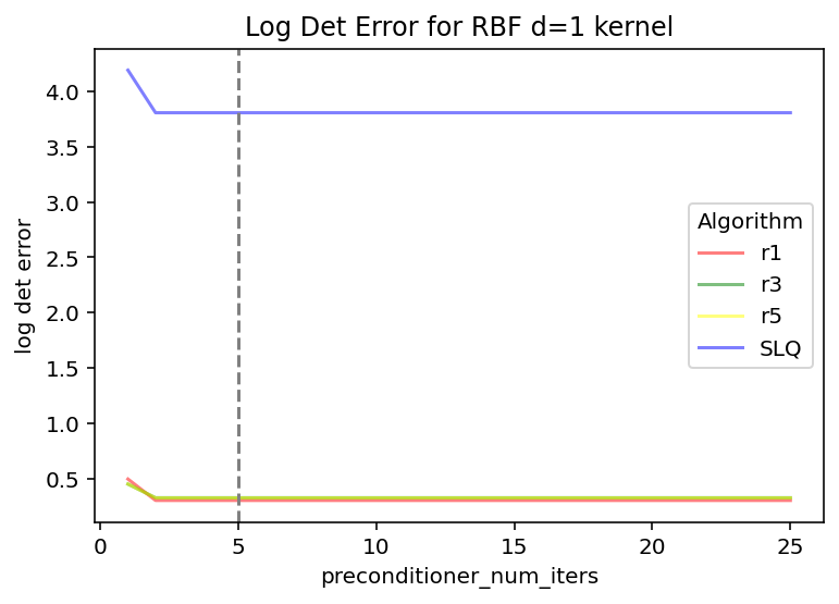
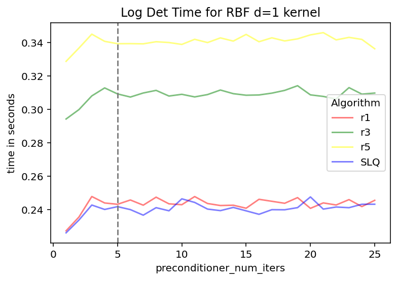
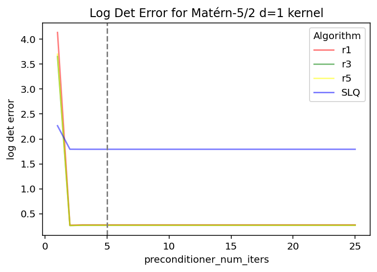
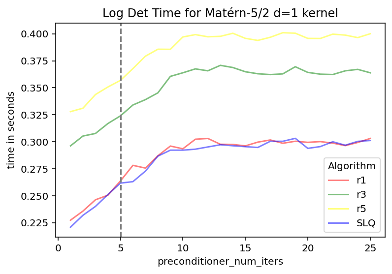
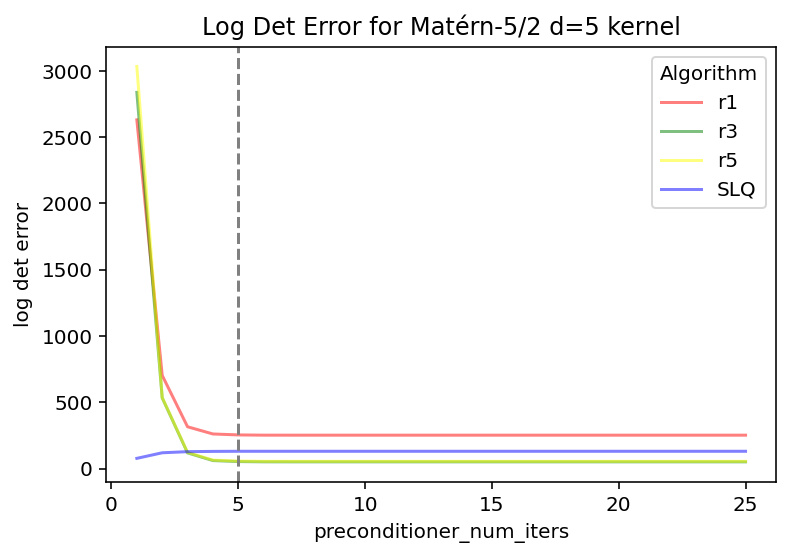
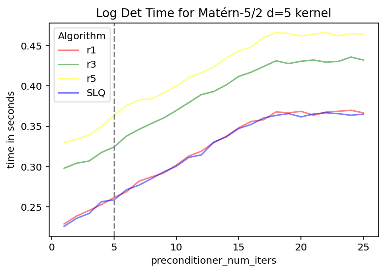
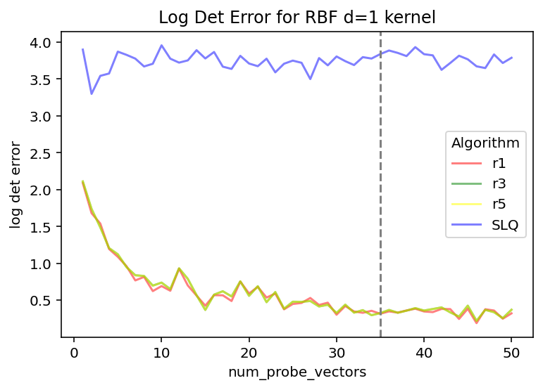
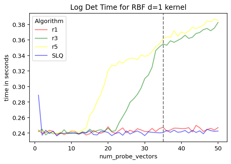
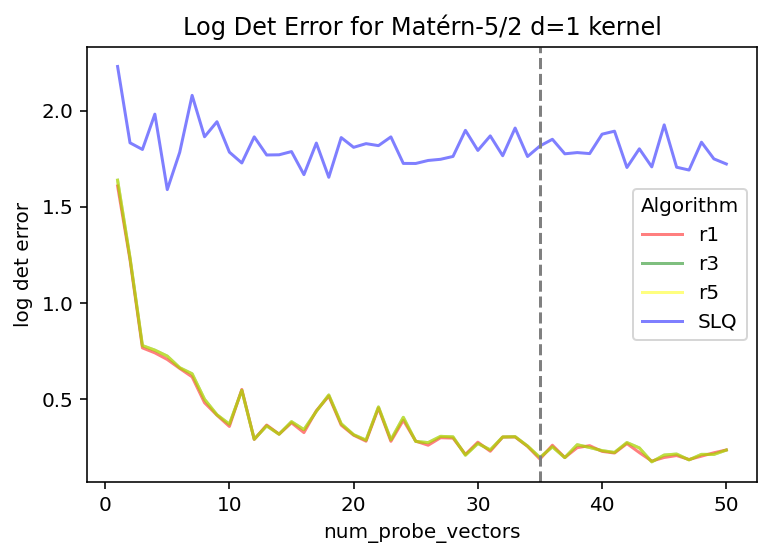
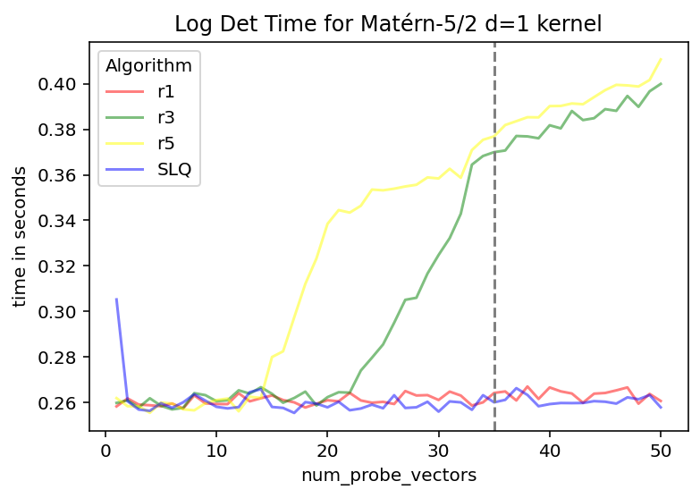
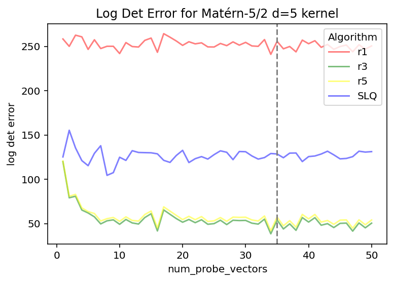
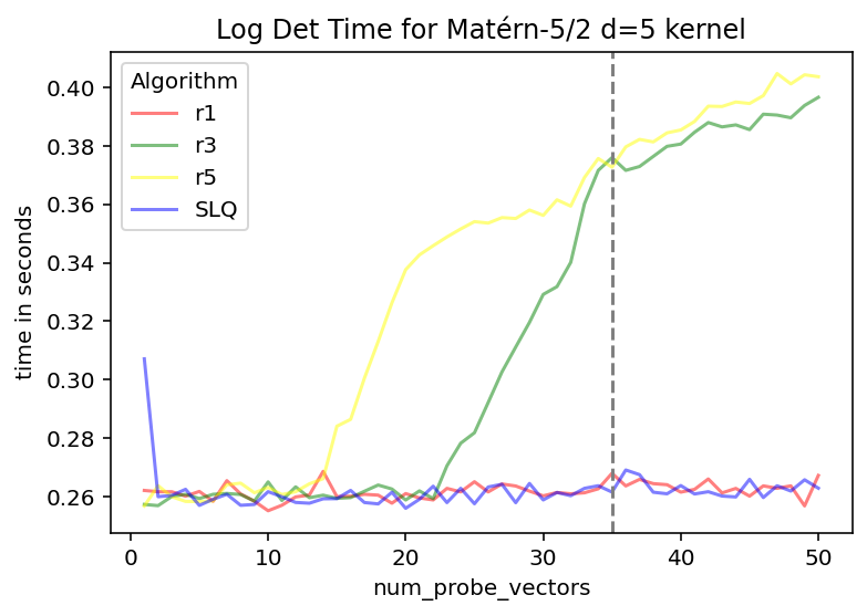
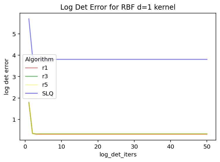
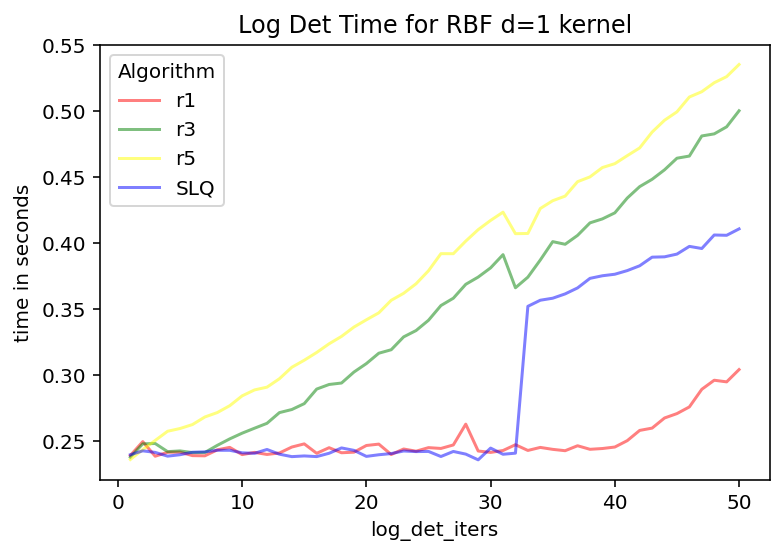
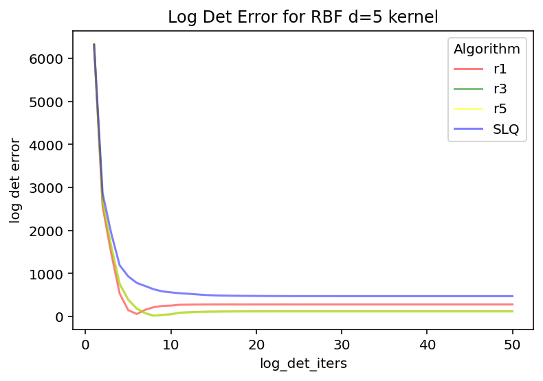
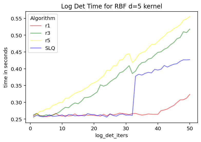
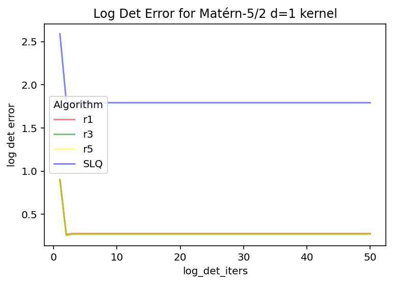
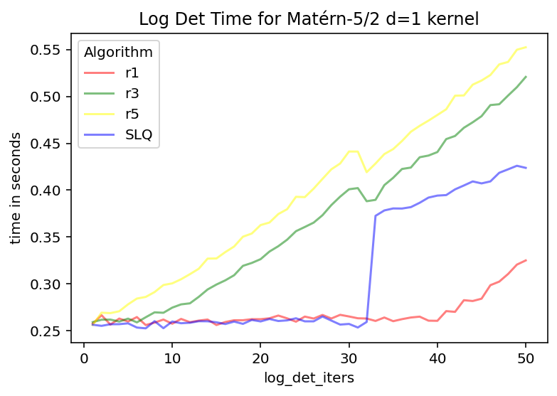
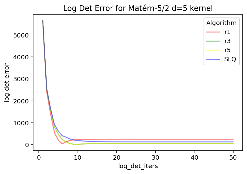
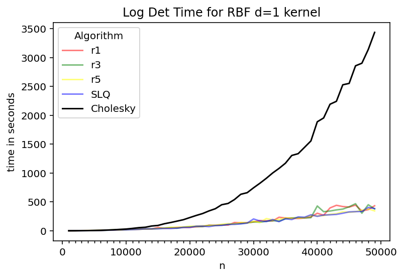
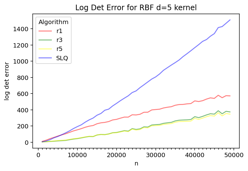
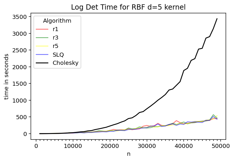
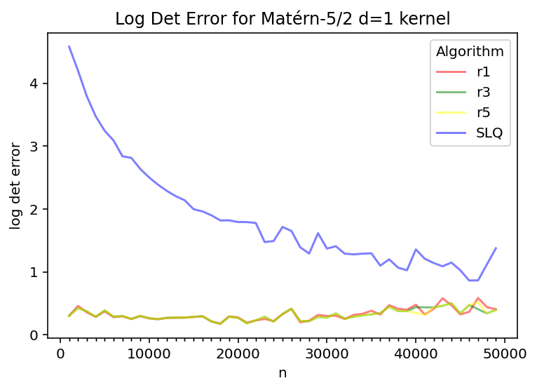
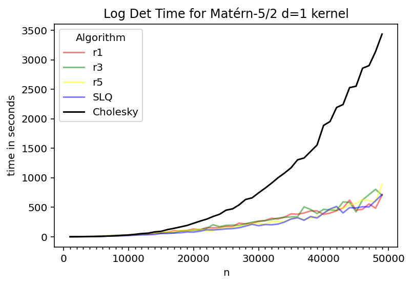
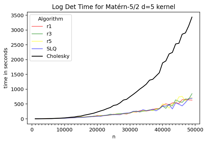
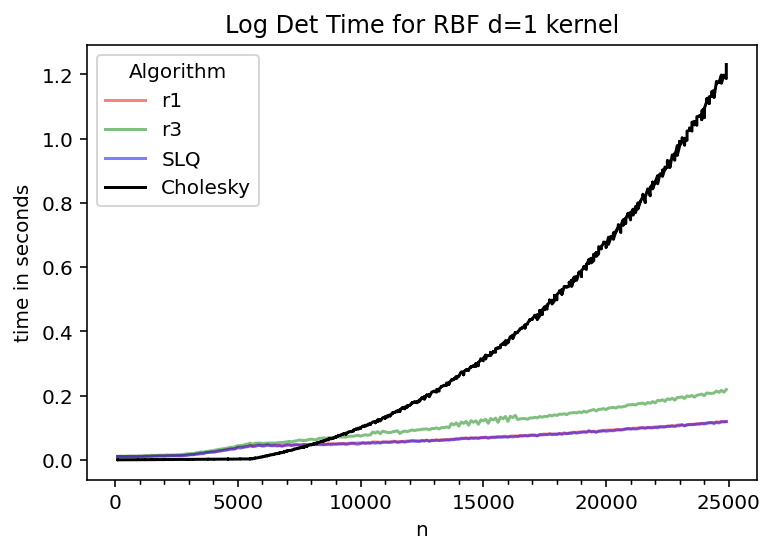
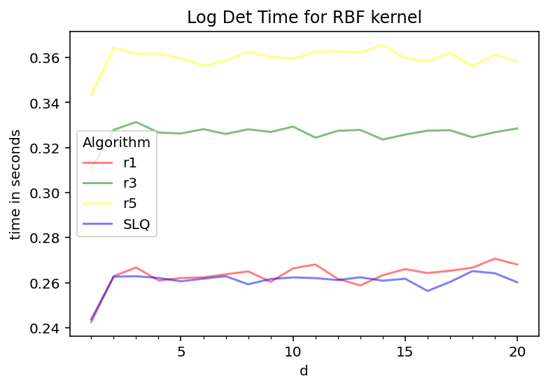
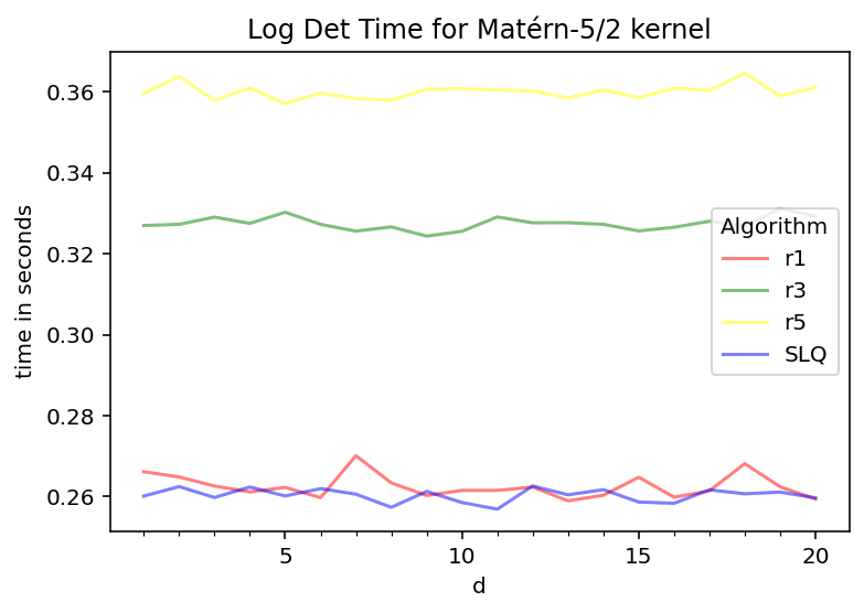
Using this implementation, we then measured the speed and accuracy of the r* and SLQ algorithms on the covariance matrices generated by the Matérn- and radial basis function (RBF) Gaussian process kernels [24]. Both kernels had their amplitude and length scale set to , and used index points sampled from a normal distribution. The graph of the measurements, as a function of the matrix’s size , are plotted in figures 2 through 5. The speeds include the time required to caculate the preconditioner, and the accuracies were measured as the absolute difference between the estimated log determinant and the log determinant as computed using a Cholesky decomposition. All computations were performed on Intel CPUs with 64-bit floats and the following parameter values:
-
•
Rademacher probe vectors,
-
•
iterations of the Lanczos algorithm in step 1 of Algorithm 1, and
-
•
A randomized, truncated SVD preconditioner using approximate eigenvalues computed using iterations.
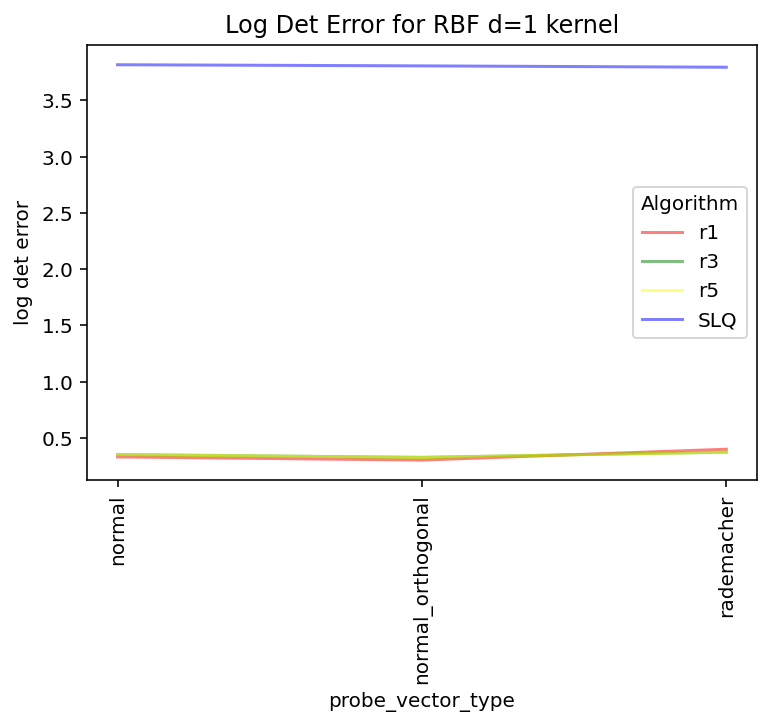
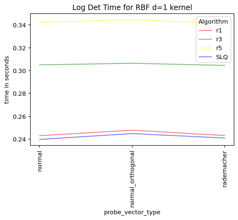
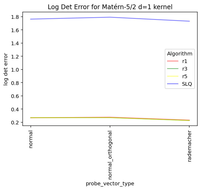
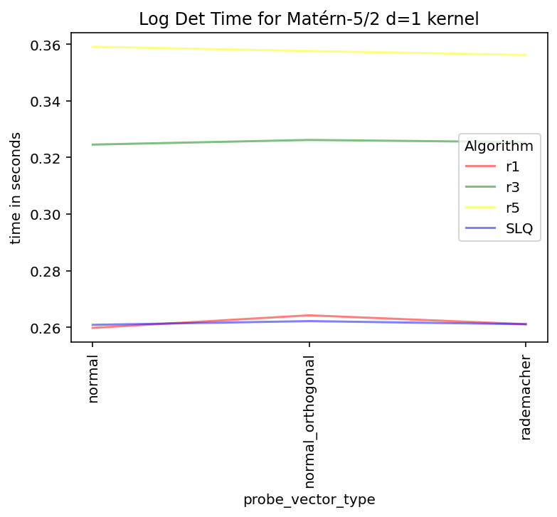
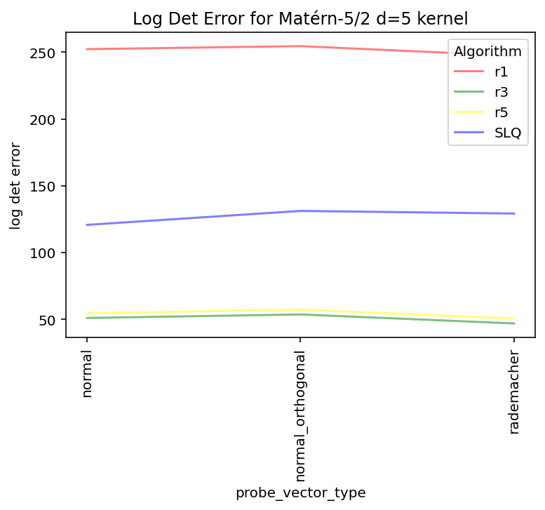
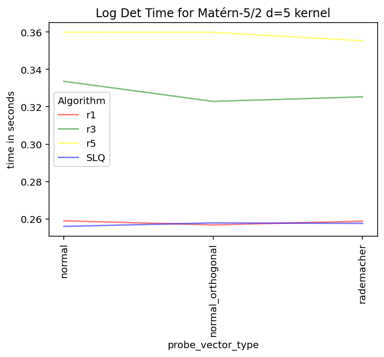
These parameters were selected to provide a reasonable speed/accuracy trade-off on two problem instances representative of our intended applications: the determinant of the covariance of Matérn- Gaussian process kernel in five dimensions with , and the derivative of that determinant. Graphs showing the sensitivity of each algorithm to each parameter (including the choice of probe vector type and preconditioner algorithm) can be found in the Appendix.
We also timed the algorithms on the NVidia A100 GPU [3]; these timings are shown in figures 6 through 9. The plots were again almost identical to those of and so were ommitted for clarity. (The error plots are also ommited because they are the same as when computed on the CPU.) It should also be noted that CUDA implementation of the Cholesky algorithm is currently faster (by a factor of over 100) on the older V100 and P100 GPUs than on the A100, despite the A100 being much faster in general.
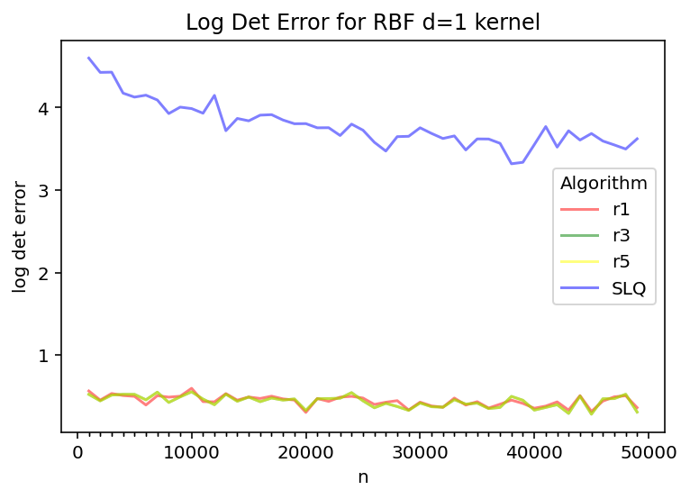
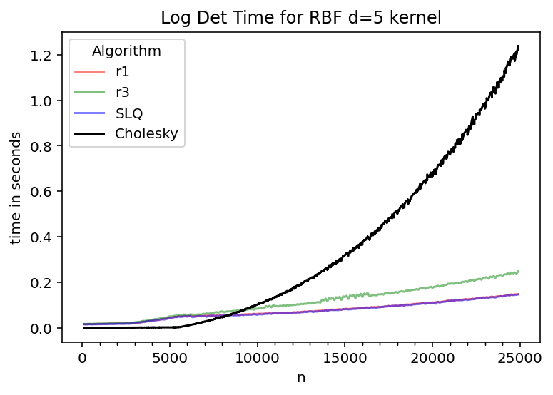
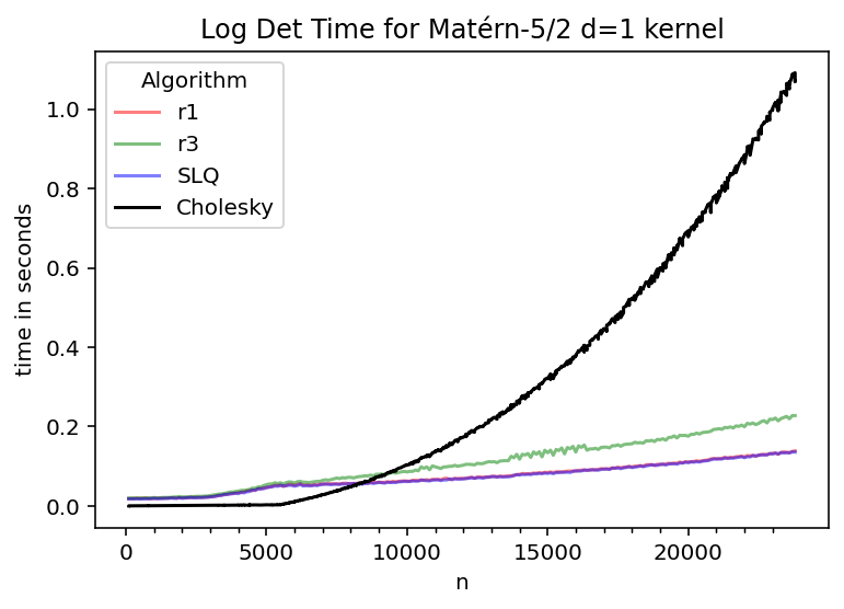
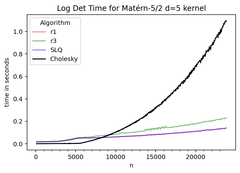
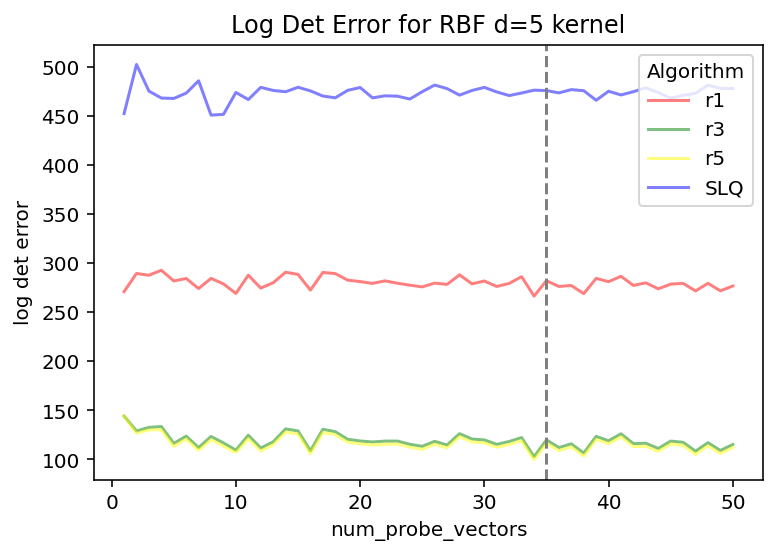
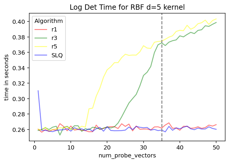
From these plots, we make the following observations:
-
•
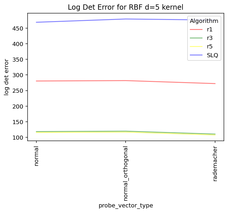
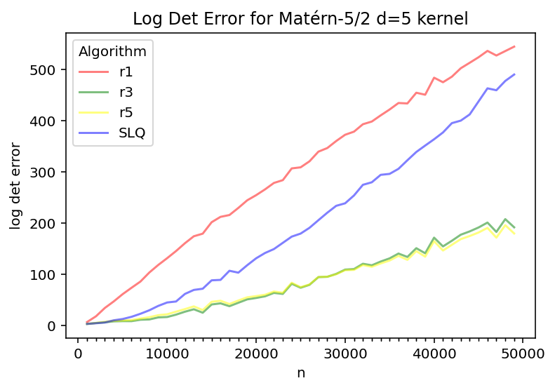
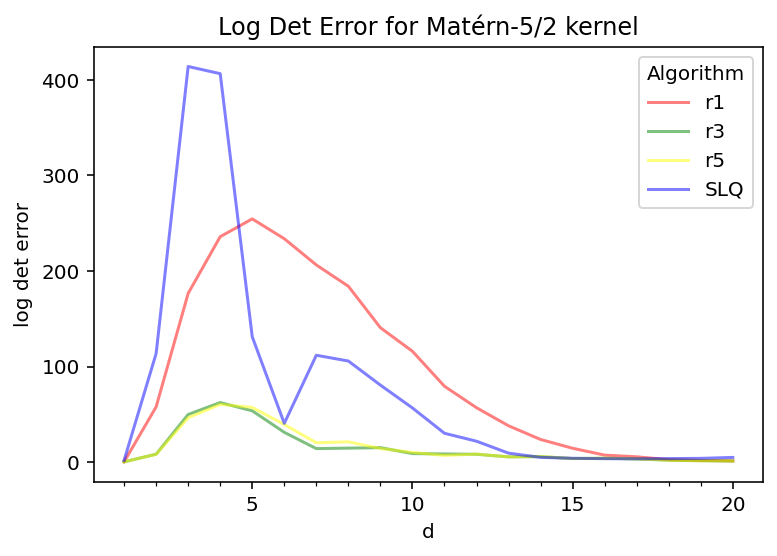
The r3 and r5 algorithms consistently have the lowest errors over the four kernel types and matrix sizes (up to 50,000) investigated. It is particularly noteworthy that r5 does not have a noticeably lower error than r3, despite being a closer approximation to in theory.
-
•
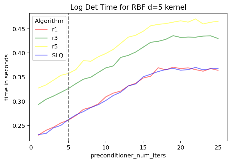
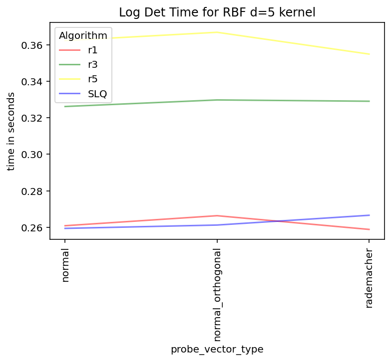
All of the r* and SLQ algorithms have approximately the same running time when measured on Intel CPUs. When measured on NVidia A100 GPUs, the r1 and SLQ algorithms have almost exactly the same running time and are slightly faster than the r3 algorithm.
-
•
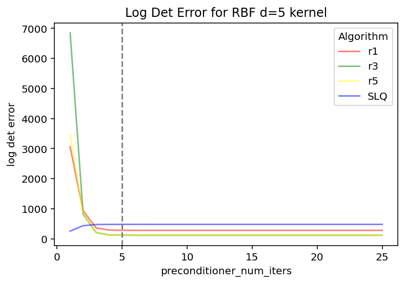
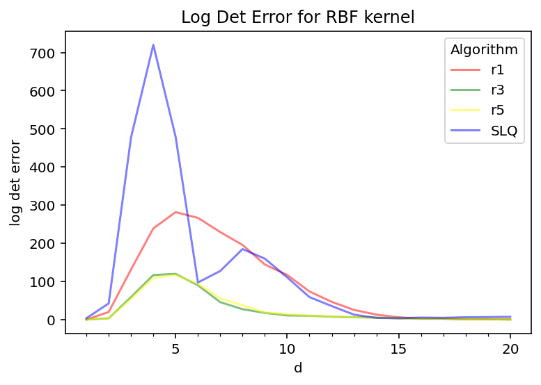
The underlying dimension ”d” of the Gaussian process has an extremely large impact on the accuracy of the approximation algorithms. For 50,000 by 50,000 matrices for example, the absolute errors of the r3 and r5 algorithms on the kernels are over 400 times that of their errors on the kernels.
To understand that last item more deeply, we ran a sweep over different ”d” values while holding the matrix size fixed at ; the results are presented in Figure 10. For both RBF and Matérn- kernels, absolute errors were highest for intermediate values of centered around and lowest for and . The more accurate r3 and r5 algorithms had shorter and narrower error peaks than the r1 and SLQ algorithms, with SLQ having the highest error peaks overall.
4 Conclusions
We have presented an algorithm for computing a new family of approximations to the matrix determinant. This algorithm combines classical rational function approximations to with well known techniques like Hutchinson’s trace estimator and the novel (in the space of determinant approximation algorithms) union of partial fraction decompositions and fast multi-shift solvers. In our results, one member of this family, r3, consistently achieved a lower error than the state of the art stochastic lanczos quadrature approximation, with only a slightly higher running time. The accuracy advantage of r3 over SLQ was particularly significant when measured on covariance matrices coming from Gaussian process kernels with underlying dimension greater than one.
It would be interesting for future work to examine whether these patterns hold over a wider class of matrix families. We are also curious as to why for all of the examined algorithms it appears harder to approximate the determinant of a covariance matrix derived from points in the moderate underlying dimension ”d” range of to than it is for the or cases (Figure 10). Based on Figure 13, it appears that the preconditioner behaves oddly in those dimensions, with the error first increasing as the preconditioner size increases, and then decreasing more slowly than the theoretical work of [23] would suggest.
5 Bibliography
References
- [1] Christos Boutsidis, Petros Drineas, Prabhanjan Kambadur, Eugenia-Maria Kontopoulou, and Anastasios Zouzias. A randomized algorithm for approximating the log determinant of a symmetric positive definite matrix. Linear Algebra and its Applications, 533:95–117, 2017.
- [2] James Bradbury, Roy Frostig, Peter Hawkins, Matthew James Johnson, Chris Leary, Dougal Maclaurin, George Necula, Adam Paszke, Jake VanderPlas, Skye Wanderman-Milne, and Qiao Zhang. JAX: composable transformations of Python+NumPy programs, 2018.
- [3] Jack Choquette, Wishwesh Gandhi, Olivier Giroux, Nick Stam, and Ronny Krashinsky. Nvidia a100 tensor core gpu: Performance and innovation. IEEE Micro, 41(2):29–35, 2021.
- [4] Joshua V Dillon, Ian Langmore, Dustin Tran, Eugene Brevdo, Srinivas Vasudevan, Dave Moore, Brian Patton, Alex Alemi, Matt Hoffman, and Rif A Saurous. Tensorflow distributions. arXiv preprint arXiv:1711.10604, 2017.
- [5] Mark Ebden. Gaussian processes: A quick introduction. arXiv preprint arXiv:1505.02965, 2015.
- [6] Ethan N. Epperly. Stochastic trace estimation. https://www.ethanepperly.com/index.php/2023/01/26/stochastic-trace-estimation/, 2023. Accessed 2024-04-17.
- [7] Joan Gimeno Alquézar. On computation of matrix logarithm times a vector. Master’s thesis, Universitat Politècnica de Catalunya, 2017.
- [8] Nathan Halko, Per-Gunnar Martinsson, and Joel A Tropp. Finding structure with randomness: Probabilistic algorithms for constructing approximate matrix decompositions. SIAM review, 53(2):217–288, 2011.
- [9] Insu Han, Dmitry Malioutov, and Jinwoo Shin. Large-scale log-determinant computation through stochastic chebyshev expansions. In International Conference on Machine Learning, pages 908–917. PMLR, 2015.
- [10] M.F. Hutchinson. A stochastic estimator of the trace of the influence matrix for laplacian smoothing splines. Communications in Statistics - Simulation and Computation, 19(2):433–450, 1990.
- [11] Beat Jegerlehner. Krylov space solvers for shifted linear systems. arXiv preprint hep-lat/9612014, 1996.
- [12] RP Kelisky and TJ Rivlin. A rational approximation to the logarithm. Mathematics of Computation, 22(101):128–136, 1968.
- [13] Andrew V Knyazev. Toward the optimal preconditioned eigensolver: Locally optimal block preconditioned conjugate gradient method. SIAM journal on scientific computing, 23(2):517–541, 2001.
- [14] Cornelius Lanczos. An iteration method for the solution of the eigenvalue problem of linear differential and integral operators. 1950.
- [15] Dean J Lee and Ilse CF Ipsen. Zone determinant expansions for nuclear lattice simulations. Physical review C, 68(6):064003, 2003.
- [16] Per-Gunnar Martinsson and Joel A Tropp. Randomized numerical linear algebra: Foundations and algorithms. Acta Numerica, 29:403–572, 2020.
- [17] R. Kelley Pace and James P. LeSage. Chebyshev approximation of log-determinants of spatial weight matrices. Computational Statistics & Data Analysis, 45(2):179–196, 2004.
- [18] Volker Strassen. Vermeidung von divisionen. Journal für die reine und angewandte Mathematik, 264:184–202, 1973.
- [19] Volker Strassen et al. Gaussian elimination is not optimal. Numerische mathematik, 13(4):354–356, 1969.
- [20] Llewellyn Hilleth Thomas. Elliptic problems in linear difference equations over a network. Watson Sci. Comput. Lab. Rept., Columbia University, New York, 1:71, 1949.
- [21] Shashanka Ubaru, Jie Chen, and Yousef Saad. Fast estimation of tr(f(a)) via stochastic lanczos quadrature. SIAM Journal on Matrix Analysis and Applications, 38(4):1075–1099, 2017.
- [22] Ke Wang, Geoff Pleiss, Jacob Gardner, Stephen Tyree, Kilian Q Weinberger, and Andrew Gordon Wilson. Exact gaussian processes on a million data points. Advances in neural information processing systems, 32, 2019.
- [23] Jonathan Wenger, Geoff Pleiss, Philipp Hennig, John Cunningham, and Jacob Gardner. Preconditioning for scalable gaussian process hyperparameter optimization. In International Conference on Machine Learning, pages 23751–23780. PMLR, 2022.
- [24] Christopher KI Williams and Carl Edward Rasmussen. Gaussian processes for machine learning, volume 2. MIT press Cambridge, MA, 2006.
- [25] Felix Xinnan X Yu, Ananda Theertha Suresh, Krzysztof M Choromanski, Daniel N Holtmann-Rice, and Sanjiv Kumar. Orthogonal random features. Advances in neural information processing systems, 29, 2016.
- [26] Yunong Zhang and William E Leithead. Approximate implementation of the logarithm of the matrix determinant in gaussian process regression. Journal of Statistical Computation and Simulation, 77(4):329–348, 2007.
6 Appendix
In this section, we investigate the sensitivity of our approximation algorithms to their hyperparameters.
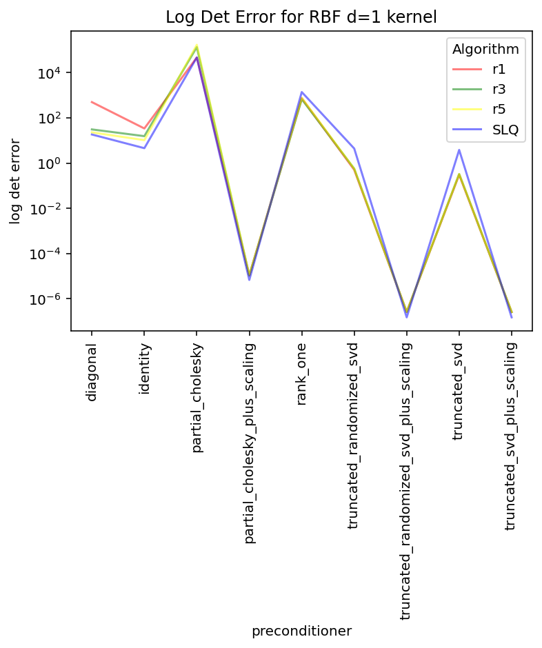
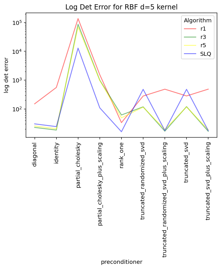
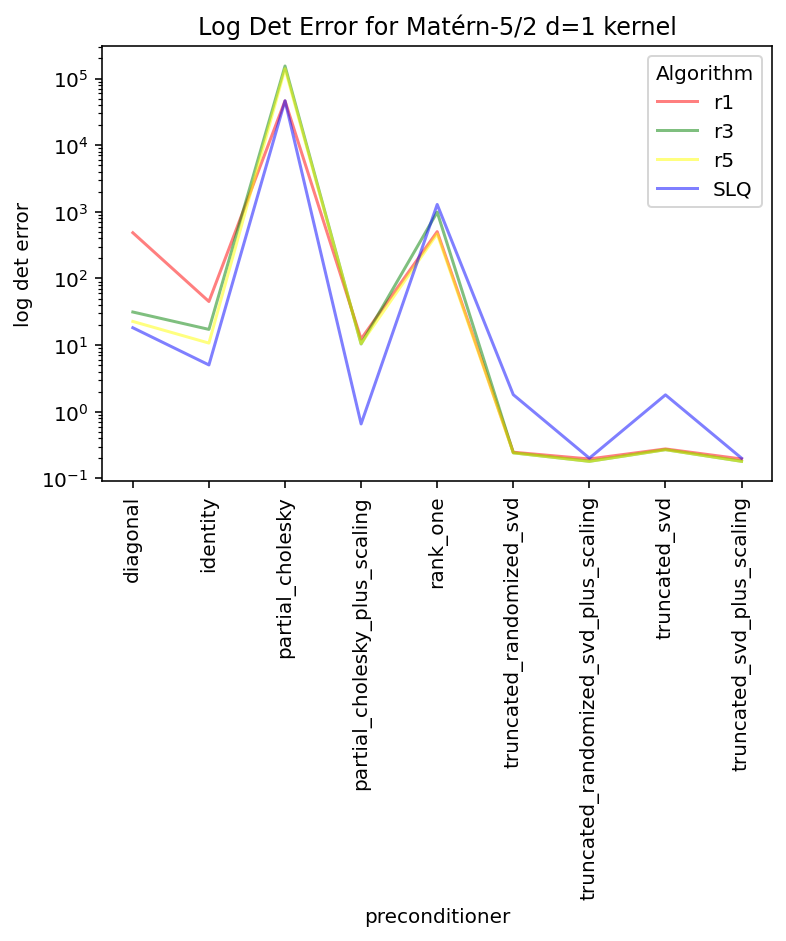
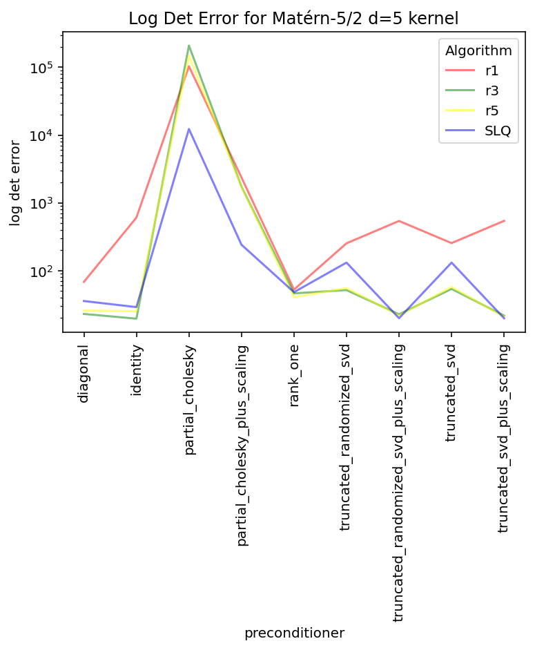
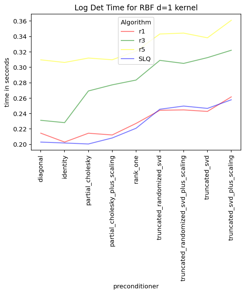
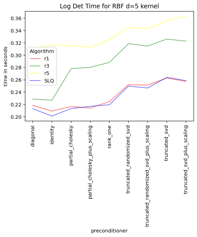
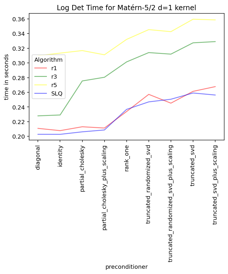
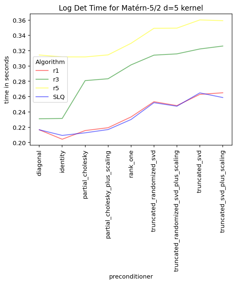
Figures 11 and 12 show their performance as a function of the preconditioner used. The preconditioners examined are
-
•
Identity: .
-
•
Diagonal: .
-
•
Rank One: where is ’s largest eigenvalue, is the corresponding eigenvector, and is a diagonal matrix .
-
•
Partial Cholesky: where is the incomplete Cholesky factorization of of rank and .
-
•
Partial Cholesky plus scaling: where is the incomplete Cholesky factorization of of rank and is the sum of the Gaussian process’s jitter and observation noise variance parameters.
-
•
Truncated SVD: where is the matrix formed by ’s top standard eigenvalues as computed by the Locally Optimal Block Preconditioned Conjugated Gradient algorithm [13] and implemented in jax.experimental.sparse.linalg.lobpcg_standard.
-
•
Truncated SVD plus scaling: Same as above, but with .
-
•
Truncated Randomized SVD: where is the approximate SVD described in [8].
-
•
Truncated Randomized SVD plus scaling: Same as above, but with .
The ’normal orthogonal’ probe vector type is an application of Orthogonal Monte Carlo [25]. These probe vectors are generated via the following process: , where is the variance of the Normal distribution (here ), is a diagonal matrix filled with i.i.d random variables sampled from a -distribution with degrees of freedom, and is a by random orthogonal matrix. As proven in [25], each column of is marginally distributed as a spherical multivariate normal. By sampling in this way, we can enforce orthogonality on the probe vectors, which can often be used to reduce variance.