V-line tensor tomography: numerical results

Abstract

This article presents the numerical verification and validation of several inversion algorithms for V-line transforms (VLTs) acting on symmetric 2-tensor fields in the plane. The analysis of these transforms and the theoretical foundation of their inversion methods were studied in a recent work [8]. We demonstrate the efficient recovery of an unknown symmetric 2-tensor field from various combinations of the longitudinal, transverse, and mixed VLTs, their corresponding first moments, and the star VLT. The paper examines the performance of the proposed algorithms in different settings and illustrates the results with numerical simulations on smooth and non-smooth phantoms.

Keywords: Inverse problems, V-line transform, broken ray transform, star transform, tensor tomography, numerical simulations, inversion algorithms, numerical solution of PDEs

Mathematics subject classification 2010: 44A12, 44A60, 44A30, 47G10, 65R10, 65R32

1 Introduction

Various generalizations of the Radon transform, involving integrals over piecewise linear trajectories, have been considered in recent years by different research groups. Some typical examples include operators mapping a scalar function to its integrals along broken rays/lines (also called “V-lines”) or over stars (finite unions of rays emanating from a common vertex). Such integral transforms appear in single scattering optical tomography [16, 19], single scattering X-ray tomography [26, 33], fluorescence imaging [18], Compton camera imaging [11, 12], Compton scattering emission tomography with collimated receivers [27, 32], and gamma ray transmission/emission imaging [29]. A detailed discussion of the history and the state of the art of these generalized Radon transforms, as well as their applications in various imaging modalities can be found in the recent book [3].

From the mathematical point of view, the broken ray/V-line transforms and their generalizations can be split into two distinct groups: those with the vertices of integration submanifolds inside the support of the integrand, and those where the vertices are outside (or on the boundary) of the support. This paper deals with transforms of the first type, and we briefly review below the relevant results on the subject. Several VLTs defined through a rotation invariant family of V-lines were studied in [1, 9, 10, 31], where the authors came up with various inversion formulas of the transforms, as well as implemented and analyzed the performance of the resulting numerical algorithms. VLTs using translation invariant families of V-lines were studied in [4, 17, 21, 25, 26, 31]. The obtained results included different inversion formulas, their numerical verification and validation, range description of the transforms, and support theorems. VLTs arising in imaging models using curvilinear detectors (corresponding to V-lines with focused rays) have been analyzed in [25, 26, 31]. Microlocal analysis of VLTs has been discussed in [2, 31]. The study of various properties and the inversion of the star transform has been conducted in [5, 34]. Several extensions of the VLT to three and higher dimensions (the conical Radon transforms) have been studied in [4, 20, 21, 28]. The V-line transform has also been generalized to more general objects, such as vector and tensor fields in $\mathbb{R}^{2}$. In [6], the authors introduced a new set of generalized V-line transforms (longitudinal, transverse, and their first integral moments), studied their properties, and derived various inversion algorithms to recover a vector field in $\mathbb{R}^{2}$ from different combinations of those transforms. The numerical verification and validation of the inversion methods proposed in [6] were demonstrated in the follow-up article [7]. Motivated by [1, 6, 9], the authors of [13] studied rotationally invariant V-line transforms of vector fields and came up with two approaches for recovering the unknown vector field supported in a disk.

Another class of integral transforms considered in the literature is concerned with broken rays reflecting from the boundary of an obstacle (sometimes known as a reflector). In [23], the authors studied this problem for scalar fields on a Riemannian surface in the presence of a strictly convex obstacle. Later, this work was extended to symmetric $m$-tensor fields in a similar setting in [22]. The broken ray transform of two tensors arises from the linearization of the length function of broken rays [23] and can be used in the field of seismic imaging. Notably, in this setting authors showed that the kernel of the longitudinal transform consists of all potential tensor fields, which is aligned with the theory of straight-line transforms. In a recent work [24], the authors considered a similar setup and proved uniqueness results for the broken ray transform acting on a combination of functions and vector fields on surfaces.

As a natural extension of works [6, 7], we studied the V-line transforms of symmetric 2-tensor fields in $\mathbb{R}^{2}$ and discovered multiple interesting results about those operators [8]. In particular, it was shown that the kernel descriptions of the longitudinal and transverse V-line transforms are very different from their counterparts appearing in the theory of straight-line transforms. We obtained exact inversion formulas to reconstruct a symmetric 2-tensor field from various combinations of longitudinal, transverse, and mixed V-line transforms and their first integral moments. We also derived an inversion formula for the star transform of symmetric 2-tensor fields. In this paper, our aim is to verify and validate all inversion algorithms arising from the theoretical discoveries of [8], and analyze their performance on various phantoms. All our simulations are done in MATLAB. To show the robustness of our numerical algorithms, we have done the reconstructions in the presence of various levels of noise.

The rest of the article is organized as follows. In Section 2, we introduce the integral transforms of interest and the required notations that we use throughout this article. At the end of that section, we present two tables (Tables 1, 2) that provide a summary of the algorithms studied in the paper, and shortcuts to the appropriate sections discussing the reconstructions from particular combinations of the transforms. Section 3 starts with a description of phantoms we used for numerical simulations and discusses the details of generating the forward data. A discussion about numerical solutions of certain PDEs required in some of our algorithms is presented at the end of that section. All numerical simulations and image reconstructions are demonstrated in Section 4. This section is divided into subsections, each of which focuses on a specific combination of transforms used for the reconstruction of the tensor fields (for details, see Tables 1, 2). We conclude the article with acknowledgments in Section 5.

2 Definitions and notations

This section is devoted to introducing the notations and definitions used throughout this article. The bold font letters are used to denote vectors and 2-tensors in $\mathbb{R}^{2}$ (e.g., x, u, v, f, etc.), and the regular font letters are used to denote scalars (e.g. $x_{i}$, $h$, $f_{ij}$, etc). The space of symmetric $2$-tensor fields defined on some ball $D\subset\mathbb{R}^{2}$ is denoted by $S^{2}(D)$ and the space of twice differentiable compactly supported tensor fields is denoted by $C_{c}^{2}\left(S^{2};D\right)$. The inner product in $S^{2}(D)$ is given by

$$\langle\textbf{{f}},\textbf{{g}}\rangle=\sum_{i,j=1}^{2}f_{ij}g_{ij}=f_{11}g_{11}+2f_{12}g_{12}+f_{22}g_{22}.$$ (1)

Next, we recall various well-known differential operators on scalar functions, vector fields, and tensor fields, which are needed in the upcoming discussions. For a scalar function $\varphi(x_{1},x_{2})$ and a vector field $\textbf{{f}}=(f_{1},f_{2})$, we define the notations

$$\mathrm{d}\varphi=\left(\frac{\partial\varphi}{\partial x_{1}},\frac{\partial\varphi}{\partial x_{2}}\right),\ \ \mathrm{d}^{\perp}\varphi=\left(-\frac{\partial\varphi}{\partial x_{2}},\frac{\partial\varphi}{\partial x_{1}}\right),\ \ \delta\textbf{{f}}=\frac{\partial f_{1}}{\partial x_{1}}+\frac{\partial f_{2}}{\partial x_{2}},\ \ \delta^{\perp}\textbf{{f}}=\frac{\partial f_{2}}{\partial x_{1}}-\frac{\partial f_{1}}{\partial x_{2}}.$$ (2)

These operators are naturally generalized to higher-order tensor fields in the following way:

• For a vector field f:

  $$(\mathrm{d}\textbf{{f}})_{ij}=\frac{1}{2}\left(\frac{\partial f_{i}}{\partial x_{j}}+\frac{\partial f_{j}}{\partial x_{i}}\right)\quad\mbox{and}\quad(\mathrm{d}^{\perp}\textbf{{f}})_{ij}=\frac{1}{2}\left((-1)^{j}\frac{\partial f_{i}}{\partial x_{3-j}}+(-1)^{i}\frac{\partial f_{j}}{\partial x_{3-i}}\right).$$

• For a symmetric 2-tensor field f:

  $$(\delta\textbf{{f}})_{i}=\frac{f_{i1}}{\partial x_{1}}+\frac{f_{i2}}{\partial x_{2}}=\frac{f_{ij}}{\partial x_{j}}\quad\mbox{and}\quad(\delta^{\perp}\textbf{{f}})_{i}=-\frac{f_{i1}}{\partial x_{2}}+\frac{f_{i2}}{\partial x_{1}}=(-1)^{j}\frac{f_{ij}}{\partial x_{3-j}}.$$

The directional derivative of a function $h$ in the direction $\textbf{{u}}\in\mathbb{S}^{1}$ is denoted by $D_{\textbf{{u}}}$, i.e.

$$D_{\textbf{{u}}}h=\textbf{{u}}\cdot\mathrm{d}h.$$ (3)

Remark 1.

For a detailed discussion of these operators, $\mathrm{d}$, $\mathrm{d}^{\perp}$, $\delta$, and $\delta^{\perp}$, we refer [14, 30].

For two fixed linearly independent unit vectors u and v, the rays emanating from $\textbf{{x}}\in\mathbb{R}^{2}$ in directions u and v are given by

$$L_{\textbf{{u}}}(\textbf{{x}})=\left\{\textbf{{x}}+t\textbf{{u}}:0\leq t<\infty\right\}\quad\mbox{ and }\quad L_{\textbf{{v}}}(\textbf{{x}})=\left\{\textbf{{x}}+t\textbf{{v}}:0\leq t<\infty\right\}.$$

A V-line with the vertex x is the union of rays $L_{\textbf{{u}}}(\textbf{{x}})$ and $L_{\textbf{{v}}}(\textbf{{x}})$. We work with data given on the space V-lines that have fixed ray directions $(\textbf{{u}}\ \&\ \textbf{{v}})$, and this space is parametrized simply by the vertex x. Now, we are ready to recall the definitions of the transforms of our interest. These transforms are introduced in [8], where authors present various inversion algorithms to recover a symmetric $2$-tensor field with different combinations of introduced transforms.

Definition 1.

1. The divergent beam transform $\mathcal{X}_{\textbf{{u}}}$ of function $h$ at $\textbf{{x}}\in\mathbb{R}^{2}$ in the direction $\textbf{{u}}\in\mathbb{S}^{1}$ is defined as:

   $$\mathcal{X}_{\textbf{{u}}}h(\textbf{{x}})=\int_{0}^{\infty}h(\textbf{{x}}+t\textbf{{u}})\,dt.$$ (4)

2. The $1^{st}$ moment divergent beam transform of a function $h$ in the direction $\textbf{{u}}\in\mathbb{S}^{1}$ is defined as follows

   $$\mathcal{X}^{1}_{\textbf{{u}}}h=\int_{0}^{\infty}h(\textbf{{x}}+t\textbf{{u}})\,t\,dt.$$ (5)

3. The V-line transform of a function $h$ with branches in the directions $\textbf{{u}},\ \textbf{{v}}\in\mathbb{S}^{1}$ is defined as follows

   $$\mathcal{V}h(\textbf{{x}})=\mathcal{X}_{\textbf{{u}}}h(\textbf{{x}})+\mathcal{X}_{\textbf{{v}}}h(\textbf{{x}}).$$ (6)

Definition 2.

For two vectors $\textbf{{u}}=(u_{1},u_{2})$ and $\textbf{{v}}=(v_{1},v_{2})$, the tensor product $\textbf{{u}}\otimes\textbf{{v}}$ is a rank-2 tensor with its $ij$-th component defined by

$$(\textbf{{u}}\otimes\textbf{{v}})_{ij}=u_{i}v_{j}.$$ (7)

The symmetrized tensor product $\textbf{{u}}\odot\textbf{{v}}$ is then defined as

$$\textbf{{u}}\odot\textbf{{v}}=\frac{1}{2}\left(\textbf{{u}}\otimes\textbf{{v}}+\textbf{{v}}\otimes\textbf{{u}}\right).$$ (8)

We use the notation $\textbf{{u}}^{2}$ for the tensor (symmetrized) product of a vector u with itself, that is,

$$\textbf{{u}}^{2}=\textbf{{u}}\odot\textbf{{u}}=\textbf{{u}}\otimes\textbf{{u}}.$$

Definition 3.

Let $\textbf{{f}}\in C_{c}^{2}\left(S^{2};\mathbb{R}^{2}\right)$.

1. The longitudinal V-line transform of f is defined as

   $$\mathcal{L}_{\textbf{{u}},\textbf{{v}}}\,\textbf{{f}}\ =\mathcal{X}_{\textbf{{u}}}\left(\left\langle\textbf{{f}},\textbf{{u}}^{2}\right\rangle\right)+\mathcal{X}_{\textbf{{v}}}\left(\left\langle\textbf{{f}},\textbf{{v}}^{2}\right\rangle\right).$$ (9)

2. The transverse V-line transform of f is defined as

   $$\mathcal{T}_{\textbf{{u}},\textbf{{v}}}\,\textbf{{f}}\ =\mathcal{X}_{\textbf{{u}}}\left(\left\langle\textbf{{f}},(\textbf{{u}}^{\perp})^{2}\right\rangle\right)+\mathcal{X}_{\textbf{{v}}}\left(\left\langle\textbf{{f}},(\textbf{{v}}^{\perp})^{2}\right\rangle\right).$$ (10)

   Here $\textbf{{u}}^{\perp}=(u_{1},u_{2})^{\perp}=(-u_{2},u_{1})$ is the the normal vector to u.

3. The mixed V-line transform of f is defined as

   $$\mathcal{M}_{\textbf{{u}},\textbf{{v}}}\,\textbf{{f}}\ =\mathcal{X}_{\textbf{{u}}}\left(\left\langle\textbf{{f}},\textbf{{u}}\odot\textbf{{u}}^{\perp}\right\rangle\right)+\mathcal{X}_{\textbf{{v}}}\left(\left\langle\textbf{{f}},\textbf{{v}}\odot\textbf{{v}}^{\perp}\right\rangle\right).$$ (11)

4. The $1^{st}$ moment longitudinal V-line transform of f is defined as

   $$\mathcal{L}^{1}_{\textbf{{u}},\textbf{{v}}}\,\textbf{{f}}\ =\mathcal{X}^{1}_{\textbf{{u}}}\left(\left\langle\textbf{{f}},\textbf{{u}}^{2}\right\rangle\right)+\mathcal{X}^{1}_{\textbf{{v}}}\left(\left\langle\textbf{{f}},\textbf{{v}}^{2}\right\rangle\right).$$ (12)

5. The $1^{st}$ moment transverse V-line transform of f is defined as

   $$\mathcal{T}^{1}_{\textbf{{u}},\textbf{{v}}}\,\textbf{{f}}\ =\mathcal{X}^{1}_{\textbf{{u}}}\left(\left\langle\textbf{{f}},(\textbf{{u}}^{\perp})^{2}\right\rangle\right)+\mathcal{X}^{1}_{\textbf{{v}}}\left(\left\langle\textbf{{f}},(\textbf{{v}}^{\perp})^{2}\right\rangle\right).$$ (13)

6. The $1^{st}$ moment mixed V-line transform of f is defined as

   $$\mathcal{M}^{1}_{\textbf{{u}},\textbf{{v}}}\,\textbf{{f}}\ =\mathcal{X}^{1}_{\textbf{{u}}}\left(\left\langle\textbf{{f}},\textbf{{u}}\odot\textbf{{u}}^{\perp}\right\rangle\right)+\mathcal{X}^{1}_{\textbf{{v}}}\left(\left\langle\textbf{{f}},\textbf{{v}}\odot\textbf{{v}}^{\perp}\right\rangle\right).$$ (14)

Remark 2.

To simplify various calculations, we assume $\textbf{{u}}=(u_{1},u_{2})$ and $\textbf{{v}}=(-u_{1},u_{2})$, that is, the V-lines are symmetric with respect to the $y$-axis. This choice does not change the analysis of the general case since the data obtained in one setup of u and v can be transformed into the data obtained for the other setup and vice versa.

Next, we introduce another transform of interest known as the star transform. Unlike V-line transforms, star transform consists of multiple branches. In the upcoming definition, we identify a symmetric 2-tensor $\textbf{{f}}=\left(f_{ij}\right)$ with the vector $\textbf{{f}}=\left(f_{11},f_{12},f_{22}\right)\in\mathbb{R}^{3}$. In the same way the tensors $\textbf{{u}}^{2}$ and $\textbf{{u}}\odot\textbf{{v}}$ are identified with the vectors $\left(u_{1}^{2},u_{1}u_{2},u_{2}^{2}\right)$ and $\left(u_{1}v_{1},\frac{1}{2}(u_{1}v_{2}+u_{2}v_{1}),u_{2}v_{2}\right)$. Now, we are ready to define the star transform of a symmetric 2-tensor field.

Definition 4.

Let $\textbf{{f}}\in C_{c}^{2}\left(S^{2};\mathbb{R}^{2}\right)$, and let $\boldsymbol{\gamma}_{1},\boldsymbol{\gamma}_{2},\dots,\boldsymbol{\gamma}_{m}$ be distinct unit vectors in $\mathbb{R}^{2}$. The star transform of f is defined as

$$\mathcal{S}\textbf{{f}} =\sum_{i=1}^{m}c_{i}{\mathcal{X}}_{{\boldsymbol{\gamma}}_{i}}\begin{bmatrix}\textbf{{f}}\cdot{{\boldsymbol{\gamma}}_{i}}^{2}\\ \textbf{{f}}\cdot{{\boldsymbol{\gamma}}_{i}\odot{\boldsymbol{\gamma}}_{i}^{\perp}}\\ \textbf{{f}}\cdot({\boldsymbol{\gamma}}_{i}^{\perp})^{2}\end{bmatrix},$$ (15)

where $c_{1},c_{2},\dots,c_{m}$ are non-zero constants in $\mathbb{R}$.

In our theoretical work [8], we used specific combinations of these transforms and proved many inversion algorithms to recover a symmetric 2-tensor field in $\mathbb{R}^{2}$. Each inversion method will be discussed in upcoming sections, along with their implementations, to illustrate the effectiveness of the proposed algorithm. The tables below give the details of various combinations of the transforms considered in which section and the corresponding reconstruction results. The first table is concerned with the recovery of special kinds of symmetric 2-tensor fields, while the second table deals with the recovery of general symmetric 2-tensor fields.

Form of f	Combinations of transforms used to recover f	Sections and Figures
$\mathrm{d}^{2}\varphi$	$\mathcal{L}\textbf{{f}}$ or $\mathcal{M}\textbf{{f}}$ (formula (32))	4.1.1, Figure 2
$\mathrm{d}\mathrm{d}^{\perp}\varphi$	$\mathcal{L}\textbf{{f}}$ or $\mathcal{T}\textbf{{f}}$ or $\mathcal{M}\textbf{{f}}$ (formulas (34) and (35))	4.1.1, Figures 3, 4, 5
$\mathrm{d}\textbf{{g}}$ PH1	$\mathcal{L}\textbf{{f}}$ and $\mathcal{M}\textbf{{f}}$ (formulas (36), (37), (39), and (38))	4.1.2, Figures 6, 7, 8, 9
$\mathrm{d}\textbf{{g}}$ PH2	$\mathcal{L}\textbf{{f}}$ and $\mathcal{M}\textbf{{f}}$ (formulas (36), (37), (39), and (38))	4.1.2, Figures 10, 11, 12, 13

Table 1: Reconstruction of a special kind of symmetric 2-tensor field

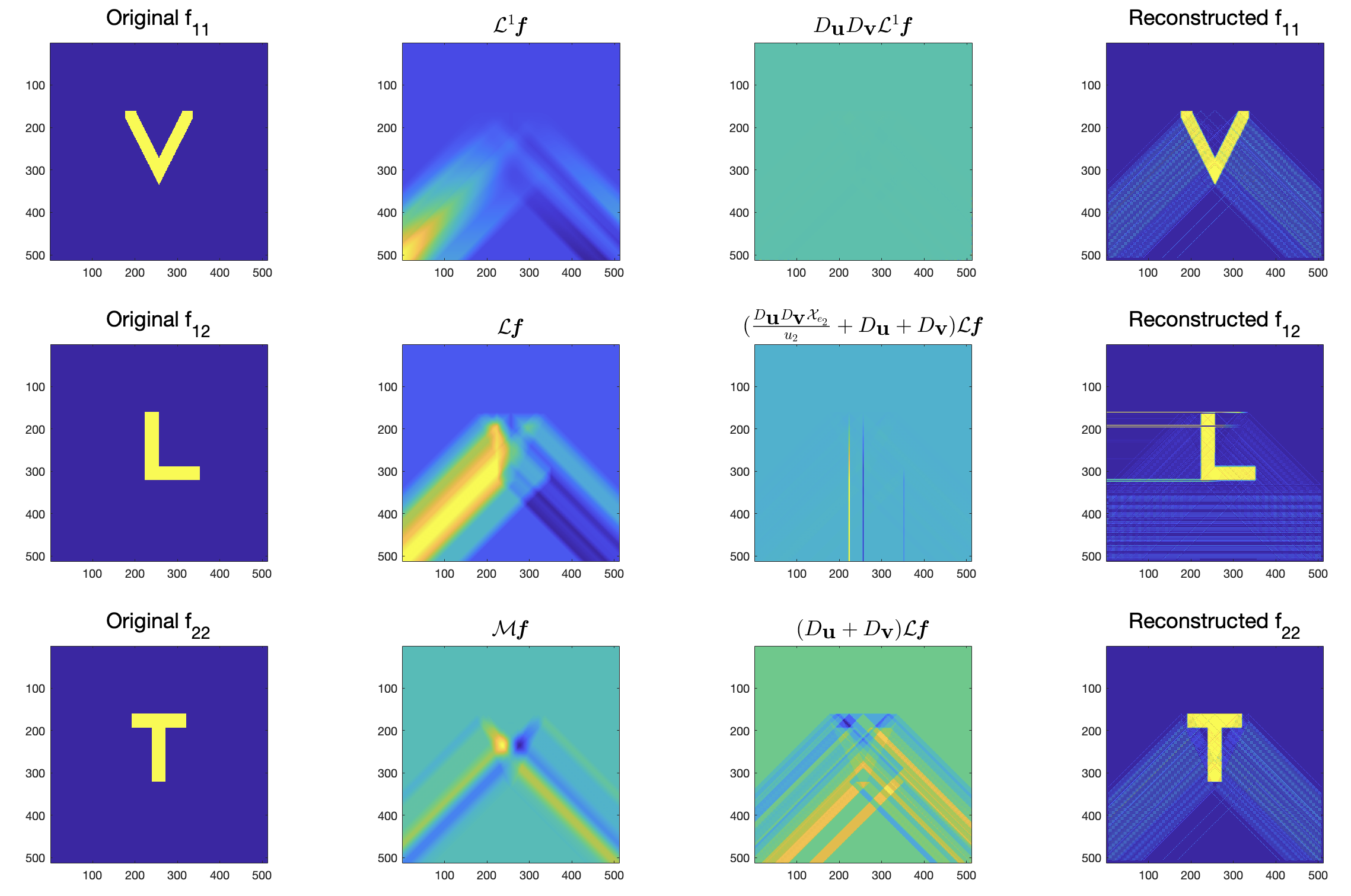
Figure 26: (Column-1) Components of f, (Column-2) first moment longitudinal ($\mathcal{L}^{1}\textbf{{f}}$), longitudinal ($\mathcal{L}\textbf{{f}}$) and mixed ($\mathcal{M}\textbf{{f}}$) V-line transforms of f, (Column-3) $D_{\textbf{{u}}}D_{\textbf{{v}}}\mathcal{L}^{1}\textbf{{f}}$, $\left(\frac{D_{\textbf{{u}}}D_{\textbf{{v}}}\mathcal{X}_{\textbf{{e}}_{2}}}{u_{2}}+D_{\textbf{{u}}}+D_{\textbf{{v}}}\right)\mathcal{L}\textbf{{f}}$ and $(D_{\textbf{{u}}}+D_{\textbf{{v}}})\mathcal{L}\textbf{{f}}$, (Column-4) reconstructed components of f when $\textbf{{u}}=(\cos{\pi/4},\sin{\pi/4})$ using formulas (53),(54),(55)

Combinations of transforms used to recover f	Sections and Figures
$\mathcal{L}\textbf{{f}}$, $\mathcal{T}\textbf{{f}}$, and $\mathcal{M}\textbf{{f}}$ ($u_{1}=u_{2}$) (formulas (42), (43), and (44))	4.2, Figures 14, 15
$\mathcal{L}\textbf{{f}}$, $\mathcal{T}\textbf{{f}}$, and $\mathcal{M}\textbf{{f}}$ ($u_{1}\neq u_{2}$) (formulas (47), (48), and (49))	4.2, Figures 16, 17, 18, 19
$\mathcal{L}\textbf{{f}}$, $\mathcal{L}^{1}\textbf{{f}}$, and $\mathcal{T}\textbf{{f}}$ ($u_{1}\neq u_{2}$) (formulas (50), (51), and (52))	4.3, Figures 20, 21, 22, 23
$\mathcal{L}\textbf{{f}}$, $\mathcal{L}^{1}\textbf{{f}}$, and $\mathcal{M}\textbf{{f}}$, (formulas (53), (54), and (55))	4.3, Figures 24, 25, 26, 27
$\mathcal{S}\textbf{{f}}$ (formula (57))	4.4, Figures 28, 29

Table 2: Full recovery of a general symmetric 2-tensor field

3 Phantoms and data formation

In this section, we introduce the phantoms that are used for our numerical experiments. Once the phantoms are defined, we present the steps to generate the forward data numerically, that is, the process of evaluating the transforms introduced in the above Section 2. In addition to these, we also discuss a method to find the solution to boundary value problems for partial differential equations, which is required in various inversion algorithms developed in [8].

3.1 Description of Phantoms

The performance of all inversion algorithms will be tested on the following two phantoms defined on $[-1,1]\times[-1,1]$. As we are dealing with symmetric $2$-tensor fields f in $\mathbb{R}^{2}$, each phantom has 3 components $f_{11}$, $f_{12}$, and $f_{22}$.

• Phantom 1: This is a smooth phantom, and the components $f_{11}$, $f_{12}$ $\&$ $f_{22}$ of f are different combinations of cutoff functions and are given by (see Figure 1)

  $$f_{11}(x,y)=F_{1}(x,y)+F_{2}(x,y)+F_{3}(x,y)+F_{4}(x,y)+F_{5}(x,y)+F_{6}(x,y)$$

  where

  $$F_{1}(x,y) =\begin{cases}e^{-0.05/(0.05-[x^{2}+y^{2}]},&x^{2}+y^{2}<0.05\\ 0,&x^{2}+y^{2}\geq 0.05\end{cases}$$

  $$F_{2}(x,y) =\begin{cases}e^{-0.03/(0.03-[(x-0.09)^{2}+(y-0.28)^{2}])},&(x-0.09)^{2}+(y-0.28)^{2}<0.03\\ 0,&(x-0.09)^{2}+(y-0.28)^{2}\geq 0.03\end{cases}$$

  $$F_{3}(x,y) =\begin{cases}e^{-0.03/(0.03-[(x+0.25)^{2}+(y-0.15)^{2}])},&(x+0.25)^{2}+(y-0.15)^{2}<0.03\\ 0,&(x+0.25)^{2}+(y-0.15)^{2}\geq 0.03\end{cases}$$

  $$F_{4}(x,y) =\begin{cases}e^{-0.03/(0.03-[(x+0.22)^{2}+(y+0.2)^{2}])},&(x+0.22)^{2}+(y+0.2)^{2}<0.03\\ 0,&(x+0.22)^{2}+(y+0.2)^{2}\geq 0.03\end{cases}$$

  $$F_{5}(x,y) =\begin{cases}e^{-0.03/(0.03-[(x-0.13)^{2}+(y+0.27)^{2}])},&(x+0.22)^{2}+(y+0.2)^{2}<0.03\\ 0,&(x+0.22)^{2}+(y+0.2)^{2}\geq 0.03\end{cases}$$

  $$F_{6}(x,y) =\begin{cases}e^{-0.03/(0.03-[(x-0.3)^{2}+y^{2}])},&(x-0.3)^{2}+y^{2}<0.03\\ 0,&(x-0.3)^{2}+y^{2}\geq 0.03.\end{cases}$$

  $$f_{12}(x,y)=G_{1}(x,y)+G_{2}(x,y)+G_{3}(x,y)\qquad\qquad\qquad\qquad\qquad\qquad\qquad\quad$$

  where

  $$G_{1}(x,y) =\begin{cases}e^{-0.1/\left(0.1-[x^{2}+y^{2}]\right)},&x^{2}+y^{2}<0.1\\ 0,&x^{2}+y^{2}\geq 0.1\end{cases}$$

  $$G_{2}(x,y) =\begin{cases}e^{-0.03/(0.03-[(x-0.3)^{2}+(y-0.2)^{2}])},&(x-0.3)^{2}+(y-0.2)^{2}<0.03\\ 0,&(x-0.3)^{2}+(y-0.2)^{2}\geq 0.03\end{cases}$$

  $$G_{3}(x,y) =\begin{cases}e^{-0.03/(0.03-[(x+0.3)^{2}+(y-0.2)^{2}])},&(x+0.3)^{2}+(y-0.2)^{2}<0.03\\ 0,&(x+0.3)^{2}+(y-0.2)^{2}\geq 0.03\end{cases}.$$

  And

  $$f_{22}(x,y)=H_{1}(x,y)+H_{2}(x,y)+H_{3}(x,y)+H_{4}(x,y)+H_{5}(x,y)\qquad\qquad$$

  with

  $$H_{1}(x,y) =\begin{cases}e^{-0.05/(0.05-[x^{2}+y^{2}]},&x^{2}+y^{2}<0.05\\ 0,&x^{2}+y^{2}\geq 0.05.\end{cases}$$

  $$H_{2}(x,y) =\begin{cases}e^{-0.03/(0.03-[x^{2}+(y-0.3)^{2}])},&x^{2}+(y-0.3)^{2}<0.03\\ 0,&x^{2}+(y-0.3)^{2}\geq 0.03\end{cases}$$

  $$H_{3}(x,y) =\begin{cases}e^{-0.03/(0.03-[x^{2}+(y+0.3)^{2}])},&x^{2}+(y+0.3)^{2}<0.03\\ 0,&x^{2}+(y+0.3)^{2}\geq 0.03\end{cases}$$

  $$H_{4}(x,y) =\begin{cases}e^{-0.03/(0.03-[(x+0.3)^{2}+y^{2}])},&(x+0.3)^{2}+y^{2}<0.03\\ 0,&(x+0.3)^{2}+y^{2}\geq 0.03\end{cases}$$

  $$H_{5}(x,y) =\begin{cases}e^{-0.03/(0.03-[(x-0.3)^{2}+y^{2}])},&(x-0.3)^{2}+y^{2}<0.03\\ 0,&(x-0.3)^{2}+y^{2}\geq 0.03\end{cases}.$$

• Phantom 2: This is a non-smooth case, the components $f_{11}$, $f_{12}$ $\&$ $f_{22}$ of f are taken to be “V”, “L”, and “T”, respectively (see Figure 1).

  $$f_{11}=\text{letter ``V"},\quad f_{12}=\text{letter ``L"},\quad f_{22}=\text{letter ``T"}.$$

Figure 1: The components of the phantoms considered in numerical reconstructions.

Remark 3.

We would like to mention here that some of our reconstruction algorithms work extremely well even for the non-smooth phantom, and hence, in those cases, we choose to show the reconstructions only for the non-smooth case to avoid repetition.

3.2 Data formation

For the numerical simulations comprising V-line transforms, we use the unit vectors $\textbf{{u}}=(\cos\phi,\sin\phi)$ (recall $\textbf{{v}}=(-\cos\phi,\sin\phi)$) with the choice of angles $\phi=\pi/3$, $\pi/4$, and $\pi/6$ depending on the inversion formula we are using. In the case of star transform, we work with three branches along $\phi_{1}=0$, $\phi_{2}=2\pi/3$, $\phi_{3}=4\pi/3$ with weights $c_{i}=1$ for $i=1,2,3.$

Since all the transforms introduced in Definitions 3 and 4 are linear combinations of divergent beam transform (4) and its first moments (5) of various projections of the unknown tensor field $\textbf{{f}}.$ To generate generalized V-line transforms and star transform of f, we need a method to numerically compute divergent beam transform and its first moment of a scalar field. The required algorithm has already been discussed in a recent work [7, Section 3.2], and we present this here briefly for the sake of completeness.

Numerical computation of the divergent beam transform and its first moment: Let $F$ be an $n\times n$ pixelized image $F$ defined on $[-1,1]\times[-1,1]$. Then, the divergent beam transform of $F$ is also of the size $n\times n$ since the rays are parametrized by vertices and the rays are emanating from the centers of pixels. Let $\textbf{{x}}=(x,y)$ be vertex and $\textbf{{u}}=(\cos\phi,\sin\phi)$ direction of the ray. The main step here is to find the intersections of the ray emanating from x in the direction u and the boundaries of square pixels appearing on the path of this ray. Next, we find the product of $F(i,j)$ and the length of the ray inside the pixel $(i,j)$, and by adding this product over all the pixels generates the divergent beam transform of $F$, $\mathcal{X}_{\textbf{{u}}}F(\textbf{{x}}).$

To evaluate the first moment of divergent beam transform of $F$, we need to consider the product of three quantities $F(i,j)$, the distance from the center of the pixel $(i,j)$, to the vertex x, and the length of the line segment of the ray inside the pixel $(i,j)$. Then, by adding this product over all the pixels, we get the required $\mathcal{X}^{1}_{\textbf{{u}}}F(\textbf{{x}}).$

As discussed above, to generate $\mathcal{L}\textbf{{f}},\mathcal{T}\textbf{{f}},$ and $\mathcal{M}\textbf{{f}}$ we evaluate the divergent beam transform $\mathcal{X}_{\textbf{{u}}}$ of the projections $\left\langle\textbf{{f}},\textbf{{u}}^{2}\right\rangle,\left\langle\textbf{{f}},(\textbf{{u}}^{\perp})^{2}\right\rangle,\left\langle\textbf{{f}},\textbf{{u}}\odot\textbf{{u}}^{\perp}\right\rangle$ and $\mathcal{X}_{\textbf{{v}}}$ of $\left\langle\textbf{{f}},\textbf{{v}}^{2}\right\rangle,\left\langle\textbf{{f}},(\textbf{{v}}^{\perp})^{2}\right\rangle,\left\langle\textbf{{f}},\textbf{{v}}\odot\textbf{{v}}^{\perp}\right\rangle$, and combine them according to the equations (9) (10), and (11). In a similar way, $\mathcal{L}^{1}\textbf{{f}},\mathcal{T}^{1}\textbf{{f}},$ and $\mathcal{M}^{1}\textbf{{f}},$ are generated by considering $\mathcal{X}^{1}_{\textbf{{u}}}$, $\mathcal{X}^{1}_{\textbf{{v}}}$ of the appropriate projections and combine them using formulas (12), (13), and (14). Finally, to generate $\mathcal{S}\textbf{{f}}$, we consider the divergent beam transform $\mathcal{X}_{\boldsymbol{\gamma}_{i}}$ of $\textbf{{f}}\cdot{{\boldsymbol{\gamma}}_{i}}^{2}$, $\textbf{{f}}\cdot{{\boldsymbol{\gamma}}_{i}\odot{\boldsymbol{\gamma}}_{i}^{\perp}}$, $\textbf{{f}}\cdot({\boldsymbol{\gamma}}_{i}^{\perp})^{2}$ for $i=1,2\dots m$ and use the formula (15) to combine them.

Another operator that is used repeatedly throughout the article is the directional derivative of a scalar function $h$ along u or v. Numerically $D_{\textbf{{u}}}h$ is computed in the following two steps ($D_{\textbf{{v}}}h$ is computed in exactly the same way):

• Calculate the gradient $\left(\partial_{x}h,\partial_{y}h\right)$ by Matlab function gradient

• Compute $\displaystyle D_{\textbf{{u}}}h=u_{1}\partial_{x}h+u_{2}\partial_{y}h.$

Remark 4.

For some inversion formulas in our theoretical paper [8], we need to solve boundary/initial value problems for partial differential equations (PDE), which requires an inversion of an $n^{2}\times n^{2}$ matrix. In all such experiments, we use images with a resolution of $160\times 160$ pixels to reduce the computational time. For all other experiments, we use images with a resolution of $512\times 512$ pixels.

3.3 Solving PDEs numerically

As mentioned above in Remark 4 that in some cases [8, Theorems 4, 5, and 6], the recovery of the unknown symmetric $2$-tensor field is achieved by solving boundary/initial value problems for PDEs. The partial differential equation that we encountered in [8, Theorems 4, 5, and 6] is of the following form:

$$a\partial_{x_{1}}^{2}u+b\partial_{x_{2}}^{2}u=-f,\quad\mbox{ in }\Omega=[-1,1]\times[-1,1].$$ (16)

This PDE is elliptic, parabolic, and hyperbolic in nature, depending on the coefficients $a$ and $b$ appearing in the equations. We solve this equation with appropriate initial/boundary conditions, which we discuss for each case separately below.

Elliptic Case ($a>0$ and $b>0$)

In this case, we need to solve the following Dirichlet boundary value problem: We write the numerical scheme for the following problem:

$$\left\{\begin{array}[]{rll}a\partial_{x_{1}}^{2}u+b\partial_{x_{2}}^{2}u&=-f&\mbox{ in }\Omega=[-1,1]\times[-1,1],\\ u&=g&\mbox{ on }\partial\Omega.\end{array}\right.$$ (19)

Dividing $\Omega$ into $N\times N$ uniform pixels with the pixel size $h\times h,$ we use the central difference approximation to write second-order derivatives at an interior grid point $(x_{i},y_{j})$ as:

$$\frac{\partial^{2}u}{\partial x^{2}}(x_{i},y_{j})=\frac{u_{i+1,j}-2u_{i,j}+u_{i-1,j}}{h^{2}},\qquad\frac{\partial^{2}u}{\partial y^{2}}(x_{i},y_{j})=\frac{u_{i,j+1}-2u_{i,j}+u_{i,j-1}}{h^{2}}$$ (20)

where $u_{i,j}=u(x_{i},y_{j}).$ Then the differential operator in equation (19) can be approximated at $(x_{i},y_{j})$ as follows:

$$a\partial_{x_{1}}^{2}u+b\partial_{x_{2}}^{2}u=\frac{au_{i-1,j}-2(a+b)u_{i,j}+au_{i+1,j}+bu_{i,j-1}+bu_{i,j+1}}{h^{2}}.$$

Thus, the finite difference version of the partial differential equation at the interior points is given by

$$-\left(a\partial_{x_{1}}^{2}u+b\partial_{x_{2}}^{2}u\right)_{i,j}=f_{i,j}.$$ (21)

By defining the index map $(i,j)\rightarrow k=(N-2)(i-2)+(j-1)$ for $2\leq i,j\leq N-1$, we convert interior $(N-2)\times(N-2)$ grid points in one row using a single index $k=1$ to $(N-2)^{2}$ and use notations $u_{k}=u_{i(k),j(k)}$ and $f_{k}=f_{i(k),j(k)}$. With this choice of indexing, equation (21) takes the following form:

$$AU=F,$$ (22)

where $U=(u_{k})_{1\leq k\leq(N-2)^{2}}$ and $A$ is an $(N-2)^{2}\times(N-2)^{2}$ matrix that has block tridiagonal structure given by

$$A=\begin{pmatrix}B&C&0&\dots&0&0&0\\ C&B&C&\dots&0&0&0\\ \vdots&\vdots&\vdots&\ddots&\vdots&\vdots&\vdots\\ 0&0&0&\dots\quad&C&B&C\\ 0&0&0&\dots&0&C&B\end{pmatrix},\quad\mbox{ with }\quad C=-bI_{(N-2)\times(N-2)}$$

and

$$B=\begin{pmatrix}2(a+b)&-a&0&\dots&0&0&0\\ -a&2(a+b)&-a&\dots&0&0&0\\ \vdots&\vdots&\vdots&\ddots&\vdots&\vdots&\vdots\\ 0&0&0&\dots\quad&-a&2(a+b)&-a\\ 0&0&0&\dots&0&-a&2(a+b)\end{pmatrix}_{(N-2)\times(N-2)}.$$

And $F=h^{2}(\tilde{f_{k}})_{1\leq k\leq(N-2)^{2}}$, here $\tilde{f}$ represents the modified source term, which satisfies $\tilde{f}_{i,j}=f_{i,j}$ for $3\leq i,j\leq N-2,$ and involves the boundary terms (i.e. the given data $g(i,j)$) for other indices. More specifically, we have

$$\begin{array}[]{lrll}\tilde{f}_{2,2}=f_{2,2}+\frac{1}{h^{2}}\left(ag_{1,2}+bg_{2,1}\right),&&\tilde{f}_{N-1,2}=f_{N-1,2}+\frac{1}{h^{2}}\left(ag_{N,2}+bg_{N-1,1}\right),\\ \tilde{f}_{2,j}=f_{2,j}+\frac{a}{h^{2}}g_{1,j},~{}~{}\text{for}~{}3\leq j\leq N-2,&&\tilde{f}_{N-1,j}=f_{N-1,j}+\frac{a}{h^{2}}g_{N,j},~{}\text{for}~{}3\leq j\leq N-2,\\ \tilde{f}_{i,2}=f_{i,2}+\frac{b}{h^{2}}g_{i,1},~{}\text{for}~{}3\leq j\leq N-2,&&\tilde{f}_{i,N-1}=f_{i,N-1}+\frac{b}{h^{2}}g_{i,N},~{}~{}\text{for}~{}3\leq j\leq N-2,\\ \tilde{f}_{2,N-1}=f_{2,N-1}+\frac{1}{h^{2}}\left(ag_{1,N-1}+bg_{2,N}\right),&&\tilde{f}_{N-1,N-1}=f_{N-1,N-1}+\frac{1}{h^{2}}\left(ag_{N,N-1}+bg_{N-1,N}\right).\end{array}$$

Finally, we solve the system of linear equations $AU=F$ to get $U$ as a numerical solution $u$ of the required boundary value problem (19) in the case when $a>0$ and $b>0$.

Parbolic Case ($a=0$ or $b=0$)

For $b=0,$ the PDE (16) reduces to

$$\frac{\partial^{2}u}{\partial x^{2}}=-\frac{f}{a}.$$ (23)

This equation is solved by repeated integration along $\textbf{{e}}_{1}=(1,0)$ direction. To solve this, we have to integrate the equation twice along $\textbf{{e}}_{1}$ direction. More specifically, we apply the divergent beam transform $\mathcal{X}_{\textbf{{e}}_{1}}$ twice to the equation (23) to obtain $u$.

The case when $a=0$ follows in exactly the same manner. Here, we need to integrate along ${\textbf{{e}}}_{2}=(0,1)$ direction twice to get $u$.

Hyperbolic Case ($a$ and $b$ are of opposite sign)

Let us consider the case when $a>0$ and $b<0$ (the other case follows similarly). For $b=-\tilde{b},$ where $\tilde{b}>0$, we get the following initial value problem from (16) (see the discussion on [8, Page 10]):

$$\left\{\begin{array}[]{rll}a\partial_{x}^{2}u-\tilde{b}\partial_{y}^{2}u&=-f&\mbox{ in }\Omega=[-1,1]\times[-1,1],\\ u(-1,y)&=g,\\ \frac{\partial u}{\partial x}(-1,y)&=\tilde{g}.\end{array}\right.$$ (27)

Dividing $\Omega$ into $N\times M$ uniform pixels with the pixel size $h\times k$, we use the forward difference approximation for the first-order derivative at the left boundary and the central difference approximation for the second-order derivatives at an interior grid point $(x_{i},y_{j})$.

$$\frac{\partial u}{\partial x}(x_{i},y_{j}) =\frac{u_{i+1,j}-u_{i,j}}{h}\qquad\frac{\partial^{2}u}{\partial x^{2}}(x_{i},y_{j})=\frac{u_{i+1,j}-2u_{i,j}+u_{i-1,j}}{h^{2}},$$

$$\frac{\partial^{2}u}{\partial y^{2}}(x_{i},y_{j}) =\frac{u_{i,j+1}-2u_{i,j}+u_{i,j-1}}{k^{2}},\qquad\qquad\mbox{ where }u_{i,j}=u(x_{i},y_{j}).$$

The finite difference version of the hyperbolic PDE is given by

$$\left\{\begin{array}[]{lll}u_{i+1,j}=2u_{i,j}-u_{i-1,j}+\lambda\left(u_{i,j+1}-2u_{i,j}+u_{i,j-1}\right)-\frac{h^{2}}{a}f_{i,j},&2\leq i,j\leq(N-1)\\ u_{1,j}=g_{1,j}&1\leq j\leq N\\ u_{2,j}=u_{1,j}+h\tilde{g}_{1,j},&1\leq j\leq N\end{array}\right.$$ (31)

where $\displaystyle\lambda=\frac{\tilde{b}}{a}\frac{h^{2}}{k^{2}}.$

This relation (31), gives a method to solve the initial value problem (27) iteratively to obtain the required solution $u$.

Remark 5.

The stability of the finite difference method discussed above (for the hyperbolic case) depends on a proper balance of the step sizes $h$ and $k$ given by the Courant-Friedrichs-Lewy (CFL) condition. This CFL condition ensures that the numerical domain of dependence must contain the analytical domain of dependence for a given initial condition. In our setting, this condition reads as the following:

$$\sqrt{\frac{\tilde{b}}{a}}\frac{h}{k}\leq 1.$$

The number $\displaystyle\sqrt{\frac{\tilde{b}}{a}}\frac{h}{k}$ is sometimes known as Courant number. For a more detailed discussion on CFL condition, please refer [15, Section 2.2.3]

Remark 6.

Note that all integral transforms (forward data) are numerically computed on grids with $h=k$, and as mentioned above, for a stable reconstruction from hyperbolic PDE (in some cases), we need to take $h\neq k$. To address this issue, we use interpolation to generate the data on a finer grid of size $4N\times N$, that is, $k=4h$, and use this data to solve the given hyperbolic equation in a stable way with CFL $=1/4$.

4 Numerical Implementation

In this section, we present the results of the numerical implementations of the inversion algorithms proposed in [8] for the integral transforms introduced in Section 2. We divide our presentation into subsections, each of which deals with either a particular type of tensor field or a particular combination of transforms used for reconstruction. Each subsection starts with a brief review of the theoretical result that is implemented in that particular section. Here is a summary of what is coming next.

1. Special tensor fields

   1. The tensor field $\textbf{{f}}=\mathrm{d}^{2}\varphi$ is recovered from the knowledge of either $\mathcal{L}\textbf{{f}}$ or $\mathcal{M}\textbf{{f}}$ where $\varphi$ is a function.

   2. The tensor field $\textbf{{f}}=(\mathrm{d}^{\perp})^{2}\varphi$ is recovered from the knowledge of either $\mathcal{T}\textbf{{f}}$ or $\mathcal{M}\textbf{{f}}$ where $\varphi$ is a function.

   3. The tensor field $\textbf{{f}}=\mathrm{d}\mathrm{d}^{\perp}\varphi$ is recovered from the knowledge of either $\mathcal{L}\textbf{{f}}$ or $\mathcal{T}\textbf{{f}}$ or $\mathcal{M}\textbf{{f}}$ where $\varphi$ is a function.

   4. The tensor field $\textbf{{f}}=\mathrm{d}\textbf{{g}}$ is recovered from the knowledge of $\mathcal{L}\textbf{{f}}$ and $\mathcal{T}\textbf{{f}}$ where g is a vector field.

   5. The tensor field $\textbf{{f}}=\mathrm{d}^{\perp}\textbf{{g}}$ is recovered from the knowledge of $\mathcal{L}\textbf{{f}}$ and $\mathcal{M}\textbf{{f}}$ where g is a vector field.

2. f can be recovered from the combination of $\mathcal{L}\textbf{{f}},\mathcal{T}\textbf{{f}}$ and $\mathcal{M}\textbf{{f}}.$

3. When $u_{1}\neq u_{2}$, f can be recovered from any of the following combinations

   1. $\mathcal{L}\textbf{{f}},\mathcal{L}^{1}\textbf{{f}}$ and $\mathcal{T}\textbf{{f}},$

   2. $\mathcal{T}\textbf{{f}},\mathcal{T}^{1}\textbf{{f}}$ and $\mathcal{L}\textbf{{f}},$

   3. $\mathcal{M}\textbf{{f}},\mathcal{M}^{1}\textbf{{f}}$ and $\mathcal{L}\textbf{{f}},$

   4. $\mathcal{M}\textbf{{f}},\mathcal{M}^{1}\textbf{{f}}$ and $\mathcal{T}\textbf{{f}}.$

4. f can be recovered either from the combination of $\mathcal{L}\textbf{{f}},\mathcal{L}^{1}\textbf{{f}},\mathcal{M}\textbf{{f}}$ or $\mathcal{T}\textbf{{f}},\mathcal{T}^{1}\textbf{{f}},\mathcal{M}\textbf{{f}}$.

5. $\mathcal{S}\textbf{{f}}$ is considered to reconstruct $\textbf{{f}}.$

4.1 Implementation for special kinds of tensor fields

4.1.1 Tensor fields of the form $\textbf{{f}}=\mathrm{d}^{2}\varphi$, $\textbf{{f}}=\mathrm{d}\mathrm{d}^{\perp}\varphi$, or $\textbf{{f}}=\left(\mathrm{d}^{\perp}\right)^{2}\varphi$

In this subsection, we consider symmetric 2-tensor fields of the form $\textbf{{f}}=\mathrm{d}^{2}\varphi,~{}(\mathrm{d}^{\perp})^{2}\varphi~{}\text{or}~{}\mathrm{d}\mathrm{d}^{\perp}\varphi,$ where $\varphi$ is a scalar function and reconstruct $\varphi$ from certain V-line transforms depending on the form of f obtained in [8]. We show the numerical reconstructions of $\varphi$ for the case $\textbf{{f}}=\mathrm{d}^{2}\varphi$ only since the reconstructions of $\varphi$ when $\textbf{{f}}=(\mathrm{d}^{\perp})^{2}\varphi$ is similar. Next, we consider the numerical reconstruction of $\varphi$ when $\textbf{{f}}=\mathrm{d}\mathrm{d}^{\perp}\varphi$. Due to monotonicity, we have not included reconstructions without noise in this case.

Theorem 1.

Let $\varphi$ be a twice differentiable compactly supported function, that is, $\varphi\in C^{2}_{c}(D_{1})$.

• If f is a symmetric 2-tensor field of the form $\textbf{{f}}=\mathrm{d}^{2}\varphi$, then it can be reconstructed explicitly in terms of $\mathcal{L}\textbf{{f}}$ or $\mathcal{M}\textbf{{f}}$, using the following formulas:

  $$\varphi(\textbf{{x}})=\frac{1}{2u_{2}}\int_{0}^{\infty}\mathcal{L}\textbf{{f}}(\textbf{{x}}+s\textbf{{e}}_{2})ds=-\frac{1}{2u_{2}}\int_{0}^{\infty}\mathcal{M}\textbf{{f}}(\textbf{{x}}+s\textbf{{e}}_{1})ds.$$ (32)

• If f is a symmetric 2-tensor field of the form $\textbf{{f}}=\left(\mathrm{d}^{\perp}\right)^{2}\varphi$, then it can be reconstructed explicitly in terms of $\mathcal{T}\textbf{{f}}$ or $\mathcal{M}\textbf{{f}}$, using the following formulas:

  $$\varphi(\textbf{{x}})=\frac{1}{2u_{2}}\int_{0}^{\infty}\mathcal{T}\textbf{{f}}(\textbf{{x}}+s\textbf{{e}}_{2})ds=\frac{1}{2u_{2}}\int_{0}^{\infty}\mathcal{M}\textbf{{f}}(\textbf{{x}}+s\textbf{{e}}_{1})ds.$$ (33)

• If f is a symmetric 2-tensor field of the form $\textbf{{f}}=\mathrm{d}\mathrm{d}^{\perp}\varphi$, then it can be reconstructed explicitly in terms of $\mathcal{L}\textbf{{f}}$ or $\mathcal{T}\textbf{{f}}$, using the following formulas:

  $$\varphi(\textbf{{x}})=\frac{1}{2u_{2}}\int_{0}^{\infty}\mathcal{L}\textbf{{f}}(\textbf{{x}}+s\textbf{{e}}_{1})ds=-\frac{1}{2u_{2}}\int_{0}^{\infty}\mathcal{T}\textbf{{f}}(\textbf{{x}}+s\textbf{{e}}_{1})ds.$$ (34)

  In this case, f can also be reconstructed from $\mathcal{M}\textbf{{f}}$ by solving the following second order partial differential equation for $\varphi$ (with appropriate initial/boundary conditions):

  $$\left(1+2u_{1}^{2}\right)\frac{\partial^{2}\varphi}{\partial x_{1}^{2}}+\left(u_{1}^{2}-u_{2}^{2}\right)\frac{\partial^{2}\varphi}{\partial x_{2}^{2}} =-\frac{1}{u_{2}}\mathcal{X}_{\textbf{{e}}_{2}}\left(D_{\textbf{{u}}}D_{\textbf{{v}}}\mathcal{M}\textbf{{f}}\right)(\textbf{{x}}).$$ (35)

In Figure 2, we took $\textbf{{u}}=(\cos{\pi/4},\sin{\pi/4})$ and implemented the formula (32) for the non-smooth phantom, which requires an integration, along $\textbf{{e}}_{2}$ (respectively along $\textbf{{e}}_{1}$) if we use $\mathcal{L}\textbf{{f}}$ (respectively $\mathcal{M}\textbf{{f}}$) as the data. Additionally, we also checked the effectiveness of this and all upcoming inversion algorithms by adding different amounts of Gaussian noise. In Figure 2, the reconstructions with $20\%$ noise are demonstrated. Here and in all the coming figures, we have included a table consisting of obtained relative errors in the reconstruction. The relative errors are calculated as

$$\text{Relative error of }\varphi=\frac{\left\lVert\varphi_{Original}-\varphi_{Rec}\right\rVert_{2}}{\left\lVert\varphi_{Original}\right\rVert_{2}}\times 100\%.$$

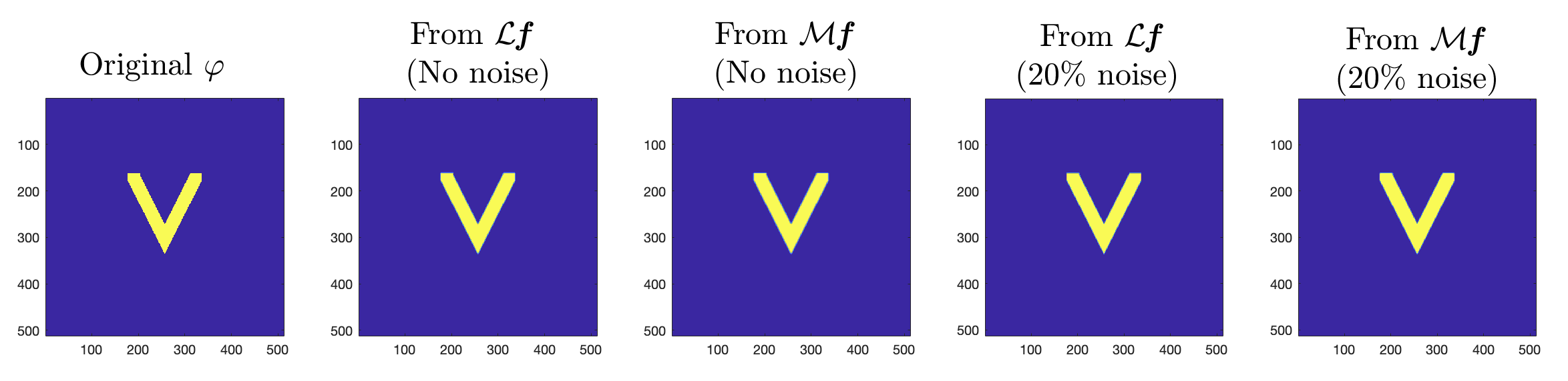
Figure 2: Recovery of $\varphi$ when f=$\mathrm{d}^{2}\varphi$ using formula (32)

From $\mathcal{L}\textbf{{f}}$(No noise)	From $\mathcal{M}\textbf{{f}}$(No noise)	From $\mathcal{L}\textbf{{f}}$($20\%$ noise)	From $\mathcal{M}\textbf{{f}}$($20\%$ noise)
5.60%	4.99%	10.91%	36.61%

Table 3: Relative errors of reconstruction of $\varphi$ from $\mathcal{L}\textbf{{f}}$ or $\mathcal{M}\textbf{{f}}$ when $\textbf{{f}}=\mathrm{d}^{2}\varphi$

The reconstruction for formulas (34) and (35) are shown in Figures 3, 4 and 5. Depending on the choice of u, the PDE appearing in (35) is elliptic $\displaystyle\left(\textbf{{u}}=(\cos{\pi/6},\sin{\pi/6})\right)$, parabolic $\displaystyle\left(\textbf{{u}}=(\cos{\pi/4},\sin{\pi/4})\right)$, and hyperbolic $\displaystyle\left(\textbf{{u}}=(\cos{\pi/3},\sin{\pi/3})\right)$. The numerical solution of such PDEs is discussed in Section 3. As shown, the reconstructions, even with $10\%$, are very quite good, and therefore, we chose not to put the reconstructions without noise. The relative errors are given for the no-noise case also in the tables.

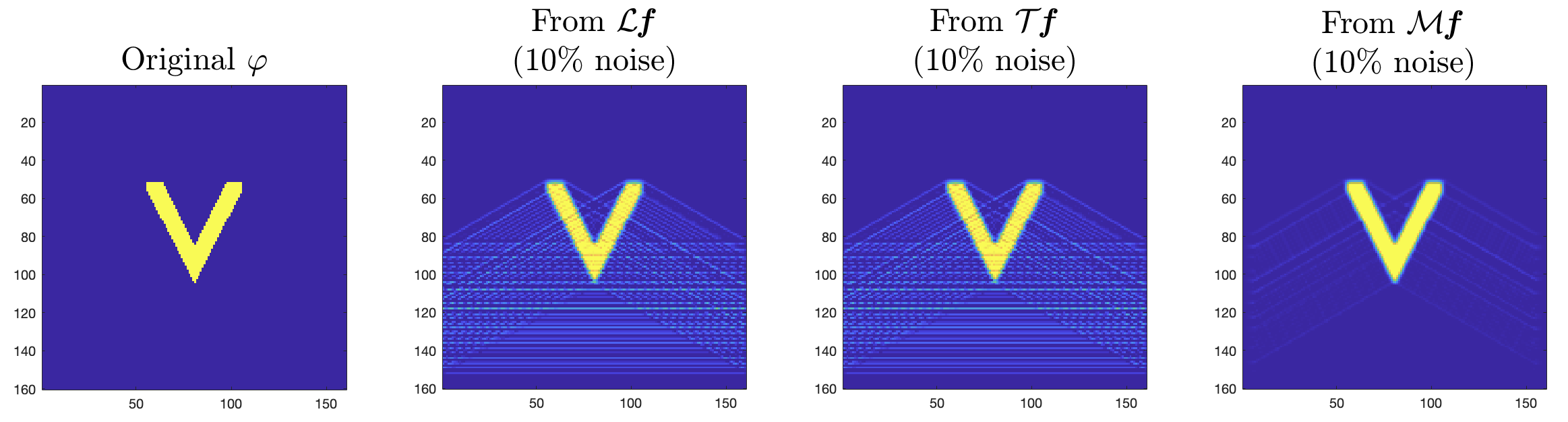
Figure 3: Recovery of $\varphi$ when f=$\mathrm{d}\mathrm{d}^{\perp}\varphi$ and $u_{1}>u_{2}$(Elliptic) with $10\%$ noise using formulas (34),(35)

	From $\mathcal{L}\textbf{{f}}$	From $\mathcal{T}\textbf{{f}}$	From $\mathcal{M}\textbf{{f}}$
No Noise	79.09%	79.09%	12.37%
$10\%$ Noise	81.40%	80.66%	17.45%

Table 4: Relative errors of reconstruction of $\varphi$ from $\mathcal{L}\textbf{{f}}$, $\mathcal{T}\textbf{{f}}$ or $\mathcal{M}\textbf{{f}}$ when $\textbf{{f}}=\mathrm{d}\mathrm{d}^{\perp}\varphi$ and $u_{1}>u_{2}$

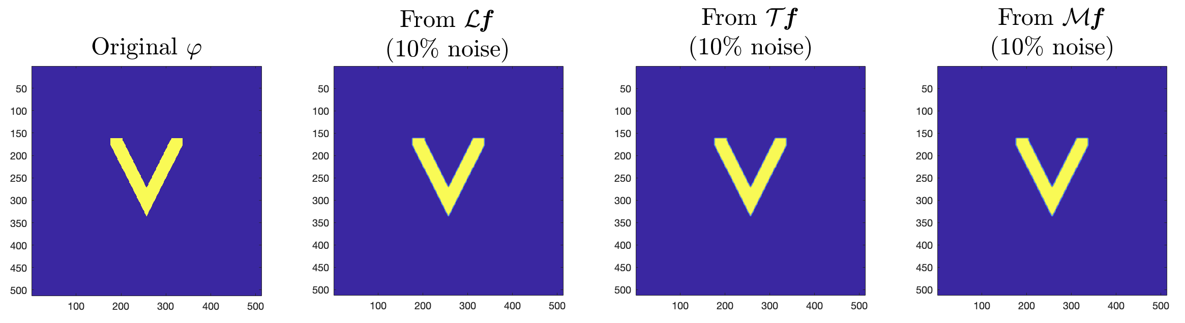
Figure 4: Recovery of $\varphi$ when f=$\mathrm{d}\mathrm{d}^{\perp}\varphi$ and $u_{1}=u_{2}$ (Parabolic) with $10\%$ noise using formulas (34),(35)

	From $\mathcal{L}\textbf{{f}}$	From $\mathcal{T}\textbf{{f}}$	From $\mathcal{M}\textbf{{f}}$
No Noise	4.99%	4.99%	6.03%
$10\%$ Noise	7.48%	5.13%	7.65%

Table 5: Relative errors of reconstruction of $\varphi$ from $\mathcal{L}\textbf{{f}}$, $\mathcal{T}\textbf{{f}}$ or $\mathcal{M}\textbf{{f}}$ when $\textbf{{f}}=\mathrm{d}\mathrm{d}^{\perp}\varphi$ and $u_{1}=u_{2}$

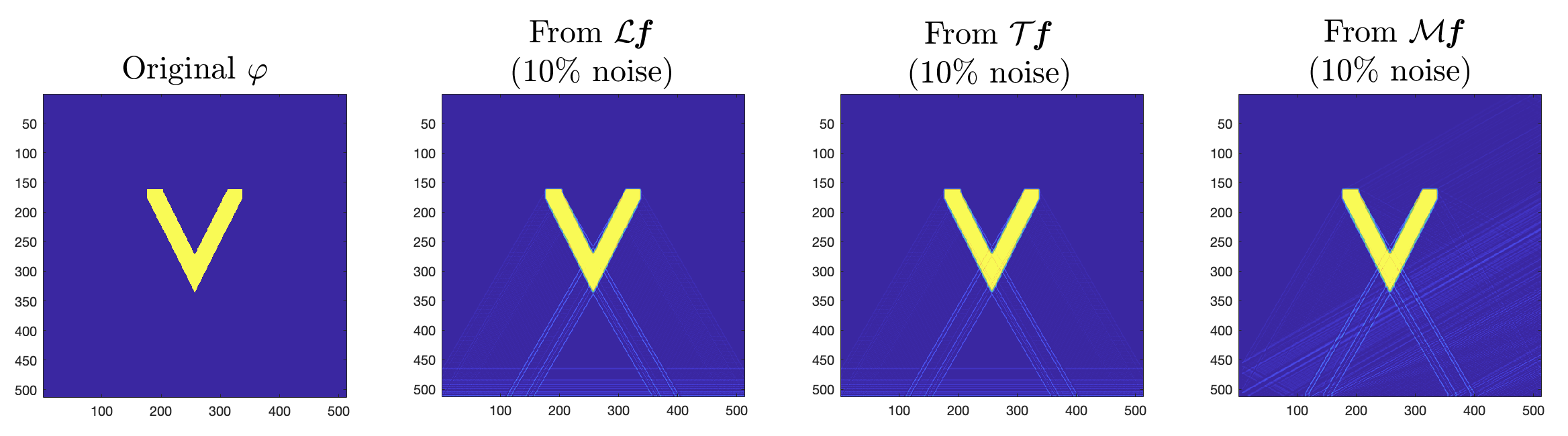
Figure 5: Recovery of $\varphi$ when f=$\mathrm{d}\mathrm{d}^{\perp}\varphi$ and $u_{1}<u_{2}$ (Hyperbolic) with $10\%$ noise using formulas (34),(35)

	From $\mathcal{L}\textbf{{f}}$	From $\mathcal{T}\textbf{{f}}$	From $\mathcal{M}\textbf{{f}}$
No Noise	12.09%	12.09%	7.89%
$10\%$ Noise	30.39%	14.02%	14.66%

Table 6: Relative errors of reconstruction of $\varphi$ from $\mathcal{L}\textbf{{f}}$, $\mathcal{T}\textbf{{f}}$ or $\mathcal{M}\textbf{{f}}$ when $\textbf{{f}}=\mathrm{d}\mathrm{d}^{\perp}\varphi$ and $u_{1}<u_{2}$

4.1.2 Tensor fields of the form $\textbf{{f}}=\mathrm{d}\textbf{{g}}$ or $\textbf{{f}}=\mathrm{d}^{\perp}\textbf{{g}}$

In this subsection, we consider 2-tensor field $\textbf{{f}}=\mathrm{d}\textbf{{g}}~{}\text{or}~{}\mathrm{d}^{\perp}\textbf{{g}}$ where g is a vector field and show the reconstructions of g from the combinations of V-line transforms obtained in [8] with and without noise. Since the reconstructions in the case $\textbf{{f}}=\mathrm{d}^{\perp}\textbf{{g}}$ are almost the same as in the case $\textbf{{f}}=\mathrm{d}\textbf{{g}}$, we have not included the reconstruction pictures for $\mathrm{d}^{\perp}\textbf{{g}}.$

Theorem 2.

Let $\textbf{{g}}=(g_{1},g_{2})$ be a vector field with components $g_{i}(\textbf{{x}})\in C_{c}^{2}(D_{1})$, for $i=1,2$.

• If f is a symmetric 2-tensor field of the form $\textbf{{f}}=\mathrm{d}\textbf{{g}}$, then it can be recovered explicitly in terms of $\mathcal{L}\textbf{{f}}$ and $\mathcal{M}\textbf{{f}}$ as

  $$g_{2}(\textbf{{x}})=-\frac{1}{2u_{2}}\mathcal{L}\textbf{{f}}(\textbf{{x}})$$ (36)

  $g_{1}$ recovered by solving a second-order partial differential equation

  $$2u_{1}^{2}\frac{\partial^{2}g_{1}}{\partial x_{1}^{2}}(\textbf{{x}})+(u_{1}^{2}-u_{2}^{2})\frac{\partial^{2}g_{1}}{\partial x_{2}^{2}}(\textbf{{x}})=-\frac{1}{2u_{2}}D_{\textbf{{u}}}D_{\textbf{{v}}}h(\textbf{{x}})$$

  where $\displaystyle h(\textbf{{x}})=2\mathcal{M}\textbf{{f}}(\textbf{{x}})+\mathcal{V}\left(\frac{\partial g_{2}}{\partial x_{1}}\right)(\textbf{{x}})$ with additional homogeneous boundary (or initial) conditions, which can be uniquely solved to get $g_{1}$. More explicitly, we have the following three cases:

  1. When $u_{1}^{2}>u_{2}^{2}$, we have an elliptic PDE

     $$2u_{1}^{2}\frac{\partial^{2}g_{1}}{\partial x_{1}^{2}}+\left(u_{1}^{2}-u_{2}^{2}\right)\frac{\partial^{2}g_{1}}{\partial x_{2}^{2}}=-\frac{1}{2u_{2}}D_{\textbf{{u}}}D_{\textbf{{v}}}h(\textbf{{x}})$$ (37)

     with homogeneous boundary conditions, which has a unique solution.

  2. When $u_{1}^{2}=u_{2}^{2}$, the above partial differential equation becomes:

     $$2u_{1}^{2}\frac{\partial^{2}g_{1}}{\partial x_{1}^{2}}(\textbf{{x}})=-\frac{1}{2u_{2}}D_{\textbf{{u}}}D_{\textbf{{v}}}h(\textbf{{x}}),$$ (38)

     which gives $g_{1}$ by integrating twice along $\textbf{{e}}_{1}$-direction.

  3. When $u_{1}^{2}<u_{2}^{2}$, we have a hyperbolic PDE

     $$2u_{1}^{2}\frac{\partial^{2}g_{1}}{\partial x_{1}^{2}}-\left(u_{2}^{2}-u_{1}^{2}\right)\frac{\partial^{2}g_{1}}{\partial x_{2}^{2}} =-\frac{1}{2u_{2}}D_{\textbf{{u}}}D_{\textbf{{v}}}h(\textbf{{x}}),$$ (39)

     which can be solved by choosing appropriate initial conditions on $g_{1}$ (for instance, we can take $g_{1}(a,y)=0$ and $\displaystyle\frac{\partial g_{1}}{\partial x_{1}}(a,y)=0$, for $y\in\mathbb{R}$ and any fixed $a\in\mathbb{R}\setminus[-1,1]$).

• If f is a symmetric 2-tensor field of the form $\textbf{{f}}=\mathrm{d}^{\perp}\textbf{{g}}$, then it can be recovered explicitly in terms of $\mathcal{T}\textbf{{f}}$ and $\mathcal{M}\textbf{{f}}$ as

  $$g_{1}(\textbf{{x}})=\frac{1}{2u_{2}}\mathcal{T}\textbf{{f}}(\textbf{{x}})$$ (40)

  $g_{2}$ is recovered by solving the following second-order partial differential equation (equipped with appropriate boundary or initial conditions):

  $$2u_{1}^{2}\frac{\partial^{2}g_{2}}{\partial x_{1}^{2}}(\textbf{{x}})+(u_{1}^{2}-u_{2}^{2})\frac{\partial^{2}g_{2}}{\partial x_{2}^{2}}(\textbf{{x}})=-\frac{1}{2u_{2}}D_{\textbf{{u}}}D_{\textbf{{v}}}\tilde{h}(\textbf{{x}}),$$ (41)

  where $\displaystyle\tilde{h}(\textbf{{x}})=-2\mathcal{M}\textbf{{f}}(\textbf{{x}})-\mathcal{V}\left(\frac{\partial g_{1}}{\partial x_{1}}\right)(\textbf{{x}})$.

In Figures 6,7 and 8, $g_{2}$ is reconstructed directly from $\mathcal{L}\textbf{{f}}$ (see (36)) and the recovery of $g_{1}$ requires solving an elliptic (for $\displaystyle\textbf{{u}}=(\cos{\pi/6},\sin{\pi/6})$, see (37)), parabolic (for $\displaystyle\textbf{{u}}=(\cos{\pi/4},\sin{\pi/4})$, see (38)), and hyperbolic (for $\displaystyle\textbf{{u}}=(\cos{\pi/3},\sin{\pi/3})$, see (39)) PDE, which we have already discussed in previous section. Figure 9 presents the reconstructions with different levels of noise for different cases (elliptic, parabolic, and hyperbolic). The same algorithms are used in Figures 10,11,12, and 13 for the non-smooth phantom.

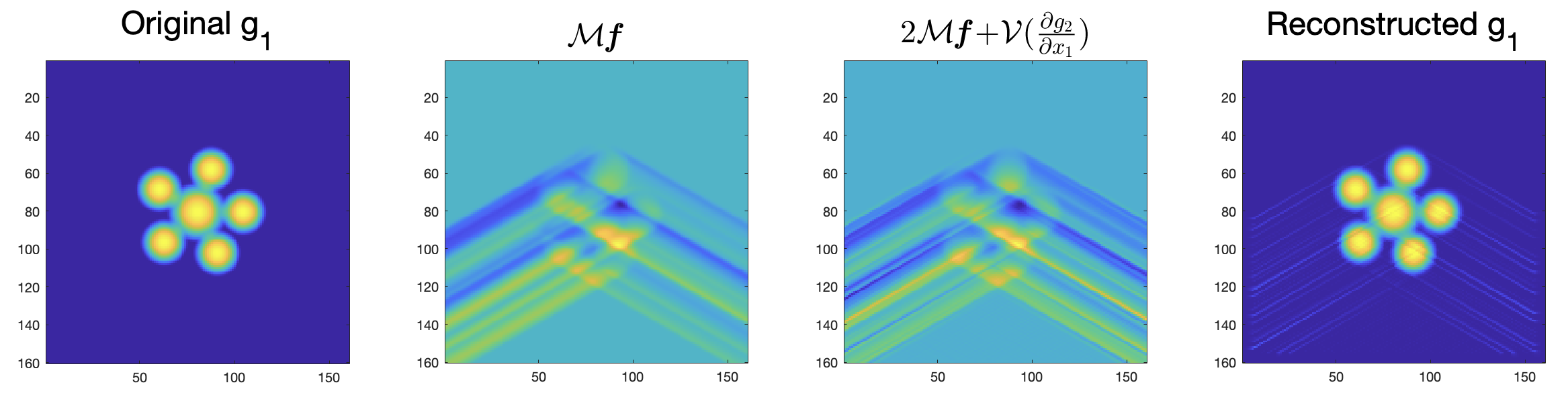
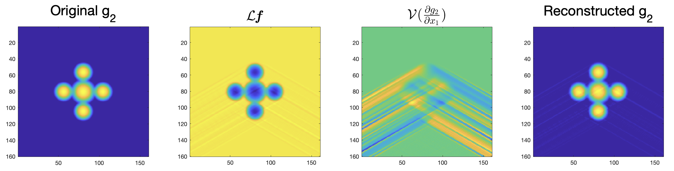
Figure 6: Recovery of g from $\mathcal{L}\textbf{{f}}$ and $\mathcal{M}\textbf{{f}}$ when $\textbf{{f}}=\mathrm{d}\textbf{{g}}$ and $u_{1}>u_{2}$ (Elliptic) using formulas (36)(37).

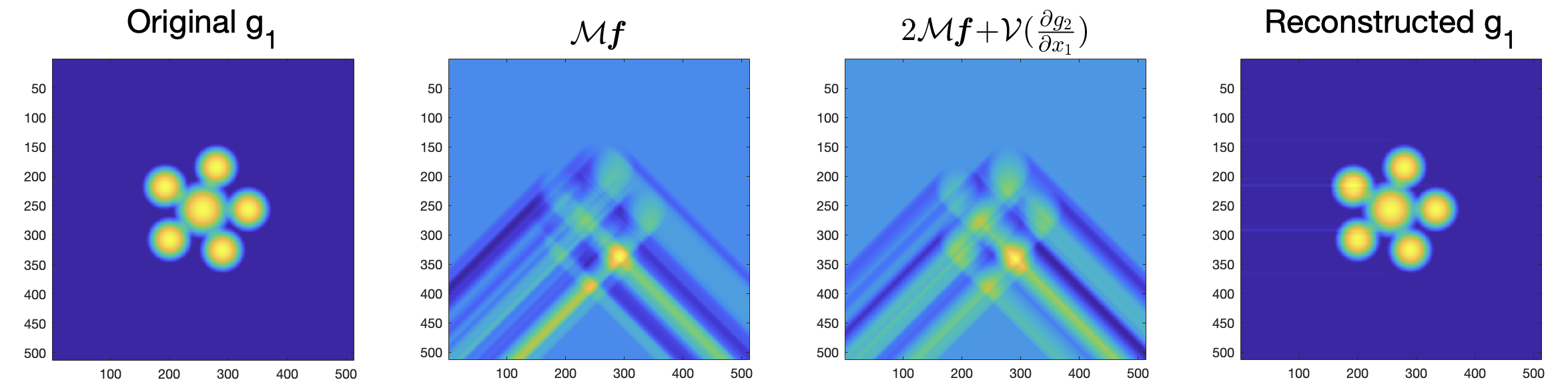
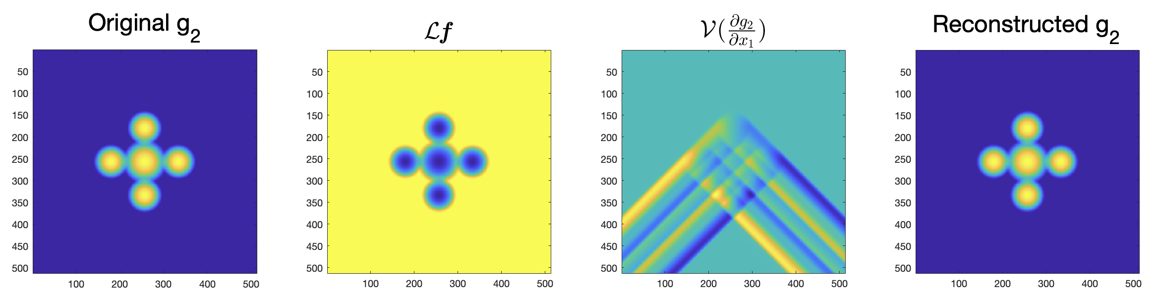
Figure 7: Recovery of g from $\mathcal{L}\textbf{{f}}$ and $\mathcal{M}\textbf{{f}}$ when $\textbf{{f}}=\mathrm{d}\textbf{{g}}$ and $u_{1}=u_{2}$ (Parabolic) using formulas (36)(38)

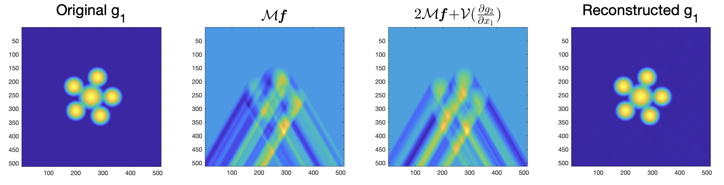
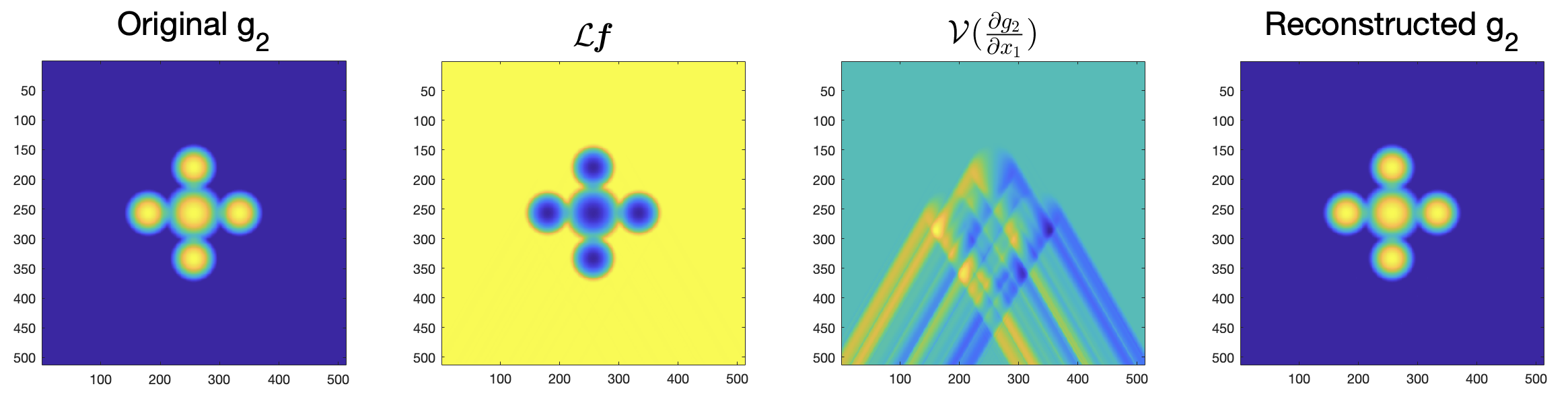
Figure 8: Recovery of g from $\mathcal{L}\textbf{{f}}$ and $\mathcal{M}\textbf{{f}}$ when $\textbf{{f}}=\mathrm{d}\textbf{{g}}$ and $u_{1}<u_{2}$ (Hyperbolic) using formulas (36)(39).

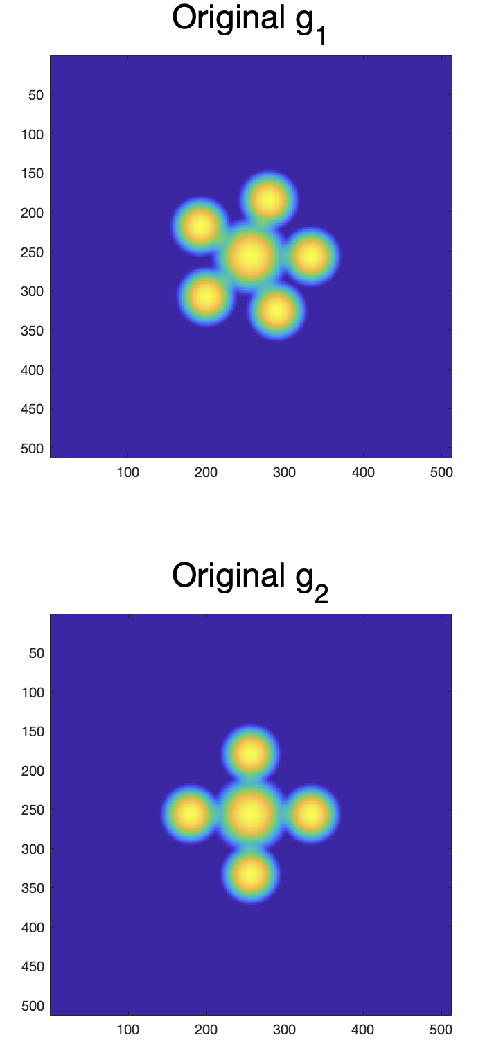
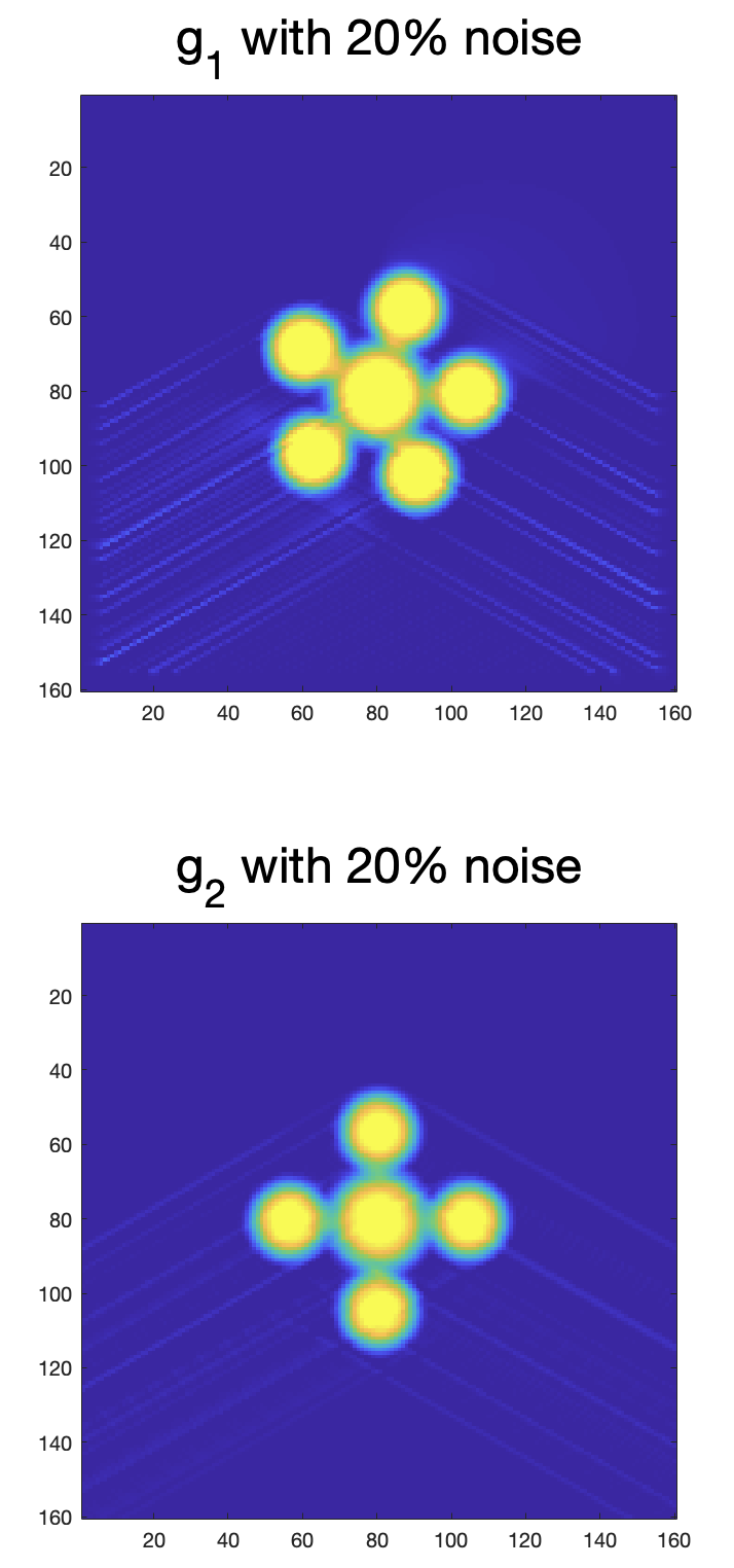
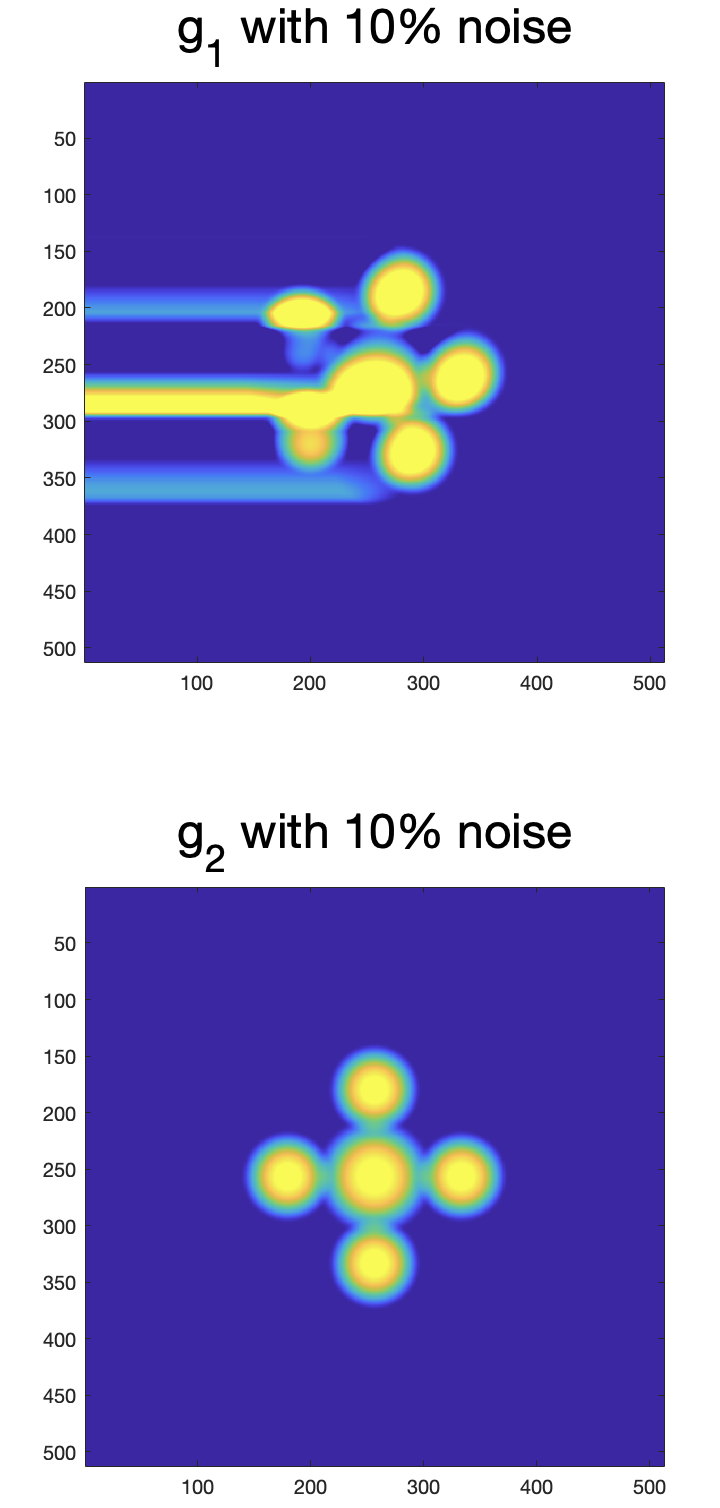
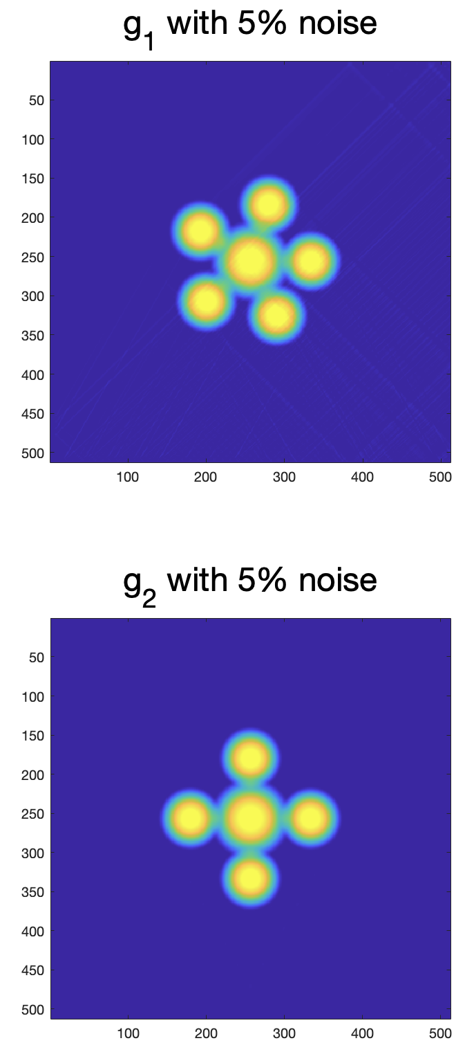
Figure 9: (Column 1) Original $g_{1},g_{2}$, (Column 2) Reconstructed $g_{1},g_{2}$ when $u_{1}>u_{2}$ with $20\%$ noise, (Column 3) Reconstructed $g_{1},g_{2}$ when $u_{1}=u_{2}$ with $10\%$ noise, (Column 4) Reconstructed $g_{1},g_{2}$ when $u_{1}<u_{2}$ with $5\%$ noise.

g	$20\%$ Noise - Elliptic	$10\%$ Noise - Parabolic	$5\%$ Noise - Hyperbolic
$g_{1}$	33.75%	128.56%	7.60%
$g_{2}$	13.80%	7.17%	6.99%

Table 7: Relative errors of reconstruction of g from $\mathcal{L}\textbf{{f}}$ and $\mathcal{M}\textbf{{f}}$ when $\textbf{{f}}=\mathrm{d}\textbf{{g}}$

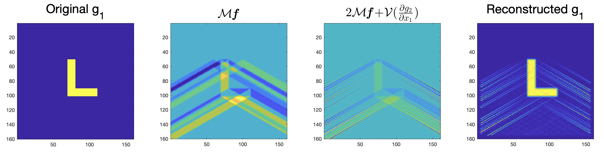
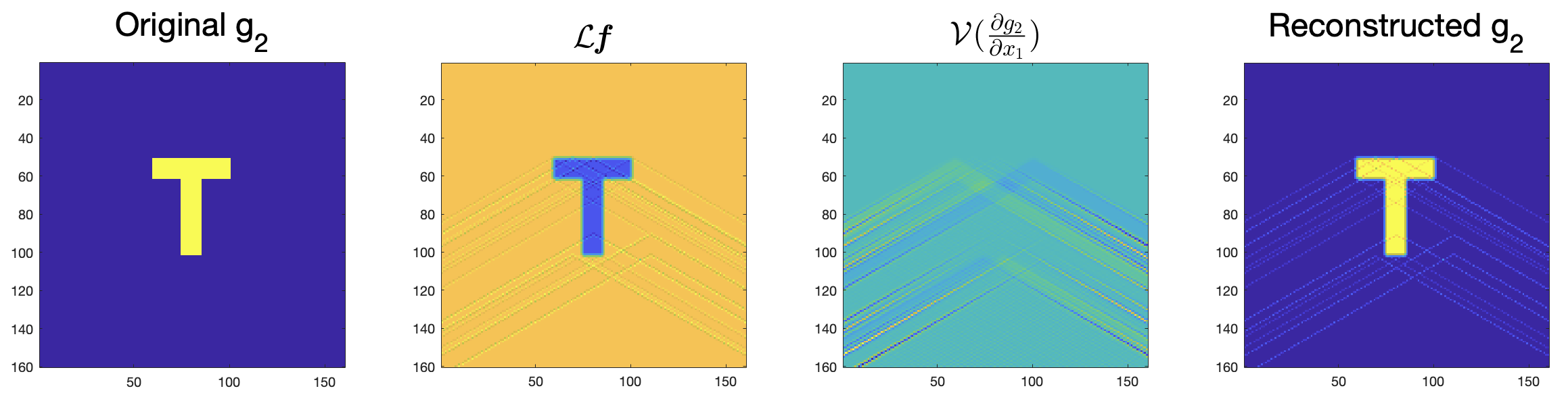
Figure 10: Recovery of g from $\mathcal{L}\textbf{{f}}$ and $\mathcal{M}\textbf{{f}}$ when $\textbf{{f}}=\mathrm{d}\textbf{{g}}$ and $u_{1}>u_{2}$ (Elliptic) using formulas (36)(37).

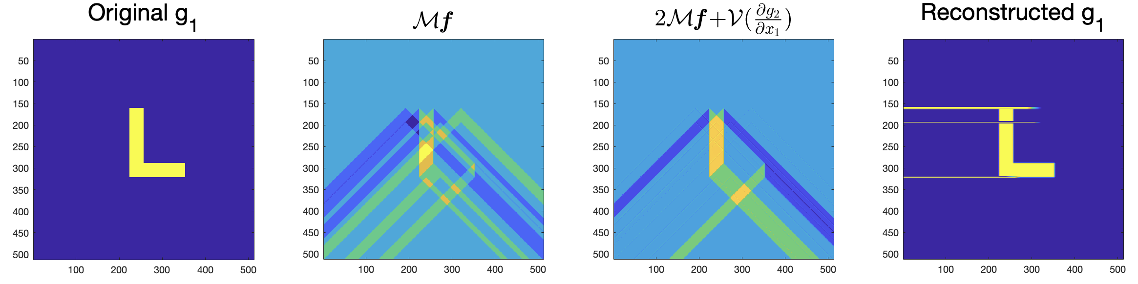
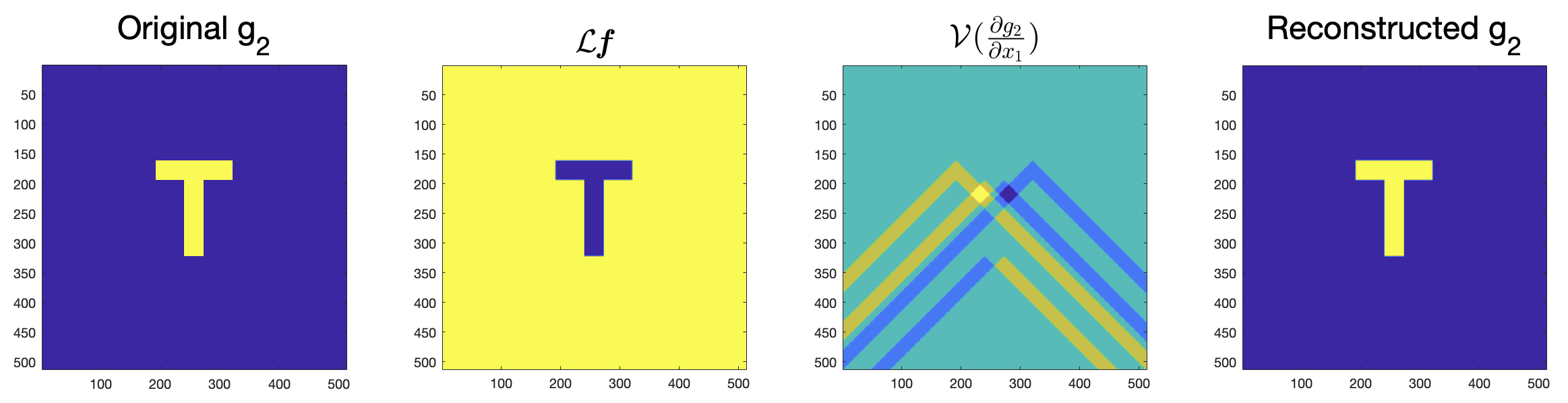
Figure 11: Recovery of g from $\mathcal{L}\textbf{{f}}$ and $\mathcal{M}\textbf{{f}}$ when $\textbf{{f}}=\mathrm{d}\textbf{{g}}$ and $u_{1}=u_{2}$ (Parabolic) using formulas (36)(38).

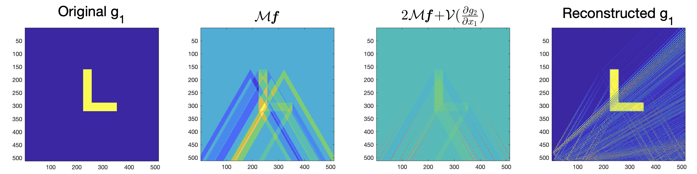
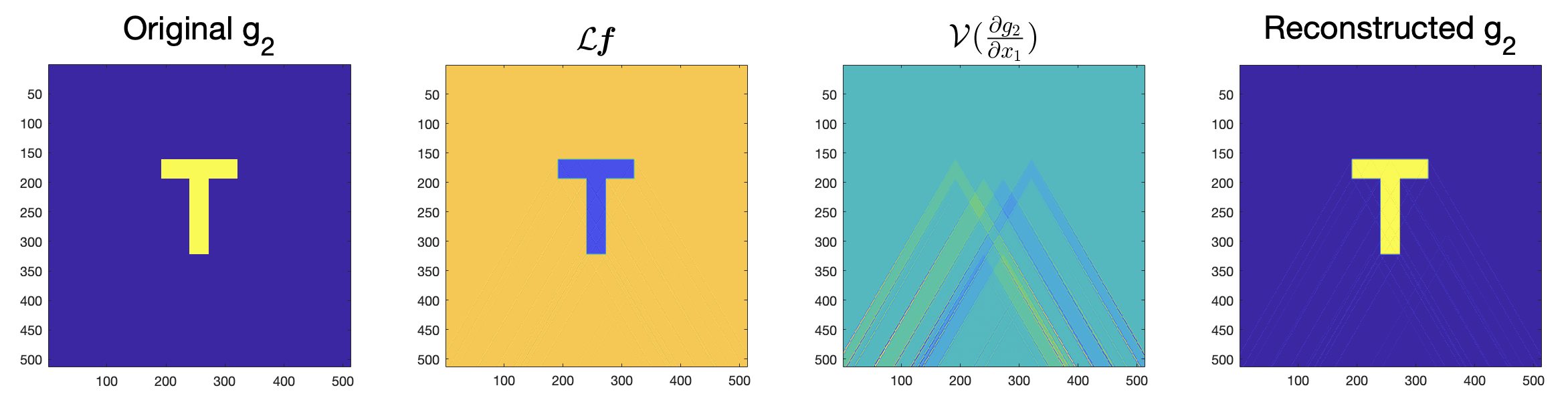
Figure 12: Recovery of g from $\mathcal{L}\textbf{{f}}$ and $\mathcal{M}\textbf{{f}}$ when $\textbf{{f}}=\mathrm{d}\textbf{{g}}$ and $u_{1}<u_{2}$ (Hyperbolic) using formulas (36)(39).

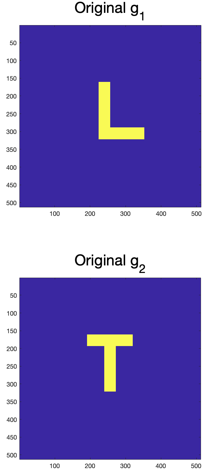
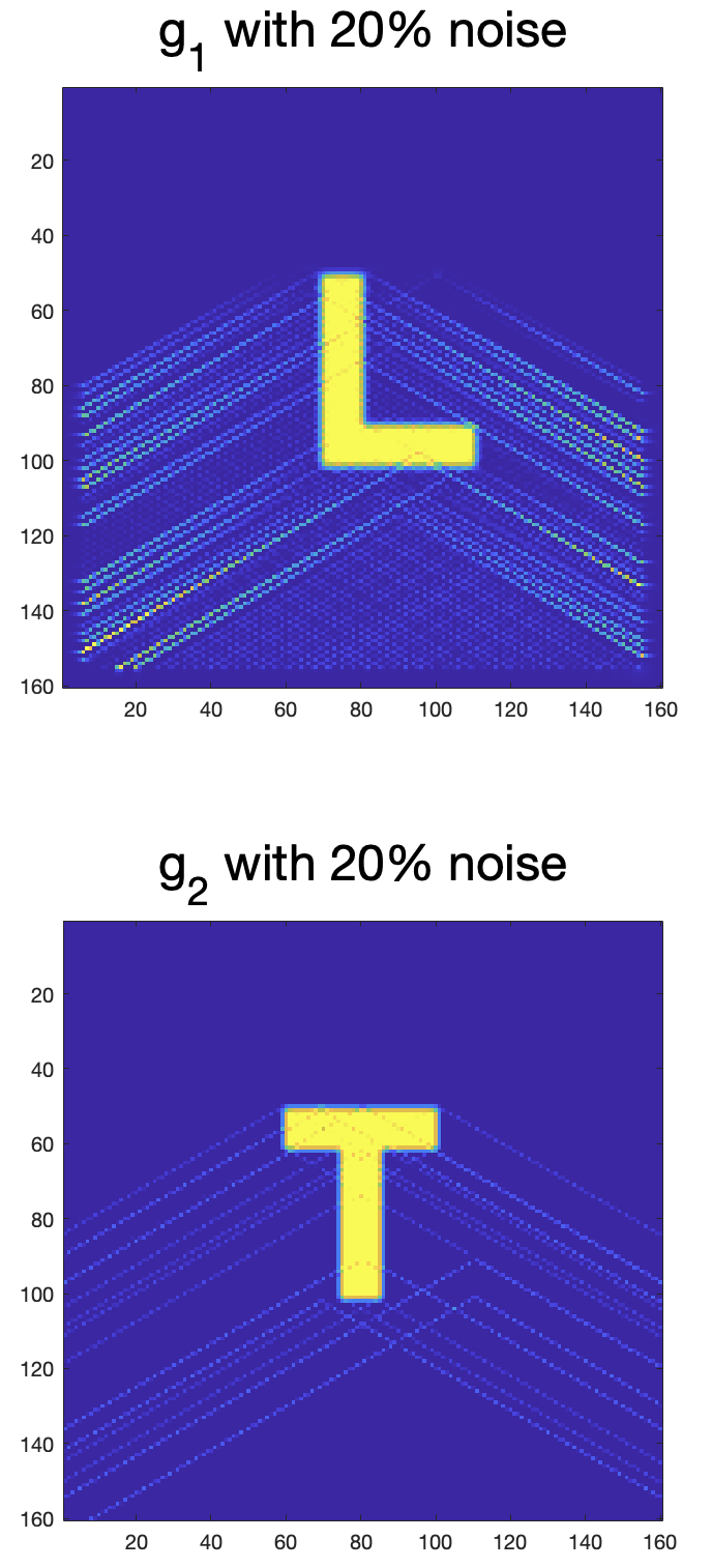
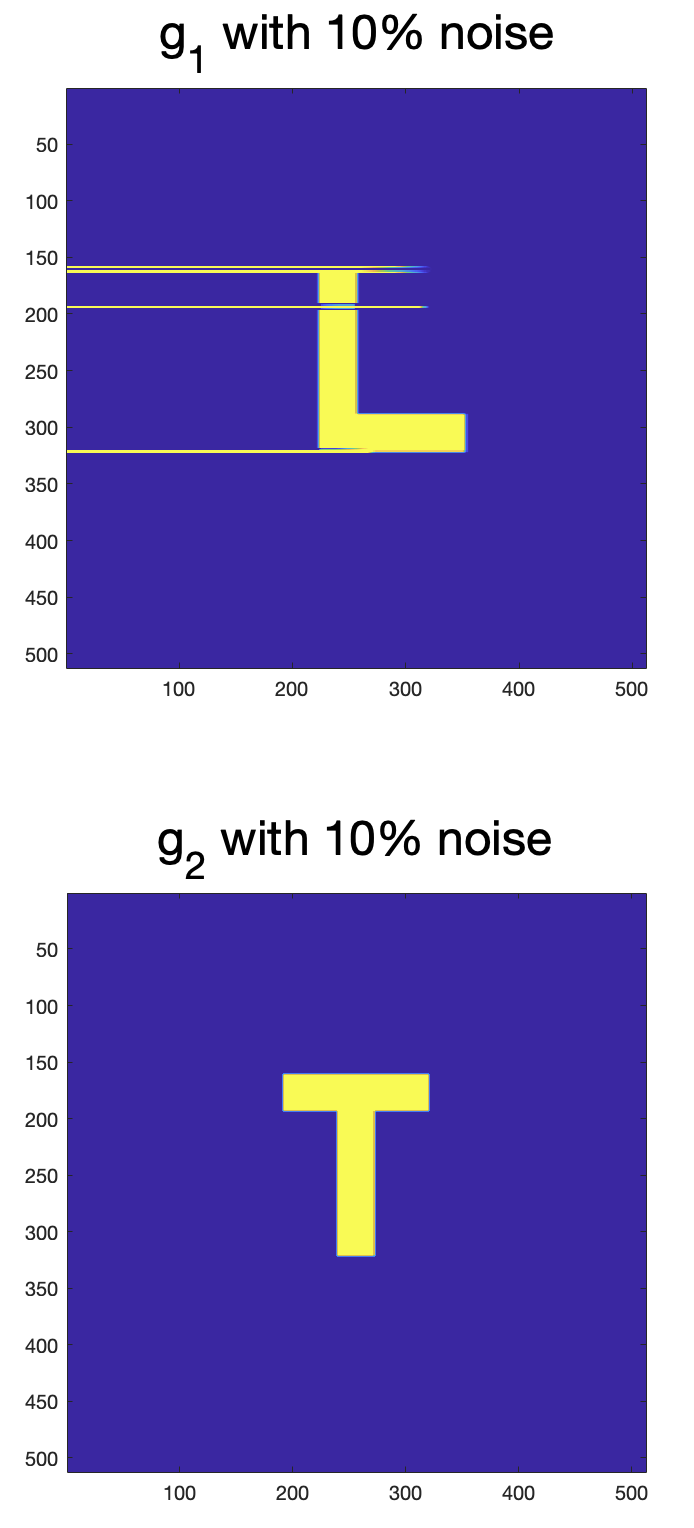
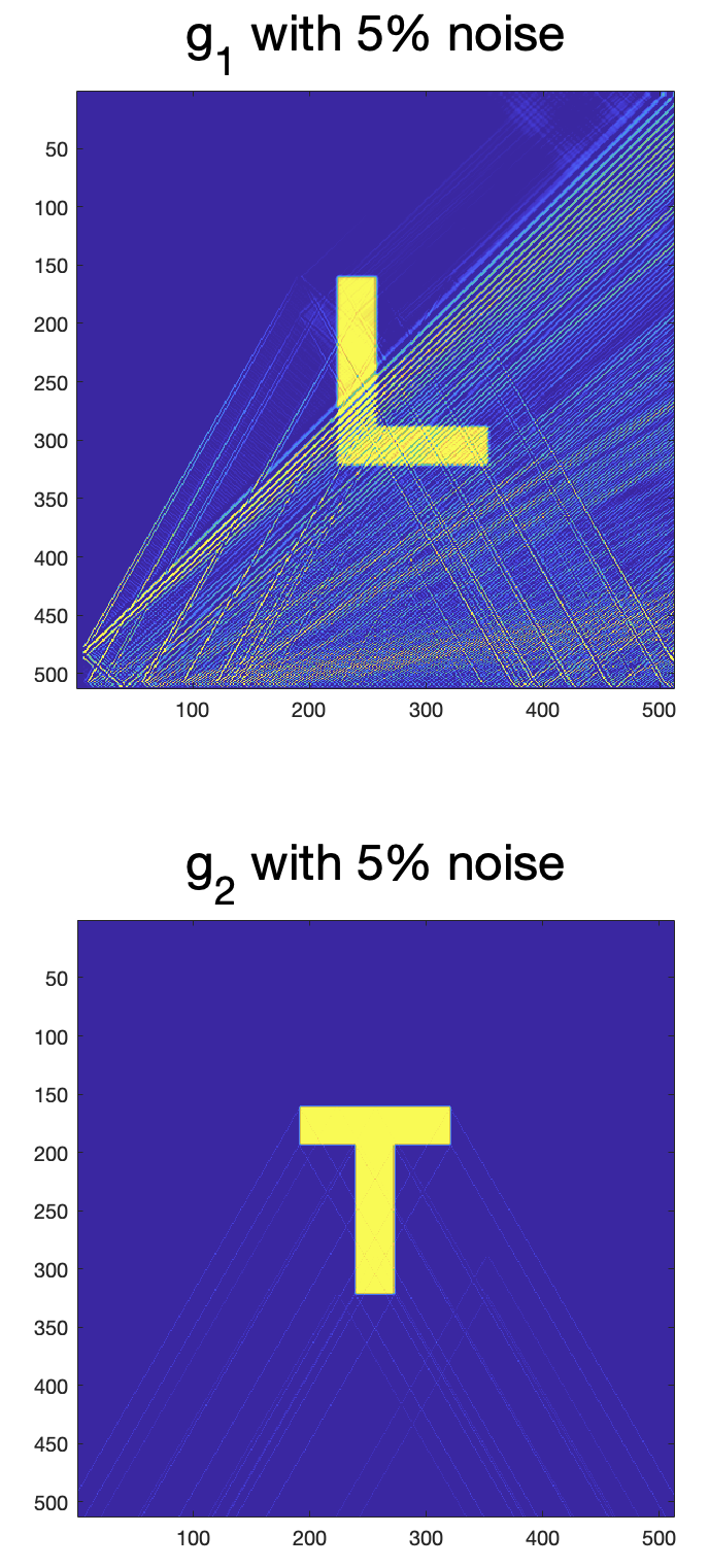
Figure 13: (Column 1) Original $g_{1},g_{2}$, (Column 2) Recons. $g_{1},g_{2}$ ($u_{1}>u_{2}$) with $20\%$ noise, (Column 3) Recons. $g_{1},g_{2}$ ($u_{1}=u_{2}$) with $10\%$ noise, (Column 4) Recons. $g_{1},g_{2}$ ($u_{1}<u_{2}$) with $5\%$ noise.

g	$20\%$ Noise - Elliptic	$10\%$ Noise - Parabolic	$5\%$ Noise -Hyperbolic
$g_{1}$	30.54%	533.80%	46.15%
$g_{2}$	13.55%	8.73%	7.88%

Table 8: Relative errors of reconstruction of g from $\mathcal{L}\textbf{{f}}$ and $\mathcal{M}\textbf{{f}}$ when $\textbf{{f}}=\mathrm{d}\textbf{{g}}$

4.2 Full Recovery of f from $\mathcal{L}\textbf{{f}},\mathcal{T}\textbf{{f}}$ and $\mathcal{M}\textbf{{f}}$

In this subsection, we consider $\mathcal{L}\textbf{{f}},\mathcal{T}\textbf{{f}}$ and $\mathcal{M}\textbf{{f}}$ to recover $\textbf{{f}}.$ As in the previous sections, we start by discussing the theoretical results for this in Theorem 3.

Theorem 3.

Consider a symmetric $2$-tensor field $\textbf{{f}}\in C_{c}^{2}\left(S^{2};D_{1}\right)$. Then,

• For $u_{1}=u_{2},$ f can be recovered from $\mathcal{L}\textbf{{f}},\mathcal{T}\textbf{{f}}$ and $\mathcal{M}\textbf{{f}}$ by

  $$f_{11}(\textbf{{x}}) =\frac{1}{4u_{2}}D_{\textbf{{u}}}D_{\textbf{{v}}}\mathcal{X}_{\textbf{{e}}_{2}}\left(\mathcal{L}\textbf{{f}}+\mathcal{T}\textbf{{f}}\right)(\textbf{{x}})-\frac{1}{2u_{1}}D_{\textbf{{u}}}D_{\textbf{{v}}}\mathcal{X}_{-\textbf{{e}}_{1}}\mathcal{M}\textbf{{f}}\,(\textbf{{x}}),$$ (42)

  $$f_{12}(\textbf{{x}}) =\frac{1}{4u_{1}}D_{\textbf{{u}}}D_{\textbf{{v}}}\mathcal{X}_{-\textbf{{e}}_{1}}\left(\mathcal{L}\textbf{{f}}-\mathcal{T}\textbf{{f}}\right)(\textbf{{x}}),$$ (43)

  $$f_{22}(\textbf{{x}}) =\frac{1}{4u_{2}}D_{\textbf{{u}}}D_{\textbf{{v}}}\mathcal{X}_{\textbf{{e}}_{2}}\left(\mathcal{L}\textbf{{f}}+\mathcal{T}\textbf{{f}}\right)(\textbf{{x}})+\frac{1}{2u_{1}}D_{\textbf{{u}}}D_{\textbf{{v}}}\mathcal{X}_{-\textbf{{e}}_{1}}\mathcal{M}\textbf{{f}}\,(\textbf{{x}}).$$ (44)

  where $\textbf{{e}}_{1}=(1,0)$ and $\textbf{{e}}_{2}=(0,1)$.

• For $u_{1}\neq u_{2},$ f can be reconstructed from $\mathcal{L}\textbf{{f}},\mathcal{T}\textbf{{f}}$ and $\mathcal{M}\textbf{{f}}$ as following: $f_{12}$ can be found by solving the following elliptic boundary value problem:

  $$\left\{\begin{array}[]{rll}a\partial_{x_{1}}^{2}f_{12}+b\partial_{x_{2}}^{2}f_{12}&=-g&\mbox{ in }D_{1},\\ f_{12}&=0&\mbox{ on }\partial D_{1}.\end{array}\right.$$ (47)

  where $a=2u_{1}^{2}\left[1+(u_{1}^{2}-u_{2}^{2})\right]>0$,   $b=\left(u_{1}^{2}-u_{2}^{2}\right)^{2}>0$ (since $u_{1}\neq u_{2}$), and

  $$g=\frac{1}{2u_{2}}\left[u_{1}^{2}\partial_{x_{1}}D_{\textbf{{u}}}D_{\textbf{{v}}}\left(\mathcal{T}\textbf{{f}}-\mathcal{L}\textbf{{f}}\right)+(u_{1}^{2}-u_{2}^{2})\partial_{x_{2}}D_{\textbf{{u}}}D_{\textbf{{v}}}\mathcal{M}\textbf{{f}}\right]$$

  $f_{11}$ can be recover from the knowledge of $\mathcal{L}\textbf{{f}},\mathcal{T}\textbf{{f}}$ and reconstructed $f_{12}$ by

  $$f_{11}=-\mathcal{X}_{\textbf{{e}}_{2}}\left[\left(u_{2}^{2}D_{\textbf{{u}}}D_{\textbf{{v}}}\mathcal{T}\textbf{{f}}-u_{1}^{2}D_{\textbf{{u}}}D_{\textbf{{v}}}\mathcal{L}\textbf{{f}}+4u_{1}^{2}u_{2}\partial_{x_{1}}f_{12}\right)/\left(2u_{2}(u_{1}^{2}-u_{2}^{2})\right)\right].$$ (48)

  $f_{22}$ can be recovered from $\mathcal{L}\textbf{{f}},\mathcal{T}\textbf{{f}}$ and reconstructed $f_{11}$ by

  $$f_{22}(\textbf{{x}})=\frac{1}{2u_{2}}D_{\textbf{{u}}}D_{\textbf{{v}}}\mathcal{X}_{\textbf{{e}}_{2}}\left(\mathcal{L}\textbf{{f}}+\mathcal{T}\textbf{{f}}\right)(\textbf{{x}})-f_{11}(\textbf{{x}})$$ (49)

  where $\textbf{{e}}_{2}=(0,1)$.

The Figures 14 demonstrates the reconstruction obtained by applying formulas (42),(43) and (44) for the non-smooth phantom. Figure 15 shows the corresponding reconstructions in the presence of different levels of noise.

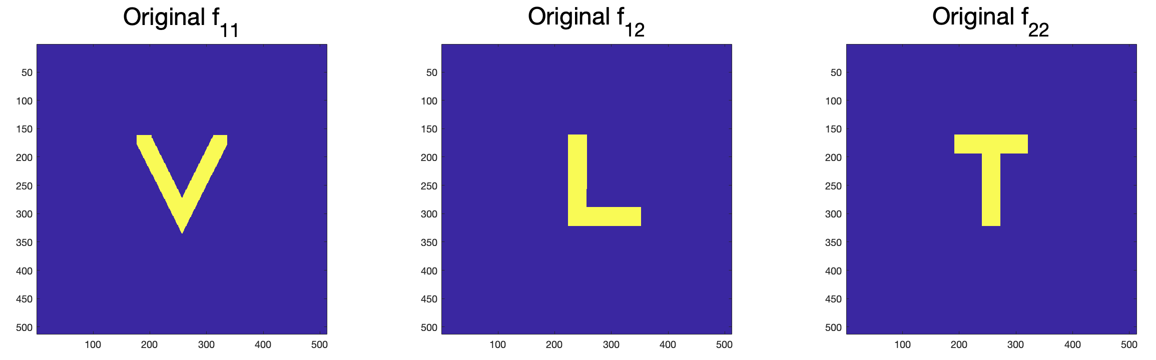
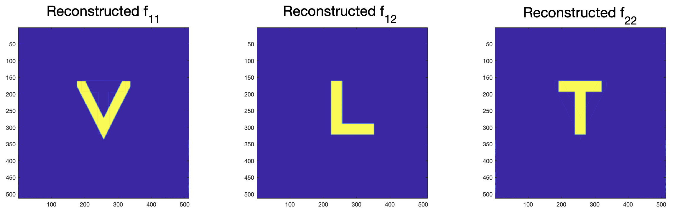
Figure 14: Components of f(Row 1), longitudinal ($\mathcal{L}\textbf{{f}}$), mixed($\mathcal{M}\textbf{{f}}$) and transverse ($\mathcal{T}\textbf{{f}}$) V-line transforms of f (Row 2), reconstructed components of f when $\textbf{{u}}=(\cos{\pi/4,\sin{\pi/4}})$ using formulas (42),(43),(44) (Row 3).

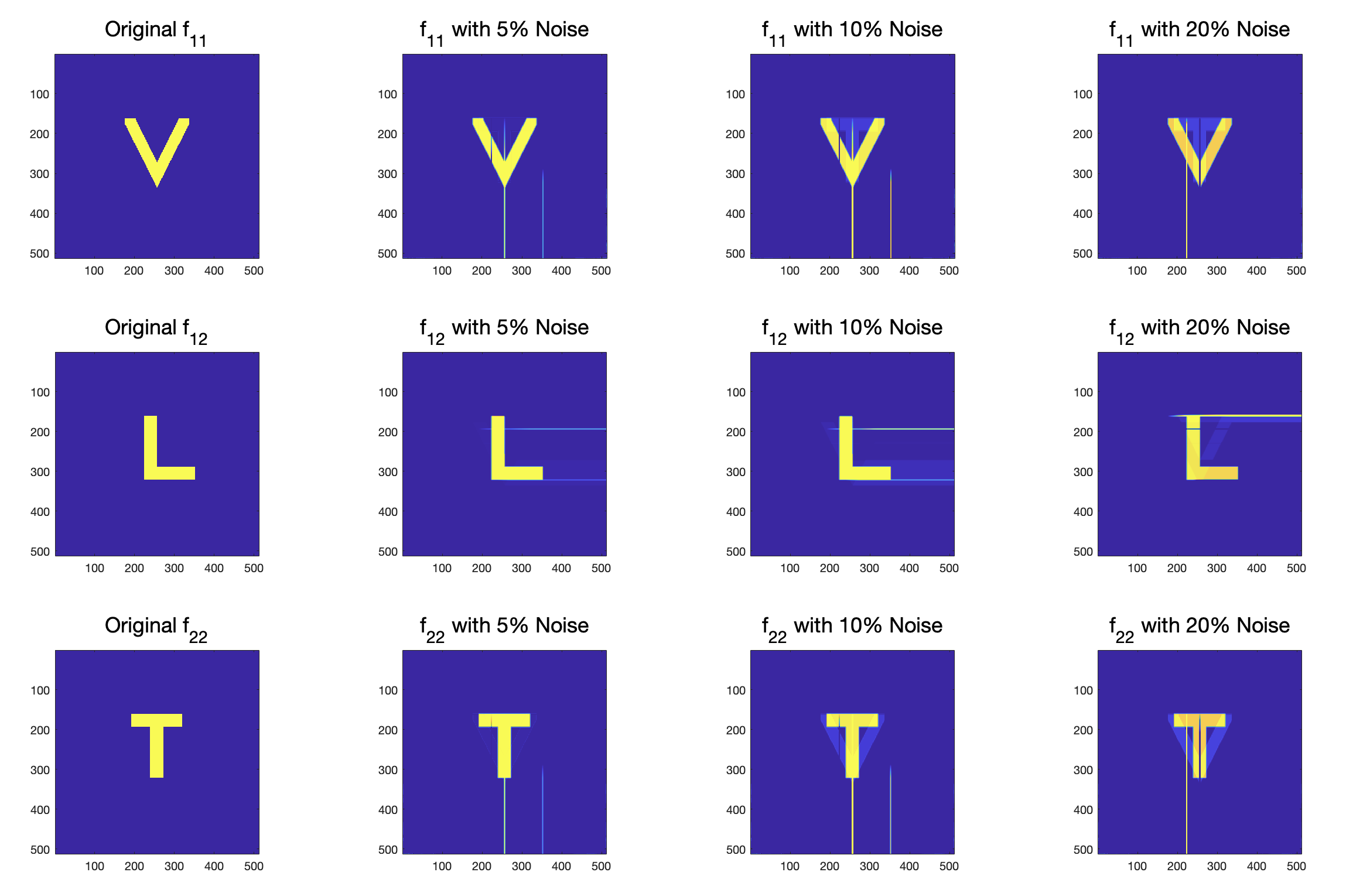
Figure 15: Reconstruction of f from $\mathcal{L}\textbf{{f}},\mathcal{M}\textbf{{f}},\mathcal{T}\textbf{{f}}$ when $\textbf{{u}}=(\cos{\pi/4},\sin{\pi/4})$ with $5\%,10\%$ and $20\%$ noise

f	No noise	$5\%$ Noise	$10\%$ Noise	$20\%$ Noise
$f_{11}$	5.22%	85.56%	194.44%	452.72%
$f_{12}$	9.42%	30.25%	68.14%	158.89%
$f_{22}$	8.15%	65.07%	146.95%	344.88%

Table 9: Relative errors of reconstruction of $f_{11},f_{12},f_{22}$ from $\mathcal{L}\textbf{{f}},\mathcal{M}\textbf{{f}}$ and $\mathcal{T}\textbf{{f}}$ when $\textbf{{u}}=(\cos{\pi/4,\sin{\pi/4}})$

We took $\textbf{{u}}=(\cos{\pi/3,\sin{\pi/3}})$ for implementations of (47), (48), and (49) which is shown in Figures 16 and 18 for the smooth phantom and non-smooth phantoms, respectively. Corresponding reconstructions in the presence of various levels of noise are presented in Figures 17 and 19.

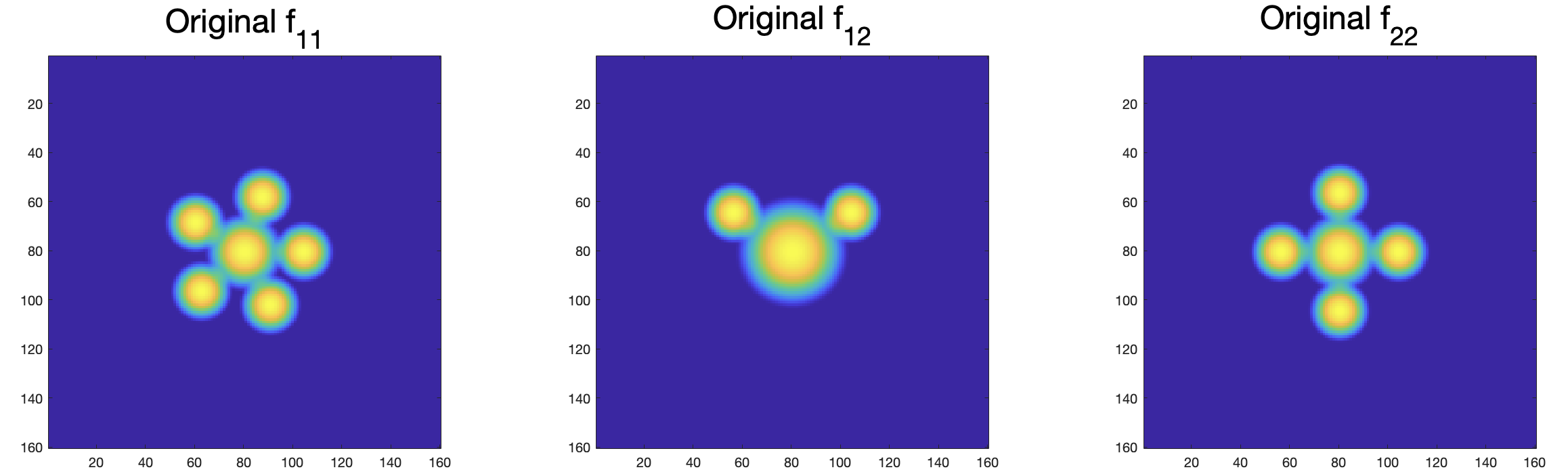
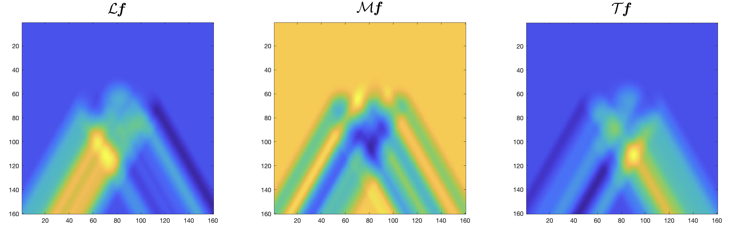
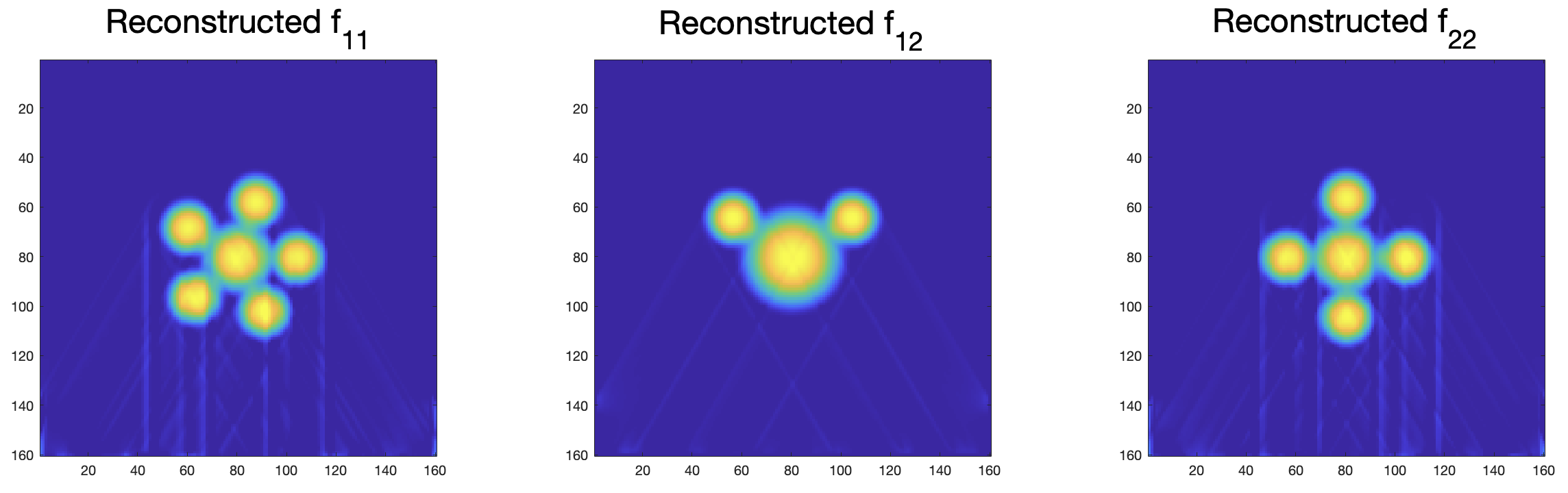
Figure 16: Components of f(Row 1), longitudinal ($\mathcal{L}\textbf{{f}}$), mixed($\mathcal{M}\textbf{{f}}$) and transverse ($\mathcal{T}\textbf{{f}}$) V-line transforms of f (Row 2), reconstructed components of f when $\textbf{{u}}=(\cos{\pi/3,\sin{\pi/3}})$ using formulas (47),(48),(49) (Row 3).

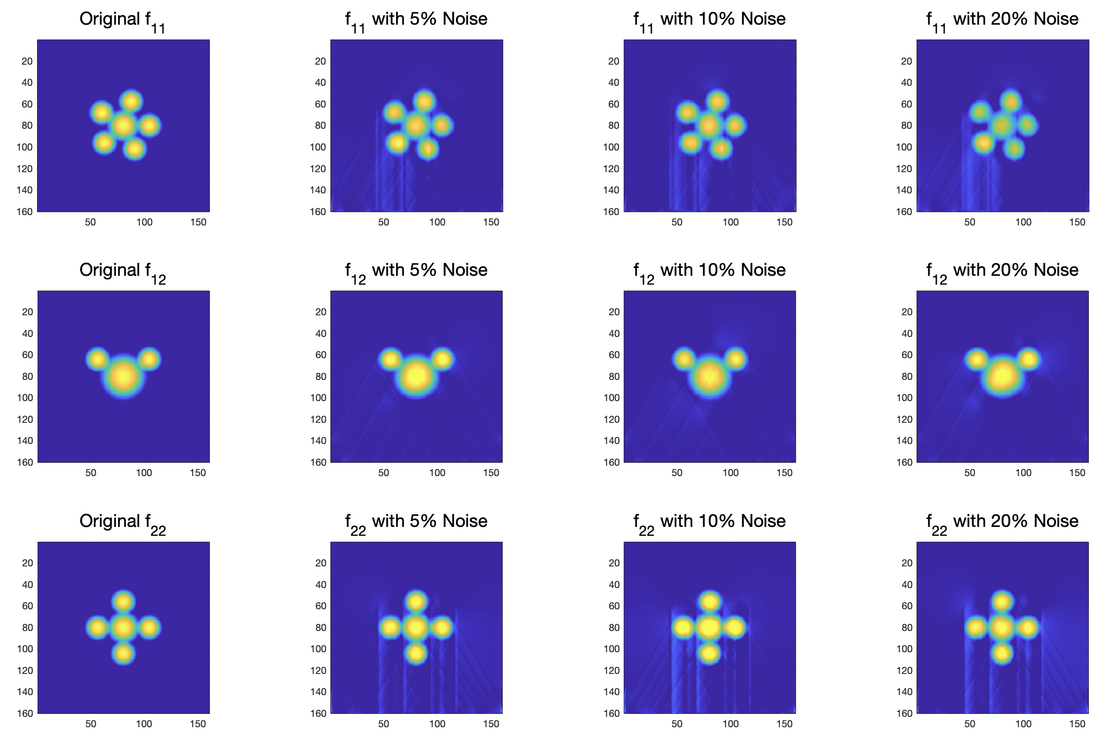
Figure 17: Reconstruction of f from $\mathcal{L}\textbf{{f}},\mathcal{M}\textbf{{f}},\mathcal{T}\textbf{{f}}$ when $\textbf{{u}}=(\cos{\pi/3},\sin{\pi/3})$ with $5\%,10\%$ and $20\%$ noise

f	No noise	$5\%$ Noise	$10\%$ Noise	$20\%$ Noise
$f_{11}$	8.49%	16.27%	18.60%	30.64%
$f_{12}$	1.84%	8.62%	6.45%	9.54%
$f_{22}$	8.77%	15.20%	25.15%	21.34%

Table 10: Relative errors of reconstruction of $f_{11},f_{12},f_{22}$ from $\mathcal{L}\textbf{{f}},\mathcal{M}\textbf{{f}}$ and $\mathcal{T}\textbf{{f}}$ when $\textbf{{u}}=(\cos{\pi/3,\sin{\pi/3}})$

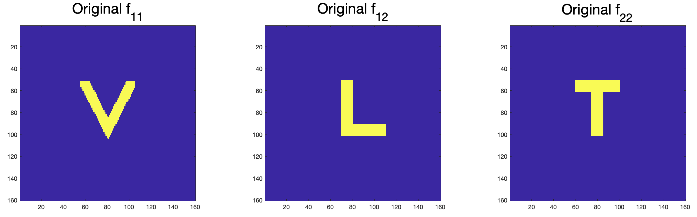
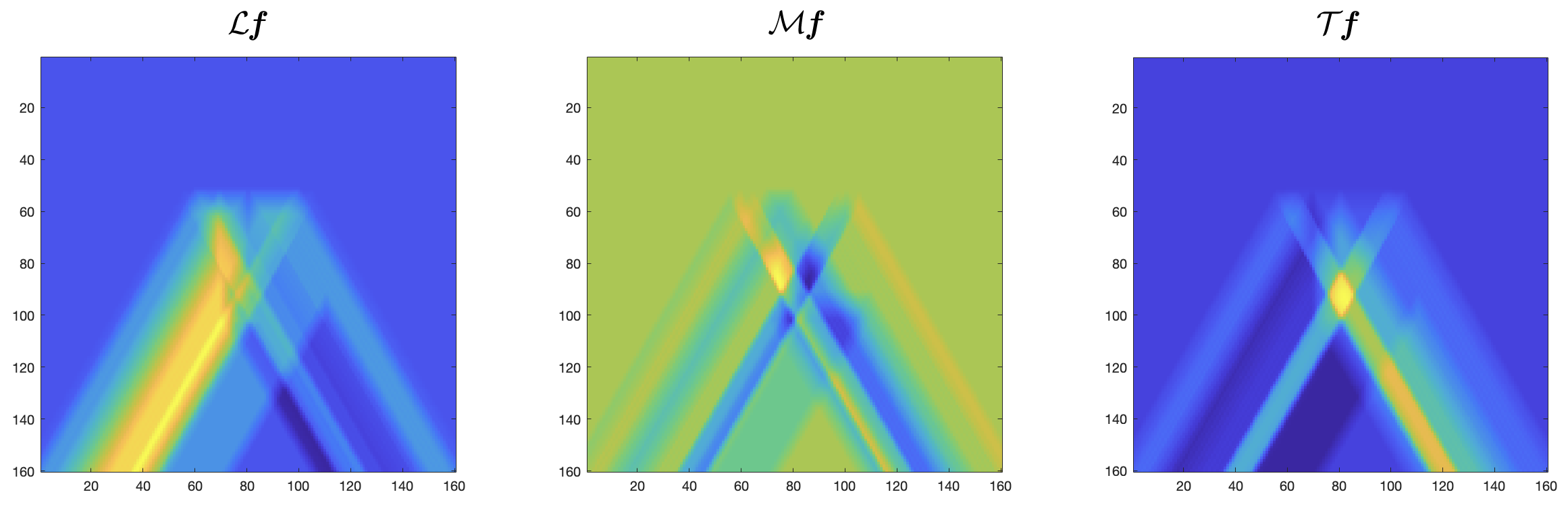
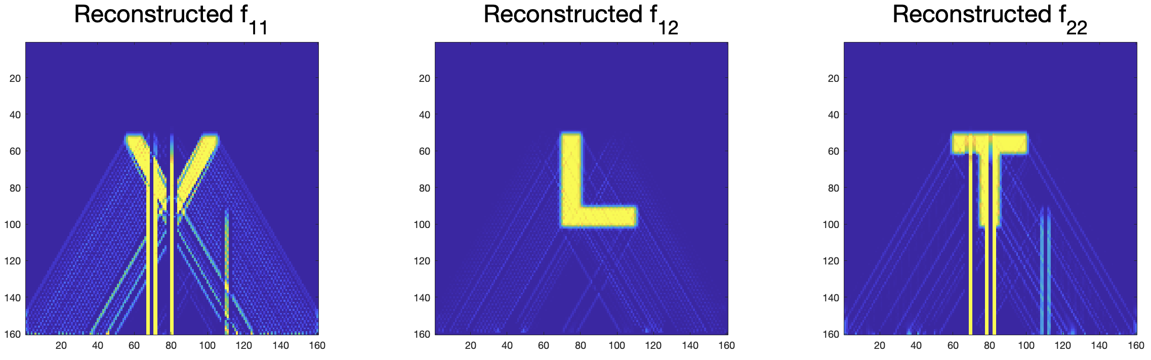
Figure 18: Components of f(Row 1), longitudinal ($\mathcal{L}\textbf{{f}}$), mixed($\mathcal{M}\textbf{{f}}$) and transverse ($\mathcal{T}\textbf{{f}}$) V-line transforms of f (Row 2), reconstructed components of f when $\textbf{{u}}=(\cos{\pi/3},\sin{\pi/3})$ using formulas (47),(48),(49) (Row 3).

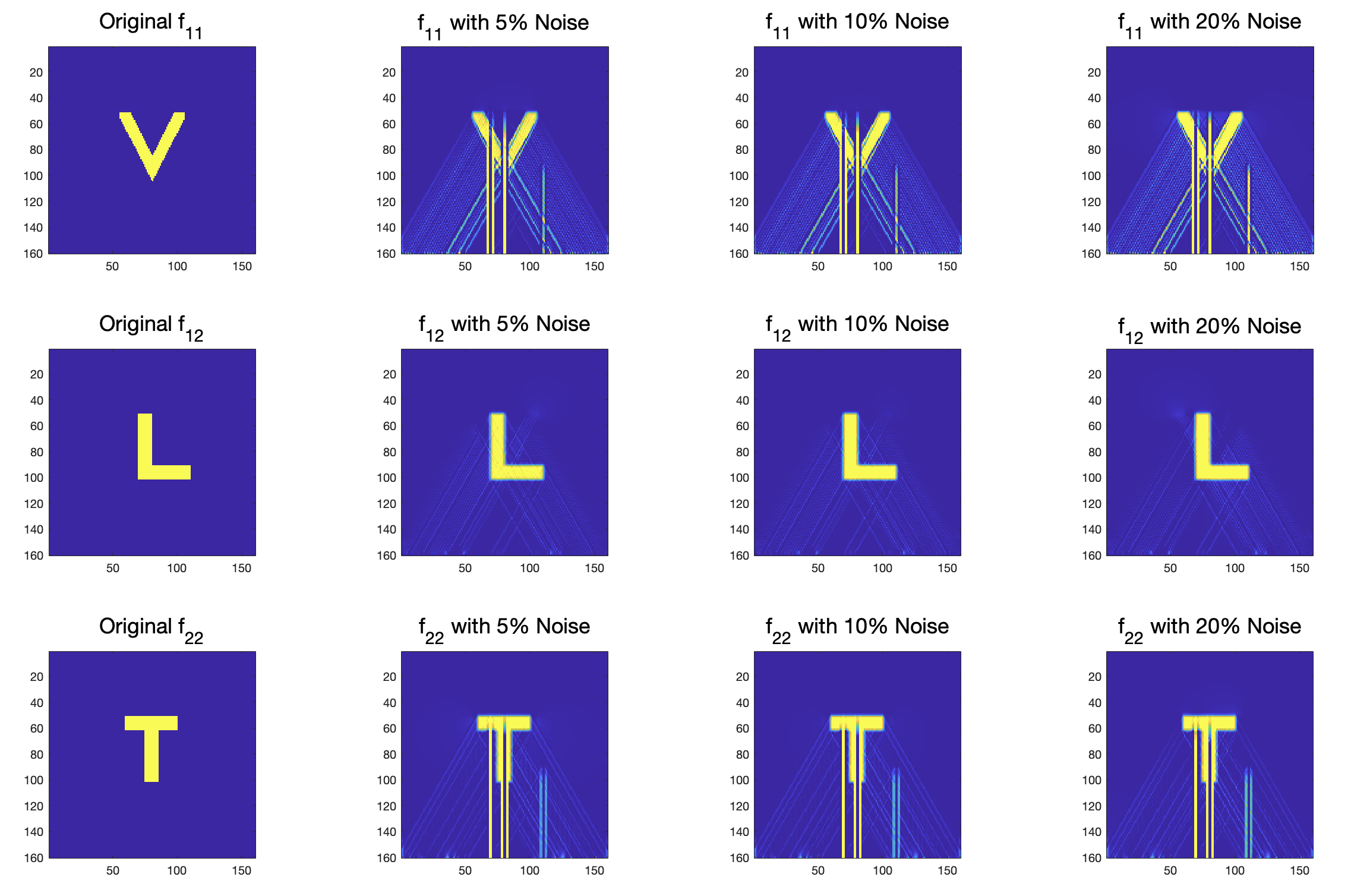
Figure 19: Reconstruction of f from $\mathcal{L}\textbf{{f}},\mathcal{M}\textbf{{f}},\mathcal{T}\textbf{{f}}$ when $\textbf{{u}}=(\cos{\pi/3,\sin{\pi/3}})$ with $5\%,10\%$ and $20\%$ noise

f	No noise	$5\%$ Noise	$10\%$ Noise	$20\%$ Noise
$f_{11}$	321.77%	293.14%	338.85%	450.29%
$f_{12}$	16.26%	16.29%	18.79%	24.92%
$f_{22}$	234.58%	262.40%	273.35%	257.46%

Table 11: Relative errors of reconstruction of $f_{11},f_{12},f_{22}$ from $\mathcal{L}\textbf{{f}},\mathcal{M}\textbf{{f}}$ and $\mathcal{T}\textbf{{f}}$ when $\textbf{{u}}=(\cos{\pi/3,\sin{\pi/3}})$

4.3 Recovery of tensor field f from moments

This subsection is devoted to the full recovery of f from various combinations of its V-line transforms and its first moments. The reconstruction of the unknown tensor field can be obtained from different combinations, such as $\mathcal{L}\textbf{{f}},\mathcal{L}^{1}\textbf{{f}},\mathcal{T}\textbf{{f}}$, or $\mathcal{T}\textbf{{f}},\mathcal{T}^{1}\textbf{{f}},\mathcal{L}\textbf{{f}}$, or $\mathcal{M}\textbf{{f}},\mathcal{M}^{1}\textbf{{f}},\mathcal{L}\textbf{{f}}$ or $\mathcal{M}\textbf{{f}},\mathcal{M}^{1}\textbf{{f}},\mathcal{T}\textbf{{f}}$, $\mathcal{L}\textbf{{f}},\mathcal{L}^{1}\textbf{{f}},\mathcal{M}\textbf{{f}}$, or $\mathcal{T}\textbf{{f}},\mathcal{T}^{1}\textbf{{f}},\mathcal{M}\textbf{{f}}$. Here, we discuss only two combinations $\mathcal{L}\textbf{{f}},\mathcal{L}^{1}\textbf{{f}},\mathcal{T}\textbf{{f}}$ and $\mathcal{L}\textbf{{f}},\mathcal{L}^{1}\textbf{{f}},\mathcal{M}\textbf{{f}}$ as other combinations are similar to one of these cases. More specifically, we discuss the recovery of f from $\mathcal{L}\textbf{{f}},\mathcal{L}^{1}\textbf{{f}},\mathcal{T}\textbf{{f}}$ when $\textbf{{u}}=(\cos{\pi/3},\sin{\pi/3})$ and from $\mathcal{L}\textbf{{f}},\mathcal{L}^{1}\textbf{{f}},\mathcal{M}\textbf{{f}}$ when $\textbf{{u}}=(\cos{\pi/4},\sin{\pi/4}).$

Theorem 4.

If $u_{1}\neq u_{2}$, then each component of $\textbf{{f}}\in C_{c}^{2}\left(S^{2};D_{1}\right)$ can be recovered from $\mathcal{L}\textbf{{f}}$, $\mathcal{L}^{1}\textbf{{f}}$, and $\mathcal{T}\textbf{{f}}$ by

$$f_{11}(\textbf{{x}}) =\frac{1}{(u_{2}^{2}-u_{1}^{2})}\left[\frac{1}{2}\left(D_{\textbf{{u}}}D_{\textbf{{v}}}\mathcal{L}^{1}\textbf{{f}}(\textbf{{x}})+(D_{\textbf{{u}}}+D_{\textbf{{v}}})\mathcal{L}\textbf{{f}}(\textbf{{x}})\right)+\frac{u_{2}}{2}D_{\textbf{{u}}}D_{\textbf{{v}}}\mathcal{X}_{\textbf{{e}}_{2}}\left(\mathcal{L}\textbf{{f}}+\mathcal{T}\textbf{{f}}\right)(\textbf{{x}})\right]$$ (50)

$$f_{12}(\textbf{{x}}) =\frac{1}{4u_{1}^{2}}\partial_{x_{2}}\mathcal{X}_{\textbf{{e}}_{1}}\left[\left(\frac{D_{\textbf{{u}}}D_{\textbf{{v}}}\mathcal{X}_{\textbf{{e}}_{2}}}{u_{2}}+D_{\textbf{{u}}}+D_{\textbf{{v}}}\right)\mathcal{L}\textbf{{f}}(\textbf{{x}})+D_{\textbf{{u}}}D_{\textbf{{v}}}\mathcal{L}^{1}\textbf{{f}}(\textbf{{x}})\right]$$ (51)

$$f_{22}(\textbf{{x}}) =\frac{1}{(u_{1}^{2}-u_{2}^{2})}\left[\frac{1}{2}\left(D_{\textbf{{u}}}D_{\textbf{{v}}}\mathcal{L}^{1}\textbf{{f}}(\textbf{{x}})+(D_{\textbf{{u}}}+D_{\textbf{{v}}})\mathcal{L}\textbf{{f}}(\textbf{{x}})\right)+\frac{u_{1}^{2}}{2u_{2}}D_{\textbf{{u}}}D_{\textbf{{v}}}\mathcal{X}_{\textbf{{e}}_{2}}\left(\mathcal{L}\textbf{{f}}+\mathcal{T}\textbf{{f}}\right)(\textbf{{x}})\right]$$ (52)

Theorem 5.

The components of a tensor field $\textbf{{f}}\in C_{c}^{2}\left(S^{2};D_{1}\right)$ can be recovered from $\mathcal{L}\textbf{{f}}$, $\mathcal{L}^{1}\textbf{{f}}$, and $\mathcal{M}\textbf{{f}}$ by

$$f_{12}(\textbf{{x}}) =\frac{1}{4u_{1}^{2}}\partial_{x_{2}}\mathcal{X}_{\textbf{{e}}_{1}}\left[\left(\frac{D_{\textbf{{u}}}D_{\textbf{{v}}}\mathcal{X}_{\textbf{{e}}_{2}}}{u_{2}}+D_{\textbf{{u}}}+D_{\textbf{{v}}}\right)\mathcal{L}\textbf{{f}}(\textbf{{x}})+D_{\textbf{{u}}}D_{\textbf{{v}}}\mathcal{L}^{1}\textbf{{f}}(\textbf{{x}})\right]$$ (53)

$$f_{11}(\textbf{{x}}) =-\frac{1}{2}\left(D_{\textbf{{u}}}D_{\textbf{{v}}}\mathcal{L}^{1}\textbf{{f}}(\textbf{{x}})+(D_{\textbf{{u}}}+D_{\textbf{{v}}})\mathcal{L}\textbf{{f}}(\textbf{{x}})\right)+\frac{u_{2}}{2u_{1}^{2}}D_{\textbf{{u}}}D_{\textbf{{v}}}\mathcal{X}_{-\textbf{{e}}_{1}}\left[(u_{1}^{2}-u_{2}^{2})\mathcal{V}(f_{12})(\textbf{{x}})-\mathcal{M}\textbf{{f}}(\textbf{{x}})\right]$$ (54)

$$f_{22}(\textbf{{x}}) =-\frac{1}{2}\left(D_{\textbf{{u}}}D_{\textbf{{v}}}\mathcal{L}^{1}\textbf{{f}}(\textbf{{x}})+(D_{\textbf{{u}}}+D_{\textbf{{v}}})\mathcal{L}\textbf{{f}}(\textbf{{x}})\right)-\frac{1}{2u_{2}}D_{\textbf{{u}}}D_{\textbf{{v}}}\mathcal{X}_{-\textbf{{e}}_{1}}\left[(u_{1}^{2}-u_{2}^{2})\mathcal{V}(f_{12})(\textbf{{x}})-\mathcal{M}\textbf{{f}}(\textbf{{x}})\right]$$ (55)

Remark 7.

When $u_{1}\neq u_{2},$ to recover $f_{11},f_{22}$ using Theorem (4), we don’t need the information of reconstructed $f_{12}$, whereas if we use Theorem (5) we have to use the knowledge of reconstructed $f_{12}$ to recover $f_{11}$ and $f_{22}.$ But this reconstructed $f_{12}$ possesses artifacts that transcend to the next step in the recovery of $f_{11}$ and $f_{22}$. Thus, for $u_{1}\neq u_{2}$ case, to recover $\textbf{{f}},$ Theorem (4) is better than Theorem (5).

The Figures 20,22 generated as a result of implementing formulas (50), (51) and (52) for the smooth phantom and non-smooth phantom, respectively. Further, Figures 21, 23 showed the effect of noise on the recovery for both types of phantoms.

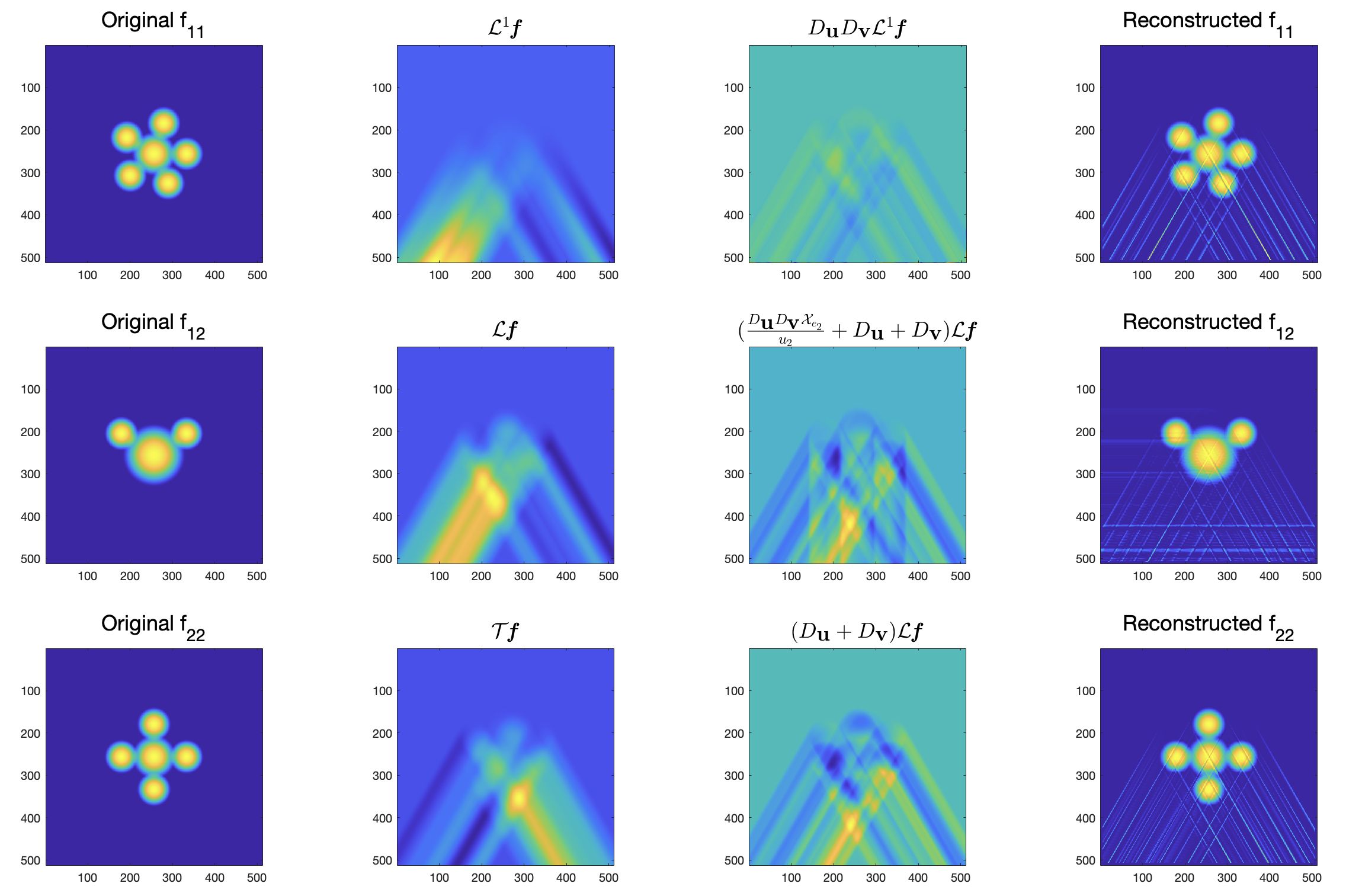
Figure 20: (Column-1) Components of f, (Column-2) first moment longitudinal ($\mathcal{L}^{1}\textbf{{f}}$), longitudinal ($\mathcal{L}\textbf{{f}}$) and transverse ($\mathcal{T}\textbf{{f}}$) V-line transforms of f, (Column-3) $D_{\textbf{{u}}}D_{\textbf{{v}}}\mathcal{L}^{1}\textbf{{f}}$, $\left(\frac{D_{\textbf{{u}}}D_{\textbf{{v}}}\mathcal{X}_{\textbf{{e}}_{2}}}{u_{2}}+D_{\textbf{{u}}}+D_{\textbf{{v}}}\right)\mathcal{L}\textbf{{f}}$ and $(D_{\textbf{{u}}}+D_{\textbf{{v}}})\mathcal{L}\textbf{{f}}$, (Column-4) reconstructed components of f when $\textbf{{u}}=(\cos{\pi/3},\sin{\pi/3})$ using formulas (50),(51),(52)

..

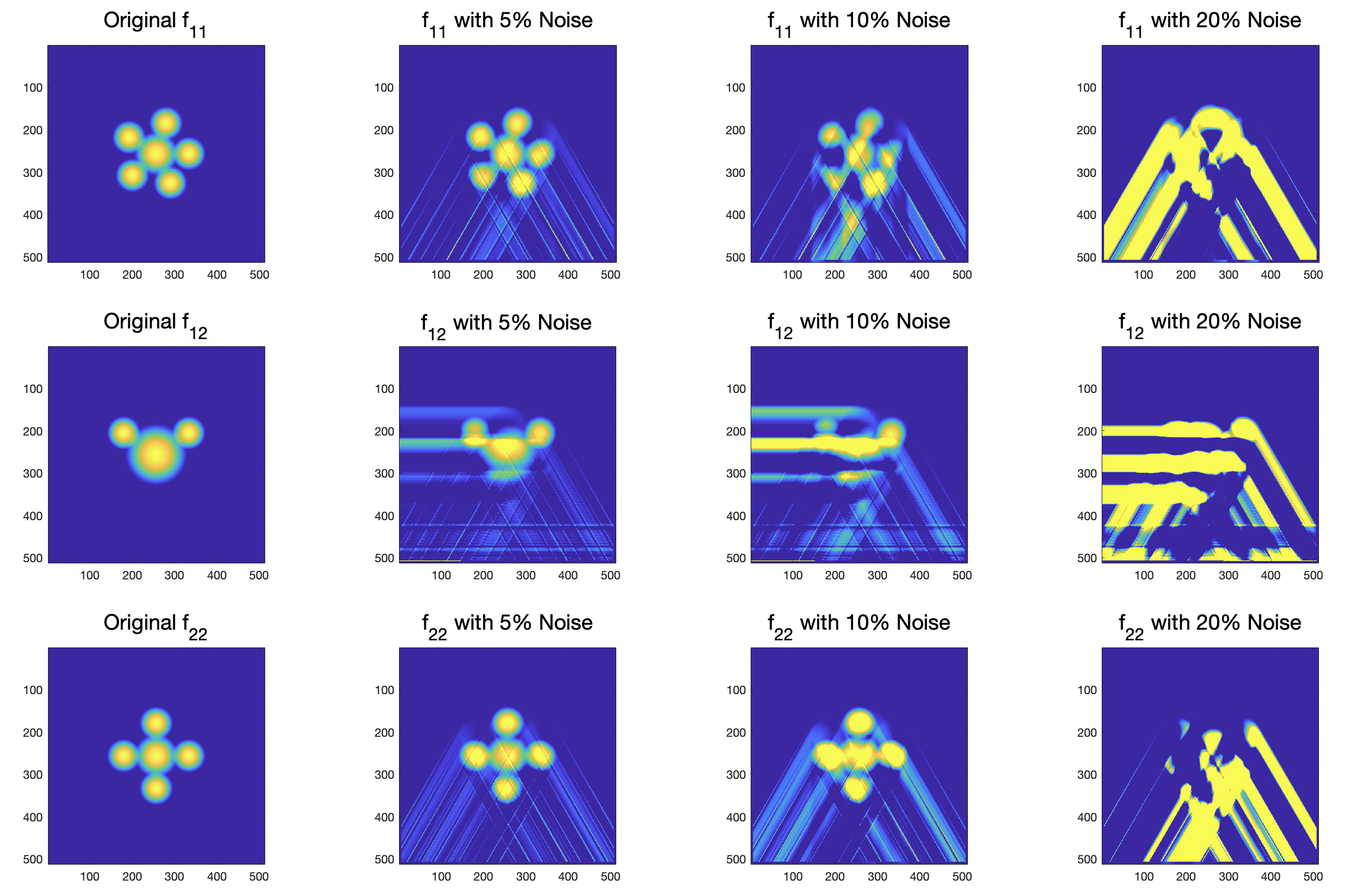
Figure 21: Reconstruction of f from $\mathcal{L}\textbf{{f}},\mathcal{L}^{1}\textbf{{f}},\mathcal{T}\textbf{{f}}$ when $\textbf{{u}}=(\cos{\pi/3,\sin{\pi/3}})$ with $5\%,10\%$ and $20\%$ noise

.

f	No noise	$5\%$ Noise	$10\%$ Noise	$20\%$ Noise
$f_{11}$	13.77%	17.29%	61.49%	428.98%
$f_{12}$	806.32%	833.58%	990.84%	2404.38%
$f_{22}$	14.10%	18.43%	63.49%	445.50%

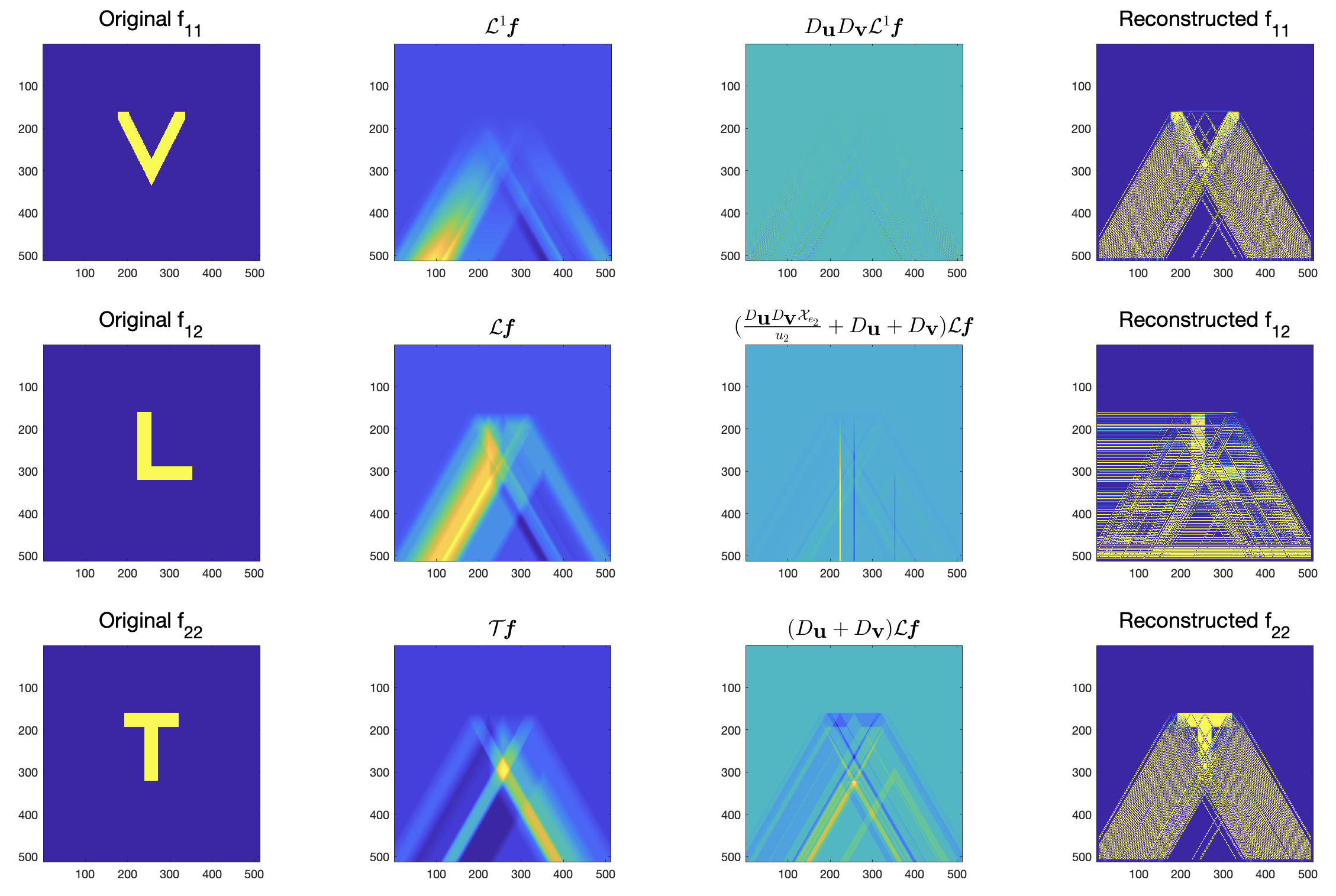
Figure 22: (Column-1) Components of f, (Column-2) first moment longitudinal ($\mathcal{L}^{1}\textbf{{f}}$), longitudinal ($\mathcal{L}\textbf{{f}}$) and transverse ($\mathcal{T}\textbf{{f}}$) V-line transforms of f, (Column-3) $D_{\textbf{{u}}}D_{\textbf{{v}}}\mathcal{L}^{1}\textbf{{f}}$, $\left(\frac{D_{\textbf{{u}}}D_{\textbf{{v}}}\mathcal{X}_{\textbf{{e}}_{2}}}{u_{2}}+D_{\textbf{{u}}}+D_{\textbf{{v}}}\right)\mathcal{L}\textbf{{f}}$ and $(D_{\textbf{{u}}}+D_{\textbf{{v}}})\mathcal{L}\textbf{{f}}$, (Column-4) reconstructed components of f when $\textbf{{u}}=(\cos{\pi/3},\sin{\pi/3})$ using formulas (50),(51),(52)

.

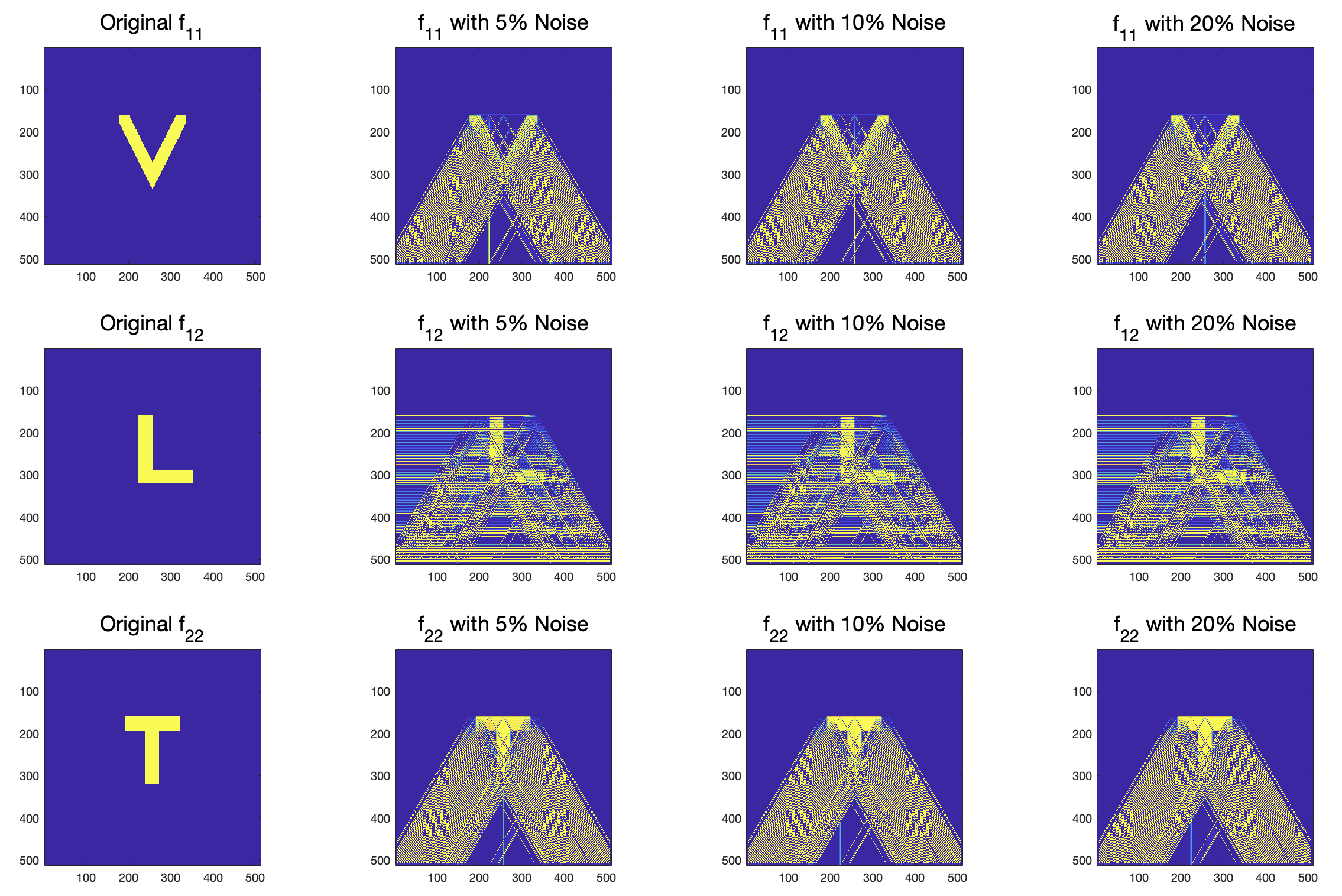
Figure 23: Reconstruction of f from $\mathcal{L}\textbf{{f}},\mathcal{L}^{1}\textbf{{f}},\mathcal{T}\textbf{{f}}$ when $\textbf{{u}}=(\cos{\pi/3,\sin{\pi/3}})$ with $5\%,10\%$ and $20\%$ noise

.

f	No noise	$5\%$ Noise	$10\%$ Noise	$20\%$ Noise
$f_{11}$	4009.19%	4036.22%	4215.82%	4218.84%
$f_{12}$	2408.93%	2422.88%	2534.95%	2532.71%
$f_{22}$	3041.98 %	3062.53%	3198.72%	3201.04%

Next, we consider recovery of f from the combination $\mathcal{L}\textbf{{f}},\mathcal{L}^{1}\textbf{{f}}$ and $\mathcal{M}\textbf{{f}}.$ In Figures 24 ,26, the inversion formulas (53), (54), and (55) to generate $f_{12}$, $f_{11}$, and $f_{22}$ respectively for the smooth and non-smooth phantoms. Figures 25 and 27 show the reconstructions after adding different levels of noise for smooth and non-smooth phantoms, respectively.

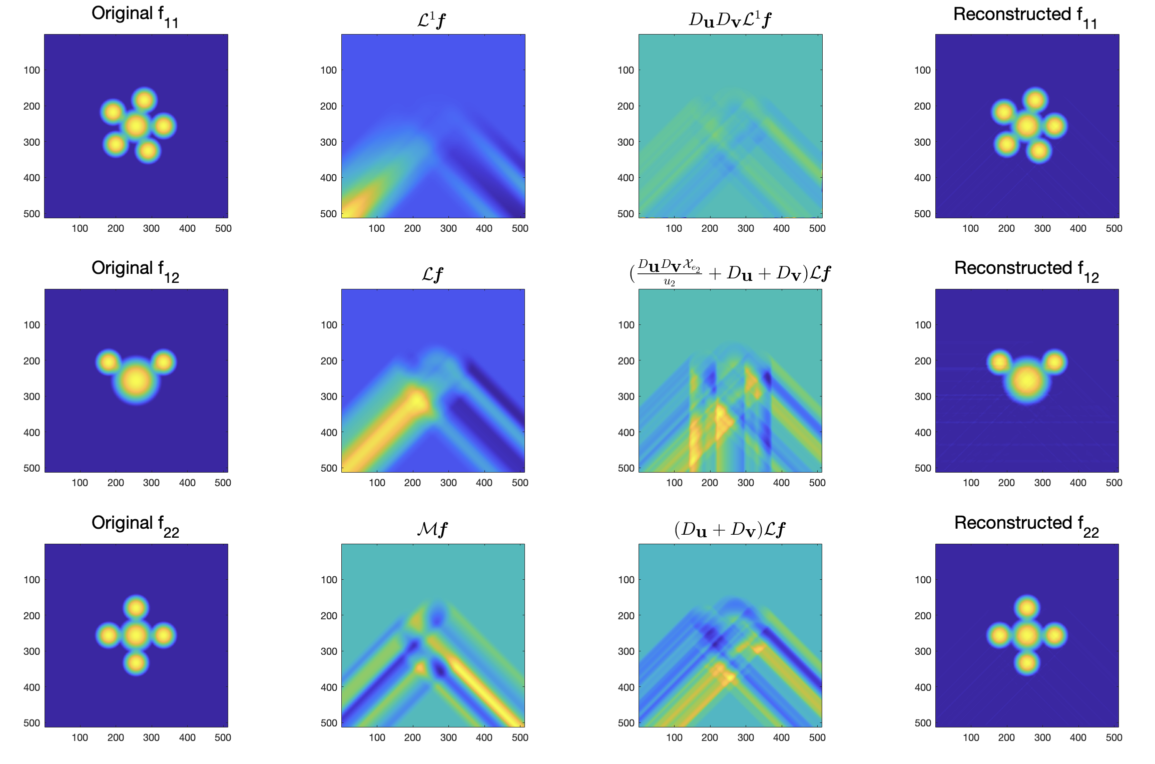
Figure 24: (Column-1) Components of f, (Column-2) first moment longitudinal ($\mathcal{L}^{1}\textbf{{f}}$), longitudinal ($\mathcal{L}\textbf{{f}}$) and mixed ($\mathcal{M}\textbf{{f}}$) V-line transforms of f, (Column-3) $D_{\textbf{{u}}}D_{\textbf{{v}}}\mathcal{L}^{1}\textbf{{f}}$, $\left(\frac{D_{\textbf{{u}}}D_{\textbf{{v}}}\mathcal{X}_{\textbf{{e}}_{2}}}{u_{2}}+D_{\textbf{{u}}}+D_{\textbf{{v}}}\right)\mathcal{L}\textbf{{f}}$ and $(D_{\textbf{{u}}}+D_{\textbf{{v}}})\mathcal{L}\textbf{{f}}$, (Column-4) reconstructed components of f when $\textbf{{u}}=(\cos{\pi/4},\sin{\pi/4})$ using formulas (53),(54),(55)

.

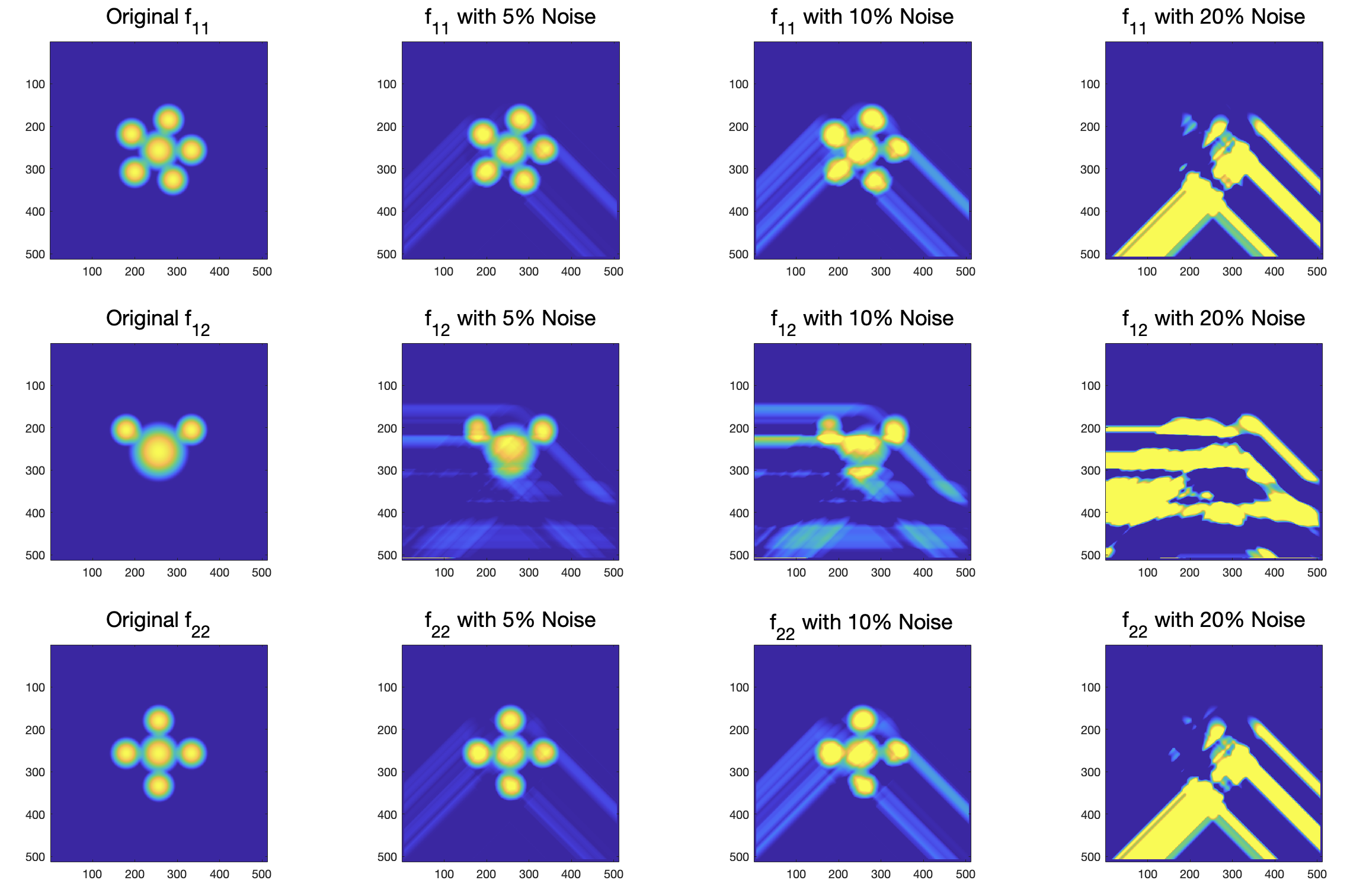
Figure 25: Reconstruction of f from $\mathcal{L}\textbf{{f}},\mathcal{L}^{1}\textbf{{f}},\mathcal{M}\textbf{{f}}$ when $\textbf{{u}}=(\cos{\pi/4,\sin{\pi/4}})$ with $5\%,10\%$ and $20\%$ noise

.

f	No noise	$5\%$ Noise	$10\%$ Noise	$20\%$ Noise
$f_{11}$	0.68%	11.72%	37.44%	273.99%
$f_{12}$	803.03%	840.92%	1008.68%	1325.82%
$f_{22}$	0.70%	11.70%	38.17%	278.72%

.

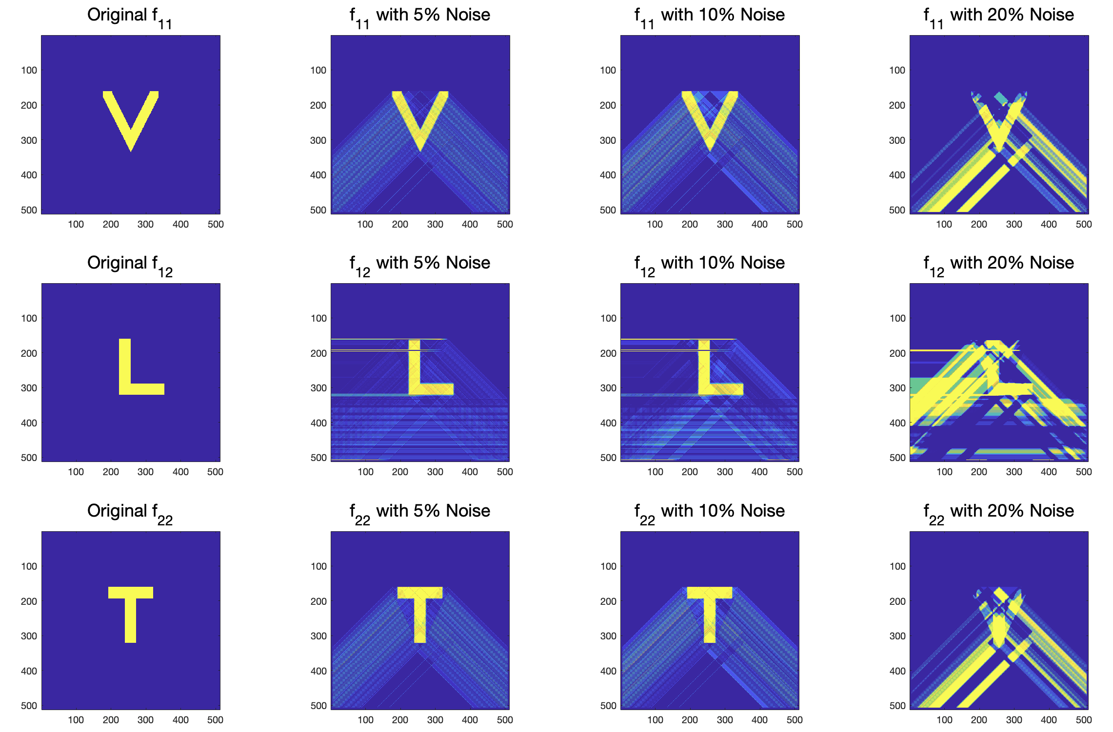
Figure 27: Reconstruction of f from $\mathcal{L}\textbf{{f}},\mathcal{L}^{1}\textbf{{f}},\mathcal{M}\textbf{{f}}$ when $\textbf{{u}}=(\cos{\pi/4,\sin{\pi/4}})$ with $5\%,10\%$ and $20\%$ noise

f	No noise	$5\%$ Noise	$10\%$ Noise	$20\%$ Noise
$f_{11}$	81.83%	82.69%	92.73%	204.12%
$f_{12}$	857.81%	883.65%	1026.22%	1378.59%
$f_{22}$	62.14%	62.80%	70.42%	156.51%

4.4 Implementation for the star transform

Before starting our discussion about the star transform of symmetric 2-tensor fields, let us quickly recall the definition of the star transform. For $\textbf{{f}}\in C_{c}^{2}\left(S^{2};\mathbb{R}^{2}\right)$, and let $\boldsymbol{\gamma}_{1},\boldsymbol{\gamma}_{2},...,\boldsymbol{\gamma}_{m}$ be distinct unit vectors in $\mathbb{R}^{2}$. The star transform of f is defined as

$$\mathcal{S}\textbf{{f}} =\sum_{i=1}^{m}c_{i}{\mathcal{X}}_{{\boldsymbol{\gamma}}_{i}}\begin{bmatrix}\textbf{{f}}\cdot{{\boldsymbol{\gamma}}_{i}}^{2}\\ \textbf{{f}}\cdot{{\boldsymbol{\gamma}}_{i}\odot{\boldsymbol{\gamma}}_{i}^{\perp}}\\ \textbf{{f}}\cdot({\boldsymbol{\gamma}}_{i}^{\perp})^{2}\end{bmatrix},$$

where $c_{1},c_{2},\dots,c_{m}$ are non-zero constants in $\mathbb{R}$.

Definition 5.

A star transform $\mathcal{S}$ is called symmetric if $m=2k$ for some $k\in\mathbb{N}$ and (after possible index rearrangement) $\boldsymbol{\gamma}_{i+k}=-\boldsymbol{\gamma}_{i}$ with $c_{i+k}=c_{i}$ for all $i=1,2,\dots,k.$

Definition 6.

Consider the star transform $\mathcal{S}\textbf{{f}}$ of a symmetric 2-tensor field f with branches along directions $\boldsymbol{\gamma}_{1},\boldsymbol{\gamma}_{2},...,\boldsymbol{\gamma}_{m}$. We call

$$\mathcal{Z}_{1}=\cup_{i=1}^{m}\{\boldsymbol{\xi}:\boldsymbol{\xi}\cdot{\boldsymbol{\gamma}}_{i}=0\}$$

the set of singular directions of type 1 for $\mathcal{S}$.

Now, let us define three vectors in $\mathbb{R}^{3}$, which will be important for further calculations. For $\boldsymbol{\xi}\in\mathbb{S}^{1}\setminus\mathcal{Z}_{1}$, we define

$$\boldsymbol{\gamma}(\boldsymbol{\xi})=-\sum_{i=1}^{m}\frac{c_{i}{\boldsymbol{\gamma}}_{i}^{2}}{\boldsymbol{\xi}\cdot{\boldsymbol{\gamma}}_{i}},\qquad\boldsymbol{\gamma}^{\dagger}(\boldsymbol{\xi})=-\sum_{i=1}^{m}\frac{c_{i}{\boldsymbol{\gamma}}_{i}\odot\boldsymbol{\gamma}_{i}^{\perp}}{\boldsymbol{\xi}\cdot{\boldsymbol{\gamma}}_{i}},\qquad\boldsymbol{\gamma}^{\perp}(\boldsymbol{\xi})=-\sum_{i=1}^{m}\frac{c_{i}({\boldsymbol{\gamma}_{i}}^{\perp})^{2}}{\boldsymbol{\xi}\cdot{\boldsymbol{\gamma}}_{i}}.$$ (56)

Definition 7.

We call

$$\mathcal{Z}_{2}=\left\{\boldsymbol{\xi}:\boldsymbol{\gamma}^{\dagger}(\boldsymbol{\xi})=0\right\}\ \bigcup\ \left\{\boldsymbol{\xi}:\sum_{i=1}^{m}\frac{c_{i}}{\boldsymbol{\xi}\cdot\boldsymbol{\gamma}_{i}}=0\right\}$$

the set of singular directions of type 2 for $\mathcal{S}$.

Theorem 6.

Let $\textbf{{f}}\in C_{c}^{2}\left(S^{2};D_{1}\right)$, and $\boldsymbol{\gamma}_{1},\boldsymbol{\gamma}_{2},\dots,\boldsymbol{\gamma}_{m}$ be the branch directions of the star transform. Let

$$\mathcal{Q}(\boldsymbol{\xi})=\begin{bmatrix}{\boldsymbol{\gamma}}(\boldsymbol{\xi})\\ {\boldsymbol{\gamma}}^{{\dagger}}(\boldsymbol{\xi})\\ {\boldsymbol{\gamma}}^{\perp}(\boldsymbol{\xi})\end{bmatrix}.$$

Then for any $\boldsymbol{\xi}\in\mathbb{S}^{1}\setminus(\mathcal{Z}_{1}\cup\mathcal{Z}_{2})$ and any $s\in\mathbb{R}$ we have

$$\left[\mathcal{Q}(\boldsymbol{\xi})\right]^{-1}\frac{d}{ds}\mathcal{R}({\mathcal{S}}\textbf{{f}})(\boldsymbol{\xi},s)=\mathcal{R}\textbf{{f}}(\boldsymbol{\xi},s)$$ (57)

where $\mathcal{R}\textbf{{f}}$ is the component-wise Radon transform of f.

To reconstruct numerically the tensor from its star transform, we considered the brunches along $\boldsymbol{\gamma}_{i}=(\cos\phi_{i},\sin\phi_{i})$ where $\phi_{1}=0,\phi_{2}=2\pi/3,\phi_{3}=4\pi/3$ with weights $c_{i}=1$ for $i=1,2,3$.The reconstruction is performed by using the following steps:

• Calculate $\mathcal{X}_{\boldsymbol{\gamma}_{i}}(\textbf{{f}}\cdot{{\boldsymbol{\gamma}}_{i}}^{2}),\mathcal{X}_{\boldsymbol{\gamma}_{i}}(\textbf{{f}}\cdot{{\boldsymbol{\gamma}}_{i}\odot{\boldsymbol{\gamma}}_{i}^{\perp}}),\mathcal{X}_{\boldsymbol{\gamma}_{i}}(\textbf{{f}}\cdot({\boldsymbol{\gamma}}_{i}^{\perp})^{2})$. Then, combining these according to the formula, we generate the data for $\mathcal{S}\textbf{{f}}.$

• Using the radon function we generate data for $\mathcal{R}(\mathcal{S}\textbf{{f}})(\boldsymbol{\xi},s)$ and then calculate $\frac{d}{ds}\mathcal{R}({\mathcal{S}}\textbf{{f}})(\boldsymbol{\xi},s).$

• Next for each value of $\boldsymbol{\xi}$ we compute $[\mathcal{Q}(\boldsymbol{\xi})]^{-1}$ and then multiply with $\frac{d}{ds}\mathcal{R}({\mathcal{S}}\textbf{{f}})(\boldsymbol{\xi},s).$

• Finally, using iradon to $\displaystyle\left[\mathcal{Q}(\boldsymbol{\xi})\right]^{-1}\frac{d}{ds}\mathcal{R}({\mathcal{S}}\textbf{{f}})(\boldsymbol{\xi},s)$, we recover $\textbf{{f}}.$

In Figure 28, we show the reconstruction obtained by the algorithm discussed above for the non-smooth phantom, and Figure 29 deals the corresponding reconstruction in the presence of noise.

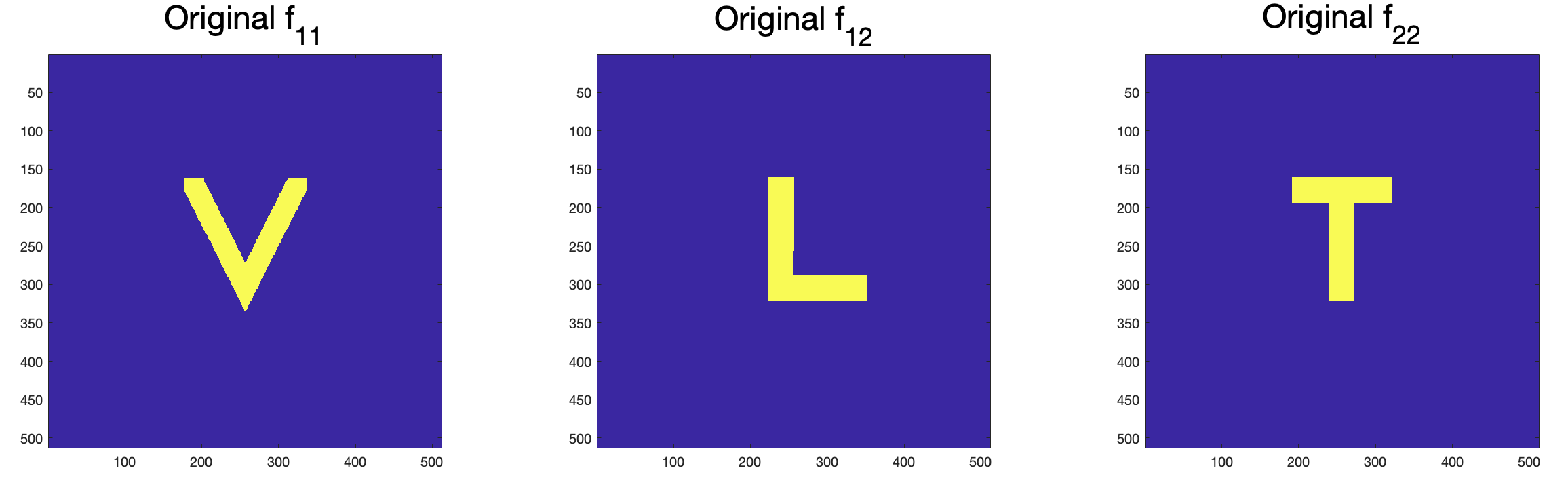
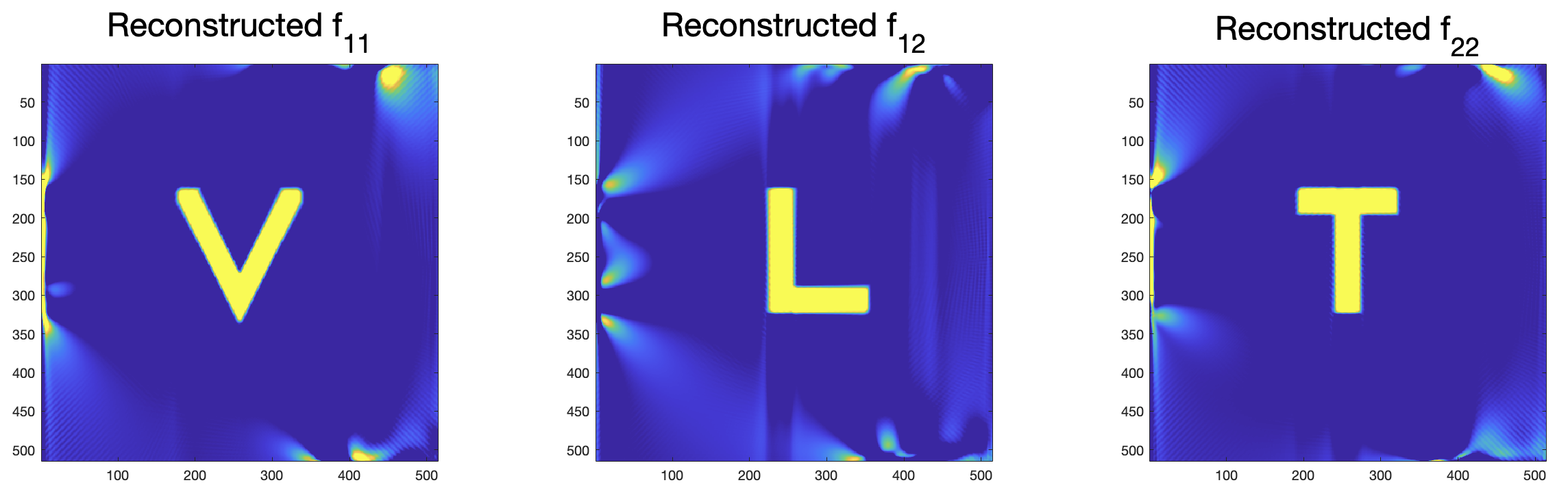
Figure 28: Components of f(Row 1), longitudinal (LCS), mixed(MCS) and transverse (TCS) components of $\mathcal{S}\textbf{{f}}$ (Row 2), reconstructed components of f using formula (57) (Row 3).

Figure 29: Reconstruction of f from $\mathcal{S}\textbf{{f}}$ with $5\%,10\%$ and $20\%$ noise

f	No noise	$5\%$ Noise	$10\%$ Noise	$20\%$ Noise
$f_{11}$	114.01%	114.72%	128.88%	175.17%
$f_{12}$	92.41%	96.36%	96.81%	115.22%
$f_{22}$	95.56%	96.02%	109.25%	139.61%

Table 12: Relative errors of the reconstruction of f from $\mathcal{S}\textbf{{f}}$

5 Acknowledgements

GA was partially supported by the NIH grant U01-EB029826. RM was partially supported by SERB SRG grant No. SRG/2022/000947. IZ was supported by the Prime Minister’s Research Fellowship from the Government of India.

References

- [1] Gaik Ambartsoumian. Inversion of the V-line Radon transform in a disc and its applications in imaging. Computers & Mathematics with Applications, 64(3):260–265, 2012.
- [2] Gaik Ambartsoumian. V-line and conical Radon transforms with applications in imaging. In Ronny Ramlau and Otmar Scherzer, editors, The Radon Transform: The First 100 Years and Beyond, pages 143–168. De Gruyter, Berlin, Boston, 2019.
- [3] Gaik Ambartsoumian. Generalized Radon Transforms and Imaging by Scattered Particles: Broken Rays, Cones, and Stars in Tomography. World Scientific, 2023.
- [4] Gaik Ambartsoumian and Mohammad J. Latifi. The V-line transform with some generalizations and cone differentiation. Inverse Problems, 35(3):034003, 2019.
- [5] Gaik Ambartsoumian and Mohammad J. Latifi. Inversion and symmetries of the star transform. The Journal of Geometric Analysis, 31(11):11270–11291, 2021.
- [6] Gaik Ambartsoumian, Mohammad J. Latifi, and Rohit K. Mishra. Generalized V-line transforms in 2D vector tomography. Inverse Problems, 36(10):104002, 2020.
- [7] Gaik Ambartsoumian, Mohammad J. Latifi, and Rohit K. Mishra. Numerical implementation of generalized V-line transforms on 2D vector fields and their inversions. SIAM Journal on Imaging Sciences, 17(1):595–631, 2024.
- [8] Gaik Ambartsoumian, Rohit K. Mishra, and Indrani Zamindar. V-line 2-tensor tomography in the plane. Inverse Problems, 40(3):035003, 2024.
- [9] Gaik Ambartsoumian and Sunghwan Moon. A series formula for inversion of the V-line Radon transform in a disc. Computers & Mathematics with Applications, 66(9):1567–1572, 2013.
- [10] Gaik Ambartsoumian and Souvik Roy. Numerical inversion of a broken ray transform arising in single scattering optical tomography. IEEE Transactions on Computational Imaging, 2(2):166–173, 2016.
- [11] Roman Basko, Gengsheng L. Zeng, and Grant T. Gullberg. Analytical reconstruction formula for one-dimensional Compton camera. IEEE Transactions on Nuclear Science, 44(3):1342–1346, Jun 1997.
- [12] Roman Basko, Gengsheng L. Zeng, and Grant T. Gullberg. Fully three dimensional image reconstruction from “V”-projections acquired by Compton camera with three vertex electronic collimation. In 1997 IEEE Nuclear Science Symposium Conference Record, volume 2, pages 1077–1081, Nov 1997.
- [13] Rahul Bhardwaj, Rohit K. Mishra, and Manmohan Vashisth. Inversion of generalized V-line transforms of vector fields in . Preprint, arXiv:2404.12479, 2024.
- [14] Evgeny Yu. Derevtsov and Ivan E. Svetov. Tomography of tensor fields in the plane. Eurasian Journal of Mathematical and Computer Applications, 3(2):24–68, 2015.
- [15] Dale R. Durran. Numerical Methods For Wave Equations In Geophysical Fluid Dynamics, volume 32. Springer Science & Business Media, 2013.
- [16] Lucia Florescu, Vadim A. Markel, and John C. Schotland. Single-scattering optical tomography: Simultaneous reconstruction of scattering and absorption. Physical Review E, 81:016602, Jan 2010.
- [17] Lucia Florescu, Vadim A. Markel, and John C. Schotland. Inversion formulas for the broken-ray Radon transform. Inverse Problems, 27(2):025002, 2011.
- [18] Lucia Florescu, Vadim A Markel, and John C Schotland. Nonreciprocal broken ray transforms with applications to fluorescence imaging. Inverse Problems, 34(9):094002, 2018.
- [19] Lucia Florescu, John C. Schotland, and Vadim A. Markel. Single-scattering optical tomography. Physical Review E, 79:036607, Mar 2009.
- [20] Rim Gouia-Zarrad. Analytical reconstruction formula for -dimensional conical Radon transform. Computers & Mathematics with Applications, 68(9):1016–1023, 2014.
- [21] Rim Gouia-Zarrad and Gaik Ambartsoumian. Exact inversion of the conical Radon transform with a fixed opening angle. Inverse Problems, 30(4):045007, 2014.
- [22] Joonas Ilmavirta and Gabriel P. Paternain. Broken ray tensor tomography with one reflecting obstacle. Communications in Analysis and Geometry, 30(6):1269–1300, 2022.
- [23] Joonas Ilmavirta and Mikko Salo. Broken ray transform on a Riemann surface with a convex obstacle. Communications in Analysis and Geometry, 24(2):379–408, 2016.
- [24] Shubham R. Jathar, Manas Kar, and Jesse Railo. Broken ray transform for twisted geodesics on surfaces with a reflecting obstacle. Preprint, arXiv:2306.17604, 2024.
- [25] Alexander Katsevich and Roman Krylov. Broken ray transform: inversion and a range condition. Inverse Problems, 29(7):075008, 2013.
- [26] Roman Krylov and Alexander Katsevich. Inversion of the broken ray transform in the case of energy-dependent attenuation. Physics in Medicine & Biology, 60(11):4313, 2015.
- [27] Marcela Morvidone, Mai K. Nguyen, Tuong T. Truong, and Habib Zaidi. On the V-line Radon transform and its imaging applications. International Journal of Biomedical Imaging, 2010:208179, 2010.
- [28] Victor Palamodov. Reconstruction from cone integral transforms. Inverse Problems, 33(10):104001, 2017.
- [29] Gaël Rigaud, Rémi Régnier, Mai K. Nguyen, and Habib Zaidi. Combined modalities of Compton scattering tomography. IEEE Transactions on Nuclear Science, 60(3):1570–1577, 2013.
- [30] Vladimir A. Sharafutdinov. Integral Geometry of Tensor Fields. De Gruyter, Berlin, New York, 1994.
- [31] Brian Sherson. Some Results in Single-Scattering Tomography. PhD thesis, Oregon State University, 2015. PhD Advisor: D. Finch.
- [32] Tuong T. Truong and Mai K. Nguyen. On new V-line Radon transforms in and their inversion. Journal of Physics A: Mathematical and Theoretical, 44(7):075206, jan 2011.
- [33] Michael R Walker and Joseph A. O’Sullivan. Iterative algorithms for joint scatter and attenuation estimation from broken ray transform data. IEEE Transactions on Computational Imaging, 7:361–374, 2021.
- [34] Fan Zhao, John C. Schotland, and Vadim A. Markel. Inversion of the star transform. Inverse Problems, 30(10):105001, 2014.