Communication-Efficient Federated Learning with Adaptive Compression under Dynamic Bandwidth
Abstract
Federated learning can train models without directly providing local data to the server. However, the frequent updating of the local model brings the problem of large communication overhead. Recently, scholars have achieved the communication efficiency of federated learning mainly by model compression. But they ignore two problems: 1) network state of each client changes dynamically; 2) network state among clients is not the same. The clients with poor bandwidth update local model slowly, which leads to low efficiency. To address this challenge, we propose a communication-efficient federated learning algorithm with adaptive compression under dynamic bandwidth (called AdapComFL). Concretely, each client performs bandwidth awareness and bandwidth prediction. Then, each client adaptively compresses its local model via the improved sketch mechanism based on his predicted bandwidth. Further, the server aggregates sketched models with different sizes received. To verify the effectiveness of the proposed method, the experiments are based on real bandwidth data which are collected from the network topology we build, and benchmark datasets which are obtained from open repositories. We show the performance of AdapComFL algorithm, and compare it with existing algorithms. The experimental results show that our AdapComFL achieves more efficient communication as well as competitive accuracy compared to existing algorithms.
Index Terms:
Federated learning, communication efficiency, dynamic bandwidth, sketch.I Introduction
The development of communication technologies catalyzes diverse Internet of Things (IoT) scenarios, then the massive volumes of data generated by IoT clients can be fully employed to make people’s life more convenient, such as smart healthcare [1, 2, 3]. Generally, clients need transport their own data to third party for training, which exposes them to the risk of privacy leakage [4]. Fortunately, federated learning, which allows clients to participate in distributed training without move their raw data [5, 6, 7], bridges a light for machine learning with privacy protection. Compared with the framework of central machine learning, clients and the server require more rounds of communication in the framework of federated learning, which brings the communication overhead. In fact, communication cost becomes bottleneck of practical federated learning.
To achieve the communication efficiency of federated learning, there are two categories of approaches: (1) reducing the frequency of total communication by increasing the amount of local computation [1], Konečnỳ et al. [8] allow more local updates per communication round, Li et al. [9] dynamic adjusts the local calculation epoch of each client. These methods require powerful computing resources, and due to the emphasis on local training, the global model may have performance differences among clients. (2) reducing the volume of messages each round of communication. It uses different methods to compress local models, including stochastic sparsification [12, 11, 10, 13, 14], quantization [16, 21, 20, 12, 17, 18, 19, 15] and pruning [22, 23].
Stochastic sparsification mainly uses top-k sparsification method which filters the more important model parameters [11, 10]. For quantization including probability quantization and gradient quantization methods, the probability quantization characterizes the model parameters as extremum [12]. Gradient quantization considers model precision, which assigns different precisions according to the importance of the model parameter [17, 18, 19]. Moreover, some works combine quantization with stochastic sparsification [12, 13, 14]. For pruning, there are two main categories: structured pruning and unstructured pruning. Structured pruning reduces the model size by cutting out the unimportant parts of the model structure [22], while unstructured pruning maintains the original model size but cuts out unimportant model parameters [23]. The works mentioned above just focus on communication efficiency in federated learning but ignore privacy-preserving issues. Liu et al. [24] trade-off communication efficiency and privacy via the sketch compression method.
Remarkably, existing methods of achieving communication efficiency in federated learning ignore two problems. First, the network state of each client changes dynamically, as shown by changes in bandwidth. Second, bandwidth of clients is different. For clients with poor bandwidth, the server needs to delay the aggregation of the global model because these clients upload the local model slowly. Here, we address this challenge and propose a communication-efficient federated learning algorithm with adaptive compression under dynamic bandwidth, which is called AdapComFL. The workflow of AdapComFL algorithm is as follows in brief. (1) Clients carry out bandwidth awareness during local model training. (2) After training, clients predict bandwidth, and compress the model gradient adaptively by the improved sketch mechanism based on the predicted bandwidth. (3) Clients send the local sketch model with different sizes to the server for aggregation. Note that, these sketch models have the same columns but rows differ. After aligning the sizes and linearly accumulating all the sketch models, the row-wise average is calculated based on the accumulated times for each row. (4) Clients receive aggregated sketch model and decompress it.
The contributions of this article are summarized as follows:
-
•
Firstly, to solve the problem of communication efficiency in federated learning, which ignores the dynamic and difference of clients’ bandwidth, we propose a communication efficiency federated learning algorithm with adaptive compression under dynamic bandwidth.
-
•
Secondly, to compress the model adaptively, we improved the sketch mechanism. We elastically adjust the rows of the sketch model to change the size adaptively according to the predicted bandwidth. We then address the accuracy issue resulting from the sketch mechanism. In the compression process, we filter the model gradients mapped to the same position based on the coefficient of variation [25], rather than adding them together. Furthermore, to aggregate sketch models of different sizes, we perform size alignment, accumulate the sketch models, and calculate the row-wise averages.
-
•
Finally, to confirm that our framework can achieve communication efficiency in federated learning, we build a network topology to collect real bandwidth data. We then conduct comparative experiments with other algorithms.
The rest of organize in this article as follows: Section II briefly introduces some model compression methods in federated learning. Section III proposes a method to reduce communication overhead with adaptive compression under dynamic bandwidth. The setups and results are presented in Section IV to perform experiments and demonstrate the effectiveness of AdapComFL. Section V concludes the article based on our contributions.
II Related Work
To reduce federated learning communication overhead, the typical methods include increasing local computation and model compression. In this section, we review some methods for model compression from stochastic sparsification, quantization, distillation, pruning, and sketch.
II-A Stochastic Sparsification-based Compression Method
Stochastic sparsity achieves communication efficiency optimization with the method of describing the local model by a sparse matrix through a predefined random sparse pattern [12]. Lin et al. [11] proposed an algorithm, which uploads the model gradient when its value exceeds a certain threshold to achieve communication efficiency. In [10], a top- selection algorithm was proposed to improve communication efficiency. Each client examines the parameter differences between the current model and the global model and picks the top- greatest-difference parameters to upload. Sattler et al. [13] proposed a novel Sparse Ternary Compression (STC) framework, which extends the existing top- gradient sparse compression technique via ternary, error accumulation, and optimal Golomb encoding. Han et al. [26] proposed adaptive gradient sparsification, which set different sparse parameters for different rounds. Ozfatura et al. [27] sought sparse correlation at consecutive iterations in FL to obtain the positions of important values, and simply upload the values at these positions.
II-B Quantization-based Compression Method
About compression schemes in quantization, including probability quantization and gradient quantization. In probability quantization, the model weight is compressed to extremum [12]. For gradient quantization, the model reduces the precision. Xu et al. [17] proposed the Federated Training Trivial Quantization (FTTQ) method to dynamically quantize the model parameters. In addition to model parameters, the quantization factor is uploaded, aggregated, and updated. Thereby, FTTQ dynamic quantifies the model parameters by dynamic factor. Chang et al. [18] applied Multiple Access Channel (MAC) technologies to propose a MAC perceptual gradient quantization scheme. They performed quantization via gradient informativeness and channel condition to utilize the communication resources. Different from previous works, He et al. [15] proposed a nonlinear quantization scheme based on cosine function. They divide the distribution space of the model nonuniformly by finer quantization intervals. Jhunjhunwala et al. [19] considered the error, adjusted the quantization level automatically.
II-C Pruning-based and Distillation-based Compression Method
About compression schemes in pruning, including structured pruning, and unstructured pruning. Specifically, structured pruning removes weights with neurons, filters, or channels. Zhang et al. [22] proposed the Federated Adaptive Structured Pruning (FedAP). It prunes filters according to the non-Independent and Identically Distributed (non-IID) degree of local data, which reduces communication costs while ensuring accuracy. Unstructured pruning removes unimportant weights in the model. For example, in [23], before the federal learning, the server first chooses a client to prune the initial model. Then, the global model is continuously pruned in the aggregation of federated learning.
For distillation, Jeong et al. [28] proposed a federated distillation strategy that combined knowledge distillation with federated learning. They achieve communication overhead savings by exchanging model output instead of their parameters. Sattler et al. [29] proposed Compressed Federated Distillation (CFD), which achieves communication efficiency by analyzing the effects of active distillation-data curation, soft-label quantization, and delta-coding techniques.
II-D Sketch-based Compression Method
The sketch characterizes the model by several independent hash functions. In 2019, Li et al. [30] applied the sketch algorithm from statistics [31] to distributed scenario by improving it. Then Liu et al. [24] took the lead in proposing a sketch-based optimization algorithm for federated learning communication efficiency. Before clients upload the local model, they use the sketch method for compression, then the server aggregates and broadcasts the sketch model. Finally, clients decompress the sketch model and train. Thereby, they balance communication efficiency and privacy. Moreover, Rothchild et al. [32] combined sketch with error momentum to improve accuracy. The momentum sketch model and error sketch model were cached in model aggregation process. They made up for the errors caused by sketch mechanism. However, they decompress sketch model on the server, which reduce security.
Unfortunately, federated learning is still challenged by network bandwidth. Different from above works, we propose a federated learning algorithm for efficiency and security, which adaptively compress under dynamic bandwidth.
III Communication-Efficient Federated Learning with Adaptive Compression under Dynamic Bandwidth
In this section, to address the dynamic of each client and the differences among clients in network bandwidth, we construct the model and design a communication-efficient federated learning algorithm.
III-A Model Construction
In traditional federated learning scenario, without loss of generality, we take the -th round as an example, suppose there are clients, , client trains model and uploads it to server. Then the server aggregates models and sends the aggregated model to each client. Repeat the above steps until global model converges. The optimization objective is:
| (1) |
where is global loss function, is the number of samples for client , is the total number of samples, is local model weights.
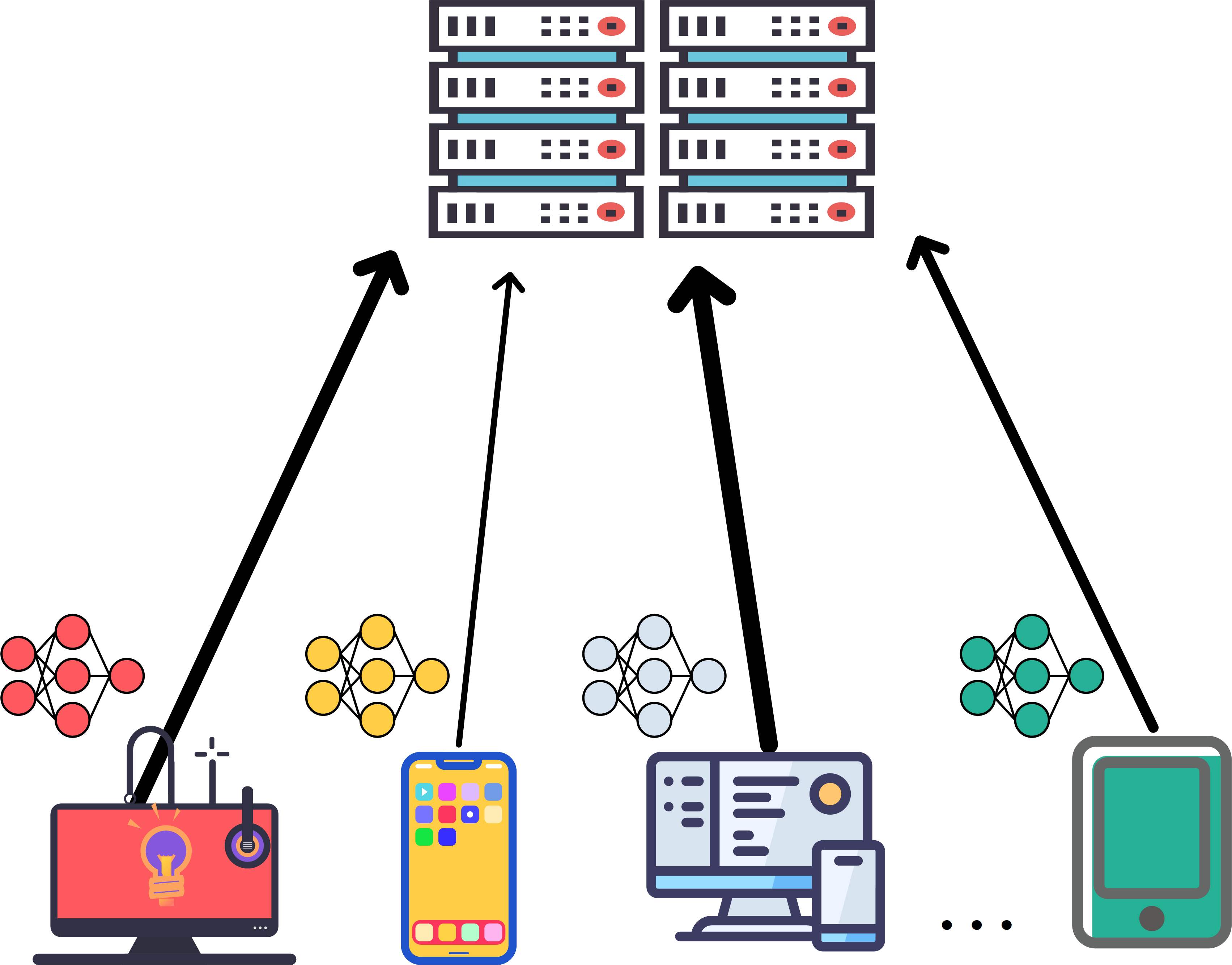
In fact, the models that clients upload have large data volumes, but the bandwidths among clients are different, and the bandwidth of each client is dynamic. The overview is illustrated in Fig. 1. Clients with poor bandwidth are waited for by the server for aggregate models, leading to low efficiency. Here, we consider the above bandwidth issues in federated learning scenario, propose a communication-efficient federated learning algorithm with adaptive compression under dynamic bandwidth, AdapComFL.
Different from traditional federated learning, client collects bandwidth data while training, predicts bandwidth of uplink communication, obtains data volume of uplink communication, subsequently determines the data volume of the upload model, and compresses model gradient by compression operator . The optimization objectives of AdapComFL are as follows:
| (2) |
where is local model weights for bandwidth prediction, is decompression operator, is the real time consumed for uplink communication, is real bandwidth, is the signal-to-noise ratio (SNR).
III-B Algorithm
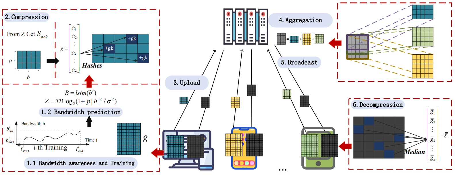
In this section, we propose the AdapComFL algorithm, which the workflow is illustrated in Fig. 2.
1) Bandwidth Awareness and Prediction: Each client is aware of the bandwidth during local model training, predicts bandwidth based on collected data, obtains the data volume of uplink communication, and determines the size of sketch model.
2) Compression: Each client adaptively compresses local model to sketch model.
3) Upload: Each client uploads the sketch model to server.
4) Aggregation: Server aggregates the sketch models which have different sizes.
5) Broadcast: Server sends aggregated sketch to each client.
6) Decompression: Each client decompresses sketch to recover the model.
Repeat steps 1-6 until the model converges. The detail of AdapComFL is shown in Algorithm 1.
In AdapComFL, to address the issues of communication bottleneck and improve accuracy in federated learning, there are two differences from traditional federated learning: bandwidth awareness and prediction; dynamic bandwidth-based local model compression.
Bandwidth awareness and prediction: In order to achieve communication efficiency in federated learning, each client first predicts the network bandwidth, computes the data volume of uplink communication, acquires the size of sketch model, and then, adaptively compresses the local model to sketch model.
In order to predict bandwidth, client first continuously collects bandwidth data via Iperf [33] while training, where is:
| (3) |
The bandwidth is predicted via a Long Short Term Memory (LSTM) recurrent neural network with one input layer, one output layer, and two hidden layers [34]. Suppose the sequence length of LSTM is , , the dataset is , during batch, the input data are , the label data is . When the training is completed, the output of LSTM is the predicted bandwidth .
Therefore, the data volume of uplink communication is obtained [35]:
| (4) |
Dynamic bandwidth-based local model compression in federated learning: To adaptively compress the local model gradient to the size of , we improve the sketch mechanism.
Generally, before client uploads the model gradient vector , the is compressed into sketch model with an matrix, each row corresponds to an independent hash function, which maps -dimensional to -dimensional space [30], , where
| (5) | |||
| (6) |
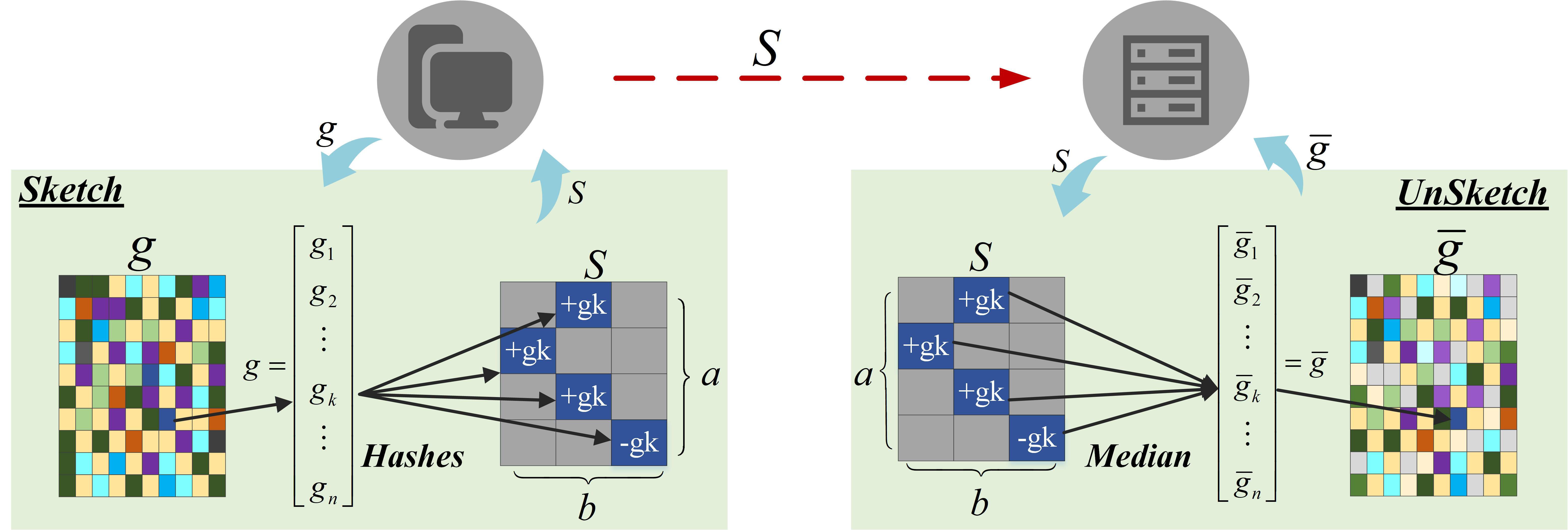
An overview of sketch mechanism is shown in Fig. 3, including compression and decompression. When client compresses the gradient vector , sketch model uses independent hash functions to map the to different columns within rows. Intuitively, for , the column position in the -th row is:
| (7) |
where . So the compression position of in sketch model is . Then the is accumulated into . Due to being much smaller than , there may be multiple gradients accumulated at the same position. For the position , the gradients accumulated at it are .
The traditional sketch mechanism fixes the size, clients with poor bandwidth experience longer times when uploading the sketch models. Additionally, multiple gradients accumulated at the same position result in poor accuracy when decompressing the sketch model to recover the global model.
To achieve adaptive bandwidth compression and improve accuracy in local model, unlike the general sketch mechanism, we fix columns and elastically adjust its rows, using the coefficient of variation to filter values that are mapped to the same position.
Suppose the sketch model of client is an matrix, where rows are obtained based on data volume and columns :
| (8) |
In compression operator , when complete the mappings, we process the values of each position in sketch. For the position , we process its values :
| (9) |
where
| (10) |
is the coefficient of variation of . Thus, client obtains compression model , and then uploads it to the server, where the data volume of upload is .
In aggregation operator , due to each client has different and , the is differ. As a result, the server can not aggregate sketch models. In this regard, we have two steps: first, size alignment of sketch models. For all sketch models from clients, the maximum number of rows is:
| (11) |
when , we fill the sketch model with zeros to rows, resulting in :
| (12) |
Second, aggregate all sketch models by calculate row-wise averages. To begin with, we obtain , which is the number of non-zero in each row of all sketch models. Then we aggregate the sketch models:
| (13) |
where is the aggregated sketch model.
Next, each client performs decompress operator after downloading the updated sketch model from the server:
| (14) |
| Dataset | Algorithm | Model | Learn Rate | Sketch | |
| Row | Column | ||||
| FEMNIST | FedAvg [1] | ResNet 56 | 0.001 | - | - |
| SketchFL [24] | ResNet 56 | 0.001 | 7 | 60000 | |
| AdapComFL | ResNet 56 | 0.001 | [3,10] | 60000 | |
| FashionMNIST | FedAvg [1] | ResNet 44 | 0.002 | - | - |
| SketchFL [24] | ResNet 44 | 0.002 | 7 | 50000 | |
| AdapComFL | ResNet 44 | 0.002 | [3,10] | 50000 | |
IV Evaluation
In this section, we present the setups and results of the experiment. The setups mainly have five parts: environments, datasets, models, parameters, and metrics. In the results, we evaluate the accuracy of bandwidth prediction, then show the performance of the AdapComFL algorithm, and compare it with other algorithms.
IV-A Setups
Environment: In order to simulate federated learning tasks, the experiments are implemented based on PyTorch [36] with an NVIDIA GeForce RTX 3090 GPU with 24 GB of memory.
Datasets: To evaluate the bandwidth prediction and the AdapComFL algorithm, we collect real bandwidth datasets and use two benchmark datasets.
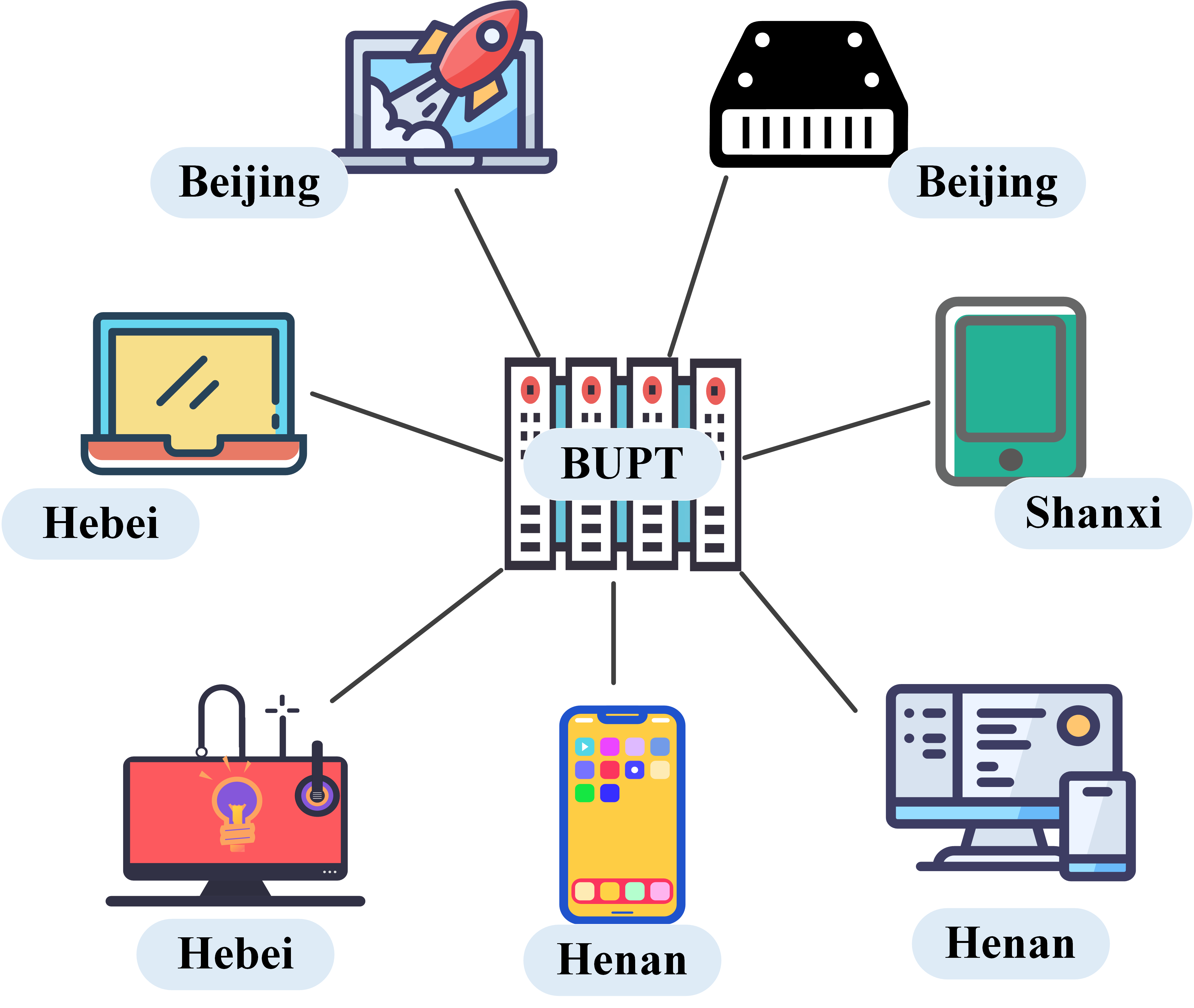
For bandwidth datasets, we build a network topology through Iperf [33] to collect bandwidth data which is show in Fig. 4. The collection equipments are different types of personal computers (PC), cell phones, and mini-PC, the locations are Beijing, Hebei, Henan, and Shanxi. We set up a server as the central node at the Beijing University of Posts and Telecommunications (BUPT). The 7 peripheral nodes have two serves: they function as probe nodes for collecting bandwidth data; they act as client nodes in federated learning. From July 1, 2022, to July 30, 2022, the network topology collects bandwidth continuously by seconds and every 24 hours generating one group. Thus, each probe node has a bandwidth dataset with 30 groups. Additionally, In upload process, the maximum time T for uplink communication in Eq. (4) is 0.5 s.
For benchmark datasets, we chose the public datasets FEMNIST [37] and FashionMNIST [38], which are processed to meet non-iid. FEMNIST is a handwritten digit recognition dataset containing 62 categories. FashionMNIST is an image classification dataset of fashion products for 10 categories.
Models and Parameters: This part describes neural network models and parameters in experiments. In the LSTM network used in bandwidth prediction, the input layer with 6 dimensions, the two hidden layers, each with 256 and 128 LSTM units respectively, and the size of the output layer is 1. The algorithms are experimented via Residual Network (ResNet) [39], the models and parameters are shown in Table I.
| Clients | |||||||
|---|---|---|---|---|---|---|---|
| #0 | #1 | #2 | #3 | #4 | #5 | #6 | |
| Raw BW | 12.72 | 4.81 | 2.59 | 1.73 | 0.42 | 1.78 | 0.93 |
| Pre BW | 12.82 | 4.76 | 2.51 | 1.77 | 0.41 | 1.77 | 0.94 |
Metrics: In order to evaluate accuracy and communication efficiency of AdapComFL algorithm, some metrics are selected.
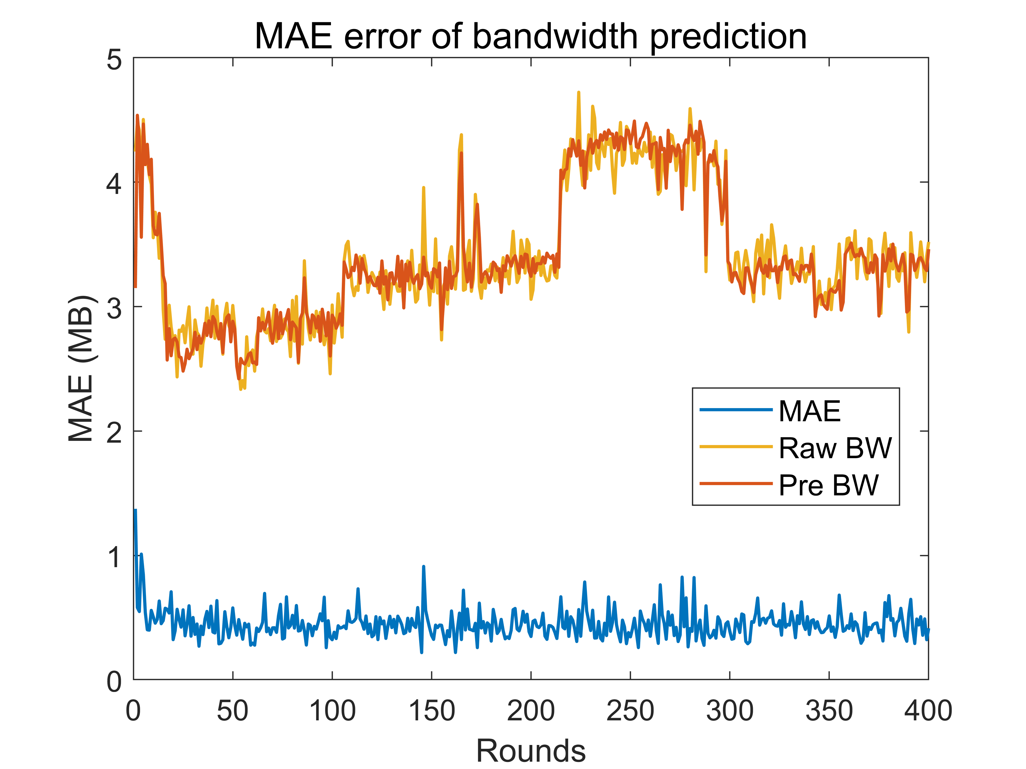
In accuracy, we consider the bandwidth prediction and the algorithm. For bandwidth prediction, we evaluate the accuracy by Mean Absolute Error (MAE). The formula of is given by
| (15) |
where is the number of . The accuracy of prediction increases as decreases. The accuracy of alogorithm is:
| (16) |
where is the number of correctly classified samples.
In communication efficiency, we consider the compression ratio . where is the data volume of uplink communication by clients in the FedAvg algorithm, which is a constant, and reflects the compression degree of the model, which as decreases, the compression level increases, the time and the data volume of uplink communication are reduce. The compression ratio
IV-B Results
In this section, we compare the AdapComFL algorithm with other algorithms for accuracy and communication efficiency.
Accuracy: We show the accuracy of bandwidth prediction and algorithms.
The accuracy of bandwidth prediction can be shown in Fig. 5. It illustrates the accuracy of bandwidth prediction through overall error, where Raw BW (MB) is the average of bandwidth real data, Pre BW (MB) is the average of bandwidth prediction data. From Fig. 5, the Pre BW fits the Raw BW by LSTM prediction and the error is around 0.5 MB, which implies AdapComFL has favorable accuracy in bandwidth prediction. Table II shows each client’s average value of Raw BW and Pre BW. The similarity of the data further confirms the validity of the bandwidth prediction.
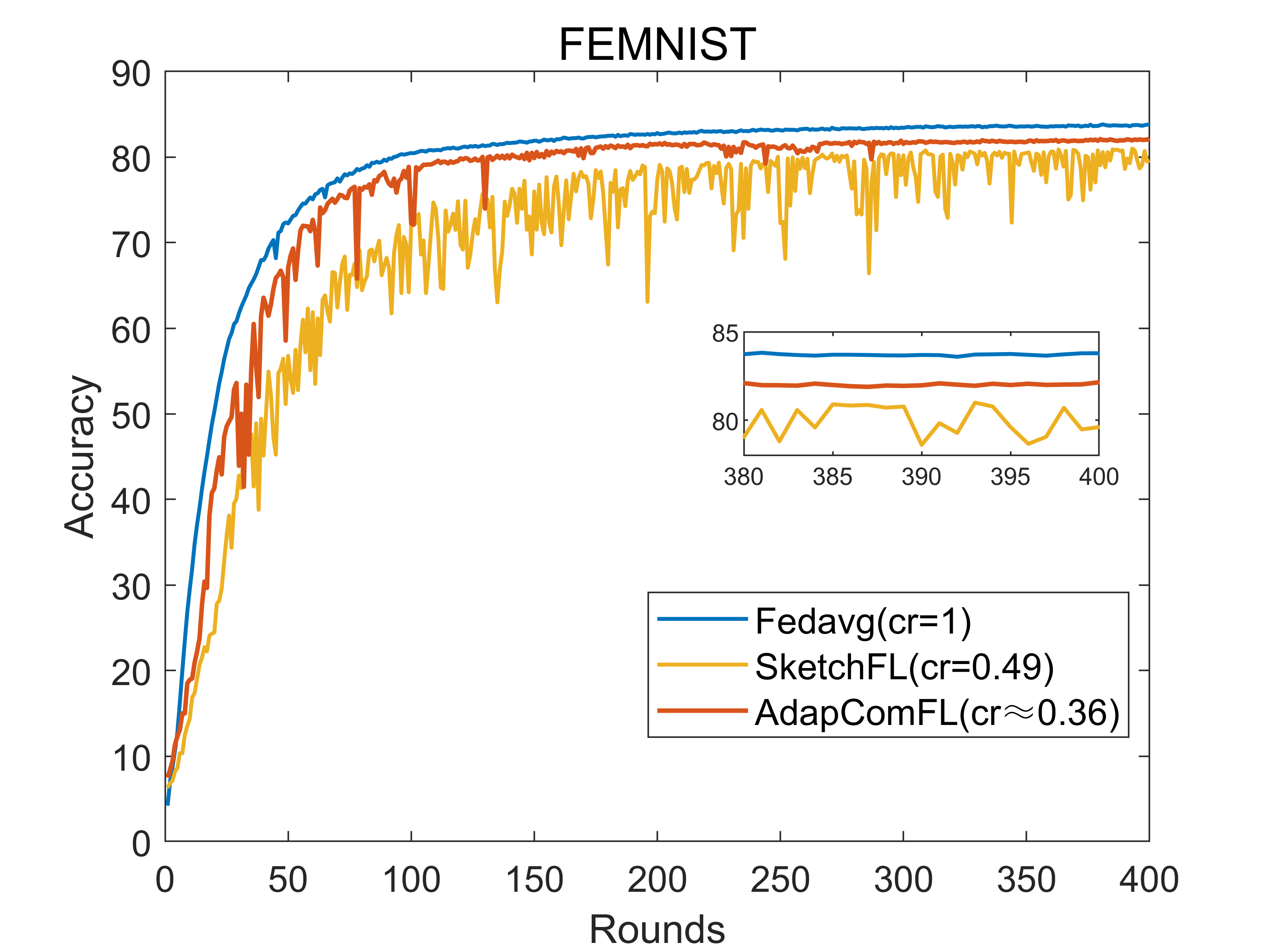
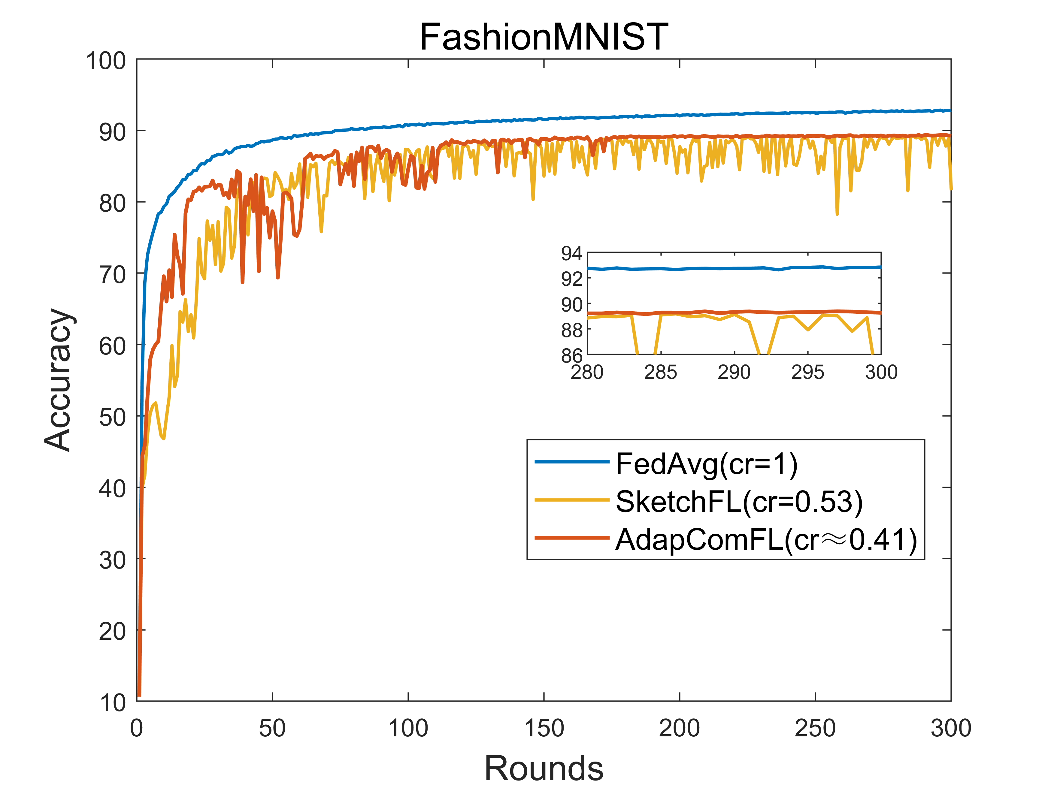
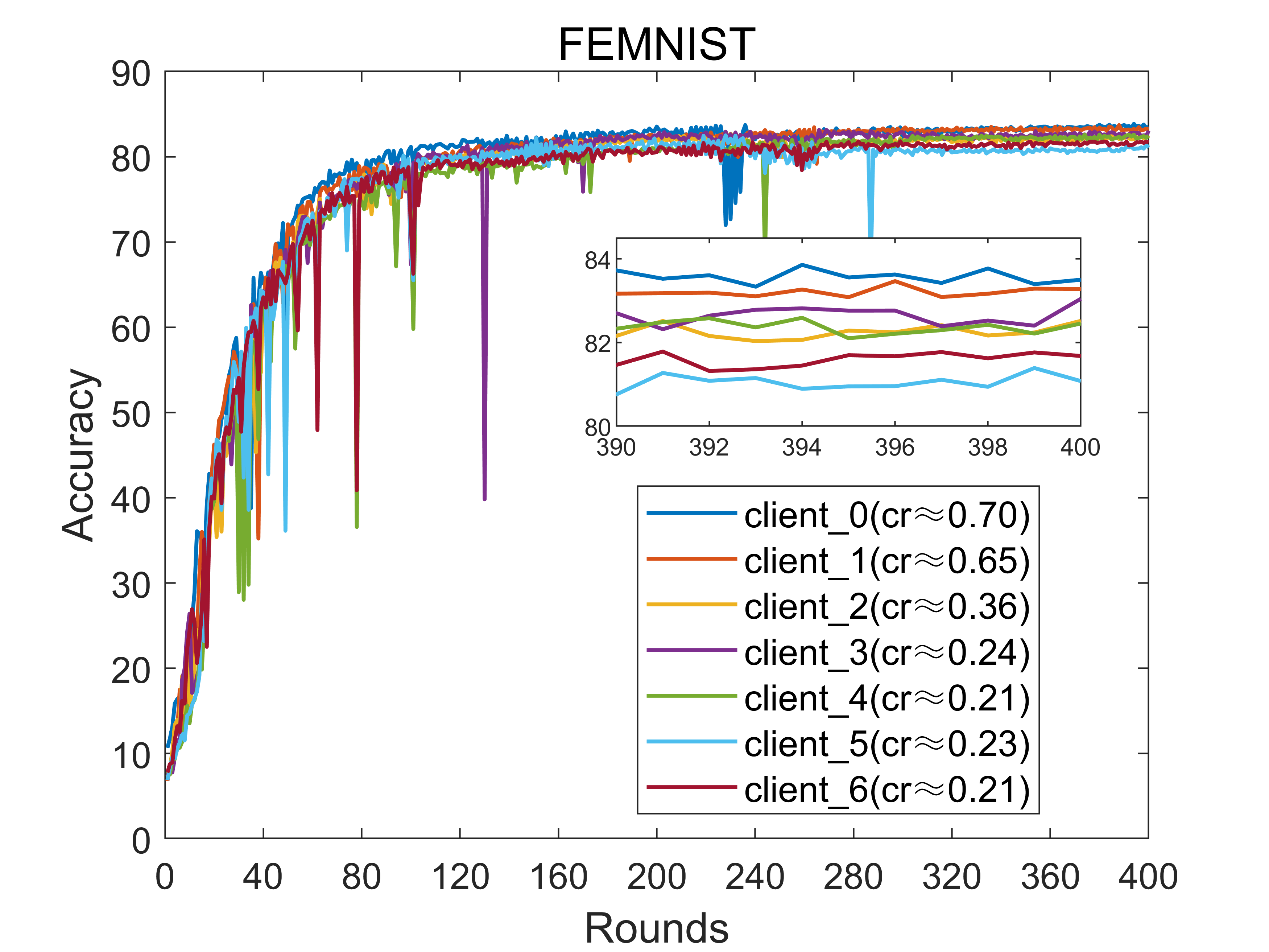
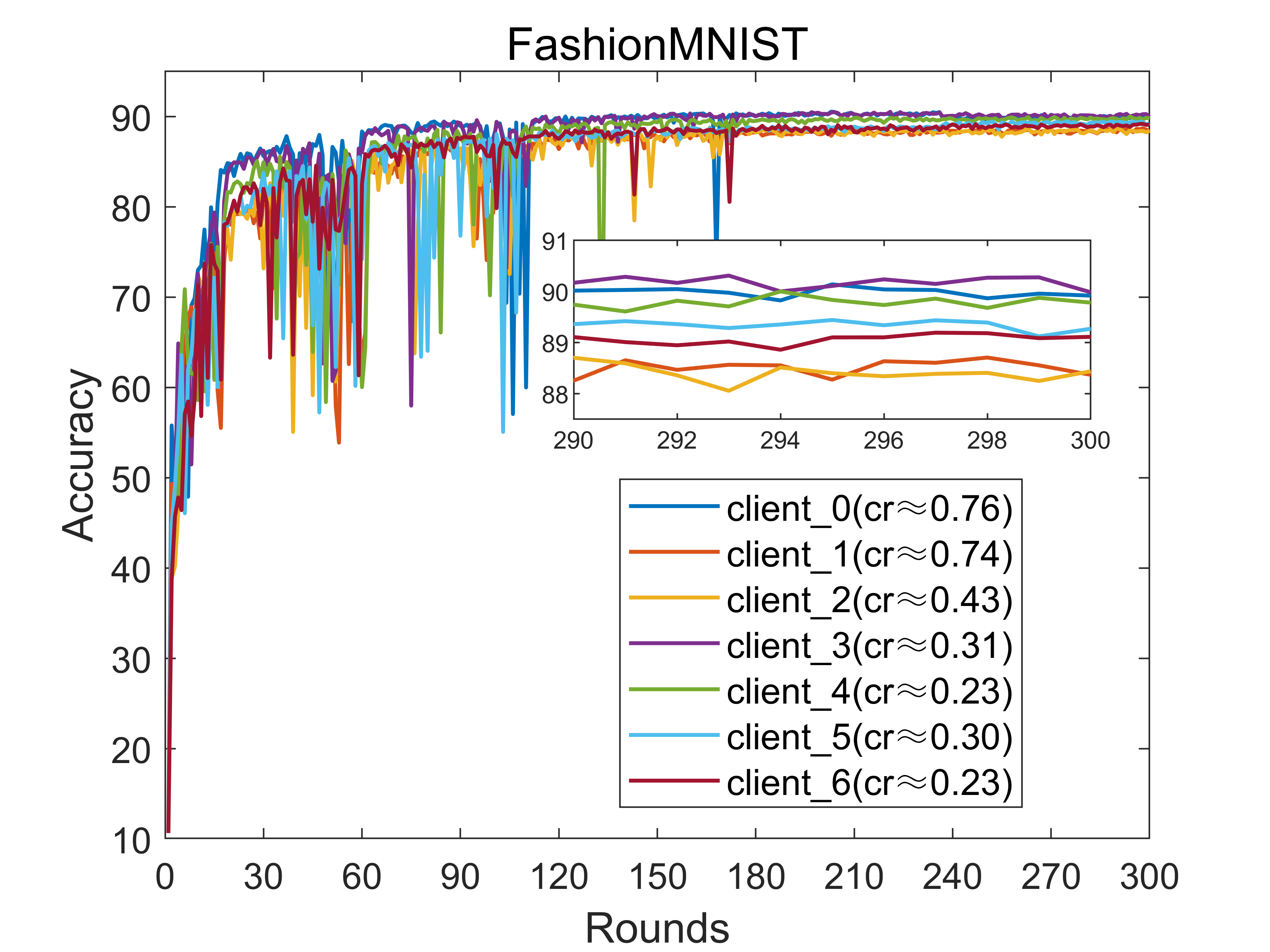
We then present the accuracy of AdapComFL on FEMNIST and FashionMNIST, comparing it with FedAvg and SketchFL, as shown in Fig. 6LABEL:sub@femnist_acc and 7LABEL:sub@fashion_acc. In these figures, the AdapComFL algorithm at a lower compression ratio outperforms slightly inferior to FedAvg in accuracy but has higher accuracy and more stable results than SketchFL. The compression method of the sketch is lossy, but we maintain favorable accuracy by improving the sketch mechanism. The experimental results imply that the improvement is effectual. In particular, it is even more evident in the FEMNIST dataset. The above accuracy focus on the aggregation models. For each client in our AdapComFL, the accuracy is as shown in Fig. 9LABEL:sub@femnist_client_acc, 10LABEL:sub@fashion_client_acc. Despite variations in compression ratios, the clients present high-accuracy.
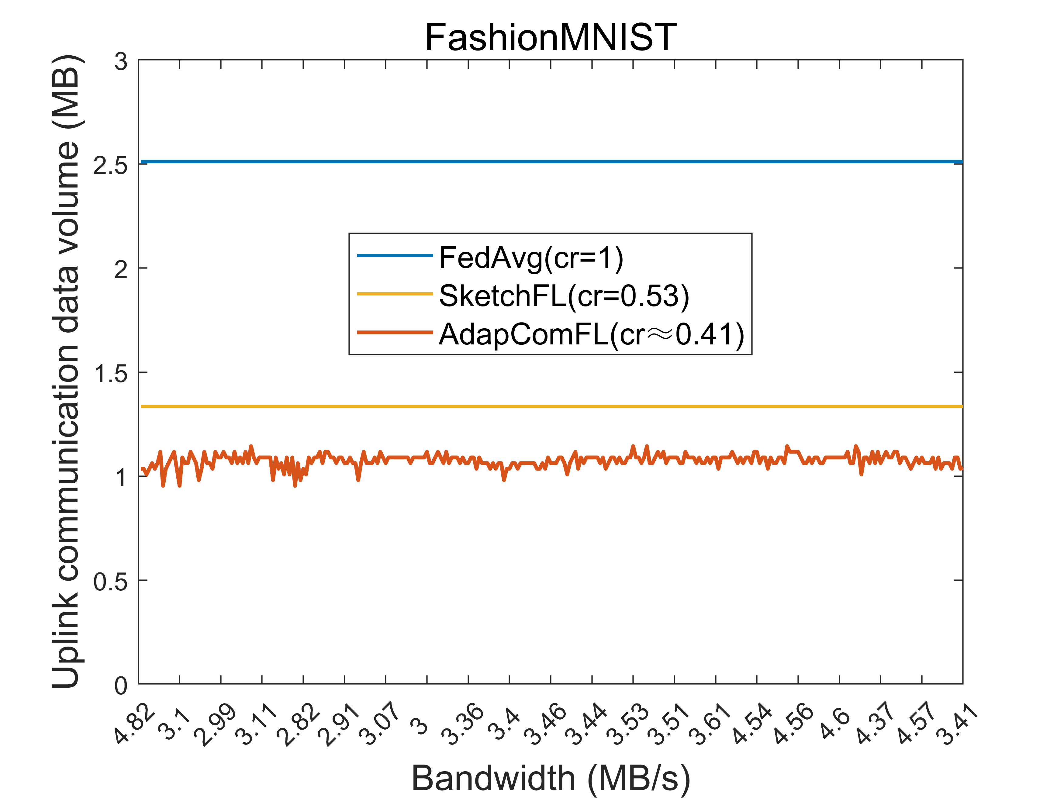
Communication efficiency: We compared the communication efficiency of AdapComFL algorithm with other algorithms from communication time, communication data volume, and compression ratio.
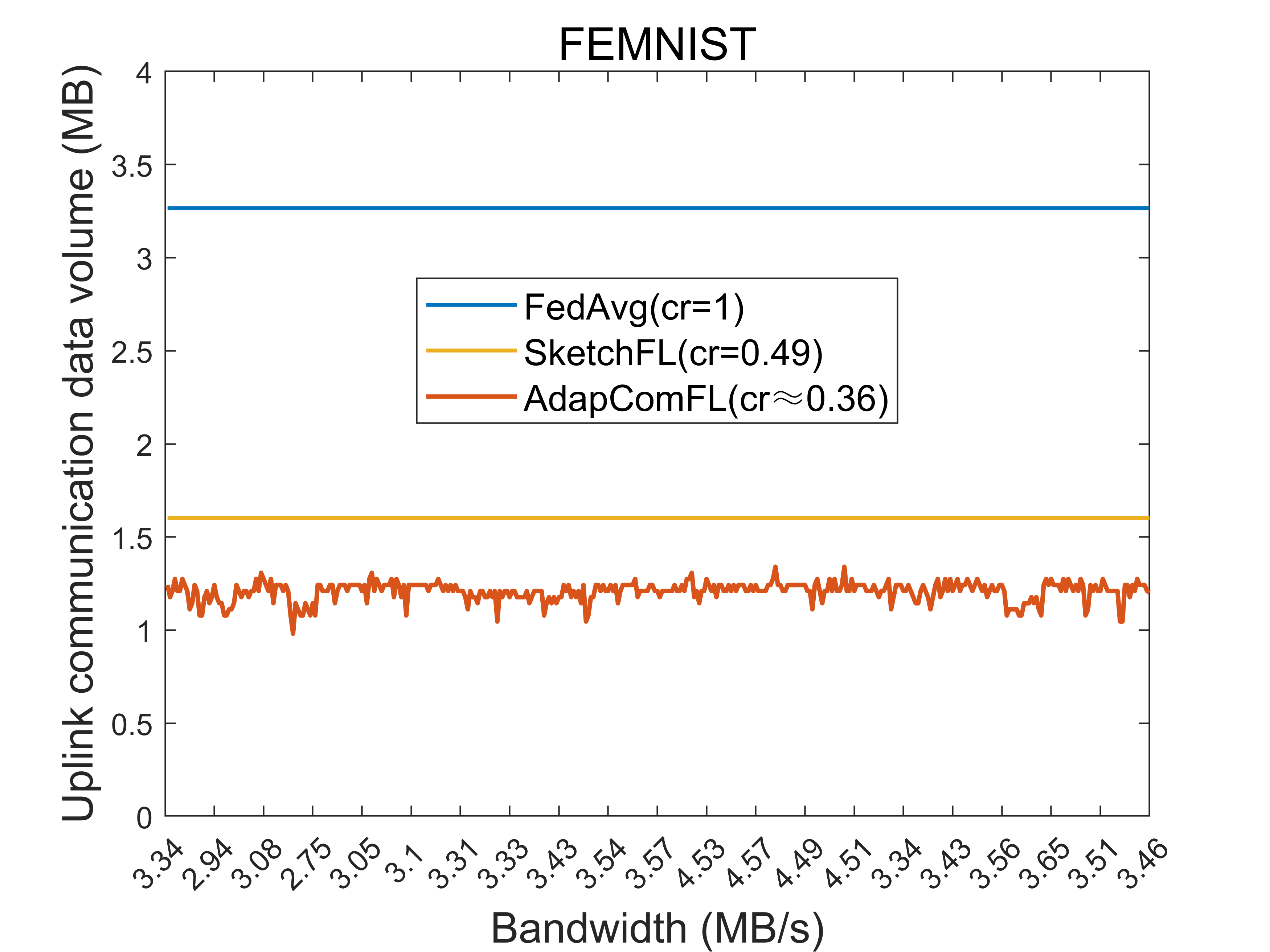
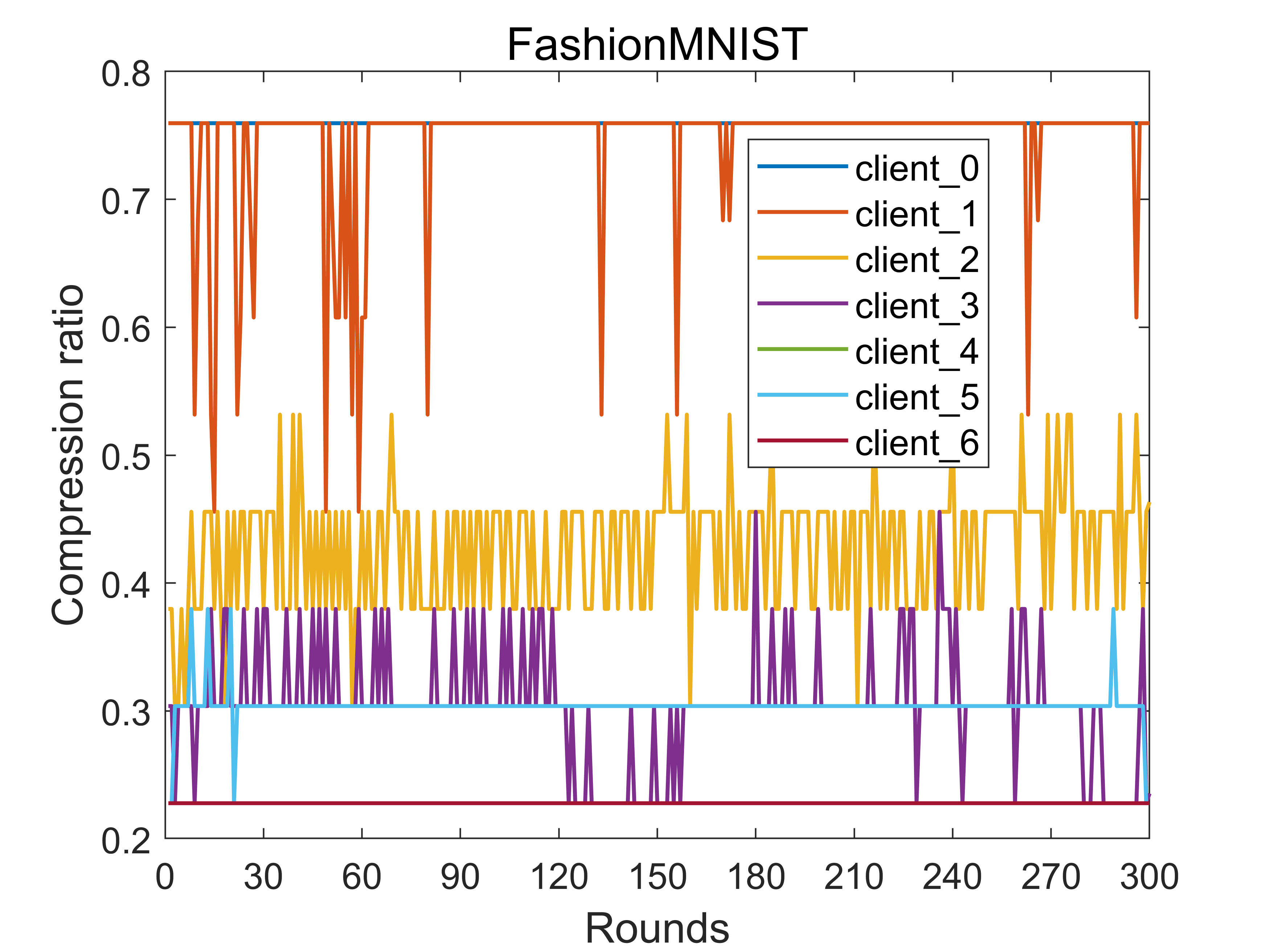
The communication data volume is shown in Fig. 6LABEL:sub@femnist_cost and 7LABEL:sub@fashion_cost. It can be observed that the FedAvg algorithm presents high and constant data volume due to it uploading uncompressed models. The SketchFL algorithm has constant data volume due to the fixed compression ratio. In contrast, our proposed AdapComFL fluctuates data volume due to the adaptive compression model based on bandwidth conditions.
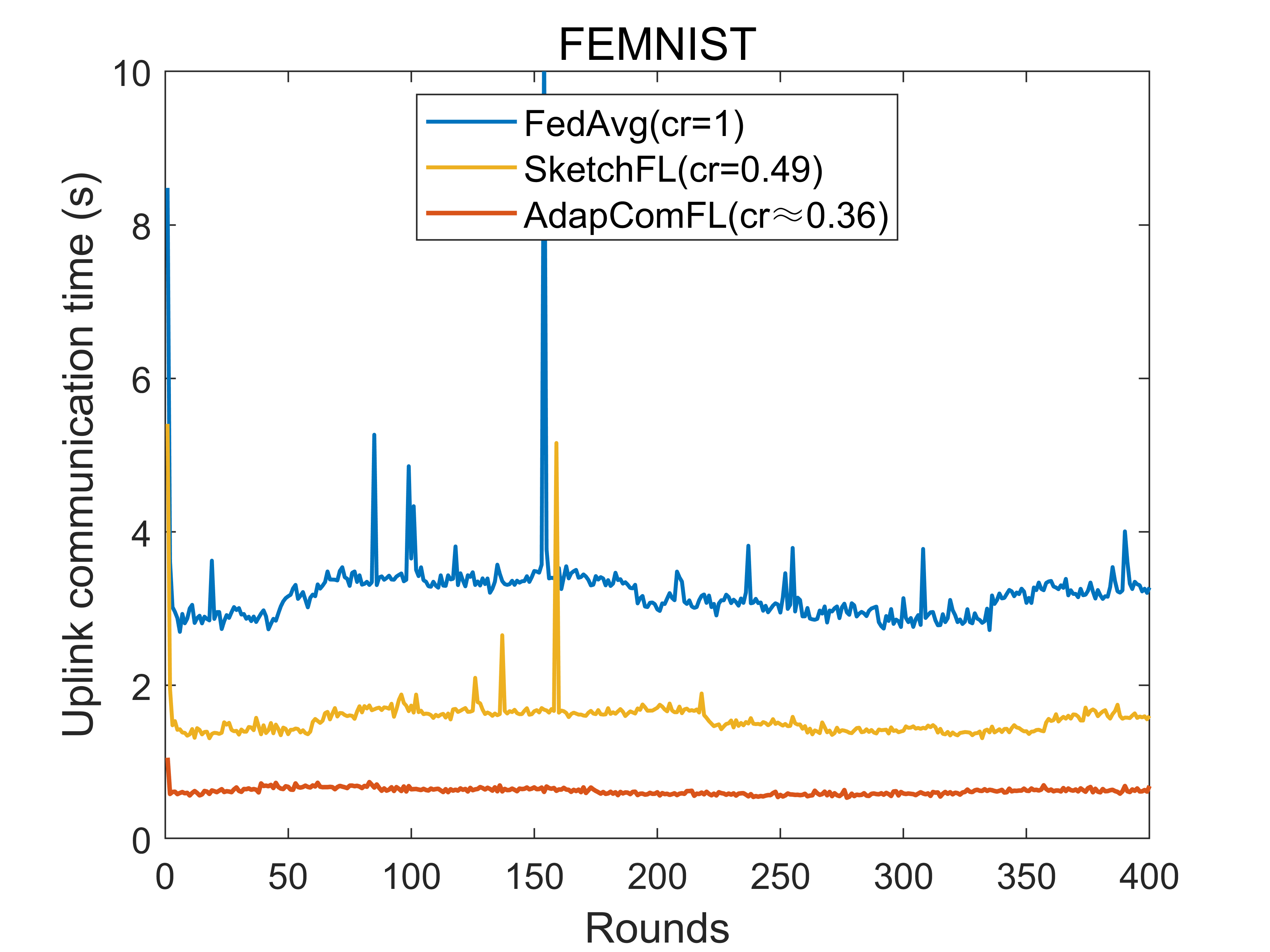
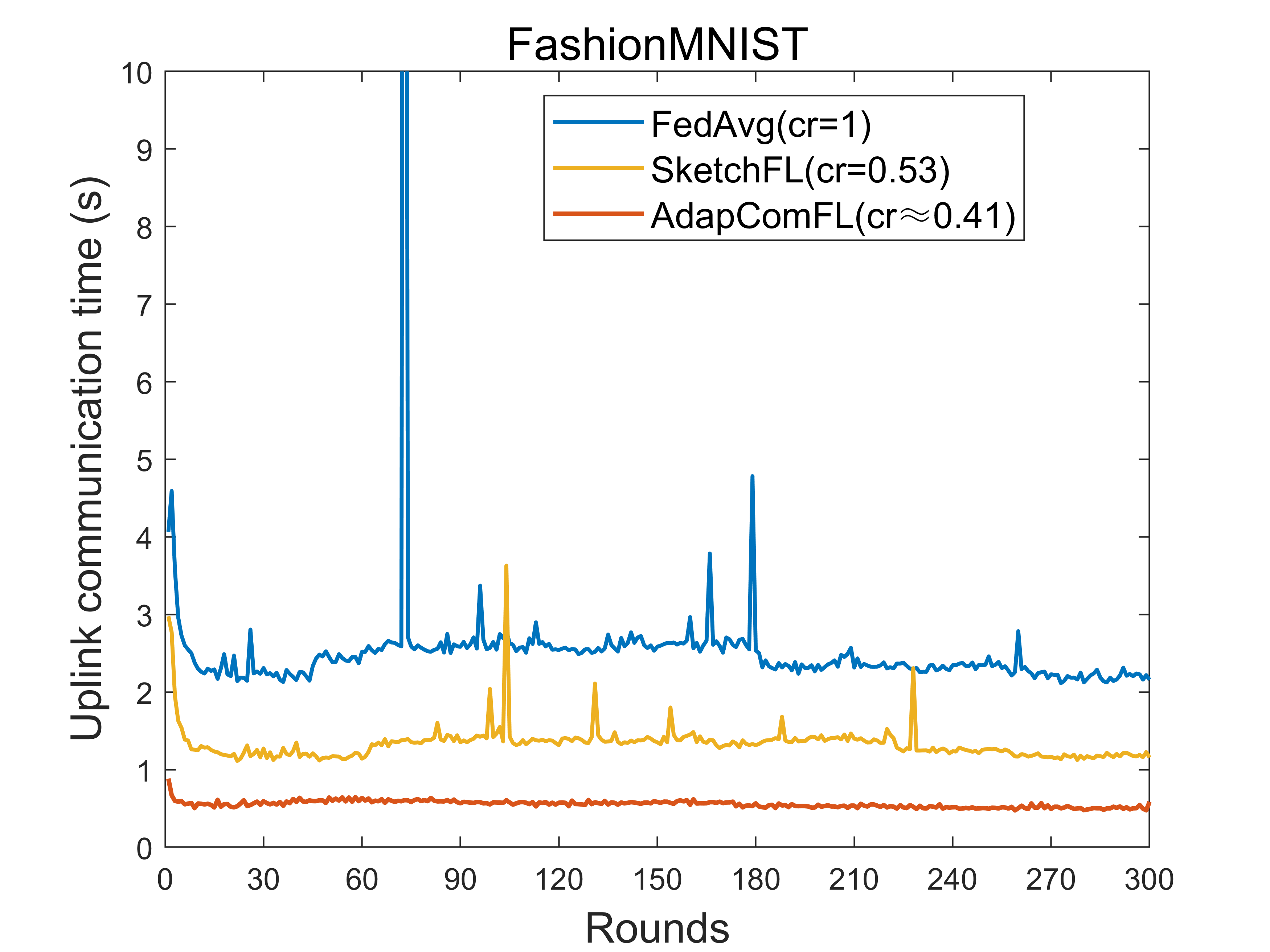
We then present the communication time in Fig. 6LABEL:sub@femnist_time and 7LABEL:sub@fashion_time. FedAvg and SketchFL take longer times to upload, but AdapComFL completes the upload around 0.5 s, which meets the maximum time we have set. It is evident that we achieve communication efficiency. Considering some clients with poor bandwidth conditions, the maximum compression may still exceed the maximum time.
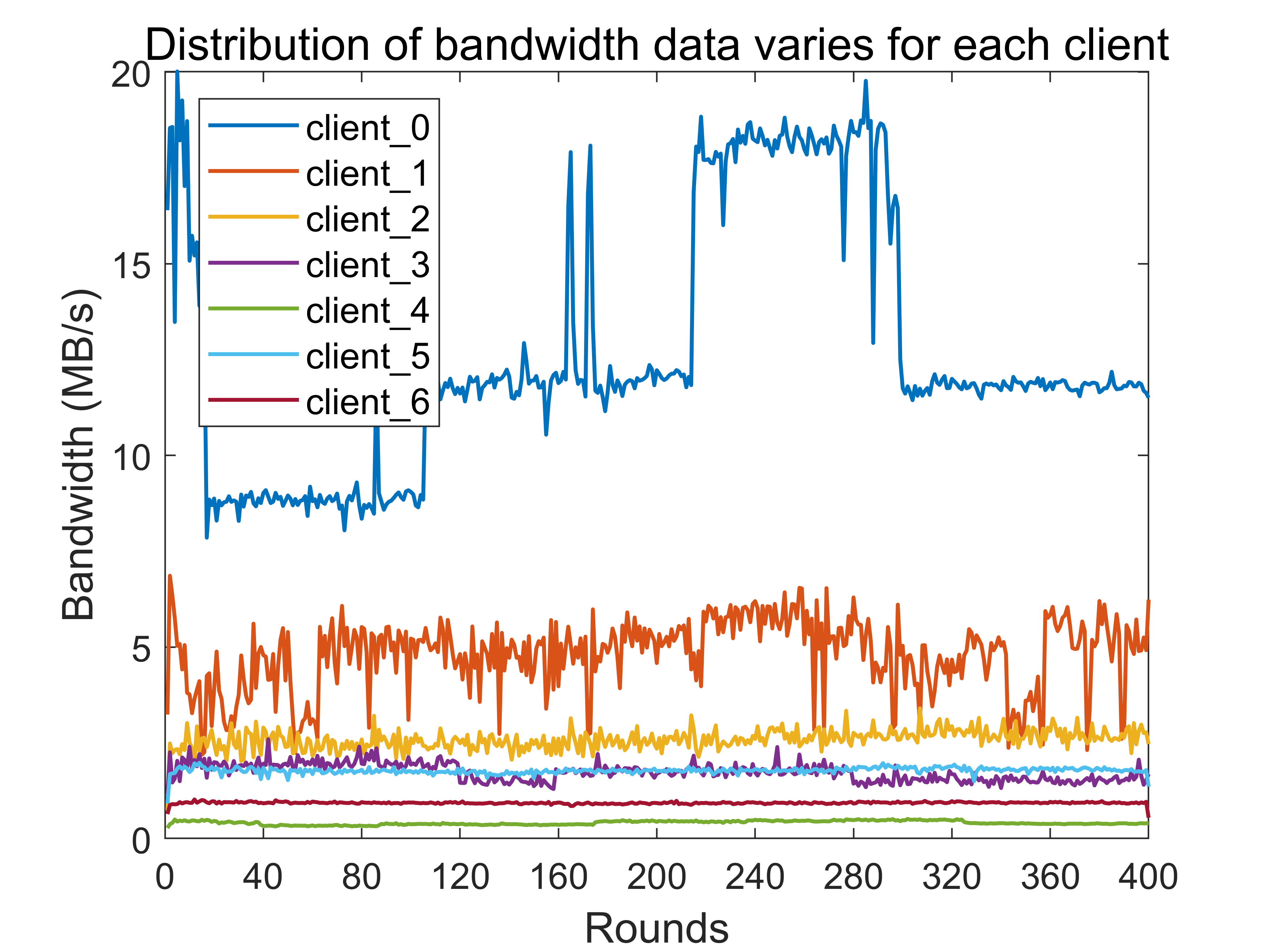
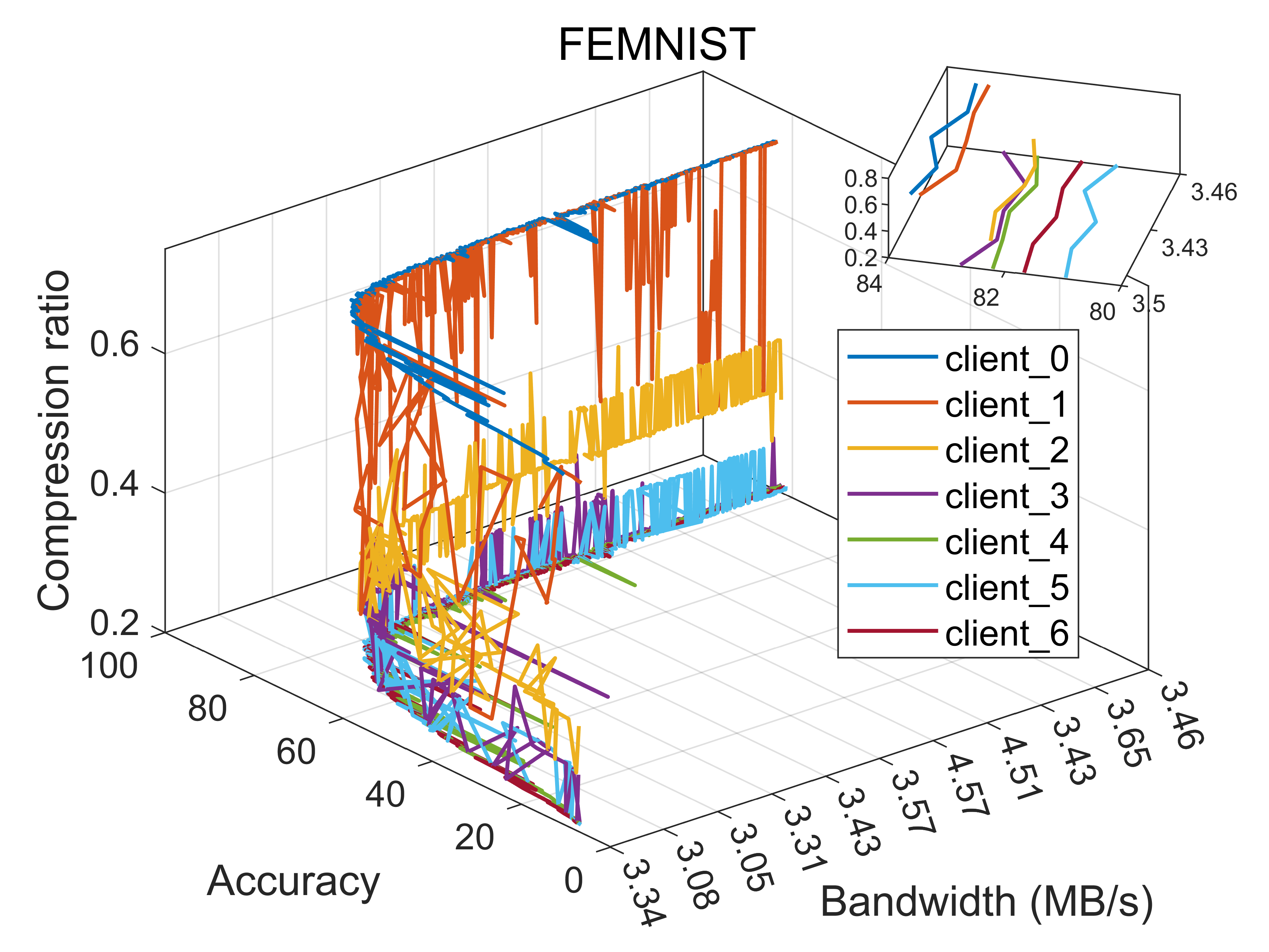
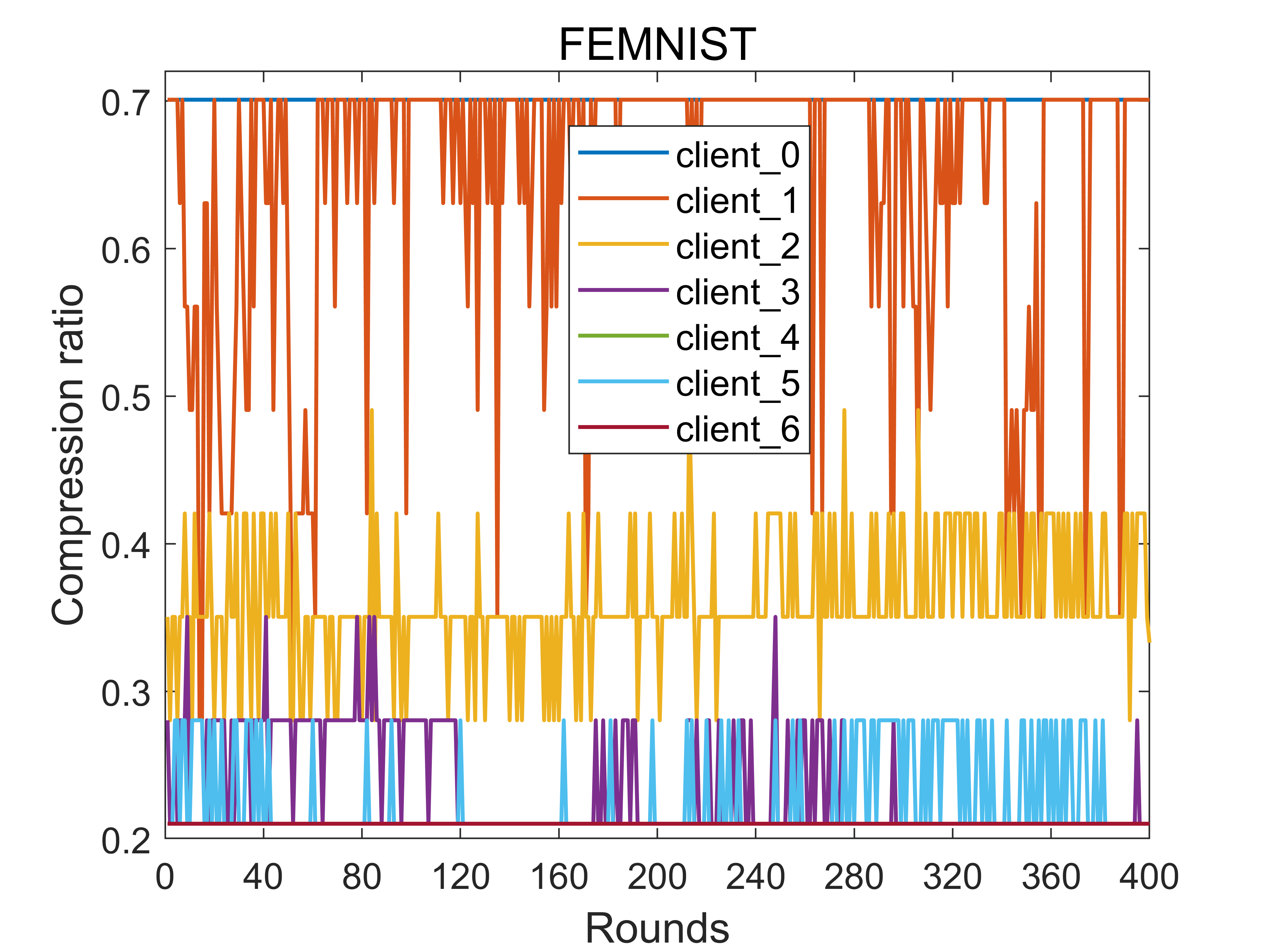
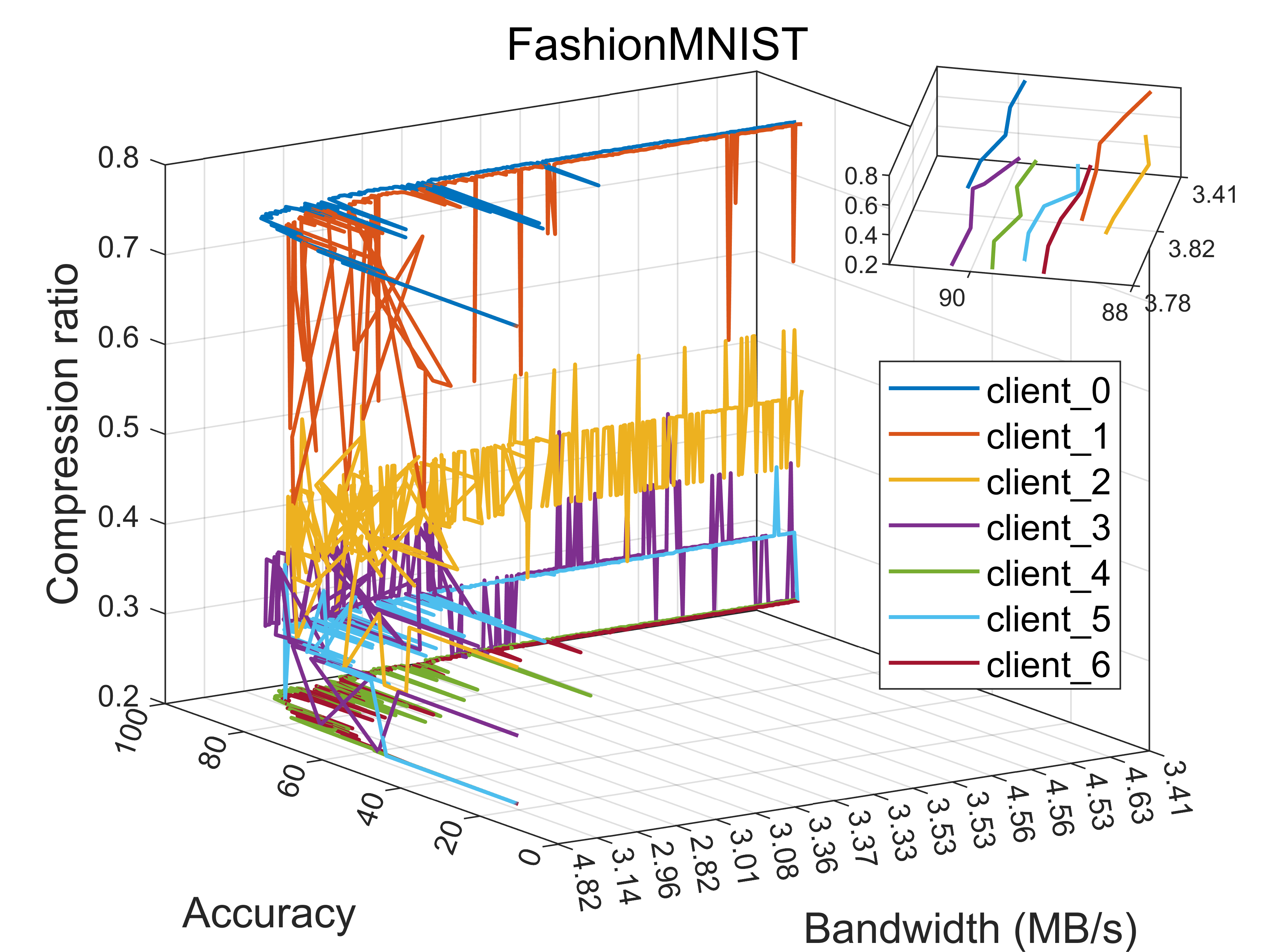
Actually, the above results are the average outcomes for clients and the fluctuation is not large enough. We show the results of each client from the network bandwidth and performance in our AdapComFL. In network bandwidth, the distribution for each client is shown in Fig. 8. The curves of the clients show significant differences because they have various bandwidth conditions. We then discuss the results of bandwidth, accuracy, and compression ratio in Fig. 9LABEL:sub@femnist_user_3d and 10LABEL:sub@fashion_user_3d on FEMNIST and FashionMNIST. In order to provide a more intuitive understanding of the accuracy and compression ratio for each client, we present Fig. 9LABEL:sub@femnist_client_acc, 9LABEL:sub@femnist_client_ratio for FEMNIST, and 10LABEL:sub@fashion_client_acc, 10LABEL:sub@fashion_client_ratio for FashionMNIST. Before each round of upload, clients aware of and predict the network bandwidth, then compress the model adaptively. The clients with poor bandwidth conditions achieve communication efficiency by heavily compressing the local model, while maintaining high accuracy. The clients with strong bandwidth conditions utilize bandwidth resources effectively by lightly compressing the model, which obtains high accuracy.
V Conclusions
In this article, we address the communication efficiency problem with federated learning. To overcome the bandwidth issues in communication efficiency, we propose AdapComFL algorithm, in which each client predicts its bandwidth and adaptively compresses the model gradient with the sketch method. In addition, we improve the sketch-based compression mechanism to alleviate the error. We perform experiments through real bandwidth datasets and benchmark datasets, with the bandwidth datasets collected from the network topology we build. The experiments compare the AdapComFL algorithm with the FedAvg and SketchFL algorithms in accuracy and communication efficiency. The results demonstrate that AdapComFL predicts the bandwidth with low error, and achieves communication efficiency of federated learning. Moreover, the improved sketch mechanism not only boosts the accuracy of AdapComFL but also leads to more stable results.
References
- [1] B. McMahan, E. Moore, D. Ramage, S. Hampson, and B. A. y Arcas, “Communication-efficient learning of deep networks from decentralized data,” in Proc. Artif. Intell. Stat. (AISTATS). Fort Lauderdale, Florida, USA: PMLR, Apr. 2017, pp. 1273–1282.
- [2] K. Zhang, J. Ni, K. Yang, X. Liang, J. Ren, and X. S. Shen, “Security and privacy in smart city applications: Challenges and solutions,” IEEE Commun. Mag., vol. 55, no. 1, pp. 122–129, Jan. 2017.
- [3] R. Petrolo, V. Loscri, and N. Mitton, “Towards a smart city based on cloud of things, a survey on the smart city vision and paradigms,” Trans. Emerg. Telecommun. Technol., vol. 28, no. 1, p. e2931, Mar. 2017.
- [4] P. Voigt and A. Von dem Bussche, “The eu general data protection regulation (gdpr),” Springer International Publishing, Aug. 2017.
- [5] P. Kairouz, H. B. McMahan, B. Avent, A. Bellet, M. Bennis, A. N. Bhagoji, K. Bonawitz, Z. Charles, G. Cormode, R. Cummings et al., “Advances and open problems in federated learning,” Found. Trends. Mach. Le., vol. 14, no. 1–2, pp. 1–210, Jun. 2021.
- [6] Q. Yang, Y. Liu, T. Chen, and Y. Tong, “Federated machine learning: Concept and applications,” ACM Trans. Intell. Syst. Technol., vol. 10, no. 2, pp. 1–19, Jan. 2019.
- [7] T. Li, A. K. Sahu, A. Talwalkar, and V. Smith, “Federated learning: Challenges, methods, and future directions,” IEEE Signal Proc. Mag., vol. 37, no. 3, pp. 50–60, May 2020.
- [8] J. Konečnỳ, “Stochastic, distributed and federated optimization for machine learning,” arXiv preprint arXiv:1707.01155, Jul. 2017.
- [9] T. Li, A. K. Sahu, M. Zaheer, M. Sanjabi, A. Talwalkar, and V. Smith, “Federated optimization in heterogeneous networks,” Proc. Mach. Learn. Syst. (MLSys), vol. 2, pp. 429–450, Mar. 2020.
- [10] S. Ji, W. Jiang, A. Walid, and X. Li, “Dynamic sampling and selective masking for communication-efficient federated learning,” IEEE Intell. Syst., vol. 37, no. 2, pp. 27–34, Sep. 2021.
- [11] Y. Lin, S. Han, H. Mao, Y. Wang, and W. J. Dally, “Deep gradient compression: Reducing the communication bandwidth for distributed training,” arXiv preprint arXiv:1712.01887, Dec. 2017.
- [12] J. Konečnỳ, H. B. McMahan, F. X. Yu, P. Richtárik, A. T. Suresh, and D. Bacon, “Federated learning: Strategies for improving communication efficiency,” arXiv preprint arXiv:1610.05492, Oct. 2016.
- [13] F. Sattler, S. Wiedemann, K.-R. Müller, and W. Samek, “Robust and communication-efficient federated learning from non-iid data,” IEEE Trans. Neural Netw. Learn. Syst., vol. 31, no. 9, pp. 3400–3413, Nov. 2019.
- [14] C. Li, G. Li, and P. K. Varshney, “Communication-efficient federated learning based on compressed sensing,” IEEE Internet Things J., vol. 8, no. 20, pp. 15 531–15 541, 2021.
- [15] Y. He, M. Zenk, and M. Fritz, “Cossgd: Nonlinear quantization for communication-efficient federated learning,” arXiv preprint arXiv:2012.08241, Dec. 2020.
- [16] D. Alistarh, D. Grubic, J. Li, R. Tomioka, and M. Vojnovic, “Qsgd: Communication-efficient sgd via gradient quantization and encoding,” Proc. Adv. Neural Inf. Process. Syst. (NeurIPS), vol. 30, May 2017.
- [17] J. Xu, W. Du, Y. Jin, W. He, and R. Cheng, “Ternary compression for communication-efficient federated learning,” IEEE Trans. Neural Netw. Learn. Syst., Dec. 2020.
- [18] W.-T. Chang and R. Tandon, “Communication efficient federated learning over multiple access channels,” arXiv preprint arXiv:2001.08737, Jan. 2020.
- [19] D. Jhunjhunwala, A. Gadhikar, G. Joshi, and Y. C. Eldar, “Adaptive quantization of model updates for communication-efficient federated learning,” in Proc. IEEE Int. Conf. Acoust. Speech Signal Process. (ICASSP). Toronto, Canada: IEEE, May 2021, pp. 3110–3114.
- [20] A. Reisizadeh, A. Mokhtari, H. Hassani, A. Jadbabaie, and R. Pedarsani, “Fedpaq: A communication-efficient federated learning method with periodic averaging and quantization,” in Proc. Int. Conf. Artif. Intell. Stat. (ICAIS). PMLR, 2020, pp. 2021–2031.
- [21] M. M. Amiri, D. Gunduz, S. R. Kulkarni, and H. V. Poor, “Federated learning with quantized global model updates,” arXiv preprint arXiv:2006.10672, 2020.
- [22] H. Zhang, J. Liu, J. Jia, Y. Zhou, H. Dai, and D. Dou, “Fedduap: Federated learning with dynamic update and adaptive pruning using shared data on the server,” arXiv preprint arXiv:2204.11536, Apr. 2022.
- [23] Y. Jiang, S. Wang, V. Valls, B. J. Ko, W.-H. Lee, K. K. Leung, and L. Tassiulas, “Model pruning enables efficient federated learning on edge devices,” IEEE Trans. Neural Netw. Learn. Syst., Apr. 2022.
- [24] Z. Liu, T. Li, V. Smith, and V. Sekar, “Enhancing the privacy of federated learning with sketching,” arXiv preprint arXiv:1911.01812, Nov. 2019.
- [25] H. Abdi, “Coefficient of variation,” Encycl. Res. Des., vol. 1, no. 5, Aug. 2010.
- [26] P. Han, S. Wang, and K. K. Leung, “Adaptive gradient sparsification for efficient federated learning: An online learning approach,” in Proc. IEEE 40th Int. Conf. Distrib. Comput. Syst. (ICDCS). Tamilnadu, India: IEEE, Nov. 2020, pp. 300–310.
- [27] E. Ozfatura, K. Ozfatura, and D. Gündüz, “Time-correlated sparsification for communication-efficient federated learning,” in 2021 IEEE Int. Symposium on Info. Theory (ISIT). Melbourne, Australia: IEEE, Jul. 2021, pp. 461–466.
- [28] E. Jeong, S. Oh, H. Kim, J. Park, M. Bennis, and S.-L. Kim, “Communication-efficient on-device machine learning: Federated distillation and augmentation under non-iid private data,” arXiv preprint arXiv:1811.11479, Nov. 2018.
- [29] F. Sattler, A. Marban, R. Rischke, and W. Samek, “Communication-efficient federated distillation,” arXiv preprint arXiv:2012.00632, Dec. 2020.
- [30] T. Li, Z. Liu, V. Sekar, and V. Smith, “Privacy for free: Communication-efficient learning with differential privacy using sketches,” arXiv preprint arXiv:1911.00972, Nov. 2019.
- [31] M. Charikar, K. Chen, and M. Farach-Colton, “Finding frequent items in data streams,” in Proc. Int. Colloq. Automata, Lang., Program. (ICALP). Springer, Jan. 2002, pp. 693–703.
- [32] D. Rothchild, A. Panda, E. Ullah, N. Ivkin, I. Stoica, V. Braverman, J. Gonzalez, and R. Arora, “Fetchsgd: Communication-efficient federated learning with sketching,” in Int. Conf. on Machine Learning (ICML). Online: PMLR, Jul. 2020, pp. 8253–8265.
- [33] A. Tirumala, “Iperf: The tcp/udp bandwidth measurement tool,” http://dast. nlanr. net/Projects/Iperf/, May 2005.
- [34] L. Mei, R. Hu, H. Cao, Y. Liu, Z. Han, F. Li, and J. Li, “Realtime mobile bandwidth prediction using lstm neural network and bayesian fusion,” Comput. Netw., vol. 182, p. 107515, 2020.
- [35] J. Xu and H. Wang, “Client selection and bandwidth allocation in wireless federated learning networks: A long-term perspective,” IEEE Trans. Wirel. Commun., vol. 20, no. 2, pp. 1188–1200, 2020.
- [36] A. Paszke, S. Gross, F. Massa, A. Lerer, J. Bradbury, G. Chanan, T. Killeen, Z. Lin, N. Gimelshein, L. Antiga et al., “Pytorch: An imperative style, high-performance deep learning library,” Proc. Advances in Neural Inf. Process. Syst. (NIPS), vol. 32, Dec. 2019.
- [37] S. Caldas, S. M. K. Duddu, P. Wu, T. Li, J. Konečnỳ, H. B. McMahan, V. Smith, and A. Talwalkar, “Leaf: A benchmark for federated settings,” arXiv preprint arXiv:1812.01097, Dec. 2018.
- [38] H. Xiao, K. Rasul, and R. Vollgraf, “Fashion-mnist: a novel image dataset for benchmarking machine learning algorithms,” arXiv preprint arXiv:1708.07747, Aug. 2017.
- [39] K. He, X. Zhang, S. Ren, and J. Sun, “Deep residual learning for image recognition,” in Proc. IEEE Conf. Comp. Vis. Patt. Recogn. (CVPR), Las Vegas, NV, USA, Jun. 2016, pp. 770–778.