A First-Engineering Principles Model for Dynamical Simulation of a Calciner in Cement Production

Abstract

We present an index-1 differential-algebraic equation (DAE) model for dynamic simulation of a calciner in the pyro-section of a cement plant. The model is based on first engineering principles and integrates reactor geometry, thermo-physical properties, transport phenomena, stoichiometry and kinetics, mass and energy balances, and algebraic volume and internal energy equations in a systematic manner. The model can be used for dynamic simulation of the calciner. We also provide simulation results that are qualitatively correct. The calciner model is part of an overall model for dynamical simulation of the pyro-section in a cement plant. This model can be used in design of control and optimization systems to improve the energy efficiency and CO2 emission from cement plants.

1 Introduction

The production of cement clinker is the main source of CO2 emissions in cement manufacturing. Cement manufacturing is responsible for 8% of the global CO2 emissions and about 25% of all industrial CO2 emissions (Lehne and Preston, 2018). Along with process modifications for carbon capture and storage (CCS), digitalization, control, and optimization are important tools in the transition to zero CO2-emission cement plants. Development of such digitalization, control and optimization tools require dynamic simulation and digital twins for the cement plant, and the pyro-section in particular. Mathematical models for dynamic simulation of the pyro-section in cement plants are not available. Fig. 1 illustrates the pyro-section of a cement plant. The pyro-section consists of pre-heating cyclones, a calciner, a rotary kiln, and a cooler. In this paper, we provide a mathematical model for dynamic simulation of the calciner. A related paper provides a mathematical model for dynamic simulation of the rotary kiln (Svensen et al., 2024), while papers for the pre-heating cyclones and the cooler are being prepared. Accordingly, the contribution of this paper is a dynamic simulation model for a subunit in the pyro-processing section of a cement plant, namely the calciner. This model is relevant for traditional cement plants as well as modern cement plants designed for carbon capture (oxy-combustion with carbon capture or post carbon capture) and useful for design of control and optimization systems for such plants.

Figure 1: The pyro-section for production of cement clinker in a cement plant consists of preheating cyclones (P), a calciner (Ca), a rotary kiln (K), and a cooler (Co).

Mujumdar et al. (2007) modeled a cyclone-based calciner using a quasi steady state approximation for the coal particles and a dynamic description for the raw meal and gases. Kahawalage et al. (2017) used a CFD approach to model an entrainment calciner. Iliuta et al. (2002) suggested a 1D dynamic Eulerian model based with detailed combustion kinetics but without a kinetic calcination model. Furthermore, Kahawalage et al. (2017) and Iliuta et al. (2002) assume constant heat capacities. Compared to the existing literature, we provide a mathematical 1D model for dynamic simulation of a single elongated chamber calciner (different from a cyclone calciner) that is based on rigorous thermo-physical properties and kinetic expressions for the calcination as well as the combustion. The model is the result of a novel systematic modeling methodology that integrates thermo-physical properties, transport phenomena, and stoichiometry and kinetics with mass and energy balances. The resulting model is a system of index-1 differential algebraic equations (DAEs).

This paper is organized as follows. Section 2 presents the calciner, while Section 3 describes the mathematical model for the calciner. Section 4 presents simulation results and conclusions are provided in Section 5.

2 The calciner

The main CO2 contributing reactions in cement manufacturing are calcination of limestone and combustion of coal to provide the heat for the calcination

$$\ce{CaCO3}+\ce{heat}\rightarrow\ce{CaO}+\ce{CO2},\,\, \Delta H_{r}=179.4\frac{\text{kJ}}{\text{mol}},$$ (1a)

$$\ce{C}+\ce{O2}\rightarrow\ce{CO2}+\ce{heat},\, \Delta H_{r}=-395.5\frac{\text{kJ}}{\text{mol}}.$$ (1b)

Consequently, the CO2 emission for the calcination alone excluding other reactions and heating is 0.356 kg CO2 per produced kg CaO. The pyro-section of the cement plant is designed for transfer of heat at high temperatures to the cement raw meal to facilitate the calcination and other cement clinker forming reactions. The cement raw meal has a well controlled chemical composition and particle size distribution. Hot gas, from the rotary kiln as well as the calciner, heats the cement raw meal in the pre-heating cyclones. Before entering the rotary kiln, the raw meal enters the calciner. Calcination starts at about 600^∘C in some of the pre-heating cyclones, while the main calcination occurs in the calciner that operates at 900-1100^∘C. Typically, 90% of the limestone is calcined when leaving the calciner and entering the rotary kiln.

Fig. 2 illustrates the chamber of the calciner modeled in this paper. Fuel, gas, and cement raw meal enters at the bottom of the calciner and exit at the top. The fuel, the hot kiln gas, and the hot gas from the cooler provide the heat for the calcination. Different designs of varying complexity exist for calciners. The designs can be pipes, cyclones, or have another geometry. We do not model all of these types of calciners in this paper. The calciner modeled in this paper is a cylindrical chamber with a cylindrical cone in the top and the bottom. The calciner has a total height of $h_{tot}$ and is a cylinder with radius $r_{c}$ between the heights $h_{cl}$ and $h_{cu}$. The cone sections have the smaller radii, $r_{l}$ and $r_{u}$ for the lower and upper cone, respectively.

(a) Cross section

(b) Axial profile, with segment
notation for the $k$-th volume.

Figure 2: Diagrams of the calciner profiles. The diagrams illustrates the dimensions and flow direction.

3 A mathematical model for dynamical simulation of the calciner

The calciner model is formulated as an index-1 DAE system. The states, $x$, are the molar concentrations of each compound in the solid-gas mixture, $C$, and the internal energy densities of each phase, $\hat{U}$. The phase temperatures, $T$, and the pressure, $P$, are the algebraic variables, $y$. The resulting model can be represented as

$$\partial_{t}x =f(x,y;p),\quad x=[C;\hat{U}],$$ (2a)

$$0 =g(x,y;p),\quad y=[T;P],$$ (2b)

where $p$ is the system parameters. Manipulated variables and disturbances enter through the boundary conditions. The model is obtained using a systematic modeling methodology that integrates the a) geometry, b) thermo-physical properties, c) transport phenomena, d) stoichiometry and kinetics, e) mass and energy balances, and f) algebraic relations for the volume and the internal energy. The phases considered are the mixture (c), the refractory wall (r), and the shell wall (w).

3.1 Calciner and cement chemistry

We use the standard cement chemist notation for the following compounds: (CaO)_2SiO_2 as C_2S, (CaO)_3SiO_2 as C_3S, (CaO)_3Al_2O_3 as C_3A, and (CaO)_4 (Al_2O_3)(Fe_2O_3) as C_4AF, where C = CaO, A = Al_2O_3, S = SiO_2, and F = Fe_2O_3.

We use a finite-volume approach to describe the calciner in $n_{v}$ segments of length $\Delta y=h_{tot}/n_{v}$. We define the molar concentration vector, $C$, as mole per segment volume $V_{\Delta}(k)$, and assume all gasses are ideal. We employ the following assumptions: 1) The horizontal planes are assumed homogeneous with only dynamics along the height of the calciner (1D-model); 2) The gas flow is assumed to prevent solids from exiting the calciner through the bottom; 3) Only the 5 main clinker formation reactions are included; and 4) Only basic fuel reactions are included.

3.2 Geometry

The volume of segment $k$ is

$$V_{\Delta}(k)=\pi r_{c}^{2}h_{c}(k) +\frac{\pi}{3}(r_{c}^{2}+r_{u}^{2}(k)+r_{c}r_{u}(k))h_{u}(k)$$

$$+\frac{\pi}{3}(r_{c}^{2}+r_{l}^{2}(k)+r_{c}r_{l}(k))h_{l}(k).$$ (3)

The cylinder and cone heights are given by

$$h_{c}(k) =(y_{k+\frac{1}{2}}-h_{u}(k))-(y_{k-\frac{1}{2}}+h_{l}(k))$$ (4a)

$$h_{u}(k) =\max(y_{k+\frac{1}{2}}-h_{cu},0),$$ (4b)

$$h_{l}(k) =\max(h_{cl}-y_{k-\frac{1}{2}},0).$$ (4c)

The small radius’ of the cone sections are given by

$$r_{u}(k) =r_{u}+\frac{r_{c}-r_{u}}{h_{cu}}h_{u}(k),$$ (5a)

$$r_{l}(k) =r_{l}+\frac{r_{c}-r_{l}}{h_{cl}}h_{l}(k).$$ (5b)

The segment volumes for the refractory and walls are computed by the relations,

$$V_{r,\Delta}(k) =V_{\Delta}(k)|_{r_{c}=r_{r}}-V_{\Delta}(k),$$ (6a)

$$V_{w,\Delta}(k) =V_{\Delta}(k)|_{r_{c}=r_{w}}-V_{\Delta}(k)|_{r_{c}=r_{r}}.$$ (6b)

Each $V_{\Delta}(k)$ is computed with the radius for segment $k$.

Similarly, the surface area (sides) of each segment depends on location and is

$$\begin{split}A_{c}(k)&=2\pi r_{c}h_{c}(k)\\ &+\pi(r_{c}+r_{u}(k))\sqrt{h_{u}^{2}(k)+(r_{c}-r_{u}(k))^{2}}\\ &+\pi(r_{c}+r_{l}(k))\sqrt{h_{l}^{2}(k)+(r_{c}-r_{l}(k))^{2}}.\end{split}$$ (7)

3.3 Thermo-physical model

We provide a thermo-physical model for the enthalpy, $H(T,P,n$), and the volume, $V(T,P,n)$, of each phase. These models are homogeneous of order 1 in the mole vector, $n$. The thermo-physical model for $H$ and $V$ is

$$H(T,P,n) =\sum_{i}n_{i}\left(\Delta H_{f,i}(T_{0},P_{0})+\int^{T}_{T_{0}}c_{p,i}(\tau)d\tau\right),$$ (8)

$$V(T,P,n) =\begin{cases}\sum_{i}n_{i}\left(\frac{M_{i}}{\rho_{i}}\right),\quad\text{solid, (s)},\\ \sum_{i}n_{i}\left(\frac{RT}{P}\right),\quad\text{gas, (g)}.\end{cases}$$ (9)

$\Delta H_{f,i}(T_{0},P_{0})$ is the formation enthalpy at standard conditions $(T_{0},P_{0})$. $M$ is the molar mass. As $H$ and $V$ are homogeneous of order 1, the enthalpy and volume density can be computed as

$$\hat{H}_{s} =H_{s}(T_{c},P,C_{s}),\quad \hat{V}_{s} =V_{s}(T_{c},P,C_{s}),$$ (10a)

$$\hat{H}_{g} =H_{g}(T_{c},P,C_{g}),\quad \hat{V}_{g} =V_{g}(T_{c},P,C_{g}),$$ (10b)

$$\hat{H}_{r} =H_{r}(T_{r},P,C_{r}),\quad \hat{H}_{w} =H_{w}(T_{w},P,C_{w}).$$ (10c)

For a given section, the solid and gas volumes can be obtained from their densities,

$$V_{g}=\hat{V}_{g}V_{\Delta}(k),\quad V_{s}=\hat{V}_{s}V_{\Delta}(k).$$ (11)

3.4 Transport phenomena

In the calciner, mass is transported by convection (advection) and diffusion, while energy is transported by convection, diffusion, and radiation.

3.4.1 Velocity:

We assume that all material move uniformly (same speed and direction) and that the velocity is below 0.2 Mach (Howell and Weathers, 1970). In this case, the velocity of the turbulent flow of the mixture, $v_{c}$, can be described by the Darcy-Weisbach equation,

$$v_{c} =\Big{(}\frac{2}{0.316}\sqrt[4]{\frac{D_{H}^{5}}{\mu_{m}\rho_{m}^{3}}}\frac{|\Delta P|}{\Delta z}\Big{)}^{\frac{4}{7}}\text{sgn}\Big{(}\frac{-\Delta P}{\Delta z}\Big{)}.$$ (12)

$\mu_{m}$ is the viscosity of the mixture, $\rho_{m}$ is the density of the mixture, $D_{H}$ is the hydraulic diameter for a non-uniform and non-circular cross-section channel (Hesselgreaves et al., 2017). $\rho_{m}$ and $D_{H}$ are computed by

$$\rho_{m}=\sum_{i}M_{i}C_{i},\quad D_{H} =\frac{4V_{\Delta}}{A_{c}}.$$ (13)

3.4.2 Viscosity and conductivity:

For a pure component gas, a correlation for the temperature-dependent viscosity is (Sutherland, 1893)

$$\mu_{g,i}=\mu_{0}\left(\frac{T}{T_{0}}\right)^{\frac{3}{2}}\frac{T_{0}+S_{\mu}}{T+S_{\mu}}.$$ (14)

$S_{\mu}$ can be calibrated given two measures of viscosity as in Table 3.

For a gas mixture, Wilke (1950) provides a viscosity correlation, $\mu_{g}$, and the Wassiljewa equation with the Mason-Saxena modification provides a conductivity correlation, $k_{g}$ (Poling et al., 2001)

$$\mu_{g} =\sum_{i}\frac{x_{i}\mu_{g,i}}{\sum_{j}x_{j}\phi_{ij}},\quad k_{g}=\sum_{i}\frac{x_{i}k_{g,i}}{\sum_{j}x_{j}\phi_{ij}},$$ (15a)

$$\phi_{ij} =\bigg{(}1+\sqrt{\frac{\mu_{g,i}}{\mu_{g,j}}}\sqrt[4]{\frac{M_{j}}{M_{i}}}\bigg{)}^{2}\bigg{(}2\sqrt{2}\sqrt{1+\frac{M_{i}}{M_{j}}}\bigg{)}^{-1}.$$ (15b)

$x_{i}$ is the mole fraction of component $i$. The viscosity of the suspended gas mixture, $\mu_{m}$, is the given by the extended Einstein equation of viscosity (Toda and Furuse, 2006)

$$\mu_{m} =\mu_{g}\frac{1+\phi/2}{1-2\phi},\ \phi=\frac{V_{s}}{V_{\Delta}}=\hat{V}_{s}.$$ (16)

Assuming that the solid-gas mixture can be considered as layers, the thermal conductivity of the solid-gas mixture, $k_{m}$, is given by the serial thermal conductivity (Green and Perry, 2008)

$$\frac{1}{k_{m}}=\frac{V_{g}}{V_{\Delta}}\frac{1}{k_{g}}+\sum_{i}\frac{V_{s,i}}{V_{\Delta}}\frac{1}{k_{s,i}}.$$ (17)

The volumetric ratios describe the layer thickness.

3.4.3 Mass transport:

The mass transport in the vertical direction is by convection (advection) and diffusion. The material flux vector is

$$N=N_{a}+N_{d},\quad N_{a}=vC,\quad N_{d}=-D\odot\partial_{z}C.$$ (18)

Remark 1

Note that the diffusion (dispersion) is low and set to zero in the simulations in this paper.

3.4.4 Enthalpy and heat transport:

The vertical transport of of enthalpy (internal energy and pressure work) is given by the enthalpy flux that can be computed by

$$\tilde{H}_{c}=H_{g}(T_{c},P,N_{g})+H_{s}(T_{c},P,N_{s})$$ (19)

The heat conduction is given by Fourier’s law

$$\tilde{Q}_{c}=-k_{m}\partial_{z}{T}_{c}$$ (20)

with $k_{m}$ being the thermal conductivity.

3.4.5 Heat transfer between phases:

The transfer of heat between phases are described by Newton’s law of heat transfer

$$Q_{cr}^{cv} =A_{cr}\beta_{cr}(T_{c}-T_{r}),$$ (21a)

$$Q_{rw}^{cv} =A_{rw}\beta_{rw}(T_{r}-T_{w}),$$ (21b)

$$Q_{we}^{cv} =A_{we}\beta_{we}(T_{w}-T_{e}).$$ (21c)

$A_{ij}$ is the in-between surface area, and $\beta_{ij}$ is the convection coefficient. The convection coefficients, $\beta$, are computed by the correlation

$$\beta=\frac{k}{d}Nu,$$ (22)

where d is the diameter of the cross section. For thermal heat transport across surfaces of different phases, the overall heat transfer coefficient, $A\beta$, is given by

$$A\beta=\left(\frac{1}{A_{0}\beta_{0}}+\sum_{i=1}^{n-1}\frac{dx_{i}}{k_{i}A_{i}}+\frac{1}{A_{n}\beta_{n}}\right)^{-1}.$$ (23)

$A_{i}$ is the surface area, $k_{i}$ is the conductivity, and $dx_{i}$ is the width of phase $i$. For curved surfaces the width is given by $dx_{i}=\ln(\frac{r_{i+1}}{r_{i}})r_{i}$. The Gnielinski correlation can be used as a generic formula for the Nusselt number, $Nu$, of turbulent flow in tubes (Incropera et al., 2007)

$$Nu =\frac{\frac{f}{8}(Re_{D}-1000)Pr}{1+12.7(\frac{f}{8})^{\frac{1}{2}}(Pr^{\frac{2}{3}}-1)},$$ (24a)

$$f =(0.79\ln(Re_{D})-1.64)^{-2},$$ (24b)

$$Re_{D} =\frac{\rho_{m}v_{c}D_{H}}{\mu_{m}}$$ (24c)

$$Pr =\frac{C_{p}\mu_{m}}{k_{m}}.$$ (24d)

The heat capacity $C_{p}$ is given by

$$C_{p}=\sum_{i}n_{i}c_{p,i}$$ (25)

with $c_{p,i}$ being specific molar heat capacities.

3.4.6 Radiation:

The transfer of heat due to radiation is given by

$$Q_{cr}^{rad} =\sigma A_{cr}(\epsilon_{c}T^{4}_{c}-\epsilon_{r}T^{4}_{r}),$$ (26a)

$$Q_{we}^{rad} =\sigma A_{we}(\epsilon_{w}T^{4}_{w}-\epsilon_{e}T^{4}_{e}).$$ (26b)

$\sigma$ is the Stefan-Boltzmann’s constant and $\epsilon$ is the emissivity. We assume axial radiation is negligible. Assuming that the calciner is made of the same material as a rotary kiln, then the emissivity of the wall and refractory is 0.85 and 0.8 (Hanein et al., 2017). The total emissivity of the solid-gas mixture is given by (Alberti et al., 2018)

$$\epsilon_{c}=\epsilon_{s}+\epsilon_{g}-\Delta\epsilon^{s}_{g},\quad\Delta\epsilon^{s}_{g}=\epsilon_{s}\epsilon_{g},$$ (27)

where $\Delta\epsilon^{s}_{g}$ is the overlap emissivity. The emissivity of the gas mixture, $\epsilon_{g}$, is computed using the WSGG model of 4 grey gases (Johansson et al., 2011). Assuming that the raw meal has the same emissivity as the kiln bed surfaces, $\epsilon_{s}=0.9$ is the solid emissivity (Hanein et al., 2017).

3.5 Stoichiometry and kinetics

The stoichiometric matrix, $\nu$, and the reaction rate vector, $r=r(T,P,C)$, provide the production rates, $R$:

$$R=\begin{bmatrix}R_{s}\\ R_{g}\end{bmatrix} =\nu^{T}r.$$ (28)

$R_{s}$ is the production rate vector of the solids (CaCO3, CaO, SiO2, AlO2, FeO2, C_2S, C_3S, C_3A, C_4AF, and C) and $R_{g}$ is the production rate vector of the gasses (CO_2, N_2 O_2, Ar, CO, H_2, and H_2O). The reactions in the solid-liquid phase related to clinker production are

$$\#1 \ce{CaCO3} \rightarrow\ce{CO2}+\ce{CaO},\quad r_{1},$$: (29a)

$$\#2 2\ce{CaO}+\ce{SiO_{2}} \rightarrow\ce{C_{2}S},\quad r_{2},$$: (29b)

$$\#3 \ce{CaO}+\ce{C_{2}S} \rightarrow\ce{C_{3}S},\quad r_{3},$$: (29c)

$$\#4 3\ce{CaO}+\ce{Al_{2}O_{3}} \rightarrow\ce{C_{3}A},\quad r_{4},$$: (29d)

$$\#5 4\ce{CaO}+\ce{Al_{2}O_{3}}+\ce{Fe_{2}O_{3}} \rightarrow\ce{C_{4}AF},\quad r_{5},$$: (29e)

while the combustion of fuel reactions related to heat generation are

$$\#6 2\ce{CO}+\ce{O_{2}} \rightarrow 2\ce{CO_{2}},\quad r_{6},$$: (30a)

$$\#7 \ce{CO}+\ce{H_{2}O} \rightarrow\ce{CO_{2}}+\ce{H_{2}},\quad r_{7},$$: (30b)

$$\#8 2\ce{H_{2}}+\ce{O_{2}} \rightarrow 2\ce{H_{2}O},\quad r_{8},$$: (30c)

$$\#9 2\ce{C}+\ce{O_{2}} \rightarrow 2\ce{CO},\quad r_{9},$$: (30d)

$$\#10 \ce{C}+\ce{H_{2}O} \rightarrow\ce{CO}+\ce{H_{2}},\quad r_{10},$$: (30e)

$$\#11 \ce{C}+\ce{CO_{2}} \rightarrow 2\ce{CO},\quad r_{11}.$$: (30f)

The rate functions, $r_{j}(T,P,C)$, used in this paper are given given by expressions of the form

$$r=k(T)\prod_{l}P_{l}^{\beta_{l}}C_{l}^{\alpha_{l}},\quad k_{j}(T)=k_{0}T^{n}e^{-\frac{E_{A}}{RT}}.$$ (31)

$k(T)$ is the modified Arrhenius expression. $C_{l}$ is the concentration (mol/L). $\alpha_{l}$ is either the stoichiometric related or experimental-based power coefficient. $\beta_{l}$ is the power of the partial pressure $P_{l}=(C_{l}/\sum_{j}C_{j})P$.

3.6 Mass and energy balances

The mass balances for the solid phase and the gas phase are

$$\partial_{t}{C}_{s} =-\partial_{z}N_{s}+R_{s},$$ (32a)

$$\partial_{t}{C}_{g} =-\partial_{z}N_{g}+R_{g}.$$ (32b)

The energy balances for the combined solid and gas phases, the refractory wall , and the wall are

$$\partial_{t}\hat{U}_{c} =-\partial_{z}(\tilde{H}_{c}+\tilde{Q}_{c})-\frac{Q^{rad}_{cr}+Q^{cv}_{cr}}{V_{\Delta}},$$ (33a)

$$\partial_{t}\hat{U}_{r} =-\partial_{z}\tilde{Q}_{r}+\frac{Q^{rad}_{cr}+Q^{cv}_{cr}}{V_{r}}-\frac{Q^{cv}_{rw}}{V_{r}},$$ (33b)

$$\partial_{t}\hat{U}_{w} =-\partial_{z}\tilde{Q}_{w}+\frac{Q^{cv}_{rw}}{V_{w}}-\frac{Q^{rad}_{we}+Q^{cv}_{we}}{V_{w}}.$$ (33c)

3.7 Algebraic equations for volume and internal energy

The total specific volume of the gas and the solid is governed by the relation

$$V_{g}(T_{c},P,C_{g})+V_{s}(T_{c},P,C_{s})=\hat{V}_{g}+\hat{V}_{s}=\hat{V}_{\Delta}=1.$$ (34)

The specific energies, $\hat{U}$, in (33) can be related to temperature, pressure and concentration by the thermo-physical relations

$$\begin{split}\hat{U}_{c}&=\hat{H}_{s}+\hat{H}_{g}-P\hat{V}_{g}\\ &=H_{s}(T_{c},P,C_{s})+H_{g}(T_{c},P,C_{g})-PV_{g}(T_{c},P,C_{g}),\end{split}$$ (35a)

$$\quad\hat{U}_{r} =\hat{H}_{r}=H_{r}(T_{r},P,C_{r}),$$ (35b)

$$\hat{U}_{w} =\hat{H}_{w}=H_{w}(T_{w},P,C_{w}).$$ (35c)

4 Simulation Results

We simulate the calciner during 60 min of operation to demonstrate the simulation model. We consider a 33 m high calciner with an inner radius of 3.08 m and refractory and shell thicknesses of 0.21 m and 0.01 m, respectively. The refractory is made of alumina brick and the shell is iron. The operation is set to match a 234 ton/h clinker production with a consumption of 400 Kcal/kg clinker corresponding to 12 ton fuel per hour. The solid inflow is 67.7 kg CaCO3/s, 5.4 kg CaO/s, 7.2 kg SiO2/s, 1.2 kg Al2O3/s, 2.3 kg Fe2O3/s, and 11.2 kg C2S/s at 850^∘C. The fuel and air inflow is 3.4 kg carbon/s, 1.5 kg N2/s, and 0.5 kg O2/s at 60^∘C. In addition, the calciner receives a kiln gas inflow of 6.7 kg CO2/s, 19.6 kg N2/s, 1.9 kg O2/s, 0.4 kg Ar/s, and 0.2 kg H2O/s at 1100^∘C, and a 3rd air intake of air at 950^∘C with 0.1 kg CO2/s, 25.7 kg N2/s, 7.9 kg O2/s, 0.5 kg Ar/s, and 0.2 kg H2O/s. The temperature of the ambient environment is 25^∘C. Appendix A provides the parameters and physical properties.

4.1 Manual model calibration

Selected reaction rates are manually calibrated to qaulitatively fit the model to operational data. The calcination reaction rate, $r_{1}$, was adjusted by a factor of 270 to give a 90.0% conversion of CaCO3 to CaO. The main combustion reaction rates, $r_{6}$ and $r_{9}$, were adjusted to obtain a suitable outflow temperature in the range of 850-900^∘C. We obtained an outlet temperature of 887.5^∘C by adjusting $r_{6}$ by a factor of $5\times 10^{5}$ and $r_{9}$ by a factor of $60$.

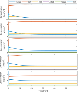
Figure 4: Evolution of the solid concentration in the calciner. The calciner is divided into 5 finite volumes. The top plot is the finite volume in the top of the calciner, while the bottom plot is the finite volume in the bottom of the calciner.

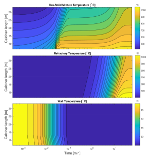
Figure 5: The temperature of the of the gas solid mixture, the refractory temperature, and wall temperature during the 60 min operation of the calciner. The temperatures are illustrated as function of position and time. Note that the time axis is logarithmic.

4.2 Dynamic simulation

Fig. 4 and Fig. 5 illustrate the dynamic behavior of the model. Fig. 4 shows the solid molar concentrations and Fig. 5 shows the temperatures. In this simulation, the system settles to a steady state in 30-40 min. The mixture and refractory wall temperatures increase rapidly from 400^∘C to 900-1000^∘C along the calciner. Right after the ignition point at 1.6 s, the model exhibit non-monotonic behavior. Otherwise the behavior is monotonic approaching the steady states. The calcination process occurs when sufficient heat is released by the combustion.

4.3 Steady-state simulation

Fig. 6 shows the steady-state mass flow of all compounds in the calciner. The calcination process occurs rapidly within the first 10 m where most of the CaO is produced. Similarly, the combustion produces CO from the fuel in the lower part of the calciner. This CO is subsequently consumed in the CO2 forming reactions. The CaCO3 conversion were obtained by manual calibration of the model parameters. The gas compositions can be used to evaluate the qualitative correctness of the steady states. Typical practical operations conditions would be about $35\%$ CO2 and about $3\%$ O2 with the rest being primarily N2. The model produced the steady-state outlet composition: 37.17% CO2, 59.74% N2, 1.42% O2, 0.77% Ar, 0.00% CO, 0.00%C, 0.82% H2O, and 0.08% H2. Hence the fuel is completely consumed and that the level of CO2 is in the right range (slightly higher than the practical operation). Correspondingly, the O2 level is also in the right range (slightly lower than the practical operation).

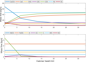
Figure 6: The steady-state mass flows of gasses and solids along the height of the calciner. Most of the calcination occurs in the first 10 m of the calciner.

5 Conclusion

In this paper we presented an index-1 DAE model for the calciner in the pyro-section of a cement plant. The model can be used for dynamical and steady-state simulation of the calciner. By manual calibration, the model is able to provide simulation results that qualitatively matches practical operation. The model is the result of a systematic modeling procedure that involves flow pattern, geometry, thermo-physical properties, transport-phenomena, stoichiometry and kinetics, mass and energy balances, and algebraic relations for the volume and the internal energy. The calciner model will be connected with models for the pre-heating cyclones, the rotary kiln, and the cooler such that the pyro-section of a cement plant can be dynamically simulated. Such a model is important for model-based design and development of control and optimization systems for the pyro-section of cement plants.

Appendix A Physical properties

Table 1-4 provide the parameters and physical properties. Table 1 shows the parameters for the kinetic expressions. Table 2 and Table 3 shows literature data for the solid and gas material properties.

The molar heat capacity of CaCO3 is (Jacobs et al., 1981)

$$\begin{split}c_{p}&=-184.79+0.32\cdot 10^{-3}T-0.13\cdot 10^{-5}T^{2}\\ &-3.69\cdot 10^{6}T^{-2}+3883.5T^{-\frac{1}{2}}\qquad[\frac{\text{J}}{\text{mol}\cdot\text{K}}]\end{split}$$ (36)

for 298-750 K.

The specific heat capacities of the remaining components are computed by (Svensen et al., 2024)

$$c_{p}=C_{0}+C_{1}T+C_{2}T^{2}$$ (37)

and Table 4 reports the corresponding parameters ($C_{0}$, $C_{1}$,$C_{2}$).

Table 1: Reaction rate coefficients of gasses from the open literature.

	Unit	$k_{r}$	n	$E_{A}$	$\alpha_{1}$	$\alpha_{2}$	$\alpha_{3}$	$\beta_{2}$
$r_{1}$a	$\frac{\text{kg}}{\text{m}^{3}s}$	$10^{8}$	0	$175.7$	$1$	$0$	0	0
$r_{2}$a	$\frac{\text{kg}}{\text{m}^{3}s}$	$10^{7}$	0	$240$	$2$	$1$	0	0
$r_{3}$a	$\frac{\text{kg}}{\text{m}^{3}s}$	$10^{9}$	0	$420$	$1$	$1$	0	0
$r_{4}$a	$\frac{\text{kg}}{\text{m}^{3}s}$	$10^{8}$	0	$310$	$3$	$1$	0	0
$r_{5}$a	$\frac{\text{kg}}{\text{m}^{3}s}$	$10^{8}$	0	$330$	$4$	$1$	$1$	0
$r_{6}$b	$\frac{\text{kg}}{\text{m}^{3}s}$	$7.0\cdot 10^{4}$	0	$66.5$	$1$	$1$	0	0
$r_{7}$c	$\frac{\text{mol}}{\text{m}^{3}s}$	$2.8\cdot 10^{6}$	0	83.7	1	1	0	0
$r_{8}$d	$\frac{\text{mol}}{\text{m}^{3}s}$	$1.4\cdot 10^{6}$	0.5	$295.5$	1	1	0	0
$r_{9}$e	$\frac{\text{mol}}{\text{m}^{3}s}$	$8.8\cdot 10^{11}$	0	239	$0.5$	$0.5$	0	0
$r_{10}$f	$\frac{1}{\text{s}}$	$2.6\cdot 10^{8}$	0	237	0	0	0	0.6
$r_{11}$f	$\frac{1}{\text{s}}$	$3.1\cdot 10^{6}$	0	215	0	0	0	0.4

All $\beta_{1},\beta_{3}$ is zero and the unit of the activation energy $E_{A}$ is $[\frac{\text{kJ}}{\text{mol}}]$, ¹ Unclear in source, ^a Mastorakos et al. (1999), ^b Guo et al. (2003), ^c Jones and Lindstedt (1988), ^d Karkach and Osherov (1999), ^eWalker (1985), ^fBasu (2018)

Table 2: Material properties of the solids.

	Thermal Conductivity	Density	Molar mass
Units	$\frac{\text{W}}{\text{K}\cdot\text{m}}$	$\frac{\text{g}}{\text{cm}^{3}}$	$\frac{\text{g}}{\text{mol}}$
CaCO_3	2.248a	2.71b	100.09b
CaO	30.1c	3.34b	56.08b
SiO_2	1.4a,c	2.65b	60.09b
Al_2O_3	12-38.5c 36a	3.99b	101.96b
Fe_2O_3	0.3-0.37c	5.25b	159.69b
C2S	3.45$\pm$0.2d	3.31d	$172.24^{g}$
C3S	3.35$\pm$0.3d	3.13d	228.32b
C3A	3.74$\pm$0.2e	3.04b	270.19b
C4AF	3.17$\pm$0.2e	3.7-3.9f	$485.97^{g}$

^a from Green and Perry (2008), ^b from Rumble (2022),
^c from Ichim et al. (2018), ^d from Abdolhosseini Qomi et al. (2015), ^e from Du and Ge (2021), ^f from Bye (1999),
^g Computed from the above results

Table 3: Material properties of the gasses.

	Thermal Conductivitya	Molar massa	Viscositya	diffusion Volumeb
Units	$\frac{10^{-3}\text{W}}{\text{K}\cdot\text{m}}$	$\frac{\text{g}}{\text{mol}}$	$\mu\text{Pa}\cdot\text{s}$	cm3
CO_2	16.77 (300K) 70.78 (1000K)	44.01	15.0 (T=300K) 41.18 (1000K)	16.3
N_2	25.97(300K) 65.36(1000K)	28.014	17.89(300K) 41.54(1000K)	18.5
O_2	26.49(300K) 71.55(1000K)	31.998	20.65 (300K) 49.12 (1000K)	16.3
Ar	17.84 (300K) 43.58 (1000K)	39.948	22.74(300K) 55.69(1000K)	16.2
CO	25(300K) 43.2(600K)	28.010	17.8(300K) 29.1(1000K)	18
C_sus	-	12.011	-	15.9
H_2O	609.50(300K) 95.877(1000K)	18.015	853.74(300K) 37.615(1000K)	13.1
H_2	193.1 (300K) 459.7 (1000K)	2.016	8.938(300K) 20.73 (1000K)	6.12

^a from Rumble (2022), ^b from Poling et al. (2001)

Table 4: Molar heat capacities.

	$C_{0}$	$C_{1}$	$C_{2}$	Temperature range
Units	$\frac{\text{J}}{\text{mol}\cdot\text{K}}$	$\frac{10^{-3}\text{J}}{\text{mol}\cdot\text{K}^{2}}$	$\frac{10^{-5}\text{J}}{\text{mol}\cdot\text{K}^{3}}$	K
CaOb	71.69	-3.08	0.22	200 - 1800
SiO_2b	58.91	5.02	0	844 - 1800
Al_2O_3b	233.004	-19.59	0.94	200 - 1800
Fe_2O_3c	103.9	0	0	-
C2Sb	199.6	0	0	1650 - 1800
C3Sb	333.92	-2.33	0	200 - 1800
C3Ab	260.58	9.58/2	0	298 - 1800
C4AFb	374.43	36.4	0	298 - 1863
CO_2a	25.98	43.61	-1.49	298 - 1500
N_2a	27.31	5.19	-1.55e-04	298 - 1500
O_2a	25.82	12.63	-0.36	298 - 1100
Ara	20.79	0	0	298 - 1500
COa	26.87	6.94	-0.08	298 - 1500
C_susa	-0.45	35.53	-1.31	298 - 1500
H_2Oa	30.89	7.86	0.25	298 - 1300
H_2a	28.95	-0.58	0.19	298 - 1500

^a coefficient from Jacobs et al. (1981), ^b coefficients from Hanein et al. (2020), ^c from Rumble (2022)

References

- Abdolhosseini Qomi et al. (2015) Abdolhosseini Qomi, M.J., Ulm, F.J., and Pellenq, R.J.M. (2015). Physical origins of thermal properties of cement paste. Phys. Rev. Appl., 3, 064010.
- Alberti et al. (2018) Alberti, M., Weber, R., and Mancini, M. (2018). Gray gas emissivities for H2O-CO2-CO-N2 mixtures. J. Quant Spectrosc Radiat Transf, 219, 274–291.
- Basu (2018) Basu, P. (2018). Chapter 7 - Gasification Theory. In Biomass Gasification, Pyrolysis and Torrefaction, 211–262. Academic Press, 3rd edition.
- Bye (1999) Bye, G.C. (ed.) (1999). Portland Cement: Composition, Production and Properties. Thomas Telford, 2nd edition.
- Du and Ge (2021) Du, Y. and Ge, Y. (2021). Multiphase model for predicting the thermal conductivity of cement paste and its applications. Materials, 14(16).
- Green and Perry (2008) Green, D.W. and Perry, R.H. (eds.) (2008). Perry’s Chemical Engineers’ Handbook. McGraw Hill, 8th edition.
- Guo et al. (2003) Guo, Y., Chan, C., and Lau, K. (2003). Numerical studies of pulverized coal combustion in a tubular coal combustor with slanted oxygen jet. Fuel, 82, 893–907.
- Hanein et al. (2017) Hanein, T., Glasser, F.P., and Bannerman, M.N. (2017). One-dimensional steady-state thermal model for rotary kilns used in the manufacture of cement. Adv. Appl. Ceram., 116(4), 207–215.
- Hanein et al. (2020) Hanein, T., Glasser, F.P., and Bannerman, M.N. (2020). Thermodynamic data for cement clinkering. Cement and Concrete Research, 132, 106043.
- Hesselgreaves et al. (2017) Hesselgreaves, J.E., Law, R., and Reay, D.A. (2017). Chapter 1 - Introduction. In Compact Heat Exchangers, 1–33. Butterworth-Heinemann, 2nd edition.
- Howell and Weathers (1970) Howell, G.W. and Weathers, T.M. (1970). Aerospace Fluid Component Designers’ Handbook. Volume I, Revision D. TRW Systems Group.
- Ichim et al. (2018) Ichim, A., Teodoriu, C., and Falcone, G. (2018). Estimation of cement thermal properties through the three-phase model with application to geothermal wells. Energies, 11(10).
- Iliuta et al. (2002) Iliuta, I., Dam-Johansen, K., and Jensen, L. (2002). Mathematical modeling of an in-line low-nox calciner. Chemical Engineering Science, 57(5), 805–820.
- Incropera et al. (2007) Incropera, F., DeWitt, D., Bergman, T., and Lavine, A. (2007). Fundamentals of Heat and Mass Transfer. John Wiley & Sons.
- Jacobs et al. (1981) Jacobs, G.K., Kerrick, D.M., and Krupka, K.M. (1981). The high-temperature heat capacity of natural calcite (CaCO3). Physics and Chemistry of Minerals, 7, 55–59.
- Johansson et al. (2011) Johansson, R., Leckner, B., Andersson, K., and Johnsson, F. (2011). Account for variations in the \ceH2O to \ceCO2 molar ratio when modelling gaseous radiative heat transfer with the weighted-sum-of-grey-gases model. Combustion and Flame, 158, 893–901.
- Jones and Lindstedt (1988) Jones, W.P. and Lindstedt, R.P. (1988). Global reaction schemes for hydrocarbon combustion. Combustion and Flame, 73, 233–249.
- Kahawalage et al. (2017) Kahawalage, A.C., Melaaen, M.C., and Tokheim, L.A. (2017). Numerical modeling of the calcination process in a cement kiln system. In Proceedings of the 58th SIMS, 83–89.
- Karkach and Osherov (1999) Karkach, S.P. and Osherov, V.I. (1999). Ab initio analysis of the transition states on the lowest triplet \ceH2O2 potential surface. The Journal of Chemical Physics, 110(24), 11918–11927.
- Lehne and Preston (2018) Lehne, J. and Preston, F. (2018). Making concrete change: Innovation in low-carbon cement and concrete. Technical report, Chatham House.
- Mastorakos et al. (1999) Mastorakos, E., Massias, A., Tsakiroglou, C.D., Goussis, D.A., Burganos, V.N., and Payatakes, A.C. (1999). CFD predictions for cement kilns including flame modelling, heat transfer and clinker chemistry. Applied Mathematical Modelling, 23, 55–76.
- Mujumdar et al. (2007) Mujumdar, K.S., Ganesh, K., Kulkarni, S.B., and Ranade, V.V. (2007). Rotary cement kiln simulator (rocks): Integrated modeling of pre-heater, calciner, kiln and clinker cooler. Chem. Eng. Sci., 62(9), 2590–2607.
- Poling et al. (2001) Poling, B.E., Prausnitz, J.M., and O’Connel, J.P. (2001). The Properties of Gases and Liquids. McGraw-Hill.
- Rumble (2022) Rumble, J. (ed.) (2022). CRC handbook of chemistry and physics. CRC Press, 103th edition.
- Sutherland (1893) Sutherland, W. (1893). The Viscosity of Gases and Molecular Force. Philos Mag series 5, 36(223), 507–531.
- Svensen et al. (2024) Svensen, J.L., da Silva, W.R.L., Merino, J.P., Sampath, D., and Jørgensen, J.B. (2024). A dynamical simulation model of a cement clinker rotary kiln. In European Control Conference 2024.
- Toda and Furuse (2006) Toda, K. and Furuse, H. (2006). Extension of Einstein’s viscosity equation to that for concentrated dispersions of solutes and particles. J. Biosci. Bioeng., 102(6), 524–528.
- Walker (1985) Walker, P.L. (1985). Char Properties and Gasification, 485–509. Springer Netherlands.
- Wilke (1950) Wilke, C.R. (1950). A viscosity equation for gas mixtures. The Journal of Chemical Physics, 18(4), 517–519.