Exact Sampling of Spanning Trees
via Fast-forwarded Random Walks

Abstract

Tree graphs are routinely used in statistics. When estimating a Bayesian model with a tree component, sampling the posterior remains a core difficulty. Existing Markov chain Monte Carlo methods tend to rely on local moves, often leading to poor mixing. A promising approach is to instead directly sample spanning trees on an auxiliary graph. Current spanning tree samplers, such as the celebrated Aldous–Broder algorithm, predominantly rely on simulating random walks that are required to visit all the nodes of the graph. Such algorithms are prone to getting stuck in certain sub-graphs. We formalize this phenomenon using the bottlenecks in the random walk’s transition probability matrix. We then propose a novel fast-forwarded cover algorithm that can break free from bottlenecks. The core idea is a marginalization argument that leads to a closed-form expression which allows for fast-forwarding to the event of visiting a new node. Unlike many existing approximation algorithms, our algorithm yields exact samples. We demonstrate the enhanced efficiency of the fast-forwarded cover algorithm, and illustrate its application in fitting a Bayesian dendrogram model on a Massachusetts crimes and communities dataset.

section Introduction

Tree graphs are commonly encountered in statistical modeling. An undirected tree is an acyclic and connected graph $T=(V_{T},E_{T})$ with nodes $V_{T}=(1,\ldots,m)$ and edges $E_{T}=\{(j,l)\}$ with $|E_{T}|=m-1$. By designating a node $r\in V_{T}$ as the root, one can easily obtain from $T$ a directed tree $\vec{T}=(V_{\vec{T}},E_{\vec{T}},r)$, with identical node set $V_{\vec{T}}=V_{T}$ and directed edges $E_{\vec{T}}=\{(j\to l)\}$ obtained from $E_{T}$ by pointing edges away from $r$. Such tree structures provide succinct ways to capture complex dependencies that arise from a wide range of statistical applications.

In hierarchical modeling, directed trees represent multi-layer dependence structures underlying the observed data. From a generative perspective, we consider a $\vec{T}$ where each node $v$ is equipped with a parameter $\mu_{v}$. Using this tree, we define a joint probability distribution for data $y_{1},\ldots,y_{n}$ and parameters $\mu_{1},\ldots,\mu_{m}$ conditioned on assignment labels $z_{i}\in(1,\ldots,m)$:

$$L(y,\mu\mid\vec{T},z)=\Big{\{}\prod_{i=1}^{n}\mathcal{F}(y_{i}\mid\mu_{z_{i}})\Big{\}}\Big{\{}\mathcal{R}(\mu_{r})\prod_{(j\to l)\in E_{\vec{T}}}\mathcal{H}(\mu_{l}\mid\mu_{j})\Big{\}},$$ (equation)

where $\mathcal{H}(\mu_{l}\mid\mu_{j})$ is the transition probability kernel from $\mu_{j}$ to $\mu_{l}$, $\mathcal{R}(\mu_{r})$ is the marginal kernel for $\mu_{r}$ in the root, and $\mathcal{F}$ is the conditional kernel of the data $y_{i}$ given the assignment $z_{i}$ for that observation. There are potentially other parameters characterizing $\mathcal{F}$ and $\mathcal{H}$, including dependence on covariates via decision trees (Chipman et al., 1998; Castillo & Ročková, 2021) or related ensemble methods (Chipman et al., 2010; Linero & Yang, 2018), but we suppress these temporarily for ease of notation. Model (equation) induces a partition on $(1,\ldots,n)$ via the latent assignments $z$. In contrast to traditional mixture models, which often assume the $\mu_{k}$’s to be generated independently from a common distribution, (equation) characterizes dependence in $\mu_{j}$ and $\mu_{l}$ through an ancestry tree. Ancestors of $v$ include the tree nodes in the path from the root to $v$. This type of dependence is well motivated in many application areas. The tree can be interpreted as an inferred evolutionary/phylogenetic history in certain biological settings (Huelsenbeck & Ronquist, 2001; Suchard et al., 2001; Neal, 2003), or alternatively as a multi-layer partitioning of a dataset (Heller & Ghahramani, 2005).

It is also common to use a collection, or forest, of trees for flexibility in modeling. Consider

$$L(y\mid\vec{T}_{1},\ldots,\vec{T}_{K})=\prod_{k=1}^{K}\bigg{\{}\mathcal{R}(y_{r^{(k)}})\prod_{(j\to l)\in E_{\vec{T}_{k}}}\mathcal{H}(y_{l}\mid y_{j})\bigg{\}},$$ (equation)

where each $\vec{T}_{k}=\{V_{\vec{T}_{k}},E_{\vec{T}_{k}},r^{(k)}\}$ is a component tree, and $(V_{\vec{T}_{1}},\ldots,V_{\vec{T}_{K}})$ gives a $K$-partition of data index $(1,\ldots,n)$, where $n=\sum_{k=1}^{K}|V_{\vec{T}_{k}}|$. The kernel $\mathcal{R}$ describes how the first point in a group arises, and $\mathcal{H}$ characterizes the conditional dependence of the subsequent points given the previous ones. The use of trees and forests in graphical modeling (Lauritzen, 2011) dates back at least to the single-linkage clustering algorithm (Gower & Ross, 1969), and is recently seen in dependence graph estimation (Duan & Dunson, 2023), contiguous spatial partitioning (Teixeira et al., 2019; Luo et al., 2021, 2023), and model-based spectral clustering (Duan & Roy, 2023). In addition, likelihood (equation) has been extended to a mixture of overlapping trees in Bayesian network estimation (Meilă & Jordan, 2000; Meilă & Jaakkola, 2006; Elidan & Gould, 2008).

While there is a rich literature on algorithmic approaches for obtaining point estimates of tree graphs (Prim, 1957; Kruskal, 1956), we are particularly interested in model-based Bayesian approaches. Such methods have the advantage of providing a characterization of uncertainty in estimating trees, while also inferring a generative probability model for the data. Uncertainty quantification is crucial in this context. Algorithms that produce a single tree estimate are ripe for over-interpretation and lack of reproducibility, since in most applications there are many different trees that are almost equally plausible for the data. Naturally, the success of such a Bayesian approach hinges on whether one can conduct inferences based on the posterior distribution of trees in a computationally efficient way.

Sampling from posterior distributions for trees is generally a difficult problem. Current Markov chain Monte Carlo samplers often navigate tree spaces using local modifications, such as pruning and growing moves. Since tree spaces are combinatorial and large in size, these samplers often exhibit poor mixing. A natural alternative is to rely on conjugacy to employ block updates on $\vec{T}$ in Gibbs-type samplers. Our strategy is to view $\vec{T}$ as a spanning tree $\vec{\mathcal{T}}$ under a complete and weighted auxiliary graph $G=(V_{G},E_{G})$. Here a spanning tree $\vec{\mathcal{T}}$ of $G$ is simply a subtree of $G$ that spans all the nodes of $G$ with edges oriented away from some root node $r$. For the generative process in (equation), one can consider a complete graph $G$ with nodes $(1,\ldots,m)$, with weighted adjacency matrix $Q\in[0,\infty)^{m\times m}$ of elements $q_{j,l}=\mathcal{H}(\mu_{l}\mid\mu_{j})$ for every pair $(j,l)$. Observing that equation (equation) can be written as $L(y;\mu\mid\vec{T},z)=\mathcal{R}(\mu_{r})\prod_{(j\to l)\in E_{\vec{T}}}\Big{\{}\prod_{z_{i}=l}\mathcal{F}(y_{i}\mid\mu_{z_{i}})\mathcal{H}(\mu_{l}\mid\mu_{j})\Big{\}}$, a natural prior distribution on the tree structure of $\vec{\mathcal{T}}$ arises:

$$\text{Pr}(\vec{\mathcal{T}}|r)\propto\rho_{r}\prod_{(j\to l)\in E_{\vec{\mathcal{T}}}}q_{j,l},$$ (equation)

where $\text{Pr}(r)$ is a discrete probability on $(1,\ldots,m)$, and $\rho_{r}$ is inversely proportional to the normalizing constant $\sum_{\vec{\mathcal{T}}\text{ rooted at }r}\prod_{(j\to l)\in E_{\vec{\mathcal{T}}}}q_{j,l}$, which could vary with $r$ for directed trees. The resulting posterior distribution on $\vec{\mathcal{T}}$ shares a conjugate product-over-edges form with the prior $\text{Pr}(\vec{\mathcal{T}})$ under the likelihood. The core imperative, then, is to efficiently sample from spanning tree distributions of the form (equation). Notably, the uniform spanning tree distribution is a special case of (equation).

The celebrated Aldous–Broder algorithm (Aldous, 1990; Broder, 1989) provides a tractable way to draw exact samples from (equation). The algorithm proceeds by taking a random walk $X_{t}=(r,x_{1},x_{2},\ldots,x_{t})$ on $V_{G}$ and stops at the cover time of the walk when all nodes have been visited. By collecting the first entrance edges of $X_{t}$, which are the set of edges via which the walk first visited each node, one obtains a spanning tree $\vec{\mathcal{T}}$ rooted at $r$. By separately specifying a distribution over the root node $r$, one obtains a distribution on the directed spanning trees $\vec{\mathcal{T}}$. For a graph $G$ containing $m$ nodes, Broder & Karlin (1989) shows an expected cover time of $O(m\log m)$ in well-connected graphs and $O(m^{3})$ in the worst case.

The Aldous–Broder algorithm can be empirically slow. In practice, even if the number of nodes $m$ in $G$ is small, the algorithm can get stuck in certain subgraphs for a long time. This issue is inherent to the nature of random walks. Other popular algorithms, such as Wilson’s algorithm based on the loop-erased random walk (Wilson, 1996), also suffer from the same problem.

We formalize this pathological phenomenon using eigenvalues of a normalized Laplacian to characterize bottlenecks in the graph. We then propose a fast-forwarded cover algorithm for exact sampling from the distribution in (equation) while bypassing wasteful random walk steps. The key observation is that we do not need to simulate the entire random walk trajectory to obtain the first entrance edges to each node. We derive a closed form expression that allows for direct, fast-forwarded sampling of these first entrance edges via a marginalization argument. This algorithm leads to dramatically faster performance in simulations in the presence of bottlenecks.

Existing spanning tree samplers often perform transitions directly according to the underlying graph’s adjacency matrix $Q$, restricting their applicability to symmetric/undirected cases. We show that by using an auxiliary matrix $W$, which is generated from $Q$ under certain transformations, to specify the random walk transition probabilities, our fast-forwarded cover algorithm can be extended to more general scenarios, including cases where the underlying graph has an asymmetric adjacency matrix or the induced Markov chains are irreversible. These results are of independent interest. We illustrate our sampler by fitting a Bayesian dendrogram model on a Massachusetts crimes and communities dataset. The resulting Gibbs sampler exhibits drastically improved mixing performance compared to a reversible jump sampler based on local moves.

section Method

section.subsection Background on Aldous–Broder Algorithm

We review and summarize results on the Aldous–Broder algorithm (Aldous, 1990; Broder, 1989) in this section. This algorithm samples a random spanning tree $\vec{\mathcal{T}}$ from the underlying graph $G$ based on a random walk. Consider a weight matrix $W\in[0,\infty)^{m\times m}$ which is used to specify the random walk transition probabilities on $G$. For simplicity, it suffices for now to consider $W$ as the graph’s weighted adjacency matrix $Q$ in (equation), an important special case that applies when $Q$ is symmetric. However, our results hold for more general cases where the transition matrix $W$ is some specific transformation of $Q$. A detailed discussion is in Section 2.4.

We use $W$ to specify a random walk over the state space $V_{G}=(1,\ldots,m)$. This random walk is a discrete-time Markov chain $X=(x_{0},x_{1},\ldots)$ with transition probabilities:

$$p_{j,l}=\textup{Pr}(x_{t+1}=l\mid x_{t}=j)=\frac{w_{j,l}}{d_{j}},\qquad d_{j}=\sum_{v=1}^{m}w_{j,v},$$ (equation)

where $d_{j}>0$ and $w$ denotes entries of $W$. We assume the Markov chain is irreducible: for any pair of $(j,l)$, there exists $t>0$ such that $\textup{Pr}(x_{t}=l\mid x_{0}=j)>0$. We denote the random walk up to time $t$ by $X_{t}=(x_{0},x_{1},\ldots,x_{t})$, and the invariant distribution of $x_{t}:t\to\infty$ by $(\pi_{1},\ldots,\pi_{m})$. The result of Broder (1989) further assumes reversibility of the Markov chain, $\pi_{j}p_{j,l}=\pi_{l}p_{l,j}$; however, this condition is not needed here.

The Aldous–Broder algorithm proceeds as follows: initialize the walk $x_{0}$ at root $r$; perform the random walk until all nodes are visited at the cover time $\hat{t}$; construct a directed spanning tree $\vec{\mathcal{T}}$ with the edge set as the set of first-entrance edges all pointed away from $r$. Formally,

$$E_{\vec{\mathcal{T}}}=\bigcup_{j\in(V_{G}\setminus r)}\Big{\{}(x_{(t_{j}-1)}\to x_{t_{j}}):t_{j}=\min_{1\leq t\leq\hat{t}}(t:x_{t}=j)\Big{\}}.$$ (equation)

The following theorem characterizes the induced distribution of ${\vec{\mathcal{T}}}$.

Theorem section.theorem (Extended Aldous–Broder).

Letting ${\vec{\mathcal{T}}}$ be generated as above, then

$$\textup{Pr}({\vec{\mathcal{T}}}\mid r)\propto\Big{\{}\prod_{(j\to l)\in E_{\vec{\mathcal{T}}}}\frac{p_{j,l}\pi_{j}}{\pi_{l}}\Big{\}}\frac{1}{\pi_{r}}\propto\prod_{(j\to l)\in E_{\vec{\mathcal{T}}}}({p_{j,l}\pi_{j}}),$$ (equation)

where the probability is normalized over all ${\vec{\mathcal{T}}}$ rooted from $r$.

The first term in (equation) is based on an adaptation of Theorem 3 of Fredes & Marckert (2023), where a directed tree with edges pointed towards the root is used, as is standard in the probability literature. While this is the opposite of our choice of orientation, the mathematical results carry over. The second term is based on the fact that $\{\prod_{(j\to l)\in E_{\vec{\mathcal{T}}}}{\pi_{l}}\}\pi_{r}=\prod_{j=1}^{m}\pi_{j}$, which is invariant to $E_{{\vec{\mathcal{T}}}}$ and hence can be omitted.

In Section 2.4, we describe how one can choose $W$ as some appropriate transformation of $Q$ so that (equation) becomes the product form shown in (equation) under general settings without requiring matrix symmetry for $W$. For now in Section 2.2, we focus on computational aspects and discuss bottleneck effects that impact the cover time of the Aldous–Broder algorithm.

section.subsection Bottlenecks in Random Walk Cover Algorithm

The Aldous–Broder algorithm is only efficient if there is a small cover time $\hat{t}$ to reach all nodes in $V_{G}$. However, when there are bottlenecks in the graph that lead to close-to-zero probabilities to move from the visited nodes $U$ to the unvisited nodes $\bar{U}=V_{G}\setminus U$, the random walk can spend a long time within $U$. We now characterize the consequences from this curse of bottlenecks.

Figure figure illustrates three common challenges through example graphs. The first two graphs are either directed or undirected, while the third is directed. First, as in panel (a), there may be disjoint sets of nodes that are only weakly connected, in the sense that the transition probability between sets are small. Second, as in panel (b), there may be nodes that are isolated with few edges incident to them, and each edge having low transition probability. In this case, the random walk cover algorithm may visit most of nodes within a short time, but faces difficulties reaching the last few. Third, as in panel (c), in a directed graph, due to edge weight asymmetry, there may be a much higher probability to remain in a node set that has been visited.

Regardless of the specific scenario, the curse of bottlenecks can be understood as a close-to-zero probability to move to the unvisited set, marginalized over both the current node and the potential arrival node amongst unvisited nodes.

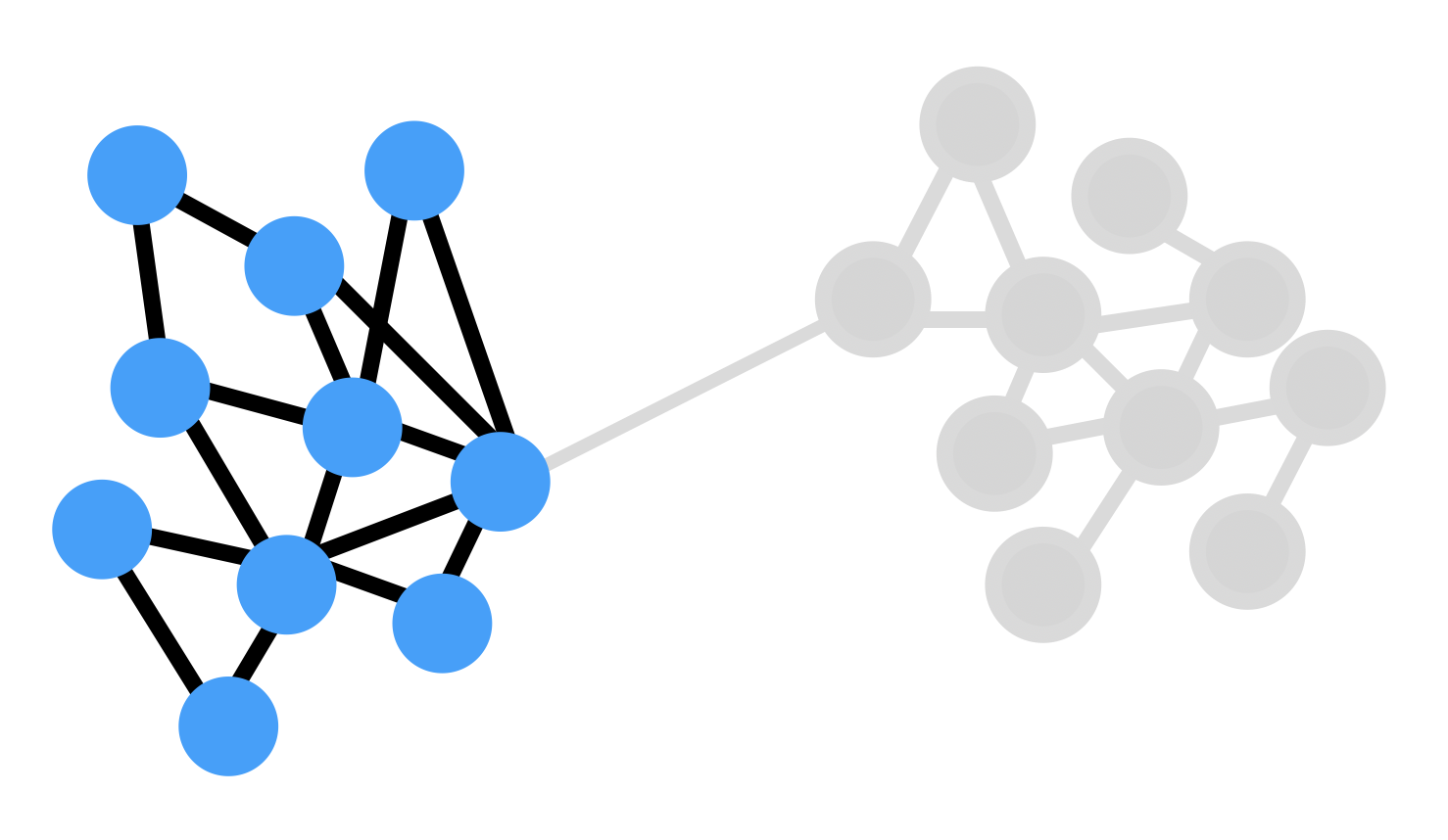
(a) Low edge weight between visited nodes (blue) and unvisited (grey).

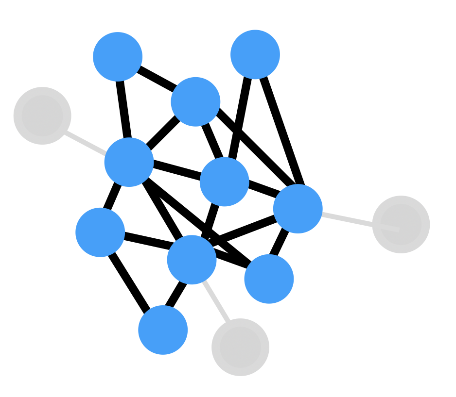
(b) Unvisited nodes (grey) that are isolated.

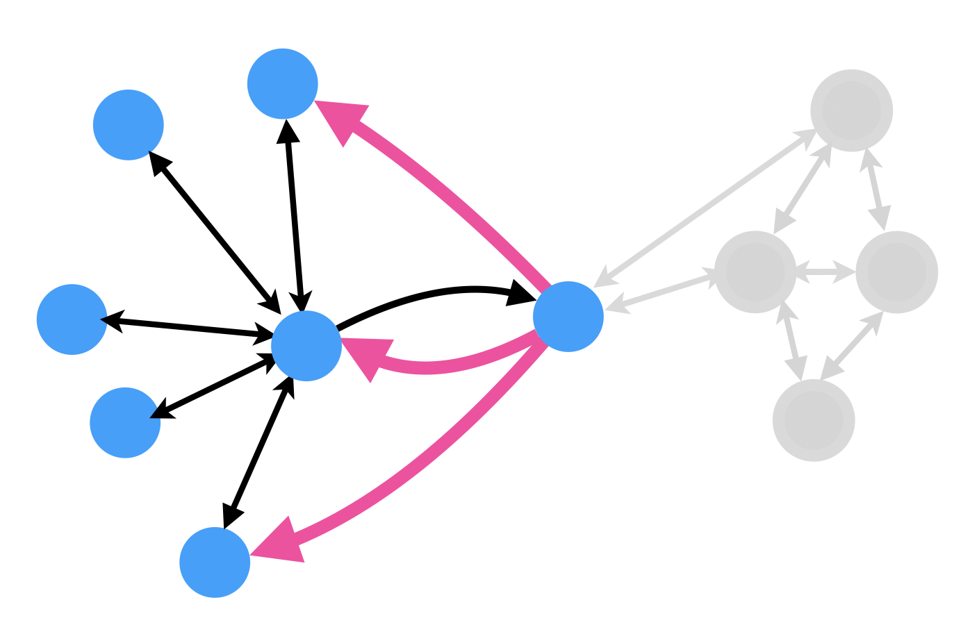
(c) Large probability (magenta lines) to return to visited nodes (blue) in a directed graph.

Figure figure: Illustration of some commonly encountered graphs with curse of bottlenecks — a low transition probability to move from the visited nodes (blue) to those unvisited (grey).

We now formally characterize this phenomenon. Consider a strictly increasing node set $(r)=U_{1}\subset U_{2}\subset\ldots\subset U_{m}=V_{G}$, recording the history of visited nodes by the random walk, with $U_{k}=\cap_{t=0}^{\hat{t}_{k}}X_{t}$ and $\hat{t}_{k}=\min(t\geq 0:|\cap_{\tilde{t}=0}^{t}X_{\tilde{t}}|=k),$ where we refer to $\hat{t}_{k}$ as the partial cover time for $k$ nodes. The probability of transitioning outside of $U_{k}$ at time $t+1$, conditional on the walk remaining within $U_{k}$ from the beginning through time $t$ is

$$\text{Pr}(x_{t+1}\in\bar{U}_{k}\mid x_{t}\in U_{k}) =\sum_{j\in U_{k}}\bigg{\{}\frac{\sum_{l\in\bar{U}_{k}}w_{j,l}}{d_{j}}\text{Pr}(x_{t}=j\mid x_{\tilde{t}\leq t}\in U_{k})\bigg{\}}\leq\max_{j\in U_{k}}\bigg{(}\frac{\sum_{l\in\bar{U}_{k}}w_{j,l}}{d_{j}}\bigg{)}$$

$$=\bigg{(}{\min_{j\in U_{k}}\frac{\sum_{l^{\prime}\in U_{k}}w_{j,l^{\prime}}}{\sum_{l\in\bar{U}_{k}}w_{j,l}}+1}\bigg{)}^{-1},$$

where the inequality uses the fact that the weighted average over $j\in U_{k}$ is less than or equal to the maximum, and the last equality is based on decomposing $d_{j}=\sum_{l\in\bar{U}_{k}}w_{j,l}+\sum_{l^{\prime}\in U_{k}}w_{j,l^{\prime}}$. Therefore, if the total outgoing weights to $\bar{U}_{k}$ are dominated by the weights of staying within $U_{k}$, in the sense that ${\sum_{l\in\bar{U}_{k}}w_{j,l}}\ll{\sum_{l^{\prime}\in U_{k}}w_{j,l^{\prime}}}$, it is unlikely that $x_{t+1}\in\bar{U}_{k}$. With the above ingredients, we are ready to quantify the expected cover time.

Theorem section.theorem.

For a history of visited nodes $(U_{1},\ldots,U_{m})$, the expected cover time $\hat{t}=\hat{t}_{m}$ has

$$\mathbb{E}(\hat{t};U_{1},\ldots,U_{m})\geq(m-1)+\sum_{k=1}^{m-1}\min_{j\in U_{k}}\frac{\sum_{l^{\prime}\in U_{k}}w_{j,l^{\prime}}}{\sum_{l\in\bar{U}_{k}}w_{j,l}}.$$

Remark section.theorem.

The lower bound applies to any $W\in[0,\infty)^{m\times m}$ that leads to an irreducible Markov chain. In practice, when the random walk cover algorithm appears to be stuck at a certain $U_{k}$, one can directly use $\min_{j\in U_{k}}({\sum_{l^{\prime}\in U_{k}}w_{j,l^{\prime}}})/({\sum_{l\in\bar{U}_{k}}w_{j,l}})$ as an estimate for the expected time to leave.

The above result is a quantification for a specific node history of $(U_{1},\ldots,U_{m})$. One can obtain a worst case expected cover time by maximizing over all possible sequences of $(U_{1},\ldots,U_{m})$. We are chiefly interested in $W$ matrices that satisfy a circulation condition: $\sum_{l=1}^{m}w_{j,l}=\sum_{k=1}^{m}w_{k,j},j=1,\ldots,m$, which includes symmetric $W$ with $w_{j,l}=w_{l,j}$ as a special case.

Theorem section.theorem.

For a random walk $X$ based on weight matrix $W$ satisfying the circulation condition, the worst case expected cover time $\hat{t}$ has

$$\max_{\text{all }(U_{1},\ldots,U_{m})}\mathbb{E}(\hat{t};U_{1},\ldots,U_{m})\geq\frac{1}{M\sqrt{\lambda_{2}(\mathcal{L})}}+m-2,$$

with $M=\sup_{t\geq 0}\sup_{j}\{\text{Pr}(x_{t}=j)/\pi_{j}\}$, and $\lambda_{2}(\mathcal{L})$ the second smallest eigenvalue of the normalized graph Laplacian $\mathcal{L}$.

Remark section.theorem.

Although the above lower bound on expected cover time is inspired by earlier works (Matthews, 1988; Lovász & Winkler, 1993; Levin & Peres, 2017), our result is distinguished by a directly computable lower bound. The constant $M^{-1}$ has a lower bound $\min_{j}\pi_{j}$ for any root distribution for $x_{0}=r$. In the special case where the root node is drawn from the invariant distribution $r\sim\pi$, $M=1$ since $\text{Pr}(x_{t}=j)=\pi_{j}$ for any $t\geq 0$.

section.subsection Skipping Bottlenecks via Fast-forwarding

With the curse of bottlenecks on the cover time of random walks established, we now exploit a useful fact — when transforming the random walk trajectory $X_{\hat{t}}$ into the spanning tree edges $E_{{\vec{\mathcal{T}}}}$, one only needs the first entrance edges to each node. It is unnecessary to simulate entire random walk trajectories until reaching a new node, if the marginal distribution of the next first entrance edge can be directly sampled. We formalize this idea below.

We set up notation here. At any time $t$, suppose we have visited nodes in $U$, and let $e_{j}^{t}=1$ if the walk is at node $j\in U$ at time $t$ and first exits $U$ at time $t+1$. Let $e_{j}^{t}=0$ otherwise. Given a starting location $x_{t_{0}}=j_{0}\in U$ at some time $t_{0}$, drawing the first entrance edge into $\overline{U}$ at $t_{0}+\delta$ for some fixed $\delta\in\mathbb{Z}_{+}$ can be understood as the result of the following events,

$$(e^{t_{0}}_{j_{0}}=0)\Rightarrow(x_{{t_{0}}+1}=j_{1}\in U)\Rightarrow(e^{{t_{0}}+1}_{j_{1}}=0)\Rightarrow\cdots\Rightarrow(x_{{t_{0}}+\delta}=j^{\prime}\in U)\Rightarrow(e^{t_{0}+\delta}_{j^{\prime}}=1).$$

The trajectory of the walk stays within $U$ from time $t_{0}$ until $t_{0}+\delta$ and exits from node $j^{\prime}\in U$ to node $l^{\prime}\in\bar{U}$ at time $t_{0}+\delta+1$. This implies the first-entrance edge $j^{\prime}\to l^{\prime}$. We write

$$\eta_{j}=\text{Pr}(e^{t}_{j}=1),\qquad(1-\eta_{j})=\text{Pr}(e^{t}_{j}=0)=\frac{\sum_{k\in U}w_{j,k}}{d_{j}}.$$

Collecting the $\eta$’s into vector form, $\eta_{U}=(\eta_{j}:j\in U)$. Let $P_{U,U}=\{p_{j,l}:j\in U,l\in U\}$ represent the transition probability matrix from nodes in $U$ back into $U$. Writing a state vector $s_{t}=\{\text{Pr}(x_{t}=j^{\prime}\mid x_{t_{0}}=j_{0})\}_{j^{\prime}\in U}$, we have the recursive relation $s_{t+1}=P_{U,U}^{T}s_{t},$ when the walk has not left $U$ by time $t+1$. The initial state $s_{t_{0}}$ is a $|U|$-dimensional vector with the element corresponding to $j_{0}$ set to $1$ and all others equal to $0$. We then have

$$\text{Pr}(x_{t_{0}+\delta}=\cdot,x_{t_{0}+\delta+1}\in\bar{U}\mid x_{t_{0}}=j_{0})=\text{diag}(\eta_{U})(P_{U,U}^{T})^{\delta-1}s_{t_{0}}.$$

Here, we started at the initial state at time $t_{0}$, transitioned within the visited nodes $U$ for $\delta-1$ times, and visited $\bar{U}$ at time $t+\delta+1$ via $\text{diag}(\eta_{U})$. This expression represents the distribution on the nodes that $x_{t_{0}+\delta}$ can take. We can further marginalize the above by summing over $\delta\in\mathbb{Z}_{\geq 0}$. Since the summation involves a Neumann series, it has a closed-form for the marginal if the series converges. The following theorem shows a sufficient condition.

Theorem section.theorem.

If $P_{U,U}$ is irreducible (cannot be rearranged to a block upper-triangular matrix via row and column permutations), and there exists at least one $j\in U:\eta_{j}>0$, then

$$\textup{Pr}(x_{({{\hat{t}_{|U|+1}}-1)}}=\cdot\mid x_{t_{0}}=j_{0})=\textup{diag}(\eta_{U})(I-P_{U,U}^{T})^{-1}s_{t_{0}},$$ (equation)

where $({{\hat{t}_{|U|+1}}-1})$ is the time point before moving to a node in $\bar{U}$.

The above irreducibility condition is satisfied when $w_{j,l}>0$ for all $j\neq l$. This theorem allows us to sample the first exit edge $(j^{\prime},l^{\prime})$ from $U$ to $\bar{U}$ in a straightforward manner. We first draw $j^{\prime}\in U$ according to the distribution specified by the vector in (equation). We then take one random step from the drawn node $j^{\prime}$ via the transition specified by

$$\text{Pr}(x_{{{\hat{t}_{|U|+1}}}}=l^{\prime}\mid x_{({{\hat{t}_{|U|+1}}-1)}}=j^{\prime},e^{(\hat{t}_{|U|+1}-1)}_{j}=1)={w_{j^{\prime},l^{\prime}}}/{\sum_{k\in\bar{U}}w_{j^{\prime},k}}$$ (equation)

to obtain $l^{\prime}\in\bar{U}$. We refer to steps (equation) and (equation) as the fast-forwarding steps.

Remark section.theorem.

Direct calculation of the matrix inverse $(I-P_{U,U}^{T})^{-1}$ has $O(|U|^{3})$ cost, but solving the linear equation $x:(I-P_{U,U}^{T})x=s_{t_{0}}$ has a low cost $O(\tilde{K}|U|)$ via iterative numerical methods, with $\tilde{K}$ the number of iterations until convergence (Saad, 2003).

A natural algorithm for drawing a spanning tree performs Aldous–Broder type random walk steps until a bottleneck is reached, and then uses fast-forwarding steps; this is then repeated until visiting all nodes. We call this approach the fast-forwarded cover algorithm.

The fast-forwarded cover algorithm.

Initialize $\tau=0$, $x_{\tau}=r$ and initialize the first entrance step tracker $\alpha=0$

1. Set $\tau=1$. Simulate one random walk step to $x_{\tau}$

2. If $x_{\tau}$ has not not been visited before, update $\alpha\leftarrow\tau$.

3. If the steps taken since first entrance step $(\tau-\alpha)\geq\kappa_{0}$, a pre-set threshold,

update $x_{\tau+1}$ to $j^{\prime}$ sampled according to (equation)

update $x_{\tau+2}$ to $l^{\prime}$ sampled according to (equation)

update $\alpha\leftarrow\tau+2$, and $\tau\leftarrow\tau+3$. Go to Step 1.

If $(\tau-\alpha)<\kappa_{0}$, update $\tau\leftarrow\tau+1$. Go to Step 1.

Repeat the above until all $\alpha=m$, where $m$ is the number of nodes of the underlying graph.

Collect and return the first entrance edges.

We use a new index $\tau$ above, since the iteration number will be different from the underlying random walk time index $t$, as soon as a fast-forwarding step is used. The algorithm completes when all nodes have been visited, and the total iterations needed is at most $\kappa_{0}(m-1)$. In this article, we set $\kappa_{0}=1,000$, which leads to excellent performance in all our experiments.

Before presenting our empirical results, we generalize the random walk cover and our fast-forwarded modifications to be broadly applicable to sampling any directed spanning tree with probability in the form of (equation). This is accomplished through a careful specification of the transition matrix $P$, or equivalently $W$ up to row-wise normalization.

section.subsection Generalizing the Applicability of Cover Algorithms

Given a graph with weighted adjacency matrix $Q$, our goal is to draw samples from (equation) using cover algorithms, a terminology we use to include random walk cover and our fast-forwarded modifications. Several cases are of interest.

Case 1, Circulation: We start with the canonical case in which a simple condition $\sum_{l=1}^{m}q_{j,l}=\sum_{k=1}^{m}q_{k,j}$ holds for $j=1,\ldots,m$. If we view $q_{j,l}$ as a flow from node $j$ to $l$, these equalities describe a type of conservation of flow, with $Q$ describing a circulation matrix (Chung, 2005). This includes the special case where $Q$ is symmetric. Under this circulation condition, setting the random walk transition probabilities $w_{j,l}$ as equal to the underlying graph’s edge weights $q_{j,l}$ is sufficient for cover algorithms to produce samples satisfying

$$\textup{Pr}({\vec{\mathcal{T}}}\mid r)\propto\prod_{(j\to l)\in E_{\vec{\mathcal{T}}}}q_{j,l},$$ (equation)

corresponding to $\rho_{r}=1$. Therefore, we can draw the root from $\textup{Pr}(r)$, and use a cover algorithm with $W=Q$ to obtain samples distributed according to (equation).

Case 2, General form: For a general $Q\in[0,\infty)^{m\times m}$, the stationary distribution vector $\pi$ is a deterministic transform of a left eigenvector of the transition probability matrix $P$. Here, $({p_{j,l}\pi_{j}})\propto q_{j,l}$ may not hold for all $(j,l)$. To solve this problem, we introduce an auxiliary Markov chain as a mathematical tool for calculating $P$. Consider a chain $Y=(y_{0},y_{1},\ldots)$ over $V_{G}$ with transition kernel:

$$\tilde{p}_{l,j}=\textup{Pr}(y_{t+1}=j\mid y_{t}=l)=\frac{q^{*}_{l,j}}{\sum_{k=1}^{m}q^{*}_{l,k}},\qquad q^{*}_{l,j}=q_{j,l}.$$

We denote the invariant distribution of $y_{t}:t\to\infty$ by $(\pi^{*}_{1},\ldots,\pi^{*}_{m})$, which can be numerically computed as a left eigenvector of the transition matrix formed by the $\tilde{p}_{l,j}$’s.

We now form the chain $X=(x_{0},x_{1},\ldots)$ with the transition probability specified as:

$$p_{j,l}=\frac{\tilde{p}_{l,j}\pi^{*}_{l}}{\pi^{*}_{j}}.$$ (equation)

Reversibility ($p_{j,l}=\tilde{p}_{j,l}$) is not needed; however, we can see that $\sum_{j}p_{j,l}\pi^{*}_{j}=\pi^{*}_{l}$ for all $l$. Therefore, $X$ has the same invariant distribution $(\pi_{1},\ldots,\pi_{m})=(\pi^{*}_{1},\ldots,\pi^{*}_{m})$ as $Y$. As a result, we can run a cover algorithm using $P$ from (equation). The probability (equation) in Theorem 1 becomes

$$\textup{Pr}({\vec{\mathcal{T}}}\mid r)\propto\prod_{(j\to l)\in E_{\vec{\mathcal{T}}}}(\tilde{p}_{l,j}\pi^{*}_{l})=\prod_{(j\to l)\in E_{\vec{\mathcal{T}}}}\frac{q_{j,l}}{\sum_{k=1}^{m}q_{k,l}}\pi^{*}_{l}\propto\Big{(}\prod_{(j\to l)\in E_{\vec{\mathcal{T}}}}q_{j,l}\Big{)}\Big{(}\frac{\sum_{k=1}^{m}q_{k,r}}{\pi^{*}_{r}}\Big{)},$$ (equation)

using the invariance to ${\vec{\mathcal{T}}}$ implied by ${\pi^{*}_{r}}/({\sum_{k=1}^{m}q_{k,r}})\prod_{(j\to l)\in E_{\vec{\mathcal{T}}}}{\pi^{*}_{l}}/({\sum_{k=1}^{m}q_{k,l}})=\prod_{l=1}^{m}{\pi^{*}_{l}}/({\sum_{k=1}^{m}q_{k,l}})$. The above result involves a non-constant $\rho_{r}=({\sum_{k=1}^{m}q_{k,r}}/{\pi^{*}_{r}})$, as in (equation), which may pose inconveniences when one wants to draw from $\textup{Pr}({\vec{\mathcal{T}}})\propto h_{r}\prod_{(j\to l)\in E_{\vec{\mathcal{T}}}}q_{j,l}$ for some known kernel $h_{r}$. To solve this issue, one can first draw the root from $\textup{Pr}(r)\propto(h_{r}/\rho_{r})$, and then use a cover algorithm to draw from $\textup{Pr}({\vec{\mathcal{T}}}\mid r)$, so that $\rho_{r}$ is effectively canceled.

section Simulations

To investigate the gain in computational efficiency of our fast-forwarded cover algorithm over the random walk cover algorithm, we conduct several simulations and compare their runtime based on R code on an M1-chip laptop.

First, we assess the impact of size of bottlenecks, quantified via $1/\sqrt{\lambda_{2}(\mathcal{L})}$, on wall-clock runtime. We simulate a graph with $500$ nodes, where we partition the nodes $V$ into two blocks with $|V_{1}|=|V_{2}|=250$. The graph is represented by a symmetric weight matrix $W\in\mathbb{R}^{500\times 500}$ with each $w_{j,l}=u_{j,l}b_{j,l}$. The factor $u_{j,l}$ representing the size of the weight is simulated from $\text{Unif}(0,1)$. We set $b_{j,l}=1$ for those $j$ and $l$ that are in the same node partition, and $b_{j,l}\sim\text{Bern}(\zeta)$ for those $j$ and $l$ that are in different partitions. This creates two complete subgraphs connected by a small number of edges having small weight. We conduct experiments under different edge densities with $\zeta$ from $(0.5,0.1,0.05,0.01)$, corresponding to a range of bottleneck values near $1/\sqrt{\lambda_{2}(\mathcal{L})}=(249,560,786,1738)$. Under each value of $\zeta$, we draw 10 spanning trees using random walk cover algorithm, and 10 trees using fast-forwarded cover algorithm. Figure figure(a) shows that the runtime for the random walk algorithm increases rapidly as the bottleneck size increases, while the fast-forwarded algorithm runtime is almost unaffected by bottleneck size. Similar plots are shown in the supplementary materials, where we compare the Aldous–Broder algorithm and the fast-forwarded algorithm in the same setting but in number of iterations.

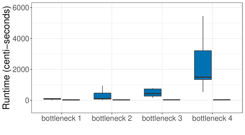
(a) Runtime for different bottlenecks $1/\sqrt{\lambda_{2}(\mathcal{L})}$.

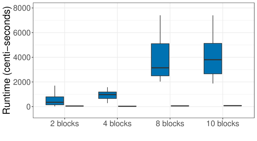
(b) Runtime over different numbers of blocks and hence bottlenecks.

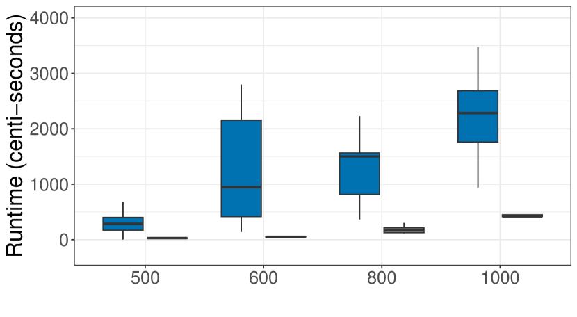
(c) Runtime over different numbers of nodes.

Figure figure: Comparisons of runtime between random walk cover (blue) and fast-forwarded cover (grey) algorithm. In each setting, the fast-forwarded algorithm runtime has a small mean and variance, so that each grey box appears close to a thin line.

Second, we assess effects of the number of blocks on runtime; more blocks implies more bottlenecks. We simulate $W\in\mathbb{R}^{600\times 600}$ according to $w_{j,l}=u_{j,l}b_{j,l}c_{j,l}$. The factors $u_{j,l}$ and $b_{j,l}$ are simulated as above, except we partition the $600$ nodes into $K$ blocks $(V_{1},\ldots,V_{K})$ each of node size $(600/K)$, and use $b_{j,l}=b_{l,j}\sim\text{Bern}(0.001)$ and $c_{j,l}=0.005/K$ for those $(j,l):j\in V_{k},l\in V\setminus V_{k}$. The factors $c_{j,l}$ are chosen so that empirically the size of $1/\sqrt{\lambda_{2}(\mathcal{L})}$ remains roughly the same. We vary $K$ in $(2,4,8,10)$, draw 10 spanning trees using the random walk algorithm, and 10 trees using the fast-forwarded cover algorithm. Figure figure(b) shows that the runtime of random walk cover increases quickly as the number of blocks increases, while the fast-forwarded algorithm is again almost unaffected.

Lastly, we assess scalability for larger numbers of nodes ranging in $(500,600,800,1000)$ in the two block case using $b_{j,l}=b_{l,j}\sim\text{Bern}(0.1)$. Figure figure(c) shows that the runtime for the fast-forwarded cover algorithm increases at an approximately linear rate in node size $m$, while the runtime for the random walk cover algorithm increases much faster.

section Bayesian Dendrogram Inference for Crime and Communities Data

We demonstrate the use of our algorithm in inferring a Bayesian dendrogram. We consider a hierarchical model in the form of (equation) for continuous $y_{i}\in\mathbb{R}^{\tilde{d}}$ with $\vec{T}$ rooted at node 1, and we choose multivariate normal conditional densities as:

$$\mathcal{F}(y_{i}\mid\mu_{z_{i}})=\phi(y_{i};\mu_{z_{i}},\Sigma),\qquad\mathcal{H}(\mu_{l}\mid\mu_{j},\Sigma)=\phi(\mu_{l};\mu_{j},\lambda^{-1}\Sigma).$$

We assign priors $\Pi_{0}(\vec{T})\propto 1$, $z_{i}\stackrel{{\scriptstyle iid}}{{\sim}}\text{Categorical}({\tilde{\pi}}_{1},\ldots,{\tilde{\pi}}_{\tilde{K}})$, $({\tilde{\pi}}_{1},\ldots,{\tilde{\pi}}_{\tilde{K}})\sim\text{Dir}(\alpha,\ldots,\alpha)$, $\Sigma\sim\text{W}^{-1}(\nu,\Sigma_{0})$. Since $\mathcal{F}$ and $\mathcal{H}$ have a shared covariance $\Sigma$ up to a scale shift $\lambda>0$, a conjugate normal-inverse Wishart prior can be chosen for $\mu$ and $\Sigma$.

Our interest is inferring the posterior on $\vec{T}$, but we also have uncertainty in allocations $z_{i}$ and component-specific parameters $(\mu_{k})$. The resulting joint posterior distribution is highly complex. Due to the computational challenges, the literature tends to avoid characterizing uncertainty in $\vec{T}$. For example, for Bayesian hierarchical clustering, Heller & Ghahramani (2005) uses a hypothesis testing criterion to iteratively merge clusters, whereas Heard et al. (2006) combines clusters based on a metric capturing inter-cluster closeness. Alternatively, one can use a Markov chain Monte Carlo sampling algorithm. Classical algorithms rely on making local changes in $\vec{T}$ using reversible-jump Metropolis-Hastings (Chipman et al., 1998; Denison et al., 1998). Such algorithms tend to be very inefficient. Wu et al. (2007) considers adding a move allowing for larger tree restructuring to improve mixing, but with high per iteration expense for large graphs.

Our new spanning tree sampler can be exploited to bypass these computational challenges. We take an overfitted modeling approach, by considering an encompassing tree ${\vec{\mathcal{T}}}$ with $\tilde{m}$ nodes rooted at 1, with $\tilde{m}$ sufficiently large to provide an upper bound on the true value $\tilde{m}\geq m$. This allows us to build a blocked Gibbs sampler based on drawing from $\Pi(z\mid y,\mu,{\vec{\mathcal{T}}})$, $\Pi(\mu\mid y,z,{\vec{\mathcal{T}}})$ and $\Pi({\vec{\mathcal{T}}}\mid\mu)$, with ${\vec{\mathcal{T}}}$ a spanning tree for $\tilde{m}$ nodes, in addition to steps updating other parameters.

After obtaining a posterior sample, we can marginalize out the redundant nodes and change each sampled spanning tree ${\vec{\mathcal{T}}}$ to a reduced dendrogram $\vec{T}$, while maintaining an equivalent generative model for the data. Given a sample of $(z_{1},\ldots,z_{n})$, and $\vec{T}$ initialized at ${\vec{\mathcal{T}}}$, we use the following pruning procedures corresponding to integrating out the densities related to $j$:

• If $j$ is an empty leaf node, without any downstream edge $(j\to l)$ and with $\sum_{i=1}^{n}1(z_{i}=j)=n_{j}=0$, we remove $j$ and $(k\to j)$ from $\vec{T}$.

• If $j$ only has two edges $(k\to j)$ and $(j\to l)$, and $n_{j}=0$, we remove $j$ and replace the two edges by $(k\to l)$ in $\vec{T}$.

We iterate the above pruning steps on the tree’s nodes until we cannot reduce the size of $\vec{T}$ any further. The spanning tree ${\vec{\mathcal{T}}}$ can be viewed as a latent variable that facilitates model specification and posterior computation for the dendrogram $\vec{T}$. We refer to this approach as a spanning tree-augmented dendrogram.

To illustrate this model, we consider an application to the Community and Crimes dataset from the University of California at Irvine Machine Learning Repository. The dataset consists of socioeconomic attributes from the 1990 United States Census, crime statistics from the 1995 Uniform Crime Report, and law enforcement attributes from the 1990 Law Enforcement Management and Administrative Statistics Survey. We focus on economic data from the state of Massachusetts, where there are $n=123$ relevant entries, each corresponding to a community in the state, with ${\tilde{d}}=2$ continuous attributes: the community’s median income and median rent. These attributes are log-transformed and standardized to have sample mean $0$ and marginal sample variance $1$. Our focus is on characterizing variability in these economic attributes by grouping the communities hierarchically. A dendrogram is natural for this purpose.

We choose priors to favor node parameters $\mu_{j}$ that are broadly spread across the support of the data, with relatively few data points associated with each $\mu_{j}$. This is achieved by choosing $\nu=n$, $\Sigma_{0}=0.2^{2}I_{\tilde{d}}$, $\lambda=0.25$ and $\tilde{m}=\left\lfloor{n/4}\right\rfloor$. To favor effective deletion of extra unnecessary clusters, we follow common practice in the overfitted mixtures literature (Van Havre et al., 2015) and choose a symmetric Dirichlet with small concentration parameter ($\alpha=0.1$) for the weights ${\tilde{\pi}}_{1},\ldots,{\tilde{\pi}}_{\tilde{m}}$. Since the data have been centered, we fix root choice $r=1$ and $\mu_{1}=0$. There are implicit Bayesian Occam’s razor effects that favor the induced dendrogram $\vec{T}$ to be small. As in other Bayesian mixture models, the marginal likelihood will tend to decrease if data are over clustered, favoring setting $n_{k}=0$ to automatically remove some of the clusters. This tendency is furthered by our symmetric Dirichlet prior with precision close to zero for the cluster weights. In addition, the uniform prior on ${\vec{\mathcal{T}}}$ leads to higher weight on dendrograms with few nodes as such dendrograms have more ways to be marginalized (pruned) from a $\tilde{m}$-node $\vec{T}$.

Using a Gibbs sampler, we can update each term above using a closed-form full conditional distribution in each iteration. We provide the details in the supplementary material. To show computational advantages of this Gibbs sampler, we compare with sampling the posterior for a directly specified dendrogram using a reversible-jump Markov chain Monte Carlo sampler. The model is almost the same as our spanning tree-augmented version, with the same choice of $\mathcal{F}$ and $\mathcal{G}$, priors for the parameters, and upper bound $\tilde{m}$ on the number of nodes in $\vec{T}$. However, we allow the number of nodes in $\vec{T}$ to vary; hence some nodes amongst $(1,\ldots,\tilde{m})$ might not be on $\vec{T}$. In the likelihood, we replace $\mathcal{F}(y_{i}\mid\mu_{k})$ by zero if $k$ is not a node of $\vec{T}$, and use the prior $\Pi_{0}(\vec{T})\propto 0.1^{|V_{\vec{T}}|}$ to favor small dendrograms. Accordingly, we use birth/death proposals to add/remove nodes from $\vec{T}$, and a Metropolis-Hastings criterion to accept or reject each proposal. We provide details in the supplementary material.

We run each sampler for $5000$ iterations, with a burn-in of $3500$ iterations. In wall-clock time, both the Gibbs sampler using our fast-forward cover algorithm and the reversible-jump Markov chain Monte Carlo sampler run for approximately $0.5$ to $1$ hour. However, there are dramatic differences in mixing performance. The reversible-jump Markov chain Monte Carlo sampler tends to be stuck in certain states for a long time, while the spanning tree-based Gibbs sampler shows excellent mixing. Figure figure compares the mixing for the number of non-empty leaves of the dendrogram, with results for other summaries shown in the supplementary material. We compare effective sample sizes per iteration in Table section.

To quantify uncertainty around the obtained clusters, as well as to visualize the hierarchical structures obtained, we adopt a posterior similarity matrix approach (Fritsch & Ickstadt, 2009). We record whether communities share an ancestor node at depth $1$, $2$ and $3$ of the sampled dendrogram, and average over the posterior samples to compute a probability for each such pairing. The results are shown in heatmaps in Figure figure. One can observe clear block-diagonal structures at all depths, which get increasingly noisy as the depth increases.

To interpret the inferred clusters, we visualize the communities in Massachusetts on a map. We identified the largest diagonal block obtained from the posterior similarity matrix at depth $1$, and colored the map by membership. We juxtapose the cluster membership map with another map colored by whether the median rent in the community is above the threshold of $\$550$ in Figure figure. There is a nearly identical correspondence between the two maps, suggesting that the clustering faithfully captures the variation in the data. We also observe a visible concentration of such higher income and rent communities at eastern Massachusetts near the coast. Details for computing the posterior similarity matrices and the maps are provided in the supplementary materials.

\begin{overpic}[width=433.62pt]{art/rjmcmc/rjmcmc_deg_trace.pdf} \put(45.0,-1.0){\scriptsize Iteration} \end{overpic}

(a) Trace of maximum degree from reversible-jump sampler.

\begin{overpic}[width=433.62pt]{art/rjmcmc/rjmcmc_deg_acf.pdf} \put(50.0,-1.0){\scriptsize Lag} \end{overpic}

(b) Autocorrelation of maximum degree from reversible-jump sampler.

\begin{overpic}[width=433.62pt]{art/gibbs/gibbs_deg_trace.pdf} \put(45.0,-1.0){\scriptsize Iteration} \end{overpic}

(c) Trace of maximum degree from Gibbs sampler.

\begin{overpic}[width=433.62pt]{art/gibbs/gibbs_deg_acf.pdf} \put(50.0,-1.0){\scriptsize Lag} \end{overpic}

(d) Autocorrelation of maximum degree from Gibbs sampler.

\begin{overpic}[width=433.62pt]{art/rjmcmc/rjmcmc_leaves_trace.pdf} \put(45.0,-1.0){\scriptsize Iteration} \end{overpic}

(e) Trace of number of non-empty leaves from reversible-jump sampler.

\begin{overpic}[width=433.62pt]{art/rjmcmc/rjmcmc_leaves_acf.pdf} \put(50.0,-1.0){\scriptsize Lag} \end{overpic}

(f) Autocorrelation of number of non-empty leaves from reversible-jump sampler.

\begin{overpic}[width=433.62pt]{art/gibbs/gibbs_leaves_trace.pdf} \put(45.0,-1.0){\scriptsize Iteration} \end{overpic}

(g) Trace of number of non-empty leaves from Gibbs sampler.

\begin{overpic}[width=433.62pt]{art/gibbs/gibbs_leaves_acf.pdf} \put(50.0,-1.0){\scriptsize Lag} \end{overpic}

(h) Autocorrelation of number of non-empty leaves from Gibbs sampler.

Figure figure: The Gibbs sampler for a spanning tree-augmented dendrogram model shows much faster mixing, compared to the reversible-jump Markov chain Monte Carlo sampler for a directly specified dendrogram model.

Effective sample size per Markov chain Monte Carlo iteration for the inferred tree from the classical reversible-jump sampler and our proposed spanning tree-augmented dendrogram Gibbs sampler. Parameters Gibbs sampler for spanning tree-augmented dendrogram Reversible-jump sampler Maximum degree 0.913 0.003 Maximum depth 0.29 0.007 Number of non-empty leaves 0.702 0.002

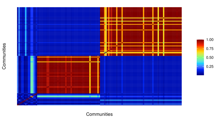
(a) Similarity matrix at depth 1.

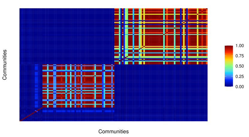
(b) Similarity matrix at depth 2.

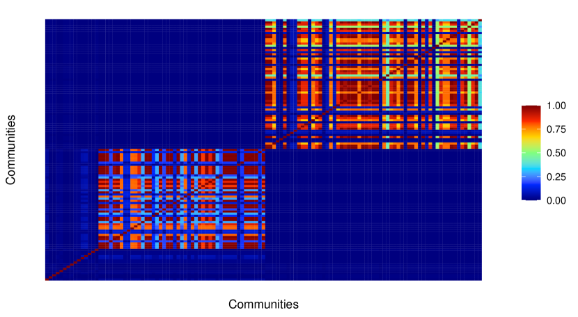
(c) Similarity matrix at depth 3.

Figure figure: Posterior similarity matrices at different depths for crime and communities data.

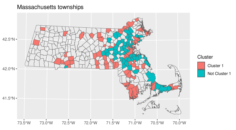
(a) Map plot of Massachusetts communities, colored membership of a depth 1 cluster.

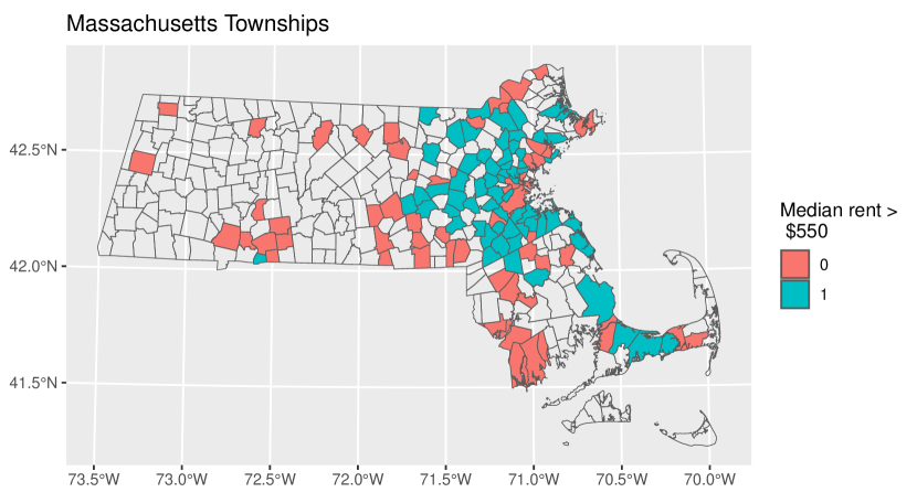
(b) Map plot of Massachusetts communities, colored by whether median rent is above threshold.

Figure figure: The communities in the largest cluster, red in panel (a), at depth $1$ of the estimated dendrogram roughly match with those with median rent above $\$550$ in panel (b).

section Discussion

Our work is motivated by improving computational efficiency of posterior inference for tree parameters. Expanding beyond the application to dendrograms, it is of interest to develop spanning tree-augmented models for more complex models, such as more elaborate discrete latent structure models (Zeng et al., 2023) or treed Gaussian process (Gramacy & Lee, 2008; Payne et al., 2024). For broader classes of tree models that may not admit a product-over-edges probability distribution, one may modify our random walk cover algorithm to form a computationally efficient proposal-generating distribution. Some related Metropolis-Hastings algorithms for sampling graph partitions have been recently studied by Autry et al. (2023). For a tree with unknown node size or structural dependence on a latent arrival process, such as diffusion trees (Neal, 2003) or Bayesian phylogenetic trees (Huelsenbeck & Ronquist, 2001), it is interesting to explore extending the fast-forwarding algorithm to bypass wasteful random walks on an infinite graph, or under time-varying transition probabilities.

Appendix 1

Proofs

Proof for Theorem 2

Proof .theorem.

Considering $(\hat{t}_{k+1}-\hat{t}_{k})$ as the inter-arrival time, we want to show that

$$\mathbb{E}(\hat{t}_{k+1}-\hat{t}_{k})\geq 1/\tilde{q},\qquad\tilde{q}=1+\min_{j\in U_{k}}\frac{\sum_{l\in U_{k}}w_{j,l}}{\sum_{l^{\prime}\in\bar{U}_{k}}w_{j,l^{\prime}}}.$$

Consider a sequence of independent Bernoulli events with success probabilities $p_{1},p_{2},\ldots$, with all $p_{i}\leq\tilde{q}$, and denote the index on the first success in this sequence by $T$. If $\mathbb{E}T<\infty$ then $\mathbb{E}T\geq 1/q$. Since $T\geq 0$, we know $\mathbb{E}T=\sum_{t=0}^{\infty}\text{Pr}(T>t)=\sum_{t=1}^{\infty}\prod_{i=1}^{t}(1-p_{i})\geq\sum_{t=1}^{\infty}\prod_{i=1}^{t}(1-\tilde{q})=1/\tilde{q}$. Adding over $\hat{t}=\sum_{k=1}^{m}(\hat{t}_{k+1}-\hat{t}_{k})$ with $\hat{t}_{1}=0$ yields the result.

Proof for Theorem 3

Proof .theorem.

We first state the Cheeger inequality for circulation graphs [Chung (2005), Theorem 3]. For a directed and weighted graph with non-negative weight matrix $W$, having $\sum_{l=1}^{m}w_{j,l}=\sum_{l=1}^{m}w_{l,j}$ for all $j$, the second smallest eigenvalue $\lambda_{2}(\mathcal{L})$ satisfies

$$\sqrt{\lambda_{2}(\mathcal{L})}\geq\min_{U:1\leq|U|\leq m-1}\frac{\sum_{j\in U,l\in\bar{U}}w_{j,l}}{\min(\sum_{j\in U}d_{j},\sum_{j\in\bar{U}}d_{j})}.$$

Letting $U=\cap_{\tilde{t}\leq t}X_{\tilde{t}}$, $|U|\leq m-1$, the probability of exiting $U$ at time $t+1$ is

$$\text{Pr}(x_{t+1}\in\bar{U}\mid x_{t}\in U) =\sum_{j\in U}\bigg{\{}\frac{\sum_{l\in\bar{U}}w_{j,l}}{d_{j}}S_{t}(j)\bigg{\}}.$$

Using $\tilde{e}_{j}=\sum_{l\in\bar{U}}w_{j,l}$, we obtain

$$\bigg{[}\sum_{j\in U}\bigg{\{}\frac{\tilde{e}_{j}}{d_{j}}S_{t}(j)\bigg{\}}\bigg{]}\sum_{j\in U}d_{j}=\sum_{j\in U}\bigg{\{}\tilde{e_{j}}S_{t}(j)\frac{\sum_{j^{\prime}\in U}d_{j^{\prime}}}{d_{j}}\bigg{\}}$$

$$\leq\sum_{j\in U}{\tilde{e}_{j}}\max_{j\in U}\bigg{\{}S_{t}(j)\frac{\sum_{j^{\prime}\in U}d_{j^{\prime}}}{d_{j}}\bigg{\}}\leq\Big{(}\sum_{j\in U}{\tilde{e}_{j}}\Big{)}\max_{j\in U\cup\bar{U}}\bigg{\{}S_{t}(j)\frac{\sum_{j^{\prime}\in U\cup\bar{U}}d_{j^{\prime}}}{d_{j}}\bigg{\}}.$$

After rearranging terms, we obtain:

$$\text{Pr}(x_{t+1}\in\bar{U}\mid x_{t}\in U)\leq\frac{\sum_{j\in U}\tilde{e}_{j}}{\sum_{j\in U}d_{j}}\max_{j\in U\cup\bar{U}}\bigg{\{}S_{t}(j)\frac{\sum_{j^{\prime}}d_{j^{\prime}}}{dj}\bigg{\}}$$

$$\leq\frac{\sum_{j\in U}\tilde{e}_{j}}{\min(\sum_{j\in U}d_{j},\sum_{j\in\bar{U}}d_{j})}\max_{j\in U\cup\bar{U}}\bigg{\{}S_{t}(j)\frac{\sum_{j^{\prime}}d_{j^{\prime}}}{d_{j}}\bigg{\}}$$

$$\leq\frac{\sum_{j\in U}\tilde{e}_{j}}{\min(\sum_{j\in U}d_{j},\sum_{j\in\bar{U}}d_{j})}\max_{j\in U\cup\bar{U}}\bigg{\{}S_{t}(j)\frac{\sum_{j^{\prime}}d_{j^{\prime}}}{d_{j}}\bigg{\}}.$$

Using $\pi_{j}=d_{j}/\sum_{j^{\prime}}d_{j^{\prime}}$ and taking the minimum over both sides, we have

$$\min_{U:|U|\leq m-1}\text{Pr}(x_{t+1}\in\bar{U}\mid x_{t}\in U)\leq\sqrt{\lambda_{2}(\mathcal{L})}\max_{j}S_{t}(j)/\pi_{j}.$$

Letting $U_{k^{*}}$ be the solution to the above inequality, by a similar argument in the proof of Theorem 2,

$$\mathbb{E}(\hat{t}_{k^{*}+1}-\hat{t}^{*}_{k})\geq\frac{1}{M\sqrt{\lambda_{2}(\mathcal{L})}}.$$

Adding the other $(m-2)$ steps, each with $\hat{t}_{k^{\prime}+1}-\hat{t}_{k^{\prime}}\geq 1$, leads to the result.

Proof for Theorem 4

Proof .theorem.

The Neumann series converges if the spectral radius $\lambda_{1}(P_{U,U})<1$ strictly. Since $P_{U,U}$ is a non-negative matrix, by Perron–-Frobenius theorem, $\lambda_{1}(P_{U,U})\leq\max_{i}\sum_{j}p_{i,j}\leq 1$.

Since $P_{U,U}$ is irreducible, by Perron–-Frobenius theorem, there exists a unique vector $P^{T}_{U,U}\phi_{*}=\lambda_{1}(P_{U,U})\phi_{*}$, with $\phi_{*}$ all positive and $1^{T}\phi_{*}=1$. We follow Chapter 8 of Meyer (2023), and let $Q$ be a non-negative matrix such that $P^{T}_{U,U}+Q$ has each column summable to 1, hence $1^{T}(P^{T}_{U,U}+Q)\phi\leq 1$ for any $\phi$ all positive and $1^{T}\phi=1$. Since there exists at least $\eta_{j}>0$, we know at least one $Q_{j,l}>0$.

If $\lambda_{1}(P_{U,U})=1$, we would have

$$1^{T}(P^{T}_{U,U}+Q)\phi_{*}=1^{T}\phi_{*}+1^{T}Q\phi_{*}>1,$$

which is a contradiction. Therefore, we know $\lambda_{1}(P_{U,U})<1$.

Supplementary Materials

.subsection Comparisons of number of iterations

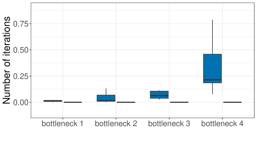
(a) Number of iterations to finish over different bottleneck rates $1/\sqrt{\lambda_{2}(\mathcal{L})}$.

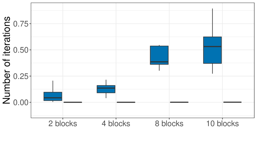
(b) Number of iterations to finish over different numbers of blocks (hence the numbers of bottlenecks).

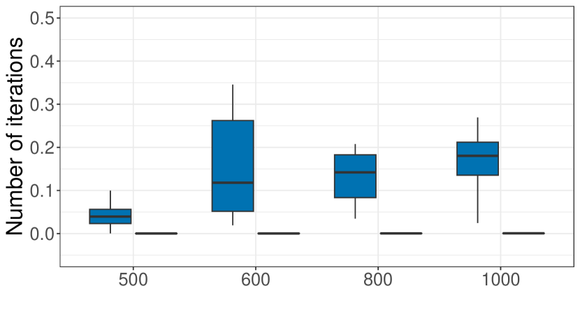
(c) Number of iterations to finish over different numbers of nodes.

Figure figure: Comparisons of number of iterations to finish between random walk cover (blue) and fast-forwarded cover (grey) algorithm.

.subsection Spanning tree-augmented dendrogram Gibbs sampler

The proposed Gibbs sampler iterates between the following sampling steps:

• Update the undirected version of the spanning tree $T$ from the full conditional $\Pi(T\mid-)$, which is a spanning tree distribution of product-over-edges form, using the fast-forwarded cover algorithm. Form a directed tree $\vec{T}$ from $T$ by assigning $0$ as the root, and having all edges pointed away from $0$;

• For $i=1,\ldots,n$, update $z_{i}$ from the full conditional $\Pi(z_{i}=k\mid-)$, a categorical distribution over $1,\cdots\tilde{m}$;

• Update $(\pi_{1},\cdots,\pi_{\tilde{m}})$ from the full conditional $\Pi(\pi_{1},\cdots,\pi_{\tilde{m}}\mid-)$, a Dirichlet distribution;

• Update the $\mu_{k}$’s and $\Sigma$ from the full conditional $\Pi(\mu_{2},\cdots,\mu_{\tilde{m}},\Sigma\mid-)$, which takes the form of a normal-inverse-Wishart distribution.

Recall that the root parameter $\mu_{1}$ is set at $0$. Once tree samples have been collected, pruning steps outlined in section section are performed to obtain the reduced dendrograms.

.subsection Details on plots on posterior similarity matrices and Massachusetts map

Posterior similarity matrices at depths $1,2,3$ were generated for $n=123$ Massachusetts communities available in the crimes and communities dataset. Each row/column in the matrix corresponds to a community. The $ij$th entry of the posterior similarity matrix at depth $R$ corresponds to the fraction of Gibbs sampler iterations for which the two communities share an ancestor node at depth $R$. The posterior similarity matrix was computed on samples $3501$ to $5000$ with thinning factor $10$. The depth $1$ posterior similarity matrix is then reordered according to the output of a spectral biclustering algorithm to reveal block-diagonal structures. The same ordering is applied to all 3 posterior similarity matrices at depths $1,2,3$. Maps data were obtained from the Massachusetts government website. The data from the crimes and communities dataset do not include all Massachusetts towns/cities. Counties that are missing from the dataset are set to transparent on the map.

.subsection Details for reversible-jump Markov chain Monte Carlo

We use $V_{\vec{T}}$ as the set of nodes in the dendrogram, and $V_{\vec{T}}^{C}=(1,\ldots,\tilde{m})\setminus V_{\vec{T}}$ as the other nodes not on the dendrogram. Further, we use $V^{\text{empty-leaf}}_{\vec{T}}$ to denote the node set $\{k\in V_{\vec{T}}:k\text{ has no children},n_{k}=0\}$.

We use the same full conditional distributions as in the main text to update $(\pi_{1},\ldots,\pi_{\tilde{m}})$, and those $\mu_{k}$ with $k\in V_{\vec{T}}$. When updating $z_{i}$, we use the same multinomial distribution, except with $\phi(y_{i};\mu_{k},\Sigma)$ replaced by zero density if $k\in V_{\vec{T}}^{C}$.

For updating the dendrogram, we use the proposals of birth and death steps in each iteration. We draw a binary $u\sim\text{Bern}(p_{0})$: if $u=1$, we use the birth proposal unless $|V_{\vec{T}}|=n$; if $u=0$, we use the death proposal unless $|V_{\vec{T}}|=1$. Therefore, we have the birth probability $p_{\text{birth}}(\vec{T})=p_{0}$ if $|V_{\vec{T}}|<n$, and $0$ otherwise; and the death probability $p_{\text{death}}(\vec{T})=1-p_{0}$ if $|V_{\vec{T}}|>1$, and $0$ otherwise. In our simulations, we set $p_{0}=0.1$.

• (Birth) Grow a new edge: draw $j$ uniformly from $V_{\vec{T}}$, find the smallest index $l$ from $V^{C}_{\vec{T}}$, draw $\mu_{l}\sim\mathcal{G}(\mu_{l}\mid\mu_{j})$, and attach $(j\to l)$ to $\vec{T}$ to form a proposed $\vec{T}^{*}$. Accept the $\vec{T}^{*}$ with probability

  $$\min\bigg{\{}1,\frac{0.01p_{\text{death}}(\vec{T}^{*})|V^{\text{empty-leaf}}_{\vec{T}^{*}}|^{-1}}{p_{\text{birth}}(\vec{T})|V_{\vec{T}}|^{-1}}\bigg{\}}.$$ (equation)

• (Death) Prune an empty leaf node: draw $j$ uniformly from $V^{\text{empty-leaf}}_{\vec{T}}$, remove $j$ from $\vec{T}$ to form a proposed $T^{*}$. Accept the $\vec{T}^{*}$ with probability

  $$\min\bigg{\{}1,\frac{p_{\text{birth}}(\vec{T}^{*})|V_{\vec{T}^{*}}|^{-1}}{0.01p_{\text{death}}(\vec{T})|V^{\text{empty-leaf}}_{\vec{T}}|^{-1}}\bigg{\}},$$ (equation)

  provided that the current $\vec{T}$ has $|V^{\text{empty-leaf}}_{\vec{T}}|>0$. If $|V^{\text{empty-leaf}}_{\vec{T}}|=0$ skip the step.

In the above, the Metropolis-Hastings acceptance ratio has a simple form because in the birth step, the product of the likelihood at ${\vec{T}}$ and the proposal density for $\mu_{l}$ satisfy $L(y;(\mu_{j})_{j\in V_{\vec{T}}},\vec{T},\cdot)\mathcal{G}(\mu_{l}\mid\mu_{j})=L(y;(\mu_{j})_{j\in V_{\vec{T}^{*}}},\vec{T}^{*},\cdot)$, hence canceling out the likelihood at the proposed state; and the transform $\{(\mu_{j})_{j\in V_{\vec{T}}},\mu_{l}\}\leftrightarrow(\mu_{j})_{j\in V_{\vec{T}^{*}}}$ is one-to-one and has Jacobian determinant 1.

.subsection Modifications for Forest Models

\begin{overpic}[width=433.62pt]{art/gibbs/gibbs_depth_trace.pdf} \put(45.0,-1.0){\scriptsize Iteration} \end{overpic}

(a) Trace plot of depth.

\begin{overpic}[width=433.62pt]{art/gibbs/gibbs_depth_dens.pdf} \put(50.0,-1.0){\scriptsize Depth} \end{overpic}

(b) Bar plot of depth.

\begin{overpic}[width=433.62pt]{art/gibbs/gibbs_depth_acf.pdf} \put(50.0,-1.0){\scriptsize Lag} \end{overpic}

(c) Autocorrelation plot of depth.

Figure figure: Trace, bar and autocorrelation plots for the depth of the tree samples from the Gibbs sampler.

\begin{overpic}[width=433.62pt]{art/rjmcmc/rjmcmc_depth_trace.pdf} \put(45.0,-1.0){\scriptsize Iteration} \end{overpic}

(a) Trace plot of depth.

\begin{overpic}[width=433.62pt]{art/rjmcmc/rjmcmc_depth_dens.pdf} \put(50.0,-1.0){\scriptsize Depth} \end{overpic}

(b) Bar plot of depth.

\begin{overpic}[width=433.62pt]{art/rjmcmc/rjmcmc_depth_acf.pdf} \put(50.0,-1.0){\scriptsize Lag} \end{overpic}

(c) Autocorrelation plot of depth.

Figure figure: Trace, bar and autocorrelation plots for the depth of the tree samples from the reversible-jump Markov chain Monte Carlo sampler.

We can view $\cup_{k=1}^{K}\vec{T}_{k}$ that arise from a forest model (equation) as a spanning tree in the following manner. One can consider an auxiliary graph $G$ with $(1,\ldots,n+1)$ nodes, with $q_{j,l}=\mathcal{H}(\mu_{l}\mid\mu_{j})$ for $j,l\leq n$ and $q_{n+1,r_{k}}=\mathcal{F}(y_{r_{k}})$ for $r_{k}\leq n$. Then, first specify $\vec{\mathcal{T}}$ as a large spanning tree rooted at $(n+1)$ and then cut all $K$ edges adjacent to $(n+1)$ to obtain $\cup_{k=1}^{K}\vec{T}_{k}$. Our algorithm can be therefore be applied to the proposed class of forest models.

.subsection Normalized Laplacian

For any non-negative weight matrix $W$, define the normalized Laplacian (Chung, 1997) as

$$\mathcal{L}=I-\frac{1}{2}\big{\{}\Phi^{1/2}(D^{-1}W)\Phi^{-1/2}+\Phi^{-1/2}(W^{T}D^{-1})\Phi^{1/2}\big{\}},$$

where $\Phi=\text{diag}(\pi_{j})_{j=1}^{m}$ and $D=\text{diag}(d_{j})_{j=1}^{m}$. Since $\sum_{l=1}^{m}\pi_{j}(w_{j,l}/d_{j})=\sum_{k=1}^{m}\pi_{k}(w_{k,j}/d_{k})$ holds for $\pi_{j}=d_{j}/(\sum_{k=1}^{m}d_{k}),$ the normalized Laplacian reduces to

$$\mathcal{L}=I-D^{-1/2}\frac{W+W^{T}}{2}D^{-1/2}.$$

The above form further reduces to $\mathcal{L}=I-D^{-1/2}WD^{-1/2}$ if $W=W^{T}$.

References

- Aldous (1990) Aldous, D. J. (1990). The random walk construction of uniform spanning trees and uniform labelled trees. SIAM Journal on Discrete Mathematics 3, 450–465.
- Autry et al. (2023) Autry, E., Carter, D., Herschlag, G. J., Hunter, Z. & Mattingly, J. C. (2023). Metropolized forest recombination for Monte Carlo sampling of graph partitions. SIAM Journal on Applied Mathematics 83, 1366–1391.
- Broder (1989) Broder, A. Z. (1989). Generating random spanning trees. In 30th Annual Symposium on Foundations of Computer Science.
- Broder & Karlin (1989) Broder, A. Z. & Karlin, A. R. (1989). Bounds on the cover time. Journal of Theoretical Probability 2, 101–120.
- Castillo & Ročková (2021) Castillo, I. & Ročková, V. (2021). Uncertainty quantification for Bayesian CART. The Annals of Statistics 49, 3482–3509.
- Chipman et al. (1998) Chipman, H. A., George, E. I. & McCulloch, R. E. (1998). Bayesian CART model search. Journal of the American Statistical Association 93, 935–948.
- Chipman et al. (2010) Chipman, H. A., George, E. I. & McCulloch, R. E. (2010). BART: Bayesian additive regression trees. The Annals of Applied Statistics 4, 266 – 298.
- Chung (1997) Chung, F. (1997). Spectral Graph Theory, vol. 92. American Mathematical Soc.
- Chung (2005) Chung, F. (2005). Laplacians and the Cheeger inequality for directed graphs. Annals of Combinatorics 9, 1–19.
- Denison et al. (1998) Denison, D. G., Mallick, B. K. & Smith, A. F. (1998). A Bayesian CART algorithm. Biometrika 85, 363–377.
- Duan & Dunson (2023) Duan, L. L. & Dunson, D. B. (2023). Bayesian spanning tree: estimating the backbone of the dependence graph. The Journal of Machine Learning Research 24, 1–44.
- Duan & Roy (2023) Duan, L. L. & Roy, A. (2023). Spectral clustering, Bayesian spanning forest, and forest process. Journal of the American Statistical Association , 1–24.
- Elidan & Gould (2008) Elidan, G. & Gould, S. (2008). Learning bounded treewidth Bayesian networks. Advances in Neural Information Processing Systems 21.
- Fredes & Marckert (2023) Fredes, L. & Marckert, J.-F. (2023). A combinatorial proof of Aldous–Broder theorem for general Markov chains. Random Structures & Algorithms 62, 430–449.
- Fritsch & Ickstadt (2009) Fritsch, A. & Ickstadt, K. (2009). Improved criteria for clustering based on the posterior similarity matrix. Bayesian Analysis 4, 367 – 391.
- Gower & Ross (1969) Gower, J. C. & Ross, G. J. (1969). Minimum spanning trees and single linkage cluster analysis. Journal of the Royal Statistical Society: Series C (Applied Statistics) 18, 54–64.
- Gramacy & Lee (2008) Gramacy, R. B. & Lee, H. K. H. (2008). Bayesian treed Gaussian process models with an application to computer modeling. Journal of the American Statistical Association 103, 1119–1130.
- Heard et al. (2006) Heard, N. A., Holmes, C. C. & Stephens, D. A. (2006). A quantitative study of gene regulation involved in the immune response of anopheline mosquitoes: an application of Bayesian hierarchical clustering of curves. Journal of the American Statistical Association 101, 18–29.
- Heller & Ghahramani (2005) Heller, K. A. & Ghahramani, Z. (2005). Bayesian hierarchical clustering. In Proceedings of the 22nd International Conference on Machine Learning.
- Huelsenbeck & Ronquist (2001) Huelsenbeck, J. P. & Ronquist, F. (2001). MRBAYES: Bayesian inference of phylogenetic trees. Bioinformatics 17, 754–755.
- Kruskal (1956) Kruskal, J. B. (1956). On the shortest spanning subtree of a graph and the traveling salesman problem. Proceedings of the American Mathematical Society 7, 48–50.
- Lauritzen (2011) Lauritzen, S. L. (2011). Elements of graphical models. Lectures From the XXXVIth International Probability Summer School in St-Flour, France. .
- Levin & Peres (2017) Levin, D. A. & Peres, Y. (2017). Markov Chains and Mixing Times, vol. 107. American Mathematical Soc.
- Linero & Yang (2018) Linero, A. R. & Yang, Y. (2018). Bayesian regression tree ensembles that adapt to smoothness and sparsity. Journal of the Royal Statistical Society Series B: Statistical Methodology 80, 1087–1110.
- Lovász & Winkler (1993) Lovász, L. & Winkler, P. (1993). A note on the last new vertex visited by a random walk. Journal of Graph Theory 17, 593–596.
- Luo et al. (2021) Luo, Z. T., Sang, H. & Mallick, B. (2021). A Bayesian contiguous partitioning method for learning clustered latent variables. The Journal of Machine Learning Research 22, 1748–1799.
- Luo et al. (2023) Luo, Z. T., Sang, H. & Mallick, B. (2023). A nonstationary soft partitioned Gaussian process model via random spanning trees. Journal of the American Statistical Association 0, 1–12.
- Matthews (1988) Matthews, P. (1988). Covering problems for Markov chains. The Annals of Probability 16, 1215–1228.
- Meilă & Jaakkola (2006) Meilă, M. & Jaakkola, T. (2006). Tractable Bayesian learning of tree belief networks. Statistics and Computing 16, 77–92.
- Meilă & Jordan (2000) Meilă, M. & Jordan, M. I. (2000). Learning with mixtures of trees. Journal of Machine Learning Research 1, 1–48.
- Meyer (2023) Meyer, C. D. (2023). Matrix Analysis and Applied Linear Algebra, vol. 188. SIAM.
- Neal (2003) Neal, R. M. (2003). Density modeling and clustering using Dirichlet diffusion trees. Bayesian Statistics 7, 619–629.
- Payne et al. (2024) Payne, R. D., Guha, N. & Mallick, B. K. (2024). A Bayesian survival treed hazards model using latent Gaussian processes. Biometrics 80, ujad009.
- Prim (1957) Prim, R. C. (1957). Shortest connection networks and some generalizations. The Bell System Technical Journal 36, 1389–1401.
- Saad (2003) Saad, Y. (2003). Iterative Methods for Sparse Linear Systems. SIAM.
- Suchard et al. (2001) Suchard, M. A., Weiss, R. E. & Sinsheimer, J. S. (2001). Bayesian selection of continuous-time Markov chain evolutionary models. Molecular Biology and Evolution 18, 1001–1013.
- Teixeira et al. (2019) Teixeira, L. V., Assunção, R. M. & Loschi, R. H. (2019). Bayesian space-time partitioning by sampling and pruning spanning trees. The Journal of Machine Learning Research 20, 1.
- Van Havre et al. (2015) Van Havre, Z., White, N., Rousseau, J. & Mengersen, K. (2015). Overfitting bayesian mixture models with an unknown number of components. PloS One 10, e0131739.
- Wilson (1996) Wilson, D. B. (1996). Generating random spanning trees more quickly than the cover time. In Proceedings of the Twenty-Eighth Annual ACM Symposium on Theory of Computing.
- Wu et al. (2007) Wu, Y., Tjelmeland, H. & West, M. (2007). Bayesian CART: prior specification and posterior simulation. Journal of Computational and Graphical Statistics 16, 44–66.
- Zeng et al. (2023) Zeng, Z., Gu, Y. & Xu, G. (2023). A tensor-EM method for large-scale latent class analysis with binary responses. Psychometrika 88, 580–612.