Loss Jump During Loss Switch in Solving PDEs with Neural Networks
Zhiwei Wang
Institute of Natural Sciences, School of Mathematical Sciences
Shanghai Jiao Tong University
Shanghai 200240, P.R. China
victorywzw@sjtu.edu.cn &Lulu Zhang
Institute of Natural Sciences, School of Mathematical Sciences
Shanghai Jiao Tong University
Shanghai 200240, P.R. China
zhangl9661@sjtu.edu.cn &Zhongwang Zhang
Institute of Natural Sciences, School of Mathematical Sciences
Shanghai Jiao Tong University
Shanghai 200240, P.R. China
0123zzw666@sjtu.edu.cn &Zhi-Qin John Xu
Institute of Natural Sciences, School of Mathematical Sciences
Shanghai Jiao Tong University
Shanghai 200240, P.R. China
xuzhiqin@sjtu.edu.cn
Abstract
Using neural networks to solve partial differential equations (PDEs) is gaining popularity as an alternative approach in the scientific computing community. Neural networks can integrate different types of information into the loss function. These include observation data, governing equations, and variational forms, etc. These loss functions can be broadly categorized into two types: observation data loss directly constrains and measures the model output, while other loss functions indirectly model the performance of the network, which can be classified as model loss. However, this alternative approach lacks a thorough understanding of its underlying mechanisms, including theoretical foundations and rigorous characterization of various phenomena. This work focuses on investigating how different loss functions impact the training of neural networks for solving PDEs. We discover a stable loss-jump phenomenon: when switching the loss function from the data loss to the model loss, which includes different orders of derivative information, the neural network solution significantly deviates from the exact solution immediately. Further experiments reveal that this phenomenon arises from the different frequency preferences of neural networks under different loss functions. We theoretically analyze the frequency preference of neural networks under model loss. This loss-jump phenomenon provides a valuable perspective for examining the underlying mechanisms of neural networks in solving PDEs.
Keywords loss jump, frequency bias, neural network, loss switch.
1 Introduction
The use of neural networks for solving partial differential equations (PDEs) has emerged as a promising alternative to traditional numerical methods in the scientific computing community. By incorporating various types of information into the loss function, such as observation data, governing equations, and variational forms, neural networks offer a flexible and powerful framework for approximating the solution of PDEs. These loss functions can be broadly classified into two categories: data loss, which directly constrains and measures the model output using observation data, and model loss, which indirectly models the performance of the network using equations and variational forms.
Despite the growing interest in this approach, a comprehensive understanding of the underlying mechanisms governing the behavior of neural networks in solving PDEs is still lacking. While several works have explored the capabilities and limitations of physics-informed learning [1, 2, 3, 4, 5] and the challenges in training physics-informed neural networks (PINNs) [1, 6], the impact of different loss functions on the training dynamics and convergence properties of neural networks remains an open question.
Recent studies have shown that the derivatives of the target functions in the loss function play a crucial role in the convergence of frequencies [1, 7, 8]. A key observation is that neural networks often exhibit a frequency principle, learning from low to high frequencies [1, 9, 10, 8]. This phenomenon has inspired a series of theoretical works aimed at understanding the convergence properties of neural networks [11, 12, 13, 14, 15].
Moreover, the development of deep learning theory and algorithms has greatly benefited from the accurate description of stable phenomena. For instance, it has been observed that heavily over-parameterized neural networks usually do not overfit [16, 17], neurons in the same layer tend to condense in the same direction [18, 19, 20], and stochastic gradient descent or dropout tends to find flat minima [21, 22, 23, 24, 25, 20]. Additionally, a series of multiscale neural networks have been developed for solving differential equations [26, 27, 28, 29, 30, 31] and fitting functions [32, 33].
Motivated by these findings, we aim to investigate the impact of different loss functions on the training dynamics and convergence properties of neural networks for solving PDEs. We focus on the interplay between data loss and model loss, which incorporate different orders of derivative information. We discover a stable loss-jump phenomenon: when switching the loss function from the data loss to the model loss, which includes different orders of derivative information, the neural network solution significantly deviates from the exact solution immediately.
In this work, we analyze the training process and the dynamics induced by different loss functions from a frequency-space perspective. We identify a multi-stage descent phenomenon, where the neural network’s ability to constrain low-frequency information is weak when using model loss functions. Furthermore, we model the training process of two-layer neural networks with two-order derivative loss and quantitatively prove that within a certain frequency range, neural networks with high-order derivative loss functions are more inclined to fit high-frequency information in the target function.
The insights gained from this study shed light on the complex interplay between loss functions, frequency preference, and convergence properties of neural networks in solving PDEs. By understanding these mechanisms, we aim to contribute to the development of more robust and efficient neural network-based PDE solvers and to advance the theoretical foundations of this rapidly evolving field.
2 Fitting Target Function with Different Loss Functions
Given an objective function , an appropriate loss function can be selected based on the available data to train a neural network that approximates the target function.
2.1 Data loss
Assuming a set of observation points and corresponding values , the mean squared error between the target function and the neural network output can be used as a loss function to train the network. This data loss is represented as
(1)
The data loss serves not only as a loss function for supervised learning but also as a direct measure of the distance between the model’s output and the true target function. Consequently, it is the most important metric for evaluating the performance of the algorithm. By minimizing the data loss, the optimal set of parameters is sought, enabling the neural network to closely approximate the target function .
2.2 Model loss
Model loss refers to the use of the governing equations of the target function as a supervised learning metric. By calculating the mean squared loss between the model’s predictions and the target function’s governing equations, the model loss function is obtained. The governing equations can take various forms, such as combinations of multi-order derivatives, PDE control equations, or variational formulations. Here are a few examples:
If the first-order derivatives of the function are available at several observation points, they can be used in conjunction with boundary and initial conditions to construct a loss function for training the neural network. Similarly, higher-order derivative information can also be incorporated into the loss function. Such a model loss can be represented as
(2)
where is the number of sampled -order derivative values of the objective function, and is the weight assigned to the corresponding loss term.
If the governing equation of the objective function is known, for example, if the function satisfies a PDE of the form
(3)
where denotes the spatial domain, is the time interval, is the exact solution, is the source term, and and are the initial and boundary conditions, respectively, the governing equation can be directly incorporated into the loss function. Specifically, the model loss can include the residual of the governing equation, initial value loss, boundary value loss, and optional supervised learning point loss:
(4)
where , , , and are the numbers of collocation points, training points sampled from the initial condition, training points on the boundary, and supervised learning points, respectively. , , , and are the corresponding weight hyperparameters used to balance the contributions of each loss term. It should be noted that the supervised learning point loss is not always necessary, as in most cases, the initial and boundary conditions along with the PDE form are sufficient to determine the solution.
Another approach is to use the variational form of the governing function as the loss function, which is known as the deep Ritz method. Suppose the variational form satisfied by is
(5)
Then the loss function can be designed as
(6)
Model loss provides a variety of choices for training neural networks and, when used appropriately, can accelerate convergence. However, it cannot directly measure the gap between the model’s output and the target function. In some cases, even when the model loss is small, the model’s error can be extremely large. For example, in the interval , if is trained using the first-order derivative, where is sufficiently small, the model loss is when the model output is 0, but the data loss is . Therefore, model loss serves as an indirect evaluation metric rather than a direct one.
3 Rapid Increase in Error When Switching Loss
In this work, we discover a loss-jump phenomenon: when switching the loss function from low-order to high-order derivatives, such as switching from data loss to model loss, the neural network solution significantly deviates from the exact solution immediately.
To illustrate this phenomenon, we begin with a simple Poisson problem:
(7)
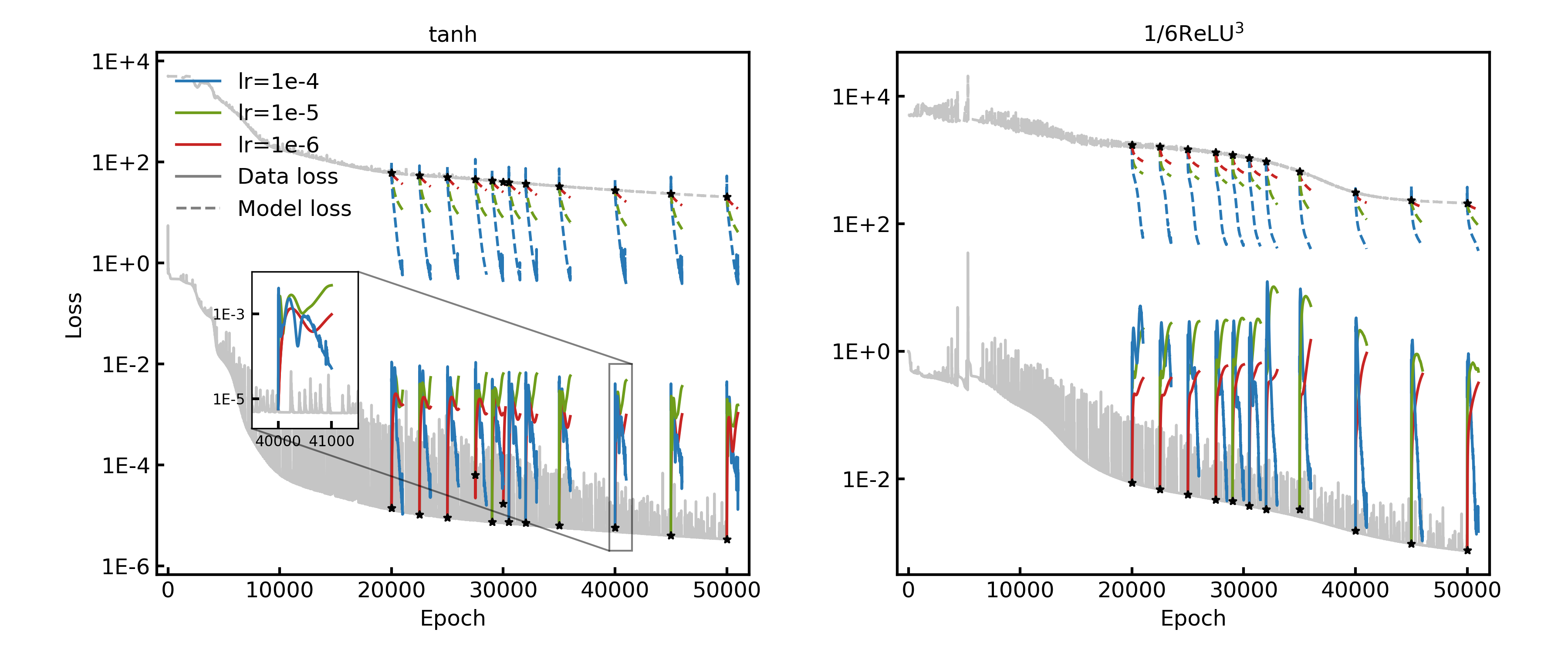
The exact solution to this problem is . We selected 5120 equidistant points as training data and employed a neural network with 3 hidden layers, each containing 320 neurons. The commonly used and cubic () activation functions were utilized, along with the Adam optimizer [34]. The data loss was trained for 100,000 epochs, and the model loss was introduced at different epochs to observe changes in both data and model losses. The model loss weights were set to , indicating that no additional supervised data points were used for model loss training. During pre-training, the learning rate was set to 1e-3, decaying to 92% of its original value every 1000 epochs. Different learning rates were employed after switching the loss function. As shown in Fig. 1, the results demonstrate that the increase in data loss after switching the loss function is consistent across different learning rates, indicating that this phenomenon is not caused by an excessively high learning rate.
Figure 1: Training process under different learning rate with tanh (left) and ReLU (right) activation function. The gray line indicates pre-training using the data loss function. The asterisk points the error when switching loss. The colored lines are different learning rates used.
The same experimental phenomenon can also be observed in other PDE equations. We examine several types of equations, including the Burgers equation, heat equation, diffusion equation, and wave equation.
The results are listed below. The neural network structure used is a fully connected network with 5 hidden layers, each containing 40 neurons. The activation function is employed, and the network is initialized using Glorot normal initialization [35]. The Adam optimizer is used for training. The first 50,000 epochs utilize model loss, with a learning rate of 1e-3 that decays to 92% of its original value every 1000 epochs. Both the training and test sets are Cartesian products of 500 equidistant space grid points and 11 equidistant time grid points. After switching to the model loss function, training continues for an additional 50,000 epochs. At each epoch, Monte Carlo sampling is used to select 8192 points within the region as the training dataset. The learning rate after switching the loss function is 1e-5 for the Burgers problem and 1e-4 for the others, decaying to 95% of its original value every 1000 epochs. Additionally, 100 points are selected at both the boundary and initial area for supervised learning. The test set remains the previously defined 5500 equidistant grid points. The weights for each component of the model loss are set to .
3.1 Burgers equation
The Burgers equation, proposed by Dutch mathematician Johannes Martinus Burgers in 1948, is often used to study fluid mechanics, turbulence, and shock waves. The equation captures the key physical processes of fluid motion, including nonlinear convective effects and viscous dissipation. It serves as a simple yet important model for understanding and studying complex fluid problems. The Burgers equation has the following form:
(8)
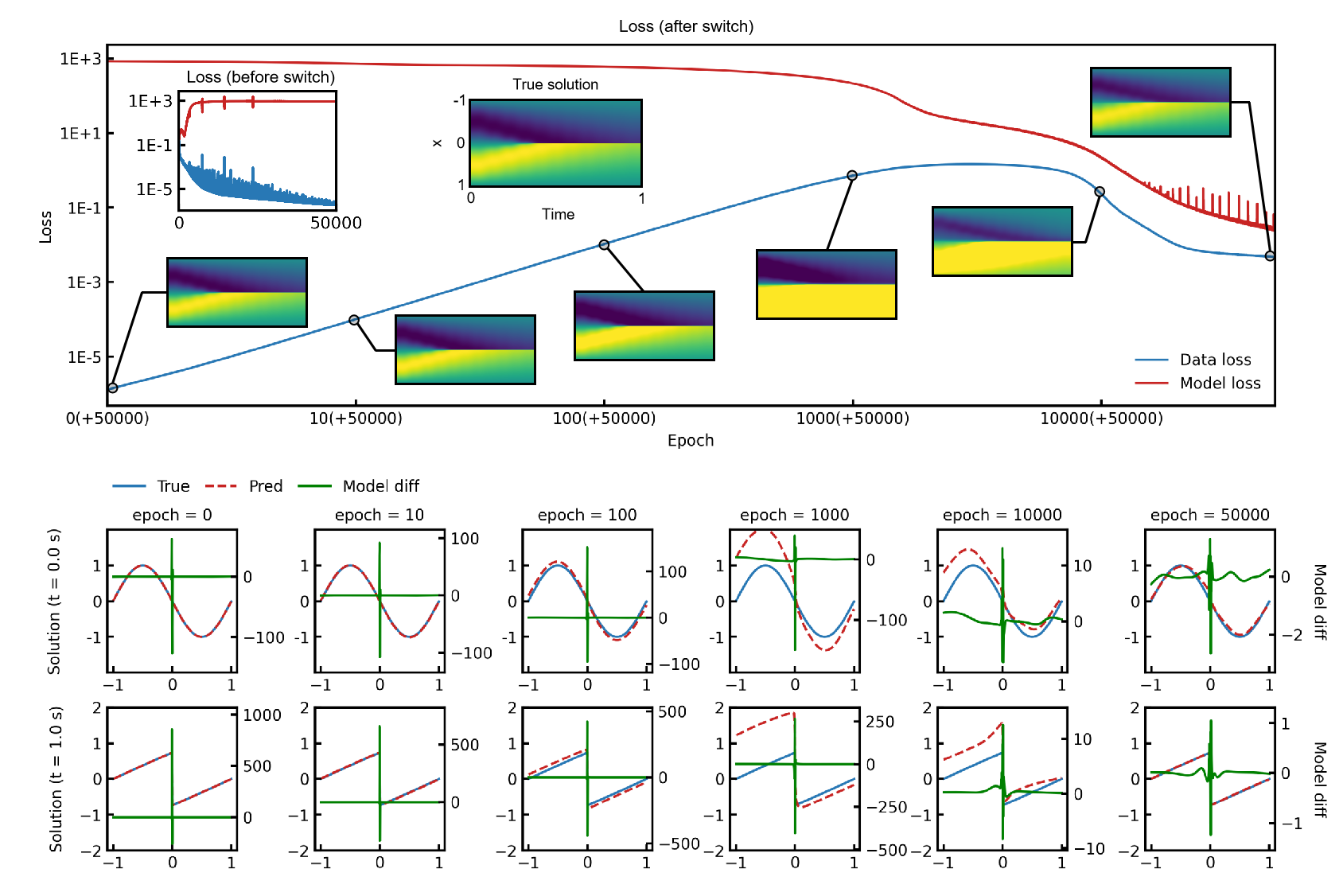
Figure 2: Burgers equation training process. The second and third rows are the changes of the network prediction value with the training process at time and time respectively after switching the loss.
Fig. 2 shows the results after switching to model loss following 50,000 epochs of data loss training. It can be observed that the predictions initially deviate as a whole and then converge to another minimum point.
3.2 Heat equation
The heat equation is a differential equation that describes heat conduction and diffusion. Here, we consider a classic example of the equation, which describes a purely conductive process without a heat source, following the assumption of local thermodynamic equilibrium:
(9)
And the analytical solution is .
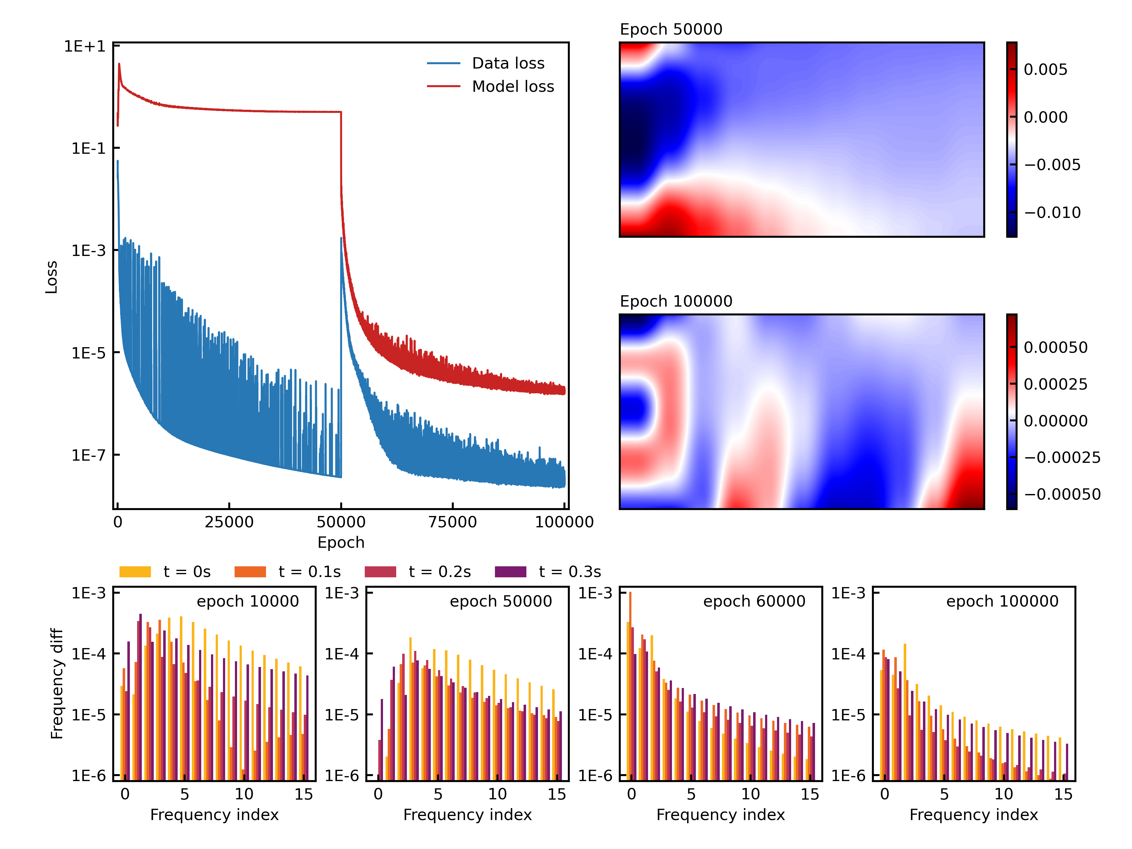
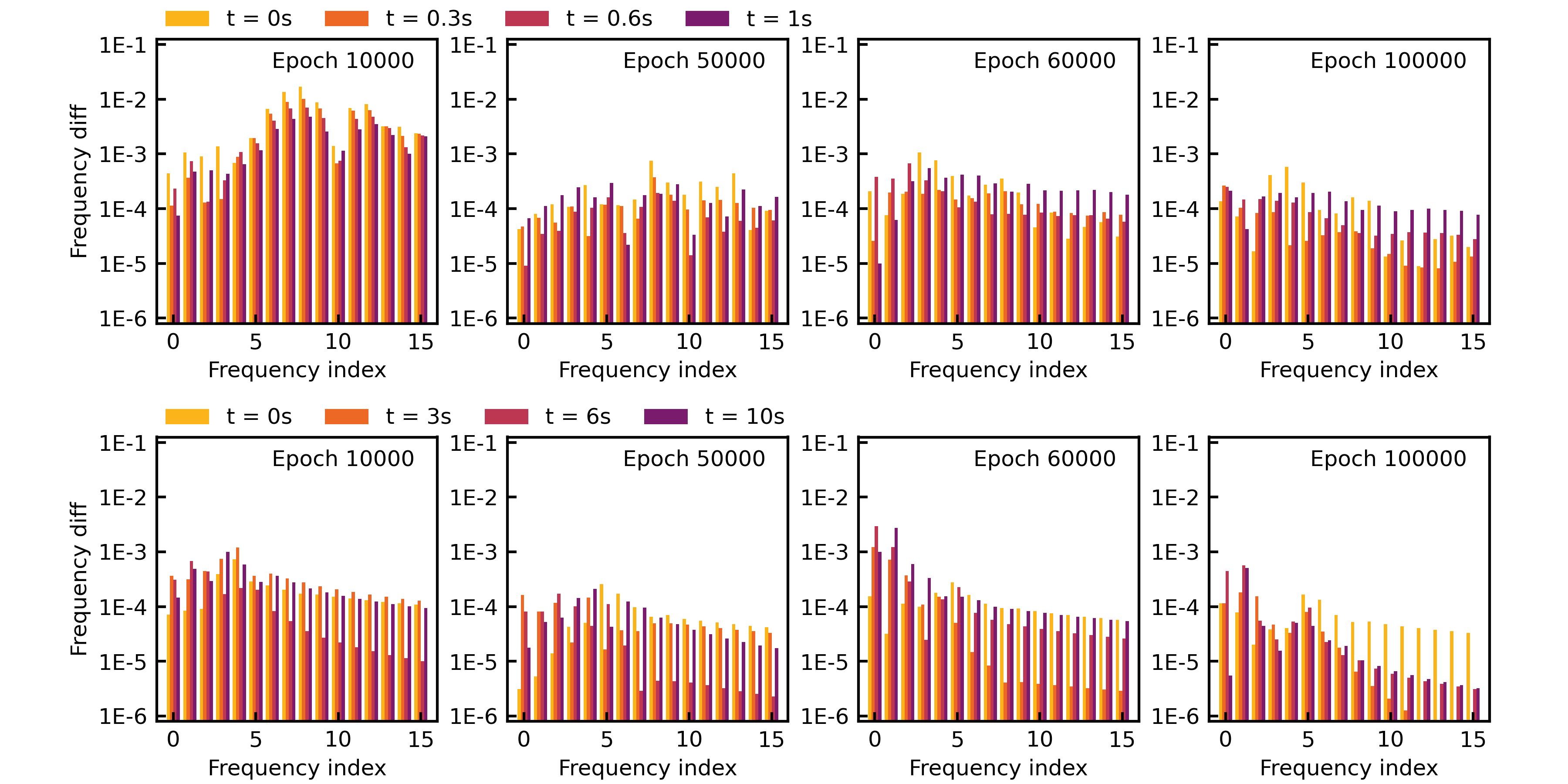
Figure 3: Heat equation training process. Upper left: data loss and model loss as the training progresses. Upper right: error heatmaps at 50,000 and 100,000 epochs. Bottom: Frequency error at different training epochs. The 4 sub-figures are the results from different training stage.
From the loss plot in the upper left corner of Fig.3, we can see that when switching to model loss after 50,000 epochs, the data loss rises sharply, indicating that the solution has jumped out of the local optimum. It is important to note that the model loss drops after switching, suggesting that this phenomenon is not caused by the shock of an excessively large learning rate. In fact, the learning rate of 1e-4 used in this experiment is much smaller than the learning rates typically used in physics-informed neural networks (PINNs). The two error heatmaps on the right illustrate that the minimum points obtained after switching the loss function differ from the original ones. We believe this may be due to the fact that the dynamical behaviors induced by the two loss functions exhibit different frequency preferences. The bottom row of Fig.3 shows the variation of frequency error at different training stages and time slices. In the first 50,000 epochs of training, it can be clearly seen that low-frequency information is fitted first. However, when the loss function is switched, the error shows a decreasing trend with frequency. This may be the main reason for the sudden increase in errors.
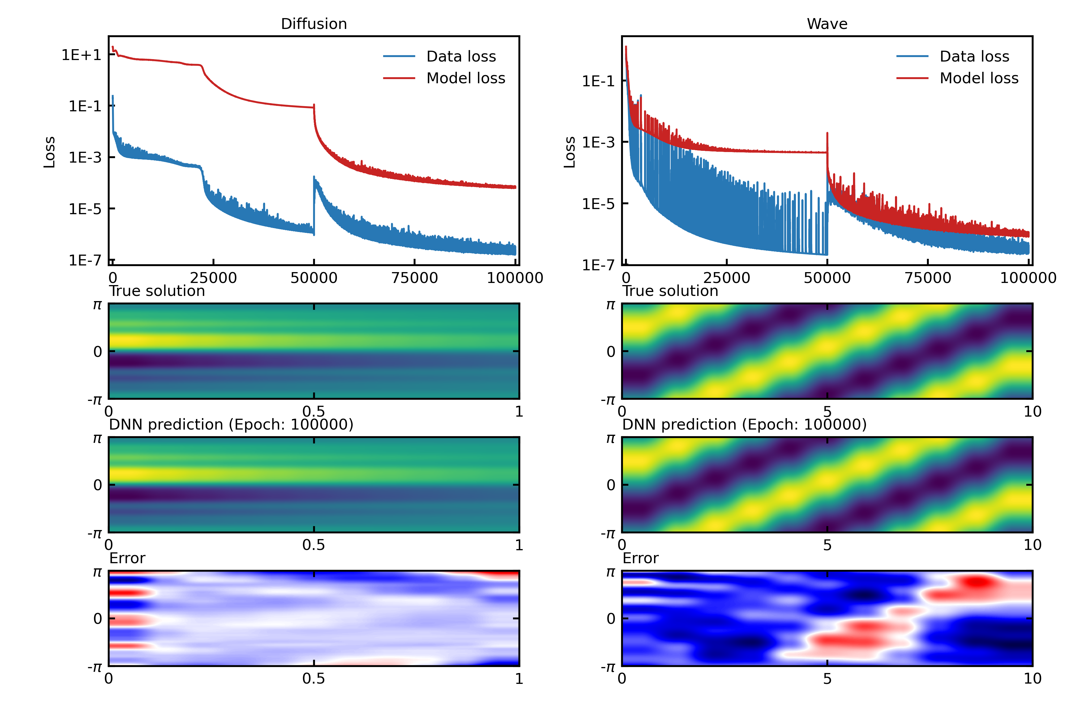
Figure 4: Diffusion equation (left) and wave equation (right) training process. Top: data loss and model loss as the training progresses. Middle: Heatmap of the analytical solution and the DNN-predicted solution. Bottom: Absolute error between analytical solution and DNN prediction.
3.3 Diffusion equation and wave equation
We also tested the diffusion equation and the wave equation and obtained similar results.
For the diffusion equation, we fabricated an analytical solution with decreasing frequency magnitudes. The PDE formulation of the diffusion equation is defined as:
(10)
The exact solution is .
For the wave equation, we used an analytical solution with only a single frequency. The wave equation is defined as:
(11)
The exact solution is .
Figure 5: Frequency error of diffusion equation (top) and wave equation (bottom).
From the frequency diagram, because the frequency amplitude of the function used for the diffusion equation decreases with frequency, the error at each frequency does not exhibit a significant decrease. However, it can still be observed that the fitting preference of the neural network for each frequency has changed before and after switching the loss function.
4 Multi-stage Descent Phenomenon
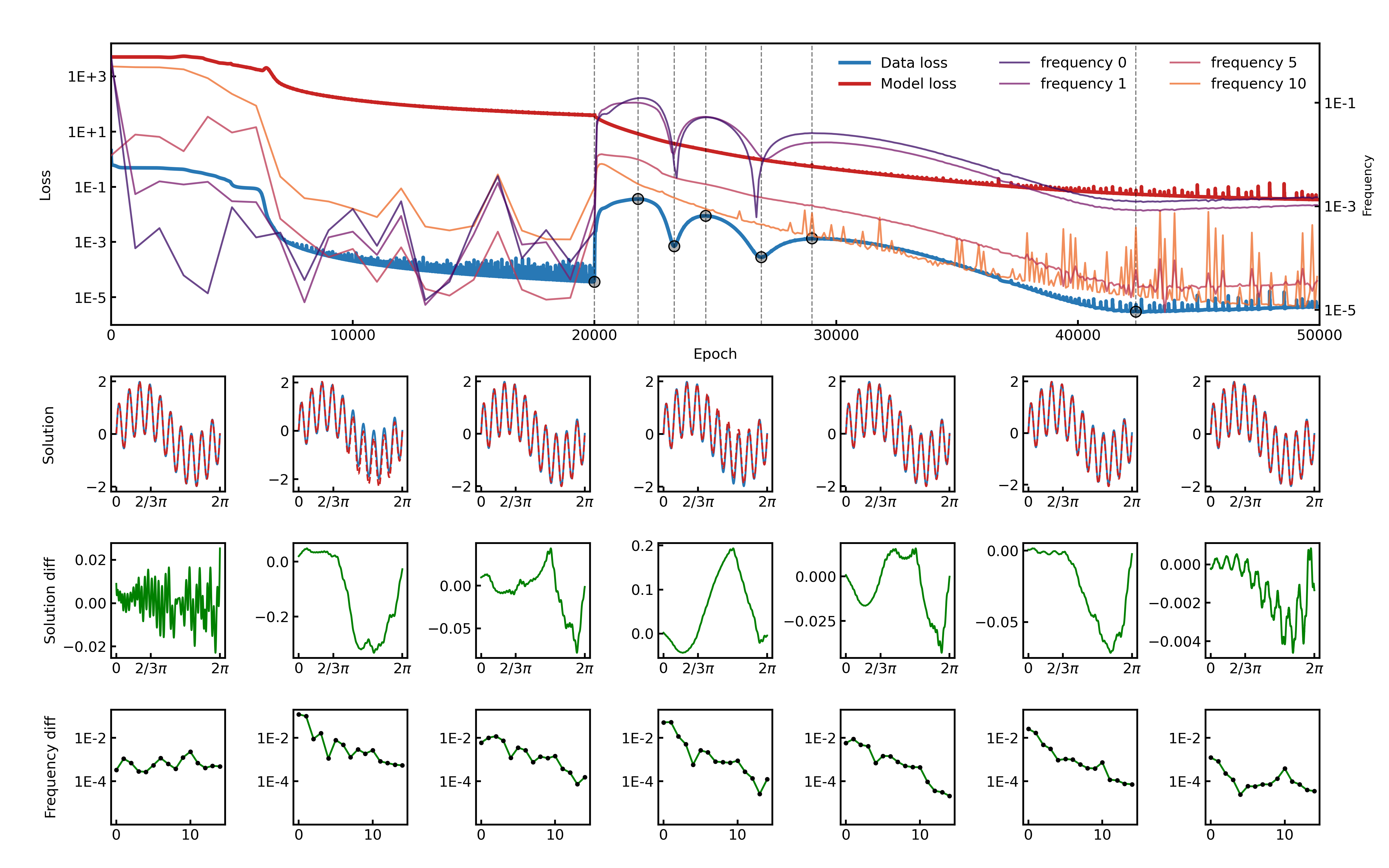
Figure 6: Multi-stage descent. We consider Eq. 7 and use a fully connected network with 2 layers of 40 neurons in each layer for training. First, the data loss function is used to train for 20,000 epochs, then switched to the model loss function. An additional supervised learning point is added at . The weights of each part in the model loss are . In the epoch-loss curve (top), we mark the 7 maximum or minimum points of the data loss curve. The 7 subgraphs in each subsequent row correspond to the states at these 7 points. The second row shows the predicted values of the neural network (red dotted line) and the exact solution (blue solid line). The third row is the curve of . The fourth row is the Fourier transform of .
We further observe the subsequent training process of the neural network for Equation 7 after switching to model loss. The difference from the previous experiment is that here we add a supervised learning point at . In Fig. 6, we plot the training error for 80,000 epochs after switching to model loss at 20,000 epochs and the prediction errors of the neural network at different stages. Since we previously noticed that the error increase is always accompanied by an overall shift in the predicted values, we suspect that the low-frequency error cannot be well-constrained during model loss training. We plot the Fourier transform of the error in the last row of Fig. 6. We find that during the continuous decline of model loss, data loss exhibits a multi-stage descent. When training reaches a maximum value, the error is relatively smooth, and the Fourier transform shows that the error decreases with frequency, with the low-frequency error at a relatively large level. When reaching a minimum value point, the low-frequency error decreases. However, subsequent training causes the low-frequency error to change sign, returning to another maximum value. This phenomenon demonstrates that model loss makes it difficult to constrain the low-frequency error.
5 Frequency Bias for NN with model loss
Numerous studies have established that under the data loss setting, neural networks with common activation functions such as ReLU and tanh exhibit a frequency principle, fitting low frequencies first and then progressively capturing higher frequencies [1, 9, 10, 8]. This frequency principle has been considered crucial for understanding the good generalization properties of neural networks. However, in our model loss setting, we discover that the frequency preference of neural networks differs from that observed under the data loss setting. This difference in frequency preference provides an explanation for the sudden jump in data loss when switching from data loss to model loss during training.
To better understand the frequency preference during model loss training, we model the dynamic behavior of using model loss to train the Poisson problem. The one-dimensional Poisson problem can be described as:
(12)
where is the unknown function to be solved, is a given source term, and is the problem domain. The boundary conditions are not specified here, as they can be incorporated into the supervised learning points. Denoting and as the exact solution and the neural network approximation, respectively, the loss function can be simplified as:
(14)
where is a weight used to balance the two error terms, and are the sets of collocation points for the governing equation and the supervised learning points, respectively.
We consider a two-layer DNN structure and use the GD algorithm to train it. Thus the parameters follow the following dynamics:
(15)
For a 2-layer infinite-width neural network that conforms to the linear frequency principle, by defining and
where the Fourier transform operator is defined by
Here we define 5 functions to simplify the representation of neural network derivation,
(18)
(21)
we can prove the following theorem:
Theorem 1(Dynamics for NN with model loss).
The dynamics have the following expression in the frequency domain for all :
(22)
(23)
Where with empirical density and
(24)
(25)
For the activation function, we have
(28)
(31)
If we temporarily ignore all derivative terms, we can get
(32)
(33)
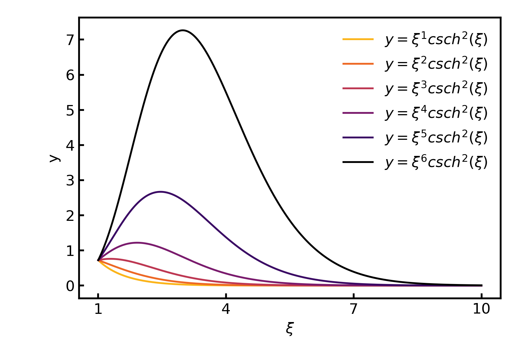
For one-dimensional problems, the convergence rate of frequency is governed by the function . As shown in Fig. 7, when the polynomial degree is large, increases with frequency within a certain range. Consequently, high frequencies exhibit faster convergence rates in this regime. However, once the frequency surpasses a certain threshold, rapidly decays with increasing frequency. From the perspective of a broader frequency spectrum, this behavior suggests that model loss tends to prioritize the learning of low and medium frequencies.
Figure 7: Values of for different polynomial degrees .
These findings highlight the complex interplay between frequency components and the convergence dynamics of neural networks under the model loss setting. The preferential learning of low and medium frequencies by model loss may have implications for the overall performance and generalization ability of the trained networks. Further research is needed to fully understand the impact of this frequency bias on the effectiveness of model loss-based training approaches for solving partial differential equations and other related problems.
6 Discussion
The loss jump phenomenon observed when switching from data loss to model loss highlights the complex interplay between loss functions, frequency bias, and convergence behavior in neural networks for solving partial differential equations. The sudden increase in data loss suggests that the solutions obtained using data loss may not provide a suitable starting point for model loss optimization, challenging the conventional wisdom of pre-training with data loss.
The multi-stage descent phenomenon suggests that model loss imposes weak constraints on low-frequency errors, which could have implications for the accuracy and reliability of the trained networks. Furthermore, our theoretical analysis reveals that model loss exhibits a frequency bias that differs from the well-established frequency principle observed in networks trained with data loss. Within a certain frequency range, high frequencies converge faster under model loss, while low and medium frequencies are prioritized when considering the entire spectrum. This difference in frequency preference provides a plausible explanation for the loss jump phenomenon.
Future research directions could include the development of adaptive training strategies, frequency-dependent weighting schemes, and regularization techniques to mitigate the impact of the loss jump and improve the performance of model loss-based approaches in scientific computing and engineering applications.
References
[1]
Zhi-Qin John Xu, Yaoyu Zhang, Tao Luo, Yanyang Xiao, and Zheng Ma.
Frequency principle: Fourier analysis sheds light on deep neural networks.
Communications in Computational Physics, 28(5):1746–1767, 2020.
[2]
George Em Karniadakis, Ioannis G Kevrekidis, Lu Lu, Paris Perdikaris, Sifan Wang, and Liu Yang.
Physics-informed machine learning.
Nature Reviews Physics, 3(6):422–440, 2021.
[3]
Siddhartha Mishra and Roberto Molinaro.
Estimates on the generalization error of physics-informed neural networks for approximating a class of inverse problems for pdes.
IMA Journal of Numerical Analysis, 42(2):981–1022, 2022.
[4]
Chenguang Duan, Yuling Jiao, Yanming Lai, Dingwei Li, Jerry Zhijian Yang, et al.
Convergence rate analysis for deep ritz method.
Communications in Computational Physics, 31(4):1020–1048, 2022.
[5]
Yuling Jiao, Yanming Lai, Dingwei Li, Xiliang Lu, Fengru Wang, Jerry Zhijian Yang, et al.
A rate of convergence of physics informed neural networks for the linear second order elliptic pdes.
Communications in Computational Physics, 31(4):1272–1295, 2022.
[6]
Sifan Wang, Xinling Yu, and Paris Perdikaris.
When and why pinns fail to train: A neural tangent kernel perspective.
Journal of Computational Physics, 449:110768, 2022.
[7]
Lu Lu, Xuhui Meng, Zhiping Mao, and George Em Karniadakis.
Deepxde: A deep learning library for solving differential equations.
SIAM review, 63(1):208–228, 2021.
[8]
Zhi-Qin John Xu, Yaoyu Zhang, and Tao Luo.
Overview frequency principle/spectral bias in deep learning.
arXiv preprint arXiv:2201.07395, 2022.
[9]
Zhi-Qin John Xu, Yaoyu Zhang, and Yanyang Xiao.
Training behavior of deep neural network in frequency domain.
In Neural Information Processing: 26th International Conference, ICONIP 2019, Sydney, NSW, Australia, December 12–15, 2019, Proceedings, Part I 26, pages 264–274. Springer, 2019.
[10]
Nasim Rahaman, Aristide Baratin, Devansh Arpit, Felix Draxler, Min Lin, Fred Hamprecht, Yoshua Bengio, and Aaron Courville.
On the spectral bias of neural networks.
In International Conference on Machine Learning, pages 5301–5310. PMLR, 2019.
[11]
Tao Luo, Zheng Ma, Zhi-Qin John Xu, and Yaoyu Zhang.
Theory of the frequency principle for general deep neural networks.
arXiv preprint arXiv:1906.09235, 2019.
[12]
Tao Luo, Zheng Ma, Zhi-Qin John Xu, and Yaoyu Zhang.
On the exact computation of linear frequency principle dynamics and its generalization.
SIAM Journal on Mathematics of Data Science, 4(4):1272–1292, 2022.
[13]
Ronen Basri, David Jacobs, Yoni Kasten, and Shira Kritchman.
The convergence rate of neural networks for learned functions of different frequencies.
Advances in Neural Information Processing Systems, 32:4761–4771, 2019.
[14]
Yuan Cao, Zhiying Fang, Yue Wu, Ding-Xuan Zhou, and Quanquan Gu.
Towards understanding the spectral bias of deep learning.
In Proceedings of the Thirtieth International Joint Conference on Artificial Intelligence, IJCAI-21, pages 2205–2211, 8 2021.
[15]
Blake Bordelon, Abdulkadir Canatar, and Cengiz Pehlevan.
Spectrum dependent learning curves in kernel regression and wide neural networks.
In International Conference on Machine Learning, pages 1024–1034. PMLR, 2020.
[16]
Chiyuan Zhang, Samy Bengio, Moritz Hardt, Benjamin Recht, and Oriol Vinyals.
Understanding deep learning requires rethinking generalization.
In 5th International Conference on Learning Representations, 2017.
[17]
Leo Breiman.
Reflections after refereeing papers for nips.
The Mathematics of Generalization, XX:11–15, 1995.
[18]
Tao Luo, Zhi-Qin John Xu, Zheng Ma, and Yaoyu Zhang.
Phase diagram for two-layer relu neural networks at infinite-width limit.
Journal of Machine Learning Research, 22(71):1–47, 2021.
[19]
Hanxu Zhou, Qixuan Zhou, Tao Luo, Yaoyu Zhang, and Zhi-Qin Xu.
Towards understanding the condensation of neural networks at initial training.
Advances in Neural Information Processing Systems, 35:2184–2196, 2022.
[20]
Zhongwang Zhang and Zhi-Qin John Xu.
Implicit regularization of dropout.
IEEE Transactions on Pattern Analysis and Machine Intelligence, 2024.
[21]
Nitish Shirish Keskar, Dheevatsa Mudigere, Jorge Nocedal, Mikhail Smelyanskiy, and Ping Tak Peter Tang.
On large-batch training for deep learning: Generalization gap and sharp minima.
arXiv preprint arXiv:1609.04836, 2016.
[22]
Lei Wu, Chao Ma, and Weinan E.
How sgd selects the global minima in over-parameterized learning: A dynamical stability perspective.
Advances in Neural Information Processing Systems, 31, 2018.
[23]
Zhanxing Zhu, Jingfeng Wu, Bing Yu, Lei Wu, and Jinwen Ma.
The anisotropic noise in stochastic gradient descent: Its behavior of escaping from sharp minima and regularization effects.
In International Conference on Machine Learning, pages 7654–7663. PMLR, 2019.
[24]
Samuel L Smith, Benoit Dherin, David Barrett, and Soham De.
On the origin of implicit regularization in stochastic gradient descent.
In International Conference on Learning Representations, 2020.
[25]
Yu Feng and Yuhai Tu.
The inverse variance–flatness relation in stochastic gradient descent is critical for finding flat minima.
Proceedings of the National Academy of Sciences, 118(9), 2021.
[26]
Ziqi Liu, Wei Cai, and Zhi-Qin John Xu.
Multi-scale deep neural network (mscalednn) for solving poisson-boltzmann equation in complex domains.
Communications in Computational Physics, 28(5):1970–2001, 2020.
[27]
Xi-An Li, Zhi-Qin John Xu, and Lei Zhang.
Subspace decomposition based dnn algorithm for elliptic type multi-scale pdes.
Journal of Computational Physics, 488:112242, 2023.
[28]
Ameya D Jagtap, Kenji Kawaguchi, and George Em Karniadakis.
Adaptive activation functions accelerate convergence in deep and physics-informed neural networks.
Journal of Computational Physics, 404:109136, 2020.
[29]
Sifan Wang, Hanwen Wang, and Paris Perdikaris.
On the eigenvector bias of fourier feature networks: From regression to solving multi-scale pdes with physics-informed neural networks.
Computer Methods in Applied Mechanics and Engineering, 384:113938, 2021.
[30]
Tianhan Zhang, Yuxiao Yi, Yifan Xu, Zhi X Chen, Yaoyu Zhang, Weinan E, and Zhi-Qin John Xu.
A multi-scale sampling method for accurate and robust deep neural network to predict combustion chemical kinetics.
Combustion and Flame, 245:112319, 2022.
[31]
Zhiwei Wang, Yaoyu Zhang, Pengxiao Lin, Enhan Zhao, Weinan E, Tianhan Zhang, and Zhi-Qin John Xu.
Deep mechanism reduction (deepmr) method for fuel chemical kinetics.
Combustion and Flame, 261:113286, 2024.
[32]
Matthew Tancik, Pratul Srinivasan, Ben Mildenhall, Sara Fridovich-Keil, Nithin Raghavan, Utkarsh Singhal, Ravi Ramamoorthi, Jonathan Barron, and Ren Ng.
Fourier features let networks learn high frequency functions in low dimensional domains.
In Advances in Neural Information Processing Systems, volume 33, pages 7537–7547. Curran Associates, Inc., 2020.
[33]
Ben Mildenhall, Pratul P Srinivasan, Matthew Tancik, Jonathan T Barron, Ravi Ramamoorthi, and Ren Ng.
Nerf: Representing scenes as neural radiance fields for view synthesis.
In European Conference on Computer Vision, pages 405–421. Springer, 2020.
[34]
Diederik P Kingma and Jimmy Ba.
Adam: A method for stochastic optimization.
arXiv preprint arXiv:1412.6980, 2014.
[35]
Xavier Glorot and Yoshua Bengio.
Understanding the difficulty of training deep feedforward neural networks.
In Proceedings of the thirteenth international conference on artificial intelligence and statistics, pages 249–256. JMLR Workshop and Conference Proceedings, 2010.