Causal K-Means Clustering

Abstract

Causal effects are often characterized with population summaries. These might provide an incomplete picture when there are heterogeneous treatment effects across subgroups. Since the subgroup structure is typically unknown, it is more challenging to identify and evaluate subgroup effects than population effects. We propose a new solution to this problem: Causal k-Means Clustering, which harnesses the widely-used k-means clustering algorithm to uncover the unknown subgroup structure. Our problem differs significantly from the conventional clustering setup since the variables to be clustered are unknown counterfactual functions. We present a plug-in estimator which is simple and readily implementable using off-the-shelf algorithms, and study its rate of convergence. We also develop a new bias-corrected estimator based on nonparametric efficiency theory and double machine learning, and show that this estimator achieves fast root-n rates and asymptotic normality in large nonparametric models. Our proposed methods are especially useful for modern outcome-wide studies with multiple treatment levels. Further, our framework is extensible to clustering with generic pseudo-outcomes, such as partially observed outcomes or otherwise unknown functions. Finally, we explore finite sample properties via simulation, and illustrate the proposed methods in a study of treatment programs for adolescent substance abuse.

Keywords: Causal inference; Heterogeneous treatment effect; Personalization; Subgroup analysis; Observational studies

1 Introduction

1.1 Heterogeneity in Treatment Effects

Statistical causal inference is all about estimating what would happen to some response when a “cause” of interest is changed or intervened upon. In causal inference, the average treatment effect (ATE) has regularly emerged as one of the most sought-after effects to measure. For a binary treatment $A\in\{0,1\}$, the ATE is defined by

$$\mathbb{E}(Y^{1}-Y^{0}),$$ (1)

where $Y^{a}$ is the potential outcome that would have been observed under treatment $A=a$ (Rubin 1974). There has been lots of work concerning efficient and flexible estimation of the ATE and its analogs (Van der Laan et al. 2003; Chernozhukov et al. 2016; Kennedy 2022).

However, the effect of treatment often varies across subgroups, both in terms of magnitude and direction. Certain subgroups may experience larger effects than others. A treatment could even benefit certain subgroups while harming others. A potential shortcoming of the ATE is that it can mask this effect heterogeneity. Identifying treatment effect heterogeneity and corresponding subgroups plays an essential role in a variety of fields, including policy evaluation, drug development, and health care, and has sparked growing interest. For example, patients with different subtypes of cancer often react differently to the same treatment; however, our understanding of cancer subtypes at the molecular level is limited, and there is little consensus about which treatments are most effective for which patients (Kravitz et al. 2004; Hayden 2009). Typically, a functional form of the relationship between treatment effects and unit attributes is unknown a priori, therefore such effect heterogeneity has to be explored using data-driven methods. Despite a lot of recent work in this area, there are still many unsolved problems, and it has not been studied as extensively as other branches of causal inference (Kennedy 2023).

To better understand treatment effect heterogeneity, investigators often target to estimate the conditional average treatment effect (CATE):

$$\tau(X)=\mathbb{E}[Y^{1}-Y^{0}\mid X],$$ (2)

where $X\in\mathcal{X}$ is a vector of observed covariates. The CATE offers the potential to personalize causal effects by making them specific to each individual’s characteristics. Many methods have been proposed for CATE estimation, with a focus in recent years on leveraging the benefits of machine learning. For example, van der Laan & Luedtke (2015) developed a framework for loss-based super learning. Athey & Imbens (2016); Zhang et al. (2017) proposed a recursive partitioning approach. Foster et al. (2011); Wager & Athey (2018) and Imai et al. (2013) adopted random forests and support vector machine classifiers, respectively. Grimmer et al. (2017) proposed a weighted ensemble approach. Shalit et al. (2017) developed a neural network architecture based on integral probability metrics. Künzel et al. (2017) presented a meta-algorithm with a particular focus on unbalanced designs. Nie & Wager (2021) gave a novel adaptation of RKHS regression methods and studied conditions for oracle efficiency. Kennedy (2023) provided generic model-free error bounds and presented an algorithm achieving the fastest possible convergence rates under smoothness assumptions.

1.2 Understanding Heterogeneity via Cluster Analysis

In contrast to earlier work, which has focused on supervised learning methodologies, we consider analyzing treatment effect heterogeneity from an unsupervised learning perspective. We develop Causal Clustering, a new technique for exploring heterogeneous treatment effects leveraging tools from cluster analysis. We aim to understand the structure of effect heterogeneity by identifying underlying subgroups as clusters. Our work is therefore more descriptive and discovery-based, and fills an important gap in the literature.

We illustrate the idea of causal clustering through the case of binary treatments in Figure LABEL:fig:causal-cluster-illustration. We generate a sample where a projection $(\mathbb{E}[Y^{0}\mid X],\mathbb{E}[Y^{1}\mid X])$ of each observation is drawn from a mixture of six Gaussian distributions with different means and covariance functions, with the overall ATE set to zero. By construction, there are six clusters, with units within each cluster being more homogeneous in terms of the CATE. When it comes to analyzing the heterogeneity of treatment effects, people often rely on the histogram of the CATE as in Figure LABEL:fig:causal-cluster-illustration-(c). However, in this case, the histogram fails to reveal the details about the true subgroup structure. By adapting the idea of cluster analysis, we aim to uncover clusters with markedly different responses to a given treatment than the rest, while maintaining a high degree of homogeneity within each cluster, as shown in Figure LABEL:fig:causal-cluster-illustration-(b). This allows for an interesting new study of subgroup structure; as far as we know, clustering methods have yet to be employed in causal inference or heterogeneous effects problems.

Our problem differs significantly from the conventional clustering setup since the variable to be clustered consists of unknown functions (i.e., potential outcome regression functions) that must be estimated. Clustering with these unknown “pseudo-outcomes” has not received as much attention as clustering on standard fully observed data, despite its importance. Some previous work considered cluster analysis using partially observed outcomes, yet still in a vector form with fixed dimensions. For example, Serafini et al. (2020) explored missing data problems in clustering, and Haviland et al. (2011) studied group-based trajectory modeling with non-random dropouts. Su et al. (2018) considered clustering with measurement errors. In a similar context, Kumar & Patel (2007) considered clustering on unknown model parameters, though without theoretical analysis. To the best of our knowledge, none of the existing methods in clustering literature have considered nonparametric approaches to clustering with unknown functions. In our analysis, we show that if the nuisance estimation error with respect to those unknown functionals is sufficiently small, then the excess clustering risk is near zero. In this sense, our work is in a similar spirit to the classification versus regression distinction in statistical learning (Devroye et al. 2013, Theorem 2.2).

In addition to the existing supervised-learning based approaches, our framework offers a complementary tool for identifying subgroups that substantially differ from each other. Our proposed methods are particularly useful in outcome-wide studies with multiple treatment levels (VanderWeele 2017; VanderWeele et al. 2016); instead of probing a high-dimensional CATE surface to assess the subgroup structure, one may attempt to uncover lower-dimensional clusters with similar responses to a given treatment set.

The remainder of the paper is structured as follows. In Section 2, we formalize the idea of causal clustering based on the k-means algorithm. In Section 3, we present a plug-in estimator, which is simple and readily implementable yet will in general not be $\sqrt{n}$-consistent. In Section 4, we develop an efficient bias-corrected estimator for k-means causal clustering under a margin condition, which attains fast $\sqrt{n}$ rates and asymptotic normality under weak nonparametric conditions. In section 5, we illustrate our approach using simulations and real data on effects of treatment programs for substance abuse. Section 6 concludes with a discussion.

2 Setup and estimands

Consider a random sample $(Z_{1},...,Z_{n})$ of $n$ tuples $Z=(Y,A,X)\sim\mathbb{P}$, where $Y\in\mathbb{R}$ represents the outcome, $A\in\mathcal{A}=\{1,...,p\}$ denotes an intervention, and $X\in\mathcal{X}\subseteq\mathbb{R}^{d}$ comprises observed covariates. For simplicity, we focus on univariate outcomes, although our methodology can be easily extended to multivariate outcomes. Throughout, we rely on the following widely-used identification assumptions (e.g., Imbens & Rubin 2015, Chapter 12):

Assumption C1 (consistency).

$Y=Y^{a}$ if $A=a$.

Assumption C2 (no unmeasured confounding).

$A\mathchoice{\mathrel{\hbox to0.0pt{$\displaystyle\perp$\hss}\mkern 2.0mu{\displaystyle\perp}}}{\mathrel{\hbox to0.0pt{$\textstyle\perp$\hss}\mkern 2.0mu{\textstyle\perp}}}{\mathrel{\hbox to0.0pt{$\scriptstyle\perp$\hss}\mkern 2.0mu{\scriptstyle\perp}}}{\mathrel{\hbox to0.0pt{$\scriptscriptstyle\perp$\hss}\mkern 2.0mu{\scriptscriptstyle\perp}}}Y^{a}\mid X$.

Assumption C3 (positivity).

$\mathbb{P}(A=a\mid X)$ is bounded away from 0 a.s. $[\mathbb{P}]$.

For $a\in\mathcal{A}$, let the outcome regression function be denoted by

$$\mu_{a}(X) \equiv\mathbb{E}(Y^{a}\mid X)=\mathbb{E}(Y\mid X,A=a).$$

For $\forall a,a^{\prime}\in\mathcal{A}$, one may define the pairwise CATE by

$$\tau_{aa^{\prime}}(X) \equiv\mathbb{E}(Y\mid X,A=a)-\mathbb{E}(Y\mid X,A=a^{\prime})$$ (3)

$$=\mu_{a}(X)-\mu_{a^{\prime}}(X)$$

Then, we define the conditional counterfactual mean vector $\mu:\mathcal{X}\to\mathbb{R}^{p}$ as

$$\mu(X)=\left[\mathbb{E}(Y^{1}\mid X),\ldots,\mathbb{E}(Y^{p}\mid X)\right]^{\top}.$$ (4)

If all coordinates of a point $\mu(X)$ were the same, there would be no treatment effect on the conditional mean scale. Also, adjacent units in the conditional counterfactual mean vector space would have similar responses to a given set of treatments, since for two units $i,j$,

$$\mu(X_{i})\approx\mu(X_{j})\Rightarrow\tau_{aa^{\prime}}(X_{i})\approx\tau_{aa^{\prime}}(X_{j})\quad\text{for all }\ a,a^{\prime}\in\mathcal{A}.$$

This provides vital motivation for uncovering subgroup structure via cluster analysis on projections of a sample onto the conditional counterfactual mean vector space. Crucially, standard clustering theory is limited here since the variable to be clustered is $\mu$, a collection of the unknown regression functions, which themselves have to be estimated.

In this work, we propose a novel k-means causal clustering. k-means (also known as vector quantization) is one of the oldest and most popular clustering algorithms, having originated in signal processing. It works by finding $k$ representative points (or cluster centers) which defines a Voronoi tessellation. There has been a substantial amount of research on $k$-means clustering. (See, for review, Jain (2010) or the monograph of Graf & Luschgy (2007)). It is one of the few clustering methods whose theoretical properties are rather well-understood, as the analysis is relatable to principal components analysis (Ding & He 2004).

We call a set of $k$ representative points a codebook $C=\{c_{1},...,c_{k}\}$ where each $c_{j}\in\mathbb{R}^{p}$. Let $\Pi_{C}(x)$ be the projection of $x\in\mathbb{R}^{p}$ onto $C$:

$$\Pi_{C}(x)=\underset{c\in C}{\mathop{\mathrm{argmin}}}\|c-x\|_{2}^{2}.$$

Then we define the population clustering risk $R(C)$ with respect to $\mu$ by

$$R(C)=\mathbb{E}\|\mu-\Pi_{C}(\mu)\|_{2}^{2},$$ (5)

and the corresponding optimal codebook $C^{*}$ by

$$C^{*}=\underset{C\in\mathcal{C}_{k}}{\mathop{\mathrm{argmin}}}R(C),$$ (6)

where $\mathcal{C}_{k}$ denotes all codebooks of length $k$ in the image of $\mu$ defined in (4). When $C$ is fixed, the population clustering risk (5) can be viewed as a real-valued functional on a nonparametric model. Importantly, $R(C)$ is a non-smooth functional of the observed data distribution, so the standard semiparametric efficiency theory does not immediately apply. In Section 4, we shall propose an efficient estimator for $R(C^{*})$ under a margin condition.

The conditional counterfactual mean vector in (4) can be easily tailored for a specific use through reparametrization without compromising our subsequent results. With $\mathcal{A}=\{0,1\}$, for instance, one may consider $\mu=(\mu_{0},\mu_{1}-\mu_{0})$ with $A=0$ untreated and $\mu_{0}$ as a baseline risk instead of $\mu=(\mu_{0},\mu_{1})$. This may be more useful for exploring the relationship between the baseline risk and the treatment effect as illustrated in Figure LABEL:fig:alternative-parametrization. As has been shown in the literature of heterogeneous treatment effects, the difference in regression functions may be more structured and simple than the individual components (e.g., Chernozhukov et al. 2018; Kennedy 2023). Some parametrizations might help harness this nontrivial structure (e.g., smoothness or sparsity) of each CATE function. For example, clustering on $\mu=(\mu_{1}-\mu_{0},\mu_{2}-\mu_{0},\cdots)$ could be easier than clustering on $\mu=(\mu_{0},\mu_{1},\mu_{2},\cdots)$, when we are less concerned with the baseline risk. If we are interested in how a treatment shifts the quantiles (e.g. Chernozhukov & Hansen 2005; Zhang et al. 2012), we can redefine our conditional counterfactual mean vector by $\mu=(Q_{0}(q),Q_{1}(q))$ for some prespecified $q\in(0,1)$ (for median, $q=1/2$), where $Q_{a}(q)$ is the quantile function of our potential outcome $Y^{a}$, i.e., $Q_{a}(q)=\inf\left\{y\in\mathbb{R}:q\leq F_{Y^{a}}(y)\right\}$ for $F_{Y^{a}}=\mathbb{P}(Y^{a}\leq y\mid X)$.

In the sequel, we use the shorthand $\mu_{(i)}\equiv\mu(X_{i})$ and $\widehat{\mu}_{(i)}\equiv\widehat{\mu}(X_{i})=\left[\widehat{\mu}_{1}(X_{i}),...,\widehat{\mu}_{p}(X_{i})\right]^{\top}$. We let $\|x\|_{p}$ denote $L_{p}$ norm for any fixed vector $x$. For a given function $f$, we use the notation $\|f\|_{\mathbb{P},q}=\left[\mathbb{P}(|f|^{q})\right]^{1/q}=\left[\int|f(z)|^{q}d\mathbb{P}(z)\right]^{1/q}$ as the $L_{q}(\mathbb{P})$-norm of $f$. Also, we let ${\mathbb{P}}$ denote the conditional expectation given the sample operator $\hat{f}$, as in $\mathbb{P}(\hat{f})=\int\hat{f}(z)d\mathbb{P}(z)$. Notice that $\mathbb{P}(\hat{f})$ is random only if $\hat{f}$ depends on samples, in which case $\mathbb{P}(\hat{f})\neq\mathbb{E}(\hat{f})$. Otherwise $\mathbb{P}$ and $\mathbb{E}$ can be used exchangeably. For example, if $\hat{f}$ is constructed on a separate (training) sample $\mathsf{D}^{n}=(Z_{1},...,Z_{n})$, then ${\mathbb{P}}\left\{\hat{f}(Z)\right\}=\mathbb{E}\left\{\hat{f}(Z)\mid\mathsf{D}^{n}\right\}$ for a new observation $Z\sim\mathbb{P}$. We let $\mathbb{P}_{n}$ denote the empirical measure as in $\mathbb{P}_{n}(f)=\mathbb{P}_{n}\{(f(Z)\}=\frac{1}{n}\sum_{i=1}^{n}f(Z_{i})$. Lastly, we use the shorthand $a_{n}\lesssim b_{n}$ to denote $a_{n}\leq\mathsf{c}b_{n}$ for some universal constant $\mathsf{c}>0$.

3 Plug-in Estimator

Suppose the $\{\mu_{(i)}\}$ are all known. In this case, the optimal codebook $C^{*}$ can be estimated by computing a minimizer of the empirical clustering risk, just as in the standard k-means clustering:

$$\begin{gathered}\widehat{C}^{*}=\underset{C\in\mathcal{C}_{k}}{\mathop{\mathrm{argmin}}}R_{n}(C),\\ \text{where }\quad R_{n}(C)=\frac{1}{n}\sum_{i=1}^{n}\|\mu_{(i)}-\Pi_{C}(\mu_{(i)})\|_{2}^{2}.\end{gathered}$$ (7)

The common method used to find $\widehat{C}^{*}$ is known as Lloyd’s algorithm (Lloyd 1982; Kanungo et al. 2002), yet there are other recent developments as well (Leskovec et al. 2020). A solution of such algorithms normally depends on the starting values. Some popular methods for choosing good starting values are discussed in, for example, Tseng & Wong (2005); Arthur & Vassilvitskii (2007).

The problem of evaluating how good $\widehat{C}^{*}$ is, compared to the true $C^{*}$, has been extensively studied. Pollard (1981) proved strong consistency of k-means clustering in the sense that $\widehat{C}^{*}\xrightarrow{a.s.}C^{*}$ as well as $R(\widehat{C}^{*})-R(C^{*})\xrightarrow{a.s.}0$. Borrowing techniques from statistical learning theory, Linder et al. (1994) and Biau et al. (2008) showed that when an input vector is almost surely bounded, the expected excess risk may decay at $O(\sqrt{\log n/n})$ and $O(1/\sqrt{n})$ rates, respectively. More recently, it has been shown that faster $O(\log n/n)$ or $O(1/n)$ rates can be attained under a margin condition on the source distribution (Levrard 2015, 2018); we shall go over this margin condition in detail shortly.

However, in our setting we cannot estimate $C^{*}$ using $\widehat{C}^{*}$ as in (7) since we do not know each $\mu_{(i)}$. Instead, we propose the following plug-in estimator

$$\begin{gathered}\widehat{C}=\underset{C\in\mathcal{C}_{k}}{\mathop{\mathrm{argmin}}}\widehat{R}_{n}(C),\\ \text{where }\quad\widehat{R}_{n}(C)=\frac{1}{n}\sum_{i=1}^{n}\|\widehat{\mu}_{(i)}-\Pi_{C}(\widehat{\mu}_{(i)})\|_{2}^{2},\end{gathered}$$ (8)

where $\widehat{\mu}$ is some initial estimator of the outcome regression functions. We will use sample splitting to avoid imposing empirical process conditions on the function class of $\mu$ (Kennedy 2016, 2022). For now, we suppose that $\widehat{\mu}$ are constructed on a separate, independent sample; this will be discussed in more detail in the following section.

Due to the non-smoothness of the projection function $\Pi_{C}(\cdot)$, in general we would not expect the proposed plug-in estimator (8) to inherit the rate of convergence of $\widehat{\mu}$. To resolve this, we shall assume that the source distribution $\mathbb{P}$ is concentrated around $C^{*}$ in a similar spirit to Levrard (2015, 2018).

In the sequel, the set of minimizers of the clustering risk will be denoted by $\mathcal{C}^{*}_{k}$, i.e., $\mathcal{C}^{*}_{k}=\{C^{*}\in\mathcal{C}_{k}:R(C^{*})=\underset{C\in\mathcal{C}_{k}}{\min}R(C)\}$. For $C^{*}\in\mathcal{C}^{*}_{k}$, we define the Voronoi cell associated with a cluster $c^{*}_{i}$ as the closed set by

$$V_{i}(C^{*})=\left\{\mu\mid\|\mu-c^{*}_{i}\|_{2}\leq\|\mu-c^{*}_{j}\|_{2},\forall j\neq i\right\},$$

and its boundary by

$$\partial V_{i}(C^{*})=\left\{\mu\mid\|\mu-c^{*}_{i}\|_{2}=\|\mu-c^{*}_{j}\|_{2},\forall j\neq i\right\}.$$

And we write the entire boundaries induced from $C^{*}$ as

$$\partial C^{*}=\underset{i}{\bigcup}\partial V_{i}(C^{*}).$$

Next, for any $C^{*}$ and some $t>0$, we define a set $N_{C^{*}}(t)$ by

$$N_{C^{*}}(t)=\underset{j}{\bigcup}\left\{\mu\in V_{j}(C^{*})\Bigm{|}\left|\|\mu-c^{*}_{j}\|_{2}-\underset{j\neq i}{\min}\|\mu-c^{*}_{i}\|_{2}\right|\leq t\right\}.$$

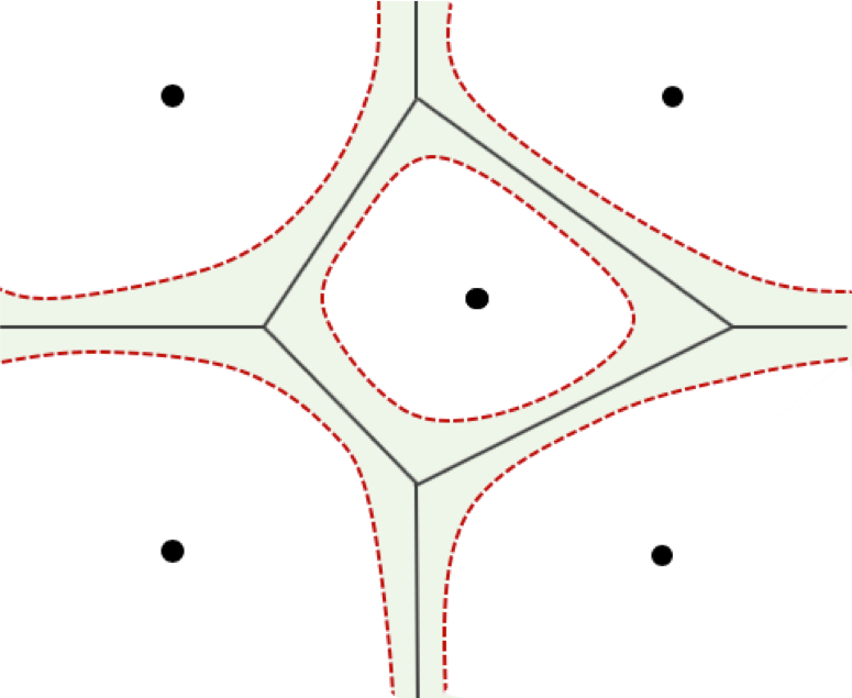
Figure 3: Illustration of the margin condition in Definition 3.1, where we control the probability mass in the shaded area within the red-dashed lines specified by $\kappa$.

$N_{C^{*}}(t)$ can be viewed as a neighborhood of ${\partial C^{*}}$ in which the distance from a point $\mu$ to two nearest cluster centers differs by as much as $t$. For example, in 2-dimensional Euclidean space (i.e., when $p=2$), $N_{C^{*}}(t)$ forms a region surrounded by hyperbolas that are symmetric around each segment in $\{\partial V_{i}(C^{*})=\partial V_{j}(C^{*})\mid i,j\in\{1,\ldots,k\}\}$, as shown in Figure 3. Now we introduce the following margin condition.

Definition 3.1 (Margin condition).

A distribution $\mathbb{P}$ satisfies a margin condition with radius $\kappa>0$ and rate $\alpha>0$ if and only if for all $0\leq t\leq\kappa$,

$$\underset{C^{*}\in\mathcal{C}^{*}_{k}}{\sup}\mathbb{P}(\mu\in N_{C^{*}}(t))\lesssim t^{\alpha}.$$

The above margin condition requires a local control of the probability around $\partial C^{*}$ for $C^{*}\in\mathcal{C}_{k}^{*}$, hence implies that every optimal codebook forms a "natural classification". Levrard (2015, 2018) used the same condition with $\alpha=1$ to achieve fast $O(1/n)$ rates of convergence for the excess risk, and provided some instances of the corresponding natural classifiers. This type of margin condition, where the weight of the neighborhood of the critical region is controlled, has been often adopted for a wide range of problems in causal inference involving estimation of non-smooth target parameters (e.g., van der Laan & Luedtke 2015; Luedtke & Van Der Laan 2016; Kennedy et al. 2018; Levis et al. 2023; Kim & Zubizarreta 2023). We introduce the following mild boundedness and consistency assumptions as well.

Assumption A1.

$\|\mu_{a}\|_{\infty},\|\widehat{\mu}_{a}\|_{\infty}\leq B<\infty$ a.s.

Assumption A2.

$\max_{a}\left\|\widehat{\mu}_{a}-\mu_{a}\right\|_{\infty}=o_{\mathbb{P}}(1)$.

In the next theorem, we give upper bounds of the excess risk, showing that the proposed plug-in estimator (8) is risk consistent.

Theorem 3.1.

Suppose $\mathbb{P}$ satisfies the margin condition with some $\kappa>0$, $\alpha>0$, and let

$$R_{1,n}=\max_{a}\left\|\widehat{\mu}_{a}-\mu_{a}\right\|_{\mathbb{P},1}+\max_{a}\|\widehat{\mu}_{a}-\mu_{a}\|_{\infty}^{\alpha+1}+\frac{1}{\kappa}\max_{a}\left(\|\widehat{\mu}_{a}-\mu_{a}\|_{\infty}\left\|\widehat{\mu}_{a}-\mu_{a}\right\|_{\mathbb{P},1}\right).$$

Then under Assumptions A1, A2, we have

$$\mathbb{P}\left\{R(\widehat{C})-R(C^{*})\right\}=O\left(\frac{1}{\sqrt{n}}+R_{1,n}\right)\quad\text{and}\quad R(\widehat{C})-R(C^{*})=O_{\mathbb{P}}\left(\sqrt{\frac{\log n}{n}}+R_{1,n}\right),$$

whenever $\widehat{\mu}$ is constructed from a separate independent sample.

A proof of the above theorem and all subsequent proofs can be found in Web Appendix B. The term $\|\widehat{\mu}_{a}-\mu_{a}\|_{\infty}^{\alpha+1}$ in $R_{1,n}$ commonly appears in the literature involving efficient estimation of non-smooth functionals based on the margin condition, including those listed above. The term $\frac{1}{\kappa}\left(\|\widehat{\mu}_{a}-\mu_{a}\|_{\infty}\left\|\widehat{\mu}_{a}-\mu_{a}\right\|_{\mathbb{P},1}\right)$ is due to the fact that the margin condition in Definition 3.1 only requires a local control in the neighborhood $N_{C^{*}}(\kappa)$; if $\kappa\rightarrow\infty$, this term vanishes. Theorem 3.1 essentially states that the extra price we pay for excess risk is the estimation error of the outcome regression functions.

The fact that $\widehat{C}$ is risk consistent does not imply that $\widehat{C}$ is actually close to the true codebook $C^{*}$. To assure consistency of $\widehat{C}$, an additional condition is required as follows.

Assumption A3.

$C^{*}$ is unique up to relabeling of its coordinates: i.e., $\mathcal{C}_{k}^{*}$ is a singleton.

The uniqueness specified in Assumption A3 is also used in earlier work by Pollard (1981, 1982). The next theorem states that the proposed plug-in estimator is consistent.

Theorem 3.2.

Under Assumptions A1 - A3, $\widehat{C}$ computed by the plug-in estimator (8) converges in probability to $C^{*}$.

The map $C\mapsto R(C)$ from $\mathbb{R}^{kp}$ into $\mathbb{R}$ is differentiable if $\|\mu\|_{\mathbb{P},2}<\infty$ (Pollard 1982). Based on Theorems 3.1 and 3.2, one may thus characterize the rate of convergence of $\widehat{C}$ as stated in the next corollary.

Corollary 3.3.

Suppose that $\mathbb{P}$ satisfies the margin condition with some $\kappa>0$, $\alpha>0$, and that Assumptions A1 - A3 hold. Also assume that $\widehat{\mu}$ is constructed from a separate independent sample. Then $\|\widehat{C}-C^{*}\|_{1}=\sum_{j=1}^{k}\|\widehat{c}_{j}-c^{*}_{j}\|_{1}=O_{\mathbb{P}}\left(\sqrt{\frac{\log n}{n}}+R_{1,n}\right).$

The plug-in estimator is simple and intuitive. When an initial estimator is available or $\widehat{\mu}$ is fitted in a separate independent sample, (8) is readily implementable using the standard, off-the-shelf algorithms including Lloyd’s algorithm. Otherwise, we can estimate the risk via cross-fitting, where we swap the samples, repeat the procedure, and average the results to regain full sample size efficiency. Then we compute the optimal codebook that minimizes the estimated risk.

Note that the convergence rate in Theorem 3.1 essentially inherits from $\widehat{\mu}$. Hence, for either the risk or the codebook, rates of convergence would be expected to be slower than $\sqrt{n}$ with non-normal limiting distributions not centered at the true parameter, unless careful undersmoothing of particular estimators (e.g., splines) is used. Consequently, valid confidence intervals (even via bootstrap) may not be constructed. In the following section, we will develop an estimator that can be $\sqrt{n}$ consistent and asymptotically normal even if the nuisance functions are estimated flexibly at slower than $\sqrt{n}$ rates, in a wide variety of settings.

4 Semiparametric Estimator

In this section, we describe estimators that achieve faster rates than the plug-in estimator from Section 3 based upon semiparametric efficiency theory.

4.1 Proposed estimator

For convenience, we introduce the following additional notations

$$\pi_{a}(X) =\mathbb{P}\left(A=a\mid X\right),$$ (9)

$$\varphi_{1,a}(Z;\eta_{a}) =\frac{\mathbbm{1}(A=a)}{\pi_{a}(X)}\left\{Y-\mu_{A}(X)\right\}+\mu_{a}(X),$$

$$\varphi_{2,a}(Z;\eta_{a}) =2\mu_{a}(X)\frac{\mathbbm{1}(A=a)}{\pi_{a}(X)}\left\{Y-\mu_{A}(X)\right\}+\mu_{a}^{2}(X),$$

where $\eta_{a}=\{\pi_{a},\mu_{a}\}$ denotes a set of relevant nuisance functions $\forall a$. $\pi_{a}$ is a conditional probability of receiving the treatment $a\in\mathcal{A}$; when $p=2$, $\pi_{1}$ denotes the propensity score. Notice that $\varphi_{1,a}$ and $\varphi_{2,a}$ are the uncentered efficient influence function for the parameters $\mathbb{E}\left\{\mu_{a}(X)\right\}$ and $\mathbb{E}\left\{\mu_{a}^{2}(X)\right\}$, respectively. The efficient influence function is important to construct optimal estimators since its variance equals the efficiency bound (in asymptotic minimax sense). Shortly, we shall see that exploiting the efficient influence function endows our estimators with desirable properties such as double robustness or general second-order bias, allowing us to relax nonparametric conditions on nuisance function estimation. We refer the interested reader to, for example, van der Vaart (2002); Tsiatis (2007); Kennedy (2016, 2022) for more details about influence functions and semiparametric efficiency theory.

Next, for any fixed $C$, we define

$$\varphi_{C}(Z;\eta)=\sum_{a\in\mathcal{A}}\left\{\varphi_{2,a}(Z;\eta_{a})-2\varphi_{1,a}(Z;\eta_{a})\left[\Pi_{C}\left(\mu\right)\right]_{a}+\left[\Pi_{C}\left(\mu\right)\right]^{2}_{a}\right\},$$ (10)

where we let $\eta=\left\{\eta_{a}\right\}_{a\in\mathcal{A}}$ denote a set of all nuisance functions collectively, and $\left[\Pi_{C}\left(\mu\right)\right]_{a}$ be the $a$-th element of the projection $\Pi_{C}\left(\mu\right)$. $\varphi_{C^{*}}(Z;\eta)$ is the uncentered efficient influence function for $R(C^{*})$ whenever $\mathbb{P}$ satisfies the margin condition, as formally stated below.

Lemma 4.1.

Suppose that Assumptions A1, A2 hold, and that $\mathbb{P}$ satisfies the margin condition with some $\kappa>0$ and $\alpha>0$. If, for every optimal codebook $C^{*}\in\mathcal{C}_{k}^{*}$, we let $\phi_{C^{*}}(z;\mathbb{P})=\varphi_{C^{*}}(z;\mathbb{P})-\int\varphi_{C^{*}}(z;\mathbb{P})d\mathbb{P}$, then $\phi_{C^{*}}$ is the efficient influence function for $R(C^{*})$.

We now describe how to construct the proposed estimator for $R(C)$. Following (Robins et al. 2008; Zheng & Van Der Laan 2010; Chernozhukov et al. 2017; Newey & Robins 2018; Kennedy 2023) and many others, we use sample splitting (or cross-fitting) to allow for arbitrarily complex nuisance estimators $\widehat{\eta}$. Specifically with fixed $K$, we split the data into $K$ disjoint groups, each with size $n/K$ approximately, by drawing variables $(B_{1},\ldots,B_{n})$ independent of the data; $B_{i}=b$ indicates that subject $i$ was split into group $b\in\{1,\ldots,K\}$. This could be done, for example, by drawing each $B_{i}$ uniformly from $\{1,\ldots,K\}$. We propose our estimator for $R(C)$ as

$$\widehat{R}(C) =\sum_{b=1}^{K}\left\{\frac{1}{n}\sum_{i=1}^{n}\mathbbm{1}(B_{i}=b)\right\}\mathbb{P}_{n}^{b}\left\{\varphi_{C}(Z;\widehat{\eta}_{-b})\right\}$$

$$\equiv\mathbb{P}_{n}\left\{\varphi_{C}(Z;\widehat{\eta}_{-K})\right\},$$ (11)

where we let $\mathbb{P}_{n}^{b}$ denote empirical averages only over the set of units $\{i:B_{i}=b\}$ in group $b$ and let $\widehat{\eta}_{-b}$ denote the nuisance estimator constructed only using those units $\{i:B_{i}\neq b\}$. In the following section, we will show that the proposed risk estimator $\widehat{R}(C)$ in (4.1) is asymptotically efficient under weak conditions for any $C\in\mathcal{C}^{*}_{k}$.

Then we propose estimating the optimal cluster codebook $C^{*}$ as a minimizer of $\widehat{R}(C)$:

$$\widehat{C}=\underset{C\in\mathcal{C}_{k}}{\mathop{\mathrm{argmin}}}\widehat{R}(C).$$ (12)

After finding the function $\widehat{R}(\cdot)$, $\widehat{C}$ can be computed on a full sample. Note that the cross-fitting procedure described above is equally applicable to the plug-in estimator (8). (12) can be computed using first-order (e.g., gradient descent) or second-order (e.g., Newton-Raphson) methods based on the derivative formulas (13) and (14) specified in the following section.

4.2 Asymptotic Properties

In this subsection, we analyze asymptotic properties of the proposed estimator. For notational simplicity, we define the remainder term that appears in our results as follows:

$$R_{2,n} =\max_{a}\left\{\|\widehat{\mu}_{a}-{\mu}_{a}\|_{\mathbb{P},2}\left(\|\widehat{\mu}_{a}-{\mu}_{a}\|_{\mathbb{P},2}+\|\widehat{\pi}_{a}-{\pi}_{a}\|_{\mathbb{P},2}\right)\right\}+\max_{a}\|\widehat{\mu}_{a}-\mu_{a}\|_{\infty}^{\alpha+1}$$

$$\quad+\frac{1}{\kappa}\max_{a}\left(\|\widehat{\mu}_{a}-\mu_{a}\|_{\infty}\left\|\widehat{\mu}_{a}-\mu_{a}\right\|_{\mathbb{P},1}\right).$$

Note that terms in $R_{2,n}$ are all second-order, as opposed to $R_{1,n}$, the analogous bias term for the plug-in estimator in the previous section. We introduce the following additional assumptions pertaining to our nuisance estimation.

Assumption A4.

$\mathbb{P}\left\{\epsilon\leq\widehat{\pi}_{a}(X)\leq 1-\epsilon\right\}=1$ for some $\epsilon>0$.

Assumption A5.

$\underset{a}{\max}\left\{\|\widehat{\pi}_{a}-{\pi}_{a}\|_{\mathbb{P},2}+\|\widehat{\mu}_{a}-{\mu}_{a}\|_{\infty}\right\}=o_{\mathbb{P}}(1)$.

Assumption A6.

$R_{2,n}=o_{\mathbb{P}}(n^{-1/2})$.

Assumption A5 is a mild consistency assumption, with no requirement on rates of convergence. Assumption A6 may hold, for example, under standard $n^{-1/4}$-type rate conditions on $\widehat{\eta}$ which can be attained under smoothness, sparsity, or other structural constraints (e.g., Kennedy 2016). The next lemma specifies conditions under which $\widehat{R}(C^{*})$ is an asymptotically normal and efficient estimator for $R(C^{*})$.

Lemma 4.2.

Suppose that the margin condition in Definition 3.1 is satisfied with some $\alpha>0$, $\kappa>0$, and that Assumptions A1, A4, A5, and A6 hold. Then for every optimal codebook $C^{*}\in\mathcal{C}_{k}^{*}$,

$$\sqrt{n}\left\{\widehat{R}(C^{*})-R(C^{*})\right\}\leadsto N\left(0,\text{var}\left(\varphi_{C^{*}}\right)\right),$$

where $\varphi_{C}$ is specified in (10).

Under the similar conditions as Theorem 3.2, we can show the proposed codebook estimator (12) is consistent, as stated in the following corollary.

Corollary 4.3.

If Assumptions A1, A3, A4, and A5 hold, then $\widehat{C}$ computed by the semiparametric estimator (12) converges in probability to $C^{*}$.

Based on Lemma 4.2 and Corollary 4.3, in the next theorem we compute an asymptotic bound for the excess risk, as well as the rate of convergence for $\widehat{C}$.

Theorem 4.4.

Suppose that $\mathbb{P}$ satisfies the margin condition with some $\kappa>0$, $\alpha>0$, and that Assumptions A1, A3, A4, and A5 hold. Then,

$$R(\widehat{C})-R(C^{*}) =o_{\mathbb{P}}\left(\frac{1}{\sqrt{n}}+R_{2,n}\right)\quad\text{and}\quad\|\widehat{C}-C^{*}\|_{1}=O_{\mathbb{P}}\left(\frac{1}{\sqrt{n}}+R_{2,n}\right).$$

Theorem 4.4 shows that the proposed codebook estimator $\widehat{C}$ and the associated excess risk may attain substantially faster rates than its nuisance estimators $\widehat{\eta}$. Specifically if $R_{2,n}=O_{\mathbb{P}}\left(n^{-1/2}\right)$ (weaker assumption than A6), we can attain $\sqrt{n}$ rates for $\widehat{C}$ and faster-than-$\sqrt{n}$ rates for excess risk by virtue of the fact that $R_{2,n}$ involves products of nuisance estimation errors.

Asymptotic normality of estimated codebooks in the standard k-means clustering was first studied by Pollard (1982). However, extending the classic result of Pollard (1982) to causal clustering poses some difficulties due to the complexity of our new risk function $\mathbb{E}(\varphi_{C})$ which relies on multiple nuisance components in an infinite-dimensional function space. To achieve asymptotic normality for our estimated codebook $\widehat{C}$, we shall adopt the logic employed in Kennedy et al. (2023).

Let $\upvarphi_{1}(z;\eta)=[\varphi_{1,1}(z;\eta_{1}),\ldots,\varphi_{1,p}(z;\eta_{p})]^{\top}$ where each $\varphi_{1,a}$ is defined in (9). With a slight abuse of notation, as was done in Bottou & Bengio (1994) we compute the derivative of $\varphi_{C}$ at any $C^{\prime}\in\mathcal{C}_{k}$ for some fixed $\bar{\eta}$ by

$$\frac{\partial}{\partial C}\varphi_{C}(Z;\bar{\eta})\Big{|}_{C=C^{\prime}} \equiv\upvarphi_{C^{\prime}}(Z;\bar{\eta})$$ (13)

$$=2\left[(c^{\prime}_{1}-\upvarphi_{1}(Z;\bar{\eta}))\mathbbm{1}\{1=d(\bar{\mu},C^{\prime})\},\ldots,(c^{\prime}_{k}-\upvarphi_{1}(Z;\bar{\eta}))\mathbbm{1}\{k=d(\bar{\mu},C^{\prime})\}\right]^{\top}$$

where we let $d(\bar{\mu},C^{\prime})=\underset{j\in\{1,\ldots,k\}}{\mathop{\mathrm{argmin}}}\|c^{\prime}_{j}-\bar{\mu}\|_{2}^{2}$, i.e., the subscript for the nearest center to a given $\bar{\mu}$. Similarly, one may compute the derivative matrix of $\mathbb{P}\left\{\upvarphi_{C}(Z;\bar{\eta})\right\}$ at $C^{\prime}$:

$$\frac{\partial}{\partial C}\mathbb{P}\left\{\upvarphi_{C}(Z;\bar{\eta})\right\}\Big{|}_{C=C^{\prime}}\equiv M(C^{\prime},\bar{\eta})=2\text{diag}\left(\bm{1}_{(p)}p_{1}(\bar{\eta},C^{\prime}),\ldots,\bm{1}_{(p)}p_{k}(\bar{\eta},C^{\prime})\right),$$ (14)

where $p_{j}(\bar{\eta},C^{\prime})=\mathbb{P}\{j=d(\bar{\mu},C^{\prime})\}$ and $\bm{1}_{(p)}$ is a $p$-dimensional vector of all ones.

Notice that the solutions of the minimization problem (12) can be equivalently expressed by solutions to the following empirical moment condition (up to $o_{\mathbb{P}}(1/\sqrt{n})$ error):

$$\mathbb{P}_{n}\left\{\upvarphi_{\widehat{C}}(Z;\widehat{\eta}_{-K})\right\}=o_{\mathbb{P}}\left(\frac{1}{\sqrt{n}}\right).$$

In the next theorem, we give the main result of this section, which presents conditions allowing for $\sqrt{n}$ consistency and asymptotic normality of $\widehat{C}$ in nonparametric models.

Theorem 4.5.

Suppose that $\mathbb{P}$ satisfies the margin condition with some $\kappa>0$, $\alpha>0$, and that Assumptions A1, A3, A4, and A5 hold. Also, assume that $p_{j}(\eta,C^{*})>0$, $\forall j$. Then,

$$\widehat{C}-C^{*}=-M(C^{*},\eta)^{-1}(\mathbb{P}_{n}-\mathbb{P})\left\{\upvarphi_{C^{*}}(Z;\eta)\right\}+O_{\mathbb{P}}\left(R_{2,n}+o_{\mathbb{P}}\left(\frac{1}{\sqrt{n}}\right)\right).$$

Note that the condition $p_{j}(\eta,C^{*})>0$ is equivalent to $\mathbb{P}\{V_{i}(C^{*})\}>0$, i.e., there are no vacant Voronoi cells, and guarantees that the derivative matrix $M(C^{*},\eta)$ is nonsingular. Importantly, Theorem 4.5 implies that $\widehat{C}$ can be $\sqrt{n}$ consistent and asymptotically normal under the rate condition in Assumption A6, which may hold even when the nuisance estimators are generic and flexibly fit. In this case, asymptotically valid confidence intervals can be readily constructed via bootstrap methods.

5 Illustration

5.1 Simulation Study

In order to assess the performance of the proposed estimators, we conduct a small simulation study. We consider a simplified scenario where a generated codebook forms a natural classifier satisfying the margin condition. As briefly shown in Figure LABEL:fig:experiments-(a), we demonstrate that, as anticipated by our theoretical results, the proposed semiparametric estimator from Section 4 generally has smaller error than the plug-in estimator from Section 3, and achieves parametric $\sqrt{n}$ rates even with $n^{1/4}$ rates on nuisance estimation. Details and full results are included in Web Appendix A.

5.2 Case Study

Here we apply our method to the real-world dataset that was collected to study the relative effects of three treatment programs for adolescent substance abuse, i.e., community ($A=1$), MET&CBT-5 ($A=2$), SCY ($A=3$) (McCaffrey et al. 2013; Burgette et al. 2017). For illustration purpose, we use a subset of publicly available data via the twang R package. The dataset consists of $600$ samples, $200$ youths for each treatment, and $5$ covariates including age, ethnicity, and criminal history. Our outcome is the program effectiveness score, where higher scores indicate reduced frequency of substance use.

We use the proposed semiparametric estimator with $K=2$ splits, using the gradient descent algorithm for optimization. For nonparametric estimation we used the cross-validation-based Super Learner ensemble (Van der Laan et al. 2007) to combine regression splines, support vector machine regression, and random forests. The Elbow method indicates that $k=4$ can be a reasonable choice. Figure LABEL:fig:experiments-(b) displays the four clusters in the counterfactual mean vector space, revealing a substantial degree of heterogeneity. In Figure LABEL:fig:experiments-(c), we also present the density plots for the pairwise CATE estimates $\widehat{\tau}_{2,1}$ and $\widehat{\tau}_{3,1}$, across different clusters. This helps to understand how units in each cluster respond differently to a specific treatment. For instance, for Cluster 2, the traditional community program is more effective than the MET&CBT-5, while there is no significant difference between the community and SCY programs. On the other hand, for units in Cluster 4, the MET&CBT-5 is moderately more successful than the community program, whereas the SCY is significantly less effective.

6 Discussion

In this paper, we propose a new framework for analyzing treatment effect heterogeneity by leveraging tools in cluster analysis. We provide flexible nonparametric estimators for a wide class of models. The proposed methods allow for the discovery of subgroup structure in studies with multiple treatments or outcomes. Our framework is extensible to clustering with generic pseudo-outcomes, such as partially observed outcomes or unknown functionals.

Our findings open up a plethora of intriguing opportunities for future work. In an upcoming companion paper, we consider kernel-based undersmoothing approaches for causal k-means clustering, which do not require the margin condition. Much more work is required to expand causal clustering to other widely-used clustering algorithms, such as density-based clustering and hierarchical clustering. Different algorithms rely on different assumptions about the data, necessitating distinct analysis. Connecting to prescriptive methods, such as optimal treatment regimes, and other settings involving, for example, time-varying treatments, instrumental variables, or mediation would be also promising directions for future research.

Web Appendix

Appendix A Simulation Study Details

We consider a simple data generating process as follows. First, we fix $k,p$, each of which is randomly drawn from a set $\{2,...,10\}$. Then we randomly pick $k$ points in a bounded hypercube $[0,1]^{p}$ under a constraint that every pairwise mutual Euclidean distance between two cluster centers is always greater than $0.2$. A set of these $k$ points is considered as our true codebook $C^{*}=\{c^{*}_{1},...,c^{*}_{k}\}$; consequently $C^{*}$ defines the associated Voronoi cells. To assign roughly equal numbers of units to each $c^{*}_{j}$, for each unit $i=1,...,n$, we draw a label $I\in\{1,...,k\}$ from a multinomial distribution: $I\sim\text{mult}(p_{1},...,p_{k})$ with $p_{1}=\cdots=p_{k}=1/k$. Given this label information, we set $\mu=c^{*}_{I}+\epsilon^{\text{truc}}$ where $\epsilon^{\text{truc}}$ follows a truncated normal distribution of $N(0,1/2)$ with the threshold of $\underset{j}{\min}\,d(c^{*}_{I},c^{*}_{j})/2-0.01$. This guarantees that the nearest center for units with label $j$ in the counterfactual mean vector space is always $c^{*}_{j}$, and that the margin condition holds. Next, we model our observed data generating process by $A\sim\text{mult}(\pi_{1},...,\pi_{p})$ and $Y=\mu_{A}+Z$, where $\pi_{1}=\cdots=\pi_{p}=1/p$ and $Z\sim N(0,1)$. Finally, we let $\widehat{\mu}_{a}=\mu_{a}+\xi$ and $\widehat{\pi}_{a}=\pi_{a}+\zeta$, where $\xi\sim N(0,n^{-(r+0.01)})$ and $\zeta\sim N(0,n^{-(r+0.01)})$, respectively, which ensures that $\|\widehat{\mu}_{a}-\mu_{a}\|=o_{\mathbb{P}}(n^{-r})$ and $\|\widehat{\pi}_{a}-\pi_{a}\|=o_{\mathbb{P}}(n^{-r})$.

We randomly pick $50$ different pairs of $(k,p)$ and vary the sample size $n$ from $250$ to $10,000$ for each $(k,p)$. For each $(k,p,n)$ tuple, we generate data according to the above specified process, and then compute $\widehat{C}$ and the corresponding risk using the plug-in estimator from Section 3, as well as the semiparametric estimator from Section 4. We use $K=2$ splits and the gradient descent algorithm for optimization. We run the simulation $500$ times for each $(k,p,n)$ at two different nuisance rates of $r=1/2,1/4$. Results are presented in Figure LABEL:fig:app-sim.

For both fast ($r=1/2$) and slow ($r=1/4$) rates at which the nuisance functions are estimated, the performance of the proposed semiparametric estimator is improved as $n$ grows, nearly at $n^{1/2}$ rates. On the other hand, the plug-in estimator shows far worse performance at the slow nuisance estimation rates, as it is no longer expected to converge at $n^{1/2}$ rates. Hence, the simulation results validate our theoretical findings in Sections 3 and 4, and support our recommendation to use the proposed semiparametric estimator described in Section 4 in practice.

Appendix B Proofs

Notation Guide. Hereafter, we let $\|f\|$ denote the $L_{2}(\mathbb{P})$-norm in order to simplify notation and avoid any confusion with the Euclidean norm $\|\cdot\|_{2}$, as the $L_{2}(\mathbb{P})$-norm is used most frequently in the proofs. For simplicity, we drop the dependence on $Z$ if the context is clear. Also, for any fixed $C$, we let $f_{C}(x)=\|x-\Pi_{C}(x)\|_{2}^{2}$ for $x\in\mathbb{R}^{p}$ so that $R(C)=\mathbb{E}\{f_{C}(\mu)\}$, and let

$$f_{c_{j}}(\mu) =\|\mu-c_{j}\|_{2}^{2},$$

$$\varphi_{c_{j}}(\eta) =\sum_{a}\left\{\varphi_{2,a}(\eta)-2\varphi_{1,a}(\eta)c_{ja}+c_{ja}^{2}\right\},\quad j=1,\ldots,k.$$

Further, we let $\zeta_{j}(\mu;C)=\underset{j\neq i}{\min}\|\mu-c_{i}\|_{2}-\|\mu-c_{j}\|_{2}$ so that $\mathbb{P}\left\{|\zeta_{j}(\mu;C^{*})|\leq t\bigm{|}0\leq t\leq\kappa\right\}\lesssim t^{\alpha}$ under the margin condition for any $\alpha>0$, $\kappa>0$. With a slight abuse of notation, we write $\|\widehat{C}-C^{*}\|_{1}=\sum_{j=1}^{k}\|\widehat{c}_{j}-c^{*}_{j}\|_{1}$.

B.1 Proof of Theorem 3.1

Before proving Theorem 3.1, we present the three following lemmas.

Lemma B.1.

Suppose that Assumption A1 holds, and $\mathbb{P}$ satisfies the margin condition with some $\kappa>0$, $\alpha>0$. Then we have

$$\mathbb{P}\left|\Pi_{C^{*},a}(\widehat{\mu})-\Pi_{C^{*},a}(\mu)\right| \lesssim\max_{j}\left\|\mathbbm{1}\left\{\zeta_{j}(\widehat{\mu};C^{*})>0\right\}-\mathbbm{1}\left\{\zeta_{j}(\mu;C^{*})>0\right\}\right\|_{\infty}\sum_{a}\|\widehat{\mu}_{a}-\mu_{a}\|_{\mathbb{P},1}$$

$$\quad+\sum_{a}\|\widehat{\mu}_{a}-\mu_{a}\|_{\infty}^{\alpha},$$

where $\Pi_{C^{*},a}(\cdot)$ denotes the $a$-th coordinate of $\Pi_{C^{*}}(\cdot)$.

Proof.

Recall that $\zeta_{j}(\mu;C)=\underset{j\neq i}{\min}\|\mu-c_{i}\|_{2}-\|\mu-c_{j}\|_{2}$. Letting $\zeta_{j}\equiv\zeta_{j}(\mu;C^{*})$ and $\widehat{\zeta}_{j}\equiv\zeta_{j}(\widehat{\mu};C^{*})$, we have

$$\mathbb{P}\left|\Pi_{C^{*},a}(\widehat{\mu})-\Pi_{C^{*},a}(\mu)\right|$$

$$=\mathbb{P}\left(\sum_{j}c^{*}_{j,a}\left|\mathbbm{1}\left\{\widehat{\zeta}_{j}>0\right\}-\mathbbm{1}\left\{\zeta_{j}>0\right\}\right|\right)$$

$$=\sum_{j}c^{*}_{j,a}\mathbb{P}\left(\left|\mathbbm{1}\left\{\widehat{\zeta}_{j}>0\right\}-\mathbbm{1}\left\{\zeta_{j}>0\right\}\right|\left[\mathbbm{1}\left\{\left|\widehat{\zeta}_{j}-\zeta_{j}\right|\leq\kappa\right\}+\mathbbm{1}\left\{\left|\widehat{\zeta}_{j}-\zeta_{j}\right|>\kappa\right\}\right]\right).$$

On the one hand, by the iterated expectation we have that

$$\sum_{j}c^{*}_{j,a}\mathbb{P}\left[\left|\mathbbm{1}\left\{\widehat{\zeta}_{j}>0\right\}-\mathbbm{1}\left\{\zeta_{j}>0\right\}\right|\mathbbm{1}\left\{\left|\widehat{\zeta}_{j}-\zeta_{j}\right|\leq\kappa\right\}\right]$$

$$\leq\sum_{j}c^{*}_{j,a}\mathbb{P}\left[\mathbb{P}\left(\mathbbm{1}\left\{|\zeta_{j}|\leq\left|\widehat{\zeta}_{j}-\zeta_{j}\right|\right\}\Bigm{|}\left|\widehat{\zeta}_{j}-\zeta_{j}\right|\leq\kappa\right)\mathbbm{1}\left\{\left|\widehat{\zeta}_{j}-\zeta_{j}\right|\leq\kappa\right\}\right]$$

$$\leq\sum_{j}c^{*}_{j,a}\mathbb{P}\left[\mathbb{P}\left\{|\zeta_{j}|\leq\left|\widehat{\zeta}_{j}-\zeta_{j}\right|\Bigm{|}\left|\widehat{\zeta}_{j}-\zeta_{j}\right|\leq\kappa\right\}\right]$$

$$\lesssim\sum_{j}\|\widehat{\zeta}_{j}-\zeta_{j}\|_{\infty}^{\alpha}$$

where the last inequality follows by the margin condition. Similarly,

$$\sum_{j}c^{*}_{j,a}\mathbb{P}\left[\left|\mathbbm{1}\left\{\widehat{\zeta}_{j}>0\right\}-\mathbbm{1}\left\{\zeta_{j}>0\right\}\right|\mathbbm{1}\left\{\left|\widehat{\zeta}_{j}-\zeta_{j}\right|>\kappa\right\}\right]$$

$$\leq\sum_{j}c^{*}_{j,a}\left\|\mathbbm{1}\left\{\widehat{\zeta}_{j}>0\right\}-\mathbbm{1}\left\{\zeta_{j}>0\right\}\right\|_{\infty}\mathbb{P}\left[\mathbbm{1}\left\{\left|\widehat{\zeta}_{j}-\zeta_{j}\right|>\kappa\right\}\right]$$

$$\lesssim\sum_{j}c^{*}_{j,a}\left\|\mathbbm{1}\left\{\widehat{\zeta}_{j}>0\right\}-\mathbbm{1}\left\{\zeta_{j}>0\right\}\right\|_{\infty}\left(\sum_{a}\|\widehat{\mu}_{a}-\mu_{a}\|_{\mathbb{P},1}\right),$$

where the first and second inequalities follow by Hölder’s and Markov’s inequalities, respectively, and the fact that each $\zeta_{j}$ is Lipschitz at $\mu$.

Putting the two pieces together, we finally obtain that

$$\mathbb{P}\left|\Pi_{C^{*},a}(\widehat{\mu})-\Pi_{C^{*},a}(\mu)\right|$$

$$\lesssim\max_{j}\left\|\mathbbm{1}\left\{\zeta_{j}(\widehat{\mu};C^{*})>0\right\}-\mathbbm{1}\left\{\zeta_{j}(\mu;C^{*})>0\right\}\right\|_{\infty}\sum_{a}\|\widehat{\mu}_{a}-\mu_{a}\|_{\mathbb{P},1}+\sum_{a}\|\widehat{\mu}_{a}-\mu_{a}\|_{\infty}^{\alpha}.$$

∎

The next lemma shows that one may achieve faster rates for the bias of $f_{C^{*}}(\widehat{\mu})$.

Lemma B.2.

Suppose that Assumption A1 holds and $\mathbb{P}$ satisfies the margin condition with some $\kappa>0$, $\alpha>0$. Then we have

$$\left|\mathbb{P}\left\{f_{C^{*}}(\widehat{\mu})-f_{C^{*}}(\mu)\right\}\right|$$

$$\leq\max_{a}\left\|\widehat{\mu}_{a}-\mu_{a}\right\|_{\mathbb{P},1}+\max_{a}\|\widehat{\mu}_{a}-\mu_{a}\|_{\infty}^{\alpha+1}+\frac{1}{\kappa}\max_{a}\left(\|\widehat{\mu}_{a}-\mu_{a}\|_{\infty}\left\|\widehat{\mu}_{a}-\mu_{a}\right\|_{\mathbb{P},1}\right).$$

Proof.

The proof follows the same logic that we develop in greater detail in the subsequent proof of Lemma B.6 (see Remark B.2). ∎

The following lemma computes the bias of our plug-in risk estimator $\widehat{R}_{n}$.

Lemma B.3.

Suppose $\mathbb{P}$ satisfies the margin condition for some $\kappa>0$, $\alpha>0$. Then under Assumptions A1, A2, we have

$$\widehat{R}_{n}(C^{*})-R(C^{*})$$

$$=O_{\mathbb{P}}\left(\frac{1}{\sqrt{n}}+\max_{a}\left\|\widehat{\mu}_{a}-\mu_{a}\right\|_{\mathbb{P},1}+\max_{a}\|\widehat{\mu}_{a}-\mu_{a}\|_{\infty}^{\alpha+1}+\frac{1}{\kappa}\max_{a}\left(\|\widehat{\mu}_{a}-\mu_{a}\|_{\infty}\left\|\widehat{\mu}_{a}-\mu_{a}\right\|_{\mathbb{P},1}\right)\right),$$

whenever $\widehat{\mu}$ is constructed from a separate independent sample.

Proof.

It is immediate to see that

$$\widehat{R}_{n}(C^{*})-R(C^{*}) =\mathbb{P}_{n}\left\{f_{C^{*}}(\widehat{\mu})\right\}-\mathbb{E}\left\{f_{C^{*}}(\mu)\right\}$$ (A.1)

$$=(\mathbb{P}_{n}-\mathbb{P})\left\{f_{C^{*}}(\widehat{\mu})-f_{C^{*}}(\mu)\right\}$$

$$\quad+(\mathbb{P}_{n}-\mathbb{P})f_{C^{*}}(\mu)+\mathbb{P}\left\{f_{C^{*}}(\widehat{\mu})-f_{C^{*}}(\mu)\right\},$$

where $f_{C}(x)=\|x-\Pi_{C}(x)\|_{2}^{2}$, $\forall x\in\mathbb{R}^{p}$. The central limit theorem implies $(\mathbb{P}_{n}-\mathbb{P})f_{C^{*}}(\mu)=O_{\mathbb{P}}(n^{-1/2})$. Also, it follows by Lemma B.2 that

$$\mathbb{P}\left\{f_{C^{*}}(\widehat{\mu})-f_{C^{*}}(\mu)\right\}$$

$$\leq\max_{a}\left\|\widehat{\mu}_{a}-\mu_{a}\right\|_{\mathbb{P},1}+\max_{a}\|\widehat{\mu}_{a}-\mu_{a}\|_{\infty}^{\alpha+1}+\frac{1}{\kappa}\max_{a}\left(\|\widehat{\mu}_{a}-\mu_{a}\|_{\infty}\left\|\widehat{\mu}_{a}-\mu_{a}\right\|_{\mathbb{P},1}\right).$$

Further, under Assumption A1, it follows that

$$f_{C^{*}}(\widehat{\mu})-f_{C^{*}}(\mu) =\|\widehat{\mu}-\Pi_{C}(\widehat{\mu})\|_{2}^{2}-\|\mu-\Pi_{C}(\mu)\|_{2}^{2}$$

$$=\|\widehat{\mu}\|_{2}^{2}+\widehat{\mu}^{\top}\Pi_{C^{*}}(\widehat{\mu})+\|\Pi_{C^{*}}(\widehat{\mu})\|_{2}^{2}$$

$$\quad-\left\{\|\mu\|_{2}^{2}+\mu^{\top}\Pi_{C^{*}}(\mu)+\|\Pi_{C^{*}}(\mu)\|_{2}^{2}\right\}$$

$$=\|\widehat{\mu}\|_{2}^{2}-\widehat{\mu}^{\top}\Pi_{C^{*}}(\widehat{\mu})+\widehat{\mu}^{\top}\Pi_{C^{*}}(\mu)+\|\Pi_{C^{*}}(\widehat{\mu})\|_{2}^{2}$$

$$\quad-\left\{\|\mu\|_{2}^{2}-\mu^{\top}\Pi_{C^{*}}(\mu)+\widehat{\mu}^{\top}\Pi_{C^{*}}(\mu)+\|\Pi_{C^{*}}(\mu)\|_{2}^{2}\right\}$$

$$\leq 3B\sum_{a}\left\{\left|\widehat{\mu}_{a}-\mu_{a}\right|+\left|\Pi_{C^{*},a}(\widehat{\mu})-\Pi_{C^{*},a}(\mu)\right|\right\},$$ (A.2)

which, by the triangle inequality, leads to

$$\|f_{C^{*}}(\widehat{\mu})-f_{C^{*}}(\mu)\|\lesssim\sum_{a}\left(\|\widehat{\mu}_{a}-\mu_{a}\|+\left\|\Pi_{C^{*},a}(\widehat{\mu})-\Pi_{C^{*},a}(\mu)\right\|\right).$$

For the second term in the last display, note that

$$\mathbb{P}\left\{\Pi_{C^{*},a}(\widehat{\mu})-\Pi_{C^{*},a}(\mu)\right\}^{2} =\mathbb{P}\left(\sum_{j}c^{*}_{j,a}\left[\mathbbm{1}\left\{\zeta_{j}(\widehat{\mu})>0\right\}-\mathbbm{1}\left\{\zeta_{j}(\mu)>0\right\}\right]\right)^{2}$$

$$\leq\mathbb{P}\left\{\sum_{j}{c^{*}}_{j,a}^{2}\sum_{j}\left[\mathbbm{1}\left\{\zeta_{j}(\widehat{\mu})>0\right\}-\mathbbm{1}\left\{\zeta_{j}(\mu)>0\right\}\right]^{2}\right\}$$

$$\lesssim\sum_{j}c^{*}_{j,a}\mathbb{P}\left|\mathbbm{1}\left\{\zeta_{j}(\widehat{\mu})>0\right\}-\mathbbm{1}\left\{\zeta_{j}(\mu)>0\right\}\right|$$

$$\lesssim\max_{j}\left\|\mathbbm{1}\left\{\zeta_{j}(\widehat{\mu};C^{*})>0\right\}-\mathbbm{1}\left\{\zeta_{j}(\mu;C^{*})>0\right\}\right\|_{\infty}\sum_{a}\|\widehat{\mu}_{a}-\mu_{a}\|_{\mathbb{P},1}$$

$$\quad+\sum_{a}\|\widehat{\mu}_{a}-\mu_{a}\|_{\infty}^{\alpha},$$ (A.3)

where the last inequality follows by Lemma B.1. Hence, by the given consistency condition in Assumption A2, we get $\|\widehat{\mu}_{a}-\mu_{a}\|_{\mathbb{P},1}=o_{\mathbb{P}}(1)$, $\|\widehat{\mu}_{a}-\mu_{a}\|_{\infty}^{\alpha}=o_{\mathbb{P}}(1)$, $\forall\alpha>0$, and thereby conclude that $\left\|\Pi_{C^{*},a}(\widehat{\mu})-\Pi_{C^{*},a}(\mu)\right\|=o_{\mathbb{P}}(1)$. Hence, $\|f_{C^{*}}(\widehat{\mu})-f_{C^{*}}(\mu)\|=o_{\mathbb{P}}(1)$, and by the sample splitting lemma (Kennedy et al. 2018, Lemma 2), we obtain $(\mathbb{P}_{n}-\mathbb{P})\left\{f_{C^{*}}(\widehat{\mu})-f_{C^{*}}(\mu)\right\}=o_{\mathbb{P}}(n^{-1/2})$.

Putting the three pieces back together into (A.1), we obtain the desired bias bound as

$$\widehat{R}_{n}(C^{*})-R(C^{*})$$

$$=O_{\mathbb{P}}\left(\frac{1}{\sqrt{n}}+\max_{a}\left\|\widehat{\mu}_{a}-\mu_{a}\right\|_{\mathbb{P},1}+\max_{a}\|\widehat{\mu}_{a}-\mu_{a}\|_{\infty}^{\alpha+1}+\frac{1}{\kappa}\max_{a}\left(\|\widehat{\mu}_{a}-\mu_{a}\|_{\infty}\left\|\widehat{\mu}_{a}-\mu_{a}\right\|_{\mathbb{P},1}\right)\right).$$

∎

Theorem 3.1 immediately follows by Lemma B.3.

Proof of Theorem 3.1.

Notice that

$$R(\widehat{C})-R(C^{*}) =R(\widehat{C})-\widehat{R}_{n}(\widehat{C})+\widehat{R}_{n}(\widehat{C})-R(C^{*})$$

$$\leq R(\widehat{C})-\widehat{R}_{n}(\widehat{C})+\widehat{R}_{n}(C^{*})-R(C^{*})$$

$$\leq\underset{C\in\mathcal{C}_{k}}{\sup}\left|R(C)-\widehat{R}_{n}(C)\right|+\widehat{R}_{n}(C^{*})-R(C^{*}).$$ (A.4)

Since $\left\|\mu\right\|_{2}<\infty$ a.s., Linder et al. (1994, Theorem 1) implies the following bound for the first term in (B.1):

$$\underset{C\in\mathcal{C}_{k}}{\sup}\left|R(C)-R_{n}(C)\right|=O_{\mathbb{P}}\left(\sqrt{\frac{\log n}{n}}\right)$$ (A.5)

For the second term, we have

$$\widehat{R}_{n}(C^{*})-R(C^{*})$$

$$=O_{\mathbb{P}}\left(\frac{1}{\sqrt{n}}+\max_{a}\left\|\widehat{\mu}_{a}-\mu_{a}\right\|_{\mathbb{P},1}+\max_{a}\|\widehat{\mu}_{a}-\mu_{a}\|_{\infty}^{\alpha+1}+\frac{1}{\kappa}\max_{a}\left(\|\widehat{\mu}_{a}-\mu_{a}\|_{\infty}\left\|\widehat{\mu}_{a}-\mu_{a}\right\|_{\mathbb{P},1}\right)\right),$$ (A.6)

due to Lemma B.3.

Hence we obtain that

$$R(\widehat{C})-R(C^{*})$$

$$=O_{\mathbb{P}}\left(\sqrt{\frac{\log n}{n}}+\max_{a}\left\|\widehat{\mu}_{a}-\mu_{a}\right\|_{\mathbb{P},1}+\max_{a}\|\widehat{\mu}_{a}-\mu_{a}\|_{\infty}^{\alpha+1}+\frac{1}{\kappa}\max_{a}\left(\|\widehat{\mu}_{a}-\mu_{a}\|_{\infty}\left\|\widehat{\mu}_{a}-\mu_{a}\right\|_{\mathbb{P},1}\right)\right).$$

The same argument as in the preceding proof can be used to compute the rate of convergence in expectation as well. Specifically, when $\|\mu\|_{\infty}\leq B<\infty$ a.s., Biau et al. (2008, Theorem 2.1) implies that

$$\mathbb{P}\left\{\underset{C\in\mathcal{C}_{k}}{\sup}\left|R(C)-R_{n}(C)\right|\right\} \leq\frac{12B^{2}k}{\sqrt{n}}.$$

Also, by virtue of Lemma B.2 one may deduce that

$$\mathbb{P}\left\{\widehat{R}_{n}(C^{*})-R(C^{*})\right\} =\mathbb{P}\left\{f_{C^{*}}(\widehat{\mu})-f_{C^{*}}(\mu)\right\}$$

$$\lesssim\max_{a}\left\|\widehat{\mu}_{a}-\mu_{a}\right\|_{\mathbb{P},1}+\max_{a}\|\widehat{\mu}_{a}-\mu_{a}\|_{\infty}^{\alpha+1}+\frac{1}{\kappa}\max_{a}\left(\|\widehat{\mu}_{a}-\mu_{a}\|_{\infty}\left\|\widehat{\mu}_{a}-\mu_{a}\right\|_{\mathbb{P},1}\right).$$

Using the above inequalities instead of (A.5) and (B.1), we obtain that

$$\mathbb{P}\left\{R(\widehat{C})-R(C^{*})\right\}$$

$$\lesssim\frac{1}{\sqrt{n}}+\max_{a}\left\|\widehat{\mu}_{a}-\mu_{a}\right\|_{\mathbb{P},1}+\max_{a}\|\widehat{\mu}_{a}-\mu_{a}\|_{\infty}^{\alpha+1}+\frac{1}{\kappa}\max_{a}\left(\|\widehat{\mu}_{a}-\mu_{a}\|_{\infty}\left\|\widehat{\mu}_{a}-\mu_{a}\right\|_{\mathbb{P},1}\right).$$

∎

B.2 Proof of Theorem 3.2

Lemma B.4.

For any $C\in\mathcal{C}_{k}$, under Assumption A1, we have

$$\underset{C\in\mathcal{C}_{k}}{\sup}\left|\mathbb{P}\left\{f_{C}(\widehat{\mu})-f_{C}(\mu)\right\}\right|\lesssim\max_{a}\|\widehat{\mu}_{a}-\mu_{a}\|_{\mathbb{P},1}.$$

Proof.

We defer the proof until Lemma B.7 (see Remark B.3). ∎

First, we aim to show

$$\underset{C\in\mathcal{C}_{k}}{\sup}\left|R_{n}(C)-R(C)\right|=o_{\mathbb{P}}(1).$$

To this end, consider the following decomposition for any $C\in\mathcal{C}_{k}$:

$$R_{n}(C)-R(C) =\underbrace{(\mathbb{P}_{n}-\mathbb{P})\left\{f_{C}(\widehat{\mu})-f_{C}(\mu)\right\}}_{(i)}$$

$$\quad+\underbrace{\mathbb{P}\left\{f_{C}(\widehat{\mu})-f_{C}(\mu)\right\}}_{(ii)}$$

$$\quad+\underbrace{(\mathbb{P}_{n}-\mathbb{P})\left\{f_{C}(\mu)\right\}}_{(iii)}.$$

We will analyze the terms in the following order: (iii) $\rightarrow$ (ii) $\rightarrow$ (i).

(iii) Consider sets $\mathscrsfs{G}$ of the subgraph $\{f_{C}(x)>u:(x,u)\in\mathbb{R}^{p}\times\mathbb{R}\}$. The shattering number of $\mathscrsfs{G}$ is $s(\mathscrsfs{G},n)\leq n^{k(p+1)}$, which follows by the fact that each $\{f_{C}(x)>u\}$ is represented as a union of the complements of $k$ spheres. Hence the function class $\widetilde{\mathcal{F}}=\{f_{C}(\cdot):C\in\mathcal{C}_{k}\}$ is a VC-class. For any fixed $\mu:\mathbb{R}^{p}\to\mathbb{R}$ and $f_{C}(\mu)=\|\mu-\Pi_{C}(\mu)\|_{2}^{2}=f_{C}\circ\mu$, by the stability property (e.g., Van Der Vaart & Wellner 1996, Lemma 2.6.17) the function class $\mathcal{F}_{\mu}=\{f_{C}(\mu(\cdot)):C\in\mathcal{C}_{k}\}$ is also a VC-class. Taking $F_{\mu}=\underset{C\in\mathcal{C}_{k}}{\sup}\left|f_{C}(\mu)\right|$ as the envelope function, we have $\mathbb{P}\{F_{\mu}\}\leq 4B^{2}$ under the given boundedness condition. Thus, $\mathcal{F}_{\mu}$ is $\mathbb{P}$-Glivenko-Cantelli, yielding $\underset{C\in\mathcal{C}_{k}}{\sup}\left|(\mathbb{P}_{n}-\mathbb{P})\left\{f_{C}(\mu)\right\}\right|=o_{\mathbb{P}}(1)$.

(ii) Under Assumption A1, by Lemma B.4 we have

$$\underset{C\in\mathcal{C}_{k}}{\sup}\left|\mathbb{P}\left\{f_{C}(\widehat{\mu})-f_{C}(\mu)\right\}\right|\lesssim\max_{a}\|\widehat{\mu}_{a}-\mu_{a}\|_{\infty},$$

which is $o_{\mathbb{P}}(1)$ under the consistency condition in Assumptions A2.

(i) Let $\mathcal{F}_{n}=\mathcal{F}_{\hat{\mu}}-\mathcal{F}_{\mu}$ for the function class $\mathcal{F}_{\bar{\mu}}=\{f_{C}(\bar{\mu}(\cdot)):C\in\mathcal{C}_{k}\}$ from before. Then,

$$\left\|\frac{1}{\sqrt{n}}\mathbb{G}_{n}\left\{f_{C}(\widehat{\mu})-f_{C}(\mu)\right\}\right\|_{\mathcal{C}_{k}} =\underset{C\in\mathcal{C}_{k}}{\sup}\left|\frac{1}{\sqrt{n}}\mathbb{G}_{n}\left\{f_{C}(\widehat{\mu})-f_{C}(\mu)\right\}\right|$$

$$=\frac{1}{\sqrt{n}}\underset{f\in\mathcal{F}_{n}}{\sup}\left|\mathbb{G}_{n}(f)\right|.$$

One may view the nuisance functions $\widehat{\mu}$ as fixed given the training data $D_{0}$. Since $\mathcal{F}_{\mu}$ is a VC-subgraph for any fixed $\mu$, so is $\mathcal{F}_{n}$ given $D_{0}$. Let the VC index of $\mathcal{F}_{n}$ be $\nu^{\prime}<\infty$. Then we have

$$\underset{Q}{\sup}N\left(\epsilon\|F_{n}\|_{Q,2},\mathcal{F}_{n},L_{2}(Q)\right)\lesssim\left(\frac{c_{1}}{\epsilon}\right)^{c_{2}\nu^{\prime}}$$

for some universal constants $c_{1},c_{2}>0$. Hence applying Giné & Nickl (2021, Theorem 3.5.4), we obtain that

$$\mathbb{P}\left\{\underset{f\in\mathcal{F}_{n}}{\sup}\left|\mathbb{G}_{n}(f)\right|\right\} \lesssim\left\|F_{n}\right\|\underset{Q}{\sup}\int_{0}^{1}\sqrt{1+\log N\left(\epsilon\|F_{n}\|_{Q,2},\mathcal{F}_{n},L_{2}(Q)\right)}d\epsilon$$

$$\lesssim\left\|F_{n}\right\|\int_{0}^{1}\sqrt{1+\nu^{\prime}\log(1/\epsilon)}d\epsilon.$$

Taking the envelope $F_{n}=\underset{C\in\mathcal{C}_{k}}{\sup}\left|f_{C}(\widehat{\mu})-f_{C}(\mu)\right|$ which is bounded, it is immediate to show that $\mathbb{P}\left\{\underset{f\in\mathcal{F}_{n}^{b}}{\sup}\left|\mathbb{G}_{n}(f)\right|\right\}=O_{\mathbb{P}}(1)$ as the integral in the last display is finite. Consequently we get $\left\|(\mathbb{P}_{n}-\mathbb{P})\left\{f_{C}(\widehat{\mu})-f_{C}(\mu)\right\}\right\|_{\mathcal{C}_{k}}=O_{\mathbb{P}}(\frac{1}{\sqrt{n}})=o_{\mathbb{P}}(1)$.

Now that we have shown $\underset{C\in\mathcal{C}_{k}}{\sup}\left|\widehat{R}(C)-R(C)\right|=o_{\mathbb{P}}(1),$ the desired consistency $\widehat{C}\xrightarrow{p}C^{*}$ follows by Van der Vaart (2000, Theorem 5.7), noting that $R(\cdot)$ is a continuous, bounded function whose domain $\mathcal{C}_{k}$ is compact, and that $C^{*}$ is unique.

B.3 Proof of Lemma 4.1

Before proving the main result, we introduce the following lemma.

Lemma B.5.

Under Assumptions A1 and A4, we have that for any $a\in\mathcal{A}$,

$$\mathbb{P}\left\{\varphi_{2,a}(\widehat{\eta})-\varphi_{2,a}(\eta)\right\}\lesssim\|\widehat{\mu}_{a}-{\mu}_{a}\|\left(\|\widehat{\mu}_{a}-{\mu}_{a}\|+\|\widehat{\pi}_{a}-{\pi}_{a}\|\right).$$

Proof.

Since $\mathbb{P}\left\{\varphi_{2,a}(\eta)\right\}=\mathbb{P}\left\{\mu_{a}^{2}(X)\right\}$, it follows

$$\mathbb{P}\left\{\varphi_{2,a}(\widehat{\eta})-\varphi_{2,a}(\eta)\right\} =\mathbb{P}\left\{2\widehat{\mu}_{a}\frac{\mathbbm{1}(A=a)}{\widehat{\pi}_{a}}\left\{Y-\widehat{\mu}_{A}\right\}+\widehat{\mu}_{a}^{2}-\mu_{a}^{2}\right\}$$

$$=\mathbb{P}\left\{2\widehat{\mu}_{a}\frac{\pi_{a}}{\widehat{\pi}_{a}}(\mu_{a}-\widehat{\mu}_{a})+(\widehat{\mu}_{a}-\mu_{a})(\widehat{\mu}_{a}+\mu_{a})\right\}$$

$$=\mathbb{P}\left[\left(\mu_{a}-\widehat{\mu}_{a}\right)\left\{4\widehat{\mu}_{a}\left(\frac{\pi_{a}-\widehat{\pi}_{a}}{\widehat{\pi}_{a}}\right)+\widehat{\mu}_{a}-{\mu}_{a}\right\}\right]$$

$$\leq\mathbb{P}\left\{\left|\widehat{\mu}_{a}-{\mu}_{a}\right|\left(\left|\widehat{\mu}_{a}-{\mu}_{a}\right|+\frac{4B}{\epsilon}\left|\widehat{\pi}_{a}-{\pi}_{a}\right|\right)\right\}$$

$$\lesssim\left\|\widehat{\mu}_{a}-{\mu}_{a}\right\|\left(\left\|\widehat{\mu}_{a}-{\mu}_{a}\right\|+\left\|\widehat{\pi}_{a}-{\pi}_{a}\right\|\right)$$

∎

Remark B.1.

(Kennedy (2022, Example 2)) For $\varphi_{1,a}(\eta)$, it is well known that

$$\mathbb{P}\left\{\varphi_{1,a}(\widehat{\eta})-\varphi_{1,a}(\eta)\right\}\lesssim\|\widehat{\mu}_{a}-{\mu}_{a}\|\|\widehat{\pi}_{a}-{\pi}_{a}\|.$$

Lemma B.6.

Suppose that Assumptions A1, A4 hold and $\mathbb{P}$ satisfies the margin condition with some $\kappa>0$, $\alpha>0$. Then we have

$$\left|\mathbb{P}\left\{\varphi_{C^{*}}(\widehat{\eta})-\varphi_{C^{*}}(\eta)\right\}\right|$$

$$\lesssim\max_{a}\left\|\widehat{\mu}_{a}-{\mu}_{a}\right\|\left(\left\|\widehat{\mu}_{a}-{\mu}_{a}\right\|+\left\|\widehat{\pi}_{a}-{\pi}_{a}\right\|\right)+\max_{a}\|\widehat{\mu}_{a}-\mu_{a}\|_{\infty}^{\alpha+1}$$

$$\quad+\frac{1}{\kappa}\max_{a}\left(\|\widehat{\mu}_{a}-\mu_{a}\|_{\infty}\left\|\widehat{\mu}_{a}-\mu_{a}\right\|_{\mathbb{P},1}\right).$$

Proof.

Letting

$$f_{c^{*}_{j}}(\mu) =\|\mu-c^{*}_{j}\|_{2}^{2},$$

$$\varphi_{c^{*}_{j}}(\eta) =\sum_{a}\left\{\varphi_{2,a}(\eta)-2\varphi_{1,a}(\eta)c^{*}_{ja}+{c^{*}}_{ja}^{2}\right\},$$

and

$$d\equiv d(\mu;C^{*}) =\mathop{\mathrm{argmin}}_{j}f_{c^{*}_{j}}(\mu),$$

$$\widehat{d}\equiv d(\widehat{\mu};C^{*}) =\mathop{\mathrm{argmin}}_{j}f_{c^{*}_{j}}(\widehat{\mu}),$$

one may write

$$\mathbb{P}\left\{f_{C^{*}}(\mu)\right\} =\mathbb{P}\left[\min_{j\in\{1,\ldots,k\}}f_{c^{*}_{j}}(\mu)\right]=\sum_{j=1}^{k}\mathbb{P}\left\{\mathbbm{1}\{d=j\}f_{c^{*}_{j}}(\mu)\right\},$$

$$\mathbb{P}\{\varphi_{C^{*}}(\eta)\} =\sum_{j=1}^{k}\mathbb{P}\left\{\mathbbm{1}\{d=j\}\varphi_{c^{*}_{j}}(\eta)\right\},$$

$$\mathbb{P}\{\varphi_{C^{*}}(\widehat{\eta})\} =\sum_{j=1}^{k}\mathbb{P}\left\{\mathbbm{1}\{\widehat{d}=j\}\varphi_{c^{*}_{j}}(\widehat{\eta})\right\}.$$

Now note that

$$\mathbb{P}\left\{\varphi_{C^{*}}(\widehat{\eta})-\varphi_{C^{*}}(\eta)\right\}$$

$$=\sum_{j=1}^{k}\left(\mathbb{P}\left[\mathbbm{1}(\widehat{d}=j)\left\{\varphi_{c^{*}_{j}}(\widehat{\eta})-\varphi_{c^{*}_{j}}(\eta)\right\}\right]+\mathbb{P}\left[\left\{\mathbbm{1}(\widehat{d}=j)-\mathbbm{1}(d=j)\right\}\varphi_{c^{*}_{j}}(\eta)\right]\right)$$

$$=\sum_{j=1}^{k}\left(\mathbb{P}\left[\mathbbm{1}(\widehat{d}=j)\left\{\varphi_{c^{*}_{j}}(\widehat{\eta})-\varphi_{c^{*}_{j}}(\eta)\right\}\right]+\mathbb{P}\left[\left\{\mathbbm{1}(\widehat{d}=j)-\mathbbm{1}(d=j)\right\}f_{c^{*}_{j}}(\mu)\right]\right),$$ (A.7)

where the last equality follows by the fact that $\mathbb{P}\left\{f_{C^{*}}(\mu)\right\}=\mathbb{P}\{\varphi_{C^{*}}(\eta)\}$. For the first term in the last display, it is immediate to see by Lemma B.5 and Remark B.1 that

$$\sum_{j=1}^{k}\left|\mathbb{P}\left[\mathbbm{1}(\widehat{d}=j)\left\{\varphi_{c^{*}_{j}}(\widehat{\eta})-\varphi_{c^{*}_{j}}(\eta)\right\}\right]\right|\lesssim\max_{a}\left\|\widehat{\mu}_{a}-{\mu}_{a}\right\|\left(\left\|\widehat{\mu}_{a}-{\mu}_{a}\right\|+\left\|\widehat{\pi}_{a}-{\pi}_{a}\right\|\right).$$ (A.8)

Next, let us rewrite the second term in (A.7) by

$$\sum_{j}\mathbb{P}\left[\left\{\mathbbm{1}(\widehat{d}=j)-\mathbbm{1}(d=j)\right\}f_{c^{*}_{j}}(\mu)\right]$$

$$=\sum_{j}\mathbb{P}\Bigg{(}\left\{\mathbbm{1}(\widehat{d}=j)-\mathbbm{1}(d=j)\right\}f_{c^{*}_{j}}(\mu)$$

$$\qquad\qquad\times\left[\mathbbm{1}\left\{2\max_{j}\left|f_{c^{*}_{j}}(\widehat{\mu})-f_{c^{*}_{j}}(\mu)\right|\leq\kappa\right\}+\mathbbm{1}\left\{2\max_{j}\left|f_{c^{*}_{j}}(\widehat{\mu})-f_{c^{*}_{j}}(\mu)\right|>\kappa\right\}\right]\Bigg{)}.$$

By mimicking the proof of Theorem 2 in Levis et al. (2023), we have that

$$\left|\sum_{j}\mathbb{P}\left[\left\{\mathbbm{1}(\widehat{d}=j)-\mathbbm{1}(d=j)\right\}f_{c^{*}_{j}}(\mu)\mathbbm{1}\left\{2\max_{j}\left|f_{c^{*}_{j}}(\widehat{\mu})-f_{c^{*}_{j}}(\mu)\right|\leq\kappa\right\}\right]\right|$$

$$=\mathbb{P}\left[\mathbbm{1}\left\{f_{c^{*}_{d}}(\mu)<f_{c^{*}_{\widehat{d}}}(\mu)\right\}\left\{f_{c^{*}_{\widehat{d}}}(\mu)-f_{c^{*}_{d}}(\mu)\right\}\mathbbm{1}\left\{2\max_{j}\left|f_{c^{*}_{j}}(\widehat{\mu})-f_{c^{*}_{j}}(\mu)\right|\leq\kappa\right\}\right]$$

$$\leq\mathbb{P}\Bigg{(}\mathbbm{1}\left[\min_{j\neq d}\left\{f_{c^{*}_{j}}(\mu)-f_{c^{*}_{d}}(\mu)\right\}\leq f_{c^{*}_{\widehat{d}}}(\mu)-f_{c^{*}_{d}}(\mu)+f_{c^{*}_{d}}(\widehat{\mu})-f_{c^{*}_{\widehat{d}}}(\widehat{\mu})\right]$$

$$\qquad\quad\times\left\{f_{c^{*}_{\widehat{d}}}(\mu)-f_{c^{*}_{d}}(\mu)+f_{c^{*}_{d}}(\widehat{\mu})-f_{c^{*}_{\widehat{d}}}(\widehat{\mu})\right\}\mathbbm{1}\left\{2\max_{j}\left|f_{c^{*}_{j}}(\widehat{\mu})-f_{c^{*}_{j}}(\mu)\right|\leq\kappa\right\}\Bigg{)}$$

$$\leq 2\max_{j}\|f_{c^{*}_{j}}(\widehat{\mu})-f_{c^{*}_{j}}(\mu)\|_{\infty}$$

$$\quad\times\mathbb{P}\left[\zeta_{j}(\mu;C^{*})\leq 2\max_{j}\left|f_{c^{*}_{j}}(\widehat{\mu})-f_{c^{*}_{j}}(\mu)\right|\Bigm{|}2\max_{j}\left|f_{c^{*}_{j}}(\widehat{\mu})-f_{c^{*}_{j}}(\mu)\right|\leq\kappa\right]$$

$$\lesssim\max_{j}\|f_{c^{*}_{j}}(\widehat{\mu})-f_{c^{*}_{j}}(\mu)\|_{\infty}^{\alpha+1}$$

$$\lesssim\max_{a}\|\widehat{\mu}_{a}-\mu_{a}\|_{\infty}^{\alpha+1},$$ (A.9)

where the first inequality follows by the fact that $f_{c^{*}_{d}}(\widehat{\mu})\geq f_{c^{*}_{\widehat{d}}}(\widehat{\mu})$ and $f_{c^{*}_{\widehat{d}}}(\mu)\geq f_{c^{*}_{d}}(\mu)$, the third by the margin condition, and the last by local Lipschitz continuity of each $f_{c^{*}_{j}}$ at $\mu$ under Assumption A1.

Similarly as above, we also note that

$$\left|\sum_{j}\mathbb{P}\left[\left\{\mathbbm{1}(\widehat{d}=j)-\mathbbm{1}(d=j)\right\}f_{C^{*}}(\mu)\mathbbm{1}\left\{2\max_{j}\left|f_{c^{*}_{j}}(\widehat{\mu})-f_{c^{*}_{j}}(\mu)\right|>\kappa\right\}\right]\right|$$

$$=\mathbb{P}\left[\mathbbm{1}\left\{f_{c^{*}_{d}}(\mu)<f_{c^{*}_{\widehat{d}}}(\mu)\right\}\left\{f_{c^{*}_{\widehat{d}}}(\mu)-f_{c^{*}_{d}}(\mu)\right\}\mathbbm{1}\left\{2\max_{j}\left|f_{c^{*}_{j}}(\widehat{\mu})-f_{c^{*}_{j}}(\mu)\right|>\kappa\right\}\right]$$

$$\leq\mathbb{P}\left[\mathbbm{1}\left\{f_{c^{*}_{d}}(\mu)<f_{c^{*}_{\widehat{d}}}(\mu)\right\}\left\{f_{c^{*}_{\widehat{d}}}(\mu)-f_{c^{*}_{d}}(\mu)+f_{c^{*}_{d}}(\widehat{\mu})-f_{c^{*}_{\widehat{d}}}(\widehat{\mu})\right\}\mathbbm{1}\left\{2\max_{j}\left|f_{c^{*}_{j}}(\widehat{\mu})-f_{c^{*}_{j}}(\mu)\right|>\kappa\right\}\right]$$

$$\leq 2\max_{j}\|f_{c^{*}_{j}}(\widehat{\mu})-f_{c^{*}_{j}}(\mu)\|_{\infty}\mathbb{P}\left\{\max_{j}\left|f_{c^{*}_{j}}(\widehat{\mu})-f_{c^{*}_{j}}(\mu)\right|>\kappa/2\right\}$$

$$\leq\frac{4}{\kappa}\max_{j}\|f_{c^{*}_{j}}(\widehat{\mu})-f_{c^{*}_{j}}(\mu)\|_{\infty}\max_{j}\mathbb{P}\left|f_{c^{*}_{j}}(\widehat{\mu})-f_{c^{*}_{j}}(\mu)\right|$$

$$\lesssim\frac{1}{\kappa}\max_{a}\|\widehat{\mu}_{a}-\mu_{a}\|_{\infty}\left\|\widehat{\mu}_{a}-\mu_{a}\right\|_{\mathbb{P},1},$$ (A.10)

which the first inequality follow by Hölder’s inequality, the second by Markov’s inequality. Putting these together, we finally obtain that

$$\left|\mathbb{P}\left\{\varphi_{C^{*}}(\widehat{\eta})-\varphi_{C^{*}}(\eta)\right\}\right|$$

$$\lesssim\max_{a}\left\|\widehat{\mu}_{a}-{\mu}_{a}\right\|\left(\left\|\widehat{\mu}_{a}-{\mu}_{a}\right\|+\left\|\widehat{\pi}_{a}-{\pi}_{a}\right\|\right)+\max_{a}\|\widehat{\mu}_{a}-\mu_{a}\|_{\infty}^{\alpha+1}$$

$$\quad+\frac{1}{\kappa}\max_{a}\|\widehat{\mu}_{a}-\mu_{a}\|_{\infty}\left\|\widehat{\mu}_{a}-\mu_{a}\right\|_{\mathbb{P},1}.$$

∎

Remark B.2 (Proof of Lemma B.2).

The proof of Lemma B.2 parallels the proof of Lemma B.6 provided above. Indeed, since we have the counterpart of (A.7) as

$$\mathbb{P}\left\{f_{C^{*}}(\widehat{\mu})-f_{C^{*}}(\mu)\right\}$$

$$=\sum_{j=1}^{k}\left(\mathbb{P}\left[\mathbbm{1}(\widehat{d}=j)\left\{f_{c^{*}_{j}}(\widehat{\mu})-f_{c^{*}_{j}}(\mu)\right\}\right]+\mathbb{P}\left[\left\{\mathbbm{1}(\widehat{d}=j)-\mathbbm{1}(d=j)\right\}f_{c^{*}_{j}}(\mu)\right]\right),$$

the only difference is to replace (A.8) with

$$\sum_{j=1}^{k}\left|\mathbb{P}\left[\mathbbm{1}(\widehat{d}=j)\left\{f_{c^{*}_{j}}(\widehat{\mu})-f_{c^{*}_{j}}(\mu)\right\}\right]\right|\lesssim\max_{a}\left\|\widehat{\mu}_{a}-{\mu}_{a}\right\|_{\mathbb{P},1},$$

which gives the result.

Using the same logic as in the proof of Lemma B.6, we may obtain the following uniform bound.

Lemma B.7.

For any $C\in\mathcal{C}_{k}$, under Assumptions A1, A4, we have

$$\underset{C\in\mathcal{C}_{k}}{\sup}\left|\mathbb{P}\left\{\varphi_{C}(\widehat{\eta})-\varphi_{C}(\eta)\right\}\right| \lesssim\max_{a}\|\widehat{\mu}_{a}-\mu_{a}\|_{\mathbb{P},1}+\max_{a}\left\|\widehat{\mu}_{a}-{\mu}_{a}\right\|\left(\left\|\widehat{\mu}_{a}-{\mu}_{a}\right\|+\left\|\widehat{\pi}_{a}-{\pi}_{a}\right\|\right).$$

Proof.

Notice that (A.7) and (A.8) hold for any $C\in\mathcal{C}_{k}$, i.e.,

$$\mathbb{P}\left\{\varphi_{C}(\widehat{\eta})-\varphi_{C}(\eta)\right\}$$

$$=\sum_{j=1}^{k}\left(\mathbb{P}\left[\mathbbm{1}(\widehat{d}=j)\left\{\varphi_{c_{j}}(\widehat{\eta})-\varphi_{c_{j}}(\eta)\right\}\right]+\mathbb{P}\left[\left\{\mathbbm{1}(\widehat{d}=j)-\mathbbm{1}(d=j)\right\}f_{c_{j}}(\mu)\right]\right),$$

where

$$\sum_{j=1}^{k}\left|\mathbb{P}\left[\mathbbm{1}(\widehat{d}=j)\left\{\varphi_{c_{j}}(\widehat{\eta})-\varphi_{c_{j}}(\eta)\right\}\right]\right|\lesssim\max_{a}\left\|\widehat{\mu}_{a}-{\mu}_{a}\right\|\left(\left\|\widehat{\mu}_{a}-{\mu}_{a}\right\|+\left\|\widehat{\pi}_{a}-{\pi}_{a}\right\|\right).$$

Further, proceeding similarly to (B.3), we may get

$$\left|\sum_{j}\mathbb{P}\left[\left\{\mathbbm{1}(\widehat{d}=j)-\mathbbm{1}(d=j)\right\}f_{c_{j}}(\mu)\right]\right|$$

$$=\mathbb{P}\left[\mathbbm{1}\left\{f_{c_{d}}(\mu)<f_{c_{\widehat{d}}}(\mu)\right\}\left\{f_{c_{\widehat{d}}}(\mu)-f_{c_{d}}(\mu)+f_{c_{d}}(\widehat{\mu})-f_{c_{\widehat{d}}}(\widehat{\mu})\right\}\right]$$

$$\leq 2\max_{j}\|f_{c_{j}}(\widehat{\mu})-f_{c_{j}}(\mu)\|_{\mathbb{P},1}$$

$$\lesssim\max_{a}\|\widehat{\mu}_{a}-\mu_{a}\|_{\mathbb{P},1},$$

which follows by Hölder’s inequality and local Lipchitz continuity of $f_{c_{j}}$ at $\mu$. Hence, we conclude that for any $C\in\mathcal{C}_{k}$,

$$\left|\mathbb{P}\left\{\varphi_{C}(\widehat{\eta})-\varphi_{C}(\eta)\right\}\right| \lesssim\max_{a}\|\widehat{\mu}_{a}-\mu_{a}\|_{\mathbb{P},1}+\max_{a}\left\|\widehat{\mu}_{a}-{\mu}_{a}\right\|\left(\left\|\widehat{\mu}_{a}-{\mu}_{a}\right\|+\left\|\widehat{\pi}_{a}-{\pi}_{a}\right\|\right).$$

The result arises from the fact that the RHS is independent of $C$. ∎

Remark B.3 (Proof of Lemma B.4).

The proof of Lemma B.4 parallels that of Lemma B.7 given above. Indeed, for $\left|\mathbb{P}\left\{f_{C}(\widehat{\mu})-f_{C}(\mu)\right\}\right|$, both

$$\left|\mathbb{P}\left[\left\{\mathbbm{1}(\widehat{d}=j)-\mathbbm{1}(d=j)\right\}f_{c_{j}}(\mu)\right]\right|,$$

$$\left|\mathbb{P}\left[\mathbbm{1}(\widehat{d}=j)\left\{f_{c_{j}}(\widehat{\eta})-f_{c_{j}}(\eta)\right\}\right]\right|$$

are $O\left(\max_{a}\|\widehat{\mu}_{a}-\mu_{a}\|_{\mathbb{P},1}\right)$.

Proof of Lemma 4.1.

Recall that $\phi_{C^{*}}(z;\mathbb{P})=\varphi_{C^{*}}(z;\mathbb{P})-\int\varphi_{C^{*}}(z;\mathbb{P})d\mathbb{P}$ and $R(C^{*})=\mathbb{P}\{\varphi_{C^{*}}(\eta)\}\equiv\int\varphi_{C^{*}}(z;\mathbb{P})d\mathbb{P}$. For two distributions $\bar{\mathbb{P}},\mathbb{P}$, the second-order remainder term in the von Mises expansion is given by

$$R_{2}(\bar{\mathbb{P}},\mathbb{P}) =\bar{R}(C^{*})-R(C^{*})+\int f_{C^{*}}(z;\bar{\mathbb{P}})d\mathbb{P}$$ (A.11)

$$=\int\left\{\varphi_{C^{*}}(z;\mathbb{P})-\varphi_{C^{*}}(z;\bar{\mathbb{P}})\right\}d\mathbb{P}.$$

By Lemma B.6, the last term in (A.11) is further bounded as

$$\left|\mathbb{P}\left\{\varphi_{C^{*}}(\bar{\eta})-\varphi_{C^{*}}(\eta)\right\}\right| \lesssim\max_{a}\left\|\bar{\mu}_{a}-{\mu}_{a}\right\|\left(\left\|\bar{\mu}_{a}-{\mu}_{a}\right\|+\left\|\bar{\pi}_{a}-{\pi}_{a}\right\|\right)+\max_{a}\|\bar{\mu}_{a}-\mu_{a}\|_{\infty}^{\alpha+1}$$

$$\quad+\frac{1}{\kappa}\max_{a}\left(\|\bar{\mu}_{a}-\mu_{a}\|_{\infty}\left\|\bar{\mu}_{a}-\mu_{a}\right\|_{\mathbb{P},1}\right).$$

Hence for a submodel $\mathbb{P}_{\varepsilon}$, we have

$$\frac{d}{d\varepsilon}R_{2}(\mathbb{P},\mathbb{P}_{\varepsilon})\Bigm{|}_{\varepsilon=0}=0,$$

by virtue of the fact that the remainder $R_{2}(\mathbb{P},\mathbb{P}_{\varepsilon})$ essentially consists of only second-order products of errors between $\mathbb{P},\mathbb{P}_{\varepsilon}$. Since there is at most one efficient influence function in nonparametric models, now we can apply Kennedy et al. (2023, Lemma 2) and conclude that $\phi_{C^{*}}$ is the efficient influence function. ∎

B.4 Proof of Lemma 4.2

Proof.

For any $C^{*}\in\mathcal{C}_{k}^{*}$, one may write

$$\widehat{R}(C^{*}) =\sum_{b=1}^{K}\mathbb{P}_{n}\left\{\varphi_{C^{*}}(\widehat{\eta}_{-b})\mathbbm{1}(B=b)\right\}$$

$$R(C^{*}) =\mathbb{E}(\varphi_{C^{*}})=\sum_{b=1}^{K}\mathbb{P}\left\{\varphi_{C^{*}}(\eta)\mathbbm{1}(B=b)\right\},$$

where we drop the dependence on $Z$ in $\varphi_{C^{*}}$ for simplicity. Then consider the following decomposition:

$$\sqrt{n}\left\{\widehat{R}(C^{*})-R(C^{*})\right\} =\sum_{b=1}^{K}\underbrace{\mathbb{G}_{n}\left[\left\{\varphi_{C^{*}}(\widehat{\eta}_{-b})-\varphi_{C^{*}}(\eta)\right\}\mathbbm{1}(B=b)\right]}_{\text{\clap{(i)\leavevmode\nobreak\ }}}$$

$$\quad+\sqrt{n}\sum_{b=1}^{K}\underbrace{\mathbb{P}\left[\left\{\varphi_{C^{*}}(\widehat{\eta}_{-b})-\varphi_{C^{*}}(\eta)\right\}\mathbbm{1}(B=b)\right]}_{\text{\clap{(ii)\leavevmode\nobreak\ }}}$$

$$\quad+\mathbb{G}_{n}\left\{\varphi_{C^{*}}(\eta)\right\}.$$

It suffices to show that the terms $(i)$ and $(ii)$ are negligible, as the last term converges to $N\left(0,\text{var}\left(\varphi_{C^{*}}\right)\right)$ by the central limit theorem.

(i) Noting $n\lesssim n/K$ with fixed $K$, we have

$$\left\|\left\{\varphi_{C^{*}}(\widehat{\eta}_{-b})-\varphi_{C^{*}}(\eta)\right\}\mathbbm{1}(B=b)\right\|\lesssim\left\|\varphi_{C^{*}}(\widehat{\eta})-\varphi_{C^{*}}(\eta)\right\|$$

$$\quad\leq\sum_{a}\left\|\varphi_{2,a}(\widehat{\eta})-\varphi_{2,a}(\eta)+2\Pi_{C^{*},a}(\mu)(\varphi_{1,a}(\eta)-\varphi_{1,a}(\widehat{\eta}))+\left\{\widehat{\pi}_{a}+{\pi}_{a}-2\varphi_{1,a}(\widehat{\eta})\right\}(\widehat{\pi}_{a}-{\pi}_{a})\right\|$$

$$\quad\lesssim\sum_{a}\left(\left\|\varphi_{2,a}(\widehat{\eta})-\varphi_{2,a}(\eta)\right\|+\left\|\varphi_{1,a}(\widehat{\eta})-\varphi_{1,a}(\eta)\right\|+\left\|\Pi_{C^{*},a}(\widehat{\mu})-\Pi_{C^{*},a}(\mu)\right\|\right).$$

By adding and subtracting terms, it is straightforward to show

$$\left\|\varphi_{2,a}(\widehat{\eta})-\varphi_{2,a}(\eta)\right\|$$

$$\quad\leq\left\|\widehat{\mu}_{a}\frac{\mathbbm{1}(A=a)}{\widehat{\pi}_{a}}\left(\mu_{A}-\widehat{\mu}_{A}\right)+\mathbbm{1}(A=a)(Y-\mu_{A})\left(\frac{\widehat{\mu}_{a}}{\widehat{\pi}_{a}}-\frac{\mu_{a}}{\widehat{\pi}_{a}}+\frac{\mu_{a}}{\widehat{\pi}_{a}}-\frac{\mu_{a}}{\pi_{a}}\right)+(\widehat{\mu}_{a}-\mu_{a})(\widehat{\pi}_{a}-\pi_{a})\right\|$$

$$\quad\lesssim\left\|\widehat{\mu}_{a}-\mu_{a}\right\|+\left\|\widehat{\pi}_{a}-\pi_{a}\right\|.$$

Similarly, one may get

$$\left\|\varphi_{1,a}(\widehat{\eta})-\varphi_{1,a}(\eta)\right\|\lesssim\left\|\widehat{\mu}_{a}-\mu_{a}\right\|+\left\|\widehat{\pi}_{a}-\pi_{a}\right\|.$$

Further, we showed in (B.1) that $\left\|\Pi_{C^{*},a}(\widehat{\mu})-\Pi_{C^{*},a}(\mu)\right\|=o_{\mathbb{P}}(1)$ if $\max_{a}\|\widehat{\mu}_{a}-\mu_{a}\|_{\infty}=o_{\mathbb{P}}(1)$.

Putting the three pieces together, we conclude that $\left\|\varphi_{C^{*}}(\widehat{\eta})-\varphi_{C^{*}}(\eta)\right\|=o_{\mathbb{P}}(1)$ under the consistency condition in Assumption A5. Hence, we conclude

$$\mathbb{G}_{n}\left[\left\{\varphi_{C^{*}}(\widehat{\eta}_{-b})-\varphi_{C^{*}}(\eta)\right\}\mathbbm{1}(B=b)\right]=o_{\mathbb{P}}\left(\frac{1}{\sqrt{n}}\right),$$

which follows by the sample splitting lemma (Kennedy et al. 2018, Lemma 2).

(ii) Noting that

$$\left|\mathbb{P}\left[\left\{\varphi_{C^{*}}(\widehat{\eta}_{-b})-\varphi_{C^{*}}(\eta)\right\}\mathbbm{1}(B=b)\right]\right| \lesssim\left|\mathbb{P}\left\{\varphi_{C^{*}}(\widehat{\eta})-\varphi_{C^{*}}(\eta)\right\}\right|,$$

by Lemma B.6 we get

$$\left|\mathbb{P}\left\{\varphi_{C^{*}}(\widehat{\eta})-\varphi_{C^{*}}(\eta)\right\}\right| \lesssim\max_{a}\left\|\widehat{\mu}_{a}-{\mu}_{a}\right\|\left(\left\|\widehat{\mu}_{a}-{\mu}_{a}\right\|+\left\|\widehat{\pi}_{a}-{\pi}_{a}\right\|\right)+\max_{a}\|\widehat{\mu}_{a}-\mu_{a}\|_{\infty}^{\alpha+1}$$

$$\quad+\frac{1}{\kappa}\max_{a}\left(\|\widehat{\mu}_{a}-\mu_{a}\|_{\infty}\left\|\widehat{\mu}_{a}-\mu_{a}\right\|_{\mathbb{P},1}\right).$$

which is $o_{\mathbb{P}}(\frac{1}{\sqrt{n}})$ by the given nonparametric condition $R_{2,n}=o_{\mathbb{P}}(n^{-1/2})$.

Finally, the desired result follows by Slutsky’s theorem. ∎

B.5 Proof of Corollary 4.3

Proof.

The proof follows the exact same logic as that of Theorem 3.2. It boils down to show $\underset{C\in\mathcal{C}_{k}}{\sup}\left|\mathbb{P}\left\{\varphi_{C}(\widehat{\eta})-\varphi_{C}(\eta)\right\}\right|=o_{\mathbb{P}}(1)$. This follows under the consistency condition in Assumption A5 since

$$\underset{C\in\mathcal{C}_{k}}{\sup}\left|\mathbb{P}\left\{\varphi_{C}(\widehat{\eta})-\varphi_{C}(\eta)\right\}\right|\lesssim\max_{a}\|\widehat{\mu}_{a}-\mu_{a}\|_{\infty}$$

due to Lemma B.7. ∎

B.6 Proof of Theorem 4.4

Before proving the main theorem, we provide a series of lemmas.

Lemma B.8.

For $\widehat{\eta}$ constructed from an independent sample, and codebook $C^{*}$ satisfying the margin condition with some $\alpha>0,\kappa>0$, we have

$$\left\|\Pi_{\widehat{C},a}(\widehat{\mu})-\Pi_{C^{*},a}(\widehat{\mu})\right\|$$

$$\lesssim\max_{j}\left\{\left(\left\|\widehat{c}_{j}-c^{*}_{j}\right\|_{1}^{\alpha}+\left\|\mathbbm{1}\left\{\zeta_{j}(\widehat{\mu};\widehat{C}>0\right\}-\mathbbm{1}\left\{\zeta_{j}(\widehat{\mu};C^{*})>0\right\}\right\|_{\infty}\left\|\widehat{c}_{j}-c^{*}_{j}\right\|_{1}\right)^{1/2}+\left\|\widehat{c}_{j}-c^{*}_{j}\right\|_{1}\right\}.$$

Proof.

Letting $\zeta_{j}^{*}\equiv\zeta_{j}(\widehat{\mu};C^{*})$ and $\widehat{\zeta}_{j}\equiv\zeta_{j}(\widehat{\mu};\widehat{C})$, we note that

$$\Pi_{\widehat{C}}(\widehat{\mu})-\Pi_{C^{*}}(\widehat{\mu})=\sum_{j}\left[\widehat{c}_{j}\mathbbm{1}\left\{\widehat{\zeta}_{j}>0\right\}-c_{j}^{*}\mathbbm{1}\left\{\zeta_{j}^{*}>0\right\}\right],$$

and that for any $j=1,\ldots,K$,

$$\widehat{c}_{j}\mathbbm{1}\left\{\widehat{\zeta}_{j}>0\right\}-c_{j}^{*}\mathbbm{1}\left\{\zeta_{j}^{*}>0\right\}$$

$$=\left(\widehat{c}_{j}-c_{j}^{*}\right)\mathbbm{1}\left\{\widehat{\zeta}_{j}>0\right\}+c_{j}^{*}\left[\mathbbm{1}\left\{\widehat{\zeta}_{j}>0\right\}-\mathbbm{1}\left\{\zeta_{j}^{*}>0\right\}\right].$$

Hence we have that

$$\left\|\Pi_{\widehat{C},a}(\widehat{\mu})-\Pi_{C^{*},a}(\widehat{\mu})\right\| =\left\|\sum_{j}\left[\widehat{c}_{j,a}\mathbbm{1}\left\{\widehat{\zeta}_{j}>0\right\}-c_{j,a}^{*}\mathbbm{1}\left\{\zeta_{j}^{*}>0\right\}\right]\right\|$$

$$\leq\max_{j}\left|\widehat{c}_{j,a}-c^{*}_{j,a}\right|+B\sum_{j}\left(\mathbb{P}\left[\left|\mathbbm{1}\left\{\widehat{\zeta}_{j}>0\right\}-\mathbbm{1}\left\{\zeta_{j}^{*}>0\right\}\right|\right]\right)^{1/2}.$$

Similarly as in the proof of Lemma B.6, one may get

$$\mathbb{P}\left\{\left|\mathbbm{1}\left\{\widehat{\zeta}_{j}>0\right\}-\mathbbm{1}\left\{\zeta_{j}^{*}>0\right\}\right|\right\}$$

$$=\mathbb{P}\left(\left|\mathbbm{1}\left\{\widehat{\zeta}_{j}>0\right\}-\mathbbm{1}\left\{\zeta_{j}^{*}>0\right\}\right|\left[\mathbbm{1}\left\{\left|\widehat{\zeta}_{j}-\zeta_{j}^{*}\right|\leq\kappa\right\}+\mathbbm{1}\left\{\left|\widehat{\zeta}_{j}-\zeta_{j}^{*}\right|>\kappa\right\}\right]\right)$$

$$\leq\mathbb{P}\left[\mathbb{P}\left\{\left|\zeta_{j}^{*}\right|\leq\left|\widehat{\zeta}_{j}-\zeta_{j}^{*}\right|\Bigm{|}\left|\widehat{\zeta}_{j}-\zeta_{j}^{*}\right|\leq\kappa\right\}\mathbbm{1}\left\{\left|\widehat{\zeta}_{j}-\zeta_{j}^{*}\right|\leq\kappa\right\}\right]$$

$$\quad+\mathbb{P}\left[\mathbb{P}\left\{\left|\mathbbm{1}\left\{\widehat{\zeta}_{j}>0\right\}-\mathbbm{1}\left\{\zeta_{j}^{*}>0\right\}\right|\Bigm{|}\left|\widehat{\zeta}_{j}-\zeta_{j}^{*}\right|>\kappa\right\}\mathbbm{1}\left\{\left|\widehat{\zeta}_{j}-\zeta_{j}^{*}\right|>\kappa\right\}\right]$$

$$\lesssim\left\|\widehat{\zeta}_{j}-\zeta_{j}^{*}\right\|_{\infty}^{\alpha}+\left\|\mathbbm{1}\left\{\widehat{\zeta}_{j}>0\right\}-\mathbbm{1}\left\{\zeta_{j}^{*}>0\right\}\right\|_{\infty}\left\|\widehat{\zeta}_{j}-\zeta_{j}^{*}\right\|_{\mathbb{P},1},$$

$$\lesssim\left\|\widehat{c}_{j}-c^{*}_{j}\right\|_{1}^{\alpha}+\left\|\mathbbm{1}\left\{\widehat{\zeta}_{j}>0\right\}-\mathbbm{1}\left\{\zeta_{j}^{*}>0\right\}\right\|_{\infty}\left\|\widehat{c}_{j}-c^{*}_{j}\right\|_{1},$$ (A.12)

where the last inequality follows by the fact that the function $\zeta_{j}(\cdot,C)$ is Lipschitz at $C$. Consequently, we obtain that $\forall a$,

$$\left\|\Pi_{\widehat{C},a}(\widehat{\mu})-\Pi_{C^{*},a}(\widehat{\mu})\right\|$$

$$\lesssim\max_{j}\left\{\left(\left\|\widehat{c}_{j}-c^{*}_{j}\right\|_{1}^{\alpha}+\left\|\mathbbm{1}\left\{\widehat{\zeta}_{j}>0\right\}-\mathbbm{1}\left\{\zeta_{j}^{*}>0\right\}\right\|_{\infty}\left\|\widehat{c}_{j}-c^{*}_{j}\right\|_{1}\right)^{1/2}+\left\|\widehat{c}_{j}-c^{*}_{j}\right\|_{1}\right\}.$$

∎

Remark B.4.

Suppose that the boundedness conditions A1, A4 and the margin condition hold. When $\widehat{C}\xrightarrow{p}C^{*}$, as an immediate consequence of Lemma B.8, we have that

$$\left\|\varphi_{\widehat{C}}(\widehat{\eta})-\varphi_{C^{*}}(\widehat{\eta})\right\|=o_{\mathbb{P}}(1)$$

$$\left\|\varphi_{\widehat{C}}(\eta)-\varphi_{C^{*}}(\eta)\right\|=o_{\mathbb{P}}(1).$$

Lemma B.9.

Under Assumptions A1, A4, we have

$$\left|\mathbb{P}\left\{\varphi_{\widehat{C}}(\eta)-\varphi_{C^{*}}(\eta)\right\}\right|\lesssim\|\widehat{C}-C^{*}\|_{1}.$$

Proof.

We apply the same logic as the proof of Lemma B.6. Letting

$$d\equiv d(\mu;C^{*}) =\mathop{\mathrm{argmin}}_{j}f_{c^{*}_{j}}(\mu),$$

$$\widehat{d}\equiv d(\mu;\widehat{C}) =\mathop{\mathrm{argmin}}_{j}f_{\widehat{c}_{j}}(\mu),$$

we have that

$$\mathbb{P}\left\{\varphi_{\widehat{C}}(\eta)-\varphi_{C^{*}}(\eta)\right\}$$

$$=\sum_{j=1}^{k}\left(\mathbb{P}\left[\mathbbm{1}(\widehat{d}=j)\left\{\varphi_{\widehat{c}_{j}}(\eta)-\varphi_{c^{*}_{j}}(\eta)\right\}\right]+\mathbb{P}\left[\left\{\mathbbm{1}(\widehat{d}=j)-\mathbbm{1}(d=j)\right\}\varphi_{c^{*}_{j}}(\eta)\right]\right)$$

$$=\sum_{j=1}^{k}\left(\mathbb{P}\left[\mathbbm{1}(\widehat{d}=j)\left\{\varphi_{\widehat{c}_{j}}(\eta)-\varphi_{c^{*}_{j}}(\eta)\right\}\right]+\mathbb{P}\left[\left\{\mathbbm{1}(\widehat{d}=j)-\mathbbm{1}(d=j)\right\}f_{c^{*}_{j}}(\mu)\right]\right).$$

Under Assumption A1, it follows that for each $j$,

$$\left|\mathbb{P}\left\{\varphi_{\widehat{c}_{j}}(\eta)-\varphi_{c^{*}_{j}}(\eta)\right\}\right|\lesssim\|\widehat{c}_{j}-c^{*}_{j}\|_{1}.$$

Further, proceeding similarly to (B.3), we have

$$\sum_{j=1}^{k}\left|\mathbb{P}\left[\left\{\mathbbm{1}(\widehat{d}=j)-\mathbbm{1}(d=j)\right\}f_{c^{*}_{j}}(\mu)\right]\right|$$

$$\leq\sum_{j=1}^{k}\mathbb{P}\left[\mathbbm{1}\left\{f_{c^{*}_{d}}(\mu)<f_{c^{*}_{\widehat{d}}}(\mu)\right\}\left\{f_{c^{*}_{\widehat{d}}}(\mu)-f_{c^{*}_{d}}(\mu)+f_{\widehat{c}_{d}}(\mu)-f_{\widehat{c}_{\widehat{d}}}(\mu)\right\}\right]$$

$$\leq 2\sum_{j=1}^{k}\|f_{\widehat{c}_{j}}(\mu)-f_{c^{*}_{j}}(\mu)\|_{\mathbb{P},1}$$

$$\lesssim\sum_{j=1}^{k}\|\widehat{c}_{j}-c^{*}_{j}\|_{1}.$$

Putting the two pieces together, we obtain the desired result. ∎

Lemma B.10.

Under Assumptions A1, A4, the map $C\mapsto\mathbb{P}\left\{\varphi_{C}(\bar{\eta})\right\}$ from $\mathbb{R}^{kp}$ into $\mathbb{R}$ is differentiable for any fixed $\bar{\eta}$. In consequence, letting $\widehat{C}$ be a sequence of random vectors in $\mathbb{R}^{kp}$ for which $\|\widehat{C}-C\|_{1}=o_{\mathbb{P}}(1)$, for any $\bar{\eta}$ and $C\in\mathcal{C}_{k}$ we get the expansion

$$\mathbb{P}\left\{\varphi_{\widehat{C}}(\bar{\eta})\right\}=\mathbb{P}\left\{\varphi_{C}(\bar{\eta})\right\}+(\widehat{C}-C)^{\top}\beta(\bar{\eta})+o_{\mathbb{P}}(\|\widehat{C}-C\|_{1}).$$

Proof.

The logic parallels the proof of Lemma A in Pollard (1982). Since

$$\mathbb{P}\{\varphi_{C}(\bar{\eta})\} =\sum_{j=1}^{k}\mathbb{P}\left\{\mathbbm{1}\{\bar{d}=j\}\varphi_{c_{j}}(\bar{\eta})\right\},$$

where

$$\bar{d} =\mathop{\mathrm{argmin}}_{j}\|\bar{\mu}-c_{j}\|_{2}^{2},$$

$$\varphi_{c_{j}}(\bar{\eta}) =\sum_{a}\left\{\varphi_{2,a}(\bar{\eta})-2\varphi_{1,a}(\bar{\eta})c_{ja}+c_{ja}^{2}\right\},$$

it suffices to show $\mathbb{P}\left\{\mathbbm{1}\{\bar{d}=j\}\right\}\equiv\xi_{j}(C;\bar{\mu})$ is differentiable.

Note that $\xi_{j}(C;\bar{\mu})=\mathbb{P}\left\{\bar{\mu}\in V_{j}(C)\right\}$. Let $v_{ij}$ be a unit vector associated with $V_{i}(C)\cap V_{j}(C)$ such that $V_{i}(C)\cap V_{j}(C)\subset\{u:v_{ij}^{\top}u=\textsf{c}_{ij}\}$ for some constant $\textsf{c}_{ij}$. Then it follows

$$\xi_{j}(C+h;\bar{\mu})=\xi_{j}(C;\bar{\mu})+h^{\top}\Delta_{j}(C)+o(h),$$

$$\text{where}\quad\Delta_{j}(C)=\sum_{i=1}^{k}v_{ij}\lim_{t\rightarrow 0}\frac{1}{t}\int_{N_{V_{i}(C)\cap V_{j}(C)}(t)}d\mathbb{P}(\bar{\mu}),$$

where $N_{S}(t)=\{u:d(u,S)\leq t\}$ for a set $S$. Hence the result follows. ∎

Now we give the proof of Theorem 4.4 as below.

Proof of Theorem 4.4.

Note that

$$0\leq R(\widehat{C})-R(C^{*}) =R(\widehat{C})-\widehat{R}(\widehat{C})+\widehat{R}(\widehat{C})-R(C^{*})$$

$$\leq R(\widehat{C})-\widehat{R}(\widehat{C})+\widehat{R}(C^{*})-R(C^{*}).$$

By Lemma 4.2, we have $\widehat{R}(C^{*})-R(C^{*})=O_{\mathbb{P}}\left(\frac{1}{\sqrt{n}}+R_{2,n}\right)$. Hence,

$$R(\widehat{C})-R(C^{*})=O_{\mathbb{P}}\left(\frac{1}{\sqrt{n}}+R_{2,n}\right)+R(\widehat{C})-\widehat{R}(\widehat{C}).$$ (A.13)

By Pollard (1982, Lemma A), under Assumption A1, the map $C^{*}\mapsto\mathbb{P}\{f_{C^{*}}(\cdot)\}$ is differentiable with derivative $\gamma_{C^{*}}(\cdot)$, which leads to the following first-order approximation:

$$R(\widehat{C})-R(C^{*}) =\mathbb{P}\left\{f_{\widehat{C}}(\mu)-f_{C^{*}}(\mu)\right\}$$

$$=(\widehat{C}-C^{*})^{\top}\gamma_{C^{*}}(\mu)+o_{\mathbb{P}}\left(\left\|\widehat{C}-C^{*}\right\|_{1}\right).$$

The linear term must vanish as setting $C=C^{*}$ minimizes $R(C)=\mathbb{P}\{f_{C}(\mu)\}$. Consequently, we have

$$R(\widehat{C})-R(C^{*})=o_{\mathbb{P}}\left(\left\|\widehat{C}-C^{*}\right\|_{1}\right).$$ (A.14)

Now let $N=n/K$ be the sample size in any group $b=1,\ldots,K$, and denote the empirical process over units belonging to the group $b$ by $\mathbb{G}_{n}^{b}=\sqrt{N}(\mathbb{P}_{n}^{b}-\mathbb{P})$. Then, consider the following decomposition:

$$\widehat{R}(\widehat{C})-R(\widehat{C})$$

$$=\frac{1}{K}\sum_{b=1}^{K}(\mathbb{P}_{n}^{b}-\mathbb{P})\left\{\varphi_{\widehat{C}}(\widehat{\eta}_{-b})-\varphi_{\widehat{C}}(\eta)\right\}$$

$$\quad+\frac{1}{K}\sum_{b=1}^{K}\mathbb{P}\left\{\varphi_{\widehat{C}}(\widehat{\eta}_{-b})-\varphi_{\widehat{C}}(\eta)\right\}$$

$$\quad+\frac{1}{K}\sum_{b=1}^{K}(\mathbb{P}_{n}^{b}-\mathbb{P})\left\{\varphi_{\widehat{C}}(\mu)\right\}$$

$$=\frac{1}{\sqrt{nK}}\sum_{b=1}^{K}\left[\mathbb{G}_{n}^{b}\left\{\varphi_{\widehat{C}}(\widehat{\eta}_{-b})-\varphi_{C^{*}}(\widehat{\eta}_{-b})\right\}+\mathbb{G}_{n}^{b}\left\{\varphi_{C^{*}}(\widehat{\eta}_{-b})-\varphi_{C^{*}}(\eta)\right\}\right]$$ (A.15)

$$\quad+\frac{1}{K}\sum_{b=1}^{K}\mathbb{P}\left\{\varphi_{\widehat{C}}(\widehat{\eta}_{-b})-\varphi_{\widehat{C}}(\eta)\right\}$$ (A.16)

$$\quad+(\mathbb{P}_{n}-\mathbb{P})\left\{\varphi_{C^{*}}(\eta)\right\}$$ (A.17)

which follows by adding and subtracting terms, as well as noting that $\sum_{b}\mathbb{P}_{n}^{b}\{\varphi_{C}(\eta)\}=\sum_{b}\mathbb{P}_{n}\{\varphi_{C}(\eta)\}$, $\forall C$. Note that here we omit the term $\mathbbm{1}(B=b)$ for simplicity. We will analyze terms in (A.15), (A.16), (A.17) in turn.

From the part (i) of the proof of Lemma 4.2, under Assumption A5, we have $\left\|\varphi_{C^{*}}(\widehat{\eta}_{-b})-\varphi_{C^{*}}(\eta)\right\|=o_{\mathbb{P}}(1)$. Also, as stated in Remark B.4, $\left\|\varphi_{\widehat{C}}(\widehat{\eta}_{-b})-\varphi_{C^{*}}(\widehat{\eta}_{-b})\right\|=o_{\mathbb{P}}(1)$. Hence, by the sample splitting lemma Kennedy et al. (2018, Lemma 2), the terms in (A.15) are $o_{\mathbb{P}}\left(\frac{1}{\sqrt{n}}\right)$.

For (A.16), first note that

$$\mathbb{P}\left\{\varphi_{\widehat{C}}(\widehat{\eta}_{-b})-\varphi_{\widehat{C}}(\eta)\right\}\lesssim\mathbb{P}\left\{\varphi_{\widehat{C}}(\widehat{\eta})-\varphi_{\widehat{C}}(\eta)\right\}$$

$$=\mathbb{P}\left\{\varphi_{\widehat{C}}(\widehat{\eta})-\varphi_{C^{*}}(\widehat{\eta})\right\}+\mathbb{P}\left\{\varphi_{C^{*}}(\widehat{\eta})-\varphi_{C^{*}}(\eta)\right\}+\mathbb{P}\left\{\varphi_{C^{*}}(\eta)-\varphi_{\widehat{C}}(\eta)\right\}.$$ (A.18)

By Lemma B.10, the first and third terms are linearized in $\widehat{C}-C^{*}$:

$$\left|\mathbb{P}\left\{\varphi_{C^{*}}(\eta)-\varphi_{\widehat{C}}(\eta)\right\}\right| =O\left(\|\widehat{C}-C^{*}\|_{1}\right)+o_{\mathbb{P}}\left(\|\widehat{C}-C^{*}\|_{1}\right),$$

$$\left|\mathbb{P}\left\{\varphi_{C^{*}}(\widehat{\eta})-\varphi_{\widehat{C}}(\widehat{\eta})\right\}\right| =O\left(\|\widehat{C}-C^{*}\|_{1}\right)+o_{\mathbb{P}}\left(\|\widehat{C}-C^{*}\|_{1}\right).$$

For the second term in (A.18), from the part (ii) of the proof of Lemma 4.2, it immediately follows $\left|\mathbb{P}\left\{\varphi_{C^{*}}(\widehat{\eta})-\varphi_{C^{*}}(\eta)\right\}\right\|=O_{\mathbb{P}}(R_{2,n})$. Consequently, the terms in (A.16) are bounded by $O\left(\|\widehat{C}-C^{*}\|_{1}\right)+O_{\mathbb{P}}\left(R_{2,n}\right)+o_{\mathbb{P}}\left(\|\widehat{C}-C^{*}\|_{1}\right)$.

For (A.17), it is immediate to see that $(\mathbb{P}_{n}-\mathbb{P})\left\{\varphi_{C^{*}}(\eta)\right\}=O_{\mathbb{P}}\left(\frac{1}{\sqrt{n}}\right)$.

Combining the three parts, we obtain that

$$\widehat{R}(\widehat{C})-R(\widehat{C})=O\left(\|\widehat{C}-C^{*}\|_{1}\right)+O_{\mathbb{P}}\left(R_{2,n}+\frac{1}{\sqrt{n}}\right)+o_{\mathbb{P}}\left(\|\widehat{C}-C^{*}\|_{1}+\frac{1}{\sqrt{n}}\right).$$ (A.19)

Substitution from (A.14) and (A.19) into (A.13) yields

$$o_{\mathbb{P}}\left(\|\widehat{C}-C^{*}\|_{1}\right)=O\left(\|\widehat{C}-C^{*}\|_{1}\right)+O_{\mathbb{P}}\left(R_{2,n}+\frac{1}{\sqrt{n}}\right)+o_{\mathbb{P}}\left(\|\widehat{C}-C^{*}\|_{1}+\frac{1}{\sqrt{n}}\right),$$

which implies

$$\|\widehat{C}-C^{*}\|_{1}\left\{1+o_{\mathbb{P}}(1)\right\}=O_{\mathbb{P}}\left(R_{2,n}+\frac{1}{\sqrt{n}}\right).$$

Hence, $\|\widehat{C}-C^{*}\|_{1}=O_{\mathbb{P}}\left(R_{2,n}+\frac{1}{\sqrt{n}}\right)$, which gives the result after noting that $o_{\mathbb{P}}\left(O_{\mathbb{P}}\left(R_{2,n}+\frac{1}{\sqrt{n}}\right)\right)=o_{\mathbb{P}}\left(R_{2,n}+\frac{1}{\sqrt{n}}\right)$. ∎

B.7 Proof of Theorem 4.5

Proof.

First note that (12) is equivalent to minimizing $\widehat{R}(C)$ with

$$\varphi_{C}(Z;\eta)=\sum_{a\in\mathcal{A}}\left\{\varphi_{1,a}^{2}(Z;\eta)-2\varphi_{1,a}(Z;\eta)\left[\Pi_{C}\left(\mu\right)\right]_{a}+\left[\Pi_{C}\left(\mu\right)\right]^{2}_{a}\right\}.$$ (A.20)

By construction, $\mathbb{P}\left\{\nabla\varphi_{C^{*}}(Z;\eta)\right\}=\mathbb{P}\left\{\upvarphi_{C^{*}}(Z;\eta)\right\}=0$.

We use the logic that parallels the proof of Theorem 3 of Kennedy et al. (2023). By abuse of notation, we rewrite the empirical moment condition as

$$o_{\mathbb{P}}\left(\frac{1}{\sqrt{n}}\right) =\mathbb{P}_{n}\left\{\upvarphi_{\widehat{C}}(Z;\widehat{\eta})\right\}-\mathbb{P}\left\{\upvarphi_{C^{*}}(Z;\eta)\right\}$$

$$=(\mathbb{P}_{n}-\mathbb{P})\left\{\upvarphi_{C^{*}}(Z;\eta)\right\}+(\mathbb{P}_{n}-\mathbb{P})\left\{\upvarphi_{\widehat{C}}(Z;\widehat{\eta})-\upvarphi_{C^{*}}(Z;\widehat{\eta})\right\}$$ (A.21)

$$\quad+(\mathbb{P}_{n}-\mathbb{P})\left\{\upvarphi_{C^{*}}(Z;\widehat{\eta})-\upvarphi_{C^{*}}(Z;\eta)\right\}$$ (A.22)

$$\quad+\mathbb{P}\left\{\upvarphi_{\widehat{C}}(Z;\widehat{\eta})-\upvarphi_{C^{*}}(Z;\widehat{\eta})\right\}+\mathbb{P}\left\{\upvarphi_{C^{*}}(Z;\widehat{\eta})-\upvarphi_{C^{*}}(Z;\eta)\right\},$$ (A.23)

where can be obtained by simply adding and subtracting terms. Note that the above represents a system of $kp$ equations. The terms in (A.21), (A.22), and (A.23) will be addressed sequentially.

The first term in (A.21) will be asymptotically multivariate Gaussian by the central limit theorem. Also, since the function $\upvarphi_{C}(\cdot;\eta)$ from $\mathcal{C}_{k}$ into $\mathbb{R}^{kp}$ is $1/k$ Lipschitz continuous (under the margin condition, we have $\partial V_{i}(C^{*})\cap\partial V_{j}(C^{*})=\emptyset$, $\forall i,j$), the corresponding function class is necessarily Donsker, and thus by Lemma 19.24 of Van der Vaart (2000) the second term in (A.21) is $o_{\mathbb{P}}\left(\frac{1}{\sqrt{n}}\right)$.

Under the consistency condition in Assumption A5, the term in (A.22) is $o_{\mathbb{P}}\left(\frac{1}{\sqrt{n}}\right)$ by the sample splitting lemma of Kennedy et al. (2018, Lemma 2).

We shall analyze the second term in (A.23) first. It suffices to analyze the $j$-th block of the derivative vector (13). By adding and subtracting terms, it is immediate to see that

$$\mathbb{P}\left[\left(c_{j}-\upvarphi_{1}(Z;\widehat{\eta})\right)\mathbbm{1}\{j=d(\widehat{\mu},C^{*})\}-\left(c_{j}-\upvarphi_{1}(Z;\eta)\right)\mathbbm{1}\{j=d(\mu,C^{*})\}\right]$$

$$=\mathbb{P}\left[\left\{\upvarphi_{1}(Z;\widehat{\eta})-\upvarphi_{1}(Z;\eta)\right\}\mathbbm{1}\{j=d(\widehat{\mu},C^{*})\}\right]$$

$$\quad+\mathbb{P}\left[\left\{c_{j}-\upvarphi_{1}(Z;\eta)\right\}\left(\mathbbm{1}\{j=d(\widehat{\mu},C^{*})\}-\mathbbm{1}\{j=d(\mu,C^{*})\}\right)\right].$$

The first term in the above display is bounded as

$$\left|\mathbb{P}\left[\left\{\upvarphi_{1}(Z;\widehat{\eta})-\upvarphi_{1}(Z;\eta)\right\}\mathbbm{1}\{j=d(\widehat{\mu},C^{*})\}\right]\right|\lesssim\max_{a}\|\widehat{\mu}_{a}-{\mu}_{a}\|\|\widehat{\pi}_{a}-{\pi}_{a}\|\bm{1}_{(p)}$$

(See Remark B.1). For the second term, first we notice that

$$\mathbb{P}\left[\left\{c_{j}-\upvarphi_{1}(Z;\eta)\right\}\left(\mathbbm{1}\{j=d(\widehat{\mu},C^{*})\}-\mathbbm{1}\{j=d(\mu,C^{*})\}\right)\right]$$

$$=\mathbb{P}\left[\left(c_{j}-\mu\right)\left(\mathbbm{1}\{j=d(\widehat{\mu},C^{*})\}-\mathbbm{1}\{j=d(\mu,C^{*})\}\right)\right].$$

Next, letting $d\equiv d(\mu,C^{*})$ and $\widehat{d}\equiv d(\widehat{\mu},C^{*})$, we have

$$\left|\mathbb{P}\left[\left(c^{*}_{j}-\mu\right)\left(\mathbbm{1}\{j=\widehat{d}\}-\mathbbm{1}\{j=d\}\right)\right]\right|$$

$$\leq\mathbb{P}\left[\left\|c^{*}_{j}-\mu\right\|_{2}\bm{1}_{(p)}\left|\mathbbm{1}\{j=\widehat{d}\}-\mathbbm{1}\{j=d\}\right|\right]$$

$$=\bm{1}_{(p)}\mathbb{P}\left[\mathbbm{1}\left\{\sqrt{f_{c^{*}_{d}}(\mu)}<\sqrt{f_{c^{*}_{\widehat{d}}}(\mu)}\right\}\left\{\sqrt{f_{c^{*}_{\widehat{d}}}(\mu)}-\sqrt{f_{c^{*}_{d}}(\mu)}\right\}\right],$$

where $f_{c^{*}_{j}}(\mu)=\|\mu-c^{*}_{j}\|_{2}^{2}$. Hence, using the same logic that we used to obtain (B.3) and (B.3) in the proof of Lemma B.6, one may get

$$\mathbb{P}\left[\mathbbm{1}\left\{\sqrt{f_{c^{*}_{d}}(\mu)}<\sqrt{f_{c^{*}_{\widehat{d}}}(\mu)}\right\}\left\{\sqrt{f_{c^{*}_{\widehat{d}}}(\mu)}-\sqrt{f_{c^{*}_{d}}(\mu)}\right\}\right]$$

$$\lesssim\max_{a}\|\widehat{\mu}_{a}-\mu_{a}\|_{\infty}^{\alpha+1}+\frac{1}{\kappa}\max_{a}\|\widehat{\mu}_{a}-\mu_{a}\|_{\infty}\left\|\widehat{\mu}_{a}-\mu_{a}\right\|_{\mathbb{P},1}.$$

Therefore the second term in (A.23) is bounded as

$$\mathbb{P}\left\{\upvarphi_{C^{*}}(Z;\widehat{\eta})-\upvarphi_{C^{*}}(Z;\eta)\right\}$$

$$\lesssim\left(\max_{a}\|\widehat{\mu}_{a}-{\mu}_{a}\|\|\widehat{\pi}_{a}-{\pi}_{a}\|+\max_{a}\|\widehat{\mu}_{a}-\mu_{a}\|_{\infty}^{\alpha+1}+\frac{1}{\kappa}\max_{a}\|\widehat{\mu}_{a}-\mu_{a}\|_{\infty}\left\|\widehat{\mu}_{a}-\mu_{a}\right\|_{\mathbb{P},1}\right)\bm{1}_{(p)}.$$

Finally, we tackle the first term in (A.23). Recall that the ‘Hessian’ matrix of $\mathbb{P}\left\{\upvarphi_{C^{*}}(Z;\eta)\right\}$ is computed by

$$\frac{\partial}{\partial C}\mathbb{P}\left\{\upvarphi_{C}(Z;\eta)\right\}\Big{|}_{C=C^{*}}=2\text{diag}\left(\bm{1}_{(p)}p^{*}_{1},\ldots,\bm{1}_{(p)}p^{*}_{k}\right)\equiv M(C^{*},\eta),$$

where $p^{*}_{j}=\mathbb{P}(j=d)$. By the given condition that each $p^{*}_{j}>0$, the matrix $M(C^{*},\eta)$ is nonsingular. Also we have $\widehat{C}\xrightarrow{p}C^{*}$ by Corollary 4.3. Hence by Taylor’s theorem, we get the linear approximation

$$\mathbb{P}\left\{\upvarphi_{\widehat{C}}(Z;\widehat{\eta})-\upvarphi_{C^{*}}(Z;\widehat{\eta})\right\} =M(C^{*},\widehat{\eta})(\widehat{C}-C^{*})+o_{\mathbb{P}}\left(\|\widehat{C}-C^{*}\|_{1}\right)$$

$$=M(C^{*},\eta)(\widehat{C}-C^{*})+o_{\mathbb{P}}\left(\|\widehat{C}-C^{*}\|_{1}\right),$$

where the last equality follows by virtue of the fact that $|\mathbb{P}(j=\widehat{d})-\mathbb{P}(j=d)|=o_{\mathbb{P}}(1)$ under the consistency condition in Assumption A5. Putting this back into the original empirical moment condition, together with the other results, we have

$$o_{\mathbb{P}}\left(\frac{1}{\sqrt{n}}\right) =(\mathbb{P}_{n}-\mathbb{P})\left\{\upvarphi_{C^{*}}(Z;\eta)\right\}+M(C^{*},\eta)(\widehat{C}-C^{*})+R_{2,n}\bm{1}_{(p)}+o_{\mathbb{P}}\left(\|\widehat{C}-C^{*}\|_{1}\right),$$

or equivalently

$$\widehat{C}-C^{*}=-M(C^{*},\eta)^{-1}(\mathbb{P}_{n}-\mathbb{P})\left\{\upvarphi_{C^{*}}(Z;\eta)\right\}+O_{\mathbb{P}}(R_{2,n})+o_{\mathbb{P}}\left(\|\widehat{C}-C^{*}\|_{1}\right)+o_{\mathbb{P}}\left(\frac{1}{\sqrt{n}}\right)$$ (A.24)

by the nonsingularity of $M(C^{*},\eta)$. This implies

$$\|\widehat{C}-C^{*}\|\left(1+o_{\mathbb{P}}(1)\right)=O_{\mathbb{P}}\left(\frac{1}{\sqrt{n}}+R_{2,n}\right),$$

so that $\|\widehat{C}-C^{*}\|=O_{\mathbb{P}}\left(\frac{1}{\sqrt{n}}+R_{2,n}\right)$. Substitution of this result into (A.24) finally yields

$$\widehat{C}-C^{*}=-M(C^{*},\eta)^{-1}(\mathbb{P}_{n}-\mathbb{P})\left\{\upvarphi_{C^{*}}(Z;\eta)\right\}+O_{\mathbb{P}}(R_{2,n})+o_{\mathbb{P}}\left(\frac{1}{\sqrt{n}}\right).$$

∎

References

- (1)
- Arthur & Vassilvitskii (2007) Arthur, D. & Vassilvitskii, S. (2007), k-means++: The advantages of careful seeding, in ‘Proceedings of the eighteenth annual ACM-SIAM symposium on Discrete algorithms’, Society for Industrial and Applied Mathematics, pp. 1027–1035.
- Athey & Imbens (2016) Athey, S. & Imbens, G. (2016), ‘Recursive partitioning for heterogeneous causal effects’, Proceedings of the National Academy of Sciences 113(27), 7353–7360.
- Biau et al. (2008) Biau, G., Devroye, L. & Lugosi, G. (2008), ‘On the performance of clustering in hilbert spaces’, IEEE Transactions on Information Theory 54(2), 781–790.
- Bottou & Bengio (1994) Bottou, L. & Bengio, Y. (1994), ‘Convergence properties of the k-means algorithms’, Advances in neural information processing systems 7.
- Burgette et al. (2017) Burgette, L., Griffin, B. A. & McCaffrey, D. (2017), ‘Propensity scores for multiple treatments: A tutorial for the mnps function in the twang package’, R package. Rand Corporation .
- Chernozhukov et al. (2017) Chernozhukov, V., Chetverikov, D., Demirer, M., Duflo, E., Hansen, C. & Newey, W. (2017), ‘Double/debiased/neyman machine learning of treatment effects’, American Economic Review 107(5), 261–65.
- Chernozhukov et al. (2016) Chernozhukov, V., Chetverikov, D., Demirer, M., Duflo, E., Hansen, C. & Newey, W. K. (2016), Double machine learning for treatment and causal parameters, Technical report, cemmap working paper.
- Chernozhukov et al. (2018) Chernozhukov, V., Demirer, M., Duflo, E. & Fernandez-Val, I. (2018), Generic machine learning inference on heterogeneous treatment effects in randomized experiments, with an application to immunization in india, Technical report, National Bureau of Economic Research.
- Chernozhukov & Hansen (2005) Chernozhukov, V. & Hansen, C. (2005), ‘An iv model of quantile treatment effects’, Econometrica 73(1), 245–261.
- Devroye et al. (2013) Devroye, L., Györfi, L. & Lugosi, G. (2013), A probabilistic theory of pattern recognition, Vol. 31, Springer Science & Business Media.
- Ding & He (2004) Ding, C. & He, X. (2004), K-means clustering via principal component analysis, in ‘Proceedings of the twenty-first international conference on Machine learning’, ACM, p. 29.
- Foster et al. (2011) Foster, J. C., Taylor, J. M. & Ruberg, S. J. (2011), ‘Subgroup identification from randomized clinical trial data’, Statistics in medicine 30(24), 2867–2880.
- Giné & Nickl (2021) Giné, E. & Nickl, R. (2021), Mathematical foundations of infinite-dimensional statistical models, Cambridge university press.
- Graf & Luschgy (2007) Graf, S. & Luschgy, H. (2007), Foundations of quantization for probability distributions, Springer.
- Grimmer et al. (2017) Grimmer, J., Messing, S. & Westwood, S. J. (2017), ‘Estimating heterogeneous treatment effects and the effects of heterogeneous treatments with ensemble methods’, Political Analysis 25(4), 413–434.
- Haviland et al. (2011) Haviland, A. M., Jones, B. L. & Nagin, D. S. (2011), ‘Group-based trajectory modeling extended to account for nonrandom participant attrition’, Sociological Methods & Research 40(2), 367–390.
- Hayden (2009) Hayden, E. C. (2009), ‘Personalized cancer therapy gets closer’.
- Imai et al. (2013) Imai, K., Ratkovic, M. et al. (2013), ‘Estimating treatment effect heterogeneity in randomized program evaluation’, The Annals of Applied Statistics 7(1), 443–470.
- Imbens & Rubin (2015) Imbens, G. W. & Rubin, D. B. (2015), Causal inference in statistics, social, and biomedical sciences, Cambridge University Press.
- Jain (2010) Jain, A. K. (2010), ‘Data clustering: 50 years beyond k-means’, Pattern recognition letters 31(8), 651–666.
- Kanungo et al. (2002) Kanungo, T., Mount, D. M., Netanyahu, N. S., Piatko, C. D., Silverman, R. & Wu, A. Y. (2002), ‘An efficient k-means clustering algorithm: Analysis and implementation’, IEEE Transactions on Pattern Analysis & Machine Intelligence (7), 881–892.
- Kennedy et al. (2023) Kennedy, E., Balakrishnan, S. & Wasserman, L. (2023), ‘Semiparametric counterfactual density estimation’, Biometrika p. asad017.
- Kennedy (2016) Kennedy, E. H. (2016), Semiparametric theory and empirical processes in causal inference, in ‘Statistical causal inferences and their applications in public health research’, Springer, pp. 141–167.
- Kennedy (2022) Kennedy, E. H. (2022), ‘Semiparametric doubly robust targeted double machine learning: a review’, arXiv preprint arXiv:2203.06469 .
- Kennedy (2023) Kennedy, E. H. (2023), ‘Towards optimal doubly robust estimation of heterogeneous causal effects’, Electronic Journal of Statistics 17(2), 3008–3049.
- Kennedy et al. (2018) Kennedy, E. H., Balakrishnan, S. & G’Sell, M. (2018), ‘Sharp instruments for classifying compliers and generalizing causal effects’, arXiv preprint arXiv:1801.03635 .
- Kim & Zubizarreta (2023) Kim, K. & Zubizarreta, J. R. (2023), Fair and robust estimation of heterogeneous treatment effects for policy learning, in ‘Proceedings of the 40th International Conference on Machine Learning’, Vol. 202 of Proceedings of Machine Learning Research, PMLR, pp. 16997–17014.
- Kravitz et al. (2004) Kravitz, R. L., Duan, N. & Braslow, J. (2004), ‘Evidence-based medicine, heterogeneity of treatment effects, and the trouble with averages’, The Milbank Quarterly 82(4), 661–687.
- Kumar & Patel (2007) Kumar, M. & Patel, N. R. (2007), ‘Clustering data with measurement errors’, Computational Statistics & Data Analysis 51(12), 6084–6101.
- Künzel et al. (2017) Künzel, S. R., Sekhon, J. S., Bickel, P. J. & Yu, B. (2017), ‘Meta-learners for estimating heterogeneous treatment effects using machine learning’, arXiv preprint arXiv:1706.03461 .
- Leskovec et al. (2020) Leskovec, J., Rajaraman, A. & Ullman, J. D. (2020), Mining of massive data sets, Cambridge university press.
- Levis et al. (2023) Levis, A. W., Bonvini, M., Zeng, Z., Keele, L. & Kennedy, E. H. (2023), ‘Covariate-assisted bounds on causal effects with instrumental variables’, arXiv preprint arXiv:2301.12106 .
- Levrard (2015) Levrard, C. (2015), ‘Nonasymptotic bounds for vector quantization in hilbert spaces’, The Annals of Statistics pp. 592–619.
- Levrard (2018) Levrard, C. (2018), ‘Quantization/clustering: when and why does -means work?’, Journal de la société française de statistique 159(1), 1–26.
- Linder et al. (1994) Linder, T., Lugosi, G. & Zeger, K. (1994), ‘Rates of convergence in the source coding theorem, in empirical quantizer design, and in universal lossy source coding’, IEEE Transactions on Information Theory 40(6), 1728–1740.
- Lloyd (1982) Lloyd, S. (1982), ‘Least squares quantization in pcm’, IEEE transactions on information theory 28(2), 129–137.
- Luedtke & Van Der Laan (2016) Luedtke, A. R. & Van Der Laan, M. J. (2016), ‘Statistical inference for the mean outcome under a possibly non-unique optimal treatment strategy’, Annals of statistics 44(2), 713.
- McCaffrey et al. (2013) McCaffrey, D. F., Griffin, B. A., Almirall, D., Slaughter, M. E., Ramchand, R. & Burgette, L. F. (2013), ‘A tutorial on propensity score estimation for multiple treatments using generalized boosted models’, Statistics in medicine 32(19), 3388–3414.
- Newey & Robins (2018) Newey, W. K. & Robins, J. R. (2018), ‘Cross-fitting and fast remainder rates for semiparametric estimation’, arXiv preprint arXiv:1801.09138 .
- Nie & Wager (2021) Nie, X. & Wager, S. (2021), ‘Quasi-oracle estimation of heterogeneous treatment effects’, Biometrika 108(2), 299–319.
- Pollard (1981) Pollard, D. (1981), ‘Strong consistency of k-means clustering’, The Annals of Statistics pp. 135–140.
- Pollard (1982) Pollard, D. (1982), ‘A central limit theorem for -means clustering’, The Annals of Probability 10(4), 919–926.
- Robins et al. (2008) Robins, J., Li, L., Tchetgen, E., van der Vaart, A. et al. (2008), Higher order influence functions and minimax estimation of nonlinear functionals, in ‘Probability and statistics: essays in honor of David A. Freedman’, Institute of Mathematical Statistics, pp. 335–421.
- Rubin (1974) Rubin, D. B. (1974), ‘Estimating causal effects of treatments in randomized and nonrandomized studies.’, Journal of Educational Psychology 66(5), 688.
- Serafini et al. (2020) Serafini, A., Murphy, T. B. & Scrucca, L. (2020), ‘Handling missing data in model-based clustering’, arXiv preprint arXiv:2006.02954 .
- Shalit et al. (2017) Shalit, U., Johansson, F. D. & Sontag, D. (2017), Estimating individual treatment effect: generalization bounds and algorithms, in ‘International conference on machine learning’, PMLR, pp. 3076–3085.
- Su et al. (2018) Su, Y., Reedy, J. & Carroll, R. J. (2018), ‘Clustering in general measurement error models’, Statistica Sinica 28(4), 2337.
- Tseng & Wong (2005) Tseng, G. C. & Wong, W. H. (2005), ‘Tight clustering: a resampling-based approach for identifying stable and tight patterns in data’, Biometrics 61(1), 10–16.
- Tsiatis (2007) Tsiatis, A. (2007), Semiparametric theory and missing data, Springer Science & Business Media.
- Van der Laan et al. (2003) Van der Laan, M. J., Laan, M. & Robins, J. M. (2003), Unified methods for censored longitudinal data and causality, Springer Science & Business Media.
- van der Laan & Luedtke (2015) van der Laan, M. J. & Luedtke, A. R. (2015), ‘Targeted learning of the mean outcome under an optimal dynamic treatment rule’, Journal of causal inference 3(1), 61–95.
- Van der Laan et al. (2007) Van der Laan, M. J., Polley, E. C. & Hubbard, A. E. (2007), ‘Super learner’, Statistical applications in genetics and molecular biology 6(1).
- van der Vaart (2002) van der Vaart, A. (2002), Semiparametric statistics, number 1781 in ‘Lecture Notes in Math.’, Springer, pp. 331–457. MR1915446.
- Van der Vaart (2000) Van der Vaart, A. W. (2000), Asymptotic statistics, Vol. 3, Cambridge university press.
- Van Der Vaart & Wellner (1996) Van Der Vaart, A. W. & Wellner, J. A. (1996), Weak convergence, in ‘Weak convergence and empirical processes’, Springer, pp. 16–28.
- VanderWeele (2017) VanderWeele, T. J. (2017), ‘Outcome-wide epidemiology’, Epidemiology (Cambridge, Mass.) 28(3), 399.
- VanderWeele et al. (2016) VanderWeele, T. J., Li, S., Tsai, A. C. & Kawachi, I. (2016), ‘Association between religious service attendance and lower suicide rates among us women’, JAMA psychiatry 73(8), 845–851.
- Wager & Athey (2018) Wager, S. & Athey, S. (2018), ‘Estimation and inference of heterogeneous treatment effects using random forests’, Journal of the American Statistical Association 113(523), 1228–1242.
- Zhang et al. (2017) Zhang, W., Le, T. D., Liu, L., Zhou, Z.-H. & Li, J. (2017), ‘Mining heterogeneous causal effects for personalized cancer treatment’, Bioinformatics 33(15), 2372–2378.
- Zhang et al. (2012) Zhang, Z., Chen, Z., Troendle, J. F. & Zhang, J. (2012), ‘Causal inference on quantiles with an obstetric application’, Biometrics 68(3), 697–706.
- Zheng & Van Der Laan (2010) Zheng, W. & Van Der Laan, M. J. (2010), ‘Asymptotic theory for cross-validated targeted maximum likelihood estimation’, Working Paper 273 .