Finite-Time Convergence and Sample Complexity of Actor-Critic Multi-Objective Reinforcement Learning

Abstract

Reinforcement learning with multiple, potentially conflicting objectives is pervasive in real-world applications, while this problem remains theoretically under-explored. This paper tackles the multi-objective reinforcement learning (MORL) problem and introduces an innovative actor-critic algorithm named $\mathsf{MOAC}$ which finds a policy by iteratively making trade-offs among conflicting reward signals. Notably, we provide the first analysis of finite-time Pareto-stationary convergence and corresponding sample complexity in both discounted and average reward settings. Our approach has two salient features: (a) $\mathsf{MOAC}$ mitigates the cumulative estimation bias resulting from finding an optimal common gradient descent direction out of stochastic samples. This enables provable convergence rate and sample complexity guarantees independent of the number of objectives; (b) With proper momentum coefficient, $\mathsf{MOAC}$ initializes the weights of individual policy gradients using samples from the environment, instead of manual initialization. This enhances the practicality and robustness of our algorithm. Finally, experiments conducted on a real-world dataset validate the effectiveness of our proposed method.

1 Introduction

1) Background and Motivation: As a foundational machine learning paradigm, reinforcement learning (RL) is concerned with a sequential decision-making process in which an agent interacts with an environment and repeats the tasks of observing the current state, performing a policy-guided action, and receiving rewards and transitioning to the next state. Upon collecting a trajectory of action-reward sample pairs, the agent updates its policy to maximize its long-term accumulative reward. To date, although RL has found a large number of applications (e.g., healthcare (Petersen et al., 2019; Raghu et al., 2017b), financial recommendation (Theocharous et al., 2015), ranking system (Wen et al., 2023), resources management (Mao et al., 2016) and robotics (Levine et al., 2016; Raghu et al., 2017a)), the standard RL formulation only considers a single reward optimization. However, as RL applications with increasingly more complex reward structures emerge, it has become apparent that the single-reward structure in the traditional RL framework is not rich enough to capture the needs of these complex RL applications, particularly those with multiple reward objectives.

For example, in RL-based short video recommender systems (Cai et al., 2023), the agent recommends short videos to optimize a multi-dimensional reward rate that captures users’ “WatchTime,” “Like,” “Dislike,” “Comment,” etc. As another example, e-commerce recommender systems rank and display products by taking into account and balancing the preferences of different user groups, some of which prefer faster delivery, while others may prefer lower prices and tolerate slower delivery. All of these new multi-objective RL applications necessitate solving multi-objective reinforcement learning (MORL) problems (Stamenkovic et al., 2022; Ge et al., 2022; Chen et al., 2021a). So far, however, research on MORL is still in its infancy and there remains a lack of rigorous theoretical understanding of MORL algorithmic designs in terms of finite-time convergence and sample complexity analysis. This gap motivates us to take the first attempt at building a theoretical foundation for MORL in this work.

Formally, the learning of policy parameters for an $M$-objective MORL problem can be formulated as follows:

$$\max_{\bm{\theta}\in\mathbb{R}^{d_{1}}}\bm{J}(\bm{\theta}):=\left(J^{1}(\bm{\theta}),J^{2}(\bm{\theta}),\ldots,J^{M}(\bm{\theta})\right)^{\top},$$ (1)

where $\bm{\theta}$ is the policy parameter of policy $\pi_{\bm{\theta}}$, and $J^{i}(\bm{\theta})$ is the expected accumulative reward for objective $i\in\{1,\ldots,M\}$ induced by policy $\pi_{\bm{\theta}}$ (we will focus on two objectives of $J^{i}(\bm{\theta})$ commonly used in RL later in Section 3.1). Note, however, that there may not always exist a common policy parameter $\bm{\theta}$ that maximizes all individual objectives simultaneously in (1) due to the potential conflicts among the objectives. Therefore, a more appropriate and relevant metric in MORL is to find a Pareto-optimal solution for all objectives, where no objective can be unilaterally further improved without sacrificing another objective. Further, due to non-convexity typically manifested in MORL problems in practice, finding Pareto-optimal solution is NP-hard in general (Danilova et al., 2022; Yang et al., 2024). To address this challenge, the notion called Pareto-stationary solution (a necessary condition for being Pareto-optimal) is commonly adopted in solving non-convex multi-objective optimization problems (Désidéri, 2012; Sener & Koltun, 2018; Yang et al., 2024). As a first step towards understanding and characterizing MORL finite-time convergence and sample complexity, we focus on the Pareto-stationary convergence of MORL in this paper.

2) Technical Challenges: Just as the close relationship between actor-critic policy-gradient approaches (Grondman et al., 2012; Kumar et al., 2019; Xu et al., 2020) for RL and the gradient-based methods for general optimization problems, a natural idea to solve Problem (1) is to develop an actor-critic policy-gradient MORL method by drawing inspirations from gradient-based multi-objective optimization (MOO) methods. In the MOO literature, the multi-gradient descent algorithm (MGDA) is a popular approach for finding a Pareto-stationary solution (Désidéri, 2012). MGDA can be viewed as an extension of the classical gradient descent method to MOO, which aims to identify a common descent direction for all objectives in each iteration. Also, the convergence of MGDA and its variants have recently been established under different MOO settings, including convex and non-convex objective functions (Liu & Vicente, 2021; Fernando et al., 2022) and decentralized data (Yang et al., 2024), etc. However, developing an MGDA-type actor-critic policy-gradient method for MORL with provable Pareto-stationary convergence is highly non-trivial due to the following technical challenges:

• In actor-critic RL, the actor and critic components approximate the policy and value functions bootstrapped by the Bellman optimality principle. This implies an intricate dependence between the actor and critic components. Moreover, such an actor-critic dependence is further exacerbated by the complex coupling between multiple objectives, rendering conventional MOO convergence analysis inapplicable for actor-critic policy-gradient MORL methods. As a result, it is unclear whether one can design a multi-objective actor-critic algorithmic framework with provable Pareto-stationary convergence, and if yes, how to characterize its finite-time convergence and sample complexity.

• In actor-critic MORL, both actor and critic have to update their parameters through stochastic approximations due to the finite trajectory-length constraint in practice. As a result, actor-critic MORL methods with stochastic MGDA-type updates inevitably introduce cumulative estimation biases in policy parameter updates. If not treated carefully, such cumulative estimation biases could significantly diminish MORL performance in reward maximization or even result in a divergence of policy parameter updates.

3) Main Contributions: In this paper, we overcome the aforementioned challenges and propose a multi-objective actor-critic algorithmic framework with provable finite-time Pareto-stationary convergence and sample complexity guarantees. Collectively, our results provide the first building block toward a theoretical foundation for MORL. Our main contributions are summarized as follows:

• We propose a unifying multi-objective actor-critic algorithmic framework ($\mathsf{MOAC}$) based on MGDA-style policy-gradient update for both (heterogeneous) discounted and average reward settings in MORL. Our $\mathsf{MOAC}$ policy framework offers finite-time convergence and sample complexity of $\mathcal{O}(1/\epsilon^{2})$ for achieving an $\epsilon$-Pareto stationary solution. To our knowledge, such finite time convergence and sample complexity results are the first of its kind in the MORL literature.

• To mitigate the cumulative estimation bias resulting from stochastic MGDA-type policy parameter update, we propose a momentum mechanism in $\mathsf{MOAC}$. The most salient feature of this momentum approach is that the convergence rate and sample complexity of $\mathsf{MOAC}$ are independent of the number of objectives. This is in a sharp contrast to general MOO, where the convergence results scale either linearly with respect to $M$ (Fernando et al., 2022) or even have a high-order dependency $\mathcal{O}(M^{3})$ (Zhou et al., 2022).

• Based on the proposed momentum mechanism, we show that with a proper schedule of the momentum coefficient, $\mathsf{MOAC}$ initializes the weights of individual policy gradients out of samples from the environment, instead of manual initialization. This enhances the practicality and robustness of our approach.

2 Related Work

In this section, we provide an overview on two closely related areas, namely MGDA-type MOO methods and MORL, to put our work in comparative perspectives.

1) MGDA-type Multi-objective Optimization (MOO): Multi-objective optimization (Miettinen, 1999) is concerned with optimizing a set of objective functions simultaneously over a set of shared decision variables. Compared to conventional single-objective optimization problems, the key difference in MOO is that different objectives could be conflicting. Thus, the goal of MOO is to determine an equilibrium among the conflicting objectives in the Pareto sense. Among the approaches for solving MOO problems, the MGDA algorithm (Désidéri, 2012) has received increasing attention in the learning community in recent years. However, the convergence analysis in (Désidéri, 2012) is only asymptotic. Later in (Fliege et al., 2019), it is shown that MGDA achieves the same $\mathcal{O}(1/T)$ finite-time convergence rate as its single-objective counterparts under certain assumptions. For stochastic MGD (SMGD) methods, the Pareto-stationary convergence analysis is further complicated by the stochastic gradient noise, which often leads to more complex assumptions in their convergence analysis. Notably, an $\mathcal{O}(1/T)$ rate analysis for SMGD was provided in (Liu & Vicente, 2021) for strongly convex MOO based on assumptions on a first-moment bound and Lipschtiz continuity of common descent direction. However, it has been shown in (Liu & Vicente, 2021; Zhou et al., 2022) that the estimation of common descent direction in SMGD could be biased, which may result in divergence.

We note, however, that the convergence analysis in the MOO literature does not translate into actor-critic MORL methods due to the significant structural differences. Specifically, the finite-time convergence rates of MGDA-type MOO methods scale with the number of objectives $M$. In contrast, we show that the finite-time and sample complexity results of our $\mathsf{MOAC}$ algorithm are objective-dimension-independent.

2) Multi-objective Reinforcement Learning (MORL): MORL is a class of sequential decision-making problems with multiple reward signals. Unlike traditional RL problems with scalar-valued rewards (e.g., Sutton & Barto (2018); Konda & Tsitsiklis (1999); Xu et al. (2020); Guo et al. (2021)), MORL problems aim at optimizing vector-valued rewards. Research on MORL can be traced back to 1998 (Gábor et al., 1998; Van Moffaert & Nowé, 2014; Abels et al., 2019; Yang et al., 2019). More recently, (Chen et al., 2021a) proposes an actor-critic MORL algorithm based on deterministic policy-gradients. Later in (Cai et al., 2023), a two-stage constrained actor-critic algorithm was proposed. We note, however, that the formulation of (Cai et al., 2023) is not in the standard form of MORL, since all but one objective are treated as constraints and the only remaining objective is used as the system objective. Moreover, none of these existing works provides finite-time convergence or sample complexity results.

It is worth noting that several RL paradigms also share some similarities with MORL. For example, in cooperative multi-agent reinforcement learning (MARL) (Zhang et al., 2018; Chen et al., 2021b; Hairi et al., 2022), each agent has its own (scalar-valued) reward, but the overall objective of cooperative MARL is a fixed weighted sum of all agents’ rewards. Similarly, a scalarized version of MORL is considered in (Stamenkovic et al., 2022), so that techniques for single-objective RL can be leveraged. Constrained (or safe) RL (Wei et al., 2022; Cai et al., 2023) is another RL paradigm for balancing multiple RL objectives, where a set of predefined parameters are associated with the constraints to specify the constraint levels.

3 A Multi-Objective Actor-Critic Framework

In this section, we will first introduce the preliminaries of MORL in Section 3.1. Then, we will present the necessary technical background for defining policy gradients for MORL in Section 3.2, which will be useful in describing our proposed $\mathsf{MOAC}$ algorithmic framework in Section 3.3.

3.1 Preliminaries of MORL

1) System Model: Consider an RL environment where the instantaneous reward is an $M$-dimensional vector ($M\geq 2$), where each dimension is associated with one objective. For convenience, we let $[M]:=\{1,\cdots,M\}$. We now formally describe the MORL environment, which is stated as a multi-objective Markov decision process (MOMDP):

Definition 1 (MOMDP).

A multi-objective Markov decision process is defined by a 4-tuple $(\mathcal{S},\mathcal{A},P,\mathbf{r})$, where $\mathcal{S}$ is the state space, $\mathcal{A}$ is the action space of the agent, $P:\mathcal{S}\times\mathcal{A}\rightarrow\mathcal{S}$ represents a state transition probabilities, and $\mathbf{r}\in\mathbb{R}^{M}$ is an $M$-dimensional reward.

In this paper, we assume that $\mathcal{S}$ and $\mathcal{A}$ are finite. The instantaneous reward $r^{i}(s,a)$ for each objective $i\in[M]$ is deterministic under state $s$ and action $a$. We consider parameterized and stationary policies, i.e., a policy $\pi_{\bm{\theta}}$ is parameterized by $\bm{\theta}\in\mathbb{R}^{d_{1}}$, and an agent chooses an action $a$ under state $s$ with probability $\pi_{\bm{\theta}}(a|s)\in[0,1]$. We consider linear value function approximation in this paper: for each objective $i\in[M]$, the value function $V^{i}(s;\mathbf{w}^{i})$ is approximated as $V^{i}(s;\mathbf{w}^{i})\approx\bm{\phi}(s)^{\top}\mathbf{w}^{i},\forall s\in\mathcal{S}$, where $\mathbf{w}^{i}\in\mathbb{R}^{d_{2}}$ are the parameters and $\bm{\phi}(s)\in\mathbb{R}^{d_{2}}$ is the feature mapping for state $s$. For simplicity, in this paper, we assume that the same feature mapping is shared among all objectives. We note that it is straightforward to extend our algorithms and results to cases with objective-dependent feature mappings.

2) Problem Statement: We consider two reward settings: i) average total reward and ii) discounted total reward, both of which have a wide range of applications. The objectives for these two reward settings are defined as follows:

2-a) Average Reward: In the average total reward setting, each objective $i\in[M]$ is defined as:

$$J^{i}(\bm{\theta}):=\lim_{T\to\infty}\frac{1}{T}\mathbb{E}\bigg{[}\sum_{t=1}^{T}r^{i}_{t}\bigg{]}.$$

2-b) Discounted Reward: In the discounted total reward setting, each objective $i\in[M]$ is defined as:

$$J^{i}(\bm{\theta}):=\lim_{T\to\infty}\mathbb{E}\bigg{[}\sum_{t=1}^{T}(\gamma^{i})^{t}r^{i}_{t}\bigg{]},$$

where $\gamma^{i}\!\in\!(0,1)$ is the discount factor for objective $i$.

The goal of MORL is to find a policy $\pi_{\bm{\theta}}$ that jointly maximizes all the objective functions in the long run. Specifically, given a vector-valued objective function $\mathbf{J}(\bm{\theta})\in\mathbb{R}^{M}$ for either average total reward or discounted total reward, a policy $\pi_{\bm{\theta}}$ maximizes the following composite objective:

$$\max_{\bm{\theta}\in\mathbb{R}^{d_{1}}}\mathbf{J}(\bm{\theta}):=\left[J^{1}(\bm{\theta}),J^{2}(\bm{\theta}),\ldots,J^{M}(\bm{\theta})\right]^{\top}.$$ (2)

3) Performance Metric: To address the potential conflicts among the objectives in $\mathbf{J}(\bm{\theta})$ in MORL, we need the following notions of Pareto-optimality and Pareto-stationarity, which are defined as follows:

Definition 2.

(Pareto Optimality) A solution $\mathbf{x}$ dominates solution $\mathbf{x}^{\prime}$ if and only if $J^{i}(\mathbf{x})\geq J^{i}(\mathbf{x}^{\prime}),\forall i\in[M]$ and $J^{i}(\mathbf{x})>J^{i}(\mathbf{x}^{\prime}),\exists i\in[M]$. A solution $\mathbf{x}$ is Pareto-optimal if it is not dominated by any other solution.

Intuitively, in a Pareto-optimal solution, none of the objectives can be unilaterally further improved without sacrificing another objective. However, since finding a Pareto-optimal solution for non-convex MORL problems is NP-hard, it is often of practical interest to find an $\epsilon$-Pareto-stationary solution instead, which is defined as follows (Désidéri, 2012; Sener & Koltun, 2018; Yang et al., 2024):

Definition 3.

($\epsilon$-Pareto Stationarity) A solution $\mathbf{x}$ is $\epsilon$-Pareto stationary if there exists $\bm{\lambda}\in\mathbb{R}^{M}$ such that $\min_{\bm{\lambda}}\|\nabla_{\mathbf{x}}\mathbf{J}(\mathbf{x})\bm{\lambda}\|_{2}^{2}\leq\epsilon$ with $\bm{\lambda}\geq\bm{0}$, $|\bm{\lambda}|_{1}=1$, and $\epsilon>0$.

Pareto-stationarity is a necessary condition for a solution to be Pareto optimal. In particular, for convex MORL, Pareto-stationary solutions are also Pareto-optimal.

3.2 Policy Gradient for MORL

Our proposed $\mathsf{MOAC}$ algorithmic framework is based on the policy gradient of MORL. To define policy gradient for MORL, we first state several assumptions for $\pi_{\bm{\theta}}(a|s)$, which guarantees the existence of a stationary distribution of $\{s_{t}\}_{t\geq 0}$ under any given policy.

Assumption 1 (MOMDP).

Given an MOMDP, for any state $s\in\mathcal{S}$, action $a\in\mathcal{A}$, policy parameter $\bm{\theta}\in\mathbb{R}^{d_{1}}$, we have the following:

• The policy function $\pi_{\bm{\theta}}(a|s)\geq 0$ is continuously differentiable with respect to the parameter $\bm{\theta}$;

• The Markov process $\{s_{t}\}_{t\geq 0}$ induced by the MOMDP is irreducible and aperiodic, with the transition matrix $P_{\bm{\theta}}=\sum_{a\in\mathcal{A}}\pi_{\bm{\theta}}(a|s)\cdot P(s^{\prime}|s,a),\forall s,s^{\prime}\in\mathcal{S}$;

• The instantaneous reward $r^{i}_{t},i\in[M]$ is non-negative and uniformly bounded by a constant $r_{\max}>0$.

Assumption 1 guarantees that the states have a stationary distribution $d_{\bm{\theta}}(s)$ over $\mathcal{S}$ under any policy $\pi_{\bm{\theta}}$. As a result, the Markov chain of state action pair $\{(s_{t},a_{t})\}_{t}$ has a stationary distribution $d_{\bm{\theta}}(s)\cdot\pi_{\bm{\theta}}(a|s)$. Also, (c) is common in the literature (e.g., Zhang et al. (2018); Xu et al. (2020); Doan et al. (2019)) and easy to be satisfied in many practical MDP models with finite state and action spaces.

Assumption 2 (Function Approximation).

The value function of each objective $i$ is approximated by a linear function: $V^{i}_{\mathbf{w}}(s)\approx\bm{\phi}(s)^{\top}\mathbf{w}^{i},i\in[M]$, where $\mathbf{w}^{i}\in\mathbb{R}^{d_{2}}$ with $d_{2}<|\mathcal{S}|$ is a parameter to be learnt, and $\bm{\phi}(s)\in\mathbb{R}^{d_{2}}$ is the feature associated with state $s\in\mathcal{S}$, which satisfies:

• All features are normalized, i.e., $\|\bm{\phi}(s)\|_{2}\leq 1,\forall s\in\mathcal{S}$;

• The feature matrix $\Phi\in\mathbb{R}^{|\mathcal{S}|\times d_{2}}$ has full column rank;

• For any $u\in\mathbb{R}^{d_{2}}$, $\Phi u\neq\mathbf{1}$, where $\mathbf{1}\in\mathbb{R}^{d_{2}}$;

• Let $\mathbf{A}_{\pi_{\bm{\theta}}}:=\mathbb{E}_{s\sim d_{\bm{\theta}}(s),s^{\prime}\sim P(\cdot|s)}[(\bm{\phi}(s^{\prime})-\bm{\phi}(s))\bm{\phi}^{\top}(s)]$ if in average reward setting. Otherwise, if in discounted reward setting, let $\mathbf{A}_{\pi_{\theta}}:=\mathbb{E}_{s\sim d_{\theta}(s),s^{\prime}\sim P(\cdot|s)}\left[\left(\gamma\bm{\phi}(s^{\prime})-\bm{\phi}(s)\right)\bm{\phi}^{T}(s)\right]$. Then, there exists a constant $\lambda_{\mathbf{A}}>0$ such that $\lambda_{\max}(\mathbf{A}_{\pi_{\bm{\theta}}}+\mathbf{A}^{\top}_{\pi_{\bm{\theta}}})\leq-\lambda_{\mathbf{A}}$, where $\lambda_{\max}(\mathbf{A})$ is the largest eigenvalues of the matrix $\mathbf{A}$.

Assumption 2(c)(d) implies that for any policy $\pi_{\bm{\theta}}$, the inequality $\mathbf{w}^{\top}\mathbf{A}_{\pi_{\bm{\theta}}}\mathbf{w}<0$ holds for any $\mathbf{w}\neq 0$, and $\mathbf{A}_{\pi_{\bm{\theta}}}$ is invertible with $\lambda_{\max}(\mathbf{A}_{\pi_{\bm{\theta}}}+\mathbf{A}^{\top}_{\pi_{\bm{\theta}}})\leq 0$. This ensures that the optimal approximation $\mathbf{w}^{*}_{\bm{\theta}}$ for any given policy $\pi_{\bm{\theta}}$ is uniformly bounded. Assumption 2 is standard and has been widely use in the literature (e.g., Tsitsiklis & Van Roy (1999); Zhang et al. (2018); Qiu et al. (2021)).

For each objective $i\in[M]$, we define the state-action value function as follows: (i) for average total reward: $Q^{i}_{\bm{\theta}}(s,a):=\mathbb{E}\left[\sum_{t=0}^{\infty}r^{i}(s_{t},a_{t})-J^{i}(\bm{\theta})|s_{0}=s,a_{0}=a\right]$, and (ii) for discounted total reward: $Q^{i}_{\bm{\theta}}(s,a)=\mathbb{E}\left[\sum_{t=0}^{\infty}(\gamma^{i})^{t}r^{i}(s_{t},a_{t})|s_{0}=s,a_{0}=a,\bm{\theta}\right]$. It then follows that the value function satisfies: $V^{i}_{\bm{\theta}}(s)=\sum_{a\in\mathcal{A}}Q^{i}_{\bm{\theta}}(s,a)\cdot\pi_{\bm{\theta}}(a|s).$ We define the advantage function as follows:

$$\text{Adv}^{i}_{\bm{\theta}}(s,a)=Q^{i}_{\bm{\theta}}(s,a)-V^{i}_{\bm{\theta}}(s),\quad\forall i\in[M].$$

Let function $\bm{\psi}_{\bm{\theta}}(s,a):=\nabla_{\bm{\theta}}\log\pi_{\bm{\theta}}(a|s)$ be the score function for state-action pair $(s,a)$. The gradient of a policy $\pi_{\bm{\theta}}$ for policy gradient is then stated in the following lemma.

Lemma 1 (Policy Gradient Theorem).

For any $\bm{\theta}$, let $\pi_{\bm{\theta}}:\mathcal{S}\times\mathcal{A}\to[0,1]$ be a policy and let $J^{i}(\bm{\theta})$ be the total reward for the $i$-th objective. Then, the policy-gradient of $J^{i}(\bm{\theta})$ with respect to parameter $\bm{\theta}$ can be computed as:

$$\nabla_{\bm{\theta}}J^{i}(\bm{\theta})=\mathbb{E}_{s\sim d_{\bm{\theta}},a\sim\pi_{\bm{\theta}}}\left[\bm{\psi}_{\bm{\theta}}(s,a)\cdot\textup{Adv}^{i}_{\bm{\theta}}(s,a)\right].$$

We note that Lemma 1 is a natural extension of the policy gradient in single-objective RL (Sutton et al., 1999) to any individual objective $i\in[M]$ in MORL.

3.3 The Proposed $\mathsf{MOAC}$ Algorithmic Framework

With the preliminaries in Sections 3.1 and 3.2, we are now in a position to present our proposed multi-objective actor-critic ($\mathsf{MOAC}$) algorithmic framework for both average total reward and discounted total reward settings. $\mathsf{MOAC}$ iterates over $T$ rounds by alternating between two steps (i) actor (cf. Algorithm 2) and (ii) critic (cf. Algorithm 1) with temporal differential (TD) learning. In each iteration, the critic updates $M$ value function estimations through an inner-loop given policy estimation from the previous iteration (cf. Algorithm 1). Then, with updated value function estimations, the actor updates its policy parameters $\bm{\theta}$ (cf. Algorithm 2). In both steps, we use constant step-sizes and mini-batch Markovian sampling.

Input : $s_{0}$, $\bm{\theta}_{t}$, $\Phi$, critic step size $\beta$, critic iteration $N$, critic batch size $D$

for $k=1,\cdots,N$ do

       $s_{k,1}=s_{k-1,D}$ (when $k=1$, $s_{1,1}=s_{0}$)

      for $\tau=1,\cdots,D$ do

             Execute action $a_{k,\tau}\sim\pi_{\bm{\theta}_{t}}(\cdot|s_{k,\tau})$

            Observe state $s_{k,\tau+1}$ and reward vector $\mathbf{r}_{k,\tau+1}$

            for $i\in[M]$ do in parallel

                   $\bullet$ Setting I: Average Reward:

                  Update $\mu_{k,\tau}^{i}$, $\delta^{i}_{k,\tau}$ by Eqs. (3),(4), respectively

                  $\bullet$ Setting II: Discounted Reward:

                  Update $\delta^{i}_{k,\tau}$ by Eq. (5)

             end for

            

       end for

      for $i\in[M]$ do in parallel

             $\mathbf{w}^{i}_{k}=\mathbf{w}^{i}_{k-1}+\frac{\beta}{D}\sum_{\tau=1}^{D}\delta^{i}_{k,\tau}\cdot\bm{\phi}(s_{k,\tau})$

       end for

      

end for

Output : $\{\mathbf{w}^{i}_{N}\}_{i\in[M]}$, $s_{N,D}$

Algorithm 1 $\mathsf{MOAC}$ critic with mini-batch TD-learning.

1) The Critic Step: The critic step is illustrated in Algorithm 1. Given policy $\pi_{\bm{\theta}_{t}}$, in each iteration $k$ in the critic step, the value function parameters $\mathbf{w}^{i}_{k},i\in[M]$ are locally and concurrently updated through a batch of Markovian samplings. To evaluate the current policy in the average total reward setting, the TD-error $\delta_{k,\tau}^{i}$ for objective $i$ at iteration $k$ using sample $\tau$ is as follows:

$$\mu^{i}_{k,\tau}=(1-\beta)\mu^{i}_{k,\tau-1}+\beta r^{i}_{k,\tau},$$ (3)

$$\delta^{i}_{k,\tau}=r^{i}_{k,\tau}-\mu^{i}_{k,\tau}+\bm{\phi}^{\top}(s_{k,\tau+1})\mathbf{w}^{i}_{k}-\bm{\phi}^{\top}(s_{k,\tau})\mathbf{w}^{i}_{k}.\!\!\!$$ (4)

On the other hand, to evaluate the current policy under the discounted total reward setting, the TD-error $\delta_{k,\tau}^{i}$ for objective $i$ at iteration $k$ using sample $\tau$ is as follows:

$$\delta^{i}_{k,\tau}=r^{i}_{k,\tau}+\gamma^{i}\bm{\phi}^{\top}(s_{k,\tau+1})\mathbf{w}^{i}_{k}-\bm{\phi}^{\top}(s_{k,\tau})\mathbf{w}^{i}_{k}.$$ (5)

Input : $s_{0}$, $\bm{\theta}_{0}$, $\Phi$, $\eta_{t}$, actor step size $\alpha$, actor iteration $T$, actor batch size $B$

for $t=1,\cdots,T$ do

      

      Critic Step: $\mathbf{w}_{t},s_{t,0}\leftarrow$ Algorithm 1($s_{t-1,B},\bm{\theta}_{t}$)

      for $l=1,\cdots,B$ do

             Execute action $a_{t,l}\sim\pi_{\bm{\theta}_{t}}(\cdot|s_{t,l})$

            Observe state $s_{t,l+1}$ and reward vector $\bm{r}_{t,l+1}$

            for $i\in[M]$ do in parallel

                   $\bullet$ Setting I: Average Reward:

                  Update $\mu_{t,l}^{i}$, $\delta^{i}_{t,l}$ by Eqs. (6),(7), respectively

                  $\bullet$ Setting II: Discounted Reward:

                  Update $\delta^{i}_{t,l}$ by Eq. (8)

             end for

            

       end for

      

      Actor Step:

      for $i\in[M]$ do in parallel

             $\mathbf{g}_{t}^{i}={1\over B}\sum_{l=1}^{B}\delta_{t,l}^{i}\cdot\bm{\psi}_{t,l}^{i}$

       end for

      $\hat{\bm{\lambda}}^{*}_{t}\leftarrow$ Solver($\mathbf{g}^{i}_{t}$) to Problem (9)

      Update $\bm{\lambda}_{t}$ by Eq. (10). Let $\mathbf{g}_{t}=\sum_{i=1}^{M}\lambda_{t}^{i}\cdot\mathbf{g}_{t}^{i}$.

      $\bm{\theta}_{t+1}=\bm{\theta}_{t}+\alpha\cdot\mathbf{g}_{t}$

end for

Output : $\bm{\theta}_{\hat{T}}$ with $\hat{T}$ chosen uniformly from $\{1,\cdots,T\}$

Algorithm 2 The overall $\mathsf{MOAC}$ algorithmic framework.

2) The Actor Step: In the actor step, we first compute individual gradient descent directions $\mathbf{g}_{t}^{i}$ via the TD-error of each objective, then compute a common gradient descent direction $\mathbf{g}_{t}$ to update the policy parameter $\bm{\theta}_{t}$. First, according to Lemma 1, to obtain individual gradient descent directions, we approximate the advantage function by the TD-error for each objective $i\in[M]$. Similar to the critic step, for the average total reward setting, the TD-error for objective $i$ at time $t$ using sample $l$ can be computed as:

$$\mu^{i}_{t,l}=(1-\alpha)\mu^{i}_{t,l}+\alpha r^{i}_{t,l},$$ (6)

$$\delta^{i}_{t,l}=r^{i}_{t,l}-\mu^{i}_{t,l}+\bm{\phi}^{\top}(s_{t,l+1})\mathbf{w}^{i}_{t}-\bm{\phi}^{\top}(s_{t,l})\mathbf{w}^{i}_{t}.$$ (7)

For the discounted total reward setting, the TD-error for objective $i$ at time $t$ using sample $l$ can be computed as:

$$\delta^{i}_{t,l}=r^{i}_{t,l}+\gamma^{i}\bm{\phi}^{\top}(s_{t,l+1})\mathbf{w}^{i}_{t}-\bm{\phi}^{\top}(s_{t,l})\mathbf{w}^{i}_{t}.$$ (8)

Next, we compute an estimated weight vector $\hat{\bm{\lambda}}^{*}_{t}$ by solving the following quadratic programming problem:

$$\min_{\bm{\lambda}_{t}\in\mathbb{R}^{M}}\,\,\|\sum_{i=1}^{M}\lambda_{t}^{i}\cdot\mathbf{g}_{t}^{i}\|_{2}^{2}\quad\text{s.t. }\bm{\lambda}_{t}\geq\bm{0},\,\,|\bm{\lambda}_{t}|_{1}=1.$$ (9)

Then, we update $\bm{\lambda}_{t}$ by using a momentum coefficient $\eta_{t}\in[0,1)$, which is given by

$$\bm{\lambda}_{t}=(1-\eta_{t})\bm{\lambda}_{t-1}+\eta_{t}\hat{\bm{\lambda}}^{*}_{t}.$$ (10)

The complete $\mathsf{MOAC}$ algorithm is shown in Algorithm 2.

4 Pareto-Stationary Convergence and Sample Complexity Analysis for $\mathsf{MOAC}$ 

In this section, we first analyze the convergence and sample complexity of the critic of $\mathsf{MOAC}$ in Section 4.1. Based on these results, we establish the Pareto stationary convergence and sample complexity of $\mathsf{MOAC}$ in Section 4.2 for both average total reward and discounted total reward settings. Due to space limitations, we relegate all proofs to the Appendix.

As presented in Section 3.1, $\mathsf{MOAC}$ is parameterized with $\bm{\theta}\in\mathbb{R}^{d_{1}}$. Recall $\bm{\psi}_{\bm{\theta}}(s,a)=\nabla_{\bm{\theta}}\log\pi_{\bm{\theta}}(a|s)$ for any given state-action pair $(s,a)$. We state the following assumptions needed for convergence analysis:

Assumption 3.

For any two policy parameters $\bm{\theta},\bm{\theta}^{\prime}\in\mathbb{R}^{d_{1}}$, and any state-action pair $(s,a)\in\mathcal{S}\times\mathcal{A}$, there exist positive constants $C_{\bm{\psi}},L>0$ such that the following hold:

• $\|\bm{\psi}_{\bm{\theta}}(s,a)\|_{2}\leq C_{\bm{\psi}}$;

• $\|\nabla_{\bm{\theta}}J^{i}(\bm{\theta})-\nabla_{\bm{\theta}}J^{i}(\bm{\theta}^{\prime})\|_{2}\leq L_{J}\|\bm{\theta}-\bm{\theta}^{\prime}\|_{2},\forall i\in[M]$.

Assumption 3 requires that the score function is uniformly bounded for any policy and the gradient of each objective function is Lipschitz with respect to the policy parameter. This assumption has also been adopted in the analysis of the single-agent actor-critic RL algorithm in (Qiu et al., 2021). For the discounted reward setting, the gradient Lipschitz property can be guaranteed through (Xu et al., 2020, Assumption 2). For the average reward setting, Assumption 3 can also be satisfied by the class of soft-max policy under Assumption 1 as in (Guo et al., 2021).

Lemma 2.

For any policy $\pi_{\bm{\theta}}$, consider an MDP with transition kernel $P(\cdot\mid s,a)$ and stationary distribution $d_{\bm{\theta}}$, there exists constants $\kappa>0$ and $\rho\in(0,1)$ such that

$$\sup_{s\in\mathcal{S}}\|P(s_{t}\mid s_{0}=s)-d_{\bm{\theta}}\|_{TV}\leq\kappa\rho^{t}.$$

Lemma 2 characterizes the mixing time of the underlying Markov process and the data sampled in $\mathsf{MOAC}$ follows such Markovian process. As stated in Levin & Peres (2017) (Theorem 4.9), Lemma 2 always holds for aperiodic and irreducible Markov chains following from Assumption 1.

4.1 Theoretical Results of the Critic of $\mathsf{MOAC}$ 

The critic step of $\mathsf{MOAC}$ estimates multi-dimensional rewards and outputs $M$ value function estimations based on the same sequences of Markovian samplings. In the average reward setting, given a policy parameter $\bm{\theta}$, define vector $\mathbf{b}^{i}_{\bm{\theta}}:=\mathbb{E}_{s\sim d_{\bm{\theta}},a\sim\pi_{\bm{\theta}}}\left[\left(r^{i}(s,a)-J^{i}(\bm{\theta})\right)\bm{\phi}(s)\right],\forall i\in[M]$. Then the fixed point of TD-learning for objective $i$ is $\mathbf{w}^{i,*}_{\bm{\theta}}=-\mathbf{A}_{\pi_{\bm{\theta}}}^{-1}\mathbf{b}^{i}_{\bm{\theta}}$, where $\mathbf{A}_{\pi_{\bm{\theta}}}$ is defined in Assumption 2(d). Similarly, in the discounted reward setting, define vector $\mathbf{b}^{\prime i}_{\bm{\theta}}:=\mathbb{E}_{s\sim d_{\bm{\theta}},a\sim\pi_{\bm{\theta}}}\left[r^{i}(s,a)\bm{\phi}(s)\right],\forall i\in[M]$, and we have $\mathbf{w}^{i,*}_{\bm{\theta}}=-\mathbf{A}^{-1}_{\pi_{\bm{\theta}}}\mathbf{b}^{\prime i}_{\bm{\theta}}$. Let constant $C_{\mathbf{A}}>\|\mathbf{A}_{\pi_{\bm{\theta}}}\|_{F}$ where $\|\cdot\|_{F}$ denotes the Frobenius Norm. We now state the convergence of the critic step of $\mathsf{MOAC}$ as follows:

Theorem 3.

Under Assumptions 1-3, for both average and discounted settings, let the critic step size $\beta\leq\min\{{\lambda_{\mathbf{A}}\over 8C_{\mathbf{A}}^{2}},{4\over\lambda_{\mathbf{A}}}\}$. Then, for any objective $i\in[M]$, the iterates generated by Algorithm 1 satisfy the following finite-time convergence error bound:

$$\mathbb{E}\big{[}\|\mathbf{w}^{i}_{N}\!-\!\mathbf{w}^{i,*}_{\bm{\theta}}\|^{2}_{2}\big{]}\!\leq\!C_{1}\big{(}1\!-\!\cfrac{\beta\lambda_{\mathbf{A}}}{8}\big{)}^{N}\!\!+\!\cfrac{C_{2}C_{3}({2\over\lambda_{\mathbf{A}}}\!+\!2\beta)}{\lambda_{\mathbf{A}}D},\!\!$$ (11)

where $C_{1}=\|\mathbf{w}^{i}_{0}-\mathbf{w}^{i,*}_{\bm{\theta}}\|^{2}_{2}$, $C_{2}=[1+(\kappa-1)\rho]/(1-\rho)$, and $C_{3}>0$ is a constant depending on $\mathbf{A}_{\pi_{\bm{\theta}}}$, $\mathbf{b}_{\bm{\theta}}^{i}$, and $\mathbf{b}_{\bm{\theta}}^{\prime i}$. Detailed definitions of $C_{3}$ are provided in Appendix C.

Compared to many existing works (Lakshminarayanan & Szepesvari, 2018; Doan et al., 2018; Zhang et al., 2021) in RL algorithm finite-time convergence analysis, the samples in our method are correlated (i.e., Markovian noise) instead of i.i.d. noise, which is equivalent to $\rho=0$. Despite the fact that Markovian noise introduces extra bias error seen from term $C_{2}$, our batching approach with size $D>1$ offer two-fold benefits: 1) Part of the convergence error can be controlled with increasing $D$ (cf. the second term on the RHS in Eq. (11); 2) it allows the use of constant step size, leading to a better sample complexity comparing to non-batch approach (Srikant & Ying, 2019; Qiu et al., 2021) and faster convergence in practice in general.

Theorem 3 immediately implies the following sample complexity results for the critic in $\mathsf{MOAC}$:

Corollary 4.

For both average and discounted settings, let $N\geq{8\over\beta\lambda_{\mathbf{A}}}\log(2C_{1}/\epsilon)$ and $D\geq C_{2}C_{3}\big{(}{2\over\lambda_{\mathbf{A}}}+2\beta\big{)}/(\epsilon\lambda_{\mathbf{A}})$. It then holds that $\mathbb{E}\big{[}\|\mathbf{w}^{i}_{N}-\mathbf{w}^{i,*}_{\bm{\theta}}\|^{2}_{2}\big{]}\leq\epsilon,i\in[M]$, which implies a sample complexity of $\mathcal{O}(\epsilon^{-1}\log(\epsilon^{-1}))$.

4.2 Theoretical Results of the $\mathsf{MOAC}$ Framework

Computing a common descent direction out of $M$ policy gradients is essential in the actor step. Especially, the quadratic programming problem in Eq. (9) changes over iterations due to individual gradients $\mathbf{g}^{i}_{t}$ computed from stochastic data. Thus, to analyze the convergence of the actor step, it is essential to quantify the cumulative change of $\bm{\lambda}_{t}$ over iterations. By introducing a momentum coefficient $\eta_{t}$, such cumulative change of $\bm{\lambda}_{t}$ is quantifiable and controllable. To present the convergence of our method, we first define the approximation error of the critic component: $\zeta_{\text{approx}}:=\max_{i\in[M]}\max_{\bm{\theta}}\mathbb{E}[|V^{i}(s)-V_{\mathbf{w}^{i,*}}^{i}(s)|^{2}]$. $\zeta_{\text{approx}}$ becomes zero if the true value functions $\{V^{i}(\cdot)\}_{i\in[M]}$ are in the linear function class; otherwise, such approximation error is inevitable. We note that the use of $\zeta_{\text{approx}}$ is standard in the literature of RL algorithm convergence analysis (e.g., Xu et al. (2020); Bhatnagar et al. (2009); Qiu et al. (2021)). We now state the convergence of $\mathsf{MOAC}$ to a Pareto-stationarity neighborhood as follows:

Theorem 5.

Under Assumptions 1-3, set the critic step size $\beta\leq\min\{{\lambda_{\mathbf{A}}\over 8C_{\mathbf{A}}^{2}},{4\over\lambda_{\mathbf{A}}}\}$ and the actor step size $\alpha={1\over 3L_{J}}$, where the choice of $C_{\mathbf{A}}$ depends on the reward setting. Then, the iterates generated by Algorithm 2 satisfy the following finite-time convergence error bound:

$$\mathbb{E}\big{[}\|\nabla_{\bm{\theta}}\mathbf{J}(\bm{\theta}_{\hat{T}})\bm{\lambda}_{\hat{T}}^{*}\|^{2}_{2}\big{]}\leq\cfrac{18L_{J}r_{\max}}{C_{4}T}\bigg{(}1+\sum_{t=1}^{T}2\eta_{t}\bigg{)}+$$

$$\cfrac{12}{T}\sum_{t=1}^{T}\max_{i\in[M]}\mathbb{E}\big{[}\|\mathbf{w}^{i}_{t}\!-\!\mathbf{w}^{i,*}_{t}\|_{2}^{2}\big{]}\!+\!\cfrac{C_{5}(1\!-\!\rho\!+\!4\kappa\rho)}{(1\!-\!\rho)B}\!+\!12\zeta_{\text{approx}}$$

where $\hat{T}$ is uniformly sampled among $\{1,\cdots,T\}$ and (i) for average setting $C_{4}=1$ and $C_{5}=48(r_{\max}+R_{\mathbf{w}})^{2}$; and (ii) for discounted setting $C_{4}=1-\|\bm{\gamma}\|_{\infty}$ and $C_{5}=12(r_{\max}+2R_{\mathbf{w}})^{2}$.

Remark 1.

Theorem 5 reveals a trade-off between the policy update direction and the eventual convergence rate governed by the parameter $\eta_{t}\in[0,1]$. Specifically, by setting $\eta_{t}=1$, $\mathsf{MOAC}$ always uses an optimal common descent direction obtained from solving Problem (9) (cf. Eq. (10)), which may approach a Pareto-stationary point more directly, but eventually induces a linear cumulative change of $\bm{\lambda}_{t}$ over iterations that is non-vanishing as $T$ gets large (cf. the first term in the bound on RHS). On the other hand, if we let $\eta_{t}$ to be iteration-dependent, e.g., $\eta_{t}=t^{-1}$ and $t^{-2}$, then $\mathsf{MOAC}$ does not precisely follow the optimal common descent direction obtained from solving Problem (9) in each iteration, but guarantees convergence to a neighborhood of Pareto-stationarity at a rate of $\mathcal{O}(T^{-1}\ln T)$ and $\mathcal{O}(T^{-1})$, respectively. Another advantage of setting $\eta_{t}=t^{-1}$ or $t^{-2}$ is that the initial gradient weights use the first batch of samples from environment (i.e., $\eta_{1}=1$ and thus $\bm{\lambda}_{1}=\hat{\bm{\lambda}}^{*}_{1}$ by Eq. (10)), enhancing the practicality of our approach.

Remark 2.

By setting $\eta_{t}=0$, $\mathsf{MOAC}$ reduces to an algorithm with pre-specified gradient weights, which is equivalent to the sacralization approach for solving MOO problems with fixed weights. Although such an algorithm also achieves a convergence rate of order $\mathcal{O}(T^{-1})$, it is hard to guarantee Pareto optimality with pre-specified weights since the algorithm does not explore the Pareto front. On the other hand, with $\eta_{t}>0$, the incorporation of MGDA-type update in $\mathsf{MOAC}$ facilitates the exploration of the Pareto front, similar to that of the MGDA method to identify the Pareto front of general MOO problem as demonstrated in (Zerbinati et al., 2011).

Corollary 6.

Under the same conditions as in Theorem 5, given any $\epsilon>0$, by setting $T\geq 18L_{J}r_{\max}/(C_{4}\epsilon)\cdot\max\{1,\sum_{t=1}^{T}2\eta_{t}\}$, $\mathbb{E}[\|\mathbf{w}^{i}_{t}-\mathbf{w}^{i,*}_{t}\|_{2}^{2}]\leq{\epsilon/12},\forall i\in[M]$, and $B\geq C_{5}(1-\rho+4\kappa\rho)/(\epsilon-\epsilon\rho)$, we have the following:

$$\mathbb{E}\big{[}\|\nabla_{\bm{\theta}}\mathbf{J}(\bm{\theta}_{\hat{T}})\bm{\lambda}_{\hat{T}}^{*}\|^{2}_{2}\big{]}\leq\epsilon+\mathcal{O}\big{(}\zeta_{\text{approx}}\big{)},$$

with total sample complexity of $\mathcal{O}\left(\epsilon^{-2}\log{(\epsilon^{-1})}\right)$.

Note that Theorem 5 and Corollary 6 show the convergence rate and sample complexity of $\mathsf{MOAC}$ are independent of the number of objectives $M$, and the sample complexity of $\mathsf{MOAC}$ for MORL is the same as the state-of-the-art sample complexity for single-objective RL (Xu et al., 2020).

5 Experiments

In this section, we evaluate our $\mathsf{MOAC}$ algorithmic framework and compare the performance of $\mathsf{MOAC}$ with other related state-of-the-art methods on sythetic and real-world datasets. Due to space limitations, we present part of the experiments here and relegate the rest in the Appendix.

1) Synthetic Data Experiments: 1-a) Environment and Setup: We use an open-source MOMDP environment MO-Gymnasium (Alegre et al., 2022) to conduct synthetic simulations on environment resource-gathering-v0, which has three reward signals. We test $\mathsf{MOAC}$ in the discounted reward setting with momentum coefficient $\eta_{t}$ chosen from $\{t^{-1/2},t^{-1},t^{-2}\}$. The results are presented in Fig. 1, where each curve is averaged over $500$ trials.

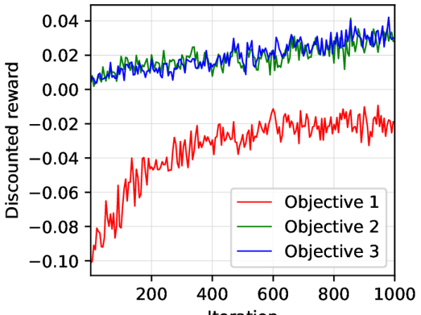
(a)

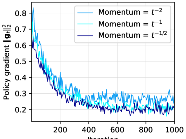
(b)

Figure 1: (a) Discounted rewards of three objectives with momentum $\eta_{t}=t^{-1}$; (b) Squared $\ell_{2}$-norm of policy gradients with different momentum coefficients.

Table 1: Comparison of our method with baseline methods.

Algorithm	Click$\uparrow$	Like$\uparrow$(e-2)	Follow$\uparrow$(e-4)	Comment$\uparrow$(e-3)	Forward$\uparrow$(e-3)	Dislike$\downarrow$(e-4)	WatchTime$\uparrow$
Behavior-Clone	$0.534$	$1.231$	$4.608$	$3.225^{*}$	$1.119^{*}$	$2.304$	$1.285$
TSCAC	$0.543^{*}$	$1.269$	$4.535$	$3.099$	$1.006$	$1.342$	$1.330^{*}$
	$1.49\%^{*}$	$3.09\%$	$-1.57\%$	$-3.92\%$	$-10.0\%$	$-41.8\%$	$3.43\%^{*}$
PDPG	$0.539$	$1.228$	$4.828^{*}$	$3.165$	$0.919$	$1.140^{*}$	$1.308$
	$1.02\%$	$-0.26\%$	$4.78\%^{*}$	$-1.86\%$	$-17.8\%$	$-50.5\%^{*}$	$1.74\%$
Ours	$0.539$	$1.287^{*}$	$4.800$	$3.151$	$0.897$	$1.428$	$1.282$
(fixed weights)	$0.98\%$	$4.54\%^{*}$	$4.19\%$	$-2.29\%$	$-19.8\%$	$-38.0\%$	$-0.27\%$
Ours	$0.541$	$\bm{1.312}$	$\bm{5.070}$	$\bm{3.266}$	$1.066$	$1.486$	$1.307$
	$1.30\%$	$\bm{6.57\%}$	$\bm{10.0\%}$	$\bm{1.27\%}$	$-4.76\%$	$-35.5\%$	$1.71\%$

1-b) Observations: In Fig. 1(a), with $\eta_{t}=t^{-1}$, all objectives are simultaneously improved, and the corresponding policy gradient in Fig. 1(b) converges. Also, as observed in Fig. 1(b), the policy gradient converges faster with a larger momentum coefficient $\eta_{t}$, e.g., when $\eta_{t}=t^{-1/2}$, $\|\mathbf{g}_{t}\|_{2}^{2}$ converges the fastest. This is consistent with our theoretical result in Theorem 5 that a larger $\eta_{t}$-value encourages the policy parameter update direction to follow more closely with the $\hat{\bm{\lambda}}_{t}^{*}$-weighted direction, which has a larger descent.

2) Real-World Data Experiments: 2-a) Dataset: Next, we use a real-world dataset collected from the recommendation logs of the video-sharing mobile app Kuaishou. The dataset includes user features and video features, as well as multiple reward signals, such as “Click,” “Like,” “Dislike,” “WatchTime,” etc. The statistic of the dataset is illustrated in Table 2. Specifically, a state corresponds to the event of a video watched by a user, and is represented by the concatenation of user feature and video feature; an action corresponds to a video recommended to a user.

Table 2: Data statistic. The reward data is imbalanced, with a density of over $98\%$ for the sum of Click and WatchTime.

State: $1218$  Action: 150
	Reward
	Click	Like	Follow	Comment	Forward	Dislike	WatchTime
Amount	$254940$	$5190$	$203$	$1438$	$349$	$213$	$199122$
Density	$55.25\%$	$1.125\%$	$0.044\%$	$0.312\%$	$0.076\%$	$0.046\%$	$43.15\%$

2-b) MORL Environment and Baselines: To our knowledge, $\mathsf{MOAC}$ is the first online actor-critic method for MORL. Thus, there is a lack of direct baseline methods. To have fair comparisons with other related (offline) MORL algorithms in the literature, we adapt $\mathsf{MOAC}$ to execute in an off-policy fashion by introducing a behavior policy, which generates actions following from the state-action samples in the dataset. We compare with the following methods.

• Behavior-Clone: A supervised behavior-cloning policy $\pi_{\beta}$ to mimic the recommendation policy in the dataset, which inputs the user state and outputs the video ID.

• PDPG (Chen et al., 2021a): A deterministic policy gradient based actor-critic method that learns Pareto-stationary policy by training networks with model parameters learned from a behavior policy. This method is the most related to ours, which shares the same goal of finding a Pareto-stationary point for all objectives.

• TSCAC (Cai et al., 2023): A two-stage constrained actor-critic approach that optimizes all individual objectives by a set of learned model weights with a focus on optimizing a main objective, while treating other objectives as constraints.

2-c) Evaluation: We adopt Normalised Capped Importance Sampling (NCIS) to evaluate the performances of the methods, which is a standard evaluation approach for off-policy reinforcement learning algorithms (Zou et al., 2019). NCIS score quantifies the optimality of a learned policy. A larger NCIS score implies a better policy for reward maximization. The definition of NCIS is provided in Section A.2.

2-d) Observations: The experiment results of baseline comparisons are summarized in Table 1. Note that our method and two baselines all start with the same critic and actor parameters initialized for policies that perform worse than Behavior-Clone. Thus, a negative improvement percentage regarding Behavior-Clone does not imply bad performance on a reward signal. Based on the result in Table 1, we have the following observations: (a) Our method outperforms PDPG in almost all objectives except “Dislike” and “WatchTime”. Despite the impact of imbalanced data, our method dominates PDPG in finding a Pareto-efficient policy for multi-objective optimization. (b) TSCAC outperforms our method in “Click”, “Dislike”, and “WatchTime”, while our method substantially outperforms TSCAC in all other four objectives. This is because TSCAC prioritizes WatchTime in optimization, while $\mathsf{MOAC}$ performs a balanced improvement in all objectives. (c) Compared to Behavior-Clone, $\mathsf{MOAC}$ achieves positive improvements in all objectives except “Forward,” while other baselines exhibit degraded performance in several objectives. TSCAC has negative improvements on “Follow”, “Comment”, and “Forward”; PDPG has negative improvements on “Like”, “Comment”, and “Forward”.

2-e) Ablation Studies: To show how $\mathsf{MOAC}$ performs on dynamically deciding a common gradient descent direction, we test another baseline with fixed weights that are initialized by $\mathsf{MOAC}$ in the first iteration. The results in Table 1 shows that $\mathsf{MOAC}$ outperforms the baseline in all the objectives except Dislike. This comparison indicates a significant performance improvement from the incorporation of momentum-based SMGD.

6 Conclusion and Future Work

In this paper, we investigated multi-objective reinforcement learning (MORL) problem by proposing the first MGDA-based actor-critic algorithm called $\mathsf{MOAC}$, which enjoys provable Pareto-stationary convergence and sample complexity guarantees. Future directions include a generalized model with linear reward signal or nonlinear value function approximation, multi-agent multi-objective reinforcement learning, and decentralized MORL.

Broader Impact

Real world applications of our actor-critic framework are broad among various fields. One typical example is the recommendation system, where our framework provides an architecture with theoretical guarantee. More applications include automatic driving, robotics, dynamic pricing, etc. In industry, related methods on MORL have been proposed and applied with different focuses in the last few decades, while our work focuses more on theoretical analysis. There can be potential societal consequences of our work, but none we feel must be specifically highlighted here.

Appendix

In this paper, we use $\|\cdot\|_{2},|\cdot|_{1},\|\cdot\|_{\infty}$, $\|\cdot\|_{F}$ to denote $\ell_{2}$, $\ell_{1}$, $\ell_{\infty}$, and Frobenius norms respectively, and $\|\cdot\|_{TV}$ for total variance norm. $\langle\cdot,\cdot\rangle$ denotes the inner product. Superscript $i$ in quantity $x$, i.e. $x^{i}$, denotes the $x$ quantity correspond to objective $i\in[M]$. $\lambda(\cdot)$ and $\sigma(\cdot)$ denote the eigenvalues and singular values of the corresponding matrix respectively. All vectors are assumed to be column vector, unless specified. $(\cdot)^{\top}$ is the transpose of an matrix or vector. We use $\mathbf{1}$ to denote all-1 vector with an appropriate dimension.

Appendix A Experimental Setup and Complementary Results

A.1 Synthetic Data

MOMDP Environment. We conduct synthetic simulations on two environments, described as follows:

Figure 2: Environment: Resource Gathering

Environment resource-gathering-v0 (Barrett & Narayanan, 2008):

• State space: $0$ (x coordinate of agent), $1$ (y coordinate of agent), $2$ (flag: gold collected), $3$ (flag: diamond collected)

• Action space: $0$ (up), $1$ (down), $2$ (left), $3$ (right)

• Reward space: obj 1: $-1$ (killed by enemy), obj 2: $+1$ (return home with gold), obj 3: $+1$ (return home with diamond)

• Starting state: The agent starts at the home position with no gold or diamond.

• Episode termination: When the agent returns home, or when the agent is killed by an enemy.

The FishWood environment is a simple MORL problem in which the agent controls a fisherman which can either fish or go collect wood. In this environment, fishing and collect wood are two conflicting objectives.

Figure 3: Environment: FishWood

Environment fishwood-v0 (Roijers et al., 2018):

• State space: $0$ (fishing), $1$ (in the woods)

• Action space: $0$ (go fishing), $1$ (go collect wood)

• Reward space: obj 1: $+1$ (if agent is in the woods, with woodproba probability),
  obj 2: $+1$ (if the agent is fishing, with fishproba probability)

• Starting state: Agent starts in the woods

• Episode termination: The episode ends after MAX_TS$=200$ steps

Simulation results and Observations.

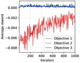
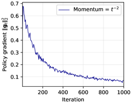
Figure 4: Resource Gathering environment. Average rewards of three objectives with momentum $\eta_{t}=t^{-2}$ (left), and squared $\ell_{2}$-norm of policy gradients (right).

Fig. 4 shows the average rewards of three objectives and corresponding policy gradient in Resource Gathering environment, we can observe that objective 2 and 3 are performing steady and objective 1 is optimized, with a converging policy gradient in the right hand side figure.

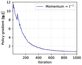
Figure 5: FishWood environment. Discounted rewards of two conflicting objectives with momentum $\eta_{t}=t^{-1}$ (left), and squared $\ell_{2}$-norm of policy gradients (right).

Fig. 5 shows the discounted rewards of two objectives and corresponding policy gradient in FishWood environment, the result shows that two discounted rewards are performing steady with a converging policy gradient. This is resulted from the fact that two objectives are conflicting, and optimizing any one will sacrifice the other.

A.2 Real-World Data

Environment and Setup. In the dataset, logs provided by the same user are concatenated to form a trajectory in one episode, and a batch of tuple $\{s_{t},a_{t},\bm{r}_{t},s_{t+1}\}$ are sampled at each iteration. For all the methods, we leverage ADAM to optimize the parameters. We only experiment on discounted total reward for fair comparison. For our method, we set the momentum coefficient of gradient weight by $\eta_{t}=1/t$ (without pre-specifying values, the gradient weights are initialized by the solution to a QP problem regarding the average gradients of the first batch of samples), and set the same gradient weight initialization for all the other methods.

Evaluation Metric. Specifically, NCIS score is defined as follows:

$$N(\pi)=\cfrac{\sum_{s,a\in D}w(s,a)r(s,a)}{\sum_{s,a\in D}w(s,a)},\quad w(s,a)=\min\bigg{\{}C,\cfrac{\pi(a\mid s)}{\pi_{\beta}(a\mid s)}\bigg{\}},$$

where $D$ is the dataset, $C$ is a positive constant, and $\pi_{\beta}$ is a behavior policy.

Appendix B Supporting Lemmas

Lemma 7.

Given a policy $\pi_{\bm{\theta}}$, for any objective $i\in[M]$, the TD fixed point for average reward setting $\mathbf{w}_{\bm{\theta}}^{i,*}$ is uniformly bounded, specifically, there exists constant $R_{\mathbf{w}}=4r_{\max}/\lambda_{A}>0$ such that

$$\|\mathbf{w}_{\bm{\theta}}^{i,*}\|\leq R_{\mathbf{w}},\forall i\in[M].$$

Proof.

$$\|\mathbf{w}^{i,*}_{\bm{\theta}}\|_{2} =\|-A_{\pi_{\bm{\theta}}}^{-1}\mathbf{b}^{i}_{\pi_{\bm{\theta}}}\|_{2}$$

$$=\|-\mathbb{E}_{s\sim d_{\bm{\theta}}(s),s^{\prime}\sim P(\cdot|s)}[(\bm{\phi}(s^{\prime})-\bm{\phi}(s))\bm{\phi}^{T}(s)]^{-1}\cdot\mathbb{E}_{s\sim d_{\bm{\theta}},a\sim\pi_{\bm{\theta}}}\left[\bm{\phi}(s)\left(r^{i}(s,a)-J^{i}(\bm{\theta})\right)\right]\|_{2}$$

$$\leq\|-\mathbb{E}_{s\sim d_{\bm{\theta}}(s),s^{\prime}\sim P(\cdot|s)}[(\bm{\phi}(s^{\prime})-\bm{\phi}(s))\bm{\phi}^{T}(s)]^{-1}\|_{2}\cdot\|\mathbb{E}_{s\sim d_{\bm{\theta}},a\sim\pi_{\bm{\theta}}}\left[\bm{\phi}(s)\left(r^{i}(s,a)-J^{i}(\bm{\theta})\right)\right]\|_{2}$$

$$\overset{\text{(i)}}{=}\cfrac{\|\mathbb{E}_{s\sim d_{\bm{\theta}},a\sim\pi_{\bm{\theta}}}\left[\bm{\phi}(s)\left(r^{i}(s,a)-J^{i}(\bm{\theta})\right)\right]\|_{2}}{{\sigma_{\min}}\left(\|-\mathbb{E}_{s\sim d_{\bm{\theta}}(s),s^{\prime}\sim P(\cdot|s)}[(\bm{\phi}(s^{\prime})-\bm{\phi}(s))\bm{\phi}^{T}(s)]\|_{2}\right)}$$

$$\overset{\text{(ii)}}{\leq}\cfrac{2\|\mathbb{E}_{s\sim d_{\bm{\theta}},a\sim\pi_{\bm{\theta}}}\left[\bm{\phi}(s)\left(r^{i}(s,a)-J^{i}(\bm{\theta})\right)\right]\|_{2}}{\lambda_{A}\left(-A_{\pi_{\bm{\theta}}}-A_{\pi_{\bm{\theta}}}^{\top}\right)}$$

$$\leq\cfrac{2\cdot\mathbb{E}_{s\sim d_{\bm{\theta}},a\sim\pi_{\bm{\theta}}}\left[\|\bm{\phi}(s)\|_{2}\cdot\left(|r^{i}(s,a)|+|J^{i}(\bm{\theta})|\right)\right]}{\lambda_{A}}$$

$$=\cfrac{4r_{\max}}{\lambda_{A}},$$

where (i) follows from the fact $\|A^{-1}\|=1/\sigma_{\min}(A)$, and (ii) follows from Bhatia (2013) (Proposition III 5.1). ∎

Lemma 8.

Given a policy $\pi_{\bm{\theta}}$ that maximizes discounted reward, for any objective $i\in[M]$, the optimal value function approximation parameter $\mathbf{w}_{\bm{\theta}}^{i,*}$ is uniformly bounded, specifically, there exists constant $R_{\mathbf{w}}=2r_{\max}/\lambda_{A}>0$ such that

$$\|\mathbf{w}_{\bm{\theta}}^{i,*}\|\leq R_{\mathbf{w}},\forall i\in[M].$$

Proof.

$$\|\mathbf{w}^{i,*}_{\bm{\theta}}\|_{2} =\|-A_{\pi_{\bm{\theta}}}^{-1}\mathbf{b}^{i}_{\pi_{\bm{\theta}}}\|_{2}$$

$$=\|-\mathbb{E}_{s\sim d_{\bm{\theta}}(s),s^{\prime}\sim P(\cdot|s)}\left[\left(\gamma\bm{\phi}(s^{\prime})-\bm{\phi}(s)\right)\bm{\phi}^{T}(s)\right]^{-1}\cdot\mathbb{E}_{s\sim d_{\bm{\theta}},a\sim\pi_{\bm{\theta}}}\left[r^{i}(s,a)\bm{\phi}(s)\right]\|_{2}$$

$$\leq\|-\mathbb{E}_{s\sim d_{\bm{\theta}}(s),s^{\prime}\sim P(\cdot|s)}\left[\left(\gamma\bm{\phi}(s^{\prime})-\bm{\phi}(s)\right)\bm{\phi}^{T}(s)\right]^{-1}\|_{2}\cdot\|\mathbb{E}_{s\sim d_{\bm{\theta}},a\sim\pi_{\bm{\theta}}}\left[r^{i}(s,a)\bm{\phi}(s)\right]\|_{2}$$

$$=\cfrac{\|\mathbb{E}_{s\sim d_{\bm{\theta}},a\sim\pi_{\bm{\theta}}}\left[r^{i}(s,a)\bm{\phi}(s)\right]\|_{2}}{\|-\mathbb{E}_{s\sim d_{\bm{\theta}}(s),s^{\prime}\sim P(\cdot|s)}\left[\left(\gamma\bm{\phi}(s^{\prime})-\bm{\phi}(s)\right)\bm{\phi}^{T}(s)\right]\|_{2}}$$

$$\leq\cfrac{2\|\mathbb{E}_{s\sim d_{\bm{\theta}},a\sim\pi_{\bm{\theta}}}\left[r^{i}(s,a)\bm{\phi}(s)\right]\|_{2}}{\lambda_{A}\left(-A_{\pi_{\bm{\theta}}}-A_{\pi_{\bm{\theta}}}^{\top}\right)}$$

$$\leq\cfrac{2\cdot\mathbb{E}_{s\sim d_{\bm{\theta}},a\sim\pi_{\bm{\theta}}}\left[\|\bm{\phi}(s)\|_{2}\cdot|r^{i}(s,a)|\right]}{\lambda_{A}}$$

$$=\cfrac{2r_{\max}}{\lambda_{A}}.$$

∎

Lemma 9.

(Hairi et al. (2022) Lemma 2) Let $\nu_{\bm{\theta}}$ denote the stationary distribution of the state-action pairs given policy $\pi_{\bm{\theta}}$, there exists constants $\kappa>0$ and $\rho\in(0,1)$ such that

$$\sup_{s\in\mathcal{S}}\|P(s_{t},a_{t}\mid s_{0}=s)-\nu_{\bm{\theta}}\|_{TV}\leq\kappa\rho^{t}.$$

Lemma 10.

(Hairi et al. (2022) Lemma 3) Suppose Assumption 2 holds. Given a policy $\pi_{\bm{\theta}}$, we have the following:

$$(-\mathbf{w}^{i,*}_{\bm{\theta}})^{\top}\mathbf{A}_{\pi_{\bm{\theta}}}(-\mathbf{w}^{i,*}_{\bm{\theta}})\leq-\lambda^{\prime}_{\mathbf{A}_{\pi_{\theta}}}\|\mathbf{w}^{i,*}_{\bm{\theta}}\|^{2}_{2}.$$

Lemma 11.

(Xu et al. (2020) Theorem 4) For any $i\in[M]$, consider mini-batched linear stochastic approximation on $\mathbf{A}_{\pi_{\bm{\theta}}}$, $\mathbf{b}_{\bm{\theta}}^{\prime i}$ (discounted setting), and $\mathbf{b}_{\bm{\theta}}^{i}$ (average setting), let $C_{\mathbf{A}}>\|\mathbf{A}_{\pi_{\bm{\theta}}}\|_{F}$ and $C_{\mathbf{b}}$ denote the upper bound for $\|\mathbf{b}_{\bm{\theta}}^{i}\|_{2}$ and $\|\mathbf{b}_{\bm{\theta}}^{\prime i}\|_{2}$, then by setting $\beta\leq\min\{{\lambda_{\mathbf{A}}\over 8C_{\mathbf{A}}^{2}},{4\over\lambda_{\mathbf{A}}}\}$ and $D\geq\left({2\over\lambda_{\mathbf{A}}}+2\beta\right){192C_{\mathbf{A}}^{2}[1+\rho(\kappa-1)]\over(1-\rho)\lambda_{\mathbf{A}}}$ and we have

$$\mathbb{E}\big{[}\|\mathbf{w}^{i}_{N}-\mathbf{w}^{i,*}_{\bm{\theta}}\|^{2}_{2}\big{]}\leq\left(1-\cfrac{\beta\lambda_{\mathbf{A}}}{8}\right)^{N}\cdot\|\mathbf{w}^{i}_{0}-\mathbf{w}^{i,*}_{\bm{\theta}}\|^{2}_{2}+\left({2\over\lambda_{\mathbf{A}}}+2\beta\right){192\left(C_{\mathbf{A}}^{2}R_{\mathbf{w}}^{2}+C_{\mathbf{b}}^{2}\right)[1+\rho(\kappa-1)]\over(1-\rho)\lambda_{\mathbf{A}}D}.$$

Further, setting $N\geq{8\over\beta\lambda_{\mathbf{A}}}\log\left(2\|\mathbf{w}^{i}_{0}-\mathbf{w}^{i,*}_{\bm{\theta}}\|^{2}_{2}/\epsilon\right)$ and $D\geq\left({2\over\lambda_{\mathbf{A}}}+2\beta\right){192\left(C_{\mathbf{A}}^{2}R_{\mathbf{w}}^{2}+C_{\mathbf{b}}^{2}\right)[1+\rho(\kappa-1)]\over\epsilon(1-\rho)\lambda_{\mathbf{A}}}$, we have $\mathbb{E}\big{[}\|\mathbf{w}^{i}_{N}-\mathbf{w}^{i,*}_{\bm{\theta}}\|^{2}_{2}\big{]}\leq\epsilon$ with total sample complexity $ND=\mathcal{O}\left(\epsilon^{-1}\log{(\epsilon^{-1})}\right)$.

Appendix C Proof of Theorem 3

Proof.

The results of Theorem 3 follows directly from Lemma 11, by setting $\mathbf{A}_{\pi_{\bm{\theta}}}:=\mathbb{E}_{s\sim d_{\bm{\theta}}(s),s^{\prime}\sim P(\cdot|s)}[(\bm{\phi}(s^{\prime})-\bm{\phi}(s))\bm{\phi}^{\top}(s)]$ and $\mathbf{b}^{i}_{\bm{\theta}}:=\mathbb{E}_{s\sim d_{\bm{\theta}},a\sim\pi_{\bm{\theta}}}\left[\left(r^{i}(s,a)-J^{i}(\bm{\theta})\right)\bm{\phi}(s)\right],\forall i\in[M]$ for the average reward setting, and by setting $\mathbf{A}_{\pi_{\theta}}:=\mathbb{E}_{s\sim d_{\theta}(s),s^{\prime}\sim P(\cdot|s)}\left[\left(\gamma\bm{\phi}(s^{\prime})-\bm{\phi}(s)\right)\bm{\phi}^{T}(s)\right]$ and $\mathbf{b}^{\prime i}_{\bm{\theta}}:=\mathbb{E}_{s\sim d_{\bm{\theta}},a\sim\pi_{\bm{\theta}}}\left[r^{i}(s,a)\bm{\phi}(s)\right],\forall i\in[M]$ for the discounted reward setting.

For clarity, we present Theorem 3 with some terms simplified as constants, where $C_{1}=\|\mathbf{w}^{i}_{0}-\mathbf{w}^{i,*}_{\bm{\theta}}\|^{2}_{2}$, $C_{2}=[1+(\kappa-1)\rho]/(1-\rho)$, and $C_{3}=192\left(C_{\mathbf{A}}^{2}R_{\mathbf{w}}^{2}+C_{\mathbf{b}}^{2}\right)$. ∎

Appendix D Proof of Theorem 5

For any given $\bm{\theta}$, we denote the gradient matrix to be

$$\nabla_{\bm{\theta}}\bm{J}(\bm{\theta})=\left[\begin{matrix}\nabla_{\bm{\theta}}J^{1}(\bm{\theta})&\nabla_{\bm{\theta}}J^{2}(\bm{\theta})&\cdots&\nabla_{\bm{\theta}}J^{M}(\bm{\theta})\end{matrix}\right]\in\mathbb{R}^{d_{1}\times M}.$$

Proof.

We first present the proof in average reward setting, then we show how to obtain the results in discounted reward setting. Given $\bm{\theta}\in\mathbb{R}^{d_{1}}$, $\mathbf{w}\in\mathbb{R}^{d_{2}}$, $t\geq 0$ and $i\in[M]$, by Lipschitzness in Assumption 3, we have

$$J^{i}(\bm{\theta}_{t+1})\geq J^{i}(\bm{\theta}_{t})+\left\langle\nabla_{\bm{\theta}}J^{i}(\bm{\theta}_{t}),\bm{\theta}_{t+1}-\bm{\theta}_{t}\right\rangle-\cfrac{L_{J}}{2}\|\bm{\theta}_{t+1}-\bm{\theta}_{t}\|^{2}$$ (12)

Note that $J^{i}(\bm{\theta})$ is an expected value taken, where the expectation is taken over steady-state distribution induced by policy $\pi_{\bm{\theta}}$. We use $\bm{\lambda}^{*}_{t}$ to denote the QP solution for using $\{\nabla_{\bm{\theta}}J^{i}(\bm{\theta}_{t})\}_{i\in[M]}$, which again is a set of expected vectors. In comparison, $\bm{\lambda}_{t}$ is the QP solution with momentum for using $\{\mathbf{g}_{t}^{i}\}_{i\in[M]}$ as in Algorithm 2.

Taking $\bm{\lambda}_{t}$ weighted summation over Eq. (12), we have

$$\bm{\lambda}_{t}^{\top}\bm{J}(\bm{\theta}_{t+1}) \geq\bm{\lambda}_{t}^{\top}\bm{J}(\bm{\theta}_{t})+\left\langle\nabla_{\bm{\theta}}\bm{J}(\bm{\theta}_{t})\bm{\lambda}_{t},\bm{\theta}_{t+1}-\bm{\theta}_{t}\right\rangle-\cfrac{L_{J}}{2}\|\bm{\theta}_{t+1}-\bm{\theta}_{t}\|_{2}^{2}$$

$$=\bm{\lambda}_{t}^{\top}\bm{J}(\bm{\theta}_{t})+\alpha\left\langle\nabla_{\bm{\theta}}\bm{J}(\bm{\theta}_{t})\bm{\lambda}_{t},\sum_{j=1}^{M}\lambda_{t}^{j}\cdot\mathbf{g}_{t}^{j}\right\rangle-\cfrac{\alpha^{2}L_{J}}{2}\|\mathbf{g}_{t}\|_{2}^{2}$$

$$=\bm{\lambda}_{t}^{\top}\bm{J}(\bm{\theta}_{t})+\alpha\left\langle\nabla_{\bm{\theta}}\bm{J}(\bm{\theta}_{t})\bm{\lambda}_{t},\sum_{j=1}^{M}\lambda_{t}^{j}\cdot\left(\mathbf{g}_{t}^{j}-\nabla_{\bm{\theta}}J^{j}(\bm{\theta}_{t})+\nabla_{\bm{\theta}}J^{j}(\bm{\theta}_{t})\right)\right\rangle-\cfrac{\alpha^{2}L_{J}}{2}\|\mathbf{g}_{t}\|_{2}^{2}$$

$$=\bm{\lambda}_{t}^{\top}\bm{J}(\bm{\theta}_{t})+\alpha\left\langle\nabla_{\bm{\theta}}\bm{J}(\bm{\theta}_{t})\bm{\lambda}_{t},\sum_{j=1}^{M}\lambda_{t}^{j}\nabla_{\bm{\theta}}J^{j}(\bm{\theta}_{t})\right\rangle$$

$$\hskip 13.0pt+\alpha\left\langle\nabla_{\bm{\theta}}\bm{J}(\bm{\theta}_{t})\bm{\lambda}_{t},\sum_{j=1}^{M}\lambda_{t}^{j}\cdot\left(\mathbf{g}_{t}^{j}-\nabla_{\bm{\theta}}J^{j}(\bm{\theta}_{t})\right)\right\rangle-\cfrac{\alpha^{2}L_{J}}{2}\|\mathbf{g}_{t}\|_{2}^{2}$$

$$=\bm{\lambda}_{t}^{\top}\bm{J}(\bm{\theta}_{t})+\alpha\left\|\nabla_{\bm{\theta}}\bm{J}(\bm{\theta}_{t})\bm{\lambda}_{t}\right\|^{2}_{2}+\alpha\left\langle\nabla_{\bm{\theta}}\bm{J}(\bm{\theta}_{t})\bm{\lambda}_{t},\sum_{j=1}^{M}\lambda_{t}^{j}\cdot\left(\mathbf{g}_{t}^{j}-\nabla_{\bm{\theta}}J^{j}(\bm{\theta}_{t})\right)\right\rangle-\cfrac{\alpha^{2}L_{J}}{2}\|\mathbf{g}_{t}\|_{2}^{2}$$

$$\overset{\text{(i)}}{\geq}\bm{\lambda}_{t}^{\top}\bm{J}(\bm{\theta}_{t})+\cfrac{\alpha}{2}\left\|\nabla_{\bm{\theta}}\bm{J}(\bm{\theta}_{t})\bm{\lambda}_{t}\right\|^{2}_{2}-\cfrac{\alpha}{2}\left\|\sum_{j=1}^{M}\lambda_{t}^{j}\cdot\left(\nabla_{\bm{\theta}}J^{j}(\bm{\theta}_{t})-\mathbf{g}_{t}^{j}\right)\right\|^{2}_{2}-\cfrac{\alpha^{2}L_{J}}{2}\|\mathbf{g}_{t}\|_{2}^{2}$$

$$=\bm{\lambda}_{t}^{\top}\bm{J}(\bm{\theta}_{t})+\cfrac{\alpha}{2}\left\|\nabla_{\bm{\theta}}\bm{J}(\bm{\theta}_{t})\bm{\lambda}_{t}\right\|^{2}_{2}-\cfrac{\alpha}{2}\left\|\sum_{j=1}^{M}\lambda_{t}^{j}\cdot\left(\nabla_{\bm{\theta}}J^{j}(\bm{\theta}_{t})-\mathbf{g}_{t}^{j}\right)\right\|^{2}_{2}$$

$$\hskip 13.0pt-\cfrac{\alpha^{2}L_{J}}{2}\left\|\sum_{j=1}^{M}\lambda_{t}^{j}\cdot\left(\mathbf{g}_{t}^{j}-\nabla_{\bm{\theta}}J^{j}(\bm{\theta}_{t})+\nabla_{\bm{\theta}}J^{j}(\bm{\theta}_{t})\right)\right\|_{2}^{2}$$

$$\overset{\text{(ii)}}{\geq}\bm{\lambda}_{t}^{\top}\bm{J}(\bm{\theta}_{t})+\left(\cfrac{\alpha}{2}-\alpha^{2}L_{J}\right)\left\|\nabla_{\bm{\theta}}\bm{J}(\bm{\theta}_{t})\bm{\lambda}_{t}\right\|^{2}_{2}-\left(\cfrac{\alpha}{2}+\alpha^{2}L_{J}\right)\left\|\sum_{j=1}^{M}\lambda_{t}^{j}\cdot\left(\nabla_{\bm{\theta}}J^{j}(\bm{\theta}_{t})-\mathbf{g}_{t}^{j}\right)\right\|^{2}_{2},$$ (13)

where inequality (i) follows because

$$\left\langle\nabla_{\bm{\theta}}\bm{J}(\bm{\theta}_{t})\bm{\lambda}_{t},\sum_{j=1}^{M}\lambda_{t}^{j}\cdot\left(\mathbf{g}_{t}^{j}-\nabla_{\bm{\theta}}J^{j}(\bm{\theta}_{t})\right)\right\rangle\geq-\cfrac{1}{2}\left\|\nabla_{\bm{\theta}}\bm{J}(\bm{\theta}_{t})\bm{\lambda}_{t}\right\|^{2}_{2}-\cfrac{1}{2}\left\|\sum_{j=1}^{M}\lambda_{t}^{j}\cdot\left(\nabla_{\bm{\theta}}J^{j}(\bm{\theta}_{t})-\mathbf{g}_{t}^{j}\right)\right\|^{2}_{2},$$

and inequality (ii) follows because

$$\left\|\sum_{j=1}^{M}\lambda_{t}^{j}\cdot\left(\mathbf{g}_{t}^{j}-\nabla_{\bm{\theta}}J^{j}(\bm{\theta}_{t})+\nabla_{\bm{\theta}}J^{j}(\bm{\theta}_{t})\right)\right\|_{2}^{2}\leq 2\left\|\nabla_{\bm{\theta}}\bm{J}(\bm{\theta}_{t})\bm{\lambda}_{t}\right\|^{2}_{2}+2\left\|\sum_{j=1}^{M}\lambda_{t}^{j}\cdot\left(\nabla_{\bm{\theta}}J^{j}(\bm{\theta}_{t})-\mathbf{g}_{t}^{j}\right)\right\|^{2}_{2}.$$

Taking expectation on both sides of Eq. (13) and conditioning on $\mathcal{F}_{t}$, we have

$$\mathbb{E}\left[\left\|\nabla_{\bm{\theta}}\bm{J}(\bm{\theta}_{t})\bm{\lambda}_{t}\right\|^{2}_{2}\mid\mathcal{F}_{t}\right]\leq\cfrac{2\left(\mathbb{E}\left[\bm{\lambda}_{t}^{\top}\bm{J}(\bm{\theta}_{t+1})|\mathcal{F}_{t}\right]-\bm{\lambda}_{t}^{\top}\bm{J}(\bm{\theta}_{t})\right)}{\alpha-2\alpha^{2}L_{J}}+\cfrac{\alpha+2\alpha^{2}L_{J}}{\alpha-2\alpha^{2}L_{J}}\mathbb{E}\left[\left\|\sum_{j=1}^{M}\lambda_{t}^{j}\left(\nabla_{\bm{\theta}}J^{j}(\bm{\theta}_{t})-\mathbf{g}_{t}^{j}\right)\right\|^{2}_{2}\bigg{|}\mathcal{F}_{t}\right].$$

By the definitions of $\bm{\lambda}^{*}_{t}$ and $\bm{\lambda}_{t}$, for any time $t$, we have

$$\mathbb{E}\left[\left\|\nabla_{\bm{\theta}}\bm{J}(\bm{\theta}_{t})\bm{\lambda}_{t}^{*}\right\|^{2}_{2}\mid\mathcal{F}_{t}\right]\leq\mathbb{E}\left[\left\|\nabla_{\bm{\theta}}\bm{J}(\bm{\theta}_{t})\bm{\lambda}_{t}\right\|^{2}_{2}\mid\mathcal{F}_{t}\right].$$

Thus

$$\mathbb{E}\left[\left\|\nabla_{\bm{\theta}}\bm{J}(\bm{\theta}_{t})\bm{\lambda}_{t}^{*}\right\|^{2}_{2}\mid\mathcal{F}_{t}\right]\leq\cfrac{2\left(\mathbb{E}\left[\bm{\lambda}_{t}^{\top}\bm{J}(\bm{\theta}_{t+1})|\mathcal{F}_{t}\right]-\bm{\lambda}_{t}^{\top}\bm{J}(\bm{\theta}_{t})\right)}{\alpha-2\alpha^{2}L_{J}}+\cfrac{\alpha+2\alpha^{2}L_{J}}{\alpha-2\alpha^{2}L_{J}}\mathbb{E}\left[\left\|\sum_{j=1}^{M}\lambda_{t}^{j}\left(\nabla_{\bm{\theta}}J^{j}(\bm{\theta}_{t})-\mathbf{g}_{t}^{j}\right)\right\|^{2}_{2}\bigg{|}\mathcal{F}_{t}\right].$$ (14)

D.1 For the 2nd Term on RHS of Eq. (14)

Define a notation: $\Delta^{j}_{\bm{\theta}_{t},\mathbf{w}_{t}^{*}}=\mathbb{E}_{d_{\bm{\theta}}}\left[\mathbb{E}_{P_{\bm{\theta}}}\left[\delta_{t,l}^{j}(\mathbf{w}_{t}^{j,*})\mid(a_{t,l},s_{t,l})\right]\cdot\bm{\psi}^{\bm{\theta}}_{t,l}\right]$. We first bound the last term on the right hand side of Eq. (14) as follows:

$$\hskip 13.0pt\mathbb{E}\left[\left\|\sum_{j=1}^{M}\lambda_{t}^{j}\left(\nabla_{\bm{\theta}}J^{j}(\bm{\theta}_{t})-\mathbf{g}_{t}^{j}\right)\right\|^{2}_{2}\bigg{|}\mathcal{F}_{t}\right]$$

$$\leq\mathbb{E}\left[\left(\sum_{j=1}^{M}\lambda_{t}^{j}\left\|\nabla_{\bm{\theta}}J^{j}(\bm{\theta}_{t})-\mathbf{g}_{t}^{j}\right\|_{2}\right)^{2}\bigg{|}\mathcal{F}_{t}\right]$$

$$\leq\mathbb{E}\left[\left(\sum_{j=1}^{M}\lambda_{t}^{j}\left(\left\|\nabla_{\bm{\theta}}J^{j}(\bm{\theta}_{t})-\Delta^{j}_{\bm{\theta}_{t},\mathbf{w}_{t}^{*}}\right\|_{2}+\left\|\Delta^{j}_{\bm{\theta}_{t},\mathbf{w}_{t}^{*}}-\mathbf{g}^{j}_{\bm{\theta}_{t}^{*}}\right\|_{2}+\left\|\mathbf{g}^{j}_{\bm{\theta}_{t}^{*}}-\mathbf{g}_{t}^{j}\right\|_{2}\right)\right)^{2}\bigg{|}\mathcal{F}_{t}\right]$$

$$\leq 3\mathbb{E}\left[\left(\sum_{j=1}^{M}\lambda_{t}^{j}\left\|\nabla_{\bm{\theta}}J^{j}(\bm{\theta}_{t})-\Delta^{j}_{\bm{\theta}_{t},\mathbf{w}_{t}^{*}}\right\|_{2}\right)^{2}\bigg{|}\mathcal{F}_{t}\right]+3\mathbb{E}\left[\left(\sum_{j=1}^{M}\lambda_{t}^{j}\left\|\mathbf{g}^{j}_{\bm{\theta}_{t}^{*}}-\mathbf{g}_{t}^{j}\right\|_{2}\right)^{2}\bigg{|}\mathcal{F}_{t}\right]$$

$$\hskip 13.0pt+3\mathbb{E}\left[\left(\sum_{j=1}^{M}\lambda_{t}^{j}\cdot\left\|\Delta^{j}_{\bm{\theta}_{t},\mathbf{w}_{t}^{*}}-\mathbf{g}^{j}_{\bm{\theta}_{t}^{*}}\right\|_{2}\right)^{2}\bigg{|}\mathcal{F}_{t}\right],$$ (15)

where

$$\left\|\nabla_{\bm{\theta}}J^{j}(\bm{\theta}_{t})-\Delta^{j}_{\bm{\theta}_{t},\mathbf{w}_{t}^{*}}\right\|^{2}_{2} =\left\|\mathbb{E}_{d_{\bm{\theta}}}\left[\mathbb{E}_{P_{\bm{\theta}}}\left[\delta_{t,l}^{j}\mid(a_{t,l},s_{t,l})\right]\cdot\bm{\psi}^{\bm{\theta}}_{t,l}\right]-\mathbb{E}_{d_{\bm{\theta}}}\left[\mathbb{E}_{P_{\bm{\theta}}}\left[\delta_{t,l}^{j}(\mathbf{w}_{t}^{j,*})\mid(a_{t,l},s_{t,l})\right]\cdot\bm{\psi}^{\bm{\theta}}_{t,l}\right]\right\|^{2}_{2}$$

$$=\left\|\mathbb{E}_{d_{\bm{\theta}}}\left[\left(\mathbb{E}_{P_{\bm{\theta}}}\left[\delta_{t,l}^{j}\mid(a_{t,l},s_{t,l})\right]-\mathbb{E}_{P_{\bm{\theta}}}\left[\delta_{t,l}^{j}(\mathbf{w}_{t}^{j,*})\mid(a_{t,l},s_{t,l})\right]\right)\cdot\bm{\psi}^{\bm{\theta}}_{t,l}\right]\right\|^{2}_{2}$$

$$\leq\mathbb{E}_{d_{\bm{\theta}}}\left[\left\|\left(\mathbb{E}_{P_{\bm{\theta}}}\left[\delta_{t,l}^{j}\mid(a_{t,l},s_{t,l})\right]-\mathbb{E}_{P_{\bm{\theta}}}\left[\delta_{t,l}^{j}(\mathbf{w}_{t}^{j,*})\mid(a_{t,l},s_{t,l})\right]\right)\cdot\bm{\psi}^{\bm{\theta}}_{t,l}\right\|^{2}_{2}\right]$$

$$\leq\mathbb{E}_{d_{\bm{\theta}}}\left[\left|\mathbb{E}_{P_{\bm{\theta}}}\left[\delta_{t,l}^{j}\mid(a_{t,l},s_{t,l})\right]-\mathbb{E}_{P_{\bm{\theta}}}\left[\delta_{t,l}^{j}(\mathbf{w}_{t}^{j,*})\mid(a_{t,l},s_{t,l})\right]\right|^{2}\right]$$

$$=\mathbb{E}_{d_{\bm{\theta}}}\left[\left|\mathbb{E}\left[V_{\bm{\theta}}^{j}(s_{t,l+1})-V_{\bm{\theta}}^{j}(s_{t,l+1};\mathbf{w}_{t}^{j,*})\mid(a_{t,l},s_{t,l})\right]+V_{\bm{\theta}}^{j}(s_{t,l})-V_{\bm{\theta}}^{j}(s_{t,l};\mathbf{w}_{t}^{j,*})\right|^{2}\right]$$

$$\leq 4\zeta_{\text{approx}}.$$

We note that $\delta^{j}_{t,l}$ denotes the TD error for objective $j\in[M]$ using the ground truth value functions. We also remark that the above inequality holds for all $j\in[M]$. As a result, for the first term on the RHS of Eq. (15), we have

$$\mathbb{E}\left[\left(\sum_{j=1}^{M}\lambda_{t}^{j}\left\|\nabla_{\bm{\theta}}J^{j}(\bm{\theta}_{t})-\Delta^{j}_{\bm{\theta}_{t},\mathbf{w}_{t}^{*}}\right\|_{2}\right)^{2}\bigg{|}\mathcal{F}_{t}\right]\leq\mathbb{E}\left[\left(\sum_{j=1}^{M}\lambda_{t}^{j}2\sqrt{\zeta_{\text{approx}}}\right)^{2}\bigg{|}\mathcal{F}_{t}\right]=4\zeta_{\text{approx}}$$

Furthermore, we have

$$\left\|\mathbf{g}^{j}_{\bm{\theta}_{t}^{*}}-\mathbf{g}_{t}^{j}\right\|_{2} =\left\|\cfrac{1}{B}\sum_{l=0}^{B-1}\left(\delta_{t,l}^{j}(\mathbf{w}^{j}_{t})-\delta_{t,l}^{j}(\mathbf{w}^{j,*}_{t})\right)\cdot\bm{\psi}^{\bm{\theta}}_{t,l}\right\|_{2}$$

$$=\left\|\cfrac{1}{B}\sum_{l=0}^{B-1}\left(\bm{\phi}(s_{t,l+1})-\bm{\phi}(s_{t,l})\right)^{\top}\left(\mathbf{w}^{j}_{t}-\mathbf{w}^{j,*}_{t}\right)\cdot\bm{\psi}^{\bm{\theta}}_{t,l}\right\|_{2}$$

$$\leq\left\|\cfrac{1}{B}\sum_{l=0}^{B-1}\left(\bm{\phi}(s_{t,l+1})-\bm{\phi}(s_{t,l})\right)^{\top}\left(\mathbf{w}^{j}_{t}-\mathbf{w}^{j,*}_{t}\right)\right\|_{2}$$

$$\leq\max_{l\in\{0,\ldots,B-1\}}\left\|\left(\bm{\phi}(s_{t,l+1})-\bm{\phi}(s_{t,l})\right)^{\top}\left(\mathbf{w}^{j}_{t}-\mathbf{w}^{j,*}_{t}\right)\right\|_{2}$$

$$\leq 2\cdot\left\|\mathbf{w}^{j}_{t}-\mathbf{w}^{j,*}_{t}\right\|_{2}.$$

As a result, for the second term on the RHS of Eq. (15), we have

$$\mathbb{E}\left[\left(\sum_{j=1}^{M}\lambda_{t}^{j}\left\|\mathbf{g}^{j}_{\bm{\theta}_{t}^{*}}-\mathbf{g}_{t}^{j}\right\|_{2}\right)^{2}\bigg{|}\mathcal{F}_{t}\right]\leq\mathbb{E}\left[\left(\sum_{j=1}^{M}\lambda_{t}^{j}2\left\|\mathbf{w}^{j}_{t}-\mathbf{w}^{j,*}_{t}\right\|_{2}\right)^{2}\bigg{|}\mathcal{F}_{t}\right]\leq 4\max_{i\in[M]}\mathbb{E}\left[\left\|\mathbf{w}^{i}_{t}-\mathbf{w}^{i,*}_{t}\right\|^{2}_{2}\bigg{|}\mathcal{F}_{t}\right].$$ (16)

Similarly, for the last term in Eq. (15), we have

$$\mathbb{E}\bigg{[}\bigg{(}\sum_{j=1}^{M}\lambda_{t}^{j}\cdot\left\|\Delta^{j}_{\bm{\theta}_{t},\mathbf{w}_{t}^{*}}-\mathbf{g}^{j}_{\bm{\theta}_{t}^{*}}\right\|_{2}\bigg{)}^{2}\bigg{|}\mathcal{F}_{t}\bigg{]}\leq\max_{i\in[M]}\mathbb{E}\bigg{[}\bigg{(}\sum_{j=1}^{M}\lambda_{t}^{j}\cdot\left\|\Delta^{i}_{\bm{\theta}_{t},\mathbf{w}_{t}^{*}}-\mathbf{g}^{i}_{\bm{\theta}_{t}^{*}}\right\|_{2}\bigg{)}^{2}\bigg{|}\mathcal{F}_{t}\bigg{]}=\max_{i\in[M]}\mathbb{E}\left[\left\|\Delta^{i}_{\bm{\theta}_{t},\mathbf{w}_{t}^{*}}-\mathbf{g}^{i}_{\bm{\theta}_{t}^{*}}\right\|^{2}_{2}\bigg{|}\mathcal{F}_{t}\right].$$

In addition, for any $j\in[M]$, we have

$$\hskip 13.0pt\mathbb{E}\left[\left\|\Delta^{j}_{\bm{\theta}_{t},\mathbf{w}_{t}^{*}}-\mathbf{g}^{j}_{\bm{\theta}_{t}^{*}}\right\|_{2}^{2}\bigg{|}\mathcal{F}_{t}\right]$$

$$=\mathbb{E}\left[\left\|\cfrac{1}{B}\sum_{l=0}^{B-1}\delta^{j}_{t,l}(\mathbf{w}^{j,*}_{t})\cdot\bm{\psi}^{\bm{\theta}}_{t,l}-\Delta^{j}_{\bm{\theta}_{t},\mathbf{w}_{t}^{*}}\right\|_{2}^{2}\bigg{|}\mathcal{F}_{t}\right]$$

$$=\mathbb{E}\left[\left\langle\cfrac{1}{B}\sum_{l_{1}=0}^{B-1}\delta^{j}_{t,l_{1}}(\mathbf{w}^{j,*}_{t})\cdot\bm{\psi}^{\bm{\theta}}_{t,l_{1}}-\Delta^{j}_{\bm{\theta}_{t},\mathbf{w}_{t}^{*}},\cfrac{1}{B}\sum_{l_{2}=0}^{B-1}\delta^{j}_{t,l_{2}}(\mathbf{w}^{j,*}_{t})\cdot\bm{\psi}^{\bm{\theta}}_{t,l_{2}}-\Delta^{j}_{\bm{\theta}_{t},\mathbf{w}_{t}^{*}}\right\rangle\bigg{|}\mathcal{F}_{t}\right]$$

$$=\mathbb{E}\left[\cfrac{1}{B^{2}}\sum_{l=0}^{B-1}\left\|\delta^{j}_{t,l}(\mathbf{w}^{j,*}_{t})\bm{\psi}^{\bm{\theta}}_{t,l}-\Delta^{j}_{\bm{\theta}_{t},\mathbf{w}_{t}^{*}}\right\|_{2}^{2}+\cfrac{1}{B^{2}}\sum_{l_{1}\neq l_{2}}\left\langle\delta^{j}_{t,l_{1}}(\mathbf{w}^{j,*}_{t})\cdot\bm{\psi}^{\bm{\theta}}_{t,l_{1}}-\Delta^{j}_{\bm{\theta}_{t},\mathbf{w}_{t}^{*}},\delta^{j}_{t,l_{2}}(\mathbf{w}^{j,*}_{t})\cdot\bm{\psi}^{\bm{\theta}}_{t,l_{2}}-\Delta^{j}_{\bm{\theta}_{t},\mathbf{w}_{t}^{*}}\right\rangle\bigg{|}\mathcal{F}_{t}\right]$$

$$\overset{\text{(i)}}{\leq}\cfrac{16}{B}\left(r_{\max}+R_{\mathbf{w}}\right)^{2}+\cfrac{1}{B^{2}}\sum_{l_{1}\neq l_{2}}\mathbb{E}\left[\left\langle\delta^{j}_{t,l_{1}}(\mathbf{w}^{j,*}_{t})\cdot\bm{\psi}^{\bm{\theta}}_{t,l_{1}}-\Delta^{j}_{\bm{\theta}_{t},\mathbf{w}_{t}^{*}},\delta^{j}_{t,l_{2}}(\mathbf{w}^{j,*}_{t})\cdot\bm{\psi}^{\bm{\theta}}_{t,l_{2}}-\Delta^{j}_{\bm{\theta}_{t},\mathbf{w}_{t}^{*}}\right\rangle\bigg{|}\mathcal{F}_{t}\right]$$

$$=\cfrac{16}{B}(r_{\max}+R_{\mathbf{w}})^{2}+\cfrac{2}{B^{2}}\sum_{l_{1}<l_{2}}\mathbb{E}\left[\left\langle\delta^{j}_{t,l_{1}}(\mathbf{w}^{j,*}_{t})\cdot\bm{\psi}^{\bm{\theta}}_{t,l_{1}}-\Delta^{j}_{\bm{\theta}_{t},\mathbf{w}_{t}^{*}},\delta^{j}_{t,l_{2}}(\mathbf{w}^{j,*}_{t})\cdot\bm{\psi}^{\bm{\theta}}_{t,l_{2}}-\Delta^{j}_{\bm{\theta}_{t},\mathbf{w}_{t}^{*}}\right\rangle\bigg{|}\mathcal{F}_{t}\right]$$

$$=\cfrac{16}{B}(r_{\max}+R_{\mathbf{w}})^{2}+\cfrac{2}{B^{2}}\sum_{l_{1}<l_{2}}\mathbb{E}\left[\left\langle\delta^{j}_{t,l_{1}}(\mathbf{w}^{j,*}_{t})\cdot\bm{\psi}^{\bm{\theta}}_{t,l_{1}}-\Delta^{j}_{\bm{\theta}_{t},\mathbf{w}_{t}^{*}},\mathbb{E}\left[\delta^{j}_{t,l_{2}}(\mathbf{w}^{j,*}_{t})\cdot\bm{\psi}^{\bm{\theta}}_{t,l_{2}}\big{|}\mathcal{F}_{t,l_{1}}\right]-\Delta^{j}_{\bm{\theta}_{t},\mathbf{w}_{t}^{*}}\right\rangle\bigg{|}\mathcal{F}_{t}\right]$$

$$\leq\cfrac{16}{B}(r_{\max}+R_{\mathbf{w}})^{2}+\cfrac{2}{B^{2}}\sum_{l_{1}<l_{2}}\mathbb{E}\left[\left\|\delta^{j}_{t,l_{1}}(\mathbf{w}^{j,*}_{t})\cdot\bm{\psi}^{\bm{\theta}}_{t,l_{1}}-\Delta^{j}_{\bm{\theta}_{t},\mathbf{w}_{t}^{*}}\right\|_{2}\cdot\left\|\mathbb{E}\left[\delta^{j}_{t,l_{2}}(\mathbf{w}^{j,*}_{t})\cdot\bm{\psi}^{\bm{\theta}}_{t,l_{2}}\big{|}\mathcal{F}_{t,l_{1}}\right]-\Delta^{j}_{\bm{\theta}_{t},\mathbf{w}_{t}^{*}}\right\|_{2}\bigg{|}\mathcal{F}_{t}\right]$$

$$\leq\cfrac{16}{B}(r_{\max}+R_{\mathbf{w}})^{2}+\cfrac{2}{B^{2}}\sum_{l_{1}<l_{2}}4\left(r_{\max}+R_{\mathbf{w}}\right)\mathbb{E}\left[\left\|\mathbb{E}\left[\delta^{j}_{t,l_{2}}(\mathbf{w}^{j,*}_{t})\cdot\bm{\psi}^{\bm{\theta}}_{t,l_{2}}\big{|}\mathcal{F}_{t,l_{1}}\right]-\Delta^{j}_{\bm{\theta}_{t},\mathbf{w}_{t}^{*}}\right\|_{2}\bigg{|}\mathcal{F}_{t}\right]$$

$$\overset{\text{(ii)}}{\leq}\cfrac{16}{B}(r_{\max}+R_{\mathbf{w}})^{2}+\cfrac{2}{B^{2}}\sum_{l_{1}<l_{2}}16(r_{\max}+R_{\mathbf{w}})^{2}\kappa\rho^{l_{2}-l_{1}},$$

where (i) follows from the facts that

$$|\delta^{j}_{t,l}(\mathbf{w}^{j,*}_{t})| =|r^{j}_{t,l+1}-\mu^{j}_{t,l}+\bm{\phi}(s_{t,l+1})^{\top}\mathbf{w}^{j}_{t}-\bm{\phi}(s_{t,l})^{\top}\mathbf{w}^{j}_{t}|_{1}$$

$$\leq|r^{j}_{t,l+1}|+|\mu^{j}_{t,l}|+\|\bm{\phi}(s_{t,l+1})-\bm{\phi}(s_{t,l})\|_{2}\cdot\|\mathbf{w}^{j}_{t}\|_{2}$$

$$\leq 2r_{\max}+2R_{\mathbf{w}},$$

thus, $\|\delta^{j}_{t,l}(\mathbf{w}^{j,*}_{t})\bm{\psi}^{\bm{\theta}}_{t,l}\|_{2}\leq 2r_{\max}+2R_{\mathbf{w}}$, and $\Delta^{j}_{\bm{\theta}_{t},\mathbf{w}_{t}^{*}}=\mathbb{E}_{d_{\bm{\theta}}}\left[\mathbb{E}_{P_{\bm{\theta}}}\left[\delta_{t,l}^{j}(\mathbf{w}_{t}^{j,*})\mid(a_{t,l},s_{t,l})\right]\cdot\bm{\psi}^{\bm{\theta}}_{t,l}\right]\leq 2r_{\max}+2R_{\mathbf{w}}$, and (ii) follows from

$$\hskip 13.0pt\left\|\mathbb{E}\left[\delta^{j}_{t,l_{2}}(\mathbf{w}^{j,*}_{t})\cdot\bm{\psi}^{\bm{\theta}}_{t,l_{2}}\big{|}\mathcal{F}_{t,l_{1}}\right]-\Delta^{j}_{\bm{\theta}_{t},\mathbf{w}_{t}^{*}}\right\|_{2}$$

$$=\left\|\mathbb{E}\left[\delta^{j}_{t,l_{2}}(\mathbf{w}^{j,*}_{t})\cdot\bm{\psi}^{\bm{\theta}}_{t,l_{2}}\big{|}\mathcal{F}_{t,l_{1}}\right]-\mathbb{E}_{d_{\bm{\theta}}}\left[\mathbb{E}_{P_{\bm{\theta}}}\left[\delta_{t,l}^{j}(\mathbf{w}_{t}^{j,*})\mid(s_{t,l},a_{t,l})\right]\cdot\bm{\psi}^{\bm{\theta}}_{t,l}\right]\right\|_{2}$$

$$=\bigg{\|}\sum_{(s_{t,l_{2}},a_{t,l_{2}})}\mathbb{E}_{P_{\bm{\theta}}}\left[\delta_{t,l_{2}}^{j}(\mathbf{w}_{t}^{j,*})\mid(s_{t,l_{2}},a_{t,l_{2}})\right]\cdot\bm{\psi}^{\bm{\theta}}_{t,l}\cdot P(s_{t,l_{2}},a_{t,l_{2}}\mid\mathcal{F}_{t,l_{1}})$$

$$\hskip 13.0pt-\sum_{(s_{t,l},a_{t,l})}\mathbb{E}_{P_{\bm{\theta}}}\left[\delta_{t,l}^{j}(\mathbf{w}_{t}^{j,*})\mid(s_{t,l},a_{t,l})\right]\cdot\bm{\psi}^{\bm{\theta}}_{t,l}\cdot\nu_{\bm{\theta}_{t}}(s_{t,l},a_{t,l})\bigg{\|}_{2}$$

$$\leq\sum_{(s_{t,l},a_{t,l})}\left\|\mathbb{E}_{P_{\bm{\theta}}}\left[\delta_{t,l}^{j}(\mathbf{w}_{t}^{j,*})\mid(s_{t,l},a_{t,l})\right]\cdot\bm{\psi}^{\bm{\theta}}_{t,l}\right\|_{2}\cdot\left|P^{l_{2}-l_{1}}(s_{t,l},a_{t,l}\mid\mathcal{F}_{t,l_{1}})-\nu_{\bm{\theta}_{t}}(s_{t,l},a_{t,l})\right|$$

$$\overset{\text{(i)}}{\leq}4(r_{\max}+R_{\mathbf{w}})\cdot\left\|P^{l_{2}-l_{1}}(s,a\mid\mathcal{F}_{t,l_{1}})-\nu_{\bm{\theta}_{t}}(s,a)\right\|_{TV}$$

$$\leq 4(r_{\max}+R_{\mathbf{w}})\kappa\rho^{l_{2}-l_{1}},$$

where (i) follows from Lemma 9.

Therefore, for the last term in Eq. (15), we have

$$\mathbb{E}\left[\left(\sum_{j=1}^{M}\lambda_{t}^{j}\cdot\left\|\Delta^{j}_{\bm{\theta}_{t},\mathbf{w}_{t}^{*}}-\mathbf{g}^{j}_{\bm{\theta}_{t}^{*}}\right\|_{2}\right)^{2}\bigg{|}\mathcal{F}_{t}\right] \leq\cfrac{16}{B}(r_{\max}+R_{\mathbf{w}})^{2}+\cfrac{32}{B^{2}}\sum_{l_{1}<l_{2}}(r_{\max}+R_{\mathbf{w}})^{2}\kappa\rho^{l_{2}-l_{1}}$$

$$\leq\cfrac{16}{B}(r_{\max}+R_{\mathbf{w}})^{2}+\cfrac{32}{B^{2}}(r_{\max}+R_{\mathbf{w}})^{2}\cfrac{2\kappa\rho B}{1-\rho}$$

$$=\cfrac{16(r_{\max}+R_{\mathbf{w}})^{2}(1-\rho+4\kappa\rho)}{(1-\rho)B}.$$ (17)

Substituting Eqs. (D.1), (16), (17) into Eq. (15) yields the expected gradient bias as follows

$$\hskip 13.0pt\mathbb{E}\left[\left\|\sum_{j=1}^{M}\lambda_{t}^{j}\left(\nabla_{\bm{\theta}}J^{j}(\bm{\theta}_{t})-\mathbf{g}_{t}^{j}\right)\right\|^{2}_{2}\bigg{|}\mathcal{F}_{t}\right]$$

$$\hskip 13.0pt\leq 12\zeta_{\text{approx}}+12\mathbb{E}\left[\left\|w^{i}_{t}-w^{i,*}_{t}\right\|^{2}_{2}\bigg{|}\mathcal{F}_{t}\right]+\cfrac{48(r_{\max}+R_{\mathbf{w}})^{2}(1-\rho+4\kappa\rho)}{(1-\rho)B}.$$ (18)

Substituting Eq. (18) into Eq. (14), letting $\alpha=\cfrac{1}{3L_{J}}$, and taking expectation of $\mathcal{F}_{t}$ yields

$$\mathbb{E}\left[\left\|\nabla_{\bm{\theta}}\bm{J}(\bm{\theta}_{t})\bm{\lambda}_{t}^{*}\right\|^{2}_{2}\right] \leq 18L_{J}\left(\mathbb{E}\left[\bm{\lambda}_{t}^{\top}\bm{J}(\bm{\theta}_{t+1})\right]-\bm{\lambda}_{t}^{\top}\bm{J}(\bm{\theta}_{t})\right)+12{\zeta_{\text{approx}}}+12\max_{j\in[M]}\mathbb{E}\left[\left\|\mathbf{w}^{j}_{t}-\mathbf{w}^{j,*}_{t}\right\|_{2}^{2}\right]$$

$$\hskip 13.0pt+\cfrac{48(r_{\max}+R_{\mathbf{w}})^{2}(1-\rho+4\kappa\rho)}{(1-\rho)B}.$$ (19)

D.2 For the 1st Term on RHS of Eq. (14)

Let $\hat{T}$ denote a random variable that takes value uniformly random among $\{1,\ldots,T\}$, then taking average of Eq. (19) over $T$ and we have

$$\mathbb{E}\left[\left\|\nabla_{\bm{\theta}}\bm{J}(\bm{\theta}_{\hat{T}})\bm{\lambda}_{\hat{T}}^{*}\right\|^{2}_{2}\right] =\cfrac{1}{T}\sum_{t=1}^{T}\mathbb{E}\left[\left\|\nabla_{\bm{\theta}}\bm{J}(\bm{\theta}_{t})\bm{\lambda}_{t}^{*}\right\|^{2}_{2}\right]$$

$$\leq\cfrac{18L_{J}}{T}\sum_{t=1}^{T}\left(\mathbb{E}\left[\bm{\lambda}_{t}^{\top}\bm{J}(\bm{\theta}_{t+1})\right]-\bm{\lambda}_{t}^{\top}\bm{J}(\bm{\theta}_{t})\right)+\cfrac{12}{T}\sum_{t=1}^{T}\max_{j\in[M]}\mathbb{E}\left[\left\|\mathbf{w}^{j}_{t}-\mathbf{w}^{j,*}_{t}\right\|_{2}^{2}\right]$$

$$\hskip 13.0pt+\cfrac{48(r_{\max}+R_{\mathbf{w}})^{2}(1-\rho+4\kappa\rho)}{(1-\rho)B}+12\zeta_{\text{approx}}.$$

Specifically,

$$\sum_{t=1}^{T}\left(\mathbb{E}\left[\bm{\lambda}_{t}^{\top}\bm{J}(\bm{\theta}_{t+1})\right]-\bm{\lambda}_{t}^{\top}\bm{J}(\bm{\theta}_{t})\right) =\mathbb{E}\left[\sum_{t=1}^{T-1}(-\bm{\lambda}_{t+1}+\bm{\lambda}_{t})^{\top}\bm{J}(\bm{\theta}_{t+1})-\bm{\lambda}^{\top}_{1}\bm{J}(\bm{\theta}_{1})+\bm{\lambda}^{\top}_{T}\bm{J}(\bm{\theta}_{T+1})\right]$$

$$\overset{\text{(i)}}{\leq}\mathbb{E}\left[\sum_{t=1}^{T-1}|\bm{\lambda}_{t+1}-\bm{\lambda}_{t}|_{1}\|\bm{J}(\bm{\theta}_{t+1})\|_{\infty}+\|\bm{\lambda}_{T}\|_{1}\|\bm{J}(\bm{\theta}_{T+1})\|_{\infty}\right]$$

$$\leq r_{\max}+r_{\max}\sum_{t=1}^{T}\mathbb{E}\left[|\bm{\lambda}_{t+1}-\bm{\lambda}_{t}|_{1}\right]$$

$$=r_{\max}\left(1+\sum_{t=1}^{T}\eta_{t}\cdot\mathbb{E}\left[|\hat{\bm{\lambda}}_{t+1}^{*}-\bm{\lambda}_{t}|_{1}\right]\right)$$

$$\leq r_{\max}\left(1+\sum_{t=1}^{T}2\eta_{t}\right),$$

where (i) follows from Hölder’s Inequality since $1/1+1/\infty=1$. This facilitates the analysis to be $M$-independent in the telescoping process. Then, we have

$$\mathbb{E}\left[\left\|\nabla_{\bm{\theta}}\bm{J}(\bm{\theta}_{\hat{T}})\bm{\lambda}_{\hat{T}}\right\|^{2}_{2}\right] \leq\cfrac{18L_{J}r_{\max}}{T}\left(1+\sum_{t=1}^{T}2\eta_{t}\right)+\cfrac{12}{T}\sum_{t=1}^{T}\max_{j\in[M]}\mathbb{E}\left[\left\|\mathbf{w}^{j}_{t}-\mathbf{w}^{j,*}_{t}\right\|_{2}^{2}\right]$$

$$\hskip 13.0pt+\cfrac{48(r_{\max}+R_{\mathbf{w}})^{2}(1-\rho+4\kappa\rho)}{(1-\rho)B}+12\zeta_{\text{approx}}.$$

D.3 Final Result for Average Reward Setting

Recalling that $\alpha=\cfrac{1}{3L_{J}}$ and by letting $T\geq\cfrac{18L_{J}r_{\max}}{\epsilon}\cdot\max\{1,\sum_{t=1}^{T}2\eta_{t}\}$, $\mathbb{E}\left[\left\|\mathbf{w}^{j}_{t}-\mathbf{w}^{j,*}_{t}\right\|_{2}^{2}\right]\leq\cfrac{\epsilon}{12}$ for any objective $j\in[M]$, and $B\geq\cfrac{48(r_{\max}+R_{\mathbf{w}})^{2}(1-\rho+4\kappa\rho)}{\epsilon}$ yields

$$\mathbb{E}\left[\left\|\bm{\lambda}_{\hat{T}}^{\top}\nabla_{\bm{\theta}}\bm{J}(\bm{\theta}_{\hat{T}})\right\|^{2}_{2}\right]\leq\epsilon+60\zeta_{\text{approx}},$$

with a total sample complexity given by

$$(B+ND)T=\mathcal{O}\left(\left(\cfrac{1}{\epsilon}+\cfrac{1}{\epsilon}\log\cfrac{1}{\epsilon}\right)\cfrac{1}{\epsilon}\right)=\mathcal{O}\left(\cfrac{1}{\epsilon^{2}}\log\cfrac{1}{\epsilon}\right).$$

D.4 Final Result for Discounted Reward Setting

Similar to the proof in average reward setting, we have

$$\mathbb{E}\left[\left\|\nabla_{\bm{\theta}}\bm{J}(\bm{\theta}_{t})\bm{\lambda}_{t}^{*}\right\|^{2}_{2}\mid\mathcal{F}_{t}\right]\leq\cfrac{2\left(\mathbb{E}\left[\bm{\lambda}_{t}^{\top}\bm{J}(\bm{\theta}_{t+1})|\mathcal{F}_{t}\right]-\bm{\lambda}_{t}^{\top}\bm{J}(\bm{\theta}_{t})\right)}{\alpha-2\alpha^{2}L_{J}}+\cfrac{\alpha+2\alpha^{2}L_{J}}{\alpha-2\alpha^{2}L_{J}}\mathbb{E}\left[\left\|\sum_{j=1}^{M}\lambda_{t}^{j}\left(\nabla_{\bm{\theta}}J^{j}(\bm{\theta}_{t})-\mathbf{g}_{t}^{j}\right)\right\|^{2}_{2}\bigg{|}\mathcal{F}_{t}\right],$$ (20)

where the last term on the right hand side is bounded by

$$\hskip 13.0pt\mathbb{E}\left[\left\|\sum_{j=1}^{M}\lambda_{t}^{j}\left(\nabla_{\bm{\theta}}J^{j}(\bm{\theta}_{t})-\mathbf{g}_{t}^{j}\right)\right\|^{2}_{2}\bigg{|}\mathcal{F}_{t}\right]$$

$$\leq 3\mathbb{E}\left[\left(\sum_{j=1}^{M}\lambda_{t}^{j}\left\|\nabla_{\bm{\theta}}J^{j}(\bm{\theta}_{t})-\Delta^{j}_{\bm{\theta}_{t},\mathbf{w}_{t}^{*}}\right\|_{2}\right)^{2}\bigg{|}\mathcal{F}_{t}\right]$$

$$\hskip 13.0pt+3\mathbb{E}\left[\left(\sum_{j=1}^{M}\lambda_{t}^{j}\left\|\mathbf{g}^{j}_{\bm{\theta}_{t}^{*}}-\mathbf{g}_{t}^{j}\right\|_{2}\right)^{2}\bigg{|}\mathcal{F}_{t}\right]+3\mathbb{E}\left[\left(\sum_{j=1}^{M}\lambda_{t}^{j}\cdot\left\|\Delta^{j}_{\bm{\theta}_{t},\mathbf{w}_{t}^{*}}-\mathbf{g}^{j}_{\bm{\theta}_{t}^{*}}\right\|_{2}\right)^{2}\bigg{|}\mathcal{F}_{t}\right].$$ (21)

Considering the discounted factor $\gamma$, we have

$$\left\|\nabla_{\bm{\theta}}J^{j}(\bm{\theta}_{t})-\Delta^{j}_{\bm{\theta}_{t},\mathbf{w}_{t}^{*}}\right\|_{2}\leq 2\sqrt{\zeta_{\text{approx}}},$$ (22)

and

$$\left\|\mathbf{g}^{j}_{\bm{\theta}_{t}^{*}}-\mathbf{g}_{t}^{j}\right\|_{2}\leq 2\cdot\left\|\mathbf{w}^{j}_{t}-\mathbf{w}^{j,*}_{t}\right\|_{2}.$$ (23)

For the last term in Eq. (21), we have

$$\mathbb{E}\left[\left|\sum_{j=1}^{M}\lambda_{t}^{j}\cdot\left\|\Delta^{j}_{\bm{\theta}_{t},\mathbf{w}_{t}^{*}}-\mathbf{g}^{j}_{\bm{\theta}_{t}^{*}}\right\|_{2}\right|^{2}\bigg{|}\mathcal{F}_{t}\right]\leq\cfrac{4(r_{\max}+2R_{\mathbf{w}})^{2}(1-\rho+4\kappa\rho)}{(1-\rho)B},$$ (24)

since the facts

$$|\delta^{j}_{t,l}(\mathbf{w}^{j,*}_{t})| =|r^{j}_{t,l+1}+\gamma\bm{\phi}(s_{t,l+1})^{\top}\mathbf{w}^{j}_{t}-\bm{\phi}(s_{t,l})^{\top}\mathbf{w}^{j}_{t}|_{1}$$

$$\leq|r^{j}_{t,l+1}|+\|\gamma\bm{\phi}(s_{t,l+1})-\bm{\phi}(s_{t,l})\|_{2}\cdot\|\mathbf{w}^{j}_{t}\|_{2}$$

$$\leq r_{\max}+2R_{\mathbf{w}},$$

thus, $\|\delta^{j}_{t,l}(\mathbf{w}^{j,*}_{t})\bm{\psi}^{\bm{\theta}}_{t,l}\|_{2}\leq r_{\max}+2R_{\mathbf{w}}$, and $\Delta^{j}_{\bm{\theta}_{t},\mathbf{w}_{t}^{*}}=\mathbb{E}_{d_{\bm{\theta}}}\left[\mathbb{E}_{P_{\bm{\theta}}}\left[\delta_{t,l}^{j}(\mathbf{w}_{t}^{j,*})\mid(a_{t,l},s_{t,l})\right]\cdot\bm{\psi}^{\bm{\theta}}_{t,l}\right]\leq r_{\max}+2R_{\mathbf{w}}$.

Substituting Eqs. (22), (23), (24) into Eq. (21), we have

$$\mathbb{E}\left[\left\|\sum_{j=1}^{M}\lambda_{t}^{j}\left(\nabla_{\bm{\theta}}J^{j}(\bm{\theta}_{t})-\mathbf{g}_{t}^{j}\right)\right\|^{2}_{2}\bigg{|}\mathcal{F}_{t}\right]\leq 12{\zeta_{\text{approx}}}+12\max_{j\in[M]}\mathbb{E}\left[\left\|\mathbf{w}^{j}_{t}-\mathbf{w}^{j,*}_{t}\right\|_{2}^{2}\bigg{|}\mathcal{F}_{t}\right]+\cfrac{12(r_{\max}+2R_{\mathbf{w}})^{2}(1-\rho+4\kappa\rho)}{(1-\rho)B}.$$ (25)

Substituting Eq. (25) into Eq. (20), letting $\alpha=\cfrac{1}{3L_{J}}$, taking expectation of $\mathcal{F}_{t}$, and taking average of Eq. (20) over $T$ yields

$$\mathbb{E}\left[\left\|\nabla_{\bm{\theta}}\bm{J}(\bm{\theta}_{\hat{T}})\bm{\lambda}_{\hat{T}}^{*}\right\|^{2}_{2}\right] =\cfrac{1}{T}\sum_{t=1}^{T}\mathbb{E}\left[\left\|\nabla_{\bm{\theta}}\bm{J}(\bm{\theta}_{t})\bm{\lambda}_{t}^{*}\right\|^{2}_{2}\right]$$

$$\leq\cfrac{18L_{J}}{T}\sum_{t=1}^{T}\left(\mathbb{E}\left[\bm{\lambda}_{t}^{\top}\bm{J}(\bm{\theta}_{t+1})\right]-\bm{\lambda}_{t}^{\top}\bm{J}(\bm{\theta}_{t})\right)+\cfrac{12}{T}\sum_{t=1}^{T}\max_{j\in[M]}\mathbb{E}\left[\left\|\mathbf{w}^{j}_{t}-\mathbf{w}^{j,*}_{t}\right\|_{2}^{2}\right]$$

$$\hskip 13.0pt+\cfrac{4(r_{\max}+2R_{\mathbf{w}})^{2}(1-\rho+4\kappa\rho)}{(1-\rho)B}+12\zeta_{\text{approx}},$$

where

$$\sum_{t=1}^{T}\left(\mathbb{E}\left[\bm{\lambda}_{t}^{\top}\bm{J}(\bm{\theta}_{t+1})\right]-\bm{\lambda}_{t}^{\top}\bm{J}(\bm{\theta}_{t})\right) =\mathbb{E}\left[\sum_{t=1}^{T-1}(-\bm{\lambda}_{t+1}+\bm{\lambda}_{t})^{\top}\bm{J}(\bm{\theta}_{t+1})-\bm{\lambda}^{\top}_{1}\bm{J}(\bm{\theta}_{1})+\bm{\lambda}^{\top}_{T}\bm{J}(\bm{\theta}_{T+1})\right]$$

$$\leq\mathbb{E}\left[\sum_{t=1}^{T-1}|\bm{\lambda}_{t+1}-\bm{\lambda}_{t}|_{1}\|\bm{J}(\bm{\theta}_{t+1})\|_{\infty}+|\bm{\lambda}_{T}|_{1}\|\bm{J}(\bm{\theta}_{T+1})\|_{\infty}\right]$$

$$\leq\sum_{t=1}^{T-1}\left[\eta_{t}\mathbb{E}\left[|\bm{\lambda}_{t}-\hat{\bm{\lambda}}_{t}|_{1}\right]\frac{r_{\max}}{1-\|\bm{\gamma}\|_{\infty}}\right]+\cfrac{r_{\max}}{1-\|\bm{\gamma}\|_{\infty}}$$

$$\leq\cfrac{r_{\max}}{1-\|\bm{\gamma}\|_{\infty}}(1+\sum_{t=1}^{T}2\eta_{t}).$$

Then, we have

$$\mathbb{E}\left[\left\|\nabla_{\bm{\theta}}\bm{J}(\bm{\theta}_{\hat{T}})\bm{\lambda}_{\hat{T}}\right\|^{2}_{2}\right] \leq\cfrac{18L_{J}r_{\max}}{T(1-\|\bm{\gamma}\|_{\infty})}(1+2\sum_{t=1}^{T}\eta_{t})+\cfrac{12}{T}\sum_{t=1}^{T}\max_{j\in[M]}\mathbb{E}\left[\left\|\mathbf{w}^{j}_{t}-\mathbf{w}^{j,*}_{t}\right\|_{2}^{2}\right]$$

$$\hskip 13.0pt+\cfrac{12(r_{\max}+2R_{\mathbf{w}})^{2}(1-\rho+4\kappa\rho)}{(1-\rho)B}+12\zeta_{\text{approx}}.$$

By letting $T\geq\cfrac{18L_{J}r_{\max}}{\epsilon(1-\|\bm{\gamma}\|_{\infty})}\cdot\max\{1,\sum_{t=1}^{T}2\eta_{t}\}$, $\mathbb{E}\left[\left\|\mathbf{w}^{j}_{t}-\mathbf{w}^{j,*}_{t}\right\|_{2}^{2}\right]\leq\cfrac{\epsilon}{12}$ for any objective $j\in[M]$, and $B\geq\cfrac{12(r_{\max}+2R_{\mathbf{w}})^{2}(1-\rho+4\kappa\rho)}{\epsilon}$ yields

$$\mathbb{E}\left[\left\|\bm{\lambda}_{\hat{T}}^{\top}\nabla_{\bm{\theta}}\bm{J}(\bm{\theta}_{\hat{T}})\right\|^{2}_{2}\right]\leq\epsilon+12\zeta_{\text{approx}},$$

with total sample complexity given by

$$(B+ND)T=\mathcal{O}\left(\left(\cfrac{1}{\epsilon}+\cfrac{1}{\epsilon}\log\cfrac{1}{\epsilon}\right)\cfrac{1}{\epsilon}\right)=\mathcal{O}\left(\cfrac{1}{\epsilon^{2}}\log\cfrac{1}{\epsilon}\right).$$

∎

References

• Abels et al. (2019) Abels, A., Roijers, D., Lenaerts, T., Nowé, A., and Steckelmacher, D. Dynamic weights in multi-objective deep reinforcement learning. In International conference on machine learning, pp.  11–20. PMLR, 2019.
• Alegre et al. (2022) Alegre, L. N., Felten, F., Talbi, E.-G., Danoy, G., Nowé, A., Bazzan, A. L. C., and da Silva, B. C. MO-Gym: A library of multi-objective reinforcement learning environments. In Proceedings of the 34th Benelux Conference on Artificial Intelligence BNAIC/Benelearn 2022, 2022.
• Barrett & Narayanan (2008) Barrett, L. and Narayanan, S. Learning all optimal policies with multiple criteria. In Proceedings of the 25th international conference on Machine learning, pp.  41–47, 2008.
• Bhatia (2013) Bhatia, R. Matrix analysis, volume 169. Springer Science & Business Media, 2013.
• Bhatnagar et al. (2009) Bhatnagar, S., Sutton, R. S., Ghavamzadeh, M., and Lee, M. Natural actor–critic algorithms. Automatica, 45(11):2471–2482, 2009.
• Cai et al. (2023) Cai, Q., Xue, Z., Zhang, C., Xue, W., Liu, S., Zhan, R., Wang, X., Zuo, T., Xie, W., Zheng, D., et al. Two-stage constrained actor-critic for short video recommendation. In Proceedings of the ACM Web Conference 2023, pp.  865–875, 2023.
• Chen et al. (2021a) Chen, X., Du, Y., Xia, L., and Wang, J. Reinforcement recommendation with user multi-aspect preference. In Proceedings of the Web Conference 2021, pp.  425–435, 2021a.
• Chen et al. (2021b) Chen, Z., Zhou, Y., Chen, R., and Zou, S. Sample and communication-efficient decentralized actor-critic algorithms with finite-time analysis. arXiv preprint arXiv:2109.03699, 2021b.
• Danilova et al. (2022) Danilova, M., Dvurechensky, P., Gasnikov, A., Gorbunov, E., Guminov, S., Kamzolov, D., and Shibaev, I. Recent theoretical advances in non-convex optimization. In High-Dimensional Optimization and Probability: With a View Towards Data Science, pp.  79–163. Springer, 2022.
• Désidéri (2012) Désidéri, J.-A. Multiple-gradient descent algorithm (mgda) for multiobjective optimization. Comptes Rendus Mathematique, 350(5-6):313–318, 2012.
• Doan et al. (2019) Doan, T., Maguluri, S., and Romberg, J. Finite-time analysis of distributed td (0) with linear function approximation on multi-agent reinforcement learning. In International Conference on Machine Learning, pp.  1626–1635. PMLR, 2019.
• Doan et al. (2018) Doan, T. T., Maguluri, S. T., and Romberg, J. Distributed stochastic approximation for solving network optimization problems under random quantization. arXiv preprint arXiv:1810.11568, 2018.
• Fernando et al. (2022) Fernando, H. D., Shen, H., Liu, M., Chaudhury, S., Murugesan, K., and Chen, T. Mitigating gradient bias in multi-objective learning: A provably convergent approach. In The Eleventh International Conference on Learning Representations, 2022.
• Fliege et al. (2019) Fliege, J., Vaz, A. I. F., and Vicente, L. N. Complexity of gradient descent for multiobjective optimization. Optimization Methods and Software, 34(5):949–959, 2019.
• Gábor et al. (1998) Gábor, Z., Kalmár, Z., and Szepesvári, C. Multi-criteria reinforcement learning. In ICML, volume 98, pp.  197–205, 1998.
• Ge et al. (2022) Ge, Y., Zhao, X., Yu, L., Paul, S., Hu, D., Hsieh, C.-C., and Zhang, Y. Toward pareto efficient fairness-utility trade-off in recommendation through reinforcement learning. In Proceedings of the fifteenth ACM international conference on web search and data mining, pp.  316–324, 2022.
• Grondman et al. (2012) Grondman, I., Busoniu, L., Lopes, G. A., and Babuska, R. A survey of actor-critic reinforcement learning: Standard and natural policy gradients. IEEE Transactions on Systems, Man, and Cybernetics, Part C (Applications and Reviews), 42(6):1291–1307, 2012.
• Guo et al. (2021) Guo, X., Hu, A., and Zhang, J. Theoretical guarantees of fictitious discount algorithms for episodic reinforcement learning and global convergence of policy gradient methods. arXiv preprint arXiv:2109.06362, 2021.
• Hairi et al. (2022) Hairi, F., Liu, J., and Lu, S. Finite-time convergence and sample complexity of multi-agent actor-critic reinforcement learning with average reward. In International Conference on Learning Representations, 2022.
• Konda & Tsitsiklis (1999) Konda, V. and Tsitsiklis, J. Actor-critic algorithms. Advances in neural information processing systems, 12, 1999.
• Kumar et al. (2019) Kumar, H., Koppel, A., and Ribeiro, A. On the sample complexity of actor-critic for reinforcement learning. In Conference on Neural Information Processing Systems (NeurIPS), 2019.
• Lakshminarayanan & Szepesvari (2018) Lakshminarayanan, C. and Szepesvari, C. Linear stochastic approximation: How far does constant step-size and iterate averaging go? In International Conference on Artificial Intelligence and Statistics, pp.  1347–1355. PMLR, 2018.
• Levin & Peres (2017) Levin, D. A. and Peres, Y. Markov chains and mixing times, volume 107. American Mathematical Soc., 2017.
• Levine et al. (2016) Levine, S., Finn, C., Darrell, T., and Abbeel, P. End-to-end training of deep visuomotor policies. The Journal of Machine Learning Research, 17(1):1334–1373, 2016.
• Liu & Vicente (2021) Liu, S. and Vicente, L. N. The stochastic multi-gradient algorithm for multi-objective optimization and its application to supervised machine learning. Annals of Operations Research, pp.  1–30, 2021.
• Mao et al. (2016) Mao, H., Alizadeh, M., Menache, I., and Kandula, S. Resource management with deep reinforcement learning. In the 15th ACM Workshop on Hot Topics in Networks, pp.  50–56, 2016.
• Miettinen (1999) Miettinen, K. Nonlinear multiobjective optimization, volume 12. Springer Science & Business Media, 1999.
• Petersen et al. (2019) Petersen, B. K., Yang, J., Grathwohl, W. S., Cockrell, C., Santiago, C., An, G., and Faissol, D. M. Deep reinforcement learning and simulation as a path toward precision medicine. Journal of Computational Biology, 26(6):597–604, 2019.
• Qiu et al. (2021) Qiu, S., Yang, Z., Ye, J., and Wang, Z. On finite-time convergence of actor-critic algorithm. IEEE Journal on Selected Areas in Information Theory, 2(2):652–664, 2021.
• Raghu et al. (2017a) Raghu, A., Komorowski, M., Ahmed, I., Celi, L., Szolovits, P., and Ghassemi, M. Deep reinforcement learning for sepsis treatment. arXiv preprint arXiv:1711.09602, 2017a.
• Raghu et al. (2017b) Raghu, A., Komorowski, M., Celi, L. A., Szolovits, P., and Ghassemi, M. Continuous state-space models for optimal sepsis treatment: a deep reinforcement learning approach. In Machine Learning for Healthcare Conference, pp.  147–163. PMLR, 2017b.
• Roijers et al. (2018) Roijers, D. M., Steckelmacher, D., and Nowé, A. Multi-objective reinforcement learning for the expected utility of the return. In Proceedings of the Adaptive and Learning Agents workshop at FAIM, volume 2018, 2018.
• Sener & Koltun (2018) Sener, O. and Koltun, V. Multi-task learning as multi-objective optimization. Advances in neural information processing systems, 31, 2018.
• Srikant & Ying (2019) Srikant, R. and Ying, L. Finite-time error bounds for linear stochastic approximation andtd learning. In Conference on Learning Theory, pp.  2803–2830. PMLR, 2019.
• Stamenkovic et al. (2022) Stamenkovic, D., Karatzoglou, A., Arapakis, I., Xin, X., and Katevas, K. Choosing the best of both worlds: Diverse and novel recommendations through multi-objective reinforcement learning. In Proceedings of the Fifteenth ACM International Conference on Web Search and Data Mining, pp.  957–965, 2022.
• Sutton & Barto (2018) Sutton, R. S. and Barto, A. G. Reinforcement learning: An introduction. MIT press, 2018.
• Sutton et al. (1999) Sutton, R. S., McAllester, D. A., Singh, S. P., Mansour, Y., et al. Policy gradient methods for reinforcement learning with function approximation. In NIPs, volume 99, pp.  1057–1063. Citeseer, 1999.
• Theocharous et al. (2015) Theocharous, G., Thomas, P. S., and Ghavamzadeh, M. Personalized ad recommendation systems for life-time value optimization with guarantees. In the 24th International Joint Conference on Artificial Intelligence, 2015.
• Tsitsiklis & Van Roy (1999) Tsitsiklis, J. N. and Van Roy, B. Average cost temporal-difference learning. Automatica, 35(11):1799–1808, 1999.
• Van Moffaert & Nowé (2014) Van Moffaert, K. and Nowé, A. Multi-objective reinforcement learning using sets of pareto dominating policies. The Journal of Machine Learning Research, 15(1):3483–3512, 2014.
• Wei et al. (2022) Wei, H., Liu, X., and Ying, L. Triple-q: A model-free algorithm for constrained reinforcement learning with sublinear regret and zero constraint violation. In Camps-Valls, G., Ruiz, F. J. R., and Valera, I. (eds.), Proceedings of The 25th International Conference on Artificial Intelligence and Statistics, volume 151 of Proceedings of Machine Learning Research, pp.  3274–3307. PMLR, 28–30 Mar 2022. URL https://proceedings.mlr.press/v151/wei22a.html.
• Wen et al. (2023) Wen, W., Liu, K.-H., Fedorov, I., Zhang, X., Yin, H., Chu, W., Hassani, K., Sun, M., Liu, J., Wang, X., et al. Rankitect: Ranking architecture search battling world-class engineers at meta scale. arXiv preprint arXiv:2311.08430, 2023.
• Xu et al. (2020) Xu, T., Wang, Z., and Liang, Y. Improving sample complexity bounds for (natural) actor-critic algorithms. arXiv preprint arXiv:2004.12956, 2020.
• Yang et al. (2024) Yang, H., Liu, Z., Liu, J., Dong, C., and Momma, M. Federated multi-objective learning. 2024.
• Yang et al. (2019) Yang, R., Sun, X., and Narasimhan, K. A generalized algorithm for multi-objective reinforcement learning and policy adaptation. Advances in neural information processing systems, 32, 2019.
• Zerbinati et al. (2011) Zerbinati, A., Desideri, J.-A., and Duvigneau, R. Comparison between MGDA and PAES for multi-objective optimization. PhD thesis, INRIA, 2011.
• Zhang et al. (2018) Zhang, K., Yang, Z., Liu, H., Zhang, T., and Basar, T. Fully decentralized multi-agent reinforcement learning with networked agents. In International Conference on Machine Learning, pp.  5872–5881. PMLR, 2018.
• Zhang et al. (2021) Zhang, X., Liu, Z., Liu, J., Zhu, Z., and Lu, S. Taming communication and sample complexities in decentralized policy evaluation for cooperative multi-agent reinforcement learning. In Advances Neural Information Processing Systems (NeurIPS), Virtual Event, December 2021.
• Zhou et al. (2022) Zhou, S., Zhang, W., Jiang, J., Zhong, W., Gu, J., and Zhu, W. On the convergence of stochastic multi-objective gradient manipulation and beyond. Advances in Neural Information Processing Systems, 35:38103–38115, 2022.
• Zou et al. (2019) Zou, L., Xia, L., Ding, Z., Song, J., Liu, W., and Yin, D. Reinforcement learning to optimize long-term user engagement in recommender systems. In Proceedings of the 25th ACM SIGKDD International Conference on Knowledge Discovery & Data Mining, pp.  2810–2818, 2019.