A hydrodynamic model of capillary flow in an axially symmetric tube with a non-slowly-varying cross section and a boundary slip
Abstract
The capillary flow of a Newtonian and incompressible fluid in an axially symmetric horizontal tube with a non-slowly-varying cross section and a boundary slip is considered theoretically under the assumption that the Reynolds number is small enough for the Stokes approximation to be valid. Combining the Stokes equation with the hydrodynamic model assuming the Hagen-Poiseulle flow, a general formula for the capillary flow in a non-slowly-varying tube is derived. Using the newly derived formula, the capillary imbibition and the time evolution of meniscus in tubes with non-uniform cross sections such as a conical tube, a power-law-shaped diverging tube, and a power-law-shaped converging tube are reconsidered. The perturbation parameters and the corrections due to the non-slowly-varying effects are elucidated and the new scaling formulas for the time evolution of the meniscus of these specific examples are derived. Our study could be useful for understanding various natural fluidic systems and for designing functional fluidic devices such as a diode and a switch.
I Introduction
The capillary flow of a Newtonian and incompressible fluid G. K. Batchelor (1967) in horizontal tubes with various geometrical structure is a very general problem in fluid mechanics and appears ubiquitously in many scientific and engineering fields such as geophysics Cai et al. (2022), biomedical engineering Prakash, Quéré, and Bush (2008); Kim and Bush (2012) and nano technology Squires and Quake (2005); Bocquet and Charlaix (2010); Kavokine, Netz, and Bocquet (2021); Comanns et al. (2015). Even though the capillary flow Bell and Cameron (1906); Lucas (1918); Washburn (1921) and the capillary rise Rideal (1922); Bosanquet (1923) in a straight cylindrical tube have been studied for more than a century and well documented G. K. Batchelor (1967); Landau and Lifshitz (1987); de Gennes, Brochard-Wyart, and Quéré (2004), the capillary flow in more complex geometry is still the issue to be investigated.
The simplest example of a non-straight tube is an axially symmetric tube with a varying cross-section radius. The steady flow of a uniform incompressible viscous fluid in a straight cylindrical tube G. K. Batchelor (1967); Landau and Lifshitz (1987) is characterized by a parabolic velocity profile and governed by the Hagen-Poiseulle law, which was extended to the flow in a slowly-varying tube (Batchelor G. K. Batchelor (1967), p. 217) and the volumetric flow rate being given by
| (1) |
where a fluid of the dynamic viscosity is moving in an axially symmetric tube along the axis with a varying radius under the pressure . The flow rate is constant along the tube for incompressible fluids. The tube radius must be slowly varying ; furthermore, if the condition G. K. Batchelor (1967)
| (2) |
is satisfied, the inertia contribution due to the varying radius is negligible, where is the fluid mass density and is a representative flow speed.
Equation (1) can be integrated to give
| (3) |
This analytical result has been rederived several times and used widely Sharma and Ross (1991); Staples and Shaffe (2002); Young (2004); Reyssat et al. (2008); Urteaga et al. (2013); Berli and Urteaga (2014); Elizalde et al. (2014); Gorce, Hewitt, and Vella (2016); Khatoon, Phirani, and Bahga (2020); Tran-Duc, Phan-Thien, and Thamwattana (2020); Iwamatsu (2022) since no analytical solution of the Stokes equation for an axially symmetric tube with a varying cross-section radius is available except for a diverging conical tube Tran-Duc, Phan-Thien, and Wang (2019).
About a century ago, Washburn Washburn (1921) used the Hagen-Poiseulle law in Eq. (1) to study the capillary imbibition and the time evolution of meniscus (flow front) in horizontal straight (constant) cylindrical tubes by assuming a quasi-steady flow and by relating the flow rate to the meniscus velocity , where being the position of meniscus. He found a universal diffusive scaling law , which is now known as the classical Lucas-Washburn (LW) law Lucas (1918); Washburn (1921); Cai et al. (2022) or the Bell-Cameron-Lucas-Washburn (BCLW) law Reyssat et al. (2008); Gorce, Hewitt, and Vella (2016); Bell and Cameron (1906); Lucas (1918); Washburn (1921). This classical LW law was extended by several authors Reyssat et al. (2008); Urteaga et al. (2013); Berli and Urteaga (2014); Gorce, Hewitt, and Vella (2016); Iwamatsu (2022) to axially symmetric tubes with a slowly varying cross-section radius using Eqs. (1) and (3) because no numerical experiments Mondal et al. (2021) are helpful to find scaling laws. In fact, various universal scaling laws, which are different from the LW law and depend on the tube geometry, were discovered for the capillary imbibition driven by surface tension Reyssat et al. (2008); Urteaga et al. (2013); Berli and Urteaga (2014); Gorce, Hewitt, and Vella (2016) and for the forced imbibition by constant external pressure Iwamatsu (2022). Furthermore, some of them were experimentally verified Reyssat et al. (2008); Urteaga et al. (2013); Berli and Urteaga (2014); Gorce, Hewitt, and Vella (2016).
However, all those previous studies of imbibition Sharma and Ross (1991); Staples and Shaffe (2002); Young (2004); Reyssat et al. (2008); Urteaga et al. (2013); Berli and Urteaga (2014); Elizalde et al. (2014); Gorce, Hewitt, and Vella (2016); Khatoon, Phirani, and Bahga (2020); Tran-Duc, Phan-Thien, and Thamwattana (2020); Iwamatsu (2022) used Eqs. (1) and (3) based on the slowly-varying approximation and did not consider the non-slowly-varying effect. How should Eq. (1) be modified when the radius is not slowly varying? What exactly is the condition other than Eq. (2) when Eq. (1) is valid? In this paper, we consider the capillary flow in an axially symmetric tube whose cross-section radius is not necessarily slowly varying and generalize Eq. (1). To this end, we seek for an approximate but analytical formula similar to Eq. (1) and employ the hydrodynamic model Duarte, Strier, and Zanette (1996); Digilov (2008); Liou, Peng, and Parker (2009); Wang, Graber, and Wallach (2013); Nissan, Wang, and Wallach (2016), which was used to derive the macroscopic equation called the variable-mass Newton equation Bosanquet (1923); Menon and Agrawal (1987); Duarte, Strier, and Zanette (1996); Zhmud, Tiberg, and Hallstensson (2000); Masoodi, Languri, and Ostadhossein (2013) for the capillary rise from the Navier-Stokes equation.
Here, we assume that the Reynolds number is small enough for the Stokes approximation to be valid and use the same technique Duarte, Strier, and Zanette (1996); Digilov (2008); Liou, Peng, and Parker (2009); Wang, Graber, and Wallach (2013); Nissan, Wang, and Wallach (2016) to transform the Stokes equation Washburn (1921) for the capillary flow. We adhere to the macroscopic description and include a slip length of Navier’s slip boundary condition Washburn (1921); Majumder et al. (2005); Neto et al. (2005); Suk and Aluru (2017); Wu et al. (2017) and neglect gravity. We also neglect various microscopic effects near the fluid-wall interface, such as an inhomogeneous density and viscosity, a density layering Wu, Nikolov, and Wasan (017a); Wu et al. (2017), a time-dependent dynamic contact angle Popescu, Ralston, and Sedev (2008); Wu, Nikolov, and Wasan (017b), and various effects at and near the inlet and the outlet Sampson (1891); Weissberg (1962); Suk and Aluru (2017); Kornev and Neimark (2000).
We include the slip length because it ranges from tens of nanometers to a micrometer Majumder et al. (2005); Bocquet and Charlaix (2010) so that it must play a crucial role in micro- and nano-fluidic systems Mondal et al. (2021); Kavokine, Netz, and Bocquet (2021); Wu et al. (2017). Furthermore, it can partly include various microscopic effects near the fluid-wall interface as an apparent slip length Wu et al. (2017). Therefore, we consider the quasi-steady capillary flow of spontaneous imbibition in a horizontal tube driven solely by a capillary force by surface tension. We do not consider the transient effect such as the capillary rise Rideal (1922); Bosanquet (1923); Popescu, Ralston, and Sedev (2008); Wu, Nikolov, and Wasan (017b); Stange, Dreyer, and Rath (2003) and the droplet uptake Willmott, Neto, and Hendy (2011).
This paper is organized as follows. In Sec. II, we generalize the Hagen-Poiseulle law in Eq. (1) to include the effect of a non-slowly-varying radius. Then we use this generalized formula to derive an equation of motion to describe the time evolution of the meniscus by imbibition. In Sec. III, we use the newly derived equation of motion to study the generalization of the universal LW law in axially symmetric tubes of several typical geometries considered by previous researchers Reyssat et al. (2008); Urteaga et al. (2013); Berli and Urteaga (2014); Gorce, Hewitt, and Vella (2016) to understand the non-slowly-varying effect. Finally, in Sec. IV, we conclude by summarizing our new results, which will be useful for future studies of various fluidic systems made of axially symmetric tubes.
II capillary flow in an axially symmetric tube with a non-slowly-varying cross section
Steady flow of a Newtonian and incompressible fluid with velocity in a capillary tube is described by the Stokes equation G. K. Batchelor (1967), which consists of the continuity equation (volume conservation law)
| (4) |
or
| (5) |
and the momentum conservation law
| (6) |
or
| (7) | |||||
| (8) | |||||
| (9) |
where we have written in the Cartesian coordinates . We consider a tube along the axis and a non-uniform circular cross section
| (10) |
or
| (11) |
with , where we introduced a polar coordinate system with
| (12) |
We assume that the capillary flow is characterized by a parabolic velocity profile Liou, Peng, and Parker (2009); Wang, Graber, and Wallach (2013); Nissan, Wang, and Wallach (2016) with Navier’s slip length Neto et al. (2005); Suk and Aluru (2017). The component of the velocity at is given by Liou, Peng, and Parker (2009); Wang, Graber, and Wallach (2013); Nissan, Wang, and Wallach (2016)
| (13) | |||||
where represents the meniscus position and is a characteristic velocity of the flow front at . In fact, such a parabolic velocity profile in a conical tube can be confirmed by the microscopic molecular dynamic simulation Mondal et al. (2021). In axially symmetric tubes with strongly corrugated wall, however, the existence of a closed eddy in a pocket of wall is suggested theoretically Scholle, Wierschem, and Aksel (2004); Marner, Gaskell, and Scholle (2017). Even in simple conical tubes, a similar closed eddy is observed by numerical simulation when the Reynolds number is large Goli, Saha, and Agrawal (2022). In such cases when the wall corrugation is strong or the Reynolds number is large, our hydrodynamic model based on the parabolic velocity profile will be unrealistic.
From Eq (13), the volumetric flow rate across the cross section
| (14) |
at becomes
| (15) |
Suppose we consider a steady flow, this volumetric flow rate must be constant [] due to the mass conservation. Therefore, the slip length must be proportional to the radius so that
| (16) |
and the proportionality constant plays a role of a slip length in a tube with axial variation. Since we assume a quasi-steady flow, we continue to use Eq. (16). It is a logical consequence of the mathematical form of Navier’s slip length. The magnitude of will be determined from the material properties such as Young’s contact angle of wettability Wu et al. (2017). Equation (16) has been already derived for diverging conical tubes by Tran-Duc et al. Tran-Duc, Phan-Thien, and Wang (2019) from the exact solution of the Stokes equation using a spherical coordinate system. Our result in Eq. (16) is more general and applicable to any tubes with varying radius including conical tubes. Then, the volumetric flow rate becomes
| (17) |
which does not depend on the position . The average velocity of the meniscus at can be defined by
| (18) |
and is expressed by the characteristic velocity by
| (19) |
from Eq. (17).
From Eq. (16), the velocity profiles in Eq. (13) become
| (20) |
and the radial components and can be constructed from Eq. (20) Liou, Peng, and Parker (2009); Wang, Graber, and Wallach (2013); Nissan, Wang, and Wallach (2016) to satisfy the continuity equation in Eq. (5). Since we look at the flow rate , we consider only the axial component . Then, the left-hand side of Eq. (9) can be calculated and written as
| (21) |
with
| (22) | |||||
The second term proportional to and the third term proportional to are the perturbation corrections due to the effect of the non-slowly-varying radius , and for straight cylindrical tubes.
The Stokes equation in Eq. (9) is written as
| (23) |
which can be combined with Eq. (17) and we have
| (24) |
which is a generalization of the original Hagen-Poiseulle law for a straight cylindrical tube in Eq. (1) to an axially symmetric tube.
Equation (24) clearly suggests that the pressure depends on the radial coordinate , which was also found for a divergent conical tube from the exact solution of the Stokes equation Tran-Duc, Phan-Thien, and Wang (2019). Here we introduce the averaging over the radial coordinate defined by
| (25) |
where is a general function of and , since we are interested in the axial component to know the flow rate . Then, Eq. (23) can be averaged and it becomes
| (26) |
with
| (27) |
which can be combined with Eq. (17), and the volumetric flow rate in Eq. (24) is further simplified to
| (28) |
The Hagen-Poiseulle law in Eq. (1) is recovered for straight cylindrical tubes [constant, ] with no slip []. The extension of Eq. (1) with a slip is simply given by setting and in Eq. (28) Washburn (1921); Wu et al. (2017); Suk and Aluru (2017); Kavokine, Netz, and Bocquet (2021); Willmott, Neto, and Hendy (2011).
Equation (26) can be integrated, and we obtain
| (29) |
or
| (30) |
from Eq. (17). Equation (30) is a generalization of Eq. (3) for a tube with a non-slowly-varying radius .
Now, we consider a quasi-steady capillary flow of spontaneous imbibition driven by a surface tension , and approximate the pressure difference by the Laplace formula
| (31) |
where , is Young’s contact angle, and the tilt angle of the tube wall at is defined by . The spontaneous imbibition occurs when is positive. Hence, Young’s contact angle must satisfy .
We follow the previous researchers and assume that is approximately constant Sharma and Ross (1991); Staples and Shaffe (2002); Young (2004); Reyssat et al. (2008); Urteaga et al. (2013); Berli and Urteaga (2014); Elizalde et al. (2014); Gorce, Hewitt, and Vella (2016); Khatoon, Phirani, and Bahga (2020); Tran-Duc, Phan-Thien, and Thamwattana (2020); Iwamatsu (2022). In fact, the validity of this assumption can be checked mathematically from for a highly hydrophilic wall Reyssat et al. (2008). Though this correction is similar to that in Eq. (27), we adopt this assumption (constant) because it is convenient to seek for an analytical formulation; otherwise, we resort to only a fully numerical case-by-case calculation. Then, Eq. (29) can be combined with Eq. (19), and the differential equation for the meniscus position can be written as
| (32) |
where
| (33) | |||||
| (34) | |||||
| (35) |
and the non-slowly-varying perturbation corrections are expressed by the integrals proportional to and proportional to . Also, the effect of the boundary slip is always coupled to the perturbations and . In straight cylindrical tubes [constant, ], both and vanish, and the volumetric flow rate is given by Eq. (28) with , which is the Hagen-Poiseulle formula with the non-zero slip boundary condition. Washburn (1921); Wu et al. (2017); Suk and Aluru (2017); Kavokine, Netz, and Bocquet (2021); Willmott, Neto, and Hendy (2011). In Sec. III, we will study typical geometries considered previously to see when these two contributions can be negligible.
III Application to typical geometries
III.1 Capillary imbibition in a diverging and a converging conical tube
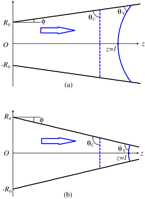
As the first example of an axially symmetric tube, we consider a conical tube (Fig. 1) whose radius changes according to
| (36) |
where corresponds to a converging and to a diverging tube.
This simple conical tube acts as a liquid diode, namely, the converging direction acts as the forward and the diverging direction acts as the reverse direction of the electronic diode device Comanns et al. (2015); Singh, Kumar, and Khan (2020); Panter, Gizaw, and Kusumaatmaja (2020); Iwamatsu (2022); Xu et al. (2023); Iwamatsu (2023). Because spontaneous imbibition is possible only when the contact angle satisfies , where is a critical angle shown in Fig. 1, the spontaneous one-way transport toward the converging direction occurs when the contact angle satisfies since in a converging [Fig. 1(a)] and in a diverging [Fig. 1(b)] tube with being the tilt angle of the wall (). Therefore, a large tilt angle and, therefore, a non-slowly-varying conical tube is more advantageous to realize a liquid diode Iwamatsu (2022, 2023).
Here, we consider the transport to both directions so that we consider a wetting liquid with
| (37) |
with so that the spontaneous imbibition occurs by the action of capillary pressure in Eq. (31). Since , Eqs. (34) and (35) become
| (38) |
and Eq. (32) is written as
| (39) |
where
| (40) | |||||
Therefore, the non-slowly-varying perturbation parameter is and is absorbed into the denominator of Eq. (39), which is written as
| (41) |
By introducing non-dimensional variables and instead of and defined by
| (42) |
Equation (41) is transformed into
| (43) |
where the sign denotes the sign of . Equation (43) has been derived from Eq. (1) and used to derive various scaling laws of imbibition Reyssat et al. (2008); Urteaga et al. (2013); Iwamatsu (2022). Therefore, the perturbation of a non-slowly-varying radius is included only in the scaling for in Eq. (42) by the term proportional to in the denominator.
Equation (43) can be integrated and we have
| (44) |
which gives the time necessary to reach the position of a diverging tube with an inlet radius and to reach of a converging tube with an inlet radius
| (45) | |||||
| (46) |
They were originally obtained by Urteaga et al. Urteaga et al. (2013) [Eqs. (3) and (4)]. Note that since for a converging tube.
To compare the performance of a diverging and a converging conical tube of the same shape with the inlet radius and the outlet radius (), we note
| (47) |
where is the asymmetry of the conical tube. Then, the performance of the diverging conical tube in Eq. (45) should be compared not with the performance of the converging tube in Eq. (46) but with
| (48) |
derived from Eq. (46) by the transformation in Eq. (47). Since , for a converging tube..
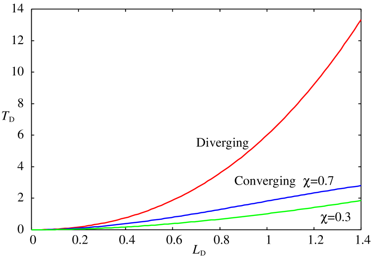
In Fig. 2, we compare the time that is necessary to reach the position of a diverging conical tube and that of a converging tube, where we use the scaling in Eq. (42) with the inlet radius of a diverging cone for both directions. Apparently, the flow in a converging tube is faster than that in a diverging tube, which was already pointed out Urteaga et al. (2013); Iwamatsu (2022). Here, we show that this conclusion is generic and does not depend on whether the radius of the tube is slowly-varying or not.
III.2 Capillary imbibition in a diverging power-law-shaped tube
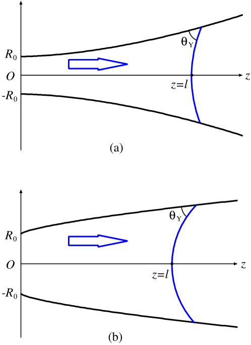
Next, we consider the general case of power-law-shaped diverging tubes shown in Fig. 3, whose radius changes according to
| (49) |
where the dimension of depends on the exponent . Reyssat et al. Reyssat et al. (2008) considered this problem and derived classical diffusive scaling law at an early stage and at a late stage. Apparently, the slowly-varying condition in Eq. (1) will be violated as at a late stage when [Fig. 3(a)]. Therefore, it is interesting to see if the effect of non-slowly-varying radius affects these scaling rules.
By introducing non-dimensional variables similar to those in Eq. (42) defined by
| (50) |
Equations. (33) to (35) will be written as
| (51) | |||||
| (52) | |||||
| (53) |
where
| (54) | |||||
| (55) | |||||
| (56) |
and the non-dimensional perturbation parameter for the diverging tube is given by
| (57) |
Therefore, the non-slowly-varying effect is determined from how rapidly the radius changes near the inlet. Then, Eq. (32) becomes
| (58) |
which determines the dynamics of the capillary flow in a diverging power-law-shaped tube when its radius is not necessarily slowly-varying.
It is straightforward to consider the asymptotic limit Reyssat et al. (2008) of Eq. (58). In an early stage , we have
| (59) | |||||
| (60) | |||||
| (61) |
Therefore, Eq. (58) becomes
| (62) |
in an early stage.
If the non-slip boundary condition is applicable (), the last term of the left-hand side of Eq. (62) disappears. When , the first term Eq. (62) is dominant and we recover the classical diffusive law
| (63) |
derived by Reyssat et al. Reyssat et al. (2008) When , no matter how small the perturbation parameter is, the second term of the left-hand side of Eq. (62) becomes dominant in an early stage and we have a new scaling rule
| (64) |
from the non-slowly-varying radius .
If the slip length cannot be negligible () and , no matter how large the perturbation parameter is, we can neglect the last two terms of the left-hand side of Eq. (62) and we find a classical diffusion law again:
| (65) |
When , on the other hand, the dominant term becomes the last term in Eq. (62) and we have a new scaling rule:
| (66) |
Therefore, a non-slowly-varying radius affects an early-stage scaling rule when and , and when and , and the scaling rules are given by Eqs. (64) and (66), respectively. They are different from the classical diffusive law in Eqs. (63) and (65) derived by Reyssat et al. Reyssat et al. (2008)
Similarly, at a late stage , Eq. (58) can be approximately written as
| (67) |
because , , and are all finite. Therefore, at a late stage
| (68) |
which has been found previously by Reyssat et al. Reyssat et al. (2008) using the slowly-varying approximation in Eq. (1). As far as the asymptotic limit at a late stage is concerned, the effect of perturbation does not affect the scaling rule in Eq. (68). Therefore, even if the radius is not necessarily slowly varying, the power-law-shaped tube shows the same scaling rule at a late stage.
III.3 Capillary imbibition in a converging power-law-shaped tube
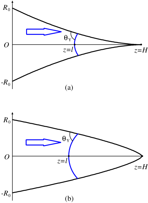
Gorce et al. Gorce, Hewitt, and Vella (2016) have studied converging power-law-shaped tubes whose radius changes as
| (69) |
where is the length of the converging tube. Typical shapes are shown in Fig. 4 where we show the tube shape for and . It is assumed that there is a small hole at the outlet at so that the fluid can flow out from the tube and any divergence associated with as is neglected. They Gorce, Hewitt, and Vella (2016) showed that the flow rate can be faster than that in a straight cylindrical tube beating classical Washburn’s law Washburn (1921). Furthermore, there exists the optimal index for which the imbibition time is shortest. We will see how their results Gorce, Hewitt, and Vella (2016) will be modified by the non-slowly-varying effect.
By introducing the non-dimensional variables
| (70) |
Equation (33) becomes
| (71) | |||||
Similarly, Eqs. (34) and (35) become
| (72) | |||||
| (73) |
where the perturbation parameter for the converging tube is defined by
| (74) |
whose meaning is apparent.
Using these non-dimensional variables in Eq. (70), Eq. (32) is written as
| (75) |
which can be integrated and the time necessary to reach is given by
| (76) | |||||
with
| (77) |
is a new perturbation parameter, and
| (78) |
is the time necessary to reach the outlet at . We can recover the result of Gorce et al. Gorce, Hewitt, and Vella (2016) when in Eq. (78) ]The scaling used by them Gorce, Hewitt, and Vella (2016) is slightly different from Eq. (70)].
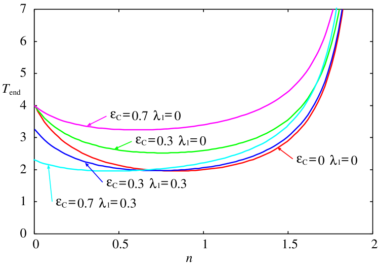
Figure 5 shows the time as a function of the exponent . It has a limiting value
| (79) |
and shows a minimum, which occurs at
| (80) |
obtained by minimizing Eq. (78). In the slowly-varying limit
| (81) |
which was derived Gorce, Hewitt, and Vella (2016) using the slowly-varying approximation in Eq. (1).
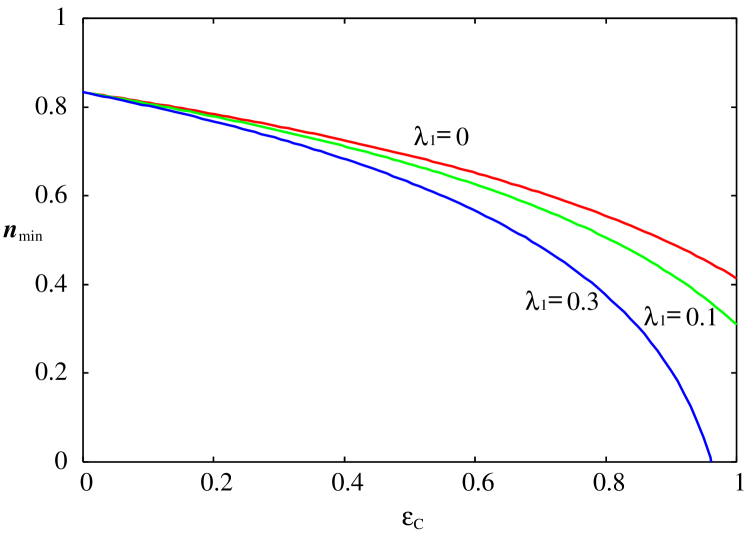
In Fig. 6, we show as a function of the perturbation parameter . As the non-slowly-varying perturbation is larger, the optimal exponent becomes smaller so that the optimal shape of the tube is fatter [Fig. 4(b). Of course, the practical problem of fabrication and fine tuning of the exponent may not be easy.
IV Conclusion
In this study, we considered the capillary flow in an axially symmetric tube of a non-slowly-varying radius. We also considered the Navier’s boundary slip and used the hydrodynamic model Duarte, Strier, and Zanette (1996); Digilov (2008); Liou, Peng, and Parker (2009); Wang, Graber, and Wallach (2013); Nissan, Wang, and Wallach (2016) to derived macroscopic equation for the capillary flow from the Stokes equation. The new formula derived is a direct extension of the popular Hagen-Poiseulle law for the capillary flow in a tube of a slowly-varying radius G. K. Batchelor (1967) which has been widely used Sharma and Ross (1991); Staples and Shaffe (2002); Young (2004); Reyssat et al. (2008); Urteaga et al. (2013); Berli and Urteaga (2014); Elizalde et al. (2014); Gorce, Hewitt, and Vella (2016).
Using this newly derived formula, we reconsidered the dynamics of meniscus by the capillary imbibition and the extension of the classical Lucas-Washburn scaling law Lucas (1918); Washburn (1921) in several typical geometries. We found that the capillary imbibition in a converging and a diverging conical tube is not affected by the non-slowly-varying effect, so that the conical tube shows a diode-like asymmetric transport Urteaga et al. (2013); Berli and Urteaga (2014); Singh, Kumar, and Khan (2020); Iwamatsu (2022) even if its radius varies not slowly. We also considered the capillary imbibition in a diverging Reyssat et al. (2008) and a converging Gorce, Hewitt, and Vella (2016) power-law-shaped tube and identified the perturbation parameter which characterizes the non-slowly-varying radius. In those cases, the imbibition is affected by a non-slowly-varying radius so that their scaling laws and optimal shapes could be modified if the non-slowly-varying effect is important. Our results will supplement the popular formula G. K. Batchelor (1967) widely used and will be useful to assess the fluid transport ability of axially symmetric tubes with non-slowly-varying cross sections.
Author Declaration
Conflict of interest
The author declares no conflict of interest.
Data Availability Statement
The data that support the findings of this study are available from the author upon reasonable request.
References
- G. K. Batchelor (1967) F. G. K. Batchelor, An Introduction to Fluid Dynamics (Cambridge UP, Cambridge, 1967).
- Cai et al. (2022) J. Cai, Y. Chen, Y. Liu, S. Li, and C. Sun, “Capillary imbibition and flow of wetting liquid in irregular capillaries: A 100-year review,” Adv. Colloid Interface Sci. 304, 102654 (2022).
- Prakash, Quéré, and Bush (2008) M. Prakash, D. Quéré, and J. W. M. Bush, “Surface tension transport of prey by feeding shorebirds: The capillary ratchet,” Science 320, 931 (2008).
- Kim and Bush (2012) W. Kim and J. W. M. Bush, “Natural drinking strategies,” J. Fluid. Mech. 705, 7 (2012).
- Squires and Quake (2005) T. M. Squires and S. R. Quake, “Microfluidics: Fluid physics at the nanoliter scale,” Rev. Mod. Phys. 77, 977 (2005).
- Bocquet and Charlaix (2010) L. Bocquet and E. Charlaix, “Nanofluids, from bulk to interfaces,” Chem. Soc. Rev. 39, 1073 (2010).
- Kavokine, Netz, and Bocquet (2021) N. Kavokine, R. R. Netz, and L. Bocquet, “Fluids at the nanoscale: from continuum to subcontinuum transport,” Annu. Rev. Fluid Mech. 53, 377 (2021).
- Comanns et al. (2015) P. Comanns, G. Buchberger, A. Buchsbaum, R. Baumgartner, A. Kogler, S. Bauer, and W. Baumgartner, “Directional, passive liquid transport: the texas horned lizard as a model for a biomimetic ’liquid diode’,” J. Roy. Soc. Interface 12, 20150415 (2015).
- Bell and Cameron (1906) J. M. Bell and F. K. Cameron, “The flow of liquid through capillary spaces,” J. Phys. Chem. 10, 658 (1906).
- Lucas (1918) R. Lucas, “Ueber das zeitgesetz des kapillaren aufstiegs von flüssigkeiten,” Kolloid Z. 23, 15 (1918).
- Washburn (1921) E. W. Washburn, “The dynamics of capillary flow,” Phys. Rev. 17, 273 (1921).
- Rideal (1922) E. K. Rideal, “On the flow of liquids under capillary pressure,” Phil. Mag. 44, 1152 (1922).
- Bosanquet (1923) C. H. Bosanquet, “On the flow of liquids into capillary tubes,” Phil. Mag. 45, 525 (1923).
- Landau and Lifshitz (1987) L. D. Landau and E. M. Lifshitz, Fluid Mechanics, 2nd ed. (Elsevier, Amsterdam, 1987).
- de Gennes, Brochard-Wyart, and Quéré (2004) P.-G. de Gennes, F. Brochard-Wyart, and D. Quéré, Capillarity and Wetting Phenomena Drops, Bubbles, Pearls, Waves (Springer, New York, 2004).
- Sharma and Ross (1991) R. Sharma and D. S. Ross, “Kinetics of liquid penetration into periodically constrained capillaries,” J. Chem. Soc. Faraday Trans. 87, 619 (1991).
- Staples and Shaffe (2002) T. L. Staples and D. G. Shaffe, “Wicking flow in irregular capillaries,” Colloid Surf A 204, 239 (2002).
- Young (2004) W.-B. Young, “Analysis of capillary flow in non-uniform cross-sectional capillaries,” Colloid Surf A 234, 123 (2004).
- Reyssat et al. (2008) M. Reyssat, L. Courbin, E. Reyssat, and H. A. Stone, “Imbibition in geometries with axial variation,” J. Fluid Mech. 615, 335 (2008).
- Urteaga et al. (2013) R. Urteaga, L. N. Acquaroli, R. R. Koropecki, A. Santos, M. Alba, J. Pallarès, L. F. Marsal, and C. L. A. Berli, “Optofluidic characterization of nanoporous membranes,” Langmuir 29, 2784 (2013).
- Berli and Urteaga (2014) C. L. A. Berli and R. Urteaga, “Asymmetric capillary filling of non-newtonian power law fluids,” Microfluid Nanofluid 17, 1079 (2014).
- Elizalde et al. (2014) E. Elizalde, R. Urteaga, R. R. Koropecki, and C. L. A. Berli, “Inverse problem of capillary filling,” Phys. Rev. Lett. 112, 134502 (2014).
- Gorce, Hewitt, and Vella (2016) J.-B. Gorce, I. J. Hewitt, and D. Vella, “Capillary imbibition into converging tubes: Beating washburn’s law and the optimal imbibition of liquids,” Langmuir 32, 1560 (2016).
- Khatoon, Phirani, and Bahga (2020) S. Khatoon, J. Phirani, and S. S. Bahga, “An analytical solution of the inverse problem of capillary imbibition,” Phys Fluids 32, 041704 (2020).
- Tran-Duc, Phan-Thien, and Thamwattana (2020) T. Tran-Duc, N. Phan-Thien, and N. Thamwattana, “On permeability of corrugated pore membranes,” AIP Adv. 10, 045317 (2020).
- Iwamatsu (2022) M. Iwamatsu, “Thermodynamics and hydrodynamics of spontaneous and forced imbibition in conical capillaries: A theoretical study of conical liquid diode,” Phys. Fluids 34, 047119 (2022).
- Tran-Duc, Phan-Thien, and Wang (2019) T. Tran-Duc, N. Phan-Thien, and J. Wang, “A theoretical study of permeability enhancement for ultrafiltration ceramic membranes with conical pores and slippag,” Phys. Fluids 31, 022003 (2019).
- Mondal et al. (2021) N. Mondal, A. Chaudhuri, C. Bakli, and S. Chakraborty, “Upstream events dictate interfacial slip in geometrically converging nanopores,” J. Chem. Phys. 154, 164709 (2021).
- Duarte, Strier, and Zanette (1996) A. A. Duarte, D. E. Strier, and D. H. Zanette, “The rise of a liquid in a capillary tube revisited: A hydrodynamical approach,” Am. J. Phys. 64, 413 (1996).
- Digilov (2008) R. M. Digilov, “Capillary rise of a non-newtonian power law liquid: Impact of the fluid rheology and dynamic contact angle,” Langmuir 24, 13663 (2008).
- Liou, Peng, and Parker (2009) W. W. Liou, Y. Peng, and P. E. Parker, “Analytical modeling of capillary flow in tubes of nonuniform cross section,” J. Colloid Interface Sci. 333, 389 (2009).
- Wang, Graber, and Wallach (2013) Q. Wang, E. R. Graber, and R. Wallach, “Synergistic effects of geometry, inertia, and dynamic contact angle on wetting and dewetting of capillaries of varying cross sections,” J. Colloid Interface Sci. 396, 270 (2013).
- Nissan, Wang, and Wallach (2016) A. Nissan, Q. Wang, and R. Wallach, “Kinetics of gravity-driven slug flow in partially wettable capillaries of varying cross section,” Water Resour. Res. 52, 8472 (2016).
- Menon and Agrawal (1987) V. J. Menon and D. C. Agrawal, “Newton’s law of motion for variable mass systems applied to capillarity,” Am. J. Phys. 55, 63 (1987).
- Zhmud, Tiberg, and Hallstensson (2000) B. V. Zhmud, F. Tiberg, and K. Hallstensson, “Dynamics of capillary rise,” J. Colloid Interface Sci. 228, 263 (2000).
- Masoodi, Languri, and Ostadhossein (2013) R. Masoodi, E. Languri, and A. Ostadhossein, “Dynamics of liquid rise in a vertical capillary tube,” J. Colloid Interface Sci. 389, 268 (2013).
- Majumder et al. (2005) M. Majumder, N. Chopra, R. Andrews, and B. J. Hinds, “Enhanced flow in carbon nanotubes,” Nature 438, 44 (2005).
- Neto et al. (2005) C. Neto, D. R. Evans, E. Bonaccurso, H.-J. Butt, and V. S. J. Craig, “Boundary slip in newtonian liquids: a review of experimental studies,” Rep. Prog. Phys. 68, 2859 (2005).
- Suk and Aluru (2017) M. E. Suk and N. R. Aluru, “Modeling water flow through carbon nanotube membranes with entrance/exit effects,” Nanoscale Microscale Thermophys. Eng. 21, 247 (2017).
- Wu et al. (2017) K. Wu, Z. Chena, J. Lib, X. Lib, J. Xua, and X. Dong, “Intrusion and extrusion of water in hydrophobic nanopores,” Proc. Natl. Acad. Sci. USA 114, 3358 (2017).
- Wu, Nikolov, and Wasan (017a) P. Wu, A. Nikolov, and D. Wasan, “Capillary dynamics driven by molecular self-layering,” Adv. Colloid Interface Sci. 243, 114 (2017a).
- Popescu, Ralston, and Sedev (2008) M. N. Popescu, J. Ralston, and R. Sedev, “Capillary rise with velocity-dependent dynamic contact angle,” Langmuir 24, 12710 (2008).
- Wu, Nikolov, and Wasan (017b) P. Wu, A. D. Nikolov, and D. T. Wasan, “Capillary rise: Validity of the dynamic contact angle models,” Langmuir 33, 7862 (2017b).
- Sampson (1891) R. A. Sampson, “On stokes’s current function,” Phil. Trans. Roy. Soc. London A 182, 449 (1891).
- Weissberg (1962) H. L. Weissberg, “End correction for slow viscous flow through long tubes,” Phys. Fluids 5, 1033 (1962).
- Kornev and Neimark (2000) K. G. Kornev and A. V. Neimark, “Spontaneous penetration of liquids into capillaries and porous membranes revisited,” J. Colloid Interface Sci. 235, 101 (2000).
- Stange, Dreyer, and Rath (2003) M. Stange, M. E. Dreyer, and H. J. Rath, “Capillary driven flow in circular cylindrical tubes,” Phys. Fluids 15, 2587 (2003).
- Willmott, Neto, and Hendy (2011) G. R. Willmott, C. Neto, and S. C. Hendy, “Uptake of water droplets by nonwetting capillaries,” Soft Matters 7, 2357 (2011).
- Scholle, Wierschem, and Aksel (2004) M. Scholle, A. Wierschem, and N. Aksel, “Creeping films with vortices over strongly undulated bottoms,” Acta Mech. 168, 167 (2004).
- Marner, Gaskell, and Scholle (2017) F. Marner, P. H. Gaskell, and M. Scholle, “A complex-valued first integral of navier-stokes equations: Unsteady couette flow in a corrugated channel system,” J. Math. Phys. 58, 043102 (2017).
- Goli, Saha, and Agrawal (2022) S. Goli, S. K. Saha, and A. Agrawal, “Physics of fluid flow in an hourglass (converging-diverging) microchannel,” Phys. Fluids 34, 052006 (2022).
- Singh, Kumar, and Khan (2020) M. Singh, A. Kumar, and A. R. Khan, “Capillary as a liquid diode,” Phys. Rev. Fluids 5, 102101(R) (2020).
- Panter, Gizaw, and Kusumaatmaja (2020) J. R. Panter, Y. Gizaw, and H. Kusumaatmaja, “Critical pressure asymmetry in the enclosed fluid diode,” Langmuir 36, 7463 (2020).
- Xu et al. (2023) B. Xu, S. Min, Y. Ding, H. Chen, and Q. Zhu, “Multi-pores janus paper with unidirectional liquid transport property toward information encryption/decryption,” Colloid Surf. A 664, 131133 (2023).
- Iwamatsu (2023) M. Iwamatsu, “Thermodynamics of imbibition in capillaries of double conical structures-hourglass, diamond, and sawtooth shaped capillaries,” Phys. Fluids 35, 092009 (2023).