Estimating Complier Average Causal Effects with Mixtures of Experts

Abstract

Understanding the causal impact of medical interventions is essential in healthcare research, especially through randomized controlled trials (RCTs). Despite their prominence, challenges arise due to discrepancies between treatment allocation and actual intake, influenced by various factors like patient non-adherence or procedural errors. This paper focuses on the Complier Average Causal Effect (CACE), crucial for evaluating treatment efficacy among compliant patients. Existing methodologies often rely on assumptions such as exclusion restriction and monotonicity, which can be problematic in practice. We propose a novel approach, leveraging supervised learning architectures, to estimate CACE without depending on these assumptions. Our method involves a two-step process: first estimating compliance probabilities for patients, then using these probabilities to estimate two nuisance components relevant to CACE calculation. Building upon the principal ignorability assumption, we introduce four $\sqrt{n}-$consistent, asymptotically normal, CACE estimators, and prove that the underlying mixtures of experts’ nuisance components are identifiable. Our causal framework allows our estimation procedures to enjoy reduced mean squared errors when exclusion restriction or monotonicity assumptions hold. Through simulations and application to a breastfeeding promotion RCT, we demonstrate the method’s performance and applicability.

1 Introduction

In healthcare, it is increasingly important to understand the causal impact of medical interventions (Prosperi et al., 2020). At the heart of this investigation are randomized controlled trials, the cornerstone of clinical research, characterized by a predetermined allocation probability for treatment assignment. With this in mind, recent guidelines, such as the international ICH E9 guidelines, have highlighted the need for meticulous definition and clarification of estimands in these trials (International Council For Harmonisation of Technical Requirements For Pharmaceuticals For Human Use (2019), ICH). In clinical trials, one major challenge is the frequent discrepancy between the treatment allocated to a patient and the treatment they effectively take. This gap is often attributed to a multitude of factors, including logistical errors by medical staff, patient-related factors such as non-adherence to treatment due to adverse effects, the complexity of existing drug regimens or personal beliefs. To address this issue, this paper focuses on a key estimand known as the Complier Average Causal Effect (CACE) (Frangakis and Rubin, 1999; Little and Rubin, 2000) also termed Local Average Treatment Effect in econometrics (Imbens and Angrist, 1994; Angrist et al., 2000; Heckman and Vytlacil, 2001).

The CACE is a crucial tool to evaluate the effect of an experimental treatment versus control, only among patients who will follow the treatment as allocated. Following the principal stratification approach of Frangakis and Rubin (2002), four distinct strata of compliance are defined: (i) compliers who adhere to the assigned treatment; (ii) never-takers who always follow the control treatment regardless of assignment; (iii) always-takers who always follow the experimental treatment regardless of assignment; (iv) defiers who do the opposite of their assignment. The challenge is that identifying the stratum of a patient requires knowledge of the treatment they would take in both experimental and control arms. However, only the treatment received in the assigned arm is observed and therefore, the stratum of a patient can be viewed as a latent variable.

The use of instrumental variables is a popular method to address this challenge (Angrist et al., 1996; Imbens, 2014). Typically, these methodologies for CACE estimation rely on two main assumptions: exclusion restriction, which assumes that the act of allocation itself has no direct effect on the outcome beyond the administered treatment, and monotonicity, often encapsulated in the ‘no defiers’ assumption, which posits that no patients systematically opt for the opposite treatment to the one they are allocated to (Stuart and Jo, 2015). The validity of the monotonicity assumption can be challenging to ascertain with empirical data, while the exclusion restriction premise is particularly susceptible to violations in open-label trials, as evidenced by the phenomenon of performance bias (Mansournia et al., 2017). To our knowledge, no general causal model has been proposed to estimate CACE without assumptions of exclusion restriction or monotonicity in a frequentist inference framework. Imbens and Rubin (1997) have made significant contributions by developing a general causal model suitable for CACE estimation. However, the identifiability of their model has not been studied, and the proposed parametric Bayesian CACE estimation procedure remains rarely used in practice.

In this paper, we revisit Imbens and Rubin (1997) work so that we can leverage architectures from the field of (frequentist) supervised learning. Toward that end, we present a comprehensive causal model designed to estimate the CACE without depending on traditional assumptions such as exclusion restriction or monotonicity. Then, we propose methods for estimating the CACE via mixture of experts models, whose (possibly infinite-dimensional) parameters are obtained using expectation-maximization (EM) algorithms (Jordan and Jacobs, 1994). Our appproach consists of two distinct steps. First, we focus on estimating the probabilities of each patient being in the four distinct strata of compliance. Then, in a second step, we leverage this conditional probability distribution to successively estimate two nuisance components (called the conditional elementary potential outcome functions) that are relevant to CACE calculation. Our approach is based on the principal ignorability assumption (Jo and Stuart, 2009), which postulates that the key information defining compliance is encapsulated in patients’ baseline covariates. This two-step approach is designed to produce consistent, robust and more accurate estimates of CACEs.

This article is organized as follows: Section 2 introduces a causal model and the underlying assumptions necessary for CACE estimation. In section 3, we describe and justify our two-step estimation procedure. In section 4, we discuss the possible incorporation of the exclusion restriction and monotonicity assumptions to reduce mean squared errors. In section 5, we conduct simulations to study the properties of four different estimation procedures under possible violations of the underlying assumptions. In section 6, we apply our methods to a simulated randomized controlled trial that evaluated the promotion of breastfeeding to maximize infants’ health (Goetghebeur et al., 2020). Section 7 concludes with some discussion of extensions. In the Appendix, we provide key identifiability results for the models underlying our estimation procedures. The computer code reproducing the experiments shown in this paper is available at https://github.com/fcgrolleau/CACEmix.

2 Setup

2.1 A probability model for the data generating mechanism

We denote by $X$ the patients’ baseline (i.e., pre-randomization) covariates, and by $Z$ their allocated binary treatment. We formalize the concept of a randomized controlled trial via the following assumption.

Assumption 1 (Random allocation)

For any realized value of covariates, individuals could be allocated to either treatment option. That is, the allocated treatment is generated as

$$Z|X\sim\textit{Bernoulli}(p=\eta(X))$$

where $\eta(\cdot)$, the allocation ratio function of the randomized controlled trial , is such that the following holds:

$$\exists\epsilon_{\eta}\in\mathbb{R},\quad\forall x\in\mathcal{X},\quad 0<\epsilon_{\eta}<\eta(x)<1-\epsilon_{\eta}<1.$$

To characterize the notions of complier, always taker, never taker, and defier patients we introduce the following potential treatments:

$$T^{s=c}\operatorname*{\stackrel{{\scriptstyle\text{def}}}{{=}}}Z,\quad T^{s=a}\operatorname*{\stackrel{{\scriptstyle\text{def}}}{{=}}}1,\quad T^{s=n}\operatorname*{\stackrel{{\scriptstyle\text{def}}}{{=}}}0,\quad\text{and}\quad T^{s=d}\operatorname*{\stackrel{{\scriptstyle\text{def}}}{{=}}}1-Z.$$

These potential treatments correspond to the treatment that a complier, an always taker, a never taker, and a defier would take respectively. In the notation above, the s superscript indicates the “stratum” of a patient i.e., complier, always taker, never taker, or defier. Since the strata are not observed in practice, throughout this paper, we consider it a latent variable. For later convenience, we introduce the latent stratum of a patient as the one-hot-encoded random vector $\boldsymbol{S}=(S_{c},S_{a},S_{n},S_{d})^{T},$ where the vectors $(1,0,0,0)^{T}$, $(0,1,0,0)^{T}$, $(0,0,1,0)^{T}$, $(0,0,0,1)^{T}$ indicate that a patient is a complier, an always taker, a never taker, and a defier respectively. We further define the conditional probabilities that a patient is a complier, an always taker, a never taker, and a defier as $\rho_{c}(X)\operatorname*{\stackrel{{\scriptstyle\text{def}}}{{=}}}\operatorname{\mathbb{E}}(S_{c}|X)$, $\rho_{a}(X)\operatorname*{\stackrel{{\scriptstyle\text{def}}}{{=}}}\operatorname{\mathbb{E}}(S_{a}|X)$, $\rho_{n}(X)\operatorname*{\stackrel{{\scriptstyle\text{def}}}{{=}}}\operatorname{\mathbb{E}}(S_{n}|X)$, and $\rho_{d}(X)\operatorname*{\stackrel{{\scriptstyle\text{def}}}{{=}}}\operatorname{\mathbb{E}}(S_{d}|X)$ respectively. We note that if a patient’s stratum and their allocated treatment were known, then the treatment they effectively took would be entirely characterized. To account for this fact, we define the treatment effectively taken $T$ as follows.

Definition 1 (Treatment effectively taken)

The treatment effectively taken $T$ is consistent with potential treatments in the sense that

$$T \operatorname*{\stackrel{{\scriptstyle\text{def}}}{{=}}}S_{c}T^{s=c}+S_{a}T^{s=a}+S_{n}T^{s=n}+S_{d}T^{s=d}$$

$$=S_{c}Z+S_{a}+S_{d}(1-Z).$$ (1)

We suppose the existence of elementary potential outcomes of the form $Y^{s=k,z=l,t=m}$ corresponding to the outcome that would be observed if a patient stratum had been $k,$ their allocated treatment $l,$ and their treatment effectively taken $m.$ Although this may appear complex, these elementary potential outcomes serve the purpose of characterizing the standard potential outcomes while relaxing usual assumptions of exclusion restriction and monotonicity. The standard potential outcomes $Y^{t=1}$ and $Y^{t=0},$ represent the outcome a patient would achieve if they had taken treatment option $T=0$ or $T=1$ respectively. In this paper, we define the potential outcomes as follows.

Definition 2 (Potential outcomes)

The potential outcomes $Y^{t=1}$ and $Y^{t=0}$ are consistent with elementary potential outcomes in the sense that

$$Y^{t=1}\operatorname*{\stackrel{{\scriptstyle\text{def}}}{{=}}}S_{c}Y^{s=c,z=1,t=1}+S_{a}ZY^{s=a,z=1,t=1}+S_{a}(1-Z)Y^{s=a,z=0,t=1}+S_{d}Y^{s=d,z=0,t=1},$$

$$Y^{t=0}\operatorname*{\stackrel{{\scriptstyle\text{def}}}{{=}}}S_{c}Y^{s=c,z=0,t=0}+S_{n}ZY^{s=n,z=1,t=0}+S_{n}(1-Z)Y^{s=n,z=0,t=0}+S_{d}Y^{s=d,z=1,t=0}.$$

Note that this definition for $Y^{t=1}$ and $Y^{t=0}$ should not be viewed as a causal assumption as it does not impose any conceptual constraint. In fact, with this definition the potential outcome $Y^{t=1}$ of an alway-taker could be different depending on whether their allocated treatment was $Z=0$ or $Z=1$; that is, we do not impose $Y^{s=a,z=0,t=1}$ and $Y^{s=a,z=1,t=1}$ to be equal. Likewise, the potential outcome $Y^{t=0}$ of a never-taker could be different depending on whether their allocated treatment was $Z=0$ or $Z=1$. In other words, our model does not make an exclusion restriction assumption. Moreover, in Definition 2 the defiers’ potential outcomes are explicitly taken into account and hence, our model does not make a monotonicity assumption. In section 4, we will consider the particular situations where the exclusion restriction and/or monotonicity assumptions hold. We introduce the observed outcomes $Y$ by appealing to the standard consistency assumption.

Assumption 2 (Consistency)

The observed outcomes are consistent with potential outcomes, in the sense that

$$Y=TY^{t=1}+(1-T)Y^{t=0}.$$

To identify complier average causal effects, we also rely on the principal ignorablity and positivity of compliers assumptions.

Assumption 3 (Principal ignorablity)

The following two conditional independance statements hold.

• All variables causing the stratum $\boldsymbol{S}$ and the allocated treatment $Z$ are measured, i.e.,

  $$Z\perp\!\!\!\perp\boldsymbol{S}|X.$$

• All variables causing the stratum $\boldsymbol{S}$ and the elementary potential outcomes are measured, i.e., $\forall(k,l,m)\in\{c,a,n,d\}\times\{0,1\}\times\{0,1\}$

  $$Y^{s=k,z=l,t=m}\perp\!\!\!\perp\boldsymbol{S}|X.$$

In a randomized controlled trial, the first conditional independance statement is a weak assumption that often holds by design. The second statement of principal ignorablity may be viewed as an adaptation of the usual no unmeasured confounders assumption (Rubin, 1978) to the context of imperfect compliance.

Assumption 4 (Positivity of compliers)

There exists a constant $\epsilon_{\rho}>0$ such that the following holds:

$$\forall x\in\mathcal{X},\quad\rho_{c}(x)>\epsilon_{\rho}.$$

The positivity of compliers assumption may be viewed as an adaptation of the usual positivity assumption (Rosenbaum and Rubin, 1983) to the context of imperfect compliance. In practice, assuming that assumptions 1, 3, and 4 hold guarantees that all conditional expectations introduced in the next subsection are well-defined.

2.2 Notations

For $k\in\{c,a,n,d\}$, $l\in\{0,1\}$ and $m\in\{0,1\},$ we define the conditional probability functions

$$P_{klm}(x) \operatorname*{\stackrel{{\scriptstyle\text{def}}}{{=}}}\operatorname{\mathbb{E}}(S_{k}|Z=l,T=m,X=x),$$

the conditional observed outcome functions

$$q_{lm}(x) \operatorname*{\stackrel{{\scriptstyle\text{def}}}{{=}}}\operatorname{\mathbb{E}}(Y|Z=l,T=m,X=x),$$

and the conditional elementary potential outcome functions

$$Q_{klm}(x) \operatorname*{\stackrel{{\scriptstyle\text{def}}}{{=}}}\operatorname{\mathbb{E}}(Y^{s=k,z=l,t=m}|X=x).$$

For clarity, we denote the standard propensity score by $e(X)\operatorname*{\stackrel{{\scriptstyle\text{def}}}{{=}}}\operatorname{\mathbb{E}}[T|X]$ and its relevant adaptation in the context of imperfect compliance is denoted by $\pi(X,Z)\operatorname*{\stackrel{{\scriptstyle\text{def}}}{{=}}}\operatorname{\mathbb{E}}(T|X,Z).$ A summary of the notations used in this paper is provided in Appendix A.

2.3 The CACE estimand

Our target estimand, the CACE, is defined as $\Delta\operatorname*{\stackrel{{\scriptstyle\text{def}}}{{=}}}\operatorname{\mathbb{E}}(Y^{t=1}-Y^{t=0}|S_{c}=1).$ In this paper, we make use of the following rearrangement.

Lemma 1

Under assumptions 3 and 4, the CACE estimand can be represented as

$$\Delta=\operatorname{\mathbb{E}}\Big{[}\big{\{}Q_{c11}(X)-Q_{c00}(X)\big{\}}\rho_{c}(X)\Big{]}/\operatorname{\mathbb{E}}[\rho_{c}(X)].$$

A proof of this lemma is included in Appendix B. The goal of the inference procedure described in the next section is to estimate the functions $Q_{c11}$, $Q_{c00}$, and $\rho_{c}$ in order to derive a plug-in estimator for $\Delta$.

3 Inference

We consider the experiment $(X_{i},\boldsymbol{S_{i}},Z_{i},T_{i},Y_{i})\stackrel{{\scriptstyle\text{iid}}}{{\sim}}\mathcal{P}$ where we only observe $(X_{i},Z_{i},T_{i},Y_{i})_{1\leq i\leq n}$ as $\boldsymbol{S_{i}}$, the stratum of a patient, is considered a latent variable. An overview of our estimation procedure can be found in Algorithm 3.1. Below, we explain the main steps involved.

3.1 Step 1: joint estimation of the functions $\rho_{k}(\cdot)_{k\in\{c,a,n,d\}}$

First, we will estimate the function $\rho_{c}$ by making use of the following expression for the propensity score $\pi$.

Lemma 2

Under assumptions 1 and 3, the mechanism generating the treatment effectively taken is given by

$$\pi(X,Z)=\sum_{k\in\{c,a,n,d\}}\rho_{k}(X)\mu_{k}(Z)$$

where $\mu_{k}(Z)\operatorname*{\stackrel{{\scriptstyle\text{def}}}{{=}}}\operatorname{\mathbb{E}}(T^{s=k}|Z).$

A proof of this lemma is included in Appendix B. Lemma 2 suggests that the propensity score $\pi(\cdot)$ can be viewed as mixture of the known experts $\mu_{c}(z)=z$, $\mu_{a}(z)=1$, $\mu_{n}(z)=0$, $\mu_{d}(z)=1-z$, while the proportions of the mixture are given by the unknown gating network $\rho_{k}(\cdot)_{k\in\{c,a,n,d\}}$. In Theorem D.19 (Appendix D), we show that, under parametric assumptions, the mixture of expert model for $\pi(x,z)$ in Lemma 2 is identifiable. Jordan and Jacobs (1994) described procedures to fit mixture of experts. For instance, if the functions $\rho_{k}(\cdot)_{k\in\{c,a,n,d\}}$ are assumed to be differentiable with respect to some parameters then, fitting can be achieved in the supervised learning paradigm by specifying the relevant (mixture) architecture and minimizing via gradient descent a binary cross-entropy loss function with targets $(A_{i})_{1\leq i\leq n}$. Alternatively, we propose to jointly estimate $\rho_{k}(\cdot)_{k\in\{c,a,n,d\}}$ via the procedure given in Algorithm C.1. This procedure details an EM algorithm, based on the description from Xu and Jordan (1993) for fitting a mixture of known experts. In Algorithm C.4, we provide an adaptation of this EM-procedure that allows to fit nonparametric and/or non-differentiable functions for $\rho_{k}(\cdot)_{k\in\{c,a,n,d\}}$.

3.2 Step 2: parallel estimation of the functions $\{Q_{c11},\,Q_{a11}\}$ and $\{Q_{c00},\,Q_{n00}\}$

Next, we make use of the following rearrangement of the conditional observed outcome functions $q_{11}$ and $q_{00}$ to estimate $Q_{c11}$, and $Q_{c00}$ separately.

Lemma 3

Suppose that assumptions 1, 2, 3 and 4 hold. Then,

$$(i)\quad q_{11}(X) =P_{c11}(X)Q_{c11}(X)+P_{a11}(X)Q_{a11}(X),$$

$$(ii)\quad q_{00}(X) =P_{c00}(X)Q_{c00}(X)+P_{n00}(X)Q_{n00}(X).$$

A proof of this lemma is included in Appendix B. Furthermore, we can use Bayes’ rule to verify the following lemma.

Lemma 4

Under assumptions 1, 3 and 4, the conditional probability functions $P_{c11}$, $P_{a11}$, $P_{c00}$, $P_{n00}$ can be represented as

$$(a)\quad P_{c11}(X) =\rho_{c}(X)/\{\rho_{c}(X)+\rho_{a}(X)\},$$

$$(b)\quad P_{a11}(X) =\rho_{a}(X)/\{\rho_{c}(X)+\rho_{a}(X)\},$$

$$(c)\quad P_{c00}(X) =\rho_{c}(X)/\{\rho_{c}(X)+\rho_{n}(X)\},$$

$$(d)\quad P_{n00}(X) =\rho_{n}(X)/\{\rho_{c}(X)+\rho_{n}(X)\}.$$

A proof of this lemma is included in Appendix B. Equation (i) in Lemma 3 suggests that the conditional expectation $q_{11}(\cdot)$ can be viewed as a mixture of the unknown (expert) functions $Q_{c11}(\cdot)$ and $Q_{a11}(\cdot)$. In addition, in Lemma 4, equations (a) and (b) suggest that the proportions for this mixture, i.e., the gating network $\{P_{c11}(\cdot),P_{a11}(\cdot)\}$, are known, if $\rho_{k}(\cdot)_{k\in\{c,a,n,d\}}$ are known. Since $\rho_{k}(\cdot)_{k\in\{c,a,n,d\}}$ are estimated by the end of Step 1, we propose to estimate this gating network via

$$\quad\hat{P}_{c11}(X_{i}) =\hat{\rho}_{c}(X_{i})/\{\hat{\rho}_{c}(X_{i})+\hat{\rho}_{a}(X_{i})\}, \quad\hat{P}_{a11}(X_{i}) =1-\hat{P}_{c11}(X_{i}).$$

In Theorem D.22 (Appendix D), we show that, assuming $Q_{kll}(\cdot)$ are linear parametric functions, the mixtures of the form shown in Lemma 3 are identifiable. In Theorem D.24 (Appendix D), we prove under regularity conditions that these mixtures are also identifiable, if we assume that $Q_{kll}(\cdot)$ are expit functions. Adapting the fitting algorithm of Xu and Jordan (1993), we propose to jointly estimate $Q_{c11}(\cdot)$ and $Q_{a11}(\cdot)$ via the EM-procedure given in Algorithm C.2, when the outcome $Y$ is binary. This algorithm takes $(X_{i},Y_{i},\hat{P}_{c11}(X_{i}))_{i:Z_{i}=1,T_{i}=1}$ as input and intuitively, it distinguishes between the compliers and the always takers within the subset $\{Z=1,T=1\}$. Likewise, considering equation (ii) from Lemma 3, we propose to jointly estimate $Q_{c00}(\cdot)$ and $Q_{n00}(\cdot)$ by providing $(X_{i},Y_{i},\hat{P}_{c00}(X_{i}))_{i:Z_{i}=0,T_{i}=0}$ as input to Algorithm C.2. Intuitively, Algorithm C.2 then attempts to distinguish between the compliers and the never takers within the subset $\{Z=0,T=0\}$. When the outcome $Y$ is continuous (rather than binary), we propose to use Algorithm C.3 (rather than Algorithm C.2), where we fit conditional Gaussian distributions (rather than Binomial distributions) for the experts. Adaptation of these EM-procedures to fit nonparametric experts are given in Algorithm C.5 and Algorithm C.6 for binary and continuous outcomes respectively.

3.3 Final step: plug-in estimation of the CACE

We propose to plug the estimates of the functions $\rho_{c},$ $Q_{c11},$ and $Q_{c00}$ into the expression from Lemma 1 to obtain the following “plug-in/principal-ignorability” estimator for the CACE

$$\widehat{\Delta}_{PI}=\frac{\sum_{i=1}^{n}\big{\{}\hat{Q}_{c11}(X_{i})-\hat{Q}_{c00}(X_{i})\big{\}}\hat{\rho}_{c}(X_{i})}{\sum_{i=1}^{n}\hat{\rho}_{c}(X_{i})}.$$

Assuming parametric models for $\rho_{k}(\cdot)_{k\in\{c,a,n,d\}},$ $Q_{c11}(\cdot),\,Q_{a11}(\cdot)$ and $Q_{c00}(\cdot)\,Q_{n00}(\cdot),$ the estimator $\widehat{\Delta}_{PI}$ jointly solves a set of “stacked” estimating equations. Thus, $\widehat{\Delta}_{PI}$ is a partial M-estimator of $\psi-$type and it follows that under correct parametric model specification, it is $\sqrt{n}$-consistent and asymptotically normal (Stefanski and Boos, 2002). This justifies the use of the bootstrap to estimate the finite sample variance of $\widehat{\Delta}_{PI}$. We provide more details on the stacked estimating equation method in Appendix E.

Algorithm 3.1 The procedure to estimate the CACE when random allocation, consistency, principal ignorability, and positivity assumptions hold.

Data $(X_{i},Z_{i},T_{i},Y_{i})_{1\leq i\leq n}$.

Step 1:

$\hat{\rho}_{k}(\cdot)_{k\in\{c,a,n,d\}}$ by providing the EM Algorithm C.1 with input $(X_{i},Z_{i},T_{i})_{1\leq i\leq n}.$

Step 2:

estimates for $P_{c11}(X_{i})$ and $P_{c00}(X_{i})$ as

$$\hat{P}_{c11}(X_{i})=\hat{\rho}_{c}(X_{i})/\{\hat{\rho}_{c}(X_{i})+\hat{\rho}_{a}(X_{i})\}, \hat{P}_{c00}(X_{i}) =\hat{\rho}_{c}(X_{i})/\{\hat{\rho}_{c}(X_{i})+\hat{\rho}_{n}(X_{i})\}.$$

$\hat{Q}_{c11}(\cdot)$ by providing $(X_{i},Y_{i},\hat{P}_{c11}(X_{i}))_{i:Z_{i}=1,T_{i}=1}$ as input to EM Algorithm C.2 if $Y$ is binary, or to EM Algorithm C.3 if $Y$ is continuous.

$\hat{Q}_{c00}(\cdot)$ by providing $(X_{i},Y_{i},\hat{P}_{c00}(X_{i}))_{i:Z_{i}=0,T_{i}=0}$ as input to EM Algorithm C.2 if $Y$ is binary, or to EM Algorithm C.3 if $Y$ is continuous.

Final step:

an estimate of $\Delta$ as

$$\widehat{\Delta}_{PI}=\frac{\sum_{i=1}^{n}\big{\{}\hat{Q}_{c11}(X_{i})-\hat{Q}_{c00}(X_{i})\big{\}}\hat{\rho}_{c}(X_{i})}{\sum_{i=1}^{n}\hat{\rho}_{c}(X_{i})}.$$

$\widehat{\Delta}_{PI}$

4 Particular cases where exclusion restriction and/or monotonicity hold

In this section, we consider the particular situations where the exclusion restriction and/or monotonicity assumptions hold. We develop specific estimators for CACE that rely on exclusion restriction and/or monotonicity assumptions. For cases where these assumptions hold, our objective was to develop estimators that could enjoy lower (finite-sample) mean squared errors than the estimator $\widehat{\Delta}_{PI}$, and yet remain consistent. An overview of our estimation procedures can be found in Algorithms 4.1, 4.2, and 4.3. Below, we explain the key steps involved.

4.1 Situations where exclusion restriction holds

The exclusion restriction assumption can be formalized as follows.

Assumption 5 (Exclusion restriction)

The allocated treatment is unrelated to potential outcomes for always-takers and never-takers, that is,

$$Y^{s=a,z=0,t=1} =Y^{s=a,z=1,t=1}\operatorname*{\stackrel{{\scriptstyle\text{def}}}{{=}}}Y^{s=a},$$

$$Y^{s=n,z=0,t=0} =Y^{s=n,z=1,t=0}\operatorname*{\stackrel{{\scriptstyle\text{def}}}{{=}}}Y^{s=n}.$$

When the above assumption holds, the equations for $Y^{t=1}$ and $Y^{t=0}$ given in Definition 2 reduce to:

$$Y^{t=1}=S_{c}Y^{s=c,z=1,t=1}+S_{a}Y^{s=a}+S_{d}Y^{s=d,z=0,t=1},$$

$$Y^{t=0}=S_{c}Y^{s=c,z=0,t=0}+S_{n}Y^{s=n}+S_{d}Y^{s=d,z=1,t=0}.$$

Conditioning these equations with respect to $T$ and $X$ yields the following result.

Lemma 5

Suppose that assumptions 1, 2, 3, 4 and 5 hold. Then,

$$(i)\quad q_{\cdot 1}(X) =P_{c\cdot 1}(X)Q_{c11}(X)+P_{a\cdot 1}(X)Q_{a}(X)+P_{d\cdot 1}(X)Q_{d01}(X),$$

$$(ii)\quad q_{\cdot 0}(X) =P_{c\cdot 0}(X)Q_{c00}(X)+P_{n\cdot 0}(X)Q_{n}(X)+P_{d\cdot 0}(X)Q_{d10}(X)$$

where $q_{\cdot m}(X)\operatorname*{\stackrel{{\scriptstyle\text{def}}}{{=}}}\operatorname{\mathbb{E}}[Y|T=m,X],$ $P_{k\cdot m}(X)\operatorname*{\stackrel{{\scriptstyle\text{def}}}{{=}}}\operatorname{\mathbb{E}}[S_{k}|T=m,X],$ and $Q_{k}(X)\operatorname*{\stackrel{{\scriptstyle\text{def}}}{{=}}}\operatorname{\mathbb{E}}[Y^{s=k}|X].$

A proof of this lemma is included in Appendix B. Further, we can use Bayes’ rule and the conditioning of Equation (1) with respect to $X$ to verify the following.

Lemma 6

Under assumptions 1, 3, and 4, the conditional probabilities $P_{k\cdot m}(X)$ can be represented as

$$P_{c\cdot 1}(X) =\frac{\eta(X)}{e(X)}\rho_{c}(X), P_{c\cdot 0}(X) =\frac{1-\eta(X)}{1-e(X)}\rho_{c}(X),$$

$$P_{a\cdot 1}(X) =\frac{\rho_{a}(X)}{e(X)}, P_{n\cdot 0}(X) =\frac{\rho_{n}(X)}{1-e(X)},$$

$$P_{d\cdot 1}(X) =\frac{1-\eta(X)}{e(X)}\rho_{d}(X), P_{d\cdot 0}(X) =\frac{\eta(X)}{1-e(X)}\rho_{d}(X)$$

where the standard propensity score can be expanded as

$$e(X)=\rho_{c}(X)\eta(X)+\rho_{a}(X)+\rho_{d}(X)\{1-\eta(X)\}.$$

A proof of this lemma is included in Appendix B. In consequence of these results, when exclusion restriction holds, we propose an adaptation of the estimation procedure for step 2 (section 3.2). Lemma 6, suggests straightforward plug-in estimators for $\{P_{k\cdot m}(X_{i})\}_{1\leq i\leq n}.$ As such, equation (i) from Lemma 5, suggests to jointly estimate $Q_{c11}(\cdot),$ $Q_{a}(\cdot),$ and $Q_{d01}(\cdot),$ via a procedure able to fit a mixture of three experts where the proportions of the mixture are already known. We propose to do so via the EM-procedure given in Algorithm C.7, when the outcome $Y$ is binary. This algorithm takes $(X_{i},Y_{i},\hat{P}_{c\cdot 1}(X_{i}),\hat{P}_{a\cdot 1}(X_{i}),\hat{P}_{d\cdot 1}(X_{i}))_{i:T_{i}=1}$ as input and intuitively, it distinguishes between the compliers, the always takers and the defiers within the subset $\{T=1\}$. Likewise, considering equation (ii) from Lemma 5, we propose to jointly estimate $Q_{c00}(\cdot),$ $Q_{n}(\cdot)$ and $Q_{d10}(\cdot)$ by providing $(X_{i},Y_{i},\hat{P}_{c\cdot 0}(X_{i}),\hat{P}_{n\cdot 0}(X_{i}),\hat{P}_{d\cdot 0}(X_{i}))_{i:T_{i}=0}$ as input to Algorithm C.7. Intuitively, Algorithm C.7 then attempts to distinguish between the compliers, the never takers and the defiers within the subset $\{T=0\}$. When the outcome $Y$ is continuous (rather than binary), we propose to use Algorithm C.8 (rather than Algorithm C.7). Adaptation of these EM-procedures to fit nonparametric experts are given in Algorithm C.9 and Algorithm C.10 for binary and continuous outcomes respectively.

Algorithm 4.1 The procedure to estimate the CACE when random allocation, consistency, principal ignorability, positivity, and exclusion restriction assumptions hold.

Data $(X_{i},Z_{i},T_{i},Y_{i})_{1\leq i\leq n}$.

Step 1:

$\hat{\rho}_{k}(\cdot)_{k\in\{c,a,n,d\}}$ by providing the EM Algorithm C.1 with input $(X_{i},Z_{i},T_{i})_{1\leq i\leq n}.$

Step 2:

estimates for $P_{c\cdot 1}(X_{i})$, $P_{a\cdot 1}(X_{i})$, $P_{d\cdot 1}(X_{i})$, $P_{c\cdot 0}(X_{i})$, $P_{n\cdot 0}(X_{i})$, and $P_{d\cdot 0}(X_{i})$ as

$$\hat{P}_{c\cdot 1}(X_{i}) =\frac{\hat{\eta}(X_{i})}{\hat{e}(X_{i})}\hat{\rho}_{c}(X_{i}), \hat{P}_{c\cdot 0}(X_{i}) =\frac{1-\hat{\eta}(X_{i})}{1-\hat{e}(X_{i})}\hat{\rho}_{c}(X_{i}),$$

$$\hat{P}_{a\cdot 1}(X_{i}) =\frac{\hat{\rho}_{a}(X_{i})}{\hat{e}(X_{i})}, \hat{P}_{n\cdot 0}(X_{i}) =\frac{\hat{\rho}_{n}(X_{i})}{1-\hat{e}(X_{i})},$$

$$\hat{P}_{d\cdot 1}(X_{i}) =\frac{1-\hat{\eta}(X_{i})}{\hat{e}(X_{i})}\hat{\rho}_{d}(X_{i}), \hat{P}_{d\cdot 0}(X_{i}) =\frac{\hat{\eta}(X_{i})}{1-\hat{e}(X_{i})}\hat{\rho}_{d}(X_{i})$$

where

$$\hat{e}(X_{i})=\hat{\rho}_{c}(X_{i})\hat{\eta}(X_{i})+\hat{\rho}_{a}(X_{i})+\hat{\rho}_{d}(X_{i})\{1-\hat{\eta}(X_{i})\} \hat{\eta}(X_{i})=\hat{\operatorname{\mathbb{E}}}[Z|X_{i}].$$ and

$\hat{Q}_{c11}(\cdot)$ by providing $(X_{i},Y_{i},\hat{P}_{c\cdot 1}(X_{i}),\hat{P}_{a\cdot 1}(X_{i}),\hat{P}_{d\cdot 1}(X_{i}))_{i:T_{i}=1}$ as input to EM Algorithm C.7 if $Y$ is binary, or to EM Algorithm C.8 if $Y$ is continuous.

$\hat{Q}_{c00}(\cdot)$ by providing $(X_{i},Y_{i},\hat{P}_{c\cdot 0}(X_{i}),\hat{P}_{n\cdot 0}(X_{i}),\hat{P}_{d\cdot 0}(X_{i}))_{i:T_{i}=0}$ as input to EM Algorithm C.7 if $Y$ is binary, or to EM Algorithm C.8 if $Y$ is continuous.

Final step:

an estimate of $\Delta$ as

$$\widehat{\Delta}_{PI}^{ER}=\frac{\sum_{i=1}^{n}\big{\{}\hat{Q}_{c11}(X_{i})-\hat{Q}_{c00}(X_{i})\big{\}}\hat{\rho}_{c}(X_{i})}{\sum_{i=1}^{n}\hat{\rho}_{c}(X_{i})}.$$

$\widehat{\Delta}_{PI}^{ER}$

4.2 Situations where monotonicity holds

The monotonicity assumption can be expressed as follows.

Assumption 6 (Monotonicity)

There are no defiers in the population, i.e.,

$$\rho_{d}(\cdot)\equiv 0.$$

When the above assumption holds, the relation in Lemma 2 simplifies as follows.

Lemma 7

Under assumptions 1, 3, and 6, the mechanism generating the treatment effectively taken is given by

$$\pi(X,Z)=\sum_{k\in\{c,a,n\}}\rho_{k}(X)\mu_{k}(Z).$$

Proof 4.8.

Follows directly from Lemma 2 and Assumption 6.

Building on Lemma 7, when the monotonicity assumption holds, we propose an adaptation of step 1 (section 3.1) and propose to jointly estimate $\rho_{k}(\cdot)_{k\in\{c,a,n\}}$ via the procedure given in Algorithm C.11. In Algorithm C.12, we adapt this EM-procedure to fit nonparametric functions for $\rho_{k}(\cdot)_{k\in\{c,a,n\}}$.

Algorithm 4.2 The procedure to estimate the CACE when random allocation, consistency, principal ignorability, positivity, and monotonicity assumptions hold.

Data $(X_{i},Z_{i},T_{i},Y_{i})_{1\leq i\leq n}$.

Step 1:

$\hat{\rho}_{k}(\cdot)_{k\in\{c,a,n\}}$ by providing the EM Algorithm C.11 with input $(X_{i},Z_{i},T_{i})_{1\leq i\leq n}.$

Step 2:

estimates for $P_{c11}(X_{i})$ and $P_{c00}(X_{i})$ as

$$\hat{P}_{c11}(X_{i})=\hat{\rho}_{c}(X_{i})/\{\hat{\rho}_{c}(X_{i})+\hat{\rho}_{a}(X_{i})\}, \hat{P}_{c00}(X_{i}) =\hat{\rho}_{c}(X_{i})/\{\hat{\rho}_{c}(X_{i})+\hat{\rho}_{n}(X_{i})\}.$$

$\hat{Q}_{c11}(\cdot)$ by providing $(X_{i},Y_{i},\hat{P}_{c11}(X_{i}))_{i:Z_{i}=1,T_{i}=1}$ as input to EM Algorithm C.2 if $Y$ is binary, or to EM Algorithm C.3 if $Y$ is continuous.

$\hat{Q}_{c00}(\cdot)$ by providing $(X_{i},Y_{i},\hat{P}_{c00}(X_{i}))_{i:Z_{i}=0,T_{i}=0}$ as input to EM Algorithm C.2 if $Y$ is binary, or to EM Algorithm C.3 if $Y$ is continuous.

Final step:

an estimate of $\Delta$ as

$$\widehat{\Delta}_{PI}^{MO}=\frac{\sum_{i=1}^{n}\big{\{}\hat{Q}_{c11}(X_{i})-\hat{Q}_{c00}(X_{i})\big{\}}\hat{\rho}_{c}(X_{i})}{\sum_{i=1}^{n}\hat{\rho}_{c}(X_{i})}.$$

$\widehat{\Delta}_{PI}^{MO}$

4.3 Situations where monotonicity and exclusion restriction hold

When both monotonicty and exclusion restriction assumptions hold, Lemmas 5 and 6 straightforwardly simplify as follows.

Lemma 4.9.

Under assumption 1, 3, 4, and 6, the conditional probabilities $P_{k\cdot m}(X)$ can be represented as

$$P_{c\cdot 1}(X) =\frac{\eta(X)}{e(X)}\rho_{c}(X), P_{c\cdot 0}(X) =\frac{1-\eta(X)}{1-e(X)}\rho_{c}(X),$$

$$P_{a\cdot 1}(X) =\frac{\rho_{a}(X)}{e(X)}, P_{n\cdot 0}(X) =\frac{\rho_{n}(X)}{1-e(X)},$$

$$P_{d\cdot 1}(X) =0, P_{d\cdot 0}(X) =0$$

where the standard propensity score can be expanded as

$$e(X)=\rho_{c}(X)\eta(X)+\rho_{a}(X).$$

Proof 4.10.

Follows directly from Lemma 6 and Assumption 6.

Lemma 4.11.

Under assumptions 1, 2, 3, 4, 5 and 6, the following relations hold

$$(i)\quad q_{\cdot 1}(X) =P_{c\cdot 1}(X)Q_{c11}(X)+P_{a\cdot 1}(X)Q_{a}(X),$$

$$(ii)\quad q_{\cdot 0}(X) =P_{c\cdot 0}(X)Q_{c00}(X)+P_{n\cdot 0}(X)Q_{n}(X).$$

Proof 4.12.

Follows directly from Lemma 5 and Lemma 4.9.

In Lemma 4.11, Equation (i) suggest to jointly estimate $Q_{c11}(\cdot)$ and $Q_{a}(\cdot)$ via a procedure able to fit a mixture of two experts where the proportions of the mixture are already known. Accordingly, when the outcome $Y$ is binary, we propose to provide inputs $(X_{i},Y_{i},\hat{P}_{c\cdot 1}(X_{i}))_{i:T_{i}=1}$ to an EM Algorithm such as C.2. Likewise, to jointly estimate $Q_{c00}(\cdot)$ and $Q_{n}(\cdot),$ inputs $(X_{i},Y_{i},\hat{P}_{c\cdot 0}(X_{i}))_{i:T_{i}=0}$ should be provided. When the outcome $Y$ is continuous, an EM-procedure such as Algorithm C.3 can be used. Nonparametric alternatives to these procedures are available as Algorithm C.5 and C.6 respectively.

Algorithm 4.3 The procedure to estimate the CACE when random allocation, consistency, principal ignorability, positivity, exclusion restriction, and monotonicity assumptions hold.

Data $(X_{i},Z_{i},T_{i},Y_{i})_{1\leq i\leq n}$.

Step 1:

$\hat{\rho}_{k}(\cdot)_{k\in\{c,a,n\}}$ by providing the EM Algorithm C.11 with input $(X_{i},Z_{i},T_{i})_{1\leq i\leq n}.$

Step 2:

estimates for $P_{c\cdot 1}(X_{i})$ and $P_{c\cdot 0}(X_{i})$ as

$$\hat{P}_{c\cdot 1}(X_{i}) =\frac{\hat{\eta}(X_{i})}{\hat{e}(X_{i})}\hat{\rho}_{c}(X_{i}), \hat{P}_{c\cdot 0}(X_{i}) =\frac{1-\hat{\eta}(X_{i})}{1-\hat{e}(X_{i})}\hat{\rho}_{c}(X_{i})$$

where

$$\hat{e}(X_{i})=\hat{\rho}_{c}(X_{i})\hat{\eta}(X_{i})+\hat{\rho}_{a}(X_{i}) \hat{\eta}(X_{i})=\hat{\operatorname{\mathbb{E}}}[Z|X_{i}].$$ and

$\hat{Q}_{c11}(\cdot)$ by providing $(X_{i},Y_{i},\hat{P}_{c\cdot 1}(X_{i}))_{i:T_{i}=1}$ as input to an EM Algorithm such as C.2 if $Y$ is binary, or C.3 if $Y$ is continuous.

$\hat{Q}_{c00}(\cdot)$ by providing $(X_{i},Y_{i},\hat{P}_{c\cdot 0}(X_{i}))_{i:T_{i}=0}$ as input to an EM Algorithm such as C.2 if $Y$ is binary, or C.3 if $Y$ is continuous.

Final step:

an estimate of $\Delta$ as

$$\widehat{\Delta}_{PI,MO}^{ER}=\frac{\sum_{i=1}^{n}\big{\{}\hat{Q}_{c11}(X_{i})-\hat{Q}_{c00}(X_{i})\big{\}}\hat{\rho}_{c}(X_{i})}{\sum_{i=1}^{n}\hat{\rho}_{c}(X_{i})}.$$

$\widehat{\Delta}_{PI,MO}^{ER}$

5 Simulations

5.1 Description

We conduct a simulation study to evaluate the finite sample properties of the CACE estimation methodologies detailed in Algorithms 3.1, 4.1, 4.2 and 4.3. To this end, we generate a target population of 10 million individuals from which we draw 1000 random samples of size $n=2000,4000$ and $10000.$ The datasets comprise $14$ correlated covariates: $7$ Bernoulli distributed and $7$ log-normally distributed. We vary the data-generating mechanism to consider all four situations where exclusion restriction and monotonicity assumptions either do or do not hold. We also consider scenarios where the required parametric models are either well specified or misspecified as a result of two relevant variables being omitted. The full description of our data-generating mechanism is provided in Appendix F.1. We compare our estimation methodologies to two estimators from the instrumental variable literature i.e., the standard Wald estimator (Angrist et al., 1996; Wald, 1940) and the IV matching estimator (Frölich, 2007, equation 14) (see Appendix F.2). In total, we examine 144 different combinations of data generating scenario $\times$ estimator $\times$ specification choice $\times$ sample size.

5.2 Results

Results across multiple data-generating scenarios highlight the estimators’ relative strengths and disadvantages (Figure 1). In terms of Root Mean Squared Error (RMSE), under misspecified parametric models, no estimator achieved the best performance across all data-generating scenarios (Table 2). However, as anticipated, the estimator $\widehat{\Delta}_{PI}$ achieved the lowest RMSE in the scenario where neither monotonicity nor exclusion restriction holds (Scenario 1), while in the scenario where monotonicity holds but exclusion restriction does not (Scenario 3), the estimator $\widehat{\Delta}_{PI,MO}$ did. More surprisingly, in the scenario where exclusion restriction holds but monotonicity does not, the estimator $\widehat{\Delta}_{PI}^{ER}$ achieved the worst RMSE among our proposed estimation methodologies. This may be due to the fact that the requirement for $\widehat{\Delta}_{PI}^{ER}$ to fit mixtures of three experts (as in Lemma 5) rather than two (as in Lemma 3) was not compensated by the use of more data. In the scenario where both monotonicity and exclusion restriction hold (Scenario 4), the estimator $\widehat{\Delta}_{PI,MO}^{ER}$ achieved the lowest RMSE, close to the performance of instrumental variable estimators $\widehat{\Delta}_{IV\,matching}$ and $\widehat{\Delta}_{IVwald},$ which are specifically designed for that setting. All of our four proposed estimation methodologies outperformed instrumental variable estimators in the scenarios where either monotonicity, exclusion restriction, or both assumptions were violated. In these situations (Scenarios 2, 3, and 1 respectively), the $\widehat{\Delta}_{IV\,matching}$ and $\widehat{\Delta}_{IVwald}$ estimators exhibited high biases; while in comparison, our proposed estimators had much lower finite sample biases—despite model misspecification. For finite samples, the rate of convergence of our proposed estimators appeared close to $\sqrt{n}$ (Figure 2). In most scenarios and sample sizes, the $\widehat{\Delta}_{PI}$ estimator exhibited the lowest variance (Table 2 and Figure 2). Our simulations with misspecified models suggest that this estimator might be a reasonable choice for CACE estimation when monotonicity or exclusion restriction assumptions cannot be confidently made. Overall, similar patterns were found for our estimation methodologies under correct model specification, though in that case, finite sample biases were lower and more substantially decreasing with sample size (Appendix F.3).

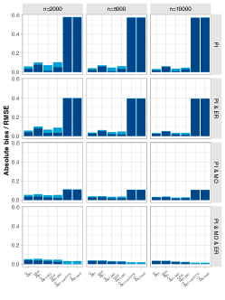
Figure 1: Estimators’ absolute bias and Root Mean Squared Error (RMSE) under misspecified parametric models across twelve scenario/sample size combinations.

Absolute bias is the darker portion of each bar; RMSE corresponds to the total bar size. Abbreviations: PI = Principal Ignorability (Scenario 1), PI & ER = Principal Ignorability and Exclusion Restriction (Scenario 2), PI & MO= Principal Ignorability and Monotonicity (Scenario 3), PI & ER & MO = Principal Ignorability, Exclusion Restriction and Monotonicity (Scenario 4).

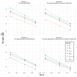
Figure 2: Estimators’ variance and rate of convergence under misspecified parametric models.

For each estimator/scenario combination, slopes describe rates of convergence (e.g., a slope of $-1/2$ points to a convergence speed of $\sqrt{n}$), while intercepts approximate the logarithm of asymptotic variances.

Table 1: Results of the simulation study for misspecified parametric models.

Scenario	Scenario 1: Principal ignorability			Scenario 2: Principal ignorability, and exclusion restriction			Scenario 3: Principal ignorability, and monotonicity			Scenario 4: Principal ignorability, exclusion restriction, and monotonicity
	$\operatorname{\mathbb{E}}[Y^{t=1}-Y^{t=0}]=-2.13\%$	$\operatorname{\mathbb{E}}[(Y^{s=a,z=0,t=1}-Y^{s=a,z=1,t=1})^{2}]=60.74\%$	$\operatorname{\mathbb{E}}[\rho_{c}(X)]=55.08\%$	$\operatorname{\mathbb{E}}[Y^{t=1}-Y^{t=0}]=-5.79\%$	$\operatorname{\mathbb{E}}[(Y^{s=a,z=0,t=1}-Y^{s=a,z=1,t=1})^{2}]=0$	$\operatorname{\mathbb{E}}[\rho_{c}(X)]=55.08\%$	$\operatorname{\mathbb{E}}[Y^{t=1}-Y^{t=0}]=13.54\%$	$\operatorname{\mathbb{E}}[(Y^{s=a,z=0,t=1}-Y^{s=a,z=1,t=1})^{2}]=60.74\%$	$\operatorname{\mathbb{E}}[\rho_{c}(X)]=65.30\%$	$\operatorname{\mathbb{E}}[Y^{t=1}-Y^{t=0}]=10.08\%$	$\operatorname{\mathbb{E}}[(Y^{s=a,z=0,t=1}-Y^{s=a,z=1,t=1})^{2}]=0$	$\operatorname{\mathbb{E}}[\rho_{c}(X)]=65.30\%$
	$\Delta=20.31\%$	$\operatorname{\mathbb{E}}[(Y^{s=n,z=1,t=0}-Y^{s=a,z=0,t=0})^{2}]=54.90\%$	$\operatorname{\mathbb{E}}[\rho_{d}(X)]=14.36\%$	$\Delta=20.31\%$	$\operatorname{\mathbb{E}}[(Y^{s=n,z=1,t=0}-Y^{s=a,z=0,t=0})^{2}]=0$	$\operatorname{\mathbb{E}}[\rho_{d}(X)]=14.36\%$	$\Delta=20.31\%$	$\operatorname{\mathbb{E}}[(Y^{s=n,z=1,t=0}-Y^{s=a,z=0,t=0})^{2}]=54.90\%$	$\operatorname{\mathbb{E}}[\rho_{d}(X)]=0$	$\Delta=20.31\%$	$\operatorname{\mathbb{E}}[(Y^{s=n,z=1,t=0}-Y^{s=a,z=0,t=0})^{2}]=0$	$\operatorname{\mathbb{E}}[\rho_{d}(X)]=0$
Estimator	Bias	Empirical SE	RMSE	Bias	Empirical SE	RMSE	Bias	Empirical SE	RMSE	Bias	Empirical SE	RMSE
$n=2000$
$\widehat{\Delta}_{PI}$	-3.27%	4.88%	5.88%	-3.97%	4.01%	5.64%	-3.46%	4.13%	5.39%	-4.06%	3.19%	5.16%
$\widehat{\Delta}_{PI}^{ER}$	-7.63%	6.51%	10.03%	-7.93%	6.12%	10.02%	-3.62%	4.88%	6.08%	-3.59%	4.23%	5.55%
$\widehat{\Delta}_{PI,MO}$	-1.17%	7.04%	7.14%	-3.09%	5.86%	6.63%	-2.67%	4.35%	5.10%	-3.13%	3.38%	4.60%
$\widehat{\Delta}_{PI,MO}^{ER}$	-4.97%	8.94%	10.23%	-3.37%	8.12%	8.80%	-2.12%	4.92%	5.36%	-2.25%	4.01%	4.59%
$\widehat{\Delta}_{IV\,matching}$	57.57%	7.17%	58.01%	39.55%	6.56%	40.09%	10.78%	3.46%	11.32%	0.13%	3.10%	3.10%
$\widehat{\Delta}_{IV\,wald}$	57.52%	7.09%	57.96%	39.53%	6.53%	40.07%	10.76%	3.41%	11.29%	0.12%	3.08%	3.09%
$n=5000$
$\widehat{\Delta}_{PI}$	-2.18%	3.38%	4.02%	-2.64%	2.58%	3.69%	-2.68%	2.78%	3.86%	-3.12%	2.14%	3.78%
$\widehat{\Delta}_{PI}^{ER}$	-5.71%	4.14%	7.05%	-5.00%	3.82%	6.29%	-2.89%	2.97%	4.14%	-3.00%	2.38%	3.83%
$\widehat{\Delta}_{PI,MO}$	-0.73%	4.60%	4.65%	-1.82%	3.79%	4.21%	-1.71%	2.88%	3.35%	-2.25%	2.21%	3.16%
$\widehat{\Delta}_{PI,MO}^{ER}$	-3.34%	5.30%	6.27%	-1.64%	4.47%	4.77%	-2.00%	3.02%	3.62%	-1.76%	2.38%	2.97%
$\widehat{\Delta}_{IV\,matching}$	57.29%	4.59%	57.47%	39.36%	4.11%	39.57%	10.64%	2.12%	10.84%	0.02%	1.98%	1.98%
$\widehat{\Delta}_{IV\,wald}$	57.28%	4.56%	57.46%	39.36%	4.08%	39.57%	10.64%	2.11%	10.85%	0.03%	1.97%	1.97%
$n=10000$
$\widehat{\Delta}_{PI}$	-1.78%	2.51%	3.08%	-2.42%	1.97%	3.12%	-2.58%	1.99%	3.25%	-3.06%	1.55%	3.43%
$\widehat{\Delta}_{PI}^{ER}$	-5.31%	3.09%	6.14%	-4.52%	2.59%	5.21%	-2.92%	2.08%	3.59%	-3.05%	1.77%	3.52%
$\widehat{\Delta}_{PI,MO}$	-0.91%	3.32%	3.44%	-1.92%	2.49%	3.15%	-1.60%	2.05%	2.61%	-2.15%	1.61%	2.68%
$\widehat{\Delta}_{PI,MO}^{ER}$	-2.77%	3.57%	4.52%	-1.27%	3.04%	3.30%	-1.96%	2.07%	2.85%	-1.61%	1.65%	2.30%
$\widehat{\Delta}_{IV\,matching}$	57.21%	3.27%	57.31%	39.25%	2.94%	39.36%	10.58%	1.54%	10.70%	-0.02%	1.40%	1.40%
$\widehat{\Delta}_{IV\,wald}$	57.22%	3.26%	57.32%	39.26%	2.94%	39.37%	10.59%	1.53%	10.70%	-0.02%	1.40%	1.40%

6 Application on the Promotion of Breastfeeding Intervention Trial

6.1 Description

The Promotion of Breastfeeding Intervention Trial (PROBIT) was conducted to assess the effects of a breastfeeding promotion program on infant weight at three months (Kramer et al., 2001). The trial recruited mother-infant pairs from 31 Belarusian maternity hospitals and randomly assigned them to either the breastfeeding promotion program or standard care. For our experiments, we used the PROBITsim simulation learner (Goetghebeur et al., 2020), which is a publicly available, anonymized database that replicates data from the original trial. In our setting, the allocated treatment corresponds to an allocation to the breastfeeding promotion program (i.e., if so, we have $Z=1$), and the treatment effectively taken describes whether a participant attended that program (i.e., in that case, we have $T=1$). Our main outcome of interest is infant weight at three months, discretized at 6000g (i.e., $Y=1$ for weights greater than 6000g). Participants’ pre-randomization covariates (i.e, the variable $X$) comprise two categorical variables (location, education), four binary variables (maternal allergy, smoking status, child born by caesarian, sex of the child), and two continuous variables (mother’s age at randomization, birth weigh). Our objective is to estimate the CACE, which, in this context, represents the effect among those individuals who will attend the breastfeeding program when invited but not otherwise. We estimate the CACE using four estimators introduced in this paper: $\widehat{\Delta}_{PI}$, $\widehat{\Delta}_{PI}^{ER}$, $\widehat{\Delta}_{PI,MO}$, $\widehat{\Delta}_{PI,MO}^{ER}$ as well as two instrumental variable estimators: $\widehat{\Delta}_{IVwald}$ and $\widehat{\Delta}_{IV\,matching}$. We calculate 95% confidence intervals (95% CI) using the bootstrap with 999 replicates.

6.2 Results

The estimated average treatment effect of the allocation to the breastfeeding promotion program vs the allocation to standard care was 0.07; 95% CI [0.06 to 0.09]. Because 36% of participants allocated to the program did not attend it, this so-called intention to treat analysis may lead to underemphasizing the intrinsic effect of the breastfeeding promotion program on infant weight at three months. In fact, the calculation of the CACE with all six estimators showed estimates greater than the estimated average treatment effect (Figure 3). The instrumental variable estimators $\widehat{\Delta}_{IVwald}$ and $\widehat{\Delta}_{IV\,matching},$ which rely on the exclusion restriction and monotonicity assumptions, both yield CACE estimates of 0.11 with tight confidence intervals (95% CI [0.09 to 0.14] and [0.09 to 0.13] respectively). On the other hand, the estimators $\widehat{\Delta}_{PI}$, $\widehat{\Delta}_{PI}^{ER}$, $\widehat{\Delta}_{PI,MO}$, and $\widehat{\Delta}_{PI,MO}^{ER}$ leverage the principal ignorability assumption, and compared to instrumental variable estimators, yield greater CACE estimates with larger confidence intervals. As we have no apriori reason to believe that exclusion restriction or monotonicity assumptions hold for the PROBIT study, the estimate from the $\widehat{\Delta}_{PI}$ estimator (0.20; 95% CI [0.16 to 0.23]) may provide a more reliable evaluation of the intrinsic effect of the program. Furthermore, because all six estimators point to clinically meaningfull and statistically significant effects, we can reasonably conclude that, in compliers, the breastfeeding promotion program causes greater infant weight at three months.

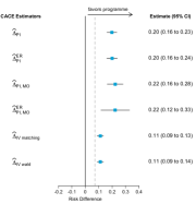
Figure 3: Estimation of the CACE for the Promotion of Breastfeeding Intervention Trial.

The gray dotted line indicates the estimated average treatment effect. Abbreviations: CACE = Complier Average Causal Effect.

7 Discussion

In this paper, we presented a probability model that defines the CACE from the perspective of mixtures of experts and supervised learning. We introduced four CACE estimators based on this model. These estimators leverage the information contained in the covariates $X$ through the principal ignorability assumption. Three of these estimators also utilize the common exclusion restriction and monotonicity assumptions, which help to reduce mean squared errors. Because of the generality of our causal framework, our estimators can be applied not only to randomized controlled trial data but also to observational data. Considering our framework, in step 2 of our estimation procedures, one may be tempted to estimate the conditional elementary potential outcome functions $Q_{c11}$ and $Q_{c00}$ together in a single mixture model. However, we have noticed that, with this approach, the parameters from the functions $Q_{c11}$ and $Q_{c00}$ would not be identifiable. On the other hand, we studied the properties of our proposed methodologies and proved that, under parametric assumptions, all the nuisance components are identifiable. Beyond the nonparametric extensions proposed in Appendix C, it is worth noting several other future directions for the work reported here. Our framework opens up the possibility of developing cross-validated CACE estimators, using machine learning to estimate each nuisance component on a different data split (Chernozhukov et al., 2018). This would in turn allow leveraging the use of influence functions (Hines et al., 2022) to develop more efficient (e.g., targeted learning) CACE estimators. Although we focused on binary and continuous outcomes, our methodology could, in principle, be readily extended to censored outcomes by using mixtures of survival models (Kuo and Peng, 2000). Finally, it would be worthwhile to extend the causal framework introduced in this paper to account for longitudinal measures of the treatment effectively taken.

Conflicts of interests

The authors have disclosed that they do not have any conflicts of interest related to this article.

Funding

RP acknowledges the support of the French Agence Nationale de la Recherche as part of the “Investissements d’avenir” program, reference ANR-19- P3IA-0001 (PRAIRIE 3IA Institute). FP acknowledges support from the French Agence Nationale de la Recherche through the project reference ANR-22-CPJ1-0047-01.

Author contributions

FG conceived the study. FG and CB wrote the codes and did the simulation and application analyses. FG and FP worked on the mathematical proofs. FG drafted the manuscript with inputs from CB, FP and RP. All the authors read the paper and suggested edits. RP supervised the project. FG and CB accessed and verified the data.

Supplementary Materials for “Estimating Complier Average Causal Effects with Mixtures of Experts”

Appendix A Summary of notations

Notation	Meaning
$X$	Baseline (i.e., pre-randomization) covariates
$Z$	Allocated binary treatment
$S_{c}$	Binary indicator whether a patient is a complier
$S_{a}$	Binary indicator whether a patient is an always-taker
$S_{n}$	Binary indicator whether a patient is a never-taker
$S_{d}$	Binary indicator whether a patient is a defier
$\boldsymbol{S}=(S_{c},S_{a},S_{n},S_{d})^{T}$	One-hot-encoded latent stratum of a patient
$\{T^{s=k}\}_{k\in\{c,a,n,d\}}$	Potential treatment under the stratum $k$
$T$	Treatment effectively taken
$\{Y^{s=k,z=l,t=m}\}_{k\in\{c,a,n,d\},l=\{0,1\},m=\{0,1\}}$	Elementary potential outcome
$\{Y^{t=m}\}_{m\in\{0,1\}}$	Potential outcome
$Y$	Observed outcome
$\Delta=\operatorname{\mathbb{E}}(Y^{t=1}-Y^{t=0}|S_{c}=1)$	Complier Average Causal Effect (CACE)
$\eta(x)=\operatorname{\mathbb{E}}(Z|X=x)$	Allocation ratio function
$e(x)=\operatorname{\mathbb{E}}(T|X=x)$	Standard propensity score
$\pi(x,z)=\operatorname{\mathbb{E}}(T|X=x,Z=z)$	Propensity score adaptation in the context of imperfect compliance
$\rho_{k}(x)=\operatorname{\mathbb{E}}(S_{k}|X=x)$	Probability functions that a patient with covariates $x$ is in the stratum $k$
$\mu_{k}(z)=\operatorname{\mathbb{E}}(T^{s=k}|Z=z)$	Known expert from a mixture of expert model
$P_{klm}(x)=\operatorname{\mathbb{E}}(S_{k}|Z=l,T=m,X=x)$	Probability functions that a patient with allocated treatment $l$,
	treatment taken $m$, and covariates $x$ is in the stratum $k$
$q_{lm}(x)=\operatorname{\mathbb{E}}(Y|Z=l,T=m,X=x)$	Conditional observed outcome functions
$Q_{klm}(x)=\operatorname{\mathbb{E}}(Y^{s=k,z=l,t=m}|X=x)$	Conditional elementary potential outcome functions
$P_{k\cdot m}(x)=\operatorname{\mathbb{E}}(S_{k}|T=m,X=x)$	Probability functions that a patient with treatment taken $m$,
	and covariates $x$ is in the stratum $k$
$q_{\cdot m}(x)=\operatorname{\mathbb{E}}(Y|T=m,X=x)$	Conditional observed outcome functions, irrespective of $Z$
$Q_{k}(x)=\operatorname{\mathbb{E}}(Y^{s=k}|X=x)$	Conditional potential outcome functions under exclusion restriction
$\mathcal{X}=\mathbb{R}^{d}$	Space of covariates
$\mathcal{Z}=\{0,1\}$	Space of allocated treatments
$\mathcal{P}$	Probability distribution of the experiment
$k\in\{c,a,n,d\}$	Index for a particular stratum
$l\in\{0,1\}$	Index for a particular allocated treatment
$m\in\{0,1\}$	Index for a particular treatment taken
$\widehat{\Delta}_{PI}$	CACE estimator assuming principal ignorability
$\widehat{\Delta}_{PI}^{ER}$	CACE estimator assuming principal ignorability and exclusion restriction
$\widehat{\Delta}_{PI,MO}$	CACE estimator assuming principal ignorability and monotonicity
$\widehat{\Delta}_{PI,MO}^{ER}$	CACE estimator assuming principal ignorability, exclusion restriction and monotonicity
$\widehat{\Delta}_{IV\,matching}$	CACE instrumental variable estimator using matching
$\widehat{\Delta}_{IV\,wald}$	Standard CACE instrumental variable estimator

Appendix B Proofs

B.1 Proof of Lemma 1

Proof B.13.

$$\Delta \operatorname*{\stackrel{{\scriptstyle\text{def}}}{{=}}}\operatorname{\mathbb{E}}[Y^{t=1}-Y^{t=0}|S_{c}=1]$$

$$=\operatorname{\mathbb{E}}[Y^{s=c,z=1,t=1}-Y^{s=c,z=0,t=0}|S_{c}=1]$$

$$=\operatorname{\mathbb{E}}\Big{[}\operatorname{\mathbb{E}}\big{(}Y^{s=c,z=1,t=1}-Y^{s=c,z=0,t=0}|X,S_{c}\big{)}|S_{c}=1\Big{]}$$

$$=\operatorname{\mathbb{E}}\Big{[}\operatorname{\mathbb{E}}\big{(}Y^{s=c,z=1,t=1}-Y^{s=c,z=0,t=0}|X\big{)}|S_{c}=1\Big{]}$$ (Assumption 3(i))

$$=\operatorname{\mathbb{E}}\Big{[}\operatorname{\mathbb{E}}(Y^{s=c,z=1,t=1}|X)-\operatorname{\mathbb{E}}(Y^{s=c,z=0,t=0}|X)|S_{c}=1\Big{]}$$

$$=\operatorname{\mathbb{E}}\Big{[}Q_{c11}(X)-Q_{c00}(X)|S_{c}=1\Big{]}$$

$$=\int_{\mathcal{X}}\big{\{}Q_{c11}(x)-Q_{c00}(x)\big{\}}p_{X|S_{c}}(x|1)dx$$

$$=\int_{\mathcal{X}}\big{\{}Q_{c11}(x)-Q_{c00}(x)\big{\}}\frac{p_{S_{c}|X}(1|x)}{p_{S_{c}}(1)}p_{X}(x)dx$$

$$=\operatorname{\mathbb{E}}\Bigg{[}\big{\{}Q_{c11}(X)-Q_{c00}(X)\big{\}}\frac{\operatorname{\mathbb{E}}(S_{c}|X)}{\operatorname{\mathbb{E}}(S_{c})}\Bigg{]}$$

$$=\operatorname{\mathbb{E}}\Big{[}\big{\{}Q_{c11}(X)-Q_{c00}(X)\big{\}}\operatorname{\mathbb{E}}(S_{c}|X)\Big{]}/\operatorname{\mathbb{E}}(S_{c})$$

$$=\operatorname{\mathbb{E}}\Big{[}\big{\{}Q_{c11}(X)-Q_{c00}(X)\big{\}}\operatorname{\mathbb{E}}(S_{c}|X)\Big{]}/\operatorname{\mathbb{E}}[\operatorname{\mathbb{E}}(S_{c}|X)]$$

$$=\operatorname{\mathbb{E}}\Big{[}\big{\{}Q_{c11}(X)-Q_{c00}(X)\big{\}}\rho_{c}(X)\Big{]}/\operatorname{\mathbb{E}}[\rho_{c}(X)]$$

Assumption 4 guarantees that the conditioning on $\{S_{c}=1\}$ is well-defined, and that $\operatorname{\mathbb{E}}[p_{c}(X)]\neq 0$.

B.2 Proof of Lemma 2

Proof B.14.

$$\pi(X,Z) \operatorname*{\stackrel{{\scriptstyle\text{def}}}{{=}}}\operatorname{\mathbb{E}}(T|X,Z)$$

$$=\operatorname{\mathbb{E}}(S_{c}T^{s=c}+S_{a}T^{s=a}+S_{n}T^{s=n}+S_{d}T^{s=d}|X,Z)$$ (Definition 1)

$$=\operatorname{\mathbb{E}}(S_{c}Z+S_{a}\times 1+S_{n}\times 0+S_{d}(1-Z)|X,Z)$$

$$=Z\operatorname{\mathbb{E}}(S_{c}|X,Z)+1\times\operatorname{\mathbb{E}}(S_{a}|X,Z)+0\times\operatorname{\mathbb{E}}(S_{n}|X,Z)+(1-Z)\operatorname{\mathbb{E}}(S_{d}|X,Z)$$

$$=Z\operatorname{\mathbb{E}}(S_{c}|X)+1\times\operatorname{\mathbb{E}}(S_{a}|X)+0\times\operatorname{\mathbb{E}}(S_{n}|X)+(1-Z)\operatorname{\mathbb{E}}(S_{d}|X)$$ (Asm. 3(i))

$$=\operatorname{\mathbb{E}}(Z|Z)\operatorname{\mathbb{E}}(S_{c}|X)+\operatorname{\mathbb{E}}(1|Z)\operatorname{\mathbb{E}}(S_{a}|X)+\operatorname{\mathbb{E}}(0|Z)\operatorname{\mathbb{E}}(S_{n}|X)+\operatorname{\mathbb{E}}(1-Z|Z)\operatorname{\mathbb{E}}(S_{d}|X)$$

$$=\operatorname{\mathbb{E}}(S_{c}|X)\operatorname{\mathbb{E}}(T^{s=c}|Z)+\operatorname{\mathbb{E}}(S_{a}|X)\operatorname{\mathbb{E}}(T^{s=a}|Z)+\operatorname{\mathbb{E}}(S_{n}|X)\operatorname{\mathbb{E}}(T^{s=n}|Z)+\operatorname{\mathbb{E}}(S_{d}|X)\operatorname{\mathbb{E}}(T^{s=d}|Z)$$

$$=\sum_{k\in\{c,a,n,d\}}\rho_{k}(X)\mu_{k}(Z)$$

Assumption 1 guarantees that the conditioning on $\{X,Z\}$ is well-defined.

B.3 Proof of Lemma 3

Proof B.15.

$$q_{11}(X)\operatorname*{\stackrel{{\scriptstyle\text{def}}}{{=}}} \operatorname{\mathbb{E}}(Y|Z=1,T=1,X)$$

$$= \operatorname{\mathbb{E}}(TY^{t=1}+(1-T)Y^{t=0}|Z=1,T=1,X)$$ (Assumption 2)

$$= \operatorname{\mathbb{E}}(Y^{t=1}|Z=1,T=1,X)$$

$$= \operatorname{\mathbb{E}}(S_{c}Y^{s=c,z=1,t=1}+S_{a}Y^{s=a,z=1,t=1}|Z=1,T=1,X)$$ (Definition 2)

$$= \operatorname{\mathbb{E}}(S_{c}|Z=1,T=1,X)\operatorname{\mathbb{E}}(Y^{s=c,z=1,t=1}|Z=1,T=1,X)$$

$$+\operatorname{\mathbb{E}}(S_{a}|Z=1,T=1,X)\operatorname{\mathbb{E}}(Y^{s=a,z=1,t=1}|Z=1,T=1,X)$$ (2)

$$= \operatorname{\mathbb{E}}(S_{c}|Z=1,T=1,X)\operatorname{\mathbb{E}}(Y^{s=c,z=1,t=1}|X)$$

$$+\operatorname{\mathbb{E}}(S_{a}|Z=1,T=1,X)\operatorname{\mathbb{E}}(Y^{s=a,z=1,t=1}|X)$$ (3)

$$= P_{c11}(X)Q_{c11}(X)+P_{a11}(X)Q_{a11}(X)$$

Assumptions 1, 3(i), and 4 guarantees that the conditioning on $\{Z=1,T=1,X\}$ is well-defined. The equality in (2) rely on Assumption 3(ii). The equalities in (2) and (3) rely on the fact that the extra conditioning on $\{Z=1,T=1\}$ does not open a backdoor path (this can be verified by appealing to a d-separation argument on the graph given in Appendix B.7). The proof for the $q_{00}(X)$ formula follows a similar argument.

B.4 Proof of Lemma 4

Proof B.16.

$$P_{c11}(X) \operatorname*{\stackrel{{\scriptstyle\text{def}}}{{=}}}\operatorname{\mathbb{E}}(S_{c}|Z=1,T=1,X)$$

$$=\operatorname{\mathbb{P}}(S_{c}=1|Z=1,T=1,X)$$

$$=\operatorname{\mathbb{P}}(T=1|S_{c}=1,Z=1,X)\frac{\operatorname{\mathbb{P}}(S_{c}=1|Z=1,X)}{\operatorname{\mathbb{P}}(T=1|Z=1,X)}$$

$$=\operatorname{\mathbb{E}}(S_{c}Z+S_{a}+S_{d}(1-Z)|S_{c}=1,Z=1,X)\frac{\operatorname{\mathbb{P}}(S_{c}=1|Z=1,X)}{\operatorname{\mathbb{P}}(T=1|Z=1,X)}$$ (Def. 1)

$$=\frac{\operatorname{\mathbb{P}}(S_{c}=1|Z=1,X)}{\operatorname{\mathbb{P}}(T=1|Z=1,X)}$$

$$=\frac{\operatorname{\mathbb{P}}(S_{c}=1|X)}{\operatorname{\mathbb{E}}(T|Z=1,X)}$$ (Assumption 3(i))

$$=\frac{\operatorname{\mathbb{E}}(S_{c}|X)}{\operatorname{\mathbb{E}}(S_{c}|Z=1,X)+\operatorname{\mathbb{E}}(S_{a}|Z=1,X)}$$ (Definition 1)

$$=\frac{\operatorname{\mathbb{E}}(S_{c}|X)}{\operatorname{\mathbb{E}}(S_{c}|X)+\operatorname{\mathbb{E}}(S_{a}|X)}$$ (Assumption 3(i))

$$=\rho_{c}(X)/\{\rho_{c}(X)+\rho_{a}(X)\}.$$

Assumptions 1, 3(i), and 4 guarantees that the conditioning on $\{Z=1,T=1,X\}$ is well-defined. The proof for the $P_{a11}$, $P_{c00}$, and $P_{n00}$ formulas follows a similar argument.

B.5 Proof of Lemma 5

Proof B.17.

$$q_{\cdot 1}(X)\operatorname*{\stackrel{{\scriptstyle\text{def}}}{{=}}} \operatorname{\mathbb{E}}(Y|T=1,X)$$

$$= \operatorname{\mathbb{E}}(TY^{t=1}+(1-T)Y^{t=0}|T=1,X)$$ (Assumption 2)

$$= \operatorname{\mathbb{E}}(Y^{t=1}|T=1,X)$$

$$= \operatorname{\mathbb{E}}(S_{c}Y^{s=c,z=1,t=1}+S_{a}Y^{s=a}+S_{d}Y^{s=c,z=0,t=1}|T=1,X)$$ (Assumption 5)

$$= \operatorname{\mathbb{E}}(S_{c}|T=1,X)\operatorname{\mathbb{E}}(Y^{s=c,z=1,t=1}|T=1,X)$$ (4)

$$+\operatorname{\mathbb{E}}(S_{a}|T=1,X)\operatorname{\mathbb{E}}(Y^{s=a}|T=1,X)$$

$$+\operatorname{\mathbb{E}}(S_{d}|T=1,X)\operatorname{\mathbb{E}}(Y^{s=c,z=0,t=1}|T=1,X)$$

$$= \operatorname{\mathbb{E}}(S_{c}|T=1,X)\operatorname{\mathbb{E}}(Y^{s=c,z=1,t=1}|X)$$ (5)

$$+\operatorname{\mathbb{E}}(S_{a}|T=1,X)\operatorname{\mathbb{E}}(Y^{s=a}|X)$$

$$+\operatorname{\mathbb{E}}(S_{d}|T=1,X)\operatorname{\mathbb{E}}(Y^{s=c,z=0,t=1}|X)$$

$$= P_{c\cdot 1}(X)Q_{c11}(X)+P_{a\cdot 1}(X)Q_{a}(X)+P_{d\cdot 1}(X)Q_{d01}(X)$$

Assumptions 1 and 4 guarantees that the conditioning on $\{T=1,X\}$ is well-defined. The equality in (4) rely on Assumption 3(ii). The equalities in (4) and (5) rely on the fact that the extra conditioning on $T=1$ does not open a backdoor path (this can be verified by appealing to a d-separation argument on the graph given in subsection B.7). The proof for the $q_{\cdot 0}(X)$ formula follows a similar argument.

B.6 Proof of Lemma 6

Proof B.18.

$$P_{c\cdot 1}(X)\operatorname*{\stackrel{{\scriptstyle\text{def}}}{{=}}} \operatorname{\mathbb{E}}(S_{c}|T=1,X)$$

$$= \operatorname{\mathbb{P}}(Z=0|T=1,X)\overbrace{\operatorname{\mathbb{P}}(S_{c}=1|Z=0,T=1,X)}^{=0}$$

$$+\operatorname{\mathbb{P}}(Z=1|T=1,X)\operatorname{\mathbb{P}}(S_{c}=1|Z=1,T=1,X)$$

$$= \operatorname{\mathbb{P}}(Z=1|T=1,X)P_{c11}(X)$$

$$= \frac{\operatorname{\mathbb{P}}(Z=1|X)}{\operatorname{\mathbb{P}}(T=1|X)}\operatorname{\mathbb{P}}(T=1|Z=1,X)P_{c11}(X)$$

$$= \frac{\eta(X)}{e(X)}\operatorname{\mathbb{E}}(S_{c}Z+S_{a}+S_{d}(1-Z)|Z=1,X)P_{c11}(X)$$ (Definition 1)

$$= \frac{\eta(X)}{e(X)}\big{\{}\operatorname{\mathbb{E}}(S_{c}|Z=1,X)+\operatorname{\mathbb{E}}(S_{a}|Z=1,X)\big{\}}P_{c11}(X)$$

$$= \frac{\eta(X)}{e(X)}\big{\{}\operatorname{\mathbb{E}}(S_{c}|X)+\operatorname{\mathbb{E}}(S_{a}|X)\big{\}}P_{c11}(X)$$ (Assumption 3(i))

$$= \frac{\eta(X)}{e(X)}\big{\{}\rho_{c}(X)+\rho_{a}(X)\big{\}}\frac{\rho_{c}(X)}{\rho_{c}(X)+\rho_{a}(X)}$$ (Lemma 4)

$$= \frac{\eta(X)}{e(X)}\rho_{c}(X)$$

Assumptions 1 and 4 guarantees that the conditioning on $\{T=1,X\}$ is well-defined. The proofs for the $P_{a\cdot 1}(X)$, $P_{d\cdot 1}(X)$, $P_{c\cdot 0}(X)$, $P_{n\cdot 0}(X)$, and $P_{d\cdot 0}(X)$ formulas follow similar arguments. The standard propensity score can be further represented as

$$e(X)\operatorname*{\stackrel{{\scriptstyle\text{def}}}{{=}}} \operatorname{\mathbb{E}}(T|X)$$

$$= \operatorname{\mathbb{E}}(S_{c}Z+S_{a}+S_{d}(1-Z)|X)$$

$$= \operatorname{\mathbb{E}}(S_{c}|X)\operatorname{\mathbb{E}}(Z|X)+\operatorname{\mathbb{E}}(S_{a}|X)+\operatorname{\mathbb{E}}(S_{d}|X)\operatorname{\mathbb{E}}(1-Z|X)$$ (Assumption 3(i))

$$= \rho_{c}(X)\eta(X)+\rho_{a}(X)+\rho_{d}(X)\{1-\eta(X)\}.$$

B.7 Probabilistic graphical model

Below, we provide the probabilistic graphical model corresponding to the data generating mechanism described in section 2. Conditional independences between variables can be read from this diagram using the rules of d-separation. For clarity we use random vector notation

$$\boldsymbol{Y^{s,z,t}}=( Y^{s=c,z=1,t=1},Y^{s=a,z=1,t=1},Y^{s=a,z=0,t=1},Y^{s=d,z=0,t=1},$$

$$\quad Y^{s=c,z=0,t=0},Y^{s=n,z=1,t=0},Y^{s=n,z=0,t=0},Y^{s=d,z=1,t=0})^{T}$$

and $\boldsymbol{Y^{t}}=(Y^{t=1},Y^{t=0})^{T}.$

Appendix C EM algorithms

All EM algorithms in this section are adaptations of the algorithm provided in Jordan and Jacobs (1994), based on the description from Xu and Jordan (1993). Algorithms C.2, C.3, C.5, C.6, C.7, C.8, and C.10 take a data subset as input. To avoid clutter, we drop subscripts of the form $(-)_{i:Z_{i}=l,T_{i}=l}$ in these algorithms. However, as a reminder of data subsetting, we note sums over $n^{\prime}$ elements rather than $n$.

Algorithm C.1 The EM procedure for estimating $\rho_{s}(\cdot;\delta_{s})$ where $s\in\{c,a,n,d\}$.

Data $(X_{i}^{\rho},Z_{i},T_{i})_{1\leq i\leq n}$ where $X_{i}^{\rho}$ is a relevant subset of the variables contained in $X_{i}$.

the prior probabilities associated with the nodes of the tree as

$$g_{c,i}\leftarrow 1/4,\quad g_{a,i}\leftarrow 1/4,\quad g_{n,i}\leftarrow 1/4,\quad\text{and}\quad g_{d,i}\leftarrow 1/4.$$

individual contributions to each expert’s likelihood as

$$L_{c,i}\leftarrow Z_{i}T_{i}+(1-Z_{i})(1-T_{i})$$

$$L_{a,i}\leftarrow T_{i}$$

$$L_{n,i}\leftarrow 1-T_{i}$$

$$L_{d,i}\leftarrow Z_{i}(1-T_{i})+(1-Z_{i})T_{i}$$

until convergence on the parameters $\delta=(\delta_{c}^{T},\delta_{a}^{T},\delta_{n}^{T},\delta_{d}^{T})^{T}$:

Compute the posterior probabilities associated with the nodes of the tree as $\triangleright$ E-step

$$h_{c,i}\leftarrow g_{c,i}L_{c,i}/\sum_{s\in\{c,a,n,d\}}g_{s,i}L_{s,i}$$

$$h_{a,i}\leftarrow g_{a,i}L_{a,i}/\sum_{s\in\{c,a,n,d\}}g_{s,i}L_{s,i}$$

$$h_{n,i}\leftarrow g_{n,i}L_{n,i}/\sum_{s\in\{c,a,n,d\}}g_{s,i}L_{s,i}$$

$$h_{d,i}\leftarrow g_{d,i}L_{d,i}/\sum_{s\in\{c,a,n,d\}}g_{s,i}L_{s,i}$$

For the gating network $\rho(\cdot)$ estimate parameters $\delta$ by solving the IRLS problem$\triangleright$ M-step

$$\delta\leftarrow\operatorname*{arg\,max}\limits_{\delta}\sum_{i=1}^{n}\sum_{s\in\{c,a,n,d\}}h_{s,i}\ln{\Big{(}\exp{\delta_{s}^{T}X_{i}^{\rho}}/\sum_{k\in\{c,a,n,d\}}\exp{\delta_{k}^{T}X_{i}^{\rho}}\Big{)}}$$

    as a multinomial logistic regression with features $(X_{i}^{\rho})_{1\leq i\leq n}$,

    and targets $(h_{c,i},h_{a,i},h_{n,i},h_{d,i})_{1\leq i\leq n}.$

Update the prior probabilities associated with the nodes of the tree as

$$g_{c,i}\leftarrow\exp{\delta_{c}^{T}X_{i}^{\rho}}/\sum_{k\in\{c,a,n,d\}}\exp{\delta_{k}^{T}X_{i}^{\rho}}$$

$$g_{a,i}\leftarrow\exp{\delta_{a}^{T}X_{i}^{\rho}}/\sum_{k\in\{c,a,n,d\}}\exp{\delta_{k}^{T}X_{i}^{\rho}}$$

$$g_{n,i}\leftarrow\exp{\delta_{n}^{T}X_{i}^{\rho}}/\sum_{k\in\{c,a,n,d\}}\exp{\delta_{k}^{T}X_{i}^{\rho}}$$

$$g_{d,i}\leftarrow\exp{\delta_{d}^{T}X_{i}^{\rho}}/\sum_{k\in\{c,a,n,d\}}\exp{\delta_{k}^{T}X_{i}^{\rho}}$$

$\rho_{s}(x;\hat{\delta})=\exp{\delta_{s}^{T}x}/\sum_{k\in\{c,a,n,d\}}\exp{\delta_{k}^{T}x}.$

Algorithm C.2 The EM procedure for estimating $Q_{c}(\cdot;\zeta)$ when $Y$ is binary. Here, $Q_{c}$ denotes either $Q_{c11}$ or $Q_{c00}$ depending on the data subset considered.

Data $(X_{i}^{\zeta},Y_{i},P_{cll}(X_{i}))_{i:Z_{i}=l,T_{i}=l}$ where $l\in\{0,1\}$ and $X_{i}^{\zeta}$ is a relevant subset of the variables contained in $X_{i}.$

the prior probabilities associated with the nodes of the tree as

$$g_{c,i}\leftarrow P_{cll}(X_{i}),\quad g_{nc,i}\leftarrow 1-P_{cll}(X_{i}).$$

the parameters $(\zeta_{c},\zeta_{nc})$ of the experts $\big{(}Q_{c}(\cdot),Q_{nc}(\cdot)\big{)}$ at random e.g.,

$$\zeta_{c}\sim\mathcal{N}(0,D)\quad\zeta_{nc}\sim\mathcal{N}(0,D)$$

with $D$ a diagonal matrix.

individual predictions from the initiated expert networks $\big{(}Q_{c}(\cdot),Q_{nc}(\cdot)\big{)}$ as

$$Q_{c,i}\leftarrow\operatorname{expit}(\zeta_{c}^{T}X_{i}^{\zeta})\quad Q_{nc,i}\leftarrow\operatorname{expit}(\zeta_{nc}^{T}X_{i}^{\zeta})$$

until convergence on the parameters $\zeta=(\zeta_{c}^{T},\zeta_{nc}^{T})^{T}$:

Compute individual contributions to each expert’s likelihood as

$$L_{c,i}\leftarrow Q_{c,i}^{Y_{i}}(1-Q_{c,i})^{1-Y_{i}}$$

$$L_{nc,i}\leftarrow Q_{nc,i}^{Y_{i}}(1-Q_{nc,i})^{1-Y_{i}}$$

Compute the posterior probabilities associated with the nodes of the tree as $\triangleright$ E-step

$$h_{c,i}\leftarrow g_{c,i}L_{c,i}/\Big{(}g_{c,i}L_{c,i}+g_{nc,i}L_{nc,i}\Big{)}$$

$$h_{nc,i}\leftarrow 1-h_{nc,i}$$

For the expert network $Q_{c}(\cdot)$ estimate parameters $\zeta_{c}$ by solving the IRLS problem $\triangleright$ M-step

$$\zeta_{c}\leftarrow\operatorname*{arg\,max}\limits_{\zeta_{c}}\sum_{i=1}^{n^{\prime}}h_{c,i}\Big{[}Y_{i}\ln{\{\operatorname{expit}(\zeta_{c}^{T}X_{i}^{\zeta})\}}+(1-Y_{i})\ln{\{1-\operatorname{expit}(\zeta_{c}^{T}X_{i}^{\zeta})\}}\Big{]}$$

    as a weighted logistic regression with features $X_{i}^{\zeta}$, targets $Y_{i}$ and weights $h_{c,i}$.

For the expert network $Q_{nc}(\cdot)$ estimate parameters $\zeta_{nc}$ by solving the IRLS problem

$$\zeta_{nc}\leftarrow\operatorname*{arg\,max}\limits_{\zeta_{nc}}\sum_{i=1}^{n^{\prime}}h_{nc,i}\Big{[}Y_{i}\ln{\{\operatorname{expit}(\zeta_{nc}^{T}X_{i}^{\zeta})\}}+(1-Y_{i})\ln{\{1-\operatorname{expit}(\zeta_{nc}^{T}X_{i}^{\zeta})\}}\Big{]}$$

    as a weighted logistic regression with features $X_{i}^{\zeta}$, targets $Y_{i}$ and weights $h_{nc,i}$.

Update the predictions from the expert networks $\big{(}Q_{c}(\cdot),Q_{nc}(\cdot)\big{)}$ as

$$Q_{c,i}\leftarrow\operatorname{expit}(\zeta_{c}^{T}X_{i}^{\zeta})\quad Q_{nc,i}\leftarrow\operatorname{expit}(\zeta_{nc}^{T}X_{i}^{\zeta})$$

$Q_{c}(x;\hat{\zeta})=\operatorname{expit}{(\zeta_{c}^{T}x)}$

Algorithm C.3 The EM procedure for estimating $Q_{c}(\cdot;\zeta)$ when $Y$ is continuous. Here, $Q_{c}$ denotes either $Q_{c11}$ or $Q_{c00}$ depending on the data subset considered.

Data $(X_{i}^{\zeta},Y_{i},P_{cll}(X_{i}))_{i:Z_{i}=l,T_{i}=l}$ where $l\in\{0,1\}$ and $d$-dimensional $X_{i}^{\zeta}$ is a relevant subset of the variables contained in $X_{i}.$

the prior probabilities associated with the nodes of the tree as

$$g_{c,i}\leftarrow P_{cll}(X_{i}),\quad g_{nc,i}\leftarrow 1-P_{cll}(X_{i}).$$

the parameters $\Big{(}(\zeta_{c},\sigma_{c}^{2}),(\zeta_{nc},\sigma_{nc}^{2})\Big{)}$ of the experts $\big{(}Q_{c}(\cdot),Q_{nc}(\cdot)\big{)}$ at random e.g.,

$$\zeta_{c}\sim\mathcal{N}(0,D)\quad\sigma_{c}^{2}\leftarrow 1$$

$$\zeta_{nc}\sim\mathcal{N}(0,D)\quad\sigma_{nc}^{2}\leftarrow 1$$

with $D$ a diagonal matrix.

individual predictions from the initiated expert networks $\big{(}Q_{c}(\cdot),Q_{nc}(\cdot)\big{)}$ as

$$Q_{c,i}\leftarrow\zeta_{c}^{T}X_{i}^{\zeta}\quad Q_{nc,i}\leftarrow\zeta_{nc}^{T}X_{i}^{\zeta}$$

until convergence on the parameters $\zeta=(\zeta_{c}^{T},\zeta_{nc}^{T})^{T}$:

Compute individual contributions to each expert’s likelihood as

$$L_{c,i}\leftarrow\mathcal{N}_{\mathcal{L}}(Y_{i}|\mu=Q_{c,i},\sigma^{2}=\sigma_{c}^{2}) L_{nc,i}\leftarrow\mathcal{N}_{\mathcal{L}}(Y_{i}|\mu=Q_{nc,i},\sigma^{2}=\sigma_{nc}^{2})$$

Compute the posterior probabilities associated with the nodes of the tree as $\triangleright$ E-step

$$h_{c,i}\leftarrow g_{c,i}L_{c,i}/\Big{(}g_{c,i}L_{c,i}+g_{nc,i}L_{nc,i}\Big{)} h_{nc,i}\leftarrow 1-h_{nc,i}$$

For the expert network $Q_{c}(\cdot)$ estimate parameters $\zeta_{c}$ by solving the

    weighted least-squares problem $\triangleright$ M-step

$$\zeta_{c}\leftarrow\operatorname*{arg\,min}\limits_{\zeta_{c}}\sum_{i=1}^{n^{\prime}}h_{c,i}\big{(}Y_{i}-\zeta_{c}^{T}X_{i}^{\zeta}\big{)}^{2}$$

    as a weighted linear regression with features $X_{i}^{\zeta}$, targets $Y_{i}$ and weights $h_{c,i}$.

For the expert network $Q_{nc}(\cdot)$ estimate parameters $\zeta_{nc}$ by solving the

    weighted least-squares problem

$$\zeta_{nc}\leftarrow\operatorname*{arg\,min}\limits_{\zeta_{nc}}\sum_{i=1}^{n^{\prime}}h_{nc,i}\big{(}Y_{i}-\zeta_{nc}^{T}X_{i}^{\zeta}\big{)}^{2}$$

    as a weighted linear regression with features $X_{i}^{\zeta}$, targets $Y_{i}$ and weights $h_{nc,i}$.

Update the variance parameter for each expert $\big{(}Q_{c}(\cdot),Q_{nc}(\cdot)\big{)}$ as

$$\sigma_{c}^{2}\leftarrow\frac{1}{n^{\prime}-d}\sum_{i=1}^{n^{\prime}}h_{c,i}\big{(}Y_{i}-\zeta_{c}^{T}X_{i}^{\zeta}\big{)}^{2},\quad\sigma_{nc}^{2}\leftarrow\frac{1}{n^{\prime}-d}\sum_{i=1}^{n^{\prime}}h_{nc,i}\big{(}Y_{i}-\zeta_{nc}^{T}X_{i}^{\zeta}\big{)}^{2}$$

Update the predictions from the expert networks $\big{(}Q_{c}(\cdot),Q_{nc}(\cdot)\big{)}$ as

$$Q_{c,i}\leftarrow\zeta_{c}^{T}X_{i}^{\zeta}\quad Q_{nc,i}\leftarrow\zeta_{nc}^{T}X_{i}^{\zeta}$$

$Q_{c}(x;\hat{\zeta})=\zeta_{c}^{T}x$

Algorithm C.4 The nonparametric EM-like procedure for estimating $\rho_{s}(\cdot)$ where $s\in\{c,a,n,d\}$.

Data $(X_{i}^{\rho},Z_{i},T_{i})_{1\leq i\leq n}$ where $X_{i}^{\rho}$ is a relevant subset of the variables contained in $X_{i}$.

the prior probabilities associated with the nodes of the tree as

$$g_{c,i}\leftarrow 1/4,\quad g_{a,i}\leftarrow 1/4,\quad g_{n,i}\leftarrow 1/4,\quad\text{and}\quad g_{d,i}\leftarrow 1/4.$$

individual contributions to each expert’s likelihood as

$$L_{c,i}\leftarrow Z_{i}T_{i}+(1-Z_{i})(1-T_{i})$$

$$L_{a,i}\leftarrow T_{i}$$

$$L_{n,i}\leftarrow 1-T_{i}$$

$$L_{d,i}\leftarrow Z_{i}(1-T_{i})+(1-Z_{i})T_{i}$$

until convergence:

Compute the posterior probabilities associated with the nodes of the tree as $\triangleright$ E-step

$$h_{c,i}\leftarrow g_{c,i}L_{c,i}/\sum_{s\in\{c,a,n,d\}}g_{s,i}L_{s,i}$$

$$h_{a,i}\leftarrow g_{a,i}L_{a,i}/\sum_{s\in\{c,a,n,d\}}g_{s,i}L_{s,i}$$

$$h_{n,i}\leftarrow g_{n,i}L_{n,i}/\sum_{s\in\{c,a,n,d\}}g_{s,i}L_{s,i}$$

$$h_{d,i}\leftarrow g_{d,i}L_{d,i}/\sum_{s\in\{c,a,n,d\}}g_{s,i}L_{s,i}$$

For the gating network fit $\hat{\rho}_{s}(\cdot),s\in\{c,a,n,d\}$ as a multiclass classification $\triangleright$ M-step

    problem with features $(X_{i}^{\hat{\rho}})_{1\leq i\leq n}$, and targets $(h_{c,i},h_{a,i},h_{n,i},h_{d,i})_{1\leq i\leq n}.$

Update the prior probabilities associated with the nodes of the tree as

$$g_{c,i}\leftarrow\hat{\rho}_{c}(X_{i}\rho),\quad g_{a,i}\leftarrow\hat{\rho}_{a}(X_{i}\rho),\quad g_{n,i}\leftarrow\hat{\rho}_{n}(X_{i}\rho),\quad g_{d,i}\leftarrow\hat{\rho}_{d}(X_{i}\rho)$$

$\hat{\rho}_{c}(\cdot)$

Algorithm C.5 The nonparametric EM-like procedure for estimating $Q_{c}(\cdot;\zeta)$ when $Y$ is binary. Here, $Q_{c}$ denotes either $Q_{c11}$ or $Q_{c00}$ depending on the data subset considered.

Data $(X_{i}^{\zeta},Y_{i},P_{cll}(X_{i}))_{i:Z_{i}=l,T_{i}=l}$ where $l\in\{0,1\}$ and $X_{i}^{\zeta}$ is a relevant subset of the variables contained in $X_{i}.$

the prior probabilities associated with the nodes of the tree as

$$g_{c,i}\leftarrow P_{cll}(X_{i}),\quad g_{nc,i}\leftarrow 1-P_{cll}(X_{i}).$$

the individual predictions from the expert networks $\big{(}Q_{c}(\cdot),Q_{nc}(\cdot)\big{)}$ as

$$Q_{c,i}\sim\mathcal{U}_{[0,1]}\quad Q_{nc,i}\sim\mathcal{U}_{[0,1]}$$

until convergence:

Compute individual contributions to each expert’s likelihood as

$$L_{c,i}\leftarrow Q_{c,i}^{Y_{i}}(1-Q_{c,i})^{1-Y_{i}}$$

$$L_{nc,i}\leftarrow Q_{nc,i}^{Y_{i}}(1-Q_{nc,i})^{1-Y_{i}}$$

Compute the posterior probabilities associated with the nodes of the tree as $\triangleright$ E-step

$$h_{c,i}\leftarrow g_{c,i}L_{c,i}/\Big{(}g_{c,i}L_{c,i}+g_{nc,i}L_{nc,i}\Big{)}$$

$$h_{nc,i}\leftarrow 1-h_{nc,i}$$

For the expert network $Q_{c}(\cdot)$ fit $\hat{Q}_{c}(\cdot)$ via a weighted nonparametric classifier $\triangleright$ M-step

    with features $X_{i}^{\zeta}$, targets $Y_{i}$ and weights $h_{c,i}$.

For the expert network $Q_{nc}(\cdot)$ fit $\hat{Q}_{nc}(\cdot)$ via a weighted nonparametric classifier

    with features $X_{i}^{\zeta}$, targets $Y_{i}$ and weights $h_{nc,i}$.

Update the predictions from the expert networks $\big{(}Q_{c}(\cdot),Q_{nc}(\cdot)\big{)}$ as

$$Q_{c,i}\leftarrow\hat{Q}_{c}(X_{i}^{\zeta})\quad Q_{nc,i}\leftarrow\hat{Q}_{nc}(X_{i}^{\zeta})$$

$\hat{Q}_{c}(\cdot)$

Algorithm C.6 The nonparametric EM-like procedure for estimating $Q_{c}(\cdot)$ when Y is continuous. Here, $Q_{c}$ denotes either $Q_{c11}$ or $Q_{c00}$ depending on the data subset considered.

Data $(X_{i}^{\zeta},Y_{i},P_{cll}(X_{i}))_{i:Z_{i}=l,T_{i}=l}$ where $l\in\{0,1\}$ and $X_{i}^{\zeta}$ is a relevant subset of the variables contained in $X_{i}.$

the prior probabilities associated with the nodes of the tree as

$$g_{c,i}\leftarrow P_{cll}(X_{i}),\quad g_{nc,i}\leftarrow 1-P_{cll}(X_{i}).$$

the variance parameters $(\sigma_{c}^{2},\sigma_{nc}^{2})$

$$\sigma_{c}^{2}\leftarrow 1\quad\sigma_{nc}^{2}\leftarrow 1$$

the individual predictions from the expert networks $\big{(}Q_{c}(\cdot),Q_{nc}(\cdot)\big{)}$ as

$$Q_{c,i}\sim\mathcal{N}(0,1)\quad Q_{nc,i}\sim\mathcal{N}(0,1)$$

until convergence:

Compute individual contributions to each expert’s likelihood as

$$L_{c,i}\leftarrow\mathcal{N}_{\mathcal{L}}(Y_{i}|\mu=Q_{c,i},\sigma^{2}=\sigma_{c}^{2})$$

$$L_{nc,i}\leftarrow\mathcal{N}_{\mathcal{L}}(Y_{i}|\mu=Q_{nc,i},\sigma^{2}=\sigma_{nc}^{2})$$

Compute the posterior probabilities associated with the nodes of the tree as $\triangleright$ E-step

$$h_{c,i}\leftarrow g_{c,i}L_{c,i}/\Big{(}g_{c,i}L_{c,i}+g_{nc,i}L_{nc,i}\Big{)}$$

$$h_{nc,i}\leftarrow 1-h_{nc,i}$$

For the expert network $Q_{c}(\cdot)$ fit $\hat{Q}_{c}(\cdot)$ via weighted nonparametric regression $\triangleright$ M-step

    with features $X_{i}^{\zeta}$, targets $Y_{i}$ and weights $h_{c,i}$.

For the expert network $Q_{nc}(\cdot)$ fit $\hat{Q}_{nc}(\cdot)$ via weighted nonparametric regression

    with features $X_{i}^{\zeta}$, targets $Y_{i}$ and weights $h_{nc,i}$.

Update the variance parameter for each expert $\big{(}Q_{c}(\cdot),Q_{nc}(\cdot)\big{)}$ as

$$\sigma_{c}^{2}\leftarrow\frac{1}{n^{\prime}}\sum_{i=1}^{n^{\prime}}h_{c,i}\big{(}Y_{i}-\hat{Q}_{c}(X_{i}^{\zeta})\big{)}^{2},\quad\sigma_{nc}^{2}\leftarrow\frac{1}{n^{\prime}}\sum_{i=1}^{n^{\prime}}h_{nc,i}\big{(}Y_{i}-\hat{Q}_{nc}(X_{i}^{\zeta})\big{)}^{2}$$

Update the predictions from the expert networks $\big{(}Q_{c}(\cdot),Q_{nc}(\cdot)\big{)}$ as

$$Q_{c,i}\leftarrow\hat{Q}_{c}(X_{i}^{\zeta})\quad Q_{nc,i}\leftarrow\hat{Q}_{nc}(X_{i}^{\zeta})$$

$\hat{Q}_{c}(\cdot)$

Algorithm C.7 The EM procedure for estimating $Q_{c}(\cdot;\zeta),$ assuming exclusion restriction, when $Y$ is binary. Here, $Q_{c}$ denotes either $Q_{c11}$ or $Q_{c00}$ depending on the data subset considered.

Data $(X_{i}^{\zeta},Y_{i},P_{c\cdot m}(X_{i}),P_{k\cdot m}(X_{i}),P_{d\cdot m}(X_{i}))_{i:T_{i}=m}$ where $\{k,m\}\in\big{\{}\{a,1\},\{n,0\}\big{\}}$ and $X_{i}^{\zeta}$ is a relevant subset of the variables contained in $X_{i}.$

the prior probabilities associated with the nodes of the tree as

$$g_{c,i}\leftarrow P_{c\cdot m}(X_{i}),\quad g_{k,i}\leftarrow P_{k\cdot m}(X_{i}),\quad g_{d,i}\leftarrow P_{d\cdot m}(X_{i}).$$

the parameters $(\zeta_{c},\zeta_{nc})$ of the experts $\big{(}Q_{c}(\cdot),Q_{nc}(\cdot)\big{)}$ at random e.g.,

$$\zeta_{c}\sim\mathcal{N}(0,D),\quad\zeta_{k}\sim\mathcal{N}(0,D),\quad\zeta_{d}\sim\mathcal{N}(0,D)$$

with $D$ a diagonal matrix.

individual predictions from the initiated expert networks $\big{(}Q_{c}(\cdot),Q_{k}(\cdot),Q_{d}(\cdot)\big{)}$ as

$$Q_{c,i}\leftarrow\operatorname{expit}(\zeta_{c}^{T}X_{i}^{\zeta}),\quad Q_{k,i}\leftarrow\operatorname{expit}(\zeta_{k}^{T}X_{i}^{\zeta}),\quad Q_{d,i}\leftarrow\operatorname{expit}(\zeta_{d}^{T}X_{i}^{\zeta})$$

until convergence on the parameters $\zeta=(\zeta_{c}^{T},\zeta_{k}^{T},\zeta_{d}^{T})^{T}$:

Compute individual contributions to each expert’s likelihood as

$$L_{c,i}\leftarrow Q_{c,i}^{Y_{i}}(1-Q_{c,i})^{1-Y_{i}}$$

$$L_{k,i}\leftarrow Q_{k,i}^{Y_{i}}(1-Q_{k,i})^{1-Y_{i}}$$

$$L_{d,i}\leftarrow Q_{d,i}^{Y_{i}}(1-Q_{d,i})^{1-Y_{i}}$$

Compute the posterior probabilities associated with the nodes of the tree as $\triangleright$ E-step

$$h_{c,i}\leftarrow g_{c,i}L_{c,i}/\Big{(}g_{c,i}L_{c,i}+g_{k,i}L_{k,i}+g_{d,i}L_{d,i}\Big{)}$$

$$h_{k,i}\leftarrow g_{k,i}L_{c,i}/\Big{(}g_{c,i}L_{c,i}+g_{k,i}L_{k,i}+g_{d,i}L_{d,i}\Big{)}$$

$$h_{d,i}\leftarrow g_{d,i}L_{c,i}/\Big{(}g_{c,i}L_{c,i}+g_{k,i}L_{k,i}+g_{d,i}L_{d,i}\Big{)}$$

For the expert network $Q_{c}(\cdot),Q_{k}(\cdot),Q_{d}(\cdot)$ estimate parameters $\zeta_{c},\zeta_{k},\zeta_{d}$

    by solving the IRLS problems $\triangleright$ M-step

$$\zeta_{c}\leftarrow\operatorname*{arg\,max}\limits_{\zeta_{c}}\sum_{i=1}^{n^{\prime}}h_{c,i}\Big{[}Y_{i}\ln{\{\operatorname{expit}(\zeta_{c}^{T}X_{i}^{\zeta})\}}+(1-Y_{i})\ln{\{1-\operatorname{expit}(\zeta_{c}^{T}X_{i}^{\zeta})\}}\Big{]}$$

$$\zeta_{k}\leftarrow\operatorname*{arg\,max}\limits_{\zeta_{k}}\sum_{i=1}^{n^{\prime}}h_{k,i}\Big{[}Y_{i}\ln{\{\operatorname{expit}(\zeta_{k}^{T}X_{i}^{\zeta})\}}+(1-Y_{i})\ln{\{1-\operatorname{expit}(\zeta_{k}^{T}X_{i}^{\zeta})\}}\Big{]}$$

$$\zeta_{d}\leftarrow\operatorname*{arg\,max}\limits_{\zeta_{d}}\sum_{i=1}^{n^{\prime}}h_{d,i}\Big{[}Y_{i}\ln{\{\operatorname{expit}(\zeta_{d}^{T}X_{i}^{\zeta})\}}+(1-Y_{i})\ln{\{1-\operatorname{expit}(\zeta_{d}^{T}X_{i}^{\zeta})\}}\Big{]}$$

Update the predictions from the expert networks $\big{(}Q_{c}(\cdot),Q_{nc}(\cdot)\big{)}$ as

$$Q_{c,i}\leftarrow\operatorname{expit}(\zeta_{c}^{T}X_{i}^{\zeta}),\quad Q_{k,i}\leftarrow\operatorname{expit}(\zeta_{k}^{T}X_{i}^{\zeta}),\quad Q_{d,i}\leftarrow\operatorname{expit}(\zeta_{d}^{T}X_{i}^{\zeta})$$

$Q_{c}(x;\hat{\zeta})=\operatorname{expit}{(\zeta_{c}^{T}x)}$

Algorithm C.8 The EM procedure for estimating $Q_{c}(\cdot;\zeta),$ assuming exclusion restriction, when Y is continuous. Here, $Q_{c}$ denotes either $Q_{c11}$ or $Q_{c00}$ depending on the data subset considered.

Data $(X_{i}^{\zeta},Y_{i},P_{c\cdot m}(X_{i}),P_{k\cdot m}(X_{i}),P_{d\cdot m}(X_{i}))_{i:T_{i}=m}$ where $\{k,m\}\in\big{\{}\{a,1\},\{n,0\}\big{\}}$ and $X_{i}^{\zeta}$ is a relevant subset of the variables contained in $X_{i}.$

the prior probabilities associated with the nodes of the tree as

$$g_{c,i}\leftarrow P_{c\cdot m}(X_{i}),\quad g_{k,i}\leftarrow P_{k\cdot m}(X_{i}),\quad g_{d,i}\leftarrow P_{d\cdot m}(X_{i}).$$

the parameters $\Big{(}(\zeta_{c},\sigma_{c}^{2}),(\zeta_{k},\sigma_{k}^{2}),(\zeta_{d},\sigma_{d}^{2})\Big{)}$ of the experts $\big{(}Q_{c}(\cdot),Q_{k}(\cdot),Q_{d}(\cdot)\big{)}$ at random e.g.,

$$\zeta_{c}\sim\mathcal{N}(0,D)\quad\sigma_{c}^{2}\leftarrow 1, \zeta_{k}\sim\mathcal{N}(0,D)\quad\sigma_{k}^{2}\leftarrow 1, \zeta_{d}\sim\mathcal{N}(0,D)\quad\sigma_{d}^{2}\leftarrow 1,$$

with $D$ a diagonal matrix.

individual predictions from the initiated expert networks $\big{(}Q_{c}(\cdot),Q_{k}(\cdot),Q_{d}(\cdot)\big{)}$ as

$$Q_{c,i}\leftarrow\zeta_{c}^{T}X_{i}^{\zeta} Q_{k,i}\leftarrow\zeta_{k}^{T}X_{i}^{\zeta} Q_{d,i}\leftarrow\zeta_{d}^{T}X_{i}^{\zeta}$$

until convergence on the parameters $\zeta=(\zeta_{c}^{T},\zeta_{k}^{T},\zeta_{d}^{T})^{T}$:

Compute individual contributions to each expert’s likelihood as

$$L_{c,i}\leftarrow\mathcal{N}_{\mathcal{L}}(Y_{i}|\mu=Q_{c,i},\sigma^{2}=\sigma_{c}^{2}) L_{k,i}\leftarrow\mathcal{N}_{\mathcal{L}}(Y_{i}|\mu=Q_{k,i},\sigma^{2}=\sigma_{k}^{2}) L_{d,i}\leftarrow\mathcal{N}_{\mathcal{L}}(Y_{i}|\mu=Q_{d,i},\sigma^{2}=\sigma_{d}^{2})$$

Compute the posterior probabilities associated with the nodes of the tree as $\triangleright$ E-step

$$h_{c,i}\leftarrow g_{c,i}L_{c,i}/\Big{(}g_{c,i}L_{c,i}+g_{k,i}L_{k,i}+g_{d,i}L_{d,i}\Big{)}$$

$$h_{k,i}\leftarrow g_{k,i}L_{c,i}/\Big{(}g_{c,i}L_{c,i}+g_{k,i}L_{k,i}+g_{d,i}L_{d,i}\Big{)}$$

$$h_{d,i}\leftarrow g_{d,i}L_{c,i}/\Big{(}g_{c,i}L_{c,i}+g_{k,i}L_{k,i}+g_{d,i}L_{d,i}\Big{)}$$

For the expert networks $\big{(}Q_{c}(\cdot),Q_{k}(\cdot),Q_{d}(\cdot)\big{)}$ estimate parameters $(\zeta_{c},\zeta_{k},\zeta_{d})$

    by solving the weighted least-squares problem $\triangleright$ M-step

$$\zeta_{c}\leftarrow\operatorname*{arg\,min}\limits_{\zeta_{c}}\sum_{i=1}^{n^{\prime}}h_{c,i}\big{(}Y_{i}-\zeta_{c}^{T}X_{i}^{\zeta}\big{)}^{2} \zeta_{k}\leftarrow\operatorname*{arg\,min}\limits_{\zeta_{k}}\sum_{i=1}^{n^{\prime}}h_{k,i}\big{(}Y_{i}-\zeta_{k}^{T}X_{i}^{\zeta}\big{)}^{2} \zeta_{d}\leftarrow\operatorname*{arg\,min}\limits_{\zeta_{d}}\sum_{i=1}^{n^{\prime}}h_{d,i}\big{(}Y_{i}-\zeta_{d}^{T}X_{i}^{\zeta}\big{)}^{2}$$

Update the variance parameter for each expert $\big{(}Q_{c}(\cdot),Q_{k}(\cdot),Q_{d}(\cdot)\big{)}$ as

$$\sigma_{c}^{2}\leftarrow\frac{1}{n^{\prime}-d}\sum_{i=1}^{n^{\prime}}h_{c,i}\big{(}Y_{i}-\zeta_{c}^{T}X_{i}^{\zeta}\big{)}^{2} \sigma_{k}^{2}\leftarrow\frac{1}{n^{\prime}-d}\sum_{i=1}^{n^{\prime}}h_{k,i}\big{(}Y_{i}-\zeta_{k}^{T}X_{i}^{\zeta}\big{)}^{2} \sigma_{d}^{2}\leftarrow\frac{1}{n^{\prime}-d}\sum_{i=1}^{n^{\prime}}h_{d,i}\big{(}Y_{i}-\zeta_{d}^{T}X_{i}^{\zeta}\big{)}^{2}$$

Update the predictions from the expert networks $\big{(}Q_{c}(\cdot),Q_{k}(\cdot),Q_{d}(\cdot)\big{)}$ as

$$Q_{c,i}\leftarrow\zeta_{c}^{T}X_{i}^{\zeta} Q_{k,i}\leftarrow\zeta_{k}^{T}X_{i}^{\zeta} Q_{d,i}\leftarrow\zeta_{d}^{T}X_{i}^{\zeta}$$

$Q_{c}(x;\hat{\zeta})=\zeta_{c}^{T}x$

Algorithm C.9 The nonparametric EM-like procedure for estimating $Q_{c}(\cdot),$ assuming exclusion restriction, when $Y$ is binary. Here, $Q_{c}$ denotes either $Q_{c11}$ or $Q_{c00}$ depending on the data subset considered.

Data $(X_{i}^{\zeta},Y_{i},P_{c\cdot m}(X_{i}),P_{k\cdot m}(X_{i}),P_{d\cdot m}(X_{i}))_{i:T_{i}=m}$ where $\{k,m\}\in\big{\{}\{a,1\},\{n,0\}\big{\}}$ and $X_{i}^{\zeta}$ is a relevant subset of the variables contained in $X_{i}.$

the prior probabilities associated with the nodes of the tree as

$$g_{c,i}\leftarrow P_{c\cdot m}(X_{i}),\quad g_{k,i}\leftarrow P_{k\cdot m}(X_{i}),\quad g_{d,i}\leftarrow P_{d\cdot m}(X_{i}).$$

the individual predictions from the expert networks $\big{(}Q_{c}(\cdot),Q_{k}(\cdot),Q_{d}(\cdot)\big{)}$ as

$$Q_{c,i}\sim\mathcal{U}_{[0,1]} Q_{k,i}\sim\mathcal{U}_{[0,1]} Q_{d,i}\sim\mathcal{U}_{[0,1]}$$

until convergence:

Compute individual contributions to each expert’s likelihood as

$$L_{c,i}\leftarrow Q_{c,i}^{Y_{i}}(1-Q_{c,i})^{1-Y_{i}}$$

$$L_{k,i}\leftarrow Q_{k,i}^{Y_{i}}(1-Q_{k,i})^{1-Y_{i}}$$

$$L_{d,i}\leftarrow Q_{d,i}^{Y_{i}}(1-Q_{d,i})^{1-Y_{i}}$$

Compute the posterior probabilities associated with the nodes of the tree as $\triangleright$ E-step

$$h_{c,i}\leftarrow g_{c,i}L_{c,i}/\Big{(}g_{c,i}L_{c,i}+g_{nc,i}L_{nc,i}\Big{)}$$

$$h_{k,i}\leftarrow g_{k,i}L_{c,i}/\Big{(}g_{c,i}L_{c,i}+g_{nc,i}L_{nc,i}\Big{)}$$

$$h_{d,i}\leftarrow g_{d,i}L_{c,i}/\Big{(}g_{c,i}L_{c,i}+g_{nc,i}L_{nc,i}\Big{)}$$

For the expert network $Q_{c}(\cdot)$ fit $\hat{Q}_{c}(\cdot)$ via a weighted nonparametric classifier$\triangleright$ M-step

    with features $X_{i}^{\zeta}$, targets $Y_{i}$ and weights $h_{c,i}$.

For the expert network $Q_{k}(\cdot)$ fit $\hat{Q}_{k}(\cdot)$ via a weighted nonparametric classifier

    with features $X_{i}^{\zeta}$, targets $Y_{i}$ and weights $h_{k,i}$.

For the expert network $Q_{d}(\cdot)$ fit $\hat{Q}_{d}(\cdot)$ via a weighted nonparametric classifier

    with features $X_{i}^{\zeta}$, targets $Y_{i}$ and weights $h_{d,i}$.

Update the predictions from the expert networks $\big{(}Q_{c}(\cdot),Q_{k}(\cdot),Q_{d}(\cdot)\big{)}$ as

$$Q_{c,i}\leftarrow\hat{Q}_{c}(X_{i}^{\zeta}) Q_{k,i}\leftarrow\hat{Q}_{k}(X_{i}^{\zeta}) Q_{d,i}\leftarrow\hat{Q}_{s}(X_{i}^{\zeta})$$

$\hat{Q}_{c}(\cdot)$

Algorithm C.10 The nonparametric EM-like procedure for estimating $Q_{c}(\cdot),$ assuming exclusion restriction, when $Y$ is continuous. Here, $Q_{c}$ denotes either $Q_{c11}$ or $Q_{c00}$ depending on the data subset considered.

Data $(X_{i}^{\zeta},Y_{i},P_{c\cdot m}(X_{i}),P_{k\cdot m}(X_{i}),P_{d\cdot m}(X_{i}))_{i:T_{i}=m}$ where $\{k,m\}\in\big{\{}\{a,1\},\{n,0\}\big{\}}$ and $X_{i}^{\zeta}$ is a relevant subset of the variables contained in $X_{i}.$

the prior probabilities associated with the nodes of the tree as

$$g_{c,i}\leftarrow P_{c\cdot m}(X_{i}),\quad g_{k,i}\leftarrow P_{k\cdot m}(X_{i}),\quad g_{d,i}\leftarrow P_{d\cdot m}(X_{i}).$$

the variance parameters $(\sigma_{c}^{2},\sigma_{k}^{2},\sigma_{d}^{2})$

$$\sigma_{c}^{2}\leftarrow 1 \sigma_{k}^{2}\leftarrow 1 \sigma_{d}^{2}\leftarrow 1$$

the individual predictions from the expert networks $\big{(}Q_{c}(\cdot),Q_{k}(\cdot),Q_{d}(\cdot)\big{)}$ as

$$Q_{c,i}\sim\mathcal{N}(0,1) Q_{k,i}\sim\mathcal{N}(0,1) Q_{d,i}\sim\mathcal{N}(0,1)$$

until convergence:

Compute individual contributions to each expert’s likelihood as

$$L_{c,i}\leftarrow\mathcal{N}_{\mathcal{L}}(Y_{i}|\mu=Q_{c,i},\sigma^{2}=\sigma_{c}^{2})$$

$$L_{k,i}\leftarrow\mathcal{N}_{\mathcal{L}}(Y_{i}|\mu=Q_{k,i},\sigma^{2}=\sigma_{k}^{2})$$

$$L_{d,i}\leftarrow\mathcal{N}_{\mathcal{L}}(Y_{i}|\mu=Q_{d,i},\sigma^{2}=\sigma_{d}^{2})$$

Compute the posterior probabilities associated with the nodes of the tree as $\triangleright$ E-step

$$h_{c,i}\leftarrow g_{c,i}L_{c,i}/\Big{(}g_{c,i}L_{c,i}+g_{nc,i}L_{k,i}+g_{nc,i}L_{d,i}\Big{)}$$

$$h_{k,i}\leftarrow g_{k,i}L_{c,i}/\Big{(}g_{c,i}L_{c,i}+g_{nc,i}L_{k,i}+g_{nc,i}L_{d,i}\Big{)}$$

$$h_{d,i}\leftarrow g_{d,i}L_{c,i}/\Big{(}g_{c,i}L_{c,i}+g_{nc,i}L_{k,i}+g_{nc,i}L_{d,i}\Big{)}$$

For the expert network $Q_{c}(\cdot)$ fit $\hat{Q}_{c}(\cdot)$ via weighted nonparametric regression $\triangleright$ M-step

    with features $X_{i}^{\zeta}$, targets $Y_{i}$ and weights $h_{c,i}$.

For the expert network $Q_{k}(\cdot)$ fit $\hat{Q}_{k}(\cdot)$ via weighted nonparametric regression

    with features $X_{i}^{\zeta}$, targets $Y_{i}$ and weights $h_{k,i}$.

For the expert network $Q_{d}(\cdot)$ fit $\hat{Q}_{d}(\cdot)$ via weighted nonparametric regression

     with features $X_{i}^{\zeta}$, targets $Y_{i}$ and weights $h_{d,i}$.

Update the variance parameter for each expert $Q_{c}(\cdot)$ fit $\hat{Q}_{c}(\cdot)$ as

$$\sigma_{c}^{2}\leftarrow\frac{1}{n^{\prime}}\sum_{i=1}^{n^{\prime}}h_{c,i}\big{(}Y_{i}-\hat{Q}_{c}(X_{i}^{\zeta})\big{)}^{2},\quad\sigma_{nc}^{2}\leftarrow\frac{1}{n^{\prime}}\sum_{i=1}^{n^{\prime}}h_{nc,i}\big{(}Y_{i}-\hat{Q}_{nc}(X_{i}^{\zeta})\big{)}^{2}$$

Update the predictions from the expert networks $Q_{c}(\cdot)$ fit $\hat{Q}_{c}(\cdot)$ as

$$Q_{c,i}\leftarrow\hat{Q}_{c}(X_{i}^{\zeta}) Q_{k,i}\leftarrow\hat{Q}_{k}(X_{i}^{\zeta}) Q_{d,i}\leftarrow\hat{Q}_{d}(X_{i}^{\zeta})$$

$\hat{Q}_{c}(\cdot)$

Algorithm C.11 The EM procedure for estimating $\rho_{s}(\cdot;\delta_{s})$ where $s\in\{c,a,n\},$ assuming monotonicity.

Data $(X_{i}^{\rho},Z_{i},T_{i})_{1\leq i\leq n}$ where $X_{i}^{\rho}$ is a relevant subset of the variables contained in $X_{i}$.

the prior probabilities associated with the nodes of the tree as

$$g_{c,i}\leftarrow 1/3,\quad g_{a,i}\leftarrow 1/3,\quad\text{and}\quad g_{n,i}\leftarrow 1/3.$$

individual contributions to each expert’s likelihood as

$$L_{c,i}\leftarrow Z_{i}T_{i}+(1-Z_{i})(1-T_{i})$$

$$L_{a,i}\leftarrow T_{i}$$

$$L_{n,i}\leftarrow 1-T_{i}$$

until convergence on the parameters $\delta=(\delta_{c}^{T},\delta_{a}^{T},\delta_{n}^{T})^{T}$:

Compute the posterior probabilities associated with the nodes of the tree as $\triangleright$ E-step

$$h_{c,i}\leftarrow g_{c,i}L_{c,i}/\sum_{s\in\{c,a,n,d\}}g_{s,i}L_{s,i}$$

$$h_{a,i}\leftarrow g_{a,i}L_{a,i}/\sum_{s\in\{c,a,n,d\}}g_{s,i}L_{s,i}$$

$$h_{n,i}\leftarrow g_{n,i}L_{n,i}/\sum_{s\in\{c,a,n,d\}}g_{s,i}L_{s,i}$$

For the gating network $\rho(\cdot)$ estimate parameters $\delta$ by solving the IRLS problem$\triangleright$ M-step

$$\delta\leftarrow\operatorname*{arg\,max}\limits_{\delta}\sum_{i=1}^{n}\sum_{s\in\{c,a,n\}}h_{s,i}\ln{\Big{(}\exp{\delta_{s}^{T}X_{i}^{\rho}}/\sum_{k\in\{c,a,n\}}\exp{\delta_{k}^{T}X_{i}^{\rho}}\Big{)}}$$

    as a multinomial logistic regression with features $(X_{i}^{\rho})_{1\leq i\leq n}$,

    and targets $(h_{c,i},h_{a,i},h_{n,i})_{1\leq i\leq n}.$

Update the prior probabilities associated with the nodes of the tree as

$$g_{c,i}\leftarrow\exp{\delta_{c}^{T}X_{i}^{\rho}}/\sum_{k\in\{c,a,n\}}\exp{\delta_{k}^{T}X_{i}^{\rho}}$$

$$g_{a,i}\leftarrow\exp{\delta_{a}^{T}X_{i}^{\rho}}/\sum_{k\in\{c,a,n\}}\exp{\delta_{k}^{T}X_{i}^{\rho}}$$

$$g_{n,i}\leftarrow\exp{\delta_{n}^{T}X_{i}^{\rho}}/\sum_{k\in\{c,a,n\}}\exp{\delta_{k}^{T}X_{i}^{\rho}}$$

$\rho_{s}(x;\hat{\delta})=\exp{\delta_{s}^{T}x}/\sum_{k\in\{c,a,n\}}\exp{\delta_{k}^{T}x}.$

Algorithm C.12 The nonparametric EM-like procedure for estimating $\rho_{s}(\cdot)$ where $s\in\{c,a,n\},$ assuming exclusion restriction.

Data $(X_{i}^{\rho},Z_{i},T_{i})_{1\leq i\leq n}$ where $X_{i}^{\rho}$ is a relevant subset of the variables contained in $X_{i}$.

the prior probabilities associated with the nodes of the tree as

$$g_{c,i}\leftarrow 1/3,\quad g_{a,i}\leftarrow 1/3,\quad\text{and}\quad g_{n,i}\leftarrow 1/3.$$

individual contributions to each expert’s likelihood as

$$L_{c,i}\leftarrow Z_{i}T_{i}+(1-Z_{i})(1-T_{i})$$

$$L_{a,i}\leftarrow T_{i}$$

$$L_{n,i}\leftarrow 1-T_{i}$$

until convergence:

Compute the posterior probabilities associated with the nodes of the tree as $\triangleright$ E-step

$$h_{c,i}\leftarrow g_{c,i}L_{c,i}/\sum_{s\in\{c,a,n\}}g_{s,i}L_{s,i}$$

$$h_{a,i}\leftarrow g_{a,i}L_{a,i}/\sum_{s\in\{c,a,n\}}g_{s,i}L_{s,i}$$

$$h_{n,i}\leftarrow g_{n,i}L_{n,i}/\sum_{s\in\{c,a,n\}}g_{s,i}L_{s,i}$$

For the gating network fit $\hat{\rho}_{s}(\cdot),s\in\{c,a,n\}$ as a multiclass classification $\triangleright$ M-step

    problem with features $(X_{i}^{\hat{\rho}})_{1\leq i\leq n}$, and targets $(h_{c,i},h_{a,i},h_{n,i})_{1\leq i\leq n}.$

Update the prior probabilities associated with the nodes of the tree as

$$g_{c,i}\leftarrow\hat{\rho}_{c}(X_{i}\rho),\quad g_{a,i}\leftarrow\hat{\rho}_{a}(X_{i}\rho),\quad g_{n,i}\leftarrow\hat{\rho}_{n}(X_{i}\rho)$$

$\hat{\rho}_{c}(\cdot)$

Appendix D Identifiabilty results

Theorem D.19.

Let $\mathcal{Z}=\{0,1\}$ denote the space of allocated treatment, and assume that the space of covariable $\mathcal{X}$ is an open subset of $\mathbb{R}^{d}.$ Suppose the functions $\pi(\cdot\,;\beta)\colon\mathcal{X}\times\mathcal{Z}\to\mathbb{R}$ are of the form

$$\pi(x,z\,;\beta)=z\rho_{c}(x;\beta)+\rho_{a}(x;\beta)+0\times\rho_{n}(x;\beta)+(1-z)\rho_{d}(x;\beta)$$

where

$$\rho_{k}(x;\beta)=\frac{\exp(\beta^{T}_{k}x)}{1+\sum_{l\in\{c,a,n\}}\exp(\beta^{T}_{l}x)},\quad\textnormal{for}~{}k\in\{c,a,n\},\quad\text{and}$$

$$\rho_{d}(x;\beta)=\frac{1}{1+\sum_{l\in\{c,a,n\}}\exp(\beta^{T}_{l}x)}.$$

with parameters $\beta=(\beta_{c},\beta_{a},\beta_{n})\in\Theta=\mathbb{R}^{d}\setminus\{0\}\times\mathbb{R}^{d}\times\mathbb{R}^{d}.$ Then, the statistical model $\{\pi(\cdot;\beta)\}_{\beta\in\Theta}$ is identifiable.

Remark D.20.

In the above model, we assumed that $\beta_{c}\neq 0$. In view of our application, this assumption that $\beta_{c}\neq 0$ is very mild. Indeed, letting $\beta_{c}=0$ implies that $\rho_{c}=\rho_{d}$. In plain words, this means that, for every patient, the probability of being a complier and the probability of being a defier are the same. Thus, our assumption holds as soon as a single patient has a probability of being a complier that is different from their probability of being a defier.

Proof D.21 (Proof of Theorem D.19).

Consider $\pi(\cdot;\beta)$ and $\pi(\cdot;\gamma)$ with $\beta$ and $\gamma\in\Theta$. Assume that $\pi(\cdot;\beta)=\pi(\cdot;\gamma)$ on $\mathcal{X}\times\mathcal{Z}$. Specializing in $z=0$ and $z=1$, we get the following equations on $\mathcal{X}$:

$$\begin{cases}\rho_{c}(x;\beta)+\rho_{a}(x;\beta)=\rho_{c}(x;\gamma)+\rho_{a}(x;\gamma)\\ \rho_{a}(x;\beta)+\rho_{d}(x;\beta)=\rho_{a}(x;\gamma)+\rho_{d}(x;\gamma).\end{cases}$$

This system is equivalent to

Using the expansion of $\exp$ in power series, the first order term of the expansion of the System (6) provides the following identities

$$\begin{cases}\beta_{c}+\beta_{a}+\gamma_{n}=\gamma_{c}+\gamma_{a}+\beta_{n}\\ \gamma_{c}+\gamma_{n}+\beta_{a}=\beta_{c}+\beta_{n}+\gamma_{a}\end{cases}$$

which leads to

$$\begin{cases}\beta_{c}=\gamma_{c}\\ \gamma_{n}+\beta_{a}=\beta_{n}+\gamma_{a}.\end{cases}$$ (7)

Using again the expansion of $\exp$ in power series, the second order term of the expansion of the System (6) provides the following identities

$$\begin{cases}[\gamma_{c}^{T}x+\beta_{a}^{T}x]^{2}+[\gamma_{n}^{T}x+\beta_{a}^{T}x]^{2}+[\gamma_{c}^{T}x]^{2}+[\gamma_{n}^{T}x]^{2}=[\beta_{c}^{T}x+\gamma_{a}^{T}x]^{2}+[\beta_{n}^{T}x+\gamma_{a}^{T}x]^{2}+[\beta_{c}^{T}x]^{2}+[\beta_{n}^{T}x]^{2}\\ [\gamma_{c}^{T}x+\beta_{a}^{T}x]^{2}+[\beta_{n}^{T}x+\gamma_{c}^{T}x]^{2}+[\gamma_{c}^{T}x]^{2}+[\gamma_{a}^{T}x]^{2}=[\beta_{c}^{T}x+\gamma_{a}^{T}x]^{2}+[\beta_{c}^{T}x+\gamma_{n}^{T}x]^{2}+[\beta_{c}^{T}x]^{2}+[\beta_{a}^{T}x]^{2}.\end{cases}$$

Using the relations provided by the System (7), the above equations simplify to

$$\begin{cases}[\gamma_{c}^{T}x+\beta_{a}^{T}x]^{2}+[\gamma_{n}^{T}x]^{2}=[\beta_{c}^{T}x+\gamma_{a}^{T}x]^{2}+[\beta_{n}^{T}x]^{2}\\ [\beta_{n}^{T}x+\gamma_{c}^{T}x]^{2}+[\gamma_{a}^{T}x]^{2}=[\beta_{c}^{T}x+\gamma_{n}^{T}x]^{2}+[\beta_{a}^{T}x]^{2}.\end{cases}$$

Expanding and symplifying the above expression, we get

$$\begin{cases}[\beta_{a}^{T}x]^{2}+2[\gamma_{c}^{T}x][\beta_{a}^{T}x]+[\gamma_{n}^{T}x]^{2}=[\beta_{n}^{T}x]^{2}+2[\beta_{c}^{T}x][\gamma_{a}^{T}x]+[\gamma_{a}^{T}x]^{2}\\ [\beta_{a}^{T}x]^{2}+2[\beta_{c}^{T}x][\gamma_{n}^{T}x]+[\gamma_{n}^{T}x]^{2}=[\gamma_{a}^{T}x]^{2}+2[\beta_{n}^{T}x][\gamma_{c}^{T}x]+[\beta_{n}^{T}x]^{2}.\end{cases}$$

Substracting the second equation to the first one in the above system provides the relation

$$2[\beta_{c}^{T}x]\left([\beta_{a}^{T}x]-[\gamma_{n}^{T}x]\right)=2[\beta_{c}^{T}x]\left([\gamma_{a}^{T}x]-[\beta_{n}^{T}x]\right).$$

That is

$$[\beta_{c}^{T}x]\left([\beta_{a}-\gamma_{n}-\gamma_{a}+\beta_{n}]^{T}x\right)=0.$$

Consider the function $\phi\colon x\mapsto\beta_{c}^{T}x$ and $\psi\colon x\mapsto[\beta_{a}-\gamma_{n}-\gamma_{a}+\beta_{n}]^{T}x$. Assuming $\beta_{c}\neq 0$, we get that $\psi=0$ on the open set $\mathcal{X}\setminus\ker\phi$. Since $\psi$ is linear, it is zero on all of $\mathbb{R}^{d}$. It follows that

$$\beta_{a}-\gamma_{n}=\gamma_{a}-\beta_{n}.$$

This relation together with the System of equations (7) implies that

$$\beta_{c}=\gamma_{c},\quad\beta_{a}=\gamma_{a},\quad\beta_{n}=\gamma_{n}.$$

Theorem D.22.

Assume that the conditional probability functions $P_{cll}\colon\mathbb{R}^{d}\to]0;1[$ is not constant. Then, the statistical models of the form

$$\Big{\{}P_{cll}(x)\alpha^{T}x+\{1-P_{cll}(x)\}\beta^{T}x\colon(\alpha,\beta)\in\Theta\Big{\}}$$

are identifiable.

Proof D.23.

Let $\{(\alpha,\beta),(\alpha^{\prime},\beta^{\prime})\}\in\Theta^{2}$ such that, $\forall x\in\mathbb{R}^{d}$

$$P_{cll}(x)\alpha^{T}x+\{1-P_{cll}(x)\}\beta^{T}x=P_{cll}(x)\alpha^{\prime T}x+\{1-P_{cll}(x)\}\beta^{\prime T}x.$$

From the last equation, algebra yields: $\forall x\in\mathbb{R}^{d},$

$$P_{cll}(x)(\alpha-\alpha^{\prime})^{T}x+\{1-P_{cll}(x)\}(\beta-\beta^{\prime})^{T}x=0$$

$$P_{cll}(x)(\alpha-\alpha^{\prime})^{T}x+(\beta-\beta^{\prime})^{T}x-P_{cll}(x)(\beta-\beta^{\prime})^{T}x=0$$

$$\Big{[}P_{cll}(x)\big{(}(\alpha-\alpha^{\prime})^{T}-(\beta-\beta^{\prime})^{T}\big{)}+(\beta-\beta^{\prime})^{T}\Big{]}x=0.$$

As the equalities above hold for all $x\in\mathbb{R}^{d},$ the last equality implies

$$P_{cll}(x)\big{(}(\alpha-\alpha^{\prime})^{T}-(\beta-\beta^{\prime})^{T}\big{)}+(\beta-\beta^{\prime})^{T}=0,\quad\forall x\in\mathbb{R}^{d}.$$

Solving for $(\alpha-\alpha^{\prime})^{T}$ yields

$$(\alpha-\alpha^{\prime})=(\beta-\beta^{\prime})\frac{P_{cll}(x)-1}{P_{cll}(x)},\quad\forall x\in\mathbb{R}^{d}.$$

Because $\forall x\in\mathbb{R}^{d},P_{cll}(x)\neq 1,$ there are no $x\in\mathbb{R}^{d}$ such that $\frac{P_{cll}(x)-1}{P_{cll}(x)}=0$. Also, because $P_{cll}$ is not constant on $\mathbb{R}^{d},$ the function $\frac{P_{cll}-1}{P_{cll}}$ cannot be constant on $\mathbb{R}^{d}.$ Therefore, the unique solution to the equation above is

$$\alpha-\alpha^{\prime}=\beta-\beta^{\prime}=\boldsymbol{0},$$

It follows that,

$$\alpha=\alpha^{\prime},$$

$$\beta=\beta^{\prime}.$$

Theorem D.24.

Assume that the function $P_{cll}\colon\mathbb{R}^{d}\to]0;1[$ is analytic and that $\frac{\partial P_{cll}(x)}{\partial x_{j}}\bigg{\rvert}_{x=0}\neq 0$ for all $j\in\{1,2,\dots,d\}.$ Then, the statistical models of the form

$$\Big{\{}P_{cll}(x)\operatorname{expit}{(\alpha^{T}x)}+\{1-P_{cll}(x)\}\operatorname{expit}{(\beta^{T}x)}\colon(\alpha,\beta)\in\Theta\Big{\}}$$

are identifiable.

Proof D.25.

Let $\{(\alpha,\beta),(\alpha^{\prime},\beta^{\prime})\}\in\Theta^{2}$ such that, $\forall x\in\mathbb{R}^{d},$

$$p(x)\operatorname{expit}{(\alpha^{T}x)}+\{1-p(x)\}\operatorname{expit}{(\beta^{T}x)}=p(x)\operatorname{expit}{(\alpha^{\prime T}x)}+\{1-p(x)\}\operatorname{expit}{(\beta^{\prime T}x)},$$

where we note $p=P_{cll}$ to avoid clutter. A multivariable (and resp. univariable) Maclaurin expansion of $p$ (and resp. of $\operatorname{expit}$) yields

$$\Big{(}\sum_{k=0}^{\infty}\frac{1}{k!}\sum_{\nu\in\{1,2,\dots,d\}^{k}}D^{(k)}_{0}(p)_{\nu}x^{(k)}_{\nu}\Big{)}\Big{(}\sum_{k=0}^{\infty}\frac{1}{k!}\frac{\mathrm{d}^{(k)}\operatorname{expit}(y)}{\mathrm{d}y^{k}}\bigg{\rvert}_{y=0}[\alpha^{T}x]^{k}\Big{)}$$

$$+\Big{(}1-\sum_{k=0}^{\infty}\frac{1}{k!}\sum_{\nu\in\{1,2,\dots,d\}^{k}}D^{(k)}_{0}(p)_{\nu}x^{(k)}_{\nu}\Big{)}\Big{(}\sum_{k=0}^{\infty}\frac{1}{k!}\frac{\mathrm{d}^{(k)}\operatorname{expit}(y)}{\mathrm{d}y^{k}}\bigg{\rvert}_{y=0}[\beta^{T}x]^{k}\Big{)}$$

$$= \Big{(}\sum_{k=0}^{\infty}\frac{1}{k!}\sum_{\nu\in\{1,2,\dots,d\}^{k}}D^{(k)}_{0}(p)_{\nu}x^{(k)}_{\nu}\Big{)}\Big{(}\sum_{k=0}^{\infty}\frac{1}{k!}\frac{\mathrm{d}^{(k)}\operatorname{expit}(y)}{\mathrm{d}y^{k}}\bigg{\rvert}_{y=0}[\alpha^{\prime T}x]^{k}\Big{)}$$

$$+\Big{(}1-\sum_{k=0}^{\infty}\frac{1}{k!}\sum_{\nu\in\{1,2,\dots,d\}^{k}}D^{(k)}_{0}(p)_{\nu}x^{(k)}_{\nu}\Big{)}\Big{(}\sum_{k=0}^{\infty}\frac{1}{k!}\frac{\mathrm{d}^{(k)}\operatorname{expit}(y)}{\mathrm{d}y^{k}}\bigg{\rvert}_{y=0}[\beta^{\prime T}x]^{k}\Big{)},\quad\forall x\in\mathbb{R}^{d},$$

where $D^{(k)}_{0}(p)$ denotes the $k-$th order tensor of partial derivatives of $p,$ evaluated at zero; $x^{(k)}$ denotes the $k-$th order tensor expansion of $x$; and subscripts $\nu\in\{1,2,\dots,d\}^{k}$ indicate the $\nu-$th element from these tensors. Developing until, at least, the second order yields

$$\Bigg{(}p(0)+\sum_{\nu\in\{1,2,\dots d\}}\Big{(}\frac{\partial p(x)}{\partial x_{\nu}}\bigg{\rvert}_{x=0}x_{\nu}\Big{)}+\frac{1}{2}\sum_{\nu\in\{1,2,\dots d\}^{2}}\Big{(}\frac{\partial^{2}p(x)}{\partial x_{\nu_{1}}\partial x_{\nu_{2}}}\bigg{\rvert}_{x=0}x_{\nu_{1}}x_{\nu_{2}}\Big{)}+\dots\Bigg{)}\Big{(}\frac{1}{2}+\frac{\alpha^{T}x}{4}-\frac{[\alpha^{T}x]^{3}}{48}+\dots\Big{)}$$

$$+ \Bigg{(}1-p(0)-\sum_{\nu\in\{1,2,\dots d\}}\Big{(}\frac{\partial p(x)}{\partial x_{\nu}}\bigg{\rvert}_{x=0}x_{\nu}\Big{)}-\frac{1}{2}\sum_{\nu\in\{1,2,\dots d\}^{2}}\Big{(}\frac{\partial^{2}p(x)}{\partial x_{\nu_{1}}\partial x_{\nu_{2}}}\bigg{\rvert}_{x=0}x_{\nu_{1}}x_{\nu_{2}}\Big{)}-\dots\Bigg{)}\Big{(}\frac{1}{2}+\frac{\beta^{T}x}{4}-\frac{[\beta^{T}x]^{3}}{48}+\dots\Big{)}$$

$$= \Bigg{(}p(0)+\sum_{\nu\in\{1,2,\dots d\}}\Big{(}\frac{\partial p(x)}{\partial x_{\nu}}\bigg{\rvert}_{x=0}x_{\nu}\Big{)}+\frac{1}{2}\sum_{\nu\in\{1,2,\dots d\}^{2}}\Big{(}\frac{\partial^{2}p(x)}{\partial x_{\nu_{1}}\partial x_{\nu_{2}}}\bigg{\rvert}_{x=0}x_{\nu_{1}}x_{\nu_{2}}\Big{)}+\dots\Bigg{)}\Big{(}\frac{1}{2}+\frac{\alpha^{\prime T}x}{4}-\frac{[\alpha^{\prime T}x]^{3}}{48}+\dots\Big{)}$$

$$+ \Bigg{(}1-p(0)-\sum_{\nu\in\{1,2,\dots d\}}\Big{(}\frac{\partial p(x)}{\partial x_{\nu}}\bigg{\rvert}_{x=0}x_{\nu}\Big{)}-\frac{1}{2}\sum_{\nu\in\{1,2,\dots d\}^{2}}\Big{(}\frac{\partial^{2}p(x)}{\partial x_{\nu_{1}}\partial x_{\nu_{2}}}\bigg{\rvert}_{x=0}x_{\nu_{1}}x_{\nu_{2}}\Big{)}-\dots\Bigg{)}\Big{(}\frac{1}{2}+\frac{\beta^{\prime T}x}{4}-\frac{[\beta^{\prime T}x]^{3}}{48}+\dots\Big{)},$$

$$\quad\forall x\in\mathbb{R}^{d}.$$

Note that in the equation above, both sides are power expansions with terms $x_{1}^{\mu_{1}}x_{2}^{\mu_{2}}\dots x_{d}^{\mu_{d}}$ where $(\mu_{1},\mu_{2},\dots,\mu_{d})\in\mathbb{N}^{d}.$ For any $j\in\{1,2,\dots,d\},$ collecting the terms in $1,x_{j}$, and $x_{j}^{2}$ yields

$$\Bigg{(}p(0)+\frac{\partial p(x)}{\partial x_{j}}\bigg{\rvert}_{x=0}x_{j}+\frac{1}{2}\frac{\partial^{2}p(x)}{\partial x_{j}^{2}}\bigg{\rvert}_{x=0}x_{j}^{2}+\dots\Bigg{)}\Big{(}\frac{1}{2}+\frac{\alpha_{j}}{4}x_{j}+\dots\Big{)}$$

$$+\Bigg{(}1-p(0)-\frac{\partial p(x)}{\partial x_{j}}\bigg{\rvert}_{x=0}x_{j}-\frac{1}{2}\frac{\partial^{2}p(x)}{\partial x_{j}^{2}}\bigg{\rvert}_{x=0}x_{j}^{2}-\dots\Bigg{)}\Big{(}\frac{1}{2}+\frac{\beta_{j}}{4}x_{j}+\dots\Big{)}$$

$$= \Bigg{(}p(0)+\frac{\partial p(x)}{\partial x_{j}}\bigg{\rvert}_{x=0}x_{j}+\frac{1}{2}\frac{\partial^{2}p(x)}{\partial x_{j}^{2}}\bigg{\rvert}_{x=0}x_{j}^{2}+\dots\Bigg{)}\Big{(}\frac{1}{2}+\frac{\alpha^{\prime}_{j}}{4}x_{j}+\dots\Big{)}$$

$$+\Bigg{(}1-p(0)-\frac{\partial p(x)}{\partial x_{j}}\bigg{\rvert}_{x=0}x_{j}-\frac{1}{2}\frac{\partial^{2}p(x)}{\partial x_{j}^{2}}\bigg{\rvert}_{x=0}x_{j}^{2}-\dots\Bigg{)}\Big{(}\frac{1}{2}+\frac{\beta^{\prime}_{j}}{4}x_{j}+\dots\Big{)},\quad\forall x\in\mathbb{R}^{d}.$$

For the power expansions above to be equal for all $x\in\mathbb{R}^{d},$ all power coefficients must be equal. Focusing on the coefficients from the terms in $x_{j}$ and $x_{j}^{2}$ respectively yields the following two equations, which hold for all $j\in\{1,2,\dots,d\}:$

$$\begin{cases}p(0)\frac{\alpha_{j}}{4}+\frac{1}{2}\frac{\partial p(x)}{\partial x_{j}}\bigg{\rvert}_{x=0}+\{1-p(0)\}\frac{\beta_{j}}{4}-\frac{1}{2}\frac{\partial p(x)}{\partial x_{j}}\bigg{\rvert}_{x=0}=p(0)\frac{\alpha_{j}^{\prime}}{4}+\frac{1}{2}\frac{\partial p(x)}{\partial x_{j}}\bigg{\rvert}_{x=0}+\{1-p(0)\}\frac{\beta_{j}^{\prime}}{4}-\frac{1}{2}\frac{\partial p(x)}{\partial x_{j}}\bigg{\rvert}_{x=0}\\ \frac{\partial p(x)}{\partial x_{j}}\bigg{\rvert}_{x=0}\frac{\alpha_{j}}{4}+\frac{1}{4}\frac{\partial^{2}p(x)}{\partial x_{j}^{2}}\bigg{\rvert}_{x=0}-\frac{\partial p(x)}{\partial x_{j}}\bigg{\rvert}_{x=0}\frac{\beta_{j}}{4}-\frac{1}{4}\frac{\partial^{2}p(x)}{\partial x_{j}^{2}}\bigg{\rvert}_{x=0}=\frac{\partial p(x)}{\partial x_{j}}\bigg{\rvert}_{x=0}\frac{\alpha_{j}^{\prime}}{4}+\frac{1}{4}\frac{\partial^{2}p(x)}{\partial x_{j}^{2}}\bigg{\rvert}_{x=0}-\frac{\partial p(x)}{\partial x_{j}}\bigg{\rvert}_{x=0}\frac{\beta_{j}^{\prime}}{4}-\frac{1}{4}\frac{\partial^{2}p(x)}{\partial x_{j}^{2}}\bigg{\rvert}_{x=0}.\end{cases}$$

The above system simplifies to: $\forall j\in\{1,2,\dots,d\},$

$$\begin{cases}p(0)\alpha_{j}+\{1-p(0)\}\beta_{j}=p(0)\alpha_{j}^{\prime}+\{1-p(0)\}\beta_{j}^{\prime}\\ \frac{\partial p(x)}{\partial x_{j}}\bigg{\rvert}_{x=0}(\alpha_{j}-\beta_{j})=\frac{\partial p(x)}{\partial x_{j}}\bigg{\rvert}_{x=0}(\alpha_{j}^{\prime}-\beta_{j}^{\prime}).\end{cases}$$

Because $\frac{\partial p(x)}{\partial x_{j}}\bigg{\rvert}_{x=0}\neq 0$ for all $j\in\{1,2,\dots,d\},$ this system further simplifies to: $\quad\forall j\in\{1,2,\dots,d\}$

$$\begin{cases}p(0)\{\alpha_{j}-\beta_{j}\}+\beta_{j}=p(0)\{\alpha^{\prime}_{j}-\beta^{\prime}_{j}\}+\beta^{\prime}_{j}\\ \alpha_{j}-\beta_{j}=\alpha_{j}^{\prime}-\beta_{j}^{\prime}.\end{cases}$$

Substitution of the second row into the first one yields: $\quad\forall j\in\{1,2,\dots,d\}$

$$\begin{cases}\beta_{j}=\beta^{\prime}_{j}\\ \alpha_{j}=\alpha_{j}^{\prime}.\end{cases}$$

That is, $(\alpha,\beta)=(\alpha^{\prime},\beta^{\prime}).$

Appendix E Asymptotics

Assuming parametric models for $\rho_{k}(\cdot)_{k\in\{c,a,n,d\}},$ $Q_{c11}(\cdot),\,Q_{a11}(\cdot)$ and $Q_{c00}(\cdot)\,Q_{n00}(\cdot),$ the estimator $\widehat{\Delta}_{PI}$ can be expressed as

$$\widehat{\Delta}_{PI}=\frac{\sum_{i=1}^{n}\big{\{}Q_{c11}(X_{i};\hat{\beta})-Q_{c00}(X_{i};\hat{\gamma})\big{\}}\rho_{c}(X_{i};\hat{\delta})}{\sum_{i=1}^{n}\rho_{c}(X_{i};\hat{\delta})}.$$ (8)

Rearranging Equation (8), we note that $\widehat{\Delta}_{PI}$ is the solution of an equation of the form

$$\sum_{i=1}^{n}\psi_{0}(X_{i};\Delta,\delta,\beta,\gamma)=0$$

where

$$\psi_{0}(x;\Delta_{PI},\delta,\beta,\gamma)=\big{\{}Q_{c11}(x;\beta)-Q_{c00}(x;\gamma)-\Delta_{PI}\big{\}}\rho_{c}(x;\delta).$$

We note that $\hat{\beta}=(\hat{\beta}_{c}^{T},\hat{\beta}_{nc}^{T})^{T}$, $\hat{\gamma}=(\hat{\gamma}_{c}^{T},\hat{\gamma}_{nc}^{T})^{T}$ and $\hat{\delta}=(\hat{\delta}_{c}^{T},\hat{\delta}_{a}^{T},\hat{\delta}_{n}^{T},\hat{\delta}_{d}^{T})^{T}$ are parameters from mixture of expert models. In fact, each parameter $\hat{\beta},\hat{\gamma},\hat{\delta}$ solve an estimating (score) equation from the corresponding mixture of expert model. For example, the parameters $\hat{\delta}$ solve an equation of the form

$$\sum_{i=1}^{n}\psi_{1}(X_{i},Z_{i},T_{i};\delta)=0$$

where

$$\psi_{1}(x,z,t;\delta) =\frac{\partial}{\partial\delta}\ln\Big{\{}\sum_{s\in\{c,a,n,d\}}\frac{\exp\delta_{s}^{T}x}{\sum_{k\in\{c,a,n,d\}}\exp\delta_{k}^{T}x}\mu_{s}(z)^{t}(1-\mu_{s}(z))^{1-t}\Big{\}}.$$

In addition, the parameters $\hat{\beta},\hat{\gamma}$ solve equations of the form

$$\sum_{i=1}^{n}\psi_{2}(X_{i},Z_{i},T_{i},Y_{i};\delta,\beta)=0,$$

$$\sum_{i=1}^{n}\psi_{3}(X_{i},Z_{i},T_{i},Y_{i};\delta,\gamma)=0$$

where

$$\psi_{2}(x,z,t,y;\delta,\beta) =\mathbbm{1}(z=1)\mathbbm{1}(t=1)\frac{\partial}{\partial\beta}\ln\Big{\{}P_{c11}(x;\delta)p_{Y|X}(y|x;\beta_{c})+P_{a11}(x;\delta)p_{Y|X}(y|x;\beta_{nc})\Big{\}},$$

$$\psi_{3}(x,z,t,y;\delta,\gamma) =\mathbbm{1}(z=0)\mathbbm{1}(t=0)\frac{\partial}{\partial\gamma}\ln\Big{\{}P_{c00}(x;\delta)p_{Y|X}(y|x;\gamma_{c})+P_{n00}(x;\delta)p_{Y|X}(y|x;\gamma_{nc})\Big{\}},$$

and

$$p_{Y|X}(y|x;\theta)=\operatorname{expit}(\theta^{T}x)^{y}(1-\operatorname{expit}(\theta^{T}x))^{1-y}$$

if $Y$ is binary, or denoting $\theta=(\theta_{\zeta}^{T},\theta_{\sigma})^{T},$

$$p_{Y|X}(y|x;\theta)=\frac{1}{{\theta_{\sigma}\sqrt{2\pi}}}\exp\left\{-\frac{(y-\theta_{\zeta}^{T}x)^{2}}{2\theta_{\sigma}^{2}}\right\}$$

if $Y$ is continuous. The representations above allow to define the following estimating function

$$\psi(x,z,t,y;\Delta_{PI},\delta,\beta,\gamma)=\Big{(}\psi_{0}^{T}(x;\Delta_{PI},\delta,\beta,\gamma),\psi_{1}^{T}(x,z,t;\delta),\psi_{2}^{T}(x,z,t,y;\delta,\beta),\psi_{3}^{T}(x,z,t,y;\delta,\gamma)\Big{)}^{T}.$$

It can be shown that

$$\operatorname{\mathbb{E}}_{\Delta,\delta,\beta,\gamma}\Big{[}\psi(X,Z,T,Y;\Delta,\delta,\beta,\gamma)\Big{]}=0\quad\text{for all}\quad(\Delta,\delta,\beta,\gamma).$$

Thus, $\psi(x,z,t,y;\Delta,\delta,\beta,\gamma)$ is an unbiased estimating function and $\widehat{\Delta}_{PI}$ is a partial M-estimator of $\psi-$type. Applying standard results from M-estimation theory (see for example Equation (7.10) from Stefanski and Boos (2002, p. 301)), $(\widehat{\Delta}_{PI},\hat{\delta}^{T},\hat{\beta}^{T},\hat{\gamma}^{T})^{T}$ are consistent and asymptotically normal estimators for $(\Delta,\delta^{T},\beta^{T},\gamma^{T})^{T}$; that is, denoting true values of the parameters with subscript $0$,

$$(\widehat{\Delta}_{PI},\hat{\delta}^{T},\hat{\beta}^{T},\hat{\gamma}^{T})^{T}\quad\xrightarrow{p}\quad(\Delta_{0},\delta_{0}^{T},\beta_{0}^{T},\gamma_{0}^{T})^{T}$$

and

$$n^{1/2}\begin{pmatrix}\widehat{\Delta}_{PI}-\Delta_{0}\\ \hat{\delta}-\delta_{0}\\ \hat{\beta}-\beta_{0}\\ \hat{\gamma}-\gamma_{0}\end{pmatrix}\xrightarrow{\mathcal{D}}\mathcal{N}(0,\Sigma),$$

where the variance-covariance matrix $\Sigma$ is given by the sandwich formula:

$$\Sigma =A^{-1}B\{A^{-1}\}^{T}\quad\text{with}$$

$$A =\operatorname{\mathbb{E}}_{\Delta_{0},\delta_{0},\beta_{0},\gamma_{0}}\bigg{[}\frac{\partial\psi(X,Z,T,Y;\Delta,\delta,\beta,\gamma)}{\partial(\Delta,\delta^{T},\beta^{T},\gamma^{T})}\bigg{\rvert}_{\Delta=\Delta_{0},\delta=\delta_{0},\beta_{=}\beta_{0},\gamma=\gamma_{0}}\bigg{]},\quad\text{and}$$

$$B =\operatorname{\mathbb{E}}_{\Delta_{0},\delta_{0},\beta_{0},\gamma_{0}}\bigg{[}\psi(X,Z,T,Y;\Delta_{0},\delta_{0},\beta_{0},\gamma_{0})\,\psi^{T}(X,Z,T,Y;\Delta_{0},\delta_{0},\beta_{0},\gamma_{0})\bigg{]}.$$

In principle, a closed-form estimator for the asymptotic variance of $\widehat{\Delta}_{PI}$ could be derived by calculating the top-left element of the matrix $\Sigma$. However, because the estimator $\widehat{\Delta}_{PI}$ involve iterative fitting of three mixture of expert models, carrying out the required derivations would be a formidable task. Derivations could be conducted numerically via the R package geex (Saul and Hudgens, 2020) or algorithmically and symbolically through the Mestim package (Grolleau, 2022). However, in our experience both these methods appeared slow and numerically unstable. Accordingly, we recommend that measures of uncertainty for $\widehat{\Delta}_{PI}$ be obtained via a standard nonparametric bootstrap.

Appendix F Simulation

F.1 Description

In this section, we provide further descriptions of the data-generating mechanism used in the simulations. We generate synthetic datasets comprising $7$ Bernoulli and $7$ log-normally distributed, correlated, covariates $X=(X_{1},X_{2},\dots,X_{14})$ as follows.

1. We randomly generate correlated intermediate covariates $X_{1}^{\prime},X_{2}^{\prime},\dots,X_{14}^{\prime}$ from a multivariate gaussian distribution

   $$\left(X_{1}^{\prime},X_{2}^{\prime},\ldots,X_{14}^{\prime}\right)^{T}\sim\mathcal{N}(0,\,\Sigma).$$

   To generate $\Sigma$, we chose $14$ eigenvalues $(\lambda_{1},\lambda_{2},\dots,\lambda_{14})=(1,1.2,\dots,1+0.2\times 13)$, and sample a random orthogonal matrix $O$ of size $14\times 14$. The covariance matrix $\Sigma$ is obtained via

   $$\Sigma =O\begin{bmatrix}\lambda_{1}&0&\dots&0\\ 0&\lambda_{2}&\ddots&\vdots\\ \vdots&\ddots&\ddots&0\\ 0&\dots&0&\lambda_{14}\end{bmatrix}O^{T}.$$

2. To allow for the Bernoulli or log-normal distribution of covariates, we generate $X_{1},X_{2},\dots,X_{14}$ as follows $(X_{1},\dots,X_{7})=(\mathbbm{1}\{X_{1}^{\prime}>0\},\dots,\mathbbm{1}\{X_{7}^{\prime}>0\})$, $(X_{8},\dots,X_{14})=\big{(}\exp(X_{8}^{\prime}),\dots,\exp(X_{14}^{\prime})\big{)}$. We add $X_{0}\equiv 1$ to allow for intercepts.

3. We generate data from the covariates in this manner.
   The strata are

   $$\boldsymbol{S}|X\sim\textit{Multinomial}\Big{(}N=1,\rho=\big{(}\rho_{c}(X),\rho_{a}(X),\rho_{n}(X),\rho_{d}(X)\big{)}^{T}\Big{)}$$

   where

   $$\forall s\in\{c,a,n,d\},\quad\rho_{s}(X)=\exp{\delta_{s}^{T}X}/\sum_{k\in\{c,a,n,d\}}\exp{\delta_{k}^{T}X}$$

   and the parameters $\delta=(\delta_{c}^{T},\delta_{a}^{T},\delta_{n}^{T},\delta_{d}^{T})^{T}$ are set at random: $\delta\sim\mathcal{U}[-1,1]^{4\times 15}.$ The allocated treatment is $Z\sim\textit{Bernoulli}(0.5)$. The treatment effectively taken is $T=S_{c}Z+S_{a}+S_{d}(1-Z)$. The elementary potential outcomes are generated as

   $$Y^{s=k,z=l,t=m}|X\sim\textit{Bernoulli}(\operatorname{expit}\beta_{klm}^{T}X), \forall k\in\{c,a,n,d\},l\in\{0,1\},m\in\{0,1\},$$

   where the parameters $\beta_{klm}$ are set at random: $\beta_{klm}\sim\mathcal{U}[-1,1]^{15},\quad\forall k\in\{c,a,n,d\},l\in\{0,1\},m\in\{0,1\}.$ The potential outcomes are

   $$Y^{t=1}=S_{c}Y^{s=c,z=1,t=1}+S_{a}ZY^{s=a,z=1,t=1}+S_{a}(1-Z)Y^{s=a,z=0,t=1}+S_{d}Y^{s=d,z=0,t=1},$$

   $$Y^{t=0}=S_{c}Y^{s=c,z=0,t=0}+S_{n}ZY^{s=n,z=1,t=0}+S_{n}(1-Z)Y^{s=n,z=0,t=0}+S_{d}Y^{s=d,z=1,t=0},$$

   while observed outcomes are $Y=TY^{t=1}+(1-T)Y^{t=0}.$

In the scenarios where the exclusion restriction assumption holds, we set $Y^{s=a,z=1,t=1}\leftarrow Y^{s=a,z=0,t=1}$ and $Y^{s=n,z=1,t=0}\leftarrow Y^{s=n,z=0,t=0}.$ When the monotonicity assumption holds we set $\delta_{d}^{T}X\leftarrow-\infty$, so that $\rho_{d}(\cdot)\equiv 0.$ For well specified scenarios, all parametric models use covariates $(X_{0},X_{1},\dots,X_{14})$ as predictor variables. For misspecified scenarios, all parametric models use covariates $(X_{0},X_{1},\dots,X_{6})$ and $(X_{8},X_{9}\dots,X_{13})$ as predictor variables, such that a Bernoulli distributed and a log-normally distributed relevant variables are omitted.

F.2 Instrumental variable methods

The Wald and IV matching estimators were calculated as follows (Wald, 1940; Angrist et al., 1996; Frölich, 2007):

$$\widehat{\Delta}_{IVwald}=\frac{(\sum_{i=1}^{n}Z_{i})^{-1}(\sum_{i=1}^{n}Z_{i}Y_{i})-(\sum_{i=1}^{n}\{1-Z_{i}\})^{-1}(\sum_{i=1}^{n}\{1-Z_{i}\}Y_{i})}{(\sum_{i=1}^{n}Z_{i})^{-1}(\sum_{i=1}^{n}Z_{i}A_{i})-(\sum_{i=1}^{n}\{1-Z_{i}\})^{-1}(\sum_{i=1}^{n}\{1-Z_{i}\}A_{i})}$$

$$\widehat{\Delta}_{IV\,matching}=\frac{\sum_{j}\big{(}\hat{\operatorname{\mathbb{E}}}[Y|G=j,Z=1]-\hat{\operatorname{\mathbb{E}}}[Y|G=j,Z=0]\big{)}}{\sum_{j}\big{(}\hat{\operatorname{\mathbb{E}}}[A|G=j,Z=1]-\hat{\operatorname{\mathbb{E}}}[A|G=j,Z=0]\big{)}}.$$

In the equation above, $\{Z=1\}$ and $\{Z=0\}$ observations are matched on $\hat{\eta}(X)$, and $G\in\mathbb{N}$ denotes the group an observation belongs to; $\hat{\operatorname{\mathbb{E}}}[\cdot]$ are calculated as (weighted) averages.

F.3 Supplementary results

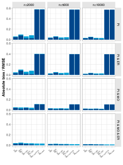
Figure 4: Estimators’ absolute bias and Root Mean Squared Error (RMSE) with parametric models including all the relevant variables, across twelve scenario/sample size combinations.

Absolute bias is the darker portion of each bar; RMSE corresponds to the total bar size. Abbreviations: PI = Principal Ignorability (Scenario 1), PI & ER = Principal Ignorability and Exclusion Restriction (Scenario 2), PI & MO= Principal Ignorability and Monotonicity (Scenario 3), PI & ER & MO = Principal Ignorability, Exclusion Restriction and Monotonicity (Scenario 4).

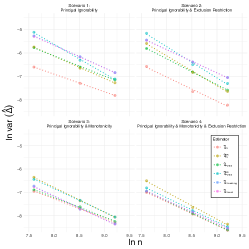
Figure 5: Estimators’ variance and rate of convergence with parametric models including all the relevant variables.

For each estimator/scenario combination, slopes describe rates of convergence (e.g., a slope of $-1/2$ points to a convergence speed of $\sqrt{n}$), while intercepts approximate the logarithm of asymptotic variances.

Table 2: Results of the simulation study where parametric models include all relevant variables.

Scenario	Scenario 1: Principal ignorability			Scenario 2: Principal ignorability, and exclusion restriction			Scenario 3: Principal ignorability, and monotonicity			Scenario 4: Principal ignorability, exclusion restriction, and monotonicity
	$\operatorname{\mathbb{E}}[Y^{t=1}-Y^{t=0}]=-2.13\%$	$\operatorname{\mathbb{E}}[(Y^{s=a,z=0,t=1}-Y^{s=a,z=1,t=1})^{2}]=60.74\%$	$\operatorname{\mathbb{E}}[\rho_{c}(X)]=55.08\%$	$\operatorname{\mathbb{E}}[Y^{t=1}-Y^{t=0}]=-5.79\%$	$\operatorname{\mathbb{E}}[(Y^{s=a,z=0,t=1}-Y^{s=a,z=1,t=1})^{2}]=0$	$\operatorname{\mathbb{E}}[\rho_{c}(X)]=55.08\%$	$\operatorname{\mathbb{E}}[Y^{t=1}-Y^{t=0}]=13.54\%$	$\operatorname{\mathbb{E}}[(Y^{s=a,z=0,t=1}-Y^{s=a,z=1,t=1})^{2}]=60.74\%$	$\operatorname{\mathbb{E}}[\rho_{c}(X)]=65.30\%$	$\operatorname{\mathbb{E}}[Y^{t=1}-Y^{t=0}]=10.08\%$	$\operatorname{\mathbb{E}}[(Y^{s=a,z=0,t=1}-Y^{s=a,z=1,t=1})^{2}]=0$	$\operatorname{\mathbb{E}}[\rho_{c}(X)]=65.30\%$
	$\Delta=20.31\%$	$\operatorname{\mathbb{E}}[(Y^{s=n,z=1,t=0}-Y^{s=a,z=0,t=0})^{2}]=54.90\%$	$\operatorname{\mathbb{E}}[\rho_{d}(X)]=14.36\%$	$\Delta=20.31\%$	$\operatorname{\mathbb{E}}[(Y^{s=n,z=1,t=0}-Y^{s=a,z=0,t=0})^{2}]=0$	$\operatorname{\mathbb{E}}[\rho_{d}(X)]=14.36\%$	$\Delta=20.31\%$	$\operatorname{\mathbb{E}}[(Y^{s=n,z=1,t=0}-Y^{s=a,z=0,t=0})^{2}]=54.90\%$	$\operatorname{\mathbb{E}}[\rho_{d}(X)]=0$	$\Delta=20.31\%$	$\operatorname{\mathbb{E}}[(Y^{s=n,z=1,t=0}-Y^{s=a,z=0,t=0})^{2}]=0$	$\operatorname{\mathbb{E}}[\rho_{d}(X)]=0$
Estimator	Bias	Empirical SE	RMSE	Bias	Empirical SE	RMSE	Bias	Empirical SE	RMSE	Bias	Empirical SE	RMSE
$n=2000$
$\widehat{\Delta}_{PI}$	-4.65%	3.68%	5.93%	-2.99%	3.73%	4.78%	-3.95%	3.09%	5.02%	-2.50%	3.02%	3.92%
$\widehat{\Delta}_{PI}^{ER}$	-7.85%	5.65%	9.67%	-7.95%	6.11%	10.03%	-2.39%	4.17%	4.81%	-3.05%	3.87%	4.93%
$\widehat{\Delta}_{PI,MO}$	-2.33%	5.59%	6.06%	-1.90%	5.48%	5.79%	-3.85%	3.18%	4.99%	-2.08%	3.09%	3.72%
$\widehat{\Delta}_{PI,MO}^{ER}$	-2.68%	7.76%	8.20%	-1.46%	7.58%	7.72%	-1.64%	3.99%	4.32%	-1.48%	3.32%	3.64%
$\widehat{\Delta}_{IV\,matching}$	57.57%	7.17%	58.01%	39.55%	6.56%	40.09%	10.78%	3.46%	11.32%	0.13%	3.10%	3.10%
$\widehat{\Delta}_{IV\,wald}$	57.52%	7.09%	57.96%	39.53%	6.53%	40.07%	10.76%	3.41%	11.29%	0.12%	3.08%	3.09%
$n=5000$
$\widehat{\Delta}_{PI}$	-2.92%	2.60%	3.91%	-1.59%	2.18%	2.69%	-2.52%	2.15%	3.32%	-1.52%	1.90%	2.43%
$\widehat{\Delta}_{PI}^{ER}$	-5.09%	3.59%	6.23%	-3.87%	3.28%	5.07%	-1.76%	2.53%	3.08%	-1.62%	2.19%	2.72%
$\widehat{\Delta}_{PI,MO}$	-1.61%	3.68%	4.01%	-1.01%	3.31%	3.46%	-2.38%	2.22%	3.25%	-1.23%	1.92%	2.28%
$\widehat{\Delta}_{PI,MO}^{ER}$	-1.22%	4.26%	4.43%	0.25%	3.88%	3.88%	-1.46%	2.55%	2.94%	-1.00%	2.04%	2.27%
$\widehat{\Delta}_{IV\,matching}$	57.29%	4.59%	57.47%	39.36%	4.11%	39.57%	10.64%	2.12%	10.84%	0.02%	1.98%	1.98%
$\widehat{\Delta}_{IV\,wald}$	57.28%	4.56%	57.46%	39.36%	4.08%	39.57%	10.64%	2.11%	10.85%	0.03%	1.97%	1.97%
$n=10000$
$\widehat{\Delta}_{PI}$	-2.40%	2.00%	3.13%	-1.24%	1.63%	2.05%	-2.19%	1.57%	2.69%	-1.34%	1.34%	1.90%
$\widehat{\Delta}_{PI}^{ER}$	-4.58%	2.63%	5.29%	-2.87%	2.18%	3.60%	-1.69%	1.78%	2.46%	-1.42%	1.53%	2.09%
$\widehat{\Delta}_{PI,MO}$	-1.69%	2.80%	3.27%	-1.07%	2.25%	2.49%	-2.10%	1.62%	2.65%	-1.11%	1.35%	1.75%
$\widehat{\Delta}_{PI,MO}^{ER}$	-0.90%	2.85%	2.99%	0.62%	2.59%	2.66%	-1.44%	1.78%	2.29%	-0.90%	1.45%	1.70%
$\widehat{\Delta}_{IV\,matching}$	57.21%	3.27%	57.31%	39.25%	2.94%	39.36%	10.58%	1.54%	10.70%	-0.02%	1.40%	1.40%
$\widehat{\Delta}_{IV\,wald}$	57.22%	3.26%	57.32%	39.26%	2.94%	39.37%	10.59%	1.53%	10.70%	-0.02%	1.40%	1.40%

References

- Angrist et al. (2000) Angrist, J. D., Graddy, K. and Imbens, G. W. (2000) The interpretation of instrumental variables estimators in simultaneous equations models with an application to the demand for fish. The Review of Economic Studies, 67, 499–527.
- Angrist et al. (1996) Angrist, J. D., Imbens, G. W. and Rubin, D. B. (1996) Identification of causal effects using instrumental variables. Journal of the American Statistical Association, 91, 444–455.
- Chernozhukov et al. (2018) Chernozhukov, V., Chetverikov, D., Demirer, M., Duflo, E., Hansen, C., Newey, W. and Robins, J. (2018) Double/debiased machine learning for treatment and structural parameters. The Econometrics Journal, 21, C1–C68.
- Chollet (2021) Chollet, F. (2021) Working with Keras: A deep dive, chap. 7, 172–200. Manning.
- Frangakis and Rubin (1999) Frangakis, C. E. and Rubin, D. B. (1999) Addressing complications of intention-to-treat analysis in the combined presence of all-or-none treatment-noncompliance and subsequent missing outcomes. Biometrika, 86, 365–379.
- Frangakis and Rubin (2002) — (2002) Principal stratification in causal inference. Biometrics, 58, 21–29.
- Frölich (2007) Frölich, M. (2007) Nonparametric IV estimation of local average treatment effects with covariates. Journal of Econometrics, 139, 35–75.
- Goetghebeur et al. (2020) Goetghebeur, E., le Cessie, S., De Stavola, B., Moodie, E. E., Waernbaum, I. and the topic group Causal Inference (TG7) of the STRATOS initiative (2020) Formulating causal questions and principled statistical answers. Statistics in medicine, 39, 4922–4948.
- Grolleau (2022) Grolleau, F. (2022) Mestim: Computes the Variance-Covariance Matrix of Multidimensional Parameters Using M-Estimation. URL: https://CRAN.R-project.org/package=Mestim. R package version 0.2.0.
- Heckman and Vytlacil (2001) Heckman, J. J. and Vytlacil, E. (2001) Policy-relevant treatment effects. American Economic Review, 91, 107–111.
- Hines et al. (2022) Hines, O., Dukes, O., Diaz-Ordaz, K. and Vansteelandt, S. (2022) Demystifying statistical learning based on efficient influence functions. The American Statistician, 76, 292–304.
- Imbens (2014) Imbens, G. (2014) Instrumental variables: an econometrician’s perspective. Tech. rep., National Bureau of Economic Research.
- Imbens and Angrist (1994) Imbens, G. W. and Angrist, J. D. (1994) Identification and estimation of local average treatment effects. Econometrica: Journal of the Econometric Society, 467–475.
- Imbens and Rubin (1997) Imbens, G. W. and Rubin, D. B. (1997) Bayesian inference for causal effects in randomized experiments with noncompliance. The Annals of Statistics, 305–327.
- International Council For Harmonisation of Technical Requirements For Pharmaceuticals For Human Use (2019) (ICH) International Council For Harmonisation of Technical Requirements For Pharmaceuticals For Human Use (ICH) (2019) E9(R1) Statistical Principles for Clinical Trials: Addendum: Estimands and Sensitivity Analysis in Clinical Trials.
- Jo and Stuart (2009) Jo, B. and Stuart, E. A. (2009) On the use of propensity scores in principal causal effect estimation. Statistics in Medicine, 28, 2857–2875.
- Jordan and Jacobs (1994) Jordan, M. I. and Jacobs, R. A. (1994) Hierarchical mixtures of experts and the EM algorithm. Neural Computation, 6, 181–214.
- Kramer et al. (2001) Kramer, M. S., Chalmers, B., Hodnett, E. D., Sevkovskaya, Z., Dzikovich, I., Shapiro, S., Collet, J.-P., Vanilovich, I., Mezen, I., Ducruet, T. et al. (2001) Promotion of breastfeeding intervention trial (PROBIT): a randomized trial in the republic of belarus. Jama, 285, 413–420.
- Kuo and Peng (2000) Kuo, L. and Peng, F. (2000) A mixture-model approach to the analysis of survival data. Generalized Linear Models: A Bayesian Perspective, 255.
- Little and Rubin (2000) Little, R. J. and Rubin, D. B. (2000) Causal effects in clinical and epidemiological studies via potential outcomes: concepts and analytical approaches. Annual Review of Public Health, 21, 121–145.
- Mansournia et al. (2017) Mansournia, M. A., Higgins, J. P., Sterne, J. A. and Hernán, M. A. (2017) Biases in randomized trials: a conversation between trialists and epidemiologists. Epidemiology, 28, 54.
- Prosperi et al. (2020) Prosperi, M., Guo, Y., Sperrin, M., Koopman, J. S., Min, J. S., He, X., Rich, S., Wang, M., Buchan, I. E. and Bian, J. (2020) Causal inference and counterfactual prediction in machine learning for actionable healthcare. Nature Machine Intelligence, 2, 369–375.
- Rosenbaum and Rubin (1983) Rosenbaum, P. R. and Rubin, D. B. (1983) The central role of the propensity score in observational studies for causal effects. Biometrika, 70, 41–55.
- Rubin (1978) Rubin, D. B. (1978) Bayesian inference for causal effects: The role of randomization. The Annals of statistics, 34–58.
- Saul and Hudgens (2020) Saul, B. C. and Hudgens, M. G. (2020) The calculus of M-estimation in R with geex. Journal of Statistical Software, 92, 1–15.
- Stefanski and Boos (2002) Stefanski, L. A. and Boos, D. D. (2002) The calculus of M-estimation. The American Statistician, 56, 29–38.
- Stuart and Jo (2015) Stuart, E. A. and Jo, B. (2015) Assessing the sensitivity of methods for estimating principal causal effects. Statistical Methods in Medical Research, 24, 657–674.
- Wald (1940) Wald, A. (1940) The fitting of straight lines if both variables are subject to error. The annals of mathematical statistics, 11, 284–300.
- Xu and Jordan (1993) Xu, L. and Jordan, M. I. (1993) EM learning on a generalized finite mixture for combining multiple classifiers. World Congress on Neural Networks, 4, 227–230.