Using finite automata to compute the base- representation of the golden ratio and other quadratic irrationals
Abstract
We show that the ’th digit of the base- representation of the golden ratio is a finite-state function of the Zeckendorf representation of , and hence can be computed by a finite automaton. Similar results can be proven for any quadratic irrational. We use a satisfiability (SAT) solver to prove, in some cases, that the automata we construct are minimal.
1 Introduction
The base- digits of famous irrational numbers have been of interest for hundreds of years. For example, William Shanks computed 707 decimal digits of in 1873 (but only the first 528 were correct) [18]. As a high school student, the third author used a computer in 1976 to determine the first digits of the decimal representation of , the golden ratio, using the computer language APL [15].
The celebrated results of Bailey, Borwein, and Plouffe [2] demonstrated that one can compute the ’th bit of certain famous constants, such as , in very small space.111Sometimes this result is described as “computing the ’th digit without having to compute the previous digits”. But this is not really a meaningful assertion, since the phrase “computing without computing ” is not so well-defined.
Can finite automata generate the base- digits of irrational algebraic numbers, such as ? This fundamental question was raised by Cobham in the late 1960’s (a re-interpretation of a related question due to Hartmanis and Stearns [9]). Though Cobham believed for a time that he had proved they cannot be so generated [7], his proof was flawed, and it was not until 2007 that Adamczewski and Bugeaud [1] succeeded in proving that there is no deterministic finite automaton with output that, on input expressed in base , returns the ’th base- digit of an irrational real algebraic number .
Even so, in this paper we show that, using finite automata, one can compute the ’th digit in the base- representation of the golden ratio ! At first glance this might seem to contradict the Adamczewski–Bugeaud result. But it does not, since for our theorem the input is not expressed in base , but rather in an entirely different numeration system, the Zeckendorf representation. Analogous results exist for any quadratic irrational.
Our result does not give a particularly efficient way to compute the base- digits of quadratic irrationals, but it is nevertheless somewhat surprising. Using a SAT solver, in some cases (such for the binary digits of ) we prove that the automata constructed is minimal and unique. Interestingly, in other cases (such as for the ternary digits of ) we were able to prove the minimality of our automaton, but we discovered several distinct automaton with the same number of states computing the same quadratic irrational (at least up to a very high precision). It is conceivable that the automata produced by our method are indeed minimal and unique in general, and we leave this as an open question.
2 Number representations and automata
A DFAO (deterministic finite automaton with output) consists of a finite number of states, and labeled transitions connecting them. The automaton processes an input string by starting in the distinguished start state , and then following the transitions from state to state, according to each successive bit of . Each state has an output associated with it, and the function computed by the DFAO maps the input to the output associated with the last state reached. For an example of a DFAO, see Figure 2.
A DFA (deterministic finite automaton) is quite similar to a DFAO. The only difference is that there are exactly two possible outputs associated with each state, either or . States with an output of are called “accepting” or “final”. If an input results in an output of , it is said to be accepted by the DFA. A synchronized DFA [6] is a particular type of DFA that takes two inputs in parallel; this is accomplished by making the input alphabet a set of pairs of alphabet symbols. A synchronized automaton computes a synchronized sequence ; it does this by accepting exactly the inputs where the first components spell out a representation of , and the second components spell out a representation for , where leading zeros may be required to make the inputs the same length. For more about synchronized sequences, see [16]. An example of a synchronized DFA appears in Figure 1.
Let be a non-negative real number, and write its base- representation in the form , where . For , we call the ’th digit to the right of the point. The indexing is perhaps a little unusual, but it seems to decrease the size of the automata produced.
2.1 Zeckendorf representation
The Fibonacci numbers are defined, as usual, by , , and . The Zeckendorf representation [11, 20] of a natural number is the unique way of writing as a sum of Fibonacci numbers , , subject to the condition that no two consecutive Fibonacci numbers are used. We may write the Zeckendorf representation as a binary string , where . For example, has representation . The substring cannot occur due to the rule that two consecutive Fibonacci numbers cannot be used. In what follows, leading zeros in strings are typically ignored without comment.
To illustrate these ideas, Table 1 gives the Zeckendorf representation of the first few powers of and . We will use them in Section 3.
| 0 | 1 | 1 | 1 | 1 |
| 1 | 2 | 10 | 3 | 100 |
| 2 | 4 | 101 | 9 | 10001 |
| 3 | 8 | 10000 | 27 | 1001001 |
| 4 | 16 | 100100 | 81 | 101001000 |
| 5 | 32 | 1010100 | 243 | 100000010010 |
3 Automata and the base- representation of
Our main result is Theorem 1 below.
Theorem 1.
For all integers , there exists a DFAO that, on input the Zeckendorf representation of , computes the ’th digit to the right of the point in the base- representation of .
Proof.
It is known that there exists a -state synchronized DFA accepting, in parallel, the Zeckendorf representations of and for all [17, Thm. 10.11.1(a)]. Its transition diagram is depicted in Figure 1, where accepting states are denoted by double circles, and is the initial state, labeled by a headless arrow entering.
The DFA is constructed using the fact that , where is the left shift of the string . For example, , and to determine , we find , left-shift that to get , and add to get .
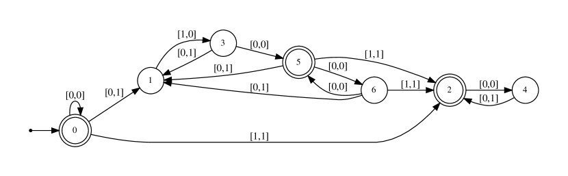
To understand how to use this automaton, observe that and and . Since these two numbers have representations of different lengths, we need to pad the former with a leading . Then if , the first components concatenated spell out and the second components spell out . When we input this, we visit, successively, states , and so we accept.
Let be a positive real number, with base- representation , where the period is the analogue of the decimal point for base , and is an arbitrary finite block of digits. Now has base- representation and has base- representation . Similarly, has base- representation . Hence . In the particular case where , we get a formula for the ’th digit to the right of the decimal point of , namely
From the DFA computing , it is possible to create another DFA accepting, in parallel, the Zeckendorf representations of and . This is based on the fact that there is an algorithm to compile a first-order logic statement involving the usual logical operations (AND, OR, NOT, etc.), the integer operations of addition, subtraction, multiplication by constants, and the universal and existential quantifiers, into an automaton that accepts the Zeckendorf representation of those integers making the statement true [12].
From this DFA, we can compute individual DFAs accepting the Zeckendorf representation of those for which , for . Finally, we combine all the together into a single DFAO (using a product construction for automata) computing the difference .
By substituting , we see that this automaton is the desired one, computing on input the Zeckendorf representation of . ∎
We now use Walnut, which is free software for compiling first-order logical expressions into automata, to explicitly compute the automata for in base and base . For base , we need the following Walnut commands:
reg shift {0,1} {0,1} "([0,0]|[0,1][1,1]*[1,0])*":
def phin "?msd_fib (s=0 & n=0) | Ex $shift(n-1,x) & s=x+1":
def phid2 "?msd_fib Ex,y $phin(2*n,x) & $phin(n,y) & x=2*y+1":
combine FD2 phid2:
These produce the DFAO in Figure 2.

For example, in base , we have . To compute the 4th digit to the right of the binary point we write in Zeckendorf representation, namely , and feed it into the automaton, reaching states successively, with output at the end.
We now explain the Walnut commands. The first line creates the DFA shift, using a regular expression; it takes two base- inputs and only accepts if the second input is the left shift of the first. Next is the DFA phin, which is shown in Figure 1 and uses shift to check that its two inputs have the relationship and , which computes the function in a synchronized fashion. Next, the DFA phid2, when given the representation of as input, accepts if , and rejects otherwise. Lastly, combine converts phid2 into a DFAO by replacing its accepting and rejecting states with output value and , respectively.
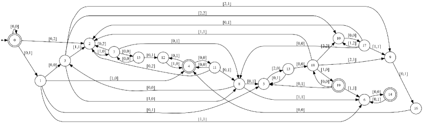
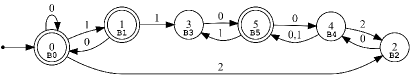
The automaton for base (see Figure 3) can be constructed similarly with the following Walnut commands:
reg shift {0,1} {0,1} "([0,0]|[0,1][1,1]*[1,0])*":
def phin "?msd_fib (s=0 & n=0) | Ex $shift(n-1,x) & s=x+1":
def phid3a "?msd_fib Ex,y $phin(3*n,x) & $phin(n,y) & x=3*y+1":
def phid3b "?msd_fib Ex,y $phin(3*n,x) & $phin(n,y) & x=3*y+2":
combine FD3 phid3a=1 phid3b=2:

In base , . To compute the rd digit to the right of the point we write in Zeckendorf representation as and pass it to the automaton, which traverses states successively, giving an output of .
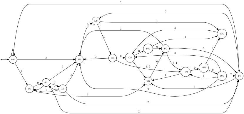
There is no conceptual barrier to carrying out similar computations for any base . For base , for example, Walnut computes a finite automaton with states that, on input , returns the ’th digit to the right of the decimal point in the decimal expansion of . The transition diagram is, unfortunately, too complicated to display here, but the transition table and output function is given in the Appendix.
4 Other quadratic irrationals
There is nothing special about , and the same ideas can be used for any quadratic irrational, although the input representation requires some modification.
4.1 Pell representation
Another representation for the natural numbers is based on the Pell numbers, defined by , , and for . We can then write every natural number where . To get uniqueness of the representation, we have to impose two conditions. First, we must have that . Second, if , then . See [4] for more details. The unique representation, over the alphabet , is denoted .
Table 2 gives the Pell representation of the first few powers of and . We will use them in Section 4.1.
| 0 | 1 | 1 | 1 | 1 |
| 1 | 2 | 10 | 3 | 11 |
| 2 | 4 | 20 | 9 | 120 |
| 3 | 8 | 111 | 27 | 2011 |
| 4 | 16 | 1020 | 81 | 100201 |
| 5 | 32 | 10011 | 243 | 1100020 |
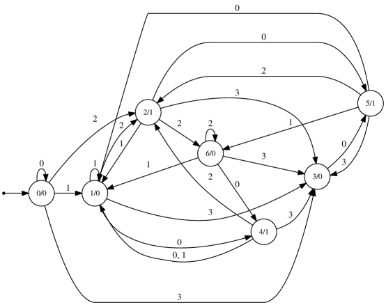
The Pell numeration system in Walnut can be used to construct automata computing the base- digits of , just as we did for . This results in a 6-state DFAO for base 2 (see Figure 4), and a 14-state DFAO for base 3. The Walnut commands for base 2 are:
reg pshift {0,1,2} {0,1,2}
   "([0,0]|([0,1][1,1]*([1,0]|[1,2][2,0]))|[0,2][2,0])*":
def sqrt2n "?msd_pell (s=0 & n=0) | Ex $pshift(n-1,x) & s=x+2":
def sqrt2d2 "?msd_pell Ex,y $sqrt2n(2*n,x) & $sqrt2n(n,y)
   & x=2*y+1":
combine SD2 sqrt2d2:

The alert reader will observe that no output is associated with state . This is because inputs that lead to this state, such as , are not valid Pell representations. However, the state cannot be removed, because is a valid Pell representation.
4.2 Ostrowski representation
Of course, what makes our results work is that the numeration systems are “tuned” to the particular quadratic irrational we want to compute. For , this is the Fibonacci numbers; for , the Pell numbers. We need to find an appropriate numeration system that is similarly “tuned” to any quadratic irrational. It turns out that the proper system is the Ostrowski numeration system [3, 13].
Every irrational real number can be expressed uniquely as an infinite simple continued fraction . Furthermore, is called the denominator of a convergent for if , , and for . For example, the continued fraction for is , corresponding to the sequence .
The Ostrowski -numeration system uses the sequence of the denominators of the convergents for to construct a unique representation for a non-negative integer expressed as
where
-
1.
;
-
2.
for ; and
-
3.
for , if then .
The Ostrowski -representation for is then determined with a greedy algorithm, starting at the most significant term and choosing the largest multiple for that is less than , and then applying the same algorithm to . For example, for , the denominators of the continued fraction convergents form the sequence (OEIS A002530). Rule for the construction forces because , while rule requires that , and so on. Rule ensures uniqueness by enforcing the constraint that if , then , and if , then , and so on. Then, for example, the -representation of .
In order to construct a DFAO that, given the input of the Ostrowski -representation of , computes the ’th digit to the right of the point in the base- representation of , we require an Ostrowski -synchronized function . It was shown in [14] that every quadratic irrational with a purely periodic continued fraction has an Ostrowski -synchronized sequence , such that
| (1) |
where is the denominator of the ’th convergent to , and is the -representation of , left-shifted times.
Furthermore, it was shown that if belongs to , then is synchronized in terms of the Ostrowski -representation through the relation , where , , and
| (2) |
This is notable because when constructing an Ostrowski -representation with Walnut, it is assumed that , which corresponds to a continued fraction with terms and . If , then we can set and rotate the period until , giving a quadratic irrational corresponding to the periodic part of . Then an Ostrowski representation for can be constructed, and Eq. (1) is used to find an automaton for , followed by Eq. (2) to find an automaton for . Therefore, is synchronized in terms of the Ostrowski -representation.
For example, for , we have . Since we only compute the digits after the decimal point, we set and then rotate the period to get . This gives the sequence of denominator convergents , where , , and , and so Eq. (1) gives . This results in a DFA for that has 23 states. Then, we find , with , , and , and Eq. (2) gives a DFA with 20 states, shown in Figure 5.
Then, for example and and . When we input into the automaton, we visit states in succession, and so we accept. From here, the same process that is outlined in Section 3 can be used to construct a DFA accepting in parallel the Ostrowski -representations of and , and ultimately the DFAO as desired.
4.3 Walnut implementation
Constructing the DFAOs for other quadratic irrationals with Walnut requires the ost command to create custom Ostrowski representations. As explained above, Walnut requires that to create the corresponding Ostrowski representation, and it is possible to create a DFAO for by synchronizing it in terms of the the Ostrowski representation for . Presented below are the general steps for constructing a DFAO for a quadratic irrational with Walnut, using the process explained above with Equations (1) and (2).
First, we construct the continued fraction of from by setting and rotating the period until , if necessary. Next, we determine the denominators and of the continued fraction convergent to , where is the number of elements in the period. Lastly, we find , , and from the relation , where . With these, we can use the following Walnut commands:
# Construct Ostrowski representation for Beta
    ost ostBeta [0] [d1 d2 ... dm];
# Create a DFA of z = floor(n*Beta) using j and k
    def betan "?msd_ostBeta Eu,v n=u+1 & $shift(u,v) & v=k*z+j*u":
# Create a DFA of z = floor(n*Alpha) synchronized
    def alphan "?msd_ostBeta Eu $betan(b*n,u) & z=(u+a*n)/c":
# Create a DFAO for Alpha in base 2
    def alphan_d2 "?msd_ostBeta Ex,y $alphan(2*n,x) & $alphan(n,y)
    & x!=2*y":
    combine AD2 alphan_d2:
The shift DFA can be constructed from a regular expression as done above for , and is based on the specific representation and continued fraction sequence. If multiple left-shifts are required, it may be simpler to create a shift DFA that left-shifts only one position at a time, and chain its use together multiple times. For example, three left-shifts could be achieved using a 1-shift DFA by:
def betan "?msd_ostBeta Eu,v,w,x n=u+1 & $shift(u,v) & $shift(v,w)
       & $shift(w,x) & x=k*z+j*u":
Using this process, we created the DFAOs for other quadratic irrationals including the “bronze ratio” and several Pisot numbers.
4.4 Walnut code for quadratic irrationals
In this section we give Walnut code and provide the resulting automata for several more quadratic irrationals, including the “bronze ratio” in bases 2 and 3. We also provide code that construct automata computing the Pisot numbers and and some other closely related quadratic irrationals.
4.4.1 The bronze ratio in base and base
ost bt [0] [3];
reg bts {0,1,2,3} {0,1,2,3}
   "([0,0]|[0,2][2,2]*[2,0]|([0,2][2,2]*[2,3]|[0,3])
   [3,0]|([0,1]|[0,2][2,2]*[2,1])([1,1]|[1,2][2,2]*[2,1])*
   (([1,2][2,2]*[2,3]|[1,3])[3,0]|[1,2][2,2]*[2,0]|[1,0]))*":
def btbn "?msd_bt Eu,v n=u+1 & $bts(u,v) & v=1*z+3*u":
def btan "?msd_bt Eu $btbn(1*n,u) & z=(u+3*n)/1":
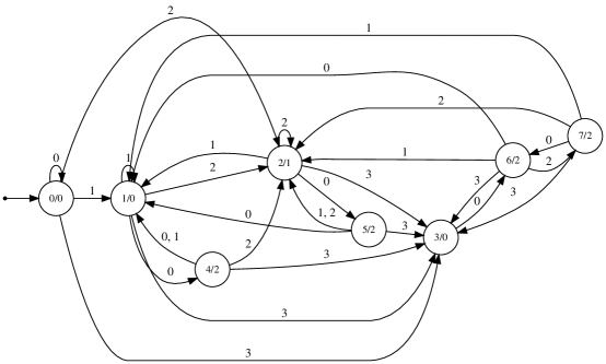
DFAO for the bronze ratio in base 2 (see Figure 6):
def btn_d2 "?msd_bt Ex,y $btan(2*n,x) & $btan(n,y) & x!=2*y":
combine BTND2 btn_d2:
DFAO for the bronze ratio in base 3 (see Figure 7):
def btn_d3a "?msd_bt Ex,y $btan(3*n,x) & $btan(n,y) & x=3*y+1":
def btn_d3b "?msd_bt Ex,y $btan(3*n,x) & $btan(n,y) & x=3*y+2":
combine BTND3 btn_d3a btn_d3b:
4.4.2 Pisot number and in base
ost pv1 [0] [2 1];
reg pv1s {0,1,2} {0,1,2} "([0,0]|([0,1][1,1][1,0]|[0,1][1,0])|
     [0,2][2,0])*":
def pv1bn "?msd_pv1 Et,u,v n=t+1 & $pv1s(t,u) & $pv1s(u,v)
   & v=2*z+3*t":
DFAO for in base 2:
def pv1bn_d2 "?msd_pv1 Ex,y $pv1bn(2*n,x) & $pv1bn(n,y) & x!=2*y":
combine PV1B2 pv1bn_d2:
DFAO for in base 2:
def pv1an "?msd_pv1 Eu $pv1bn(2*n,u) & z=(u+2*n)/1":
def pv1n_d2 "?msd_pv1 Ex,y $pv1an(2*n,x) & $pv1an(n,y) & x!=2*y":
combine PV12 pv1n_d2:
4.4.3 Pisot number and in base
ost pv2 [0] [3 1 1];
reg pv2s {0,1,2,3} {0,1,2,3}
   "([0,0]|[0,1][1,0]|[0,1][1,1][1,0]|[0,2][2,0]|
   [0,2][2,1][1,0]|[0,3][3,0])*":
def pv2bn "?msd_pv2 Es,t,u,v n=s+1 & $pv2s(s,t)
   & $pv2s(t,u) & $pv2s(u,v) & v=4*z+7*s":
DFAO for in base 2 (see Figure 8):
def pv2bn_d2 "?msd_pv2 Ex,y $pv2bn(2*n,x) & $pv2bn(n,y) & x!=2*y":
combine PV2B2 pv2bn_d2:
DFAO for in base 2:
def pv2an "?msd_pv2 Eu $pv2bn(2*n,u) & z=(u+3*n)/1":
def pv2n_d2 "?msd_pv2 Ex,y $pv2an(2*n,x) & $pv2an(n,y) & x!=2*y":
combine PV22 pv2n_d2:
5 Are the automata minimal?
The automata that Walnut constructs for computing on input are guaranteed to be minimal. However, in this paper, with our application to computing the base- digits of , we are only interested in running these automata in the special case when , the powers of . Could it be that there are even smaller automata that answer correctly on inputs of the form (but might give a different answer for other inputs)? After all, for each , we are only concerned with behavior of the automaton on linearly many inputs of length , as opposed to the exponentially large set of valid length- Zeckendorf representations. Thus, the automaton is not very constrained.
We do not know the answer to this question, in general. The question is likely difficult; in terms of computational complexity, it is a special case of a problem known to be NP-hard, namely, the problem of inferring a minimal DFAO from incomplete data [8]. However, this problem can sometimes be solved in practice using satisfiability (SAT) solving [19].
We are able to show that some of our automata are indeed minimal, among all automata giving the correct answers on inputs of the form , and satisfying two conventions: first, that leading zeroes in the input cannot affect the result, and second, that the automata obey the Ostrowski rules for the particular numeration system. Our method of proving minimality (and in some cases uniqueness) uses SAT solving.
We use a modified version of a MinDFA solver called DFA-Inductor [19] to generate SAT encodings for minimal automata, which are then passed to the CaDiCaL SAT solver [5] to determine whether they have a satisfying solution. DFA-Inductor uses the compact encoding method given by Heule and Verwer [10], which defines eight constraints—four mandatory and four redundant—to translate DFA identification into a graph coloring problem, and then encodes those constraints into a SAT instance. In short, a set of accepting and rejecting strings from a given dictionary are used to construct an automaton called an augmented prefix tree acceptor (APTA), which is then used to construct a consistency graph (CG) made up from vertices of the APTA. Edges in the consistency graph identify the vertices of the APTA that cannot be safely merged together, and by partitioning the vertices as disjoint sets of equivalent states and iterating over the number of partitions, a minimal DFA can be constructed. Symmetry-breaking predicates are used to enforce a lexicographic breadth-first search (BFS) enumeration on the ordering of states in the constructed DFA, which reduces the size of the search space by removing isomorphic automata from consideration [19].
One of the redundant constraints of the compact encoding method adds all of the determinization conflicts from the consistency graph as binary clauses in the encoding. We found it was often the case that the time required to run the determinization step during the generation of the consistency graph was considerably higher than the time required by the solver to find a solution without the extra clauses. Therefore, we excluded the determinization step, so that only direct conflicts between accepting and rejecting states were added as binary clauses.
DFA-Inductor only supports DFAs (and hence only accepting or rejecting states), however, and additional output status labels were added for bases larger than 2. DFA-Inductor does not explicitly encode a “dead state” rejecting invalid strings, but a transition to a dead state can be implied by a lack of an outgoing transition on a given state. Another redundant constraint of the compact encoding method forces each state to have an outgoing transition on every symbol, which is required under the formal definition of a DFA. In order to accommodate the virtual dead state requirement, the constraint must be amended to exclude whichever symbols must transition to the implied dead state.
Our automata follow the convention that the start state consumes leading ’s in the input string. In terms of the compact encoding variables, indicates that state has a transition to state on label , or in the context of graph coloring, that parents of vertices with color and incoming label must have color . This constraint is then implemented by enforcing state to have a self-loop on the symbol using the unit clause , and the dictionary given to DFA-Inductor states that the string produces output .
In order for the SAT solver to construct automata that obey the rules of a given Ostrowski representation, we encode the Ostrowski rules as a set of constraints. Without these constraints, the solver may find a smaller DFAO by allowing rule-breaking transitions—such as allowing consecutive 1’s for in the Zeckendorf representation. In Section 5.1, we provide a SAT encoding of the Ostrowski rules for quadratic irrationals with a purely periodic continued fraction with a period of 1, such as , , and . In Section 5.2, we provide an encoding for purely periodic quadratic irrationals with longer periods, like and .
5.1 A simple Ostrowski encoding for metallic means
A metallic mean is a quadratic irrational with only a single repeating term in its period. When considering how to encode the three rules for the Ostrowski -representation of , we can think of each transition in the DFA as choosing a value for , starting with and working down to . Rule 1 requires that , which is enforced by requiring all strings in the dictionary to be valid strings in the representation, rather than through constraints on the solver. In the context of the metallic means, rule 2 requires that for all , which equates to restricting the set of valid transition labels for each state to be in the range of to . This is done automatically during the construction of the APTA, because is the largest value in the dictionary and thus the highest possible transition label. For , rule 3 requires that if , then ; this is the only constraint that must be explicitly encoded. Since every state has the same set of allowed transitions, we only need to enforce that no state have a self-loop on label , and that if state transitions to on label , then must transition to the dead state on labels to . Since dead states are implicit, the constraint is implemented by removing all outgoing transitions from except . The constraints are
where is the set of states in the resulting DFAO.
5.2 Ostrowski encoding for purely periodic quadratic irrationals
Quadratic irrationals of the form , where , require a more robust encoding than the metallic means in order to account for multiple terms in the period. The order of terms in the continued fraction determines the set of valid transitions between any two states. Therefore, the SAT solver must understand how to relate a given state in the DFAO to a given term in the continued fraction, otherwise the resulting DFAO may fail to reject invalid strings. We now present one such encoding.
Each Ostrowski -representation is a language made up from the set of valid strings that can be constructed using the Ostrowski rules. This language is recognized by a canonical DFA, and serves as the base that informs the valid structure of the final DFAO. Constructing a DFAO using only the states in the base DFA guarantees that rule 2 and rule 3 of the Ostrowski construction are never violated. Furthermore, a minimal complete DFAO constructed from only the base states is guaranteed to be minimal for the language. If it were possible to construct an even smaller complete DFAO that is still correct, then a state would exist that is not in the base DFA, implying that at least two unique base states could be safely combined, and thus that the canonical base DFA is not minimal. Therefore, the base states describe the complete set of rules the SAT solver must understand in order to construct a valid DFAO. Conveniently, Walnut automatically generates a DFA of the Ostrowski base during the process of constructing the representation.
Since each state in the base DFA has a unique transition set, we can refer to the ’th state in the base DFA as the ’th base state. For example, Figure 9 shows for how each base state in the Ostrowski base DFA (bottom), labelled B0 to B5, correspond exactly to a state in the DFAO for returning the ’th digit of in base 2 (top).
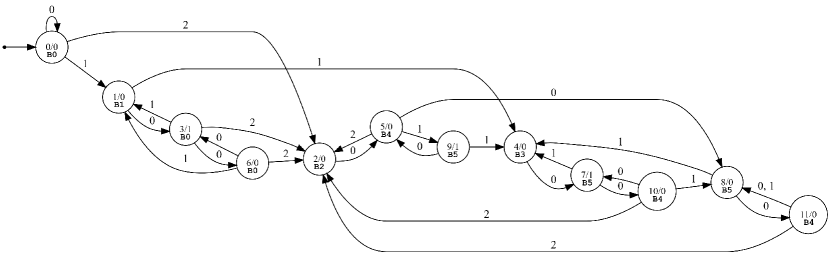
Each cyclic permutation of terms in the continued fraction requires a unique SAT encoding for the states of the Ostrowski base DFA. Term orderings that preserve the permutation differ only in which base states are accepting or rejecting. Since the dictionary file contains only accepted strings, the SAT solver does not need to know from this encoding which states of the Ostrowski base DFA should be rejecting, and so only the transition set of each base type is encoded.
The Ostrowski rules are encoded through the states in the Ostrowski base DFA by constraining each state in the DFAO to match a certain base state. Therefore, to encode the base states, we create a new variable , which says state in the DFAO is related to base state in the Ostrowski base DFA. We then relate the variable to the transition variable , which constrains the set of valid transitions between and according to which base states they are associated with. The encoding is presented in Table 3.
The last constraint in the table is the only one that needs to be manually determined for each Ostrowski base DFA, depending on the permutation of term orderings in the continued fraction. For example, for in Figure 9, base state B4 is encoded as follows, where denotes the set of states in the DFAO and denotes the set of states in the Ostrowski base DFA:
| Constraints | Range | Meaning |
|---|---|---|
| The start state can only have a self-loop on 0. | ||
| No states other than the start state can have a self-loop on any label. | ||
| The start state is related to base state 0. | ||
| ; | Each state in the DFAO must be related to at most one base type. | |
| Each state in the DFAO must be related to at least one base type. | ||
| ; ; ; | Suppose DFAO state is related to base state , and state is related to base state . If state in the base DFA does not have a transition to state on label , then cannot have a transition to on label in the DFAO. |
5.3 Results
Table 4 gives our results of DFA minimization by SAT on a few quadratic irrationals. In each of the cases, the Walnut solution was confirmed to be minimal by proving that there are no satisfying assignments of the SAT encoding with a smaller number of states than in the Walnut-produced automaton.
The dictionary containing the Ostrowski representation of the first digits is referred to as the ’th digit set. The solver is run on the SAT encoding of each digit set for a given number of states. The state count was increased every time the solver returned UNSAT, and the digit set was increased every time a satisfying assignment was found. Once the state count given by the Walnut-produced solution was reached, the solver was run exhaustively to find all satisfying assignments of the SAT formula and therefore all candidates for the minimal automata computing the quadratic irrational. However, most satisfying assignments encoded automata that only computed the given digit set correctly and did not correctly compute the digits of the quadratic irrational at high precision.
| Quadratic Irrational | base 2 8 states | base 3 13 states | base 2 6 states | base 2 7 states | base 3 8 states | base 2 12 states | base 2 16 states |
|---|---|---|---|---|---|---|---|
| Digit set size | 54 | 197 | 29 | 64 | 64 | 27 | 57 |
| SAT time (sec) | 0.50 | 28,425.5 | 0.08 | 142.81 | 44.68 | 0.14 | 68.11 |
| UNSAT time (sec) | 0.18 | 12,123.0 | 0.02 | 0.52 | 24.76 | 0.08 | 2.59 |
| Number of candidates | 1 | 3 | 1 | 3 | 7 | 1 | 9 |
The digit set size given in Table 4 is the smallest dictionary required for the SAT solver to find the -state Walnut solution. The SAT time is the time required by the solver to find the Walnut automaton. The UNSAT time is the time required determine no automata is possible using states. Since no candidate solutions are found at states, we conclude that the -state Walnut solution is minimal.
In some cases, multiple distinct candidates were found that correctly computed at least 10,000 digits of the quadratic irrational (see the last row of Table 4). For reference, the Walnut solutions for the cases with multiple candidate solutions are given in Section 4.4. For all except , these candidate solutions differ from the Walnut solution only by their outgoing transitions on the start state. The candidates for (base 3) and (base 2) have differing transitions on label 1, while the candidates for (base 3) differ on label 2. All of the candidates for have the same start state, but differ in their transitions on label 2. Given how similar the candidate solutions are to the Walnut solution and that they are correct up to a high precision, it is possible that the Walnut solution is not unique, though we leave this as an open problem.
Minimization of DFAOs for this purpose presents a particular challenge for the SAT solver, as both the size of the digit set required to find a candidate solution and the length of the representation for each digit position can be arbitrarily large. For this reason, in base 4 and in base 3 encountered prohibitively long solving times before the required number of states (22 states and 14 states, respectively) could be reached, preventing the minimality of the Walnut solutions from being determined. For in base 4, it took over 25 hours for the 78’th digit set to be declared UNSAT at 13 states, and for in base 3, it took over 55 hours for the 258’th digit set to be declared SAT at 11 states, but the satisfying assignment found by the solver corresponded to an automata that incorrectly computed the ternary digits of starting at the 321’th digit.
References
- [1] B. Adamczewski and Y. Bugeaud. On the complexity of algebraic numbers I. Expansions in integer bases. Ann. Math. 165 (2007), 547–565.
- [2] D. Bailey, P. Borwein, and S. Plouffe. On the rapid computation of various polylogarithmic constants. Math. Comp. 66 (1997), 903–913.
- [3] A. R. Baranwal, L. Schaeffer, and J. Shallit. Ostrowski-automatic sequences: theory and applications. Theoret. Comput. Sci. 858 (2021), 122–142.
- [4] A. R. Baranwal and J. Shallit. Critical exponent of infinite balanced words via the Pell number system. In R. Mercaş and D. Reidenbach, editors, WORDS 2019, Vol. 11682 of Lecture Notes in Computer Science, pp. 80–92. Springer-Verlag, 2019.
- [5] Armin Biere, Katalin Fazekas, Mathias Fleury, and Maximillian Heisinger. CaDiCaL, Kissat, Paracooba, Plingeling and Treengeling entering the SAT Competition 2020. In Tomas Balyo, Nils Froleyks, Marijn Heule, Markus Iser, Matti Järvisalo, and Martin Suda, editors, Proc. of SAT Competition 2020 – Solver and Benchmark Descriptions, Vol. B-2020-1 of Department of Computer Science Report Series B, pp. 51–53. University of Helsinki, 2020.
- [6] A. Carpi and C. Maggi. On synchronized sequences and their separators. RAIRO Inform. Théor. App. 35 (2001), 513–524.
- [7] A. Cobham. On the Hartmanis-Stearns problem for a class of tag machines. In IEEE Conference Record of 1968 Ninth Annual Symposium on Switching and Automata Theory, pp. 51–60, 1968. Also appeared as IBM Research Technical Report RC-2178, August 23 1968.
- [8] M. E. Gold. Complexity of automaton identification from given data. Inform. Control 37 (1978), 302–320.
- [9] J. Hartmanis and R. E. Stearns. On the computational complexity of algorithms. Trans. Amer. Math. Soc. 117 (1965), 285–306.
- [10] M. Heule and S. Verwer. Exact DFA identification using SAT solvers. In J. M. Sempere and P. García, editors, ICGI 2010, Vol. 6339 of Lecture Notes in Artificial Intelligence, pp. 66–79. Springer-Verlag, 2010.
- [11] C. G. Lekkerkerker. Voorstelling van natuurlijke getallen door een som van getallen van Fibonacci. Simon Stevin 29 (1952), 190–195.
- [12] H. Mousavi, L. Schaeffer, and J. Shallit. Decision algorithms for Fibonacci-automatic words, I: Basic results. RAIRO Inform. Théor. App. 50 (2016), 39–66.
- [13] A. Ostrowski. Bemerkungen zur Theorie der Diophantischen Approximationen. Abh. Math. Sem. Hamburg 1 (1922), 77–98, 250–251. Reprinted in Collected Mathematical Papers, Vol. 3, pp. 57–80.
- [14] L. Schaeffer, J. Shallit, and S. Zorcic. Beatty sequences for a quadratic irrational: decidability and applications. Arxiv preprint arXiv:2402.08331 [math.NT]. Available at https://arxiv.org/abs/2402.08331, 2024.
- [15] Jeffrey Shallit. Calculation of and (the golden ratio) to 10,000 decimal places. Reviewed in Math. Comp. 30 (1976), 377, 1976.
- [16] J. Shallit. Synchronized sequences. In T. Lecroq and S. Puzynina, editors, WORDS 2021, Vol. 12847 of Lecture Notes in Computer Science, pp. 1–19. Springer-Verlag, 2021.
- [17] J. Shallit. The Logical Approach To Automatic Sequences: Exploring Combinatorics on Words with Walnut, Vol. 482 of London Math. Society Lecture Note Series. Cambridge University Press, 2023.
- [18] W. Shanks. On the extension of the numerical value of . Proc. Roy. Soc. London 21 (1873), 318–319.
- [19] I. Zakirzyanov, A. Shalyto, and V. Ulyantsev. Finding all minimum-size DFA consistent with given examples: SAT-based approach. In A. Cerone and M. Roveri, editors, Software Engineering and Formal Methods: SEFM 2017 Collocated Workshops, Vol. 10729 of Lecture Notes in Computer Science, pp. 117–131. Springer-Verlag, 2018.
- [20] E. Zeckendorf. Représentation des nombres naturels par une somme de nombres de Fibonacci ou de nombres de Lucas. Bull. Soc. Roy. Liège 41 (1972), 179–182.
Appendix A Appendix
In this Appendix we give an automaton that computes the digits of in base 10. This DFAO has transition function and output function , with initial state and state set . The transition function and output are given in Table 5.
This was generated with the following Walnut code:
reg shift {0,1} {0,1} "([0,0]|[0,1][1,1]*[1,0])*":
def phin "?msd_fib (s=0 & n=0) | Ex $shift(n-1,x) & s=x+1":
def fibdigit "?msd_fib Ex,y $phin(10*n,x) & $phin(n,y) & z+10*y=x":

def fibd1 "?msd_fib $fibdigit(n,1)":
def fibd2 "?msd_fib $fibdigit(n,2)":
def fibd3 "?msd_fib $fibdigit(n,3)":
def fibd4 "?msd_fib $fibdigit(n,4)":
def fibd5 "?msd_fib $fibdigit(n,5)":
def fibd6 "?msd_fib $fibdigit(n,6)":
def fibd7 "?msd_fib $fibdigit(n,7)":
def fibd8 "?msd_fib $fibdigit(n,8)":
def fibd9 "?msd_fib $fibdigit(n,9)":

combine FD10 fibd1 fibd2 fibd3 fibd4 fibd5 fibd6 fibd7 fibd8 fibd9:

# FD10[10^n] gives the n’th digit in the decimal
# representation of phi = 1.61803...
| 0 | 0 | 1 | 0 | 49 | 46 | 27 | 9 |
| 1 | 2 | — | 6 | 50 | 71 | — | 5 |
| 2 | 3 | 4 | 2 | 51 | 72 | 30 | 1 |
| 3 | 5 | 6 | 8 | 52 | 73 | — | 7 |
| 4 | 7 | — | 4 | 53 | 32 | 74 | 3 |
| 5 | 8 | 9 | 0 | 54 | 75 | 1 | 9 |
| 6 | 10 | — | 7 | 55 | 35 | — | 6 |
| 7 | 11 | 12 | 3 | 56 | 76 | 6 | 8 |
| 8 | 13 | 14 | 9 | 57 | 77 | — | 7 |
| 9 | 15 | — | 5 | 58 | 78 | 12 | 3 |
| 10 | 16 | 17 | 1 | 59 | 79 | 47 | 9 |
| 11 | 18 | 19 | 7 | 60 | 80 | 17 | 1 |
| 12 | 20 | — | 4 | 61 | 51 | 19 | 7 |
| 13 | 21 | 22 | 0 | 62 | 81 | 55 | 0 |
| 14 | 23 | — | 6 | 63 | 24 | 4 | 2 |
| 15 | 24 | 25 | 2 | 64 | 26 | 82 | 8 |
| 16 | 26 | 27 | 8 | 65 | 83 | — | 4 |
| 17 | 28 | — | 5 | 66 | 29 | 9 | 1 |
| 18 | 29 | 30 | 1 | 67 | 84 | — | 7 |
| 19 | 31 | — | 7 | 68 | 61 | 85 | 3 |
| 20 | 32 | 33 | 3 | 69 | 86 | — | 5 |
| 21 | 34 | 14 | 9 | 70 | 87 | 37 | 2 |
| 22 | 35 | — | 5 | 71 | 88 | 45 | 2 |
| 23 | 36 | 37 | 2 | 72 | 46 | 89 | 9 |
| 24 | 38 | 39 | 8 | 73 | 72 | 50 | 1 |
| 25 | 40 | 0 | 4 | 74 | 90 | — | 3 |
| 26 | 41 | 42 | 0 | 75 | 54 | 1 | 0 |
| 27 | 43 | — | 6 | 76 | 91 | 9 | 0 |
| 28 | 44 | 45 | 3 | 77 | 16 | 92 | 1 |
| 29 | 46 | 47 | 9 | 78 | 18 | 19 | 8 |
| 30 | 48 | — | 5 | 79 | 41 | 22 | 0 |
| 31 | 49 | 50 | 1 | 80 | 46 | 27 | 8 |
| 32 | 51 | 52 | 7 | 81 | 34 | 1 | 9 |
| 33 | 53 | — | 3 | 82 | 77 | — | 6 |
| 34 | 54 | 55 | 0 | 83 | 44 | 12 | 3 |
| 35 | 56 | 4 | 2 | 84 | 80 | 50 | 1 |
| 36 | 5 | 57 | 8 | 85 | 53 | — | 4 |
| 37 | 58 | — | 4 | 86 | 93 | 4 | 2 |
| 38 | 59 | 9 | 1 | 87 | 94 | 82 | 8 |
| 39 | 60 | — | 7 | 88 | 38 | 67 | 8 |
| 40 | 61 | 12 | 3 | 89 | 95 | — | 6 |
| 41 | 62 | 14 | 9 | 90 | 96 | 74 | 3 |
| 42 | 63 | — | 5 | 91 | 13 | 47 | 9 |
| 43 | 64 | 65 | 1 | 92 | 83 | — | 5 |
| 44 | 66 | 67 | 8 | 93 | 76 | 39 | 8 |
| 45 | 68 | — | 4 | 94 | 8 | 42 | 0 |
| 46 | 41 | 69 | 0 | 95 | 87 | 65 | 2 |
| 47 | 70 | — | 6 | 96 | 73 | 52 | 7 |
| 48 | 24 | 25 | 2 |