A Mathematical Model of the Hidden Feedback Loop Effect in Machine Learning Systems
Abstract
Widespread deployment of societal-scale machine learning systems necessitates a thorough understanding of the resulting long-term effects these systems have on their environment, including loss of trustworthiness, bias amplification, and violation of AI safety requirements. We introduce a repeated learning process to jointly describe several phenomena attributed to unintended hidden feedback loops, such as error amplification, induced concept drift, echo chambers and others. The process comprises the entire cycle of obtaining the data, training the predictive model, and delivering predictions to end-users within a single mathematical model. A distinctive feature of such repeated learning setting is that the state of the environment becomes causally dependent on the learner itself over time, thus violating the usual assumptions about the data distribution. We present a novel dynamical systems model of the repeated learning process and prove the limiting set of probability distributions for positive and negative feedback loop modes of the system operation. We conduct a series of computational experiments using an exemplary supervised learning problem on two synthetic data sets. The results of the experiments correspond to the theoretical predictions derived from the dynamical model. Our results demonstrate the feasibility of the proposed approach for studying the repeated learning processes in machine learning systems and open a range of opportunities for further research in the area.
Keywords machine learning repeated learning hidden feedback loop dynamical systems concept drift
1 Introduction
Societal-scale machine learning and decision making systems are, by definition, intended to have a major impact on society as a whole. Recent analysis (CAIS, 2023) presents a wide range of potential problems and areas of concern associated with such systems (Suresh et al., 2020). Addressing these challenges and various aspects of engineering trustworthy systems (Li et al., 2023) requires different methods for designing machine learning and artificial intelligence systems, combining formal mathematical modelling, data-driven engineering methods, long-term risk analysis (Sifakis and Harel, 2023; Pei et al., 2022; He et al., 2021). One of the key quality attributes of trustworthy ML systems (Serban et al., 2021; Toreini et al., 2020; Siebert et al., 2020) and socially responsible AI (SRA) algorithms (Cheng et al., 2021) systems is their ability to behave in a way that users expect without any unintended side-effects.
A repeated machine learning process describes a situation in a machine learning system where the input data to a learning algorithm may depend in part on the previous predictions made by the system.
Machine learning methods usually take specific assumptions about the data, such as data has to be i.i.d., or stationary with white noise, or the environment the agent operates in remains the same, or there is a data drift independent from the learning agent. A distinctive feature of the repeated learning setting—the one that justifies introducing the name—is that the state of the environment in the process becomes causally dependent on the learning algorithm and the predictions given.
When there is a high automation bias, that is, when the use of predictions is high and adherence to them is tight, a so-called positive feedback loop occurs (Khritankov, 2021). As a result of the loop, the learning algorithm is repeatedly applied to the data containing previous predictions. This repeated learning produces a noticeable unintended shift in the distributions of the input data and the predictions of the system (Khritankov, 2023). Therefore, such a machine learning system would violate the trustworthiness requirements for socially responsible AI algorithms.
In many cases, the repeated ML process can represent the behaviour of a system interacting with its users. For example, in systems that recommend products to consumers or forecast market prices (Khritankov and Pilkevich, 2021; Sinha et al., 2016) and learn from user responses, healthcare decision support systems (Adam et al., 2020), and predictive policing and public safety systems (Ensign et al., 2018) that introduce bias in the training data as a result of an unintended feedback loop.
The main contribution of this paper is a dynamical systems (Galor, 2007) model of the repeated machine learning process. Formally, we consider a set F of probability density functions (PDFs), each of which describes the data available to a machine learning system at a given time step . We then introduce a mapping that acts on a given density function to produce a new data distribution . A general model of the repeated learning process we are studying can be written as
In this model, the mapping may include the following actions performed by the system: sampling training data from , learning or updating parameters of a predictive model, taking inputs and providing one or more predictions to users. The application of the mapping results in a new probability distribution with a density function .
The structure of the paper is as follows. In Section 2 we provide background on the problem of the hidden feedback loops and related work. In Section 3, we formally describe the mathematical model of the repeated learning process and reframe the aforementioned trustworthiness problems as research questions in terms of dynamical systems models. We then present our main theoretical results in Section 4. We find sufficient conditions for mapping to be a transformation on F. We find the limiting set and autonomy criterion for the dynamical system we introduce, prove convergence conditions and sufficient conditions for the mapping to be a non-contraction. In Section 5 we test our theoretical results in a series of experiments on several data sets.
2 Related Work
Let us give some background to the problem we are investigating. In many practical applications, the context in which a machine learning system is used may itself change the training data over time. Such data drift may be due to some external factors or produced by the system itself. An illustration (Khritankov, 2021) of this could be a housing prices prediction model that relies on actual purchases recommended by the model. In this way, the model learns in part from its own predictions. Case studies of similar effects, such as echo chambers and filter bubbles, are widely described in the literature (Davies, 2018; Spohr, 2017; Michiels et al., 2022; Khritankov and Pilkevich, 2021). Ensign et al. (Ensign et al., 2018) have documented a positive feedback loop effect where a predictive policing system changes incidents data and introduces prediction bias. The workshop on fairness in machine learning (Chouldechova and Roth, 2020) revealed that unregulated hidden feedback loops can lead to decision biases, making them undesirable effects.
An illustrative example is given by Taori and Hashimoto (2023). If a training data set is dominated by elements of a particular class, then any optimal Bayes classifier would only predict new examples as being of that majority class. This would introduce bias into the data set. Adam et al. (2022) examine how feedback loops in machine learning systems affect classification algorithms. The authors describe error amplification as an effect of an unintended feedback loop in a healthcare AI system which results in the loss of the prediction quality over time due to earlier prediction errors.
Khritankov (2023) demonstrates a machine learning system that allows for unintended feedback loops, and the authors prove sufficient conditions for a positive feedback loop to occur, and provide a measurement procedure to estimate these conditions in practice. In this paper, we take a different approach and use dynamical system modeling.
Our formulation of the problem employs an apparatus of discrete dynamical systems (Galor, 2007; Sandefur, 1990). The subject is less studied than continuous-time dynamical systems (Katok and Hasselblatt, 1995; Nemytskii, 2015; Bernard et al., 2022; Ouannas et al., 2017). Primary research questions for discrete dynamical systems include: are there any fixed points for a given dynamical system (Milnor, 1978), what is the limit behaviour (Sharma et al., 2015), is a particular trajectory regular or chaotic (Zhang, 2006).
3 Mathematical Model and Problem Statement
Let us devise a mathematical model for a repeated machine learning process. In such a process, each step would roughly correspond to taking a sample of input data from a probability distribution, learning a model on a training set, evaluating model predictions on a held-out test sample, and mixing the predictions with the original data to get a new probability distribution at the next step thus introducing a causal loop (Khritankov, 2021).
Let us correspond a random vector to the internal state of the repeated learning process at time step . We aim at describing the limit set . Let be a mapping such that the following recurrence relation holds
From the earlier work we may conclude that under certain conditions could be a contractive transformation and might have a random fixed point (Itoh, 1979). So that, informally, .
The latter could be interpreted as follows. Given area measure in sample space and probability measure, for any subset with measure , probability would tend to zero if the neighborhood does not contain the fixed point , and otherwise, so that total . Hence, area measure for the limit set in would be zero, that is could be a manifold of dimension at most and there could exist a non-zero functional such that for any sample of .
Let be an unbiased estimator of , that is , such that in the limit . For supervised learning problems let at step be a sample of of the form . Then estimator is a solution to with some loss function . In this case, and for any sample . Therefore, if there is a limit in the sequence of residuals of samples , then there is a point-wise limit of differences . Hence, for supervised problems, we can consider just the limit set of the random vectors of the form .
As we know, the theory of mappings of random vectors is well-developed only for smooth bijective transformations to solve random differential equations and this is a too strict assumption for the purpose of this research. Therefore, instead of approaching the problem of finding the limit set for random vectors as it is, we reformulate it using probability density functions.
Consider a set F of probability density functions and a series of transformations in the space containing these functions. Making a step in the repeated learning process corresponds to applying mapping to a given density to get a new density function .
Therefore, the dynamics of the process can be described by the following recurrence relation with time step number :
| (1) |
where is commonly called an evolution mapping, and the initial function is given.
Compared to recurrence relations with linear operators or continuous dynamical systems with non-linear evolution operators, the evolution mapping in our case is an arbitrary transformation. We do not assume it to be deterministic, smooth or continuous. For example, a repeated learning process may use a stochastic learning algorithm, a random sampling procedure, and other data transformation methods, making the problem (1) a complex one to study.
If the mappings are independent of the time step , then the relation (1) becomes
| (2) |
The difference between these two systems (1) and (2) is that the evolution operator in the latter (2) remains the same for all , making the system autonomous, while it can change with step number in the former (1). The learning algorithm or its parameters can therefore change over time in the (1) system, but remain the same for the other system.
We use the proposed problem statement (1) to answer the following research questions for the repeated machine learning process.
First, what are the necessary and sufficient conditions for mapping to be a transformation on a set of probability density functions F. In other words, that the real-world processes and machine learning systems of interest can be represented as a repeated learning process.
Second, we study the limit behaviour of the system (1) as the time step tends to infinity. It is important to understand how the repetitive nature of the learning process affects the operation of the system and the distribution of data in the long run.
4 Main Results
In this Section, we derive the main theoretical results. Basic notation is provided in Section 4.1. In Section 4.2 we derive the necessary modeling requirements on for our approach be applicable to real-world problems. In Section 4.3 we investigate properties of the arbitrary system (1), while Section 4.5 is devoted to the autonomous system (2). Section 4.4 is devoted to investigation of Conjecture 1 from Khritankov (2021).
4.1 Basic Notation
Set F of probability density functions, is defined as
| (3) |
Let , be a probability density function (PDF) from F, and be a Lebesgue-measurable function from , and be a non-negative sequence over .
It is convenient to denote an application of a sequence of different mappings with .
Let be any continuous function with a compact support. We use Dirac’s delta function , defined as a distribution , and introduce zero distribution , which we define as
We say that weakly when We also use a classical definition of the -th moment of a random variable , that is where is the PDF of the random variable .
4.2 Preliminary and Modeling Considerations
Let us now derive useful properties of the problem. We begin with a more general case when the system is not necessarily autonomous, that is, has the form (1).
Theorem 1 (Feller, 1991).
If the function such that for almost every and , then there exists a random vector , for which will be a probability density function.
Exactly on the basis of Theorem 1 we define F (3) in this way. While in practice we can only observe distinct samples from our data at each step , Theorem 1 links these samples to a random vector and its PDF. For the dynamical system model (1) to be interpretable and useful, we need each function to be a probability density function of a random vector.
Let us now derive conditions under which an arbitrary mapping is a transformation on F, that is, translates F into F.
Theorem 2 (Conditions for to be a transformation on F).
If the norm of the mapping equals one, , and for all PDFs holds that for almost every , and exists an inverse mapping such that , then is a transformation on F.
Discussion of Theorem 2.
In the experiments it is often difficult to compute the inverse mapping and especially its norm, therefore we provide different conditions. The distribution of our data can be approximated by an empirical distribution function (Dvoretzky et al., 1956) as follows, when :
where are elements of the sample. We assume that are i.i.d. real random variables with the same cumulative distribution function (CDF) . If this condition is true, then the Dvoretzky–Kiefer–Wolfowitz–Massart (DKW) inequality holds
Then we construct an interval that contains the true CDF of our data with probability as
In this case, the mapping transforms our data, that is, translates one empirical PDF into another empirical PDF. Thus, is by construction a transformation on F in any practical application, including our experiments.
4.3 Results for a General System (1)
The following theorem is the main result of the paper. It gives sufficient conditions for a feedback loop to occur in the system given by equation (1).
Theorem 3 (Limit set).
For any probability density function and discrete dynamical system (1), if there exists a measurable function from and a non-negative sequence such that for all and .
Then, if diverges to infinity, the density tends to Dirac’s delta function, weakly.
If converges to zero, then the density tends to a zero distribution, weakly.
Discussion of Theorem 3.
As we have already noted above in the Section 3, in practice, for a range of supervised learning problems with input data of the form , where is the target variable of the -th item and model to solve . That is, instead of studying system (1) on , we can consider a system constrained to residuals of model . This transition is necessary to conform assumptions of Theorem 3. In this case Theorem 3 states that when the PDFs of residuals tend to delta function the positive feedback loop occurs, since the model errors tend to zero. And if these PDFs tend to zero distribution, then the error amplification occurs. In that case, with the help of Theorem 3, we can understand which of these two situations occurs in our system (1).
We should note that the zero distribution in this paper is not the same as the zero. We introduce zero distribution as a limit of white noise PDFs. That is, can be thought of, for example, as the PDF of a uniform distribution on the interval for ; or as the PDF of a normal distribution with infinite variance . Dirac’s delta function in this case would be the PDF of a non-random variable equal to zero, or the PDF of a normal distribution with zero variance .
Since the Theorem 3 conditions are satisfied for the sequence of functions , implying that the sequence tends towards either the delta function or the zero distribution , and serves as an envelope for the sequence , we can presume that our mappings are in the form
| (4) |
The mappings transform the initial PDF using a sequence . The repeated application of leads to the transformed PDF, determined by the behavior of the sequence at infinity.
When converges to a constant , then according to equation (4) the distribution of our data remains the same, that is the mapping is an identity mapping after some time step in the process. If we substitute into the equation (4), then we can get an expression for : . And since we are interested in the behavior of at the infinity, we can assume that . Let us take and consider an integral of the form
| (5) |
Where is a Euclidean ball with radius . Therefore, if diverges to infinity, then integral (5) converges to , and if converges to zero, then integral (5) will also converge to zero. In the experiments we measure and , where is sufficiently small and is empirical CFD on step (in our experiments we consider case ).
Example of mappings .
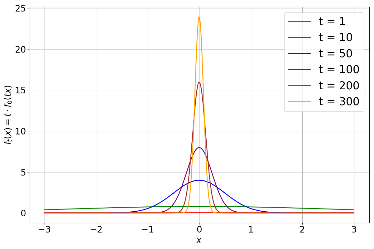
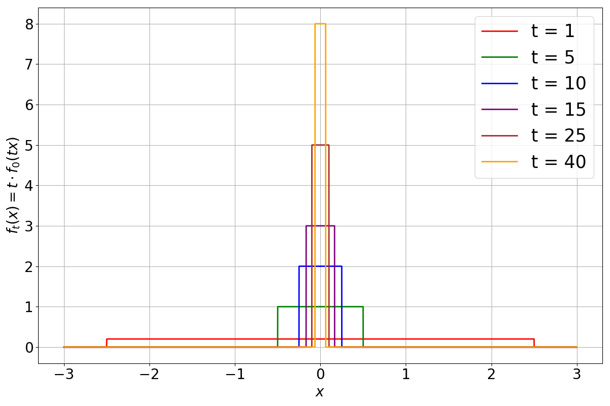
An important example of mappings that transform any function from F into a delta function, is the following
Here we take . Fig. 1 shows how this mapping translates the PDF of the normal distribution and the continuous uniform distribution as .
4.4 Analysis of Conjecture 1 (Khritankov, 2021)
In this Section, we investigate Conjecture 1 given by Khritankov (2021), which says that a positive feedback loop exists in system (1) if the operator is compressive in the metric space of the model predictions. However, this Conjecture was not proved in the original paper, we will give results that prove its correctness.
We now give a corollary of the Theorem 3, which will help us estimate the tendency of the moments of the random variables towards zero.
Lemma 1 (Decreasing moments).
If a system (1) with satisfies the conditions of the Theorem 3 and diverges to infinity, then all even moments of the random variable (if they exist) decrease with a speed of at least , that is , where is a -th moment on a step .
Discussion of Lemma 1.
Lemma 1 is interesting from a practical point of view, since calculations of moments of random variables are much easier to verify in a computational experiment than the conditions of Theorem 3.
This Lemma also helps in analysis of Conjecture 1 (Khritankov, 2021), since even moments, such as variance, can be considered as an indicator of predictions quality. Consequently, if there is a tendency towards a delta function, then the mapping is contractive in a vector space of regression quality metrics. But if sequence tends towards the delta function, then there is a positive feedback loop in our system (1), that is Conjecture 1 is true in this case.
The next lemma also attempts to analyse the Conjecture 1 in our formulation of the problem (1).
Lemma 2 (Inequality on ).
Consider a function
where is an arbitrary Lebesgue-measurable set of a non-path measure, —the measure of a set .
Then for all such that and for all such that the following inequality holds
Discussion of Lemma 2.
First of all, note that the result of Lemma 2 does not depend in any way on whether is a transformation on F or not, it is a consequence of Hölder’s inequality.
If we consider the problem statement from this paper, hence translates F into F, then the function is a PDF of vectors uniformly distributed on a set . Consequently, , that is from Lemma 2 we can only conclude that the norm of the operator is greater than or equal to one. But if , then would not be a contraction mapping in , because there would always be a function such that . This is important because if there is a tendency to zero distribution in our system, then the mappings would be contractions in any norm , that is .
4.5 Results for an Autonomous System (2)
Autonomy is an important property of any dynamical system. Such systems do not depend on the initial time from which the observation of this system started. Also, the Theorem 3 of this paper considers the tendency of time step to infinity, but in practice we can only consider finite . However, if the system is autonomous, we can study our system on a finite interval and understand its behavior at infinite .
From Theorem 3 we can see that there is a special kind of mappings (4) that bound the PDFs of our data from above, that is the mappings of this type that we will consider in this section. For such mappings we can derive an autonomy criterion for the system (2).
Theorem 4 (Autonomy criterion).
If the evolution operators of a dynamic system (1) have the form (4), then the system is autonomous if and only if
| (6) |
Discussion of Theorem 4.
This criterion is easy to check in practice, since the condition (6) means that the sequence is a power sequence, that is for some .
5 Experiments
The goal of our experiments is to compare the theoretical predictions given in Section 4 with actual measurements. In Section 5.1, we present two experiment designs: sliding window and sampling update. In Section 5.2, we describe an empirical study of the limit set of the system (1). Section 5.3 focuses on analysing the normality of the distribution of the training sample as time step tends to infinity. In Section 5.4, we check the predictions of Theorem 3 against measurements in one-dimensional case. In Section 5.5, we analyse the behavior of the system in the experiment design introduced earlier for autonomy using Theorem 4. Section 5 will be devoted to verifying Lemma 1 in practice.
5.1 Experiment Design
We conduct several experiments to test theoretical predictions we devised in the previous section. The goal of these experiments is to compare the predictions with the actual observations in a controlled environment.
Here is a formal statement of a exemplary problem to demonstrate the repeated learning process. Following the problem statement (1), let F (3) be a space of probability density functions. At step we take the initial and sample an original set of size from and take as normally distributed noise. We consider a regression problem with a loss function , that is find such that
In order to explore how regularization, cross-validation and learning algorithms affect the theoretical results, we use a linear regression model without regularization learned with an SGD algorithm with the maximum number of iterations equal to 50, a Ridge regression model without any regularization and solve it in closed-form using Cholesky decomposition, and RidgeCV regression model with the regularization parameter equal to solved using SVD. Models and learning algorithms are implemented in the Scikit-learn library (Pedregosa et al., 2011).
We take synthetic initial data sets in order to limit unknown confounding factors and isolate the effect of the repeated learning. In the first data set, input data X is normally distributed and is a linear function of X with additional normal noise. As the second data set we take Friedman problem (Friedman, 1991), which is not linear. Both of these data sets are obtained from the Scikit-learn library (Pedregosa et al., 2011) using make_regression() and make_friedman1() routines. The number of objects in the data set X equals and the number of features is . At step the input data in both cases is i.i.d., relation between X and is linear in the first case. We run each experiment ten times to reduce the randomness.
We employ MLDev reproducible experiments toolkit (Khritankov et al., 2021) to implement the simulation environment. The source code and initial data to reproduce the experiments can be found in the Gitlab repository 111Source code for the experiments: https://gitlab.com/repeated_ml/dynamic-systems-model.
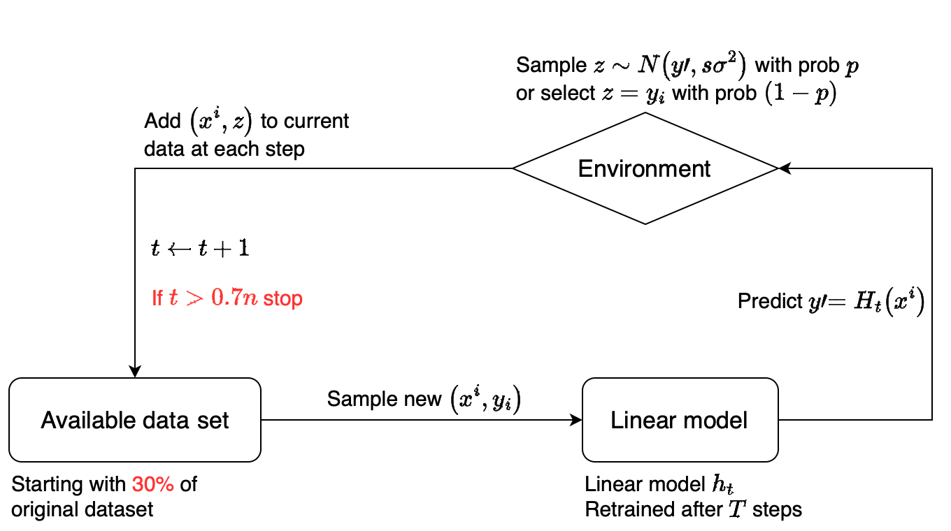
In the sliding window update experiment setting (Khritankov, 2023), at round we first sample of the original data X on which our model is trained on a subset of input data. Then, at each step , we randomly sample without replacement an item —the features and target variable of the item from the remaining data. Next, we obtain the prediction from the model and sample , where is adherence (Khritankov, 2023), a parameter of the experiment, and is the mean squared error of the predictions on the held-out subset of the current set of step . After that, we evict the earliest item from the current set and append the new item with usage (Khritankov, 2023) probability or item with probability . We repeat the procedure until we run out of items in the original set, making a total of steps. After every steps, is increased: and the machine learning model is retrained with a training size of on the active set.
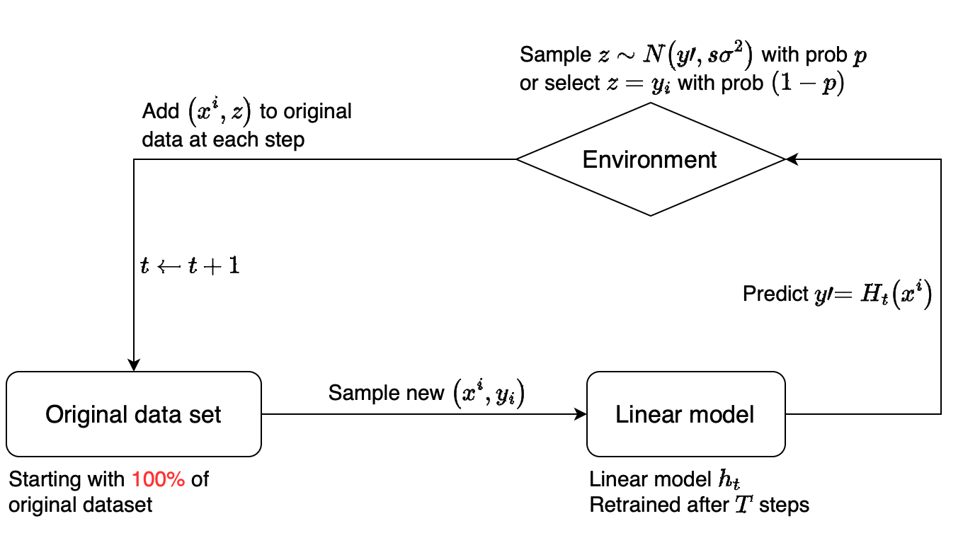
In the sampling update setting, the model is trained on the entire sample X at round . Then the procedure is very similar to the sliding window update, but when we take the element from the original set, we replace it using the same rules as in the sliding window setting. The consequence of such change is, first, that in the sampling update setting, the system would be autonomous as the procedure, and therefore the evolution operator D, do not depend on step . Second, is that we can run the sampling update experiment for unlimited time steps, whereas the sliding window experiment allows for only a maximum of iterations.
In both cases the size of the sliding window remains constant– for both the sliding window update and for the sampling update. Indeed, at each step we remove one item and add one item to the current set. The mapping transforms at each step , thus there exists an for the current set. As we compute only on the data from the data set, only the distribution of the target variable changes.
The schemes of the experiments are shown at Fig. 2.
5.2 Analysis of Prediction Error
According to Theorem 3 the two possible limiting distributions of are delta function or zero distribution . In this experiment we explore how the standard deviation of the prediction error changes over time. Based on Lemma 1 and Theorem 3, we should observe two cases in this experiment: the tendency of the variance to zero (that is, the tendency of the PDFs to the delta function) or the tendency of the variance to infinity (that is, the tendency of the PDFs to the zero distribution). For this reason, at every steps we calculate the standard deviation of the difference .
We run the experiment for different usage (Khritankov, 2023) values —what portion of the predictions are seen by the users, the probability with which we include in the current set, and adherence —how closely the predictions of the model are followed by the users, the parameter to multiply when sampling . We also vary the variance in the normal distribution of the noise : and . Fig. 3 shows only the result with noise variance , the picture is similar for other values. More figures can be found in the experiment repository. In this experiment we consider SGD regression model and synthetic linear data set.
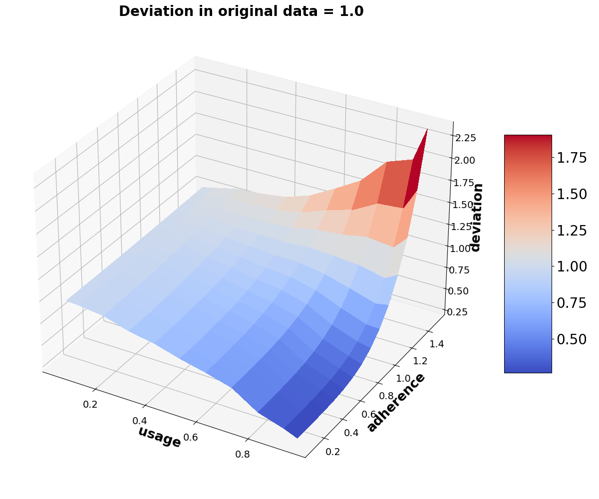
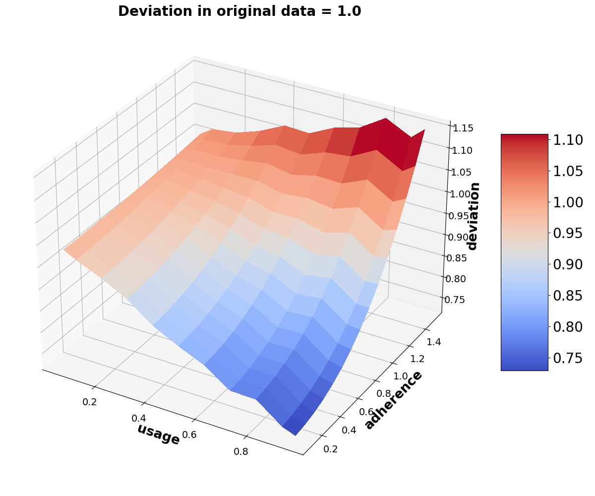
As we can see from Fig. 3, as usage increases and adherence (Khritankov, 2023) decreases, the deviation decreases, because we start to add less noisy data to the current set.
In almost all cases explored the response surface shown at Fig. 3 is either of red or blue color, that is for most of the usage and adherence combinations there is a tendency towards either the delta or the zero function.
5.3 Normality Test for the Prediction Error
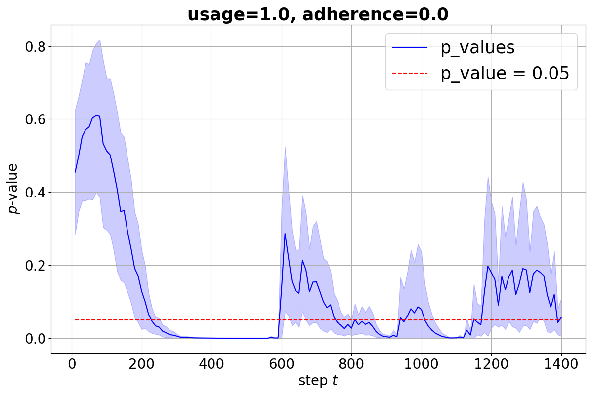
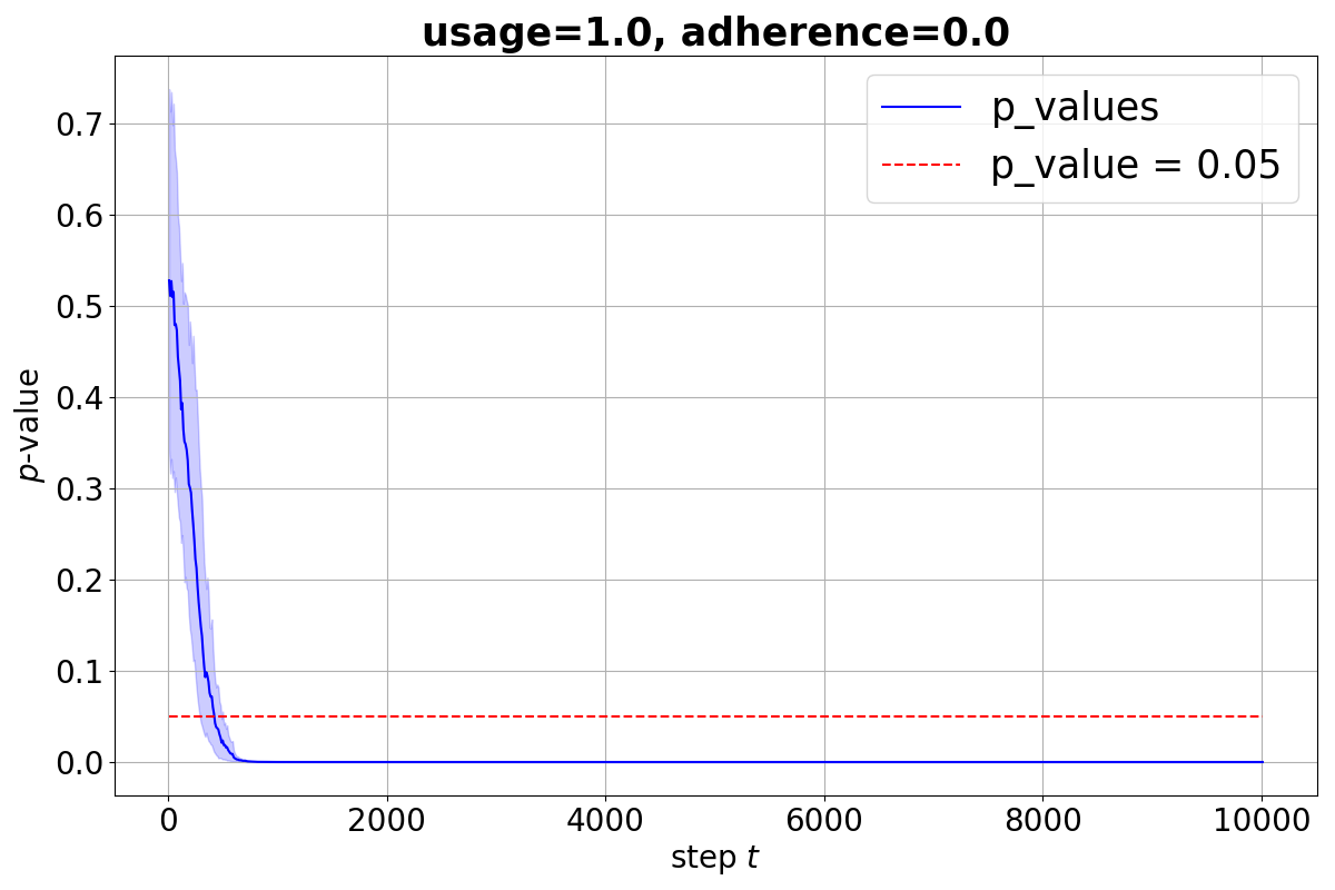
In this experiment we consider a linear regression model with squared loss and synthetic linear data set. Because the original training data is normally distributed and is relates with X linearly, it is feasible to check prediction error for normality. In this experiment we explore how the probability density of the data changes as a result of the feedback loop.
We use D’Agostino and Pearson’s test for normality and calculate the -value. Here we take usage and adherence values from on the previous Experiment 5.2: and , and , and correspondingly.
As we can see from the measurements, the original data is normally distributed with -value larger than the threshold. However, subsequently the -value decreases and the normality of the sampled data at step breaks down. The -values become very close to zero and mostly lower than the chosen threshold as time step progresses. We may conclude from the histogram that a possible reason for this is that distribution of is a mixture of the two or more normal probability distributions.
5.4 Limit to Delta Function or Zero Distribution
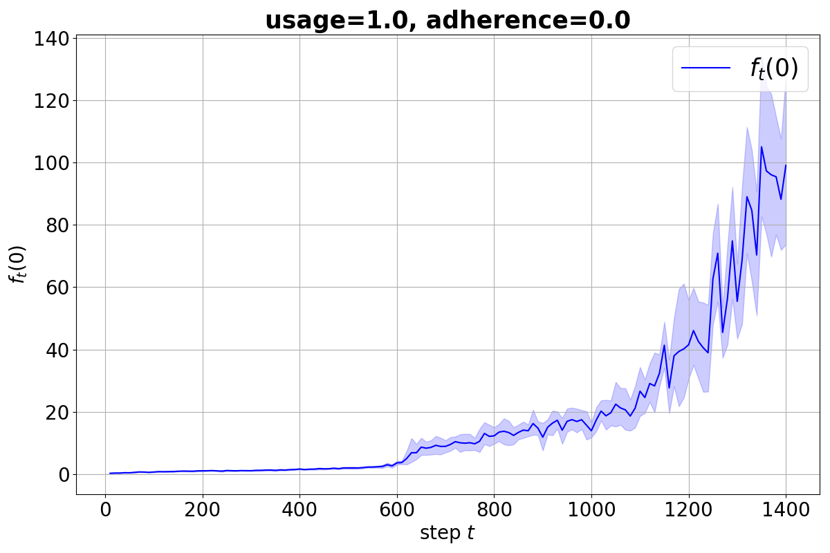
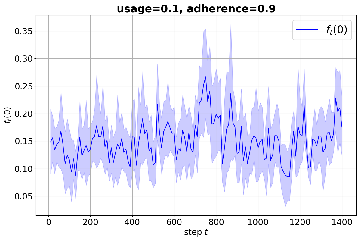
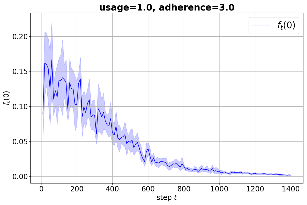
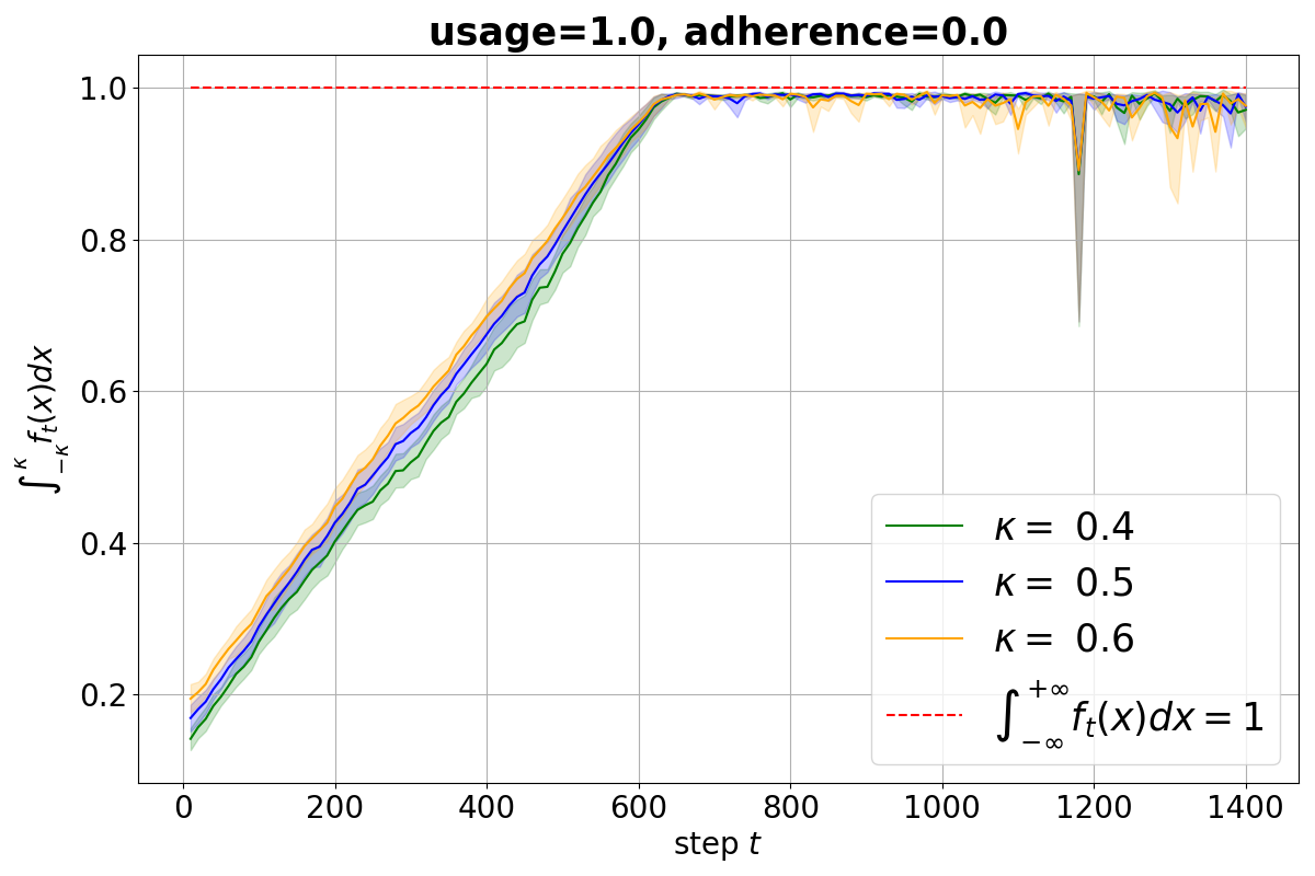
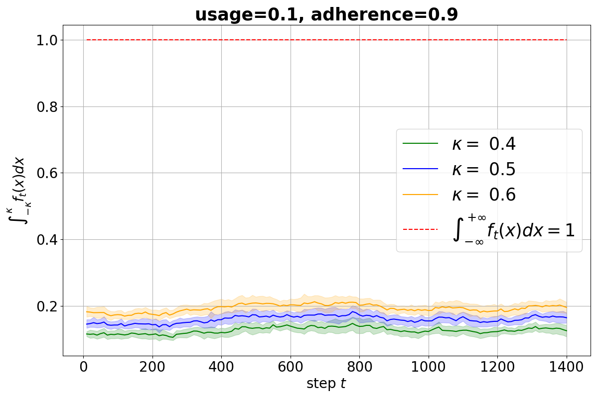
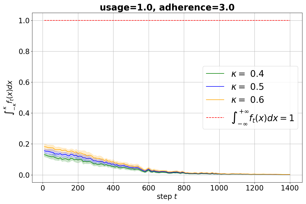
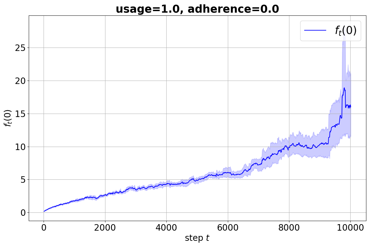
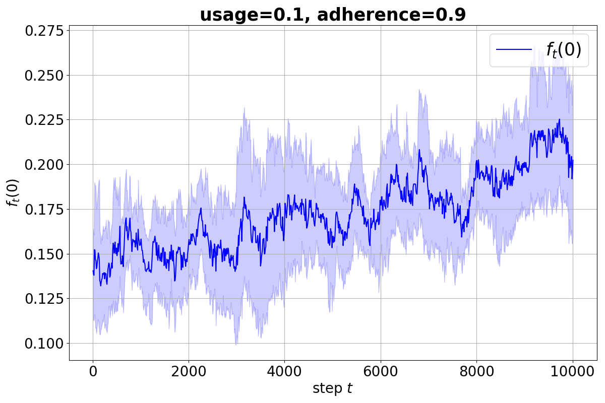
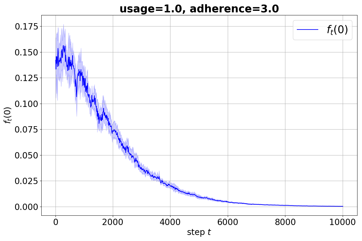
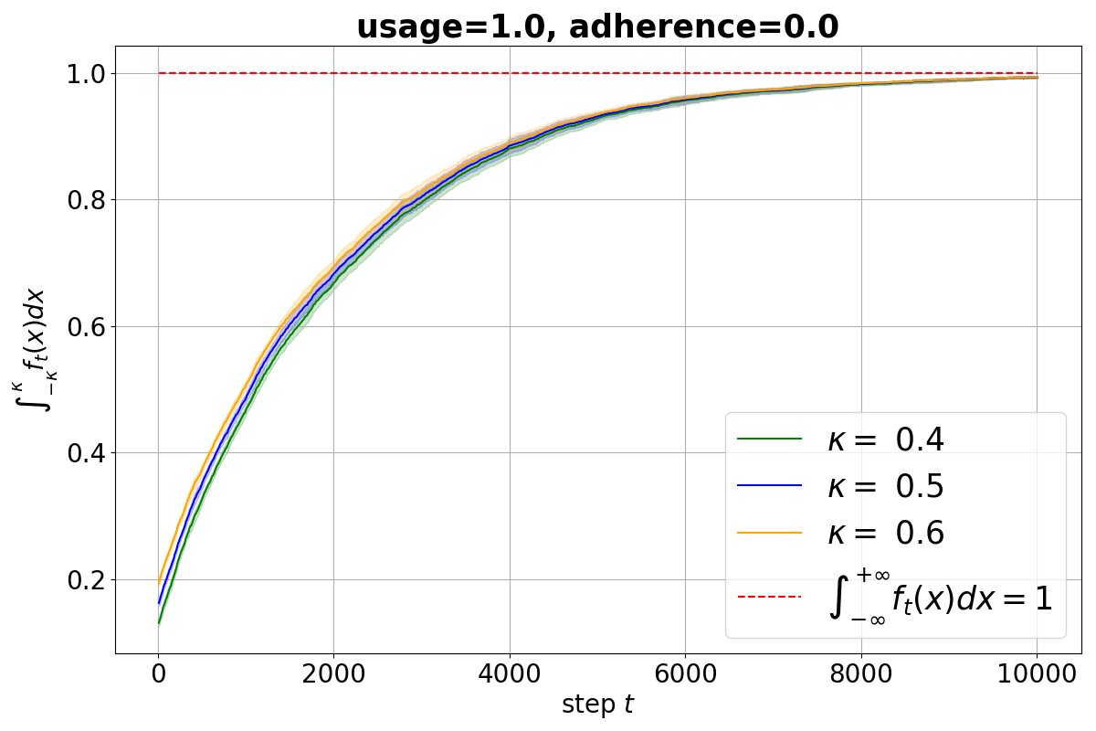
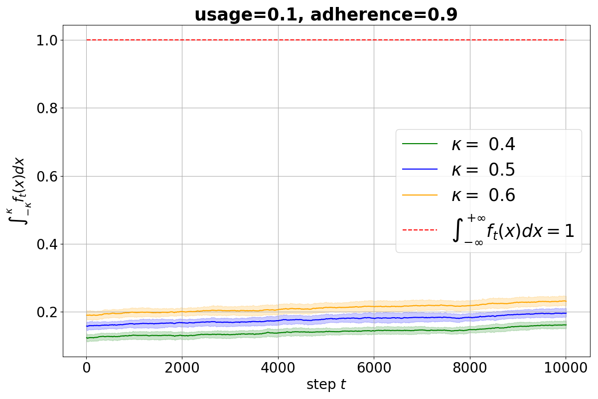
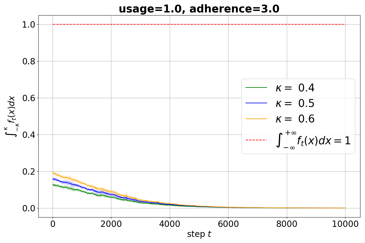
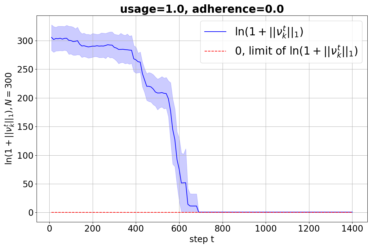
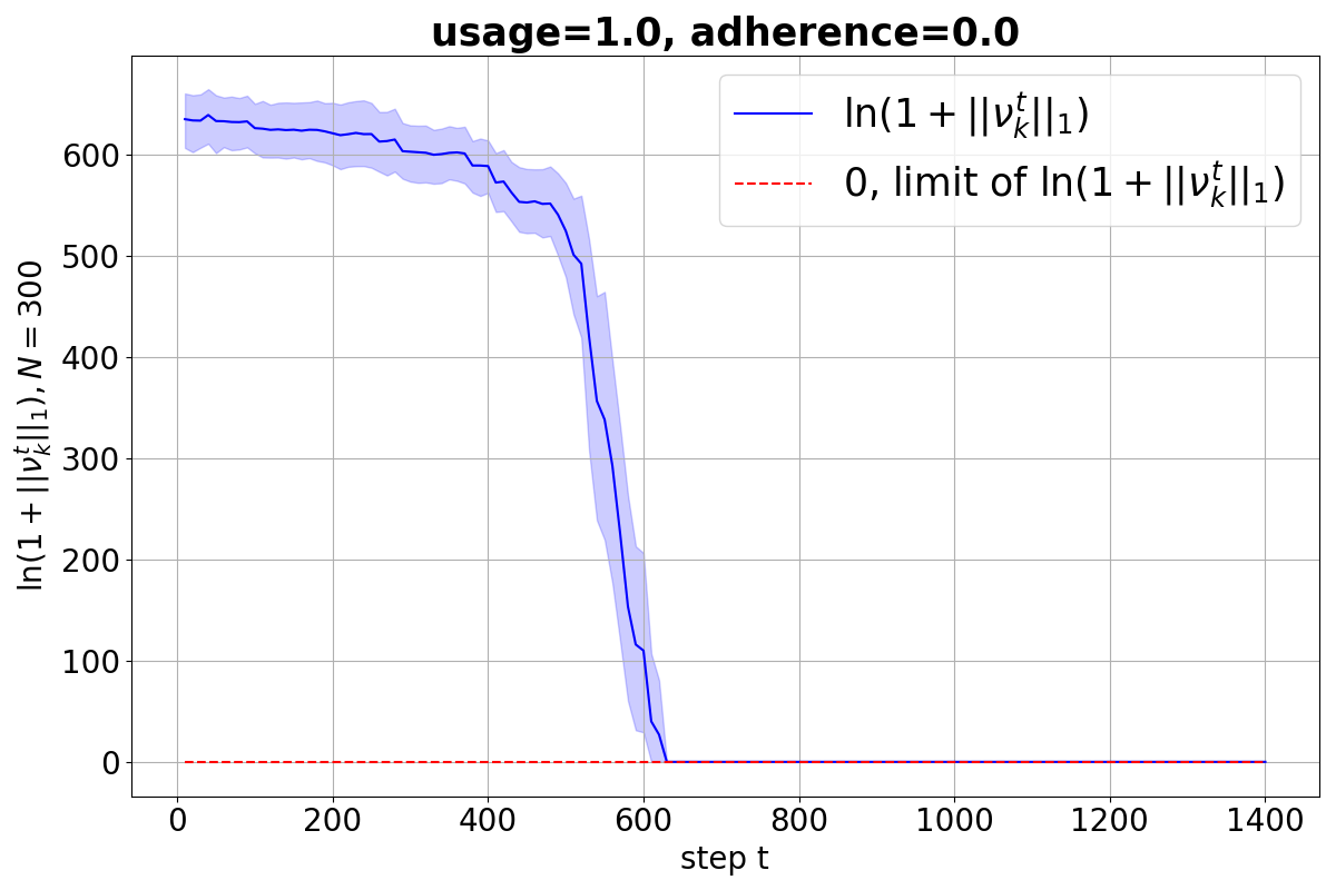
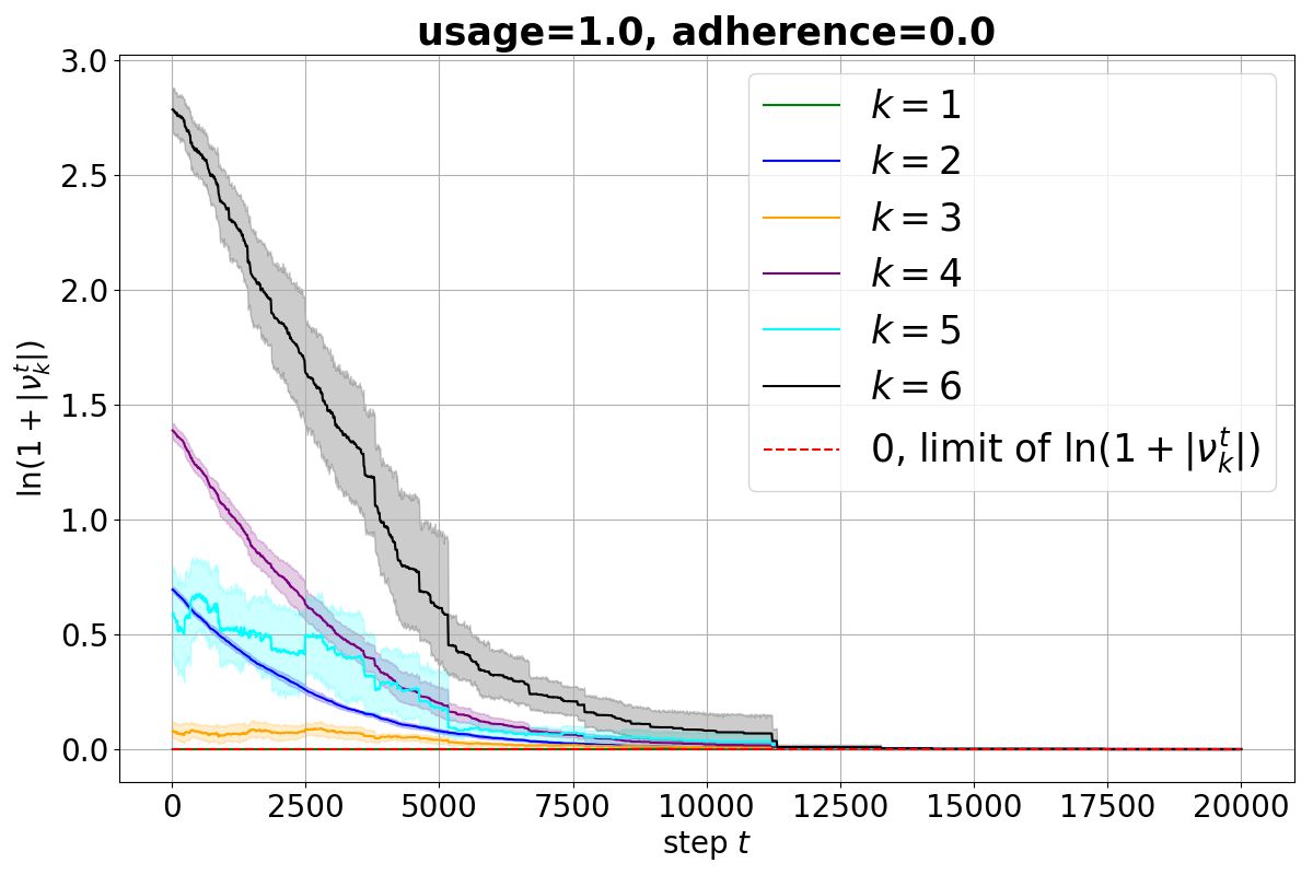
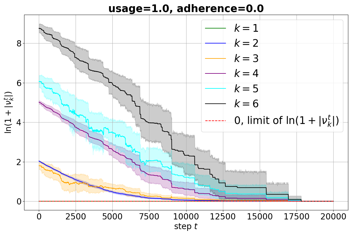
In this experiment we directly test the predictions of Theorem 3, that is we measure and , where is sufficiently small. We estimate using a more numerically stable linear interpolation heuristic method from the SciPy library (Virtanen et al., 2020) that gives results close to theoretically grounded density estimation (Silverman, 1986) method. The data collected in this experiment are shown at Fig. 4 and Fig. 5. In this experiment we consider SGD regression model on synthetic linear data set and Ridge model with no regularization on Friedman data set.
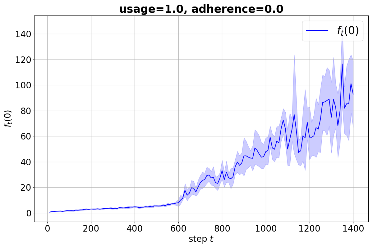
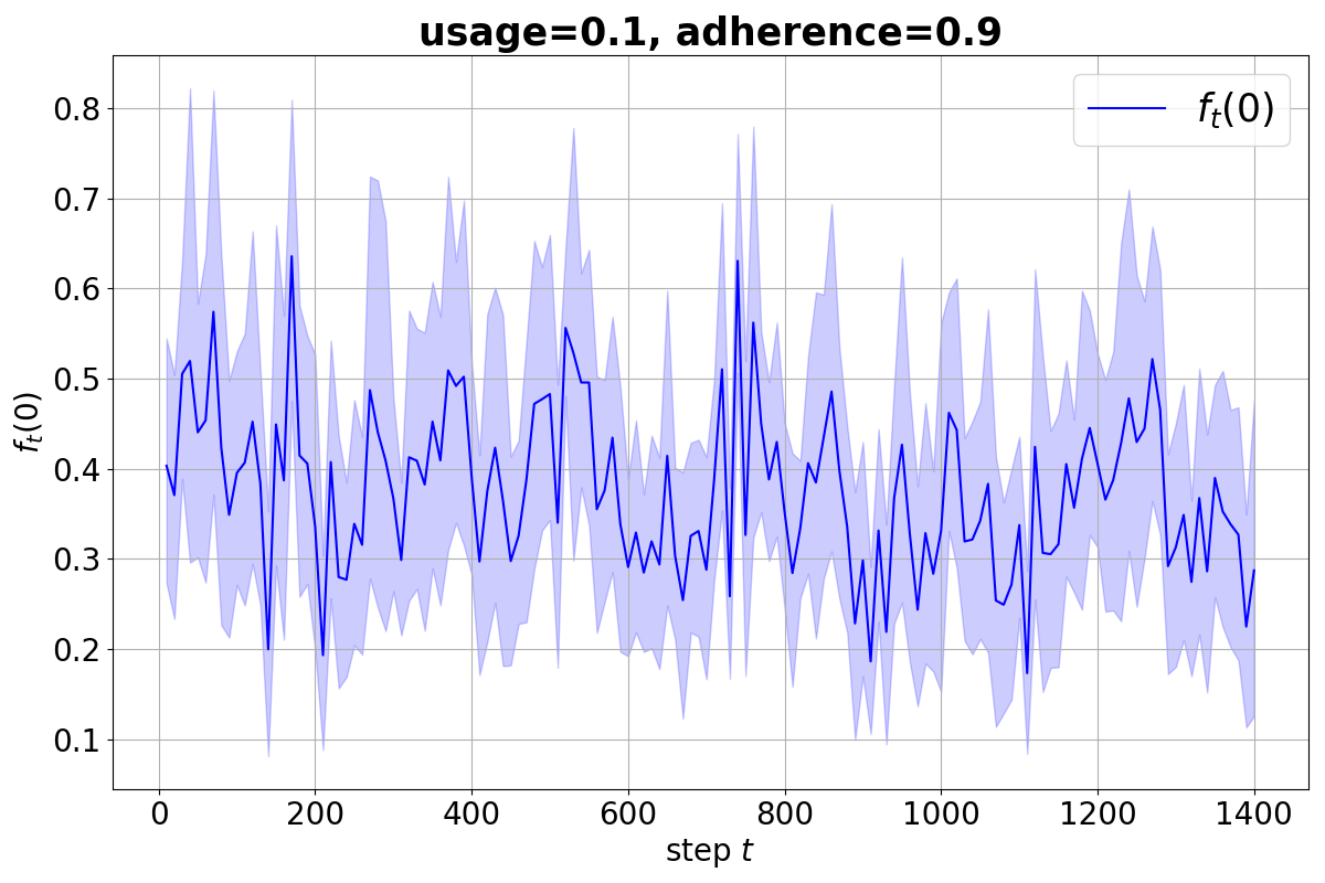
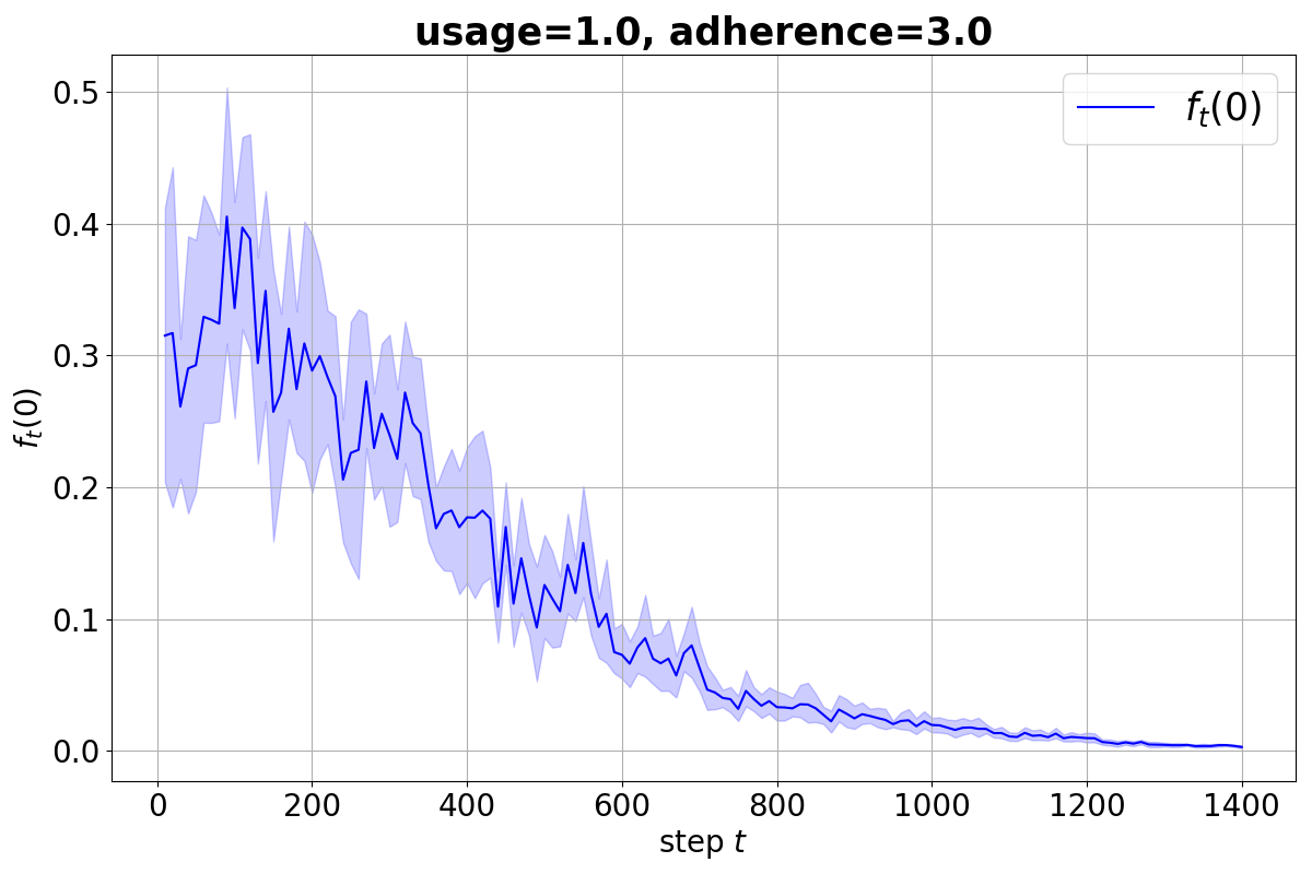
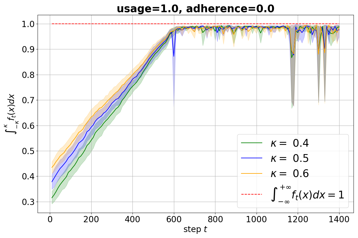
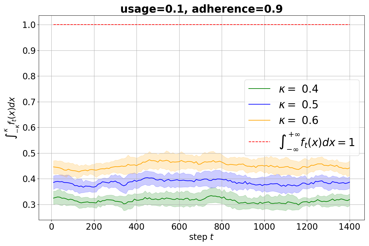
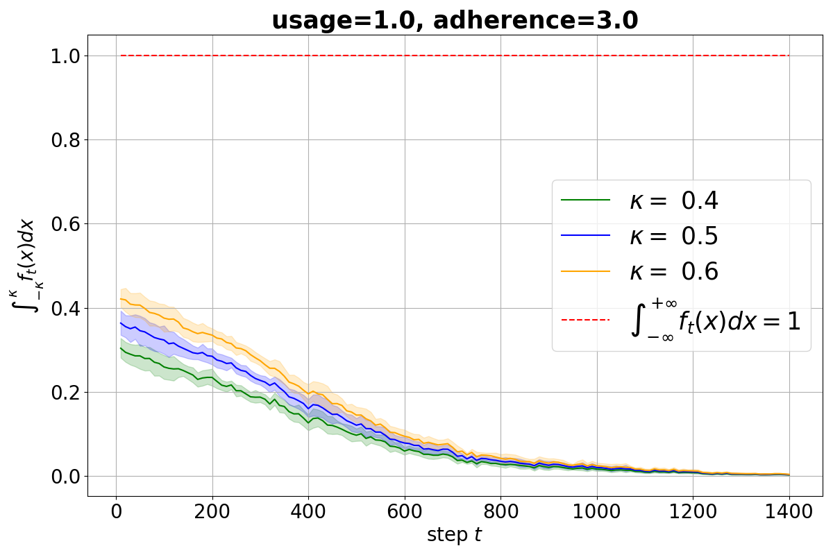
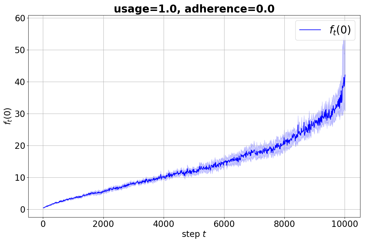
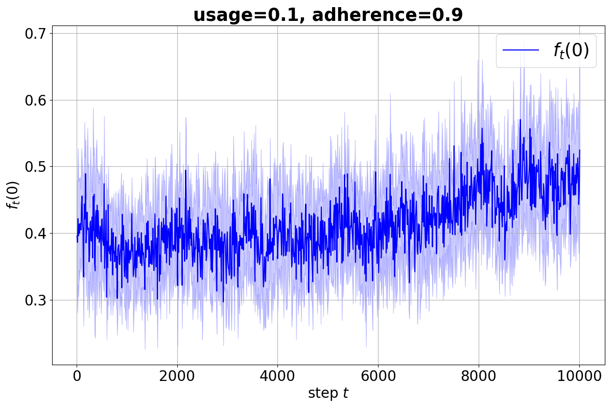
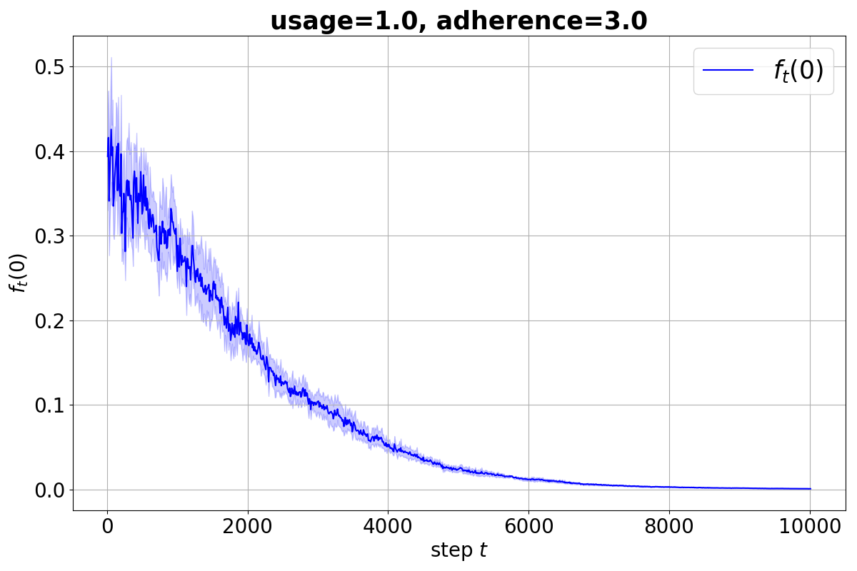
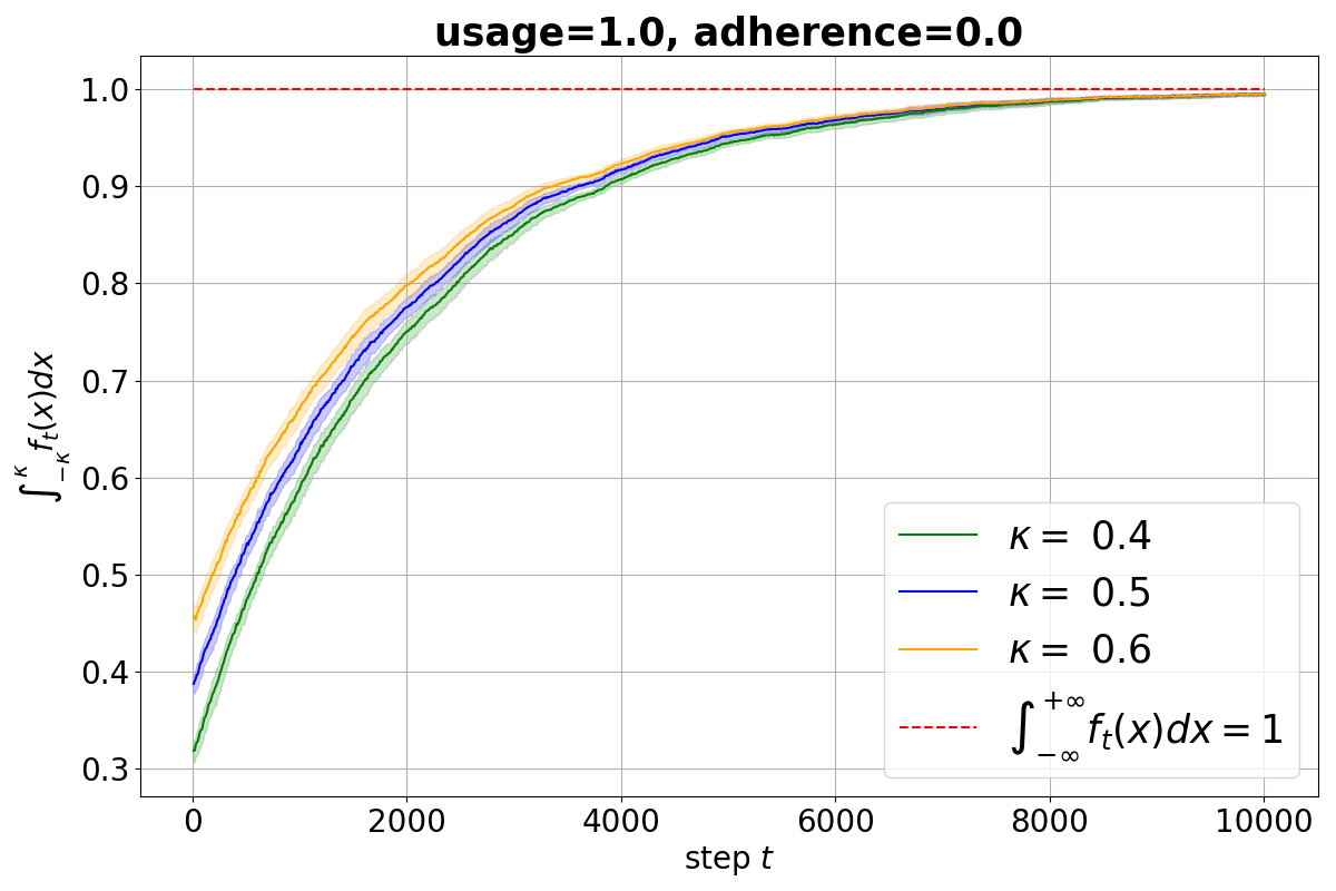
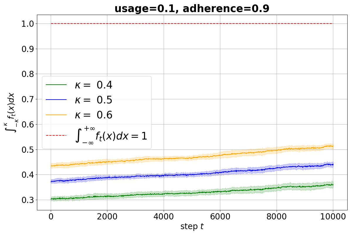
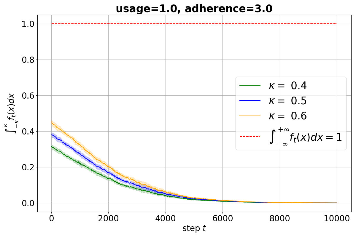
As we can see, if usage and adherence , the limiting probability density of , that is the probability density of , is zero distribution . This corresponds to the fact that tends to zero and tends to zero. When usage and adherence we observe a tendency to the delta function , that is tends to positive infinity and tends to one. If usage and adherence , the probability density of remains almost the same, that is tends to some constant .
Therefore, we can conclude that the observed behavior does not contradict the claims of Theorem 3.
5.5 Autonomy check
We test the claim (6) of Theorem 4. According to the discussion of Theorem 4, for the sequence to satisfy the condition (6), it must be a power sequence.
In this experiment, we assess the autonomy of the exemplary machine learning systems in the sliding window update and sampling update settings. The former is not autonomous and the latter is an autonomous system by construction, because the evolution operator , that is the learning algorithm and feedback procedure, does not depend on time step, . We plot and check if there is a straight line when the system is autonomous, or not a straight line for a non-autonomous system. For clarity, we fit a linear model to the measurements and show the score—a statistical measure of how well the line matches the data. The observations and the lines are shown at the Fig. 6-9. We provide the results for SGD and RidgeCV regression models on synthetic linear and Friedman data sets.
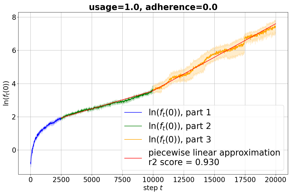
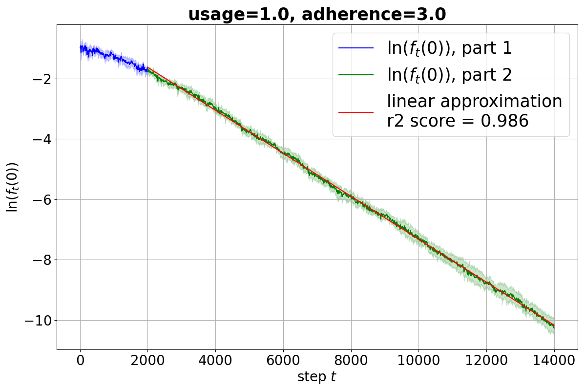
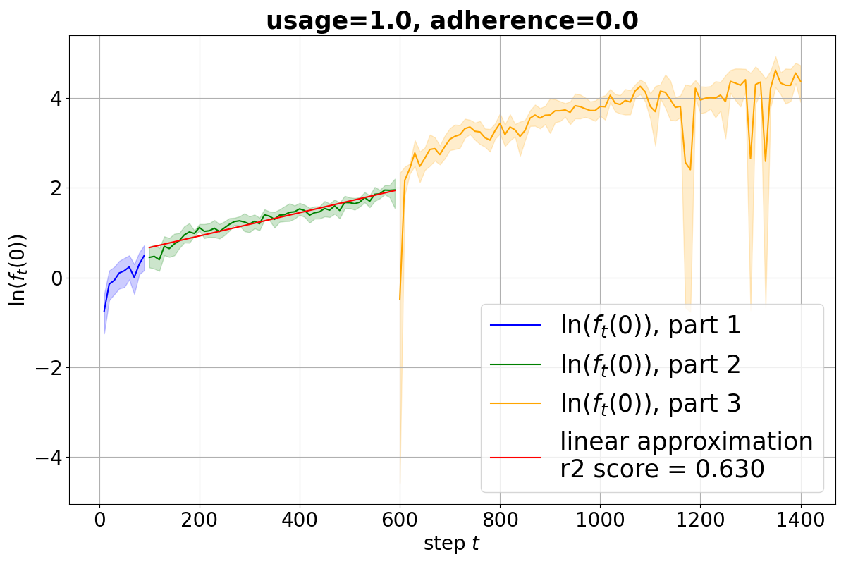
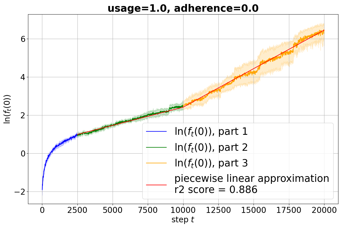
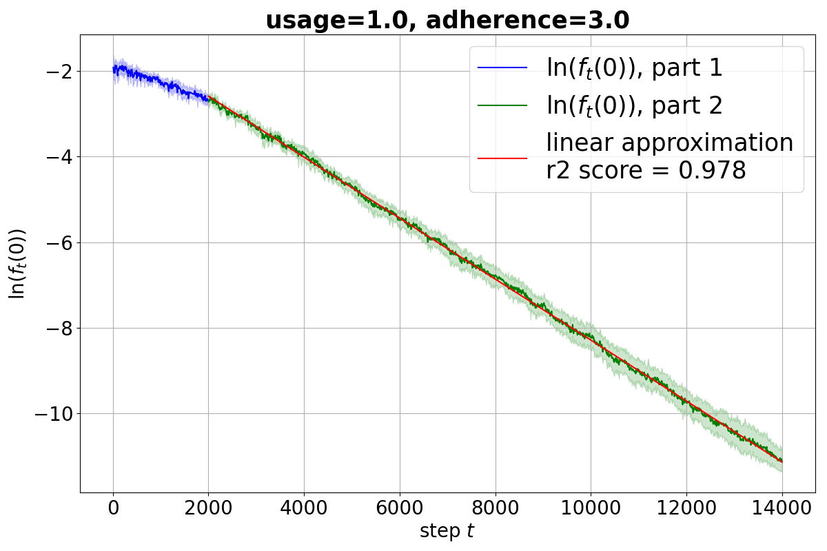
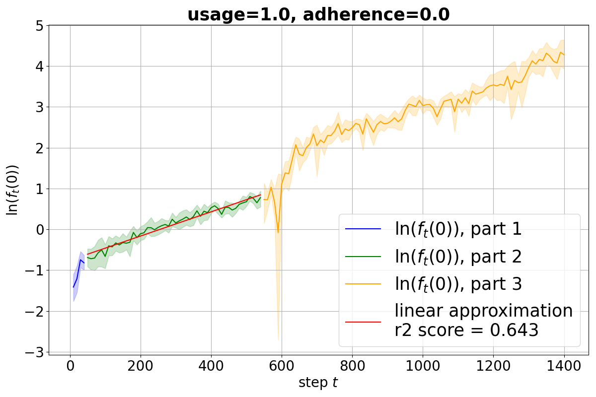
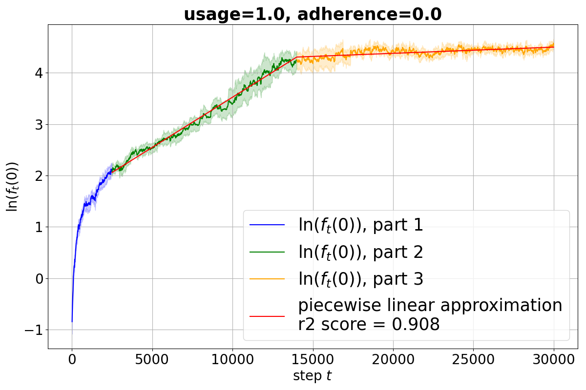
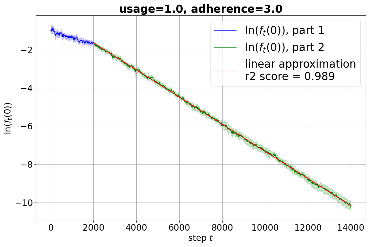
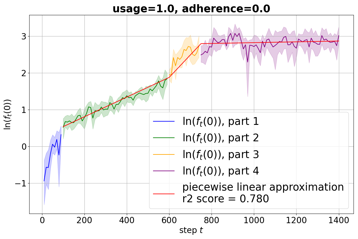
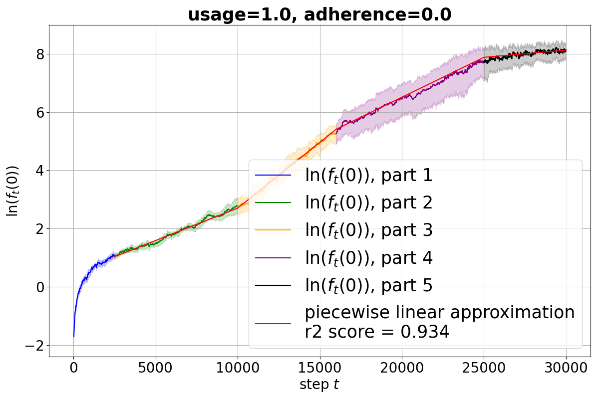
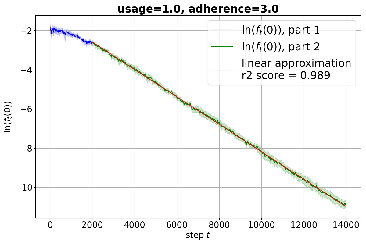
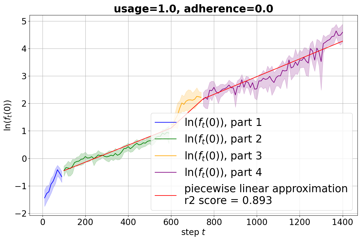
As you can see, in case of the sliding window update we obtain a poor fit on all models and data sets, so the system is not autonomous. On the figure there is a notable change in around , this corresponds to the point where the proportion of reused predictions in the data stabilizes at usage rate does not change any further. The sampling update setup in case of usage and adherence is autonomous on all models and data sets, since there is a good fit. In case of usage and adherence we observe two linear segments, except in the case of RidgeCV on the Friedman data set. While our hypothesis states there should be just one linear segment, we may see two regions of autonomy. We contemplate that this may be due to the fact that at all the items in the original i.i.d. data set are replaced by the model predictions.
In order to solve the aforementioned regression problem to obtain the fit, we use the robust Huber regressor. We also perform a Breusch-Pagan Lagrange multiplier test for homoscedasticity (d’Agostino, 1971). In the sampling update case we get a -value of and in the sliding window case the -value equals to . Therefore, we assume that the residuals in all cases are homoscedastic and the fit is justified.
With this we may conclude that the claims of Theorem 4 does not contradict to the observations in this experiment. The hypotheses about the autonomy of the two systems are partially confirmed.
5.6 Decreasing Moments
In this experiment we compare the predictions of Lemma 1 with the observations. In the sliding window update setting we check the third term of this Lemma: . For computational efficiency reasons, we report only for .
In the sampling update experiment setting we check the second claim of the Lemma, that is for . The observations for this experiments are shown at Fig. 10 and Fig. 11. All the results in this experiment are for SGD regression model on synthetic linear and Friedman data sets.
As we can see from the measurements, the second and third claims of Lemma 1 are satisfied in all observed cases. When usage and adherence the limit of mappings , and correspondingly of , is the delta function . However, we do not get exactly zero, as the plot may show, since in all cases we consider only finite .
6 Limitations and Threats to Validity
Threats to internal validity relate to how the experimental design and other internal factors affect the study we are conducting. The mathematical formulation of the repeated machine learning (1) describes a broad class of problems. The theory we develop places such constraints on the mappings and that are satisfied in most practical applications. However, in our experiments we only test the theoretical predictions for two synthetic data sets with additive noise, and three linear regression models and learning algorithms. Results of the experiments depend on the model and the data set we use. Another problem could be the imperfection of the Python language and the modeling environment we use. In the Experiment 5.4 we measure and observe distortions in the plot at larger values of step (see Fig. 4, Fig. 5), which may be caused by rounding errors and approximation errors between the true probability density function and the empirical density function (4.2).
Threats to construct validity relate to the correspondence between theoretical predictions and what is observed in the experiment. In Experiment 5.4 we study the convergence of sequences of density functions to the zero distribution (see Fig. 4 and Fig. 5). We take the integral , but in general the functions can tend to a non-zero value somewhere outside the interval . In practice it is very difficult to choose a neighbourhood of infinity, therefore we choose several values for and check that for all of them the integral tends to zero as the step increases.
Threats to conclusion validity relate to the correspondence between theory and result. When testing our system for autonomy in Experiment 5.5, we check whether the score for a trend line is small enough to have follow a straight line with step . We conclude that one of the designs is autonomous and the other is not from this test. However, there is no clear bound on score at which the graph can be recognised as not a straight line. Moreover, in our theoretical predictions the step tends to infinity, while in practice we take only finite . In the sliding window experiment (see Fig. 2) we take step because the process has to stop by construction after that. In the sampling update experiment we take , as we consider this number of steps sufficient. In the norm test of the tendency of moments to zero in Experiment 5.6 we cannot compute an infinite sum of moments either, therefore we limit ourselves to the first moments assuming that the remaining higher moments do not contribute a lot.
Threats to external validity relate to the differences between the simulation environment and real systems. We propose two experiment designs that are strong simplifications of repeated machine learning systems. For example, in the real-world systems, a user may or may not adhere to the predictions of the system with a non-variable probability of use. In addition, user adherence may change over time, or the decision to adhere may depend on the model’s predictions in more complex ways, such that the linear approximation we make in Section 5 does not hold. We could give much more examples of how the described schemes of repeated machine learning process do not correspond to reality, but since the purpose of our experiments is to verify the theoretical results, these simulations are sufficient for the goals of the current research.
7 Conclusion
The problem of repeated machine learning we study is very important because a machine learning algorithm is almost always part of a larger software system and interacts with the environment of the system. It is important to understand how this interaction happens, how it changes the quality characteristics of the machine learning system, and are there any violations of the trustworthiness requirements.
In this paper we apply the apparatus of discrete dynamical systems, mathematical analysis and probability theory to build a theoretical framework to state and solve the problem of repeated supervised learning. We correspond a machine learning system operating in its context of use with a dynamical system defined by the evolutionary mapping (1). Theorem 3 gives us the understanding of how this mapping transforms the initial data distribution and what is the limiting distribution: a delta function or a zero distribution. From this result we can judge whether a positive feedback loop exists and produces a concept drift, or a negative loop is present and degrades the prediction performance of the system.
We also prove Theorem 4 and Lemma 1 using results from Theorem 3. Theorem 4 is the criterion of the autonomy of our dynamical system, a useful property for the further analysis. Lemma 1 is about the tendency to zero moments of the residuals in a positive feedback loop. These results, unlike the statements of the Theorem 3, are easier to verify experimentally, which makes them useful in practical applications.
We develop a simulation environment in the Python language for the repeated supervised learning process, and demonstrate the effects of repeated machine learning in two settings: sliding window update and sampling update (see Fig. 2). Both settings are reusable for any other experiments involving repeated machine learning. As shown in Experiment 5.5, the sampling update setting is autonomous, while the sliding window update setting is not.
All the results we obtain are strongly proven and tested in computational experiments. Our assumptions turned out to be correct, the practical results agree with the theory.
Expanding on the ideas in this paper is important for developing machine learning systems and its applications. Future research may include more experiments on real-world data sets and more complex models. In the experiments and in the discussion of Theorem 3, we do not consider deriving the envelope function . Perhaps, future studies should be devoted to its construction. Another direction for future research could be to endow the set F with a metric like Kullback-Leibler metric and analyse mappings in this metric space.
References
- Adam et al. (2020) George Alexandru Adam, Chun-Hao Kingsley Chang, Benjamin Haibe-Kains, and Anna Goldenberg. Hidden risks of machine learning applied to healthcare: unintended feedback loops between models and future data causing model degradation. In Machine Learning for Healthcare Conference, pages 710–731. PMLR, 2020.
- Adam et al. (2022) George Alexandru Adam, Chun-Hao Kingsley Chang, Benjamin Haibe-Kains, and Anna Goldenberg. Error amplification when updating deployed machine learning models. In Machine Learning for Healthcare Conference, pages 715–740. PMLR, 2022.
- Bernard et al. (2022) Pauline Bernard, Vincent Andrieu, and Daniele Astolfi. Observer design for continuous-time dynamical systems. Annual Reviews in Control, 53:224–248, 2022. ISSN 1367-5788. doi:10.1016/j.arcontrol.2021.11.002.
- CAIS (2023) CAIS. Statement on AI Risk. https://www.safe.ai/statement-on-ai-risk, 2023. Accessed: 2023-09-03.
- Cheng et al. (2021) Lu Cheng, Kush R Varshney, and Huan Liu. Socially responsible AI algorithms: Issues, purposes, and challenges. Journal of Artificial Intelligence Research, 71:1137–1181, 2021. doi:10.1613/jair.1.12814.
- Chouldechova and Roth (2020) Alexandra Chouldechova and Aaron Roth. A snapshot of the frontiers of fairness in machine learning. Commun. ACM, 63(5):82–89, apr 2020. ISSN 0001-0782. doi:10.1145/3376898.
- d’Agostino (1971) Ralph B d’Agostino. An omnibus test of normality for moderate and large size samples. Biometrika, 58(2):341–348, 1971.
- Davies (2018) Huw C Davies. Redefining filter bubbles as (escapable) socio-technical recursion. Sociological Research Online, 23(3):637–654, 2018. doi:10.1177/1360780418763824.
- Dvoretzky et al. (1956) Aryeh Dvoretzky, Jack Kiefer, and Jacob Wolfowitz. Asymptotic minimax character of the sample distribution function and of the classical multinomial estimator. The Annals of Mathematical Statistics, pages 642–669, 1956.
- Ensign et al. (2018) Danielle Ensign, Sorelle A Friedler, Scott Neville, Carlos Scheidegger, and Suresh Venkatasubramanian. Runaway feedback loops in predictive policing. In Conference on fairness, accountability and transparency, pages 160–171. PMLR, 2018.
- Feller (1991) William Feller. An introduction to probability theory and its applications, Volume 2, volume 81. John Wiley & Sons, 1991. doi:10.1063/1.3034322.
- Friedman (1991) Jerome H Friedman. Multivariate adaptive regression splines. The annals of statistics, 19(1):1–67, 1991.
- Galor (2007) Oded Galor. Discrete dynamical systems. Springer Science & Business Media, 2007. doi:10.1007/3-540-36776-4.
- He et al. (2021) Hongmei He, John Gray, Angelo Cangelosi, Qinggang Meng, T Martin McGinnity, and Jörn Mehnen. The challenges and opportunities of human-centered AI for trustworthy robots and autonomous systems. IEEE Transactions on Cognitive and Developmental Systems, 14(4):1398–1412, 2021. doi:10.1109/TCDS.2021.3132282.
- Itoh (1979) Shigeru Itoh. Random fixed point theorems with an application to random differential equations in banach spaces. Journal of Mathematical Analysis and Applications, 67(2):261–273, 1979. ISSN 0022-247X. doi:https://doi.org/10.1016/0022-247X(79)90023-4. URL https://www.sciencedirect.com/science/article/pii/0022247X79900234.
- Katok and Hasselblatt (1995) Anatole Katok and Boris Hasselblatt. Introduction to the modern theory of dynamical systems. Cambridge university press, 1995. doi:10.3934/dcds.2013.33.1451.
- Khritankov (2021) Anton Khritankov. Hidden feedback loops in machine learning systems: A simulation model and preliminary results. In Software Quality: Future Perspectives on Software Engineering Quality: 13th International Conference, SWQD 2021, Vienna, Austria, January 19–21, 2021, Proceedings 13, pages 54–65. Springer, 2021. doi:10.1007/978-3-030-65854-0_5.
- Khritankov (2023) Anton Khritankov. Positive feedback loops lead to concept drift in machine learning systems. Applied Intelligence, pages 1–19, 2023. doi:10.1007/s10489-023-04615-3.
- Khritankov and Pilkevich (2021) Anton Khritankov and Anton Pilkevich. Existence conditions for hidden feedback loops in online recommender systems. In Web Information Systems Engineering–WISE 2021: 22nd International Conference on Web Information Systems Engineering, WISE 2021, Melbourne, VIC, Australia, October 26–29, 2021, Proceedings, Part II 22, pages 267–274. Springer, 2021. doi:10.1007/978-3-030-91560-5_19.
- Khritankov et al. (2021) Anton Khritankov, Nikita Pershin, Nikita Ukhov, and Artem Ukhov. Mldev: Data science experiment automation and reproducibility software. In International Conference on Data Analytics and Management in Data Intensive Domains, pages 3–18. Springer, 2021. doi:10.1007/978-3-031-12285-9_1.
- Li et al. (2023) Bo Li, Peng Qi, Bo Liu, Shuai Di, Jingen Liu, Jiquan Pei, Jinfeng Yi, and Bowen Zhou. Trustworthy AI: From principles to practices. ACM Computing Surveys, 55(9):1–46, 2023. doi:10.1145/3555803.
- Michiels et al. (2022) Lien Michiels, Jens Leysen, Annelien Smets, and Bart Goethals. What are filter bubbles really? a review of the conceptual and empirical work. In Adjunct Proceedings of the 30th ACM Conference on User Modeling, Adaptation and Personalization, pages 274–279, 2022. doi:10.1145/3511047.3538028.
- Milnor (1978) John Milnor. Analytic proofs of the “hairy ball theorem” and the brouwer fixed point theorem. The American Mathematical Monthly, 85(7):521–524, 1978. doi:10.1080/00029890.1978.11994635.
- Nemytskii (2015) Viktor Vladimirovich Nemytskii. Qualitative theory of differential equations, volume 2083. Princeton University Press, 2015. doi:10.1515/9781400875955.
- Ouannas et al. (2017) Adel Ouannas, Ahmad Taher Azar, and Sundarapandian Vaidyanathan. On a simple approach for qs synchronisation of chaotic dynamical systems in continuous-time. International Journal of Computing Science and Mathematics, 8(1):20–27, 2017. doi:10.1504/IJCSM.2017.083167.
- Pedregosa et al. (2011) F. Pedregosa, G. Varoquaux, A. Gramfort, V. Michel, B. Thirion, O. Grisel, M. Blondel, P. Prettenhofer, R. Weiss, V. Dubourg, J. Vanderplas, A. Passos, D. Cournapeau, M. Brucher, M. Perrot, and E. Duchesnay. Scikit-learn: Machine learning in Python. Journal of Machine Learning Research, 12:2825–2830, 2011.
- Pei et al. (2022) Zhongyi Pei, Lin Liu, Chen Wang, and Jianmin Wang. Requirements engineering for machine learning: a review and reflection. In 2022 IEEE 30th International Requirements Engineering Conference Workshops (REW), pages 166–175. IEEE, 2022. doi:10.1109/REW56159.2022.00039.
- Sandefur (1990) James T Sandefur. Discrete dynamical systems: Theory and applications. Clarendon Press, 1990.
- Serban et al. (2021) Alex Serban, Koen van der Blom, Holger Hoos, and Joost Visser. Practices for engineering trustworthy machine learning applications. In 2021 IEEE/ACM 1st Workshop on AI engineering-software engineering for AI (WAIN), pages 97–100. IEEE, 2021. doi:10.1109/WAIN52551.2021.00021.
- Sharma et al. (2015) Puneet Sharma et al. Uniform convergence and dynamical behavior of a discrete dynamical system. Journal of Applied Mathematics and Physics, 3(07):766, 2015. doi:10.4236/jamp.2015.37093.
- Siebert et al. (2020) Julien Siebert, Lisa Joeckel, Jens Heidrich, Koji Nakamichi, Kyoko Ohashi, Isao Namba, Rieko Yamamoto, and Mikio Aoyama. Towards guidelines for assessing qualities of machine learning systems. In Quality of Information and Communications Technology: 13th International Conference, QUATIC 2020, Faro, Portugal, September 9–11, 2020, Proceedings 13, pages 17–31. Springer, 2020. doi:10.1007/978-3-030-58793-2_2.
- Sifakis and Harel (2023) Joseph Sifakis and David Harel. Trustworthy autonomous system development. ACM Transactions on Embedded Computing Systems, 22(3):1–24, 2023. doi:10.1145/3545178.
- Silverman (1986) BW Silverman. Density estimation for statistics and data analysis. Monographs on Statistics and Applied Probability, 1986.
- Sinha et al. (2016) Ayan Sinha, David F Gleich, and Karthik Ramani. Deconvolving feedback loops in recommender systems. Advances in neural information processing systems, 29, 2016.
- Spohr (2017) Dominic Spohr. Fake news and ideological polarization: Filter bubbles and selective exposure on social media. Business information review, 34(3):150–160, 2017. doi:10.1177/0266382117722446.
- Suresh et al. (2020) Harini Suresh, Natalie Lao, and Ilaria Liccardi. Misplaced trust: Measuring the interference of machine learning in human decision-making. In Proceedings of the 12th ACM Conference on Web Science, pages 315–324, 2020. doi:10.1145/3394231.3397922.
- Taori and Hashimoto (2023) Rohan Taori and Tatsunori Hashimoto. Data feedback loops: Model-driven amplification of dataset biases. In International Conference on Machine Learning, pages 33883–33920. PMLR, 2023.
- Toreini et al. (2020) Ehsan Toreini, Mhairi Aitken, Kovila Coopamootoo, Karen Elliott, Carlos Gonzalez Zelaya, and Aad Van Moorsel. The relationship between trust in AI and trustworthy machine learning technologies. In Proceedings of the 2020 conference on fairness, accountability, and transparency, pages 272–283, 2020. doi:10.1145/3351095.3372834.
- Virtanen et al. (2020) Pauli Virtanen, Ralf Gommers, Travis E. Oliphant, Matt Haberland, Tyler Reddy, David Cournapeau, Evgeni Burovski, Pearu Peterson, Warren Weckesser, Jonathan Bright, Stéfan J. van der Walt, Matthew Brett, Joshua Wilson, K. Jarrod Millman, Nikolay Mayorov, Andrew R. J. Nelson, Eric Jones, Robert Kern, Eric Larson, C J Carey, İlhan Polat, Yu Feng, Eric W. Moore, Jake VanderPlas, Denis Laxalde, Josef Perktold, Robert Cimrman, Ian Henriksen, E. A. Quintero, Charles R. Harris, Anne M. Archibald, Antônio H. Ribeiro, Fabian Pedregosa, Paul van Mulbregt, and SciPy 1.0 Contributors. SciPy 1.0: Fundamental Algorithms for Scientific Computing in Python. Nature Methods, 17:261–272, 2020. doi:10.1038/s41592-019-0686-2.
- Zhang (2006) Wei-Bin Zhang. Discrete dynamical systems, bifurcations and chaos in economics. Elsevier, 2006.
Appendix
Appendix A Proof of Theorem 2
Proof.
To begin with, let us note that if , then , because by definition of mapping norm:
And if such that then and, because , . But is only a necessary but not a sufficient condition.
If , then for all holds that . If exists such that , then we get a contradiction because
We assume that . Then for all holds that .
But according to Theorem 1 to we also need second assumption: for almost every .
∎
Appendix B Proof of Theorem 3
Proof.
For simplicity, let us assume the following notation , where . Let us now prove the first claim.
The first equality holds since . Replacing the variable we get
| (7) |
Next, split the integral (7) into two parts: , where is a Euclidean ball with radius . We consider each term separately, start with . Function is continuous with a compact support, therefore is bounded by some constant , that is for all exist big enought constant such that , hence
The last equality holds since . Since , for all exists big enough constant such that .
Consider the integral . Function is continuous, therefore for all exist small enough constant such that if , then . Sequence , therefore for all and for all exist big enough constant such that for all :
Therefore, the following inequality holds
Finally we get
Thus in a weak sense.
The proof of the second term is quite similar to the first one. Again for simplicity let us assume the following notation . Replacing the variable we get
Consider integral . Similarly to the results above, we can obtain Since , for all exists small enough constant such that . This fact follows from absolute continuity of the Lebesgue integral.
Consider integral . Function has a compact support and sequence , then for all and exists big enough constant such that for all holds that , hence .
Therefore, in a weak sense.
∎
Appendix C Proof of Lemma 1
Proof.
Let’s first prove first term. By the definition of -moment we have
This inequality is true since . If we make variable substitution , when we have
Thus, the first term is proved. Consider the second term. If the system (1) evolution operator satisfies (4), then
Therefore, the second term has been proven. Consider the third term.
The second step follows from Helder’s inequality. Now let’s calculate for :
The first equality holds only if and the second step follows from the sum of infinitely decreasing geometric progression. Next we obtain
If :
Therefore, we have
Because as a condition of Lemma.
∎
Appendix D Proof of Lemma 2
Proof.
First of all let’s calculate :
That is, for all and . Now write out a Helder’s inequality. For such that the following inequality holds
Using common inequality on operators norm we get
Since we get:
Consider :
Finally, we get the desired inequality
∎
Appendix E Proof of Theorem 4
Proof.
Appendix F Supplementary Diagrams for the Experiments
In this Section we report the results of Experiment 5.3, which consisted of analysing the training sample for normality and Experiment 5.4 were we test the predictions of Theorem 3.
As we can see from Fig. 12, the -value becomes less than with time, that is the normality of the data breaks down.
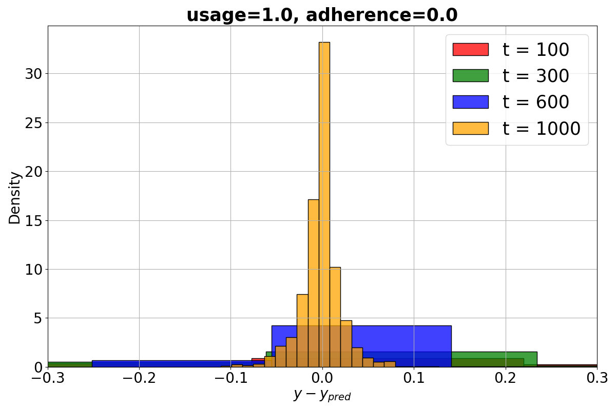
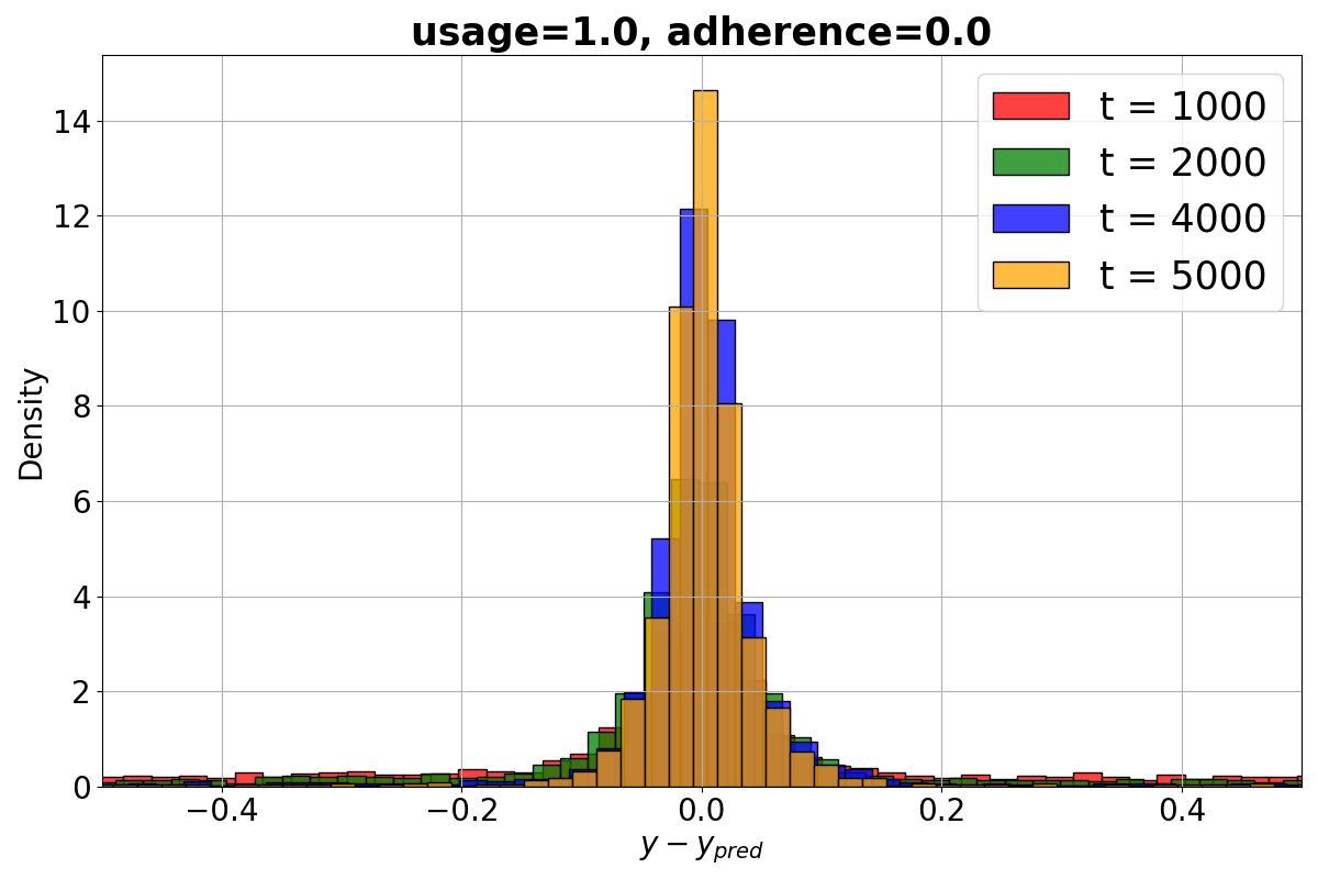
From Fig. 13 we may conclude that is a mixture of the two probability distributions in the current set.