Towards a Scalable Identification of Novel Modes
in Generative Models

Abstract

An interpretable comparison of generative models requires the identification of sample types produced more frequently by each of the involved models. While several quantitative scores have been proposed in the literature to rank different generative models, such score-based evaluations do not reveal the nuanced differences between the generative models in capturing various sample types. In this work, we propose a method called Fourier-based Identification of Novel Clusters (FINC) to identify modes produced by a generative model with a higher frequency in comparison to a reference distribution. FINC provides a scalable stochastic algorithm based on random Fourier features to estimate the eigenspace of kernel covariance matrices of two generative models and utilize the principal eigendirections to detect the sample types present more dominantly in each model. We demonstrate the application of the FINC method to standard computer vision datasets and generative model frameworks. Our numerical results suggest the scalability and efficiency of the developed Fourier-based method in highlighting the sample types captured with different frequencies by widely-used generative models.

1 Introduction

Deep generative models have attained astonishing results on various computer vision datasets. The remarkable quality of image samples produced by state-of-the-art generative models renders manual ranking of these models infeasible. Therefore, to properly compare different generative models and rank their performance, several quantitative scores have been proposed in the computer vision community. Metrics such as Inception Score (IS) [40] and Fréchet Inception Distance (FID) [16] have been widely used in the community for comparing the performance of modern generative model frameworks.

While the standard evaluation scores in the literature offer reliable rankings of generative models, such score-based evaluations do not provide a nuanced comparison between the generative models and how differently they may capture various sample types. However, it is possible that one generative model obtains an inferior score compared to another model, while simultaneously demonstrating higher quality and frequency in producing a limited group of sample types. In such scenarios, a more comprehensive comparison between the generative models highlighting the sample types captured with different frequencies by the models will be useful in revealing their specific strengths and weaknesses. Such a comparison can reveal the suboptimally-generated sample types by each of the compared generative models, which can be used to improve their performance and to further combine them into a unified generative model with the best performance in generating every sample type.

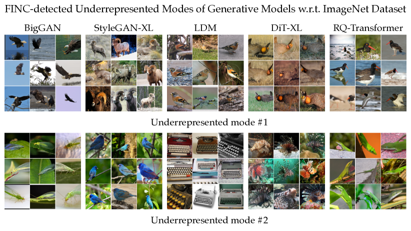
Figure 1: The FINC-identified top two underrepresented modes expressed by test generative models with a considerably lower frequency than in the reference ImageNet dataset.

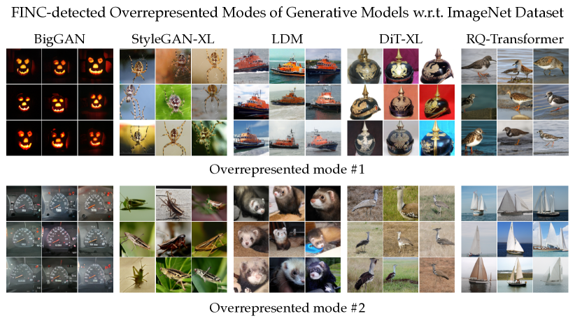
Figure 2: The FINC-identified top two overrepresented modes expressed by test generative models with a considerably higher frequency than in the reference ImageNet dataset.

To achieve the described goal of a detailed comparison between two generative models, we propose to solve a differential clustering problem where we seek to identify the novel sample clusters of a test generative model that are generated significantly more frequently compared to a reference distribution. By addressing the differential clustering task, we can identify the differently-expressed sample types between the two models and perform an interpretable comparison revealing the types of images captured with a higher frequency by each generative model.

To solve the differential clustering problem, one can utilize the scores proposed in the literature to quantify the novelty and uncommonness of generated data. As one such novelty score, [14] proposes the sample-based Rarity score measuring the distance of a generated sample to the manifold of a reference distribution. In another work, [20] formulates Feature Likelihood Divergence (FLD) as a sample-based novelty score based on the sample’s likelihood according to the reference distribution. Note that the application of Rarity and FLD scores to solve the differential clustering task requires a post-clustering of the identified novel samples. Also, [48] suggests the spectral Kernel-based Entropic Novelty (KEN) framework to detect and cluster the novel samples by performing an eigendecomposition of a kernel similarity matrix.

The discussed novelty score-based methods can potentially find the sample types differently captured by two generative models. However, the application of these methods to large-scale datasets containing many sample types, e.g. ImageNet [11], will be computationally challenging. The discussed Rarity and FLD-based methods require a post-clustering of the identified novel samples which will be expensive under a relatively large number of clusters. Furthermore, the KEN method involves the eigendecomposition of a $2n\times 2n$ kernel matrix for a generated data size $n$. However, on the ImageNet dataset with hundreds of image categories, one should perform the analysis on a large sample size $n$ under which performing the eigendecomposition is computationally costly.

In this work, we develop a scalable algorithm, called Fourier-based Identification of Novel Clusters (FINC), to efficiently address the differential clustering problem and find novel sample types of a test generative model compared to another reference model. In the development of FINC, we follow the random Fourier feature framework proposed in [36] and perform the spectral analysis for finding the novel sample types on the covariance matrix characterized by the random Fourier features.

According to the proposed FINC method, we generate a limited number $r$ of random Fourier features to approximate the Gaussian kernel similarity score. We then run a fully stochastic algorithm to estimate the $r\times r$ covariance matrices of the test and reference generative models in the space of selected Fourier features. We prove that applying the spectral decomposition to the resulting $r\times r$ covariance matrix difference will yield the novel clusters of the test model. As a result, the complexity of the algorithm will primarily depend on the Fourier feature size $r$ that can be selected independently of the sample size $n$.

On the theory side, we prove an approximation guarantee that a number $r=\mathcal{O}\bigl{(}\frac{\log n}{\epsilon^{2}}\bigr{)}$ of random features will be sufficient to accurately approximate the principal eigenvalues of the covariance matrices within an $\epsilon$-bounded approximation error and given $n$ samples created by the generative models. As a result, the logarithmic growth of the required Fourier feature size $r$ in the generated data size $n$ shows the scalability of the Fourier-based method for the identification of novel modes between generative models.

We numerically evaluate the performance of our proposed FINC method on large-scale image datasets and generative models. In our numerical analysis, we attempt to identify the novel modes between state-of-the-art generative models to characterize the relative strengths of each generative modeling scheme. Also, we apply FINC to find the suboptimally captured modes of generative models with respect to their target image datasets. For example, Figure 1 shows the FINC-identified underrepresented sample types of five well-known generative models compared to the reference ImageNet dataset used for training the models. These sample types have been generated with a considerably lower frequency compared to the actual ImageNet dataset. On the other hand, Figure 2 shows the FINC-detected overrepresented sample clusters of the same generative models which are produced with a higher frequency compared to the ImageNet dataset. The identification of such clusters could be applied to boost the performance of the models. In the following, we summarize our work’s main contributions:

• Proposing an interpretable comparison approach between generative models using differential clustering,

• Developing the scalable FINC algorithm to identify the differently-expressed sample types by two generative models,

• Providing approximation guarantees on the required number of random Fourier features in the FINC method,

• Presenting the numerical results of applying FINC to compare state-of-the-art image-based generative models.

2 Related Work

Differential Clustering and Random Fourier Features. Several related works [9, 36, 46, 34] explore the application of random Fourier features [36] to clustering and unsupervised learning tasks. Specifically, [9] uses random Fourier features to accelerate kernel clustering by projecting data points into a low-dimension space where the clustering is performed. [46] demonstrates that a Fourier feature-based mapping enhances a neural net’s capability to learn high-frequency functions in low-dimensional data domains. However, the mentioned references do not study the differential clustering problem addressed in our work.

Also, we note that a similar task of differential clustering in the single-cell RNA sequencing domain has been studied in the computational biology literature [29, 2, 33]. Specifically, [2] proposes an algorithm for differential clustering to detect the genes with different expression levels before and after a cell’s condition change. [2]’s method is based on the K-means algorithm and analyzes the norm distances between centers and samples, which would be computationally costly under a large number of clusters. On the other hand, our proposed spectral method can be flexibly combined with random Fourier features to offer a scalable differential clustering method.
Evaluation of generative models. The assessment of deep generative models has been the subject of a large body of related works as surveyed in [5]. The proposed metrics can be categorized into the following groups: 1) distance measures between the generative model and data distribution, including FID [16] and KID [3], 2) scores assessing the quality and diversity of generative models including Inception score [40], precision/recall [39, 25], GAN-train/GAN-test [42], density/coverage [31], Vendi [12], and RKE [19] scores, 3) measures for the train-to-test generalization evaluation of GANs [20, 1, 30].

More specifically, [12, 19] utilize the eigenspectrum of a kernel matrix to quantify diversity. However, unlike our work, these works do not aim for a nuanced sample type-based comparison of generative models. As for the generalizability evaluation, the mentioned references compare a likelihood [20, 1] or distance [30] measure of the generated data between the training and test datasets. We note that the distribution-based novel mode identification in our work is different from the sample-based train-to-test generalizability evaluation, since our goal is to identify modes less-expressed by a reference distribution which can be different from the training set of the generative model.
Novelty assessment of generative models. The recent works [14, 20, 48] study the evaluation of novelty of samples and modes produced by generative models. [14] empirically demonstrates that rare samples are distantly located from the reference data manifold, and proposes the rarity score as the distance to the nearest neighbor for quantifying the uncommonness of a sample. [20] measures the mismatch between the likelihoods evaluated for generated samples with respect to the training set and a reference dataset. We remark that [14, 20] offer sample-based novelty scores which needs to be combined with a post-clustering step to address our target differential clustering task. However, the post-clustering step would be computationally costly under a significant number of clusters. Also, [48] proposes a spectral method for measuring the entropy of the novel modes of a generative model with respect to a reference model, which reduces to the eigendecomposition of a kernel similarity matrix. Consequently, [48]’s algorithm leads to an $\mathcal{O}(n^{3})$ computational complexity given $n$ generated samples, hindering the method’s application to large-scale datasets. In our work, we aim to leverage random Fourier features to reduce the spectral approach’s computational complexity and to provide a scalable solution to the differential clustering task.

3 Preliminaries

3.1 Generative Models and Their Evaluation

Consider a generative model $G$ generating samples from a probability distribution $P_{G}$. Note that the generative model $G$ could represent a function $G:\mathbb{R}^{s}\rightarrow\mathbb{R}^{d}$ mapping a latent $s$-dimensional random vector $\mathbf{Z}\in\mathbb{R}^{s}$ drawn from a known distribution $P_{Z}$ to generated sample $G(\mathbf{Z})\in\mathbb{R}^{d}$ possessing a distribution of interest. The function-based sample production is the mechanism in the well-known frameworks of variational autoencoders (VAEs) [23] and generative adversarial networks (GANs) [13].

On the other hand, in the framework of denoising diffusion probabilistic models (DDPM) [17], the generative model creates data through a randomized iterative process where a noise input is denoised to a limited degree followed by adding a bounded-variance noise vector at every iteration. While this process does not lead to a deterministic generator map, it still leads to the generation of samples from a generative distribution which we denote by $P_{G}$ in our discussion.

Given a generative model $G$ generating samples from $P_{G}$, the goal of a quantitative evaluation is to use a group of $n$ generated data $\mathbf{x}_{1},\ldots,\mathbf{x}_{n}\sim P_{G}$ to compute a score quantifying a desired property of the generated data such as visual quality, diversity, generalizability, and novelty. Note that in such a sample-based evaluation, we do not have access to the cumulative distribution function (CDF) of $P_{G}$ and only observe a group of $n$ samples generated by the model. As discussed in Section 2, multiple scores have been proposed in the literature to assess different properties of generative models.

3.2 Kernel Function and Kernel Covariance Matrix

Consider a kernel function $k:\mathbb{R}^{d}\times\mathbb{R}^{d}\rightarrow\mathbb{R}$ assigning the similarity score $k(\mathbf{x},\mathbf{x}^{\prime})$ to data vectors $\mathbf{x},\mathbf{x}^{\prime}\in\mathbb{R}^{d}$. The kernel function is assumed to satisfy the positive-semidefinite (PSD) property requiring that for every integer $n\in\mathbb{N}$ and vectors $\mathbf{x}_{1},\ldots,\mathbf{x}_{n}\in\mathbb{R}^{d}$, the $n\times n$ kernel matrix $K=\bigl{[}k(\mathbf{x}_{i},\mathbf{x}_{j})\bigr{]}_{n\times n}$ is a PSD matrix. Throughout this paper, we commonly use the Gaussian kernel $k_{\text{\rm Gaussian}(\sigma^{2})}$ which for a bandwidth parameter $\sigma^{2}$ is defined as:

$$k_{\text{\rm Gaussian}(\sigma^{2})}\bigl{(}\mathbf{x},\mathbf{x}^{\prime}\bigr{)}\,:=\,\exp\Bigl{(}\frac{-\|\mathbf{x}-\mathbf{x}^{\prime}\|^{2}_{2}}{2\sigma^{2}}\Bigr{)}$$ (1)

We note that for every kernel function $k$, there exists a feature map $\phi:\mathbb{R}^{d}\rightarrow\mathbb{R}^{s}$ such that $k(\mathbf{x},\mathbf{x}^{\prime})=\phi(\mathbf{x})^{\top}\phi(\mathbf{x}^{\prime})$ is the inner product of $\phi$-based transformations of inputs $\mathbf{x}$ and $\mathbf{x}^{\prime}$. Given the feature map $\phi$ corresponding to kernel $k$, we define the empirical kernel covariance matrix $\widehat{C}_{X}\in\mathbb{R}^{s\times s}$ as

$$\widehat{C}_{X}\,:=\,\frac{1}{n}\sum_{i=1}^{n}\phi\bigl{(}\mathbf{x}_{i}\bigr{)}\phi\bigl{(}\mathbf{x}_{i}\bigr{)}^{\top}$$ (2)

It can be seen that the kernel covariance matrix $\widehat{C}_{X}$ shares the same eigenvalues with the normalized kernel matrix $\frac{1}{n}K=\frac{1}{n}\bigl{[}k(\mathbf{x}_{i},\mathbf{x}_{j})\bigr{]}_{n\times n}$. Assuming a normalized kernel satisfying $k(\mathbf{x},\mathbf{x})=1$ for every $\mathbf{x}\in\mathbb{R}^{d}$, a condition that holds for the Gaussian kernel in (1), the eigenvalues of $\widehat{C}_{X}$ will satisfy the probability axioms and result in a probability model. The resulting probability model, as theoretically shown in [48], will estimate the frequencies of the major modes of a multi-modal distribution with well-separable modes.

3.3 Shift-Invariant Kernels and Random Fourier Features

A kernel function $k:\mathbb{R}^{d}\times\mathbb{R}^{d}\rightarrow\mathbb{R}$ is called shift-invariant if there exists a function $\kappa:\mathbb{R}^{d}\rightarrow\mathbb{R}$ such that for every $\mathbf{x},\mathbf{x}^{\prime}\in\mathbb{R}^{d}$ we have

$$k\bigl{(}\mathbf{x},\mathbf{x}^{\prime}\bigr{)}\,=\,\kappa\bigl{(}\mathbf{x}-\mathbf{x}^{\prime}\bigr{)}$$

In other words, the output of a shift-invariant kernel $k(\mathbf{x},\mathbf{x}^{\prime})$ only depends on the difference $\mathbf{x}-\mathbf{x}^{\prime}$. For example, the Gaussian kernel in (1) represents a shift-invariant kernel. Bochner’s theorem [4] proves that a function $\kappa:\mathbb{R}^{d}\rightarrow\mathbb{R}$ results in a shift-invariant normalized kernel $k(\mathbf{x},\mathbf{x}^{\prime})=\kappa(\mathbf{x}-\mathbf{x}^{\prime})$ if and only if the Fourier transform of $\kappa$ is a probability density function (PDF) taking non-negative values and integrating to $1$. Recall that the Fourier transform of $\kappa:\mathbb{R}^{d}\rightarrow\mathbb{R}$, which we denote by $\widehat{\kappa}:\mathbb{R}^{d}\rightarrow\mathbb{R}$, is defined as

$$\widehat{\kappa}(\boldsymbol{\omega})\,:=\,\int\kappa(\mathbf{x})\exp\bigl{(}-i\boldsymbol{\omega}^{\top}\mathbf{x}\bigr{)}\mathrm{d}\mathbf{x}$$

For example, in the case of Gaussian kernel (1) with bandwidth parameter $\sigma^{2}$, the Fourier transform will be the PDF of Gaussian distribution $\mathcal{N}(\mathbf{0},\frac{1}{\sigma^{2}}I_{d})$ with zero mean vector and isotropic covaraince matrix $\frac{1}{\sigma^{2}}I_{d}$. Based on Bochner’s theorem, [36, 37, 44] suggest using $r$ random Fourier features $\boldsymbol{\omega}_{1},\ldots,\boldsymbol{\omega}_{r}\sim\widehat{\kappa}$ drawn independently from PDF $\widehat{\kappa}$, and approximating the shift-invariant kernel function $\kappa(\mathbf{x}-\mathbf{x}^{\prime})$ as follows where $\phi_{r}(\mathbf{x})=\frac{1}{\sqrt{r}}\bigl{[}\cos(\boldsymbol{\omega}_{1}^{\top}\mathbf{x}),\sin(\boldsymbol{\omega}_{1}^{\top}\mathbf{x}),\ldots,\cos(\boldsymbol{\omega}_{r}^{\top}\mathbf{x}),\sin(\boldsymbol{\omega}_{r}^{\top}\mathbf{x})\bigr{]}$ denotes the normalized feature map characterized by the random Fourier features:

$$k\bigl{(}\mathbf{x},\mathbf{x}^{\prime}\bigr{)}\,\approx\,\phi_{r}(\mathbf{x})^{\top}\phi_{r}(\mathbf{x}^{\prime})$$

4 A Scalable Algorithm for the Identification of Novel Sample Clusters between Generative Models

To provide an interpretable comparison between the test generative model $P_{G}$ and the reference distribution $P_{\text{\rm ref}}$, we aim to find the sample clusters generated significantly more frequently by the test model $P_{G}$ compared to the reference model $P_{\text{\rm ref}}$. We suppose we have access to $n$ independent samples $\mathbf{x}_{1},\ldots,\mathbf{x}_{n}$ from $P_{G}$ as well as $m$ independent samples $\mathbf{y}_{1},\ldots,\mathbf{y}_{m}$ from $P_{\text{\rm ref}}$. To address the comparison task, we propose solving a differential clustering problem to find clusters of test samples that have a significantly higher likelihood according to $P_{G}$ than according to $P_{\text{\rm ref}}$.

To address the differential clustering task, we follow the spectral approach proposed in [48], where for a parameter $\rho\geq 1$ we define the $\rho$-conditional kernel covariance matrix $\Lambda_{\mathbf{X}|\rho\mathbf{Y}}$ as the following difference of the kernel covariance matrices $\widehat{C}_{\mathbf{X}},\,\widehat{C}_{\mathbf{Y}}$ of the test and reference data, respectively, as defined in (2):

$$\Lambda_{\mathbf{X}|\rho\mathbf{Y}}\,:=\,\widehat{C}_{\mathbf{X}}-\rho\,\widehat{C}_{\mathbf{Y}}$$ (3)

As proven in [48], under multi-modal distributions $P_{G}$ and $P_{\text{\rm ref}}$ with well-separable modes, the eigenvectors corresponding to the positive eigenvalues of the above matrix will reveal the modes of $\mathbf{X}$ which has a frequency $\rho$-times greater than the mode’s frequency in $\mathbf{Y}$. We remark that the constant $\rho$ can be interpreted as the novelty threshold, which the novelty evaluation requires the detected modes of $P_{G}$ to possess compared to $P_{\text{\rm ref}}$. Therefore, our goal is to find the eigenvectors corresponding to the maximum eigenvalues of the conditional covariance matrix.

The reference [48] applies the kernel trick to solve the problem which leads to the eigendecomposition of an $(m+n)\times(m+n)$ kernel similarity matrix which shares the same eigenvalues with $\Lambda_{\mathbf{X}|\rho\mathbf{Y}}$. However, the resulting eigendecompositon task will be computationally challenging for significantly large $m$ and $n$ sample sizes. Furthermore, while the eigenvectors of [48]’s kernel matrix can cluster the test and reference samples, they do not offer a general clustering rule applicable to fresh samples from $P_{G}$ which would be desired if the learner plans to find the cluster of newly-generated samples from $P_{G}$.

In this work, we propose to leverage the framework of random Fourier features (RFF) [36] to find a scalable solution to the eigendecomposition of $\Lambda_{\mathbf{X}|\rho\mathbf{Y}}$. Unlike [48], we do not utilize the kernel trick and aim to directly apply the spectral decomposition to $\Lambda_{\mathbf{X}|\rho\mathbf{Y}}$. However, under the assumed Gaussian kernel similarity measure, the dimensions of the target $\rho$-conditional kernel covariance matrix is not finite. To resolve this challenge, we approximate the eigenspace of the original $\Lambda_{\mathbf{X}|\rho\mathbf{Y}}$ with that of the covariance matrix of the random Fourier features.

Specifically, assuming a Gaussian kernel $k_{\text{\rm Gaussian}(\sigma^{2})}$ with bandwidth $\sigma^{2}$, we sample $r$ independent vectors $\boldsymbol{\omega}_{1},\ldots,\boldsymbol{\omega}_{r}\sim\mathcal{N}(\mathbf{0},\frac{1}{\sigma^{2}}I_{d})$ from a zero-mean Gaussian distribution with covariance matrix $\frac{1}{\sigma^{2}}I_{d}$ where $I_{d}$ denotes the $d$-dimensional identity matrix. Given the randomly-sampled frequency parameters, we consider the following feature map $\widetilde{\phi}_{r}:\mathbb{R}^{d}\rightarrow\mathbb{R}^{2r}$:

$$\widetilde{\phi}_{r}(\mathbf{x})\,:=\,\frac{1}{\sqrt{r}}\Bigl{[}\cos\bigl{(}\boldsymbol{\omega}_{1}^{\top}\mathbf{x}\bigr{)},\sin\bigl{(}\boldsymbol{\omega}_{1}^{\top}\mathbf{x}\bigr{)},\ldots,\cos\bigl{(}\boldsymbol{\omega}_{r}^{\top}\mathbf{x}\bigr{)},\sin\bigl{(}\boldsymbol{\omega}_{r}^{\top}\mathbf{x}\bigr{)}\Bigr{]}.$$

Then, we compute the positive eigenvalues and corresponding eigenvectors of the following RFF-based $\rho$-conditional kernel covariance matrix ${\widetilde{\Lambda}}_{\mathbf{X}|\rho\mathbf{Y}}\in\mathbb{R}^{2r\times 2r}$:

$${\widetilde{\Lambda}}_{\mathbf{X}|\rho\mathbf{Y}}\,:= \,\widetilde{C}_{\mathbf{X}}-\rho\widetilde{C}_{\mathbf{Y}},$$ (4)

$$\text{\rm where }\quad\;\;\widetilde{C}_{\mathbf{X}}\,:= \,\frac{1}{n}\sum_{i=1}^{n}\widetilde{\phi}_{r}(\mathbf{x}_{i})\widetilde{\phi}_{r}(\mathbf{x}_{i})^{\top},\;\;\widetilde{C}_{\mathbf{Y}}\,:=\,\frac{1}{m}\sum_{j=1}^{m}\widetilde{\phi}_{r}(\mathbf{y}_{j})\widetilde{\phi}_{r}(\mathbf{y}_{j})^{\top}\,.$$

Therefore, instead of the original ${{\Lambda}}_{\mathbf{X}|\rho\mathbf{Y}}$ with an infinite dimension, we only need to run the spectral eigendecomposition algorithm on the $2r\times 2r$ matrix ${\widetilde{\Lambda}}_{\mathbf{X}|\rho\mathbf{Y}}$. Furthermore, the computation of both $\widetilde{C}_{\mathbf{X}}$ and $\widetilde{C}_{\mathbf{Y}}$ can be performed using a stochastic algorithm for averaging the $2r\times 2r$ sample-based matrix $\widetilde{\phi}_{r}(\mathbf{x}_{i})\widetilde{\phi}_{r}(\mathbf{x}_{i})^{\top}$’s and $\widetilde{\phi}_{r}(\mathbf{y}_{j})\widetilde{\phi}_{r}(\mathbf{y}_{j})^{\top}$’s.

Algorithm 1, which we call the Fourier-based Identification of Novel Clusters (FINC), contains the steps explained above to reach a scalable algorithm for approximating the top more-frequently generated modes of $\mathbf{X}\sim P_{G}$ with respect to $\mathbf{Y}\sim P_{\text{\rm ref}}$. The following theorem proves that by choosing $r=\mathcal{O}(\frac{\log(n+m)}{\epsilon^{4}})$, the approximation error of the random Fourier-based method is bounded by $\epsilon$.

Algorithm 1 Fourier-based Identification of Novel Clusters (FINC)

1:Input: Sample sets $\{\mathbf{x}_{1},\ldots,\mathbf{x}_{n}\}$ and $\{\mathbf{y}_{1},\ldots,\mathbf{y}_{m}\}$, Gaussian kernel bandwidth $\sigma^{2}$, parameter $\rho$, feature number $r$

2:Draw $r$ Gaussian random vectors $\boldsymbol{\omega}_{1},\ldots,\boldsymbol{\omega}_{r}\sim\mathcal{N}\bigl{(}\mathbf{0},\frac{1}{\sigma^{2}}I_{d\times d}\bigr{)}$

3:Create the map $\widetilde{\phi}_{r}(\mathbf{x})=\frac{1}{\sqrt{r}}\bigl{[}\cos(\boldsymbol{\omega}_{1}^{\top}\mathbf{x}),\sin(\boldsymbol{\omega}_{1}^{\top}\mathbf{x}),\ldots,\cos(\boldsymbol{\omega}_{r}^{\top}\mathbf{x}),\sin(\boldsymbol{\omega}_{r}^{\top}\mathbf{x})\bigr{]}$

4:Initialize $\widetilde{C}_{X},\widetilde{C}_{Y}=\mathbf{0}_{r\times r}$

5:for $i\in\bigl{\{}1,\ldots,\max\{n,m\}\bigr{\}}$  do

6:     Update $\widetilde{C}_{X}\leftarrow\widetilde{C}_{X}+\frac{1}{n}{\widetilde{\phi}}_{r}(\mathbf{x}_{i}){\widetilde{\phi}}_{r}(\mathbf{x}_{i})^{\top}$

7:     Update $\widetilde{C}_{Y}\leftarrow\widetilde{C}_{Y}+\frac{1}{m}{\widetilde{\phi}}_{r}(\mathbf{y}_{i}){\widetilde{\phi}}_{r}(\mathbf{y}_{i})^{\top}$

8:end for

9:Compute $\widetilde{\Lambda}_{\mathbf{X}|\mathbf{Y}}=\widetilde{C}_{X}-\rho\widetilde{C}_{Y}$

10:Apply spectral eigendecomposition to obtain $\widetilde{\Lambda}_{\mathbf{X}|\mathbf{Y}}=U^{\top}\mathrm{diag}(\boldsymbol{\lambda})U$

11:Find the positive eigenvalues $\lambda_{1},\ldots,\lambda_{t}>0$

12:Output: Eigenvalues $\lambda_{1},\ldots,\lambda_{t}$ and eigenvectors $\mathbf{u}_{1},\ldots,\mathbf{u}_{t}$.

Theorem 1.

Suppose $\boldsymbol{\omega}_{1},\ldots,\boldsymbol{\omega}_{r}$ are independently drawn from the Gaussian distribution $\mathcal{N}(\mathbf{0},\sigma^{-2}I_{d})$ and define $r^{\prime}=\min\{2r,m+n\}$. Let ${\widetilde{\lambda}}_{1}\geq\cdots\geq{\widetilde{\lambda}}_{r^{\prime}}$ be the sorted top-$r^{\prime}$ eigenvalues of ${\widetilde{\Lambda}}_{\mathbf{X}|\rho\mathbf{Y}}$ with corresponding eigenvectors ${\widetilde{\mathbf{v}}}_{1},\ldots,{\widetilde{\mathbf{v}}}_{r^{\prime}}$. Similarly, define ${{\lambda}}_{1}\geq\cdots\geq{{\lambda}}_{r^{\prime}}$ as the sorted top-$r^{\prime}$ eigenvalues of ${{\Lambda}}_{\mathbf{X}|\rho\mathbf{Y}}$. Then, for every $\delta>0$, with probability at least $1-\delta$ we will have the following approximation guarantee with $\epsilon=\bigl{(}2(1+\rho)\bigr{)}^{3/2}\sqrt[4]{\frac{\log((m+n)/{\delta})}{r}}$:

$$\sqrt{\sum_{i=1}^{r^{\prime}}\bigl{(}{\widetilde{\lambda}}_{i}-{\lambda}_{i}\bigr{)}^{2}}\,\leq\,\epsilon\quad\text{\rm and}\quad\max_{1\leq i\leq r^{\prime}}\,\Bigl{\|}{\Lambda}_{\mathbf{X}|\rho\mathbf{Y}}\mathbf{v}_{i}-{\lambda}_{i}\mathbf{v}_{i}\Bigr{\|}_{2}\,\leq\,2(1+\rho)\epsilon,$$

where for every $i$ we define $\mathbf{v}_{i}=\sum_{t=1}^{n}\bigl{(}\widetilde{\mathbf{v}}^{\top}_{i}\widetilde{\phi}_{r}(\mathbf{x}_{i})\bigr{)}\phi(\mathbf{x}_{i})+\sum_{s=1}^{m}\bigl{(}\widetilde{\mathbf{v}}^{\top}_{i}\widetilde{\phi}_{r}(\mathbf{y}_{s})\bigr{)}\phi(\mathbf{y}_{s})$ as the proxy eigenvector corresponding to the given $\widetilde{\mathbf{v}}_{i}$.

Proof.

We relegate the proof to the Appendix. ∎

Theorem 1 proves that the eigenvalues and eigenvectors of the Fourier-based approximation $\widetilde{\Lambda}_{\mathbf{X}|\rho\mathbf{Y}}$ will be $\epsilon$-close to those of the original conditional kernel covariance matrix ${\Lambda}_{\mathbf{X}|\rho\mathbf{Y}}$, conditioned that we have $r=\mathcal{O}(\frac{\log(m+n)}{\epsilon^{4}})$ number of random Fourier features. Therefore, for a fixed $\epsilon$ value, the required number of random Fourier features grows only logarithmically with the test and reference sample size $m+n$. This guarantee shows that the computational complexity of FINC could be significantly less than the kernel-based approach in [48] applying an eigendecomposition to an $(m+n)\times(m+n)$ kernel matrix.

5 Numerical Evaluation

5.1 Experimental Setting

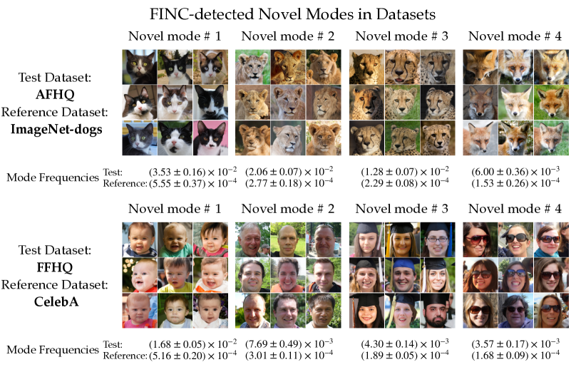
Figure 3: FINC-identified top novel modes between datasets. Detected novel modes have at least 10 times higher frequency in the test datasets than the reference case.

Datasets. We performed the numerical experiments on the following standard image datasets: 1) ImageNet-1K [11] containing 1.4 million images with 1000 labels. The ImageNet-dogs subset used in our experiments includes 20k dog images from 120 different breeds, 2) CelebA [28] containing 200k human face images from celebrities, 3) FFHQ [22] including 70k human-face images, 4) AFHQ [10] including 15k dogs, cats, and wildlife animal-face images.
Tested generative models and feature extraction: Following the standard in the literature of generative model evaluation, we utilized an Inception-V3 neural network [45] pre-trained on ImageNet to perform feature extraction. The extracted feature vector was 2048-dimensional. Also, we downloaded the pre-trained generative models from DINOv2 [43] repository.
Hyper-parameters selection and sample size: Similar to the kernel-based evaluation in [19], we chose the kernel bandwidth $\sigma^{2}$ by searching for the smallest $\sigma$ value resulting in a variance bounded by $0.01$. Also, we conducted the experiments using at least $m,n=50$k sample sizes for the test and reference generative models, with the exception of dataset AFHQ and ImageNet-dogs, where the dataset’s size was smaller than $50$k. For these datasets, we used the entire dataset in the differential clustering. For Fourier feature size $r$, we tested $r$ values in $\{500,1000,2000,4000\}$ to find the size obtaining an approximation error estimate below 1%, and $r=2000$ consistently fulfilled the goal in the experiments.

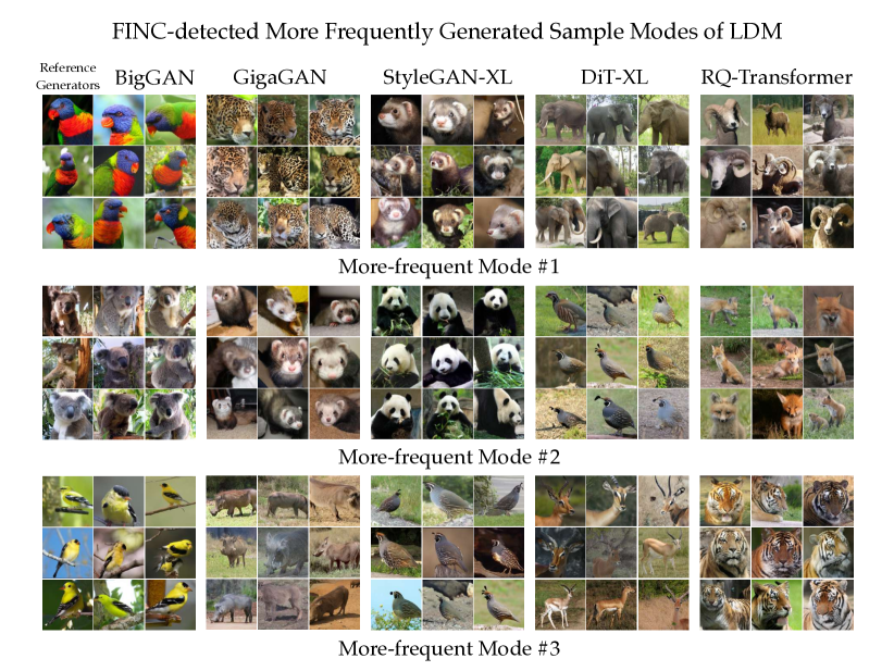
Figure 4: Representative samples from FINC-detected top-3 modes with the maximum frequency gap between LDM (higher frequency) and reference generative models.

5.2 Identification of More-Frequent and Novel Modes via FINC

We evaluated the performance of FINC in detecting novel modes of the test model with a frequency $\rho$-times greater than that under the reference mode using the novelty threshold $\rho=10$. First, we performed a sanity check of the proposed FINC method in detecting novel modes between real dataset pairs, where our knowledge of the nature of the dataset could be informative about the novel modes. For example, the novel modes of the AFHQ dataset compared to ImageNet-dogs are expected to contain cats and wildlife, and the novel modes of the FFHQ dataset compared to the CelebA dataset could relate to traits appearing less frequently among celebrities, e.g. a below-$10$ age. Figure 3 shows FINC-detected top-4 novel modes for AFHQ/ImageNet-dogs and FFHQ/CelebA, which look consistent with our expected novel types based on the datasets’ structure.

Next, we applied FINC to detect novel modes between various generative models trained on ImageNet-1K and FFHQ. We tested generative models following standard frameworks, including GAN-based BigGAN [6], GigaGAN [21], StyleGAN-XL [41], InsGen [47], diffusion-based LDM [38], DiT-XL [32], and VAE-based RQ-Transformer [26], VDVAE [8]. Figure 4 displays FINC-detected more frequently generated modes of LDM compared to the reference models with threshold $\rho=1$. Next, we reversed the role of test and reference generators to detect less frequently generated modes of LDM in Figure 5. These figures suggest that the LDM model reached relatively higher frequencies for several terrestrial animals, while it led to lower frequencies in sample types such as mushrooms and birds. Subsequently, we considered a higher novelty threshold $\rho=5$. Figure 6 shows the FINC-detected novel modes in StyleGAN-XL containing sample types such as ”painted portrait” and ”child with a round hat”.

Also, we used the eigenfunctions corresponding to the computed eigenvectors to assign a mode-based similarity score to fresh unseen images. As Theorem 1 implies, the mode-scoring function for the eigenvector $\widetilde{\mathbf{v}}$ is $s_{\tilde{\mathbf{v}}}(\mathbf{x})=\sum_{i=1}^{r}{\tilde{v}}_{2i-1}\cos({\boldsymbol{\omega}}_{i}^{\top}\mathbf{x})+{\tilde{v}}_{2i}\sin({\boldsymbol{\omega}}_{i}^{\top}\mathbf{x})$. This likelihood quantification can apply to both train data and fresh unseen data not contained in the sample sets for running FINC. Figure 7 displays the evaluated scores under two pairs of datasets, where we measured and ranked a group of unseen data according to the FINC-detected modes’ scoring function. The FINC-based assigned scores indicate a semantically meaningful ranking of the images’ likelihood of belonging to the displayed modes.

Figure 5: Representative samples from FINC-detected top-3 modes with the maximum frequency gap between LDM (lower frequency) and reference generative models.

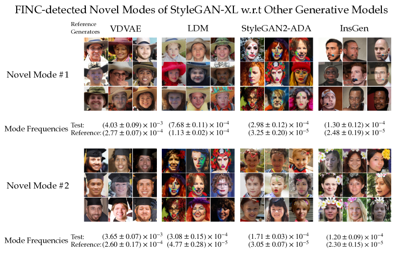
Figure 6: Representative samples from FINC-detected top-3 novel modes (novelty threshold $\rho=5$) of StyleGAN-XL compared to reference generative models.

5.3 Scalability of FINC in the Identification of Novel Modes

Scalability is a key property of a differential clustering algorithm in application to a data distribution with a significant number of modes, such as ImageNet-1K. To evaluate the scalability of the proposed FINC method compared to the baselines, we recorded the time (in seconds) of running the algorithm on the ImageNet-based experiments in Figures 1 and 2. For baselines, we downloaded the implementation of the Rarity score [14], FLD score [20], and KEN method [48], and measured their time for detecting the novel samples followed by a spectral-clustering step performed by the standard TorchCluster package.

Table 1 shows the time taken by FINC with $r=2000$ and the baselines on different sample sizes (we suppose $n=m$), suggesting an almost linearly growing time with sample size in the case of FINC. In contrast, the baselines’ spent time grew at a superlinear rate, and for sample sizes larger than 10k and 50k all the baselines ran into a memory overflow on the GPU and CPU processors.

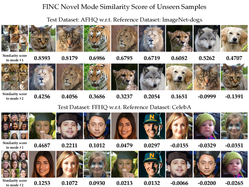
Figure 7: Computing FINC-assigned mode score for 8 unseen samples and 2 detected modes. Images looking more similar to the modes are supposed to have higher scores. (Top-half) AFHQ w.r.t. ImageNet-dogs, (Bottom-half) FFHQ w.r.t. CelebA.

Table 1: Time complexity (in seconds) of solving the differential clustering problem on the ImageNet dataset using the proposed FINC method vs. the baselines. The dash - means failure due to memory overflow, and $>24h$ implies not complete in 24 hours.

		Sample Size
Processor	Method	1k	2.5k	5k	10k	25k	50k	100k	250k
	Rarity+spectral clustering [14]	1.4	9.1	37.6	153.5	1030	4616	-	-
	FLD+spectral clustering [20]	2.7	14.3	59.4	224.5	1408	6024	-	-
	KEN+eigen-decomposition[48]	3.5	26.3	122.8	1130	14354	$>$24h	-	-
	KEN+Cholesky-decomposition[48]	2.6	16.1	61.7	266.0	2045	10934	-	-
CPU	FINC ($r=2000$)	13.1	31.6	62.8	125.5	311.2	617.6	1248	3090
	Rarity+spectral clustering [14]	0.1	4.3	10.7	27.6	-	-	-	-
	FLD+spectral clustering [20]	0.2	3.7	10.8	25.1	-	-	-	-
	KEN+eigen-decomposition[48]	1.1	11.6	52.1	455.6	-	-	-	-
	KEN+Cholesky-decomposition[48]	0.1	0.7	3.2	16.7	-	-	-	-
GPU	FINC ($r=2000$)	0.5	1.0	1.6	3.1	7.6	15.0	29.8	74.3

6 Conclusion

In this work, we developed a scalable algorithm to find the differently-expressed modes of two generative models. The proposed Fourier-based approach attempts to solve a differential clustering problem to find the sample clusters generated with significantly different frequencies by the test generative model and a reference distribution. We demonstrated the application of the proposed methodology in finding the suboptimally captured modes in a generative model compared to a reference distribution. An interesting future direction to this work is to extend the comparison framework to more than two generative models, where instead of a pairwise comparison, one can simultaneously compare the modes generated by multiple generative models. Also, a potential application of the method for future studies is to boost the performance of multiple generative models using a proper combination characterized by their FINC-based comparison.

Appendix A Proofs

A.1 Proof of Theorem 1

First, note that the Gaussian probability density function (PDF) $\mathcal{N}\bigl{(}\mathbf{0},\sigma^{-2}I_{d}\bigr{)}$ is proportional to the Fourier transform of the Gaussian kernel in (1), because for the corresponding shift-invariant kernel producing function $\kappa_{\sigma}(\mathbf{x})=\exp\bigl{(}\frac{-\|\mathbf{x}\|^{2}_{2}}{2\sigma^{2}}\bigr{)}$ we have the following Fourier transform:

$$\widehat{\kappa_{\sigma}}(\boldsymbol{\omega})\, =\,\int\kappa_{\sigma}(\mathbf{x})\exp(-i\boldsymbol{\omega}^{\top}\mathbf{x})\mathrm{d}\mathbf{x}$$

$$=\,\Bigl{(}{2\pi}{\sigma^{2}}\Bigr{)}^{d/2}\exp\Bigl{(}-\frac{\sigma^{2}\|\boldsymbol{\omega}\|^{2}_{2}}{2}\Bigr{)}$$

$$=\,(2\pi)^{d}\underbrace{\Bigl{(}\frac{1}{2\pi\sigma^{-2}}\Bigr{)}^{d/2}\exp\Bigl{(}-\frac{\|\boldsymbol{\omega}\|^{2}_{2}}{2\sigma^{-2}}\Bigr{)}}_{\text{\rm PDF of}\;\,\mathcal{N}(\mathbf{0},\sigma^{-2}I)}.$$

On the other hand, according to the synthesis property of Fourier transform we can write

$$k_{\text{\rm Gaussian}(\sigma^{2})}\bigl{(}\mathbf{x},\mathbf{x}^{\prime}\bigr{)}\, =\,\kappa_{\sigma}\bigl{(}\mathbf{x}-\mathbf{x}^{\prime}\bigr{)}$$

$$\stackrel{{\scriptstyle(a)}}{{=}}\,\frac{1}{(2\pi)^{d}}\int\widehat{\kappa_{\sigma}}(\boldsymbol{\omega})\exp\bigl{(}i\boldsymbol{\omega}^{\top}(\mathbf{x}-\mathbf{x}^{\prime})\bigr{)}\mathrm{d}\boldsymbol{\omega}$$

$$\stackrel{{\scriptstyle(b)}}{{=}}\,\int\frac{1}{(2\pi)^{d}}\widehat{\kappa_{\sigma}}(\boldsymbol{\omega})\cos\bigl{(}\boldsymbol{\omega}^{\top}(\mathbf{x}-\mathbf{x}^{\prime})\bigr{)}\mathrm{d}\boldsymbol{\omega}$$

$$\stackrel{{\scriptstyle(c)}}{{=}}\,\mathbb{E}_{\boldsymbol{\omega}\sim\mathcal{N}(\mathbf{0},\sigma^{-2}I)}\Bigl{[}\cos\bigl{(}\boldsymbol{\omega}^{\top}(\mathbf{x}-\mathbf{x}^{\prime})\bigr{)}\Bigr{]}$$

$$=\,\mathbb{E}_{\boldsymbol{\omega}\sim\mathcal{N}(\mathbf{0},\sigma^{-2}I)}\Bigl{[}\cos\bigl{(}\boldsymbol{\omega}^{\top}\mathbf{x})\cos\bigl{(}\boldsymbol{\omega}^{\top}\mathbf{x}^{\prime})+\sin\bigl{(}\boldsymbol{\omega}^{\top}\mathbf{x})\sin\bigl{(}\boldsymbol{\omega}^{\top}\mathbf{x}^{\prime})\Bigr{]}$$

In the above, (a) follows from the synthesis equation of Fourier transform. (b) uses the fact that $\widehat{\kappa_{\sigma}}$ is an even function, leading to a zero imaginary term in the Fourier synthesis equation. (c) use the relationship between $\widehat{\kappa_{\sigma}}$ and the PDF of $\mathcal{N}(\mathbf{0},\sigma^{-2}I)$. Therefore, since $\bigl{|}\cos\bigl{(}\boldsymbol{\omega}^{\top}\mathbf{y}\bigr{)}\bigr{|}\leq 1$ holds for every $\boldsymbol{\omega}$ and $\mathbf{y}$, we can apply Hoeffding’s inequality to show that for independently sampled $\boldsymbol{\omega}_{1},\ldots,\boldsymbol{\omega}_{r}\stackrel{{\scriptstyle\mathrm{iid}}}{{\sim}}\mathcal{N}(\mathbf{0},\sigma^{-2}I)$ the following probabilistic bound holds:

$$\mathbb{P}\biggl{(}\Bigl{|}\frac{1}{r}\sum_{i=1}^{r}\cos\bigl{(}\boldsymbol{\omega}_{i}^{\top}(\mathbf{x}-\mathbf{x}^{\prime})\bigr{)}-\mathbb{E}_{\boldsymbol{\omega}\sim\mathcal{N}(\mathbf{0},\sigma^{-2}I)}\Bigl{[}\cos\bigl{(}\boldsymbol{\omega}^{\top}(\mathbf{x}-\mathbf{x}^{\prime})\bigr{)}\Bigr{]}\Bigr{|}\geq\epsilon\biggr{)}\leq 2\exp\Bigl{(}-\frac{r\epsilon^{2}}{2}\Bigr{)}$$

However, note that the identity $\cos(a-b)=\cos(a)\cos(b)+\sin(a)\sin(b)$ implies that $\frac{1}{r}\sum_{i=1}^{r}\cos\bigl{(}\boldsymbol{\omega}_{i}^{\top}(\mathbf{x}-\mathbf{x}^{\prime})\bigr{)}\,=\,\widetilde{\phi}_{r}(\mathbf{x})^{\top}\widetilde{\phi}_{r}(\mathbf{x}^{\prime})$ and so we can rewrite the above bound as

$$\mathbb{P}\biggl{(}\Bigl{|}\widetilde{\phi}_{r}(\mathbf{x})^{\top}\widetilde{\phi}_{r}(\mathbf{x}^{\prime})-k_{\text{\rm Gaussian}(\sigma^{2})}(\mathbf{x},\mathbf{x}^{\prime})\Bigr{|}\geq\epsilon\biggr{)}\leq 2\exp\Bigl{(}-\frac{r\epsilon^{2}}{2}\Bigr{)}.$$

Note that both $k_{\text{\rm Gaussian}(\sigma^{2})}$ and $\widetilde{k}_{r}(\mathbf{x},\mathbf{x}^{\prime})=\widetilde{\phi}_{r}(\mathbf{x})^{\top}\widetilde{\phi}_{r}(\mathbf{x}^{\prime})$ are normalized kernels, implying that

$$\forall\mathbf{x}\in\mathbb{R}^{d}:\quad\widetilde{\phi}_{r}(\mathbf{x})^{\top}\widetilde{\phi}_{r}(\mathbf{x})-k_{\text{\rm Gaussian}(\sigma^{2})}(\mathbf{x},\mathbf{x})\,=\,0.$$

In addition, the application of the union bound shows that over the test sample set $\mathbf{x}_{1},\ldots,\mathbf{x}_{n}$, we can write

$$\mathbb{P}\biggl{(}\max_{1\leq i,j\leq n}\Bigl{(}\widetilde{\phi}_{r}(\mathbf{x}_{i})^{\top}\widetilde{\phi}_{r}(\mathbf{x}_{j})-k_{\text{\rm Gaussian}(\sigma^{2})}(\mathbf{x}_{i},\mathbf{x}_{j})\Bigr{)}^{2}\geq\epsilon^{2}\biggr{)}\leq 2{n\choose 2}\exp\Bigl{(}-\frac{r\epsilon^{2}}{2}\Bigr{)}.$$

Similarly, we can show the following concerning the reference sample set $\{\mathbf{y}_{1},\ldots,\mathbf{y}_{m}\}$

$$\mathbb{P}\biggl{(}\max_{1\leq i\leq n,\,1\leq j\leq m}\Bigl{(}\widetilde{\phi}_{r}(\mathbf{x}_{i})^{\top}\widetilde{\phi}_{r}(\mathbf{y}_{j})-k_{\text{\rm Gaussian}(\sigma^{2})}(\mathbf{x}_{i},\mathbf{y}_{j})\Bigr{)}^{2}\geq\epsilon^{2}\biggr{)}\leq 2mn\exp\Bigl{(}-\frac{r\epsilon^{2}}{2}\Bigr{)},$$

$$\mathbb{P}\biggl{(}\max_{1\leq i,j\leq m}\Bigl{(}\widetilde{\phi}_{r}(\mathbf{y}_{i})^{\top}\widetilde{\phi}_{r}(\mathbf{y}_{j})-k_{\text{\rm Gaussian}(\sigma^{2})}(\mathbf{y}_{i},\mathbf{y}_{j})\Bigr{)}^{2}\geq\epsilon^{2}\biggr{)}\leq 2{m\choose 2}\exp\Bigl{(}-\frac{r\epsilon^{2}}{2}\Bigr{)}$$

Applying the union bound, we can utilize the above inequalities to show

$$\mathbb{P}\biggl{(} \max_{1\leq i,j\leq n}\Bigl{(}\widetilde{\phi}_{r}(\mathbf{x}_{i})^{\top}\widetilde{\phi}_{r}(\mathbf{x}_{j})-k_{\text{\rm Gaussian}(\sigma^{2})}(\mathbf{x}_{i},\mathbf{x}_{j})\Bigr{)}^{2}\geq\epsilon^{2}$$

OR $$\max_{1\leq i,j\leq m}\Bigl{(}\widetilde{\phi}_{r}(\mathbf{y}_{i})^{\top}\widetilde{\phi}_{r}(\mathbf{y}_{j})-k_{\text{\rm Gaussian}(\sigma^{2})}(\mathbf{y}_{i},\mathbf{y}_{j})\Bigr{)}^{2}\geq\epsilon^{2}$$

OR $$\max_{1\leq i\leq n,\,1\leq j\leq m}\Bigl{(}\widetilde{\phi}_{r}(\mathbf{x}_{i})^{\top}\widetilde{\phi}_{r}(\mathbf{y}_{j})-k_{\text{\rm Gaussian}(\sigma^{2})}(\mathbf{x}_{i},\mathbf{y}_{j})\Bigr{)}^{2}\geq\epsilon^{2}\biggr{)}$$

$$\leq\; \Bigl{(}2{m\choose 2}+2{n\choose 2}+2mn\Bigr{)}\exp\Bigl{(}-\frac{r\epsilon^{2}}{2}\Bigr{)}$$

$$<\; (m+n)^{2}\exp\Bigl{(}-\frac{r\epsilon^{2}}{2}\Bigr{)}$$ (5)

On the other hand, according to Theorem 3 from [48], we know that the non-zero eigenvalues of the $\rho$-conditional covariance matrix $\Lambda_{\mathbf{X}|\rho\mathbf{Y}}:=\widehat{C}_{\mathbf{X}}-\rho\widehat{C}_{\mathbf{Y}}$ are shared with the $\rho$-conditional kernel matrix

$$K_{\mathbf{X}|\rho\mathbf{Y}}:=\begin{bmatrix}\frac{1}{n}K_{XX}&\sqrt{\frac{\rho}{mn}}K_{XY}\vspace{2mm}\\ -\sqrt{\frac{\rho}{mn}}K^{\top}_{XY}&\frac{-\rho}{m}K_{YY}\end{bmatrix}$$

where the kernel function is the Gaussian kernel $k_{\text{\rm Gaussian}(\sigma^{2})}$. Then, defining the diagonal matrix $D=\mathrm{diag}\bigl{(}[\underbrace{1,\ldots,1}_{n\,\text{\rm times}},\underbrace{-1,\ldots,-1}_{m\,\text{\rm times}}]\bigr{)}$, we observe that

$$K_{\mathbf{X}|\rho\mathbf{Y}}\,=\,D\cdot\underbrace{\begin{bmatrix}\frac{1}{n}K_{XX}&\sqrt{\frac{\rho}{mn}}K_{XY}\vspace{2mm}\\ \sqrt{\frac{\rho}{mn}}K^{\top}_{XY}&\frac{\rho}{m}K_{YY}\end{bmatrix}}_{K_{\mathbf{X,\rho\mathbf{Y}}}}$$

where we define $K_{\mathbf{X,\rho\mathbf{Y}}}$ as the joint kernel matrix that is guaranteed to be a symmetric PSD matrix. Therefore, there exists a unique symmetric and PSD matrix $\sqrt{K_{\mathbf{X,\rho\mathbf{Y}}}}$ which is the square root of $K_{\mathbf{X,\rho\mathbf{Y}}}$. Since for every matrices $A,\,B$ where $AB$ and $BA$ are well-defined, $AB$ and $BA$ share the same non-zero eigenvalues, we conclude that $K_{\mathbf{X}|\rho\mathbf{Y}}\,=\,DK_{\mathbf{X,\rho\mathbf{Y}}}$ has the same non-zero eigenvalues as $\underline{K}=\sqrt{K_{\mathbf{X,\rho\mathbf{Y}}}}\,D\,\sqrt{K_{\mathbf{X,\rho\mathbf{Y}}}}$. As a result, $\Lambda_{\mathbf{X}|\rho\mathbf{Y}}$ shares the same non-zero eigenvalues with the defined $\underline{K}$.

We repeat the above definitions (considering the Gaussian kernel $k_{\text{\rm Gaussian}(\sigma^{2})}$) for the proxy kernel function $\widetilde{k}_{r}(\mathbf{x},\mathbf{x}^{\prime})=\widetilde{\phi}_{r}(\mathbf{x})^{\top}\widetilde{\phi}_{r}(\mathbf{x}^{\prime})$ to obtain proxy kernel matrices $\widetilde{K}_{\mathbf{X}|\rho\mathbf{Y}}$, $\widetilde{K}_{\mathbf{X},\rho\mathbf{Y}}$, $\underline{\widetilde{K}}=\sqrt{\widetilde{K}_{\mathbf{X,\rho\mathbf{Y}}}}\,D\,\sqrt{\widetilde{K}_{\mathbf{X,\rho\mathbf{Y}}}}$. We note that Equation (A.1) implies that

$$\mathbb{P}\Bigl{(}\bigl{\|}\widetilde{K}_{\mathbf{X},\rho\mathbf{Y}}-K_{\mathbf{X},\rho\mathbf{Y}}\bigr{\|}^{2}_{F}\,\geq\,n^{2}\frac{\epsilon^{2}}{n^{2}}+2nm\frac{\rho\epsilon^{2}}{nm}+m^{2}\frac{\rho^{2}\epsilon^{2}}{m^{2}}\Bigr{)}$$

$$\,\leq\; (m+n)^{2}\exp\Bigl{(}-\frac{r\epsilon^{2}}{2}\Bigr{)}.$$

$$\Longrightarrow\quad \mathbb{P}\Bigl{(}\bigl{\|}\widetilde{K}_{\mathbf{X},\rho\mathbf{Y}}-K_{\mathbf{X},\rho\mathbf{Y}}\bigr{\|}^{2}_{F}\,\geq\,\epsilon^{2}(1+\rho)^{2}\Bigr{)}\,\leq\,(m+n)^{2}\exp\Bigl{(}-\frac{r\epsilon^{2}}{2}\Bigr{)}.$$

$$\Longrightarrow\quad \mathbb{P}\Bigl{(}\bigl{\|}\widetilde{K}_{\mathbf{X},\rho\mathbf{Y}}-K_{\mathbf{X},\rho\mathbf{Y}}\bigr{\|}_{F}\,\geq\,\epsilon\Bigr{)}\,\leq\,(m+n)^{2}\exp\Bigl{(}-\frac{r\epsilon^{2}}{2(1+\rho)^{2}}\Bigr{)}.$$ (6)

The above inequality will imply the following where $\|\cdot\|_{2}$ denotes the spectral norm

$$\mathbb{P}\Bigl{(}\bigl{\|}\widetilde{K}_{\mathbf{X},\rho\mathbf{Y}}-K_{\mathbf{X},\rho\mathbf{Y}}\bigr{\|}_{2}\,\geq\,\epsilon\Bigr{)}\, \leq\,\mathbb{P}\Bigl{(}\bigl{\|}\widetilde{K}_{\mathbf{X},\rho\mathbf{Y}}-K_{\mathbf{X},\rho\mathbf{Y}}\bigr{\|}_{F}\,\geq\,\epsilon\Bigr{)}$$

$$\leq\,(m+n)^{2}\exp\Bigl{(}-\frac{r\epsilon^{2}}{2(1+\rho)^{2}}\Bigr{)}.$$ (7)

Since for every PSD matrices $A,B\succeq\mathbf{0}$, $\bigl{\|}\sqrt{A}-\sqrt{B}\bigr{\|}_{2}\leq\sqrt{\|A-B\|_{2}}$ holds [35], the above inequality also proves that

$$\mathbb{P}\Bigl{(}\bigl{\|}\sqrt{\widetilde{K}_{\mathbf{X},\rho\mathbf{Y}}}-\sqrt{K_{\mathbf{X},\rho\mathbf{Y}}}\bigr{\|}_{2}\,\geq\,\epsilon\Bigr{)}\, \leq\,\mathbb{P}\Bigl{(}\bigl{\|}\widetilde{K}_{\mathbf{X},\rho\mathbf{Y}}-\sqrt{K_{\mathbf{X},\rho\mathbf{Y}}}\bigr{\|}_{2}\,\geq\,\epsilon^{2}\Bigr{)}\,$$ (8)

$$\leq\,(m+n)^{2}\exp\Bigl{(}-\frac{r\epsilon^{4}}{2(1+\rho)^{2}}\Bigr{)}.$$ (9)

Next, we note the following bound on the Frobenius norm of the difference between $\underline{K}$ and $\underline{\widetilde{K}}$:

$$\Bigl{\|}\underline{\widetilde{K}}-\underline{K}\Bigr{\|}_{F}\> =\;\Bigl{\|}\sqrt{\widetilde{K}_{\mathbf{X,\rho\mathbf{Y}}}}\,D\,\sqrt{\widetilde{K}_{\mathbf{X,\rho\mathbf{Y}}}}-\sqrt{{K}_{\mathbf{X,\rho\mathbf{Y}}}}\,D\,\sqrt{{K}_{\mathbf{X,\rho\mathbf{Y}}}}\Bigr{\|}_{F}$$

$$\stackrel{{\scriptstyle(d)}}{{\leq}}\;\Bigl{\|}\sqrt{\widetilde{K}_{\mathbf{X,\rho\mathbf{Y}}}}\,D\,\sqrt{\widetilde{K}_{\mathbf{X,\rho\mathbf{Y}}}}-\sqrt{\widetilde{K}_{\mathbf{X,\rho\mathbf{Y}}}}\,D\,\sqrt{{K}_{\mathbf{X,\rho\mathbf{Y}}}}\Bigr{\|}_{F}$$

$$\quad+\Bigl{\|}\sqrt{\widetilde{K}_{\mathbf{X,\rho\mathbf{Y}}}}\,D\,\sqrt{{K}_{\mathbf{X,\rho\mathbf{Y}}}}-\sqrt{{K}_{\mathbf{X,\rho\mathbf{Y}}}}\,D\,\sqrt{{K}_{\mathbf{X,\rho\mathbf{Y}}}}\Bigr{\|}_{F}$$

$$\stackrel{{\scriptstyle(e)}}{{\leq}}\Bigl{\|}\sqrt{\widetilde{K}_{\mathbf{X,\rho\mathbf{Y}}}}\,D\Bigr{\|}_{F}\,\Bigl{\|}\sqrt{\widetilde{K}_{\mathbf{X,\rho\mathbf{Y}}}}-\sqrt{{K}_{\mathbf{X,\rho\mathbf{Y}}}}\Bigr{\|}_{2}$$

$$\quad+\Bigl{\|}\sqrt{\widetilde{K}_{\mathbf{X,\rho\mathbf{Y}}}}-\sqrt{{K}_{\mathbf{X,\rho\mathbf{Y}}}}\textbf{}\Bigr{\|}_{2}\,\Bigl{\|}D\sqrt{{K}_{\mathbf{X,\rho\mathbf{Y}}}}\Bigr{\|}_{F}$$

$$\stackrel{{\scriptstyle(f)}}{{=}}\mathrm{Tr}\Bigl{(}\widetilde{K}_{\mathbf{X,\rho\mathbf{Y}}}\Bigr{)}\,\Bigl{\|}\sqrt{\widetilde{K}_{\mathbf{X,\rho\mathbf{Y}}}}-\sqrt{{K}_{\mathbf{X,\rho\mathbf{Y}}}}\Bigr{\|}_{2}$$

$$\quad+\Bigl{\|}\sqrt{\widetilde{K}_{\mathbf{X,\rho\mathbf{Y}}}}-\sqrt{{K}_{\mathbf{X,\rho\mathbf{Y}}}}\textbf{}\Bigr{\|}_{2}\,\mathrm{Tr}\Bigl{(}{K}_{\mathbf{X,\rho\mathbf{Y}}}\Bigr{)}$$

$$\stackrel{{\scriptstyle(g)}}{{=}}\,2(1+\rho)\Bigl{\|}\sqrt{\widetilde{K}_{\mathbf{X,\rho\mathbf{Y}}}}-\sqrt{{K}_{\mathbf{X,\rho\mathbf{Y}}}}\Bigr{\|}_{2}.$$

Here, (d) follows from the triangle inequality for the Frobenius norm. (e) follows from the inequality $\|AB\|_{F}\leq\min\bigl{\{}\|A\|_{F}\|B\|_{2},\|A\|_{2}\|B\|_{F}\bigr{\}}$ for every square matrices $A,B\in\mathbb{R}^{d\times d}$. (f) holds because $\|D\sqrt{K}\|_{F}=\mathrm{Tr}(\sqrt{K}D^{2}\sqrt{K})=\mathrm{Tr}(K)$, and (g) comes from the fact that $\mathrm{Tr}(K_{\mathbf{X},\rho\mathbf{Y}})=1+\rho$. Combining the above results shows the following probabilistic bound:

$$\mathbb{P}\Bigl{(}\bigl{\|}\underline{\widetilde{K}}-\underline{K}\bigr{\|}_{F}\,\geq\,\epsilon\Bigr{)}\, \leq\,\mathbb{P}\Bigl{(}\bigl{\|}\sqrt{\widetilde{K}_{\mathbf{X},\rho\mathbf{Y}}}-\sqrt{K_{\mathbf{X},\rho\mathbf{Y}}}\bigr{\|}_{2}\,\geq\,\frac{\epsilon}{2(1+\rho)}\Bigr{)}$$

$$\leq\,(m+n)^{2}\exp\Bigl{(}-\frac{r\epsilon^{4}}{32(1+\rho)^{6}}\Bigr{)}.$$ (10)

According to the eigenvalue-perturbation bound in [18], the following holds

$$\sqrt{\sum_{i=1}^{r^{\prime}}(\widetilde{\lambda}_{i}-\lambda_{i})^{2}}\,\leq\,\|\underline{\widetilde{K}}-\underline{K}\|_{F}$$

which proves that

$$\mathbb{P}\Bigl{(}\sqrt{\sum_{i=1}^{r^{\prime}}(\widetilde{\lambda}_{i}-\lambda_{i})^{2}}\,\geq\,\epsilon\Bigr{)}\,\leq\,(m+n)^{2}\exp\Bigl{(}-\frac{r\epsilon^{4}}{4(1+\rho)^{3}}\Bigr{)}$$ (11)

Defining $\delta=(m+n)^{2}\exp\Bigl{(}-\frac{r\epsilon^{4}}{32(1+\rho)^{6}}\Bigr{)}$ implying that $\epsilon=\sqrt{8(1+\rho)^{3}}\sqrt[4]{\frac{\log\bigl{(}(m+n)/\delta\bigr{)}}{r}}$ will then result in the following which completes the proof of the first part of the theorem:

$$\mathbb{P}\Bigl{(}\sqrt{\sum_{i=1}^{r^{\prime}}(\widetilde{\lambda}_{i}-\lambda_{i})^{2}}\,\geq\,\epsilon\Bigr{)}\,\leq\,\delta.$$ (12)

Regarding the theorem’s approximation guarantee for the eigenvectors, we note that for each eigenvectors $\widetilde{\mathbf{v}}_{i}$ of the proxy conditional kernel covariance matrix $\widetilde{K}_{\mathbf{X}|\rho\mathbf{Y}}$, we can write the following considering the conditional kernel covariance matrix ${K}_{\mathbf{X}|\rho\mathbf{Y}}$ and the corresponding eigenvalue $\lambda_{i}$:

$$\Bigl{\|}{K}_{\mathbf{X}|\rho\mathbf{Y}}\widetilde{\mathbf{v}}_{i}-{\lambda}_{i}\widetilde{\mathbf{v}}_{i}\Bigr{\|}_{2}\, \leq\,\Bigl{\|}{K}_{\mathbf{X}|\rho\mathbf{Y}}\widetilde{\mathbf{v}}_{i}-\tilde{\lambda}_{i}\widetilde{\mathbf{v}}_{i}\Bigr{\|}_{2}+\Bigl{\|}\tilde{\lambda}_{i}\widetilde{\mathbf{v}}_{i}-{\lambda}_{i}\widetilde{\mathbf{v}}_{i}\Bigr{\|}_{2}$$

$$=\,\Bigl{\|}{K}_{\mathbf{X}|\rho\mathbf{Y}}\widetilde{\mathbf{v}}_{i}-\widetilde{K}_{\mathbf{X}|\rho\mathbf{Y}}\widetilde{\mathbf{v}}_{i}\Bigr{\|}_{2}+\bigl{|}\tilde{\lambda}_{i}-{\lambda}_{i}\bigr{|}$$

$$\leq\,\Bigl{\|}{K}_{\mathbf{X}|\rho\mathbf{Y}}-\widetilde{K}_{\mathbf{X}|\rho\mathbf{Y}}\Bigr{\|}_{2}\Bigl{\|}\widetilde{\mathbf{v}}_{i}\Bigr{\|}_{2}+\bigl{|}\tilde{\lambda}_{i}-{\lambda}_{i}\bigr{|}$$

$$=\,\Bigl{\|}{K}_{\mathbf{X}|\rho\mathbf{Y}}-\widetilde{K}_{\mathbf{X}|\rho\mathbf{Y}}\Bigr{\|}_{2}+\bigl{|}\tilde{\lambda}_{i}-{\lambda}_{i}\bigr{|}$$

$$\leq\,\Bigl{\|}{K}_{\mathbf{X}|\rho\mathbf{Y}}-\widetilde{K}_{\mathbf{X}|\rho\mathbf{Y}}\Bigr{\|}_{F}+\bigl{|}\tilde{\lambda}_{i}-{\lambda}_{i}\bigr{|}$$

Therefore, given our approximation guarantee on the eigenvalues and that $\sqrt{\sum_{i=1}^{r^{\prime}}(\widetilde{\lambda}_{i}-\lambda_{i})^{2}}\leq\epsilon$ implies $\max_{1\leq i\leq r^{\prime}}\,\bigl{|}\widetilde{\lambda}_{i}-\lambda_{i}\bigr{|}\leq\epsilon$, we can write the following

$$\mathbb{P}\Bigl{(}\max_{1\leq i\leq r^{\prime}}\bigl{\|}{K}_{\mathbf{X}|\rho\mathbf{Y}}\widetilde{\mathbf{v}}_{i}-{\lambda}_{i}\widetilde{\mathbf{v}}_{i}\bigr{\|}_{2}\,\geq\,2\epsilon\Bigr{)}\,\leq\,\delta.$$ (13)

Note that the event under which we proved the closeness of the eigenvalues also requires that the Frobenius norm of $\|\widetilde{K}_{\mathbf{X}|\rho\mathbf{Y}}-{K}_{\mathbf{X}|\rho\mathbf{Y}}\|_{F}=\|\widetilde{K}_{\mathbf{X},\rho\mathbf{Y}}-{K}_{\mathbf{X},\rho\mathbf{Y}}\|_{F}\leq\epsilon$ to hold. On the other hand, we note that ${K}_{\mathbf{X}|\rho\mathbf{Y}}=D{K}_{\mathbf{X},\rho\mathbf{Y}}=D\Phi^{\top}\Phi$ which leads to the conditional kernel covariance matrix $\Lambda_{\mathbf{X}|\rho\mathbf{Y}}=\Phi D\Phi^{\top}$. Therefore, if we define $\widetilde{\mathbf{u}}_{i}=\Phi\widetilde{\mathbf{v}}_{i}$ we will have

$$\bigl{\|}\Lambda_{\mathbf{X}|\rho\mathbf{Y}}\widetilde{\mathbf{u}}_{i}-\lambda_{i}\widetilde{\mathbf{u}}_{i}\bigr{\|}\, =\,\bigl{\|}\Phi{K}_{\mathbf{X}|\rho\mathbf{Y}}\widetilde{\mathbf{v}}_{i}-{\lambda}_{i}\Phi\widetilde{\mathbf{v}}_{i}\bigr{\|}_{2}$$

$$\leq\,\bigl{\|}\Phi\bigr{\|}_{2}\bigl{\|}{K}_{\mathbf{X}|\rho\mathbf{Y}}\widetilde{\mathbf{v}}_{i}-{\lambda}_{i}\widetilde{\mathbf{v}}_{i}\bigr{\|}_{2}$$

$$\leq\,(1+\rho)\bigl{\|}{K}_{\mathbf{X}|\rho\mathbf{Y}}\widetilde{\mathbf{v}}_{i}-{\lambda}_{i}\widetilde{\mathbf{v}}_{i}\bigr{\|}_{2}$$

We can combine the above results to show the following and complete the proof:

$$\mathbb{P}\Bigl{(}\max_{1\leq i\leq r^{\prime}}\bigl{\|}\Lambda_{\mathbf{X}|\rho\mathbf{Y}}\widetilde{\mathbf{u}}_{i}-{\lambda}_{i}\widetilde{\mathbf{u}}_{i}\bigr{\|}_{2}\,\geq\,2(1+\rho)\epsilon\Bigr{)}\,\leq\,\delta.$$ (14)

Appendix B Additional Numerical Results

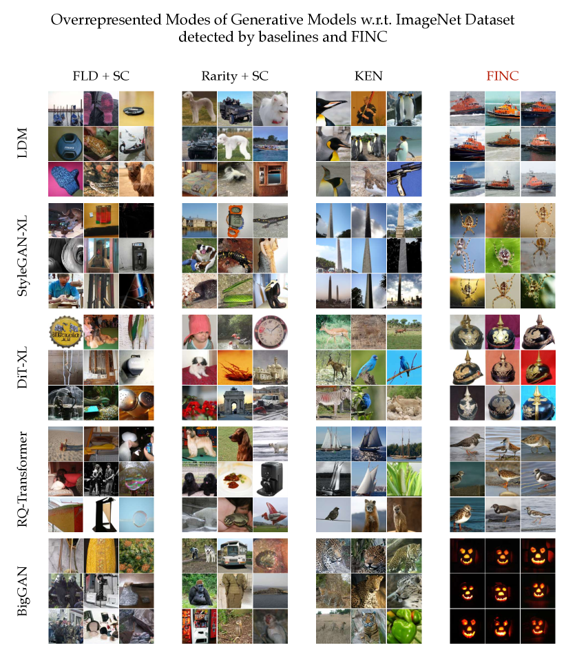
Figure 8: Baseline-identified and FINC-identified top overrepresented modes expressed by test generative models with a considerably higher frequency than in the reference ImageNet dataset.

Figure 9: Baseline-identified and FINC-identified novel modes of AFHQ with respect to ImageNet-dog dataset.

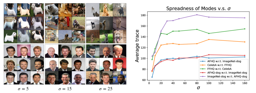
Figure 10: Effect analysis of hyperparameter $\sigma$. Modes captured by smaller $\sigma$ are more specific with similar samples and lower spreadness statistic, while modes captured by larger $\sigma$ are more general with diverse samples and higher spreadness statistic.

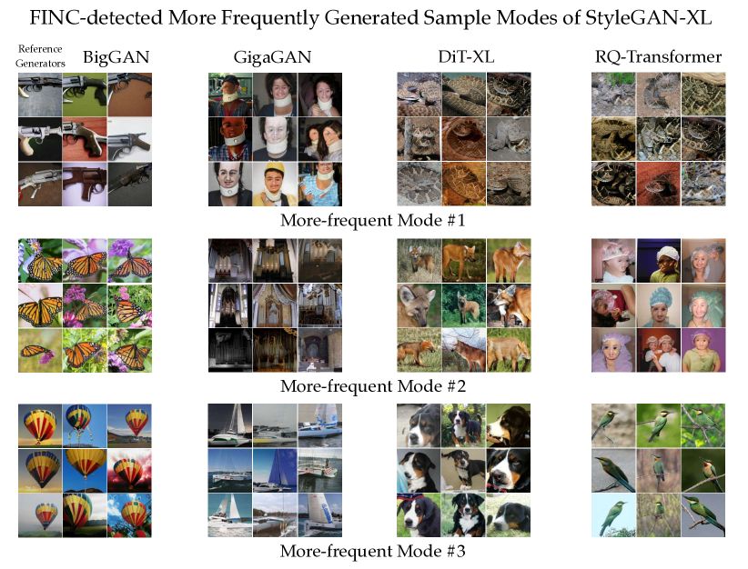
Figure 11: Representative samples from FINC-detected top-3 modes with the maximum frequency gap between StyleGAN-XL (higher frequency) and reference generative models.

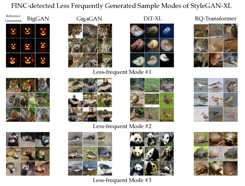
Figure 12: Representative samples from FINC-detected top-3 modes with the maximum frequency gap between StyleGAN-XL (lower frequency) and reference generative models.

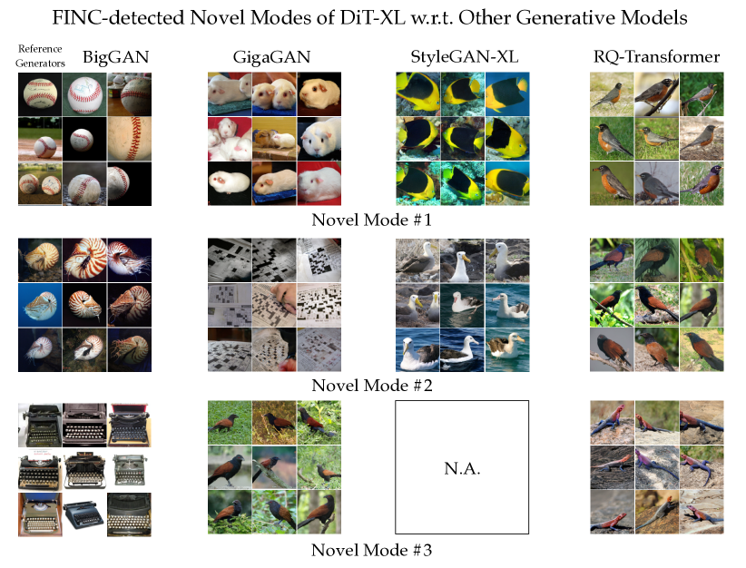
Figure 13: Representative samples from FINC-detected top-3 novel modes (novelty threshold $\rho=5$) of DiT-XL compared to reference generative models. ”N.A.” indicates that DiT-XL has fewer than three modes with a frequency $\rho=5$ times higher than the reference model. Additionally, it is worth noting that FINC does not detect any modes of DiT-XL with a frequency $\rho=5$ times higher than that of LDM.

B.1 Qualitative Comparison between baselines and FINC on ImageNet and AFHQ Dataset

To compare the differential clustering results between the novelty score-based baseline methods and our proposed FINC method, we considered the baseline methods following the FLD score [20], Rarity score [14], and KEN score [48]. In the experiments concerning the FLD and Rarity score-based baselines, we used the methods to detect novel samples, and subsequently we performed the built-in spectral clustering from PyTorch. For the baseline methods, we utilized the largest sample size 10k which did not lead to the memory overflow issue.

Figure 8 presents our numerical results on the ImageNet dataset, suggesting that the novel sample clusters in the Rarity score and FLD baselines may be semantically dissimilar in some cases. On the other hand, we observed that the novel samples within the clusters found by the KEN-based baseline method are more semantically similar. However, a few clusters found by the KEN method may contain more than one mode. However, the proposed FINC method seems to perform a semantically meaningful clustering of the modes in the large-scale ImageNet setting.

We also performed experiments on the AFHQ dataset containing only 15k images that is fewer than 1.4 million images in ImageNet-1K. The baseline methods FLD and KEN methods seemed to perform with higher accuracy on the AFHQ dataset in comparison to the ImageNet-1K dataset. As displayed in Figure 9, FLD seems capable of detecting cat-like modes. The proposed FINC and baseline KEN methods led to nearly identical found modes.

B.2 Analyzing the Effect of $\sigma$ Hyperparameter

We examined the effect of $\sigma$ hyper-parameter of the Gaussian kernel in (1). Based on our numerical evaluations shown in Figure 10, the choice of $\sigma$ could affect the found mode types and statistical heterogeneity within each detected mode. We used the trace of the covariance matrix to measure the heterogeneity of samples within each mode. We observed that smaller values of $\sigma$ could capture more specific modes containing samples with a seemingly lower variety. On the other hand, a greater $\sigma$ value seemed to better capture more general modes, displaying diverse samples and a higher variance statistic.

B.3 Comparative Mode Frequency Analysis between Generative Models

B.3.1 Evaluation of StyleGAN-XL on ImageNet.

Figures 11 and 12 illustrate the more frequently and less frequently generated modes of StyleGAN-XL in comparison to the reference models. These figures repeat the experiments presented in Figures 4 and 5 on StyleGAN-XL.

B.3.2 Novel Modes of DiT-XL on ImageNet.

Figure 13 illustrates the novel modes of DiT-XL with novelty threshold $\rho=5$ in comparison to the reference models. For this experiment, we use a sample size of 100k in each distribution.

B.4 Experimental Results on Text-to-Image Models

Evaluation of text-to-image Models We assessed GigaGAN [21], a state-of-the-art text-to-image generative model on the MS-COCO dataset [27]. We conducted a zero-shot evaluation on the 30K images from the MS-COCO validation set. As shown in Figure 15, the model showed some novelty in generating pictures of a bathroom and sea with a bird or human on it. However, our FINC-based evaluation suggests that the model may be less capable in producing images of zebras, giraffes, or trains.

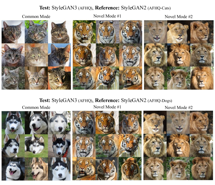
Figure 14: Identified top-2 novel modes and the most common mode between the StyleGAN3 and StyleGAN2 trained on AFHQ

Novel Mode #1

Novel Mode #2

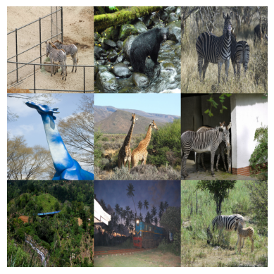
Less-frequent Mode #1

Less-frequent Mode #2

Figure 15: Identified top-2 novel modes and top-2 less-frequent modes on the GigaGAN text-to-image model generated on the MS-COCO dataset.

B.4.1 Effect of different feature extractors

As shown in the literature [24], Inception-V3 may lead to a biased evaluation metric. In this experiment, instead of using pre-trained Inception-V3 to extract features, we used pre-trained models SwAV [7] and ResNet50 [15] as feature extractors and attempted to investigate the effect of different pre-trained models on our proposed method. Figure 16 shows top-3 novel models of GigaGAN [21] using SwAV and ResNet50 models. The top two novel modes were the same among the different feature extractors indicating that our method is not biased on the pre-trained networks. In the third mode, SwAV and ResNet50 results were different showing that each of these models captured different novel modes based on the features they extracted from the data.

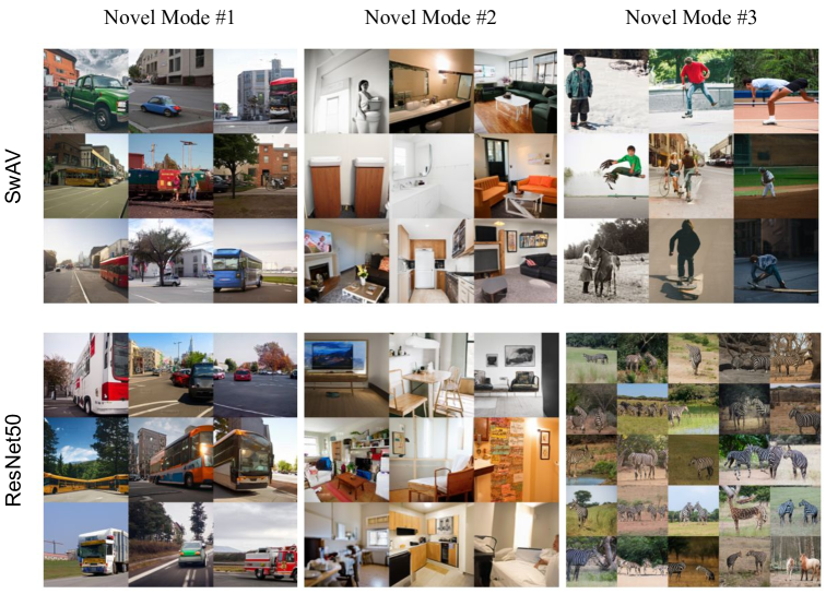
Figure 16: Identified top-3 novel modes on the GigaGAN text-to-image model generated on the MS-COCO dataset using SwAV and ResNet50 pre-trained models as feature extractors.

References

- [1] Alaa, A., Van Breugel, B., Saveliev, E.S., van der Schaar, M.: How faithful is your synthetic data? sample-level metrics for evaluating and auditing generative models. In: International Conference on Machine Learning. pp. 290–306. PMLR (2022)
- [2] Barron, M., Zhang, S., Li, J.: A sparse differential clustering algorithm for tracing cell type changes via single-cell rna-sequencing data. Nucleic acids research 46(3), e14–e14 (2018)
- [3] Bińkowski, M., Sutherland, D.J., Arbel, M., Gretton, A.: Demystifying mmd gans. arXiv preprint arXiv:1801.01401 (2018)
- [4] Bochner, S.: Lectures on fourier integrals. Princeton University Press (1949)
- [5] Borji, A.: Pros and cons of gan evaluation measures: New developments. Computer Vision and Image Understanding 215, 103329 (2022)
- [6] Brock, A., Donahue, J., Simonyan, K.: Large scale gan training for high fidelity natural image synthesis. arXiv preprint arXiv:1809.11096 (2018)
- [7] Caron, M., Misra, I., Mairal, J., Goyal, P., Bojanowski, P., Joulin, A.: Unsupervised learning of visual features by contrasting cluster assignments (2021)
- [8] Child, R.: Very deep vaes generalize autoregressive models and can outperform them on images. arXiv preprint arXiv:2011.10650 (2020)
- [9] Chitta, R., Jin, R., Jain, A.K.: Efficient kernel clustering using random fourier features. In: 2012 IEEE 12th International Conference on Data Mining. pp. 161–170. IEEE (2012)
- [10] Choi, Y., Uh, Y., Yoo, J., Ha, J.W.: Stargan v2: Diverse image synthesis for multiple domains. In: Proceedings of the IEEE/CVF conference on computer vision and pattern recognition. pp. 8188–8197 (2020)
- [11] Deng, J., Dong, W., Socher, R., Li, L.J., Li, K., Fei-Fei, L.: Imagenet: A large-scale hierarchical image database. In: 2009 IEEE conference on computer vision and pattern recognition. pp. 248–255. Ieee (2009)
- [12] Friedman, D., Dieng, A.B.: The vendi score: A diversity evaluation metric for machine learning. arXiv preprint arXiv:2210.02410 (2022)
- [13] Goodfellow, I., Pouget-Abadie, J., Mirza, M., Xu, B., Warde-Farley, D., Ozair, S., Courville, A., Bengio, Y.: Generative adversarial nets. Advances in neural information processing systems 27 (2014)
- [14] Han, J., Choi, H., Choi, Y., Kim, J., Ha, J.W., Choi, J.: Rarity score : A new metric to evaluate the uncommonness of synthesized images. In: The Eleventh International Conference on Learning Representations (2023), https://openreview.net/forum?id=JTGimap_-F
- [15] He, K., Zhang, X., Ren, S., Sun, J.: Deep residual learning for image recognition (2015)
- [16] Heusel, M., Ramsauer, H., Unterthiner, T., Nessler, B., Hochreiter, S.: Gans trained by a two time-scale update rule converge to a local nash equilibrium. Advances in neural information processing systems 30 (2017)
- [17] Ho, J., Jain, A., Abbeel, P.: Denoising diffusion probabilistic models. Advances in neural information processing systems 33, 6840–6851 (2020)
- [18] Hoffman, A.J., Wielandt, H.W.: The variation of the spectrum of a normal matrix. In: Selected Papers Of Alan J Hoffman: With Commentary, pp. 118–120. World Scientific (2003)
- [19] Jalali, M., Li, C.T., Farnia, F.: An information-theoretic evaluation of generative models in learning multi-modal distributions. In: Thirty-seventh Conference on Neural Information Processing Systems (2023)
- [20] Jiralerspong, M., Bose, J., Gemp, I., Qin, C., Bachrach, Y., Gidel, G.: Feature likelihood score: Evaluating the generalization of generative models using samples. In: Thirty-seventh Conference on Neural Information Processing Systems (2023), https://openreview.net/forum?id=l2VKZkolT7
- [21] Kang, M., Zhu, J.Y., Zhang, R., Park, J., Shechtman, E., Paris, S., Park, T.: Scaling up gans for text-to-image synthesis. In: Proceedings of the IEEE Conference on Computer Vision and Pattern Recognition (CVPR) (2023)
- [22] Karras, T., Laine, S., Aila, T.: A style-based generator architecture for generative adversarial networks. In: Proceedings of the IEEE/CVF conference on computer vision and pattern recognition. pp. 4401–4410 (2019)
- [23] Kingma, D.P., Welling, M.: Auto-encoding variational bayes. arXiv preprint arXiv:1312.6114 (2013)
- [24] Kynkäänniemi, T., Karras, T., Aittala, M., Aila, T., Lehtinen, J.: The role of imagenet classes in fréchet inception distance. In: The Eleventh International Conference on Learning Representations (2023), https://openreview.net/forum?id=4oXTQ6m_ws8
- [25] Kynkäänniemi, T., Karras, T., Laine, S., Lehtinen, J., Aila, T.: Improved precision and recall metric for assessing generative models. Advances in Neural Information Processing Systems 32 (2019)
- [26] Lee, D., Kim, C., Kim, S., Cho, M., Han, W.S.: Autoregressive image generation using residual quantization. In: Proceedings of the IEEE/CVF Conference on Computer Vision and Pattern Recognition. pp. 11523–11532 (2022)
- [27] Lin, T.Y., Maire, M., Belongie, S., Bourdev, L., Girshick, R., Hays, J., Perona, P., Ramanan, D., Zitnick, C.L., Dollár, P.: Microsoft coco: Common objects in context (2015)
- [28] Liu, Z., Luo, P., Wang, X., Tang, X.: Deep learning face attributes in the wild. In: Proceedings of the IEEE international conference on computer vision. pp. 3730–3738 (2015)
- [29] Luecken, M.D., Theis, F.J.: Current best practices in single-cell rna-seq analysis: a tutorial. Molecular systems biology 15(6), e8746 (2019)
- [30] Meehan, C., Chaudhuri, K., Dasgupta, S.: A non-parametric test to detect data-copying in generative models. In: International Conference on Artificial Intelligence and Statistics (2020)
- [31] Naeem, M.F., Oh, S.J., Uh, Y., Choi, Y., Yoo, J.: Reliable fidelity and diversity metrics for generative models. In: International Conference on Machine Learning. pp. 7176–7185. PMLR (2020)
- [32] Peebles, W., Xie, S.: Scalable diffusion models with transformers. arXiv preprint arXiv:2212.09748 (2022)
- [33] Peng, L., Tian, X., Tian, G., Xu, J., Huang, X., Weng, Y., Yang, J., Zhou, L.: Single-cell rna-seq clustering: datasets, models, and algorithms. RNA biology 17(6), 765–783 (2020)
- [34] Pham, N., Pagh, R.: Fast and scalable polynomial kernels via explicit feature maps. In: Proceedings of the 19th ACM SIGKDD international conference on Knowledge discovery and data mining. pp. 239–247 (2013)
- [35] Phillips, J.: On the uniform continuity of operator functions and generalized powers-stormer inequalities. Tech. rep. (1987)
- [36] Rahimi, A., Recht, B.: Random features for large-scale kernel machines. Advances in neural information processing systems 20 (2007)
- [37] Rahimi, A., Recht, B.: Uniform approximation of functions with random bases. In: 2008 46th annual allerton conference on communication, control, and computing. pp. 555–561. IEEE (2008)
- [38] Rombach, R., Blattmann, A., Lorenz, D., Esser, P., Ommer, B.: High-resolution image synthesis with latent diffusion models (2021)
- [39] Sajjadi, M.S., Bachem, O., Lucic, M., Bousquet, O., Gelly, S.: Assessing generative models via precision and recall. Advances in neural information processing systems 31 (2018)
- [40] Salimans, T., Goodfellow, I., Zaremba, W., Cheung, V., Radford, A., Chen, X., Chen, X.: Improved techniques for training GANs. In: Lee, D., Sugiyama, M., Luxburg, U., Guyon, I., Garnett, R. (eds.) Advances in Neural Information Processing Systems. vol. 29. Curran Associates, Inc. (2016)
- [41] Sauer, A., Schwarz, K., Geiger, A.: Stylegan-xl: Scaling stylegan to large diverse datasets. In: ACM SIGGRAPH 2022 conference proceedings. pp. 1–10 (2022)
- [42] Shmelkov, K., Schmid, C., Alahari, K.: How good is my gan? In: Proceedings of the European conference on computer vision (ECCV). pp. 213–229 (2018)
- [43] Stein, G., Cresswell, J.C., Hosseinzadeh, R., Sui, Y., Ross, B.L., Villecroze, V., Liu, Z., Caterini, A.L., Taylor, J.E.T., Loaiza-Ganem, G.: Exposing flaws of generative model evaluation metrics and their unfair treatment of diffusion models (2023)
- [44] Sutherland, D.J., Schneider, J.: On the error of random fourier features. arXiv preprint arXiv:1506.02785 (2015)
- [45] Szegedy, C., Vanhoucke, V., Ioffe, S., Shlens, J., Wojna, Z.: Rethinking the inception architecture for computer vision. In: Proceedings of the IEEE conference on computer vision and pattern recognition. pp. 2818–2826 (2016)
- [46] Tancik, M., Srinivasan, P., Mildenhall, B., Fridovich-Keil, S., Raghavan, N., Singhal, U., Ramamoorthi, R., Barron, J., Ng, R.: Fourier features let networks learn high frequency functions in low dimensional domains. Advances in Neural Information Processing Systems 33, 7537–7547 (2020)
- [47] Yang, C., Shen, Y., Xu, Y., Zhou, B.: Data-efficient instance generation from instance discrimination. arXiv preprint arXiv:2106.04566 (2021)
- [48] Zhang, J., Li, C.T., Farnia, F.: An interpretable evaluation of entropy-based novelty of generative models. arXiv preprint arXiv:2402.17287 (2024)