Unitarity in the non-relativistic regime and implications for dark matter

Abstract

Unitarity sets upper limits on partial-wave elastic and inelastic cross-sections, which are often violated by perturbative computations. We discuss the dynamics underlying these limits in the non-relativistic regime, namely long-range interactions, and show how the resummation of the elastic 2-particle-irreducible diagrams arising from squaring inelastic processes unitarizes inelastic cross-sections. Our results are model-independent, apply to all partial waves, and affect elastic and inelastic cross-sections, with extensive implications for new physics scenarios, including dark-matter freeze-out and self-interactions.

I Introduction

Unitarity has long stood as a fundamental principle in particle physics, crucially invoked in the past to argue for the existence of then-unknown physics, including the electroweak interactions and the Higgs mechanism Weinberg (1971); Cornwall et al. (1974); Lee et al. (1977).

More recently, it has been extensively employed to circumscribe the range of validity of effective theories aiming to parametrize the still-unknown physics beyond the Standard Model (SM). In this respect, the implications of unitarity have been widely considered in the high-energy limit, relevant for new physics searches at colliders.

In this letter, we consider unitarity in the antipodal limit, the non-relativistic regime Baldes and Petraki (2017). In the forefront of our motivation lies dark matter (DM), which makes up 85% of the non-relativistic matter in our Universe. Besides its phenomenology in today’s Universe, many important cosmological events, such as its production, may also fall within the non-relativistic realm. Our results pertain to the cosmology and astrophysics of DM in a variety of theories at the frontiers of research, but are also more generally applicable to any non-relativistic system.

Unitarity sets upper bounds on partial-wave elastic and inelastic cross-sections that indicate the saturation of the corresponding scattering probability to one. In a theory that is by construction unitary, the ramifications of these bounds are two-fold: ($a$) They may limit unknown physical parameters of interest if phenomenological requirements are imposed that amount to certain processes being sufficiently efficient. ($b$) They may indicate the point where approximations utilized to compute scattering amplitudes fail. While this failure may be simply due to the break-down of a perturbative expansion in a parameter that has become large, in other occasions it hints towards the onset of new phenomena.

In the present work, we reframe these points, posing and answering the following questions: ($a^{\prime}$) What kind of theories give rise to physical processes that can approach or attain the unitarity limits on scattering cross-sections, thereby providing the possibility to approach or attain the bounds on physical parameters set by phenomenological requirements? ($b^{\prime}$) How can we amend perturbative calculations in weakly-coupled unitary theories to ensure they are consistent with unitarity? We begin with reviewing the unitarity limits, before addressing these points and discussing examples in the DM context.

II Off-shell partial-wave optical theorem and unitarity bounds

To minimize technicalities that are tangential to the main goal of this work, we neglect spin in the following. We consider 2-to-2 transition amplitudes that may in general be off-shell, an essential ingredient in our analysis. We expand them into partial waves as follows,

$${\cal M}^{ab}(s,{\bf k}^{a},{\bf k}^{b})=\\ =16\pi\sum_{\ell}(2\ell+1)P_{\ell}({\bf\hat{k}}^{a}\cdot{\bf\hat{k}}^{b}){\cal M}^{ab}_{\ell}(s,|{\bf k}^{a}|,|{\bf k}^{b}|),$$ (1)

where $a$ and $b$ denote the initial and final state, $s$ is the first Mandelstam variable, and ${\bf k}_{a}$ stands for the 3-momentum of each particle in the center-of-momentum (CM) frame in the state $a$. Next, we define the rescaled partial-wave amplitude

$$M^{ab}_{\ell}(s,|{\bf k}^{a}|,|{\bf k}^{b}|)\equiv\sqrt{\dfrac{4|{\bf k}^{a}||{\bf k}^{b}|}{2^{\delta_{a}}2^{\delta_{b}}s}}{\cal M}^{ab}_{\ell}(s,|{\bf k}^{a}|,|{\bf k}^{b}|),$$ (2)

where $\delta_{a}=0$ or 1 if the two particles in the state $a$ are distinguishable or identical respectively. This allows to express 2-to-2 cross-sections in the convenient form $\sigma_{\ell}^{a\to b}=4\sigma_{\ell}^{U}|M_{\ell}^{ab}|^{2}$, where

$$\sigma^{U}_{\ell}\equiv 2^{\delta}\pi(2\ell+1)/{\bf k}^{2},$$ (3)

with the factor $2^{\delta}$ referring to the incoming state.

Following standard methods, but generalizing to off-shell amplitudes Kowalski (1966), $S$-matrix unitarity implies

$${\rm Im} [M^{aa}_{\ell}(s,|{\bf k}|,|{\bf k^{\prime}}|)]=X_{\ell}^{aa}(s,|{\bf k}|,|{\bf k^{\prime}}|)+$$

$$+\sum_{b:~{}\text{on shell}}M^{ab\,*}_{\ell}(s,|{\bf k}|,|{\bf k}^{b}|)M^{ab}_{\ell}(s,|{\bf k^{\prime}}|,|{\bf k}^{b}|),$$ (4)

where in the second line, the 2-particle states $b$ must be on-shell, therefore $|{\bf k}^{b}|$ is determined by $s$. $X_{\ell}^{ab}(s,|{\bf k}|,|{\bf k^{\prime}}|)$ encompasses the contributions of the $2\to n\geqslant 3$ scatterings, notably with the property that $X_{\ell}^{aa}(s,|{\bf k}|,|{\bf k}|)\geqslant 0$. This leads to the important observation that the sign of the imaginary part of the elastic amplitude is not arbitrary; Eq. 4 implies ${\rm Im}[M^{aa}_{\ell}(s,|{\bf k}|,|{\bf k}|)]\geqslant 0$, a fact that will prove critical in the following. Equation 4 can be considered as a generalization of the optical theorem, that we shall employ in different ways in the following.

Specializing to on-shell in and out states sets $|{\bf k}|=|{\bf k}^{\prime}|$ in Eq. 4, which then implies

$${\rm Im}(M^{aa}_{\ell})\geqslant\sum_{b}|M^{ab}_{\ell}|^{2}\geqslant|M^{aa}_{\ell}|^{2}.$$ (5)

This can be recast for $M^{\rm elas}_{\ell}=M^{aa}_{\ell}$ as $|M^{\rm elas}_{\ell}-\mathbb{i}/2|\leqslant 1/2$, which is the familiar unitarity circle centered at $\mathbb{i}/2$ on the complex plane. Moreover, we obtain a combined upper limit on partial-wave elastic and inelastic cross-sections,

$$\sigma^{\rm inel}_{\ell}/\sigma^{U}_{\ell}\leqslant\sqrt{\sigma^{\rm elas}_{\ell}/\sigma^{U}_{\ell}}\left(2-\sqrt{\sigma^{\rm elas}_{\ell}/\sigma^{U}_{\ell}}\right).$$ (6)

The above encompasses the individual bounds $\sigma^{\rm inel}_{\ell}\leqslant\sigma^{U}_{\ell}$ and $\sigma^{\rm elas}_{\ell}\leqslant 4\sigma^{U}_{\ell}$. The unitarity circle, the combined bound on elastic and inelastic cross-sections, and the mapping between them are depicted in Fig. 1.

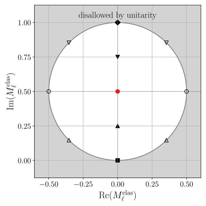
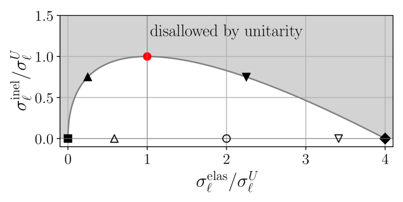
Figure 1: Upper: The unitarity circle bounding the on-shell partial-wave elastic matrix elements $M^{\rm elas}_{\ell}$. The border of the circle corresponds to vanishing inelasticity. Lower: Combined bound on the partial-wave elastic and inelastic cross-sections. The symbols identify points between the two plots. The filled red circle corresponds to maximum inelastic scattering.

III The physics of the unitarity limit, and unitarity violation

The dependence of the cross-section (3) on the kinematic variables allows us to address question $(a^{\prime})$. Let us first motivate this phenomenologically with an example.

Reference Griest and Kamionkowski (1990) argued that the upper bounds on the inelastic cross-sections imply an upper bound on the mass of thermal-relic DM. The calculation amounted to bounding the so-called canonical DM annihilation cross-section by the inelastic $s$-wave unitarity limit, $\sigma_{\rm can}v_{\rm rel}=2.2\times 10^{-26}{\rm cm^{3}/s}<4\pi/(m^{2}v_{\rm rel})$, where $|{\bf k}|=mv_{\rm rel}/2$ in the non-relativistic regime, with $m$ and $v_{\rm rel}$ being the mass and relative velocity of the interacting particles. In this comparison, there is clearly a discrepancy between the velocity scaling of $\sigma_{\rm can}$ and $\sigma_{0}^{U}$. Reference Griest and Kamionkowski (1990) claimed that the momentum scaling of $\sigma_{\ell}^{U}$ cannot be obtained in the non-relativistic regime (and simply used a typical value during freeze-out, $v_{\rm rel}\sim 0.5$, to evaluate $\sigma^{U}_{0}$), and that $s$-wave annihilation dominates. This however, is not so, as unitarity implies Baldes and Petraki (2017); von Harling and Petraki (2014) and as we shall now discuss.

In the relativistic regime, $|{\bf k}|\to\sqrt{s}/2$, which leads to the well-known conclusion that cross-sections should decrease with energy at least as fast as $\sigma\propto 1/s$ at sufficiently high energies. Indeed, for a process computed within an effective theory where the effect of a large scale $\Lambda$ has been integrated out, the cross-section scales typically as $\sigma\sim s/\Lambda^{4}$. Unitarity then implies that the effective theory breaks down at $s\gtrsim\Lambda^{2}$, where the high-energy physics must be resolved and incorporated in the computation. This may involve, for example, the dynamical $s$-channel propagation of a mediator, which restores the scaling $\sigma\sim 1/s$. Then, approaching or attaining the unitarity limit amounts essentially to the couplings involved being sufficiently large, and if this is so, it will hold for the semi-infinite range of energies (or momenta), $s\gtrsim\Lambda^{2}$.

In the non-relativistic regime, such an effective theory fails if $s\gtrsim\Lambda^{4}/|{\bf k}|^{2}$. Setting $s\simeq 4m^{2}$ and $|{\bf k}|\simeq mv_{\rm rel}/2$, implies that the failure is due to the hierarchy $m>\Lambda$. A resolution similar to before may establish again the scaling $\sigma\propto 1/s<1/|{\bf k}|^{2}$. While this respects unitarity as we move to lower $|{\bf k}|$, it does not provide the possibility to approach or attain the unitarity limit at a semi-infinite range of momenta, $|{\bf k}|<m$.

However, the hierarchy $m>\Lambda$ suggests that a new effect may become important, namely that the underlying interaction may manifest as long-ranged Hisano et al. (2003), in the sense that its range, $\lambda_{\rm inter}\propto 1/\Lambda$ may be comparable to or longer than the de Broglie wavelength of the interacting particles, $\lambda_{B}\sim 1/|{\bf k}|$. (Another scale is in fact relevant in this comparison, the analogue of the Bohr radius, where $v_{\rm rel}$ is replaced by the strength of the interaction, see Baldes and Petraki (2017) for more details.) If this is so, the resulting self-interaction between the incoming particles, which could be for example the $t$-channel exchange of a mediator, must be resummed, to account for their interactions at infinity. The distortion of the wavefunction due to this interaction reproduces the momentum scaling of $\sigma_{\ell}^{U}$ if the interaction is sufficiently long-ranged and attractive, as is known for the Coulomb potential, or even shorter-ranged potentials in the regime where they can be approximated by Coulomb (see e.g. Petraki et al. (2017)). Then, if the interaction is also sufficiently strong, it may approach or attain the unitarity limit in the non-relativistic regime, for a semi-infinite momentum range at $|{\bf k}|<m$ Baldes and Petraki (2017); von Harling and Petraki (2014).

Returning to the earlier phenomenological example, we may conclude that thermal-relic DM can be as heavy as unitarity allows only if it possesses attractive long-range interactions Baldes and Petraki (2017). Such interactions imply the existence of bound states, and it has been shown that the formation and decay of metastable bound states in the early Universe can deplete DM very efficiently von Harling and Petraki (2014), also via higher partial waves Baldes and Petraki (2017). Which and how many partial waves are important depends on the model adopted, there is thus no model-independent upper bound on the mass of thermal-relic DM. Nevertheless, considering carefully the unitarity limit has allowed us to understand, in a model-independent fashion, what is the underlying physics of viable heavy, thermal-relic DM models.

While resummation always ensures that elastic cross-sections respect unitarity, state-of-the-art computations still violate the inelastic unitarity bounds at some level. These include: (i) In theories with attractive long-range interactions, typically generated by one-boson exchange diagrams, the Coulomb potential produces cross-sections with the same momentum dependence as $\sigma_{\ell}^{U}$. However inelastic unitarity is violated at sufficiently large couplings. In a QED-like theory, this occurs at $\alpha\gtrsim 0.85$, considering the dominant $s$- and $p$-wave processes for a fermion-antifermion pair Petraki et al. (2017). (ii) In more complex models, bound states may form from scattering states that have a different potential than the bound states, e.g. bound-state formation with emission of a charged scalar Oncala and Petraki (2020, 2021a, 2021b); Ko et al. (2020) or a non-Abelian gauge boson Harz and Petraki (2018); Binder et al. (2023). As a result, the cross-sections exhibit non-monotonic dependence on the incoming momentum, with peaks that can violate unitarity for a finite velocity range, even for fairly small values of the couplings. The problem is exacerbated if the potential in the initial state is repulsive Oncala and Petraki (2020); Binder et al. (2023). (iii) Theories with light but massive mediators possess (nearly) parametric resonances at the thresholds for the existence of bound levels, where inelastic cross-sections scale as $\sigma v_{\rm rel}\propto v_{\rm rel}^{-2}$ at low $v_{\rm rel}$, and violate unitarity at sufficiently low $v_{\rm rel}$ Cassel (2010); Petraki et al. (2017).

These issues highlight a limitation in our understanding of this regime; they also hamper phenomenological studies of, for example, heavy thermal-relic DM or self-interacting DM, both of which feature long-range interactions. This brings us to question $(b^{\prime})$.

IV Resummation

The inequalities (5) cannot be satisfied if the amplitudes are calculated at any finite order in perturbation theory, as the two sides would then be of different order in the couplings of the theory. This suggests that to ensure consistency with unitarity, we must resum all interactions of interest.

The resummation amounts to a Dyson-Schwinger equation for the 4-point function of the two interacting particles with the kernel being the sum of the 2-particle-irreducible (2PI) diagrams; the latter are defined as those that cannot be cut to give two individual contributions to the same 4-point function. The Dyson-Schwinger equation yields the Bethe-Salpeter equation for the two-particle wavefunction, which reduces to the Schrödinger equation under the instantaneous and non-relativistic approximations (see e.g. Petraki et al. (2015) for precise definitions and derivations). In momentum space, it reads

$$\left(\dfrac{{\bf p}^{2}}{2\mu}-{\cal E}_{\bf k}\right)\tilde{\psi}_{\bf k}({\bf p})=\dfrac{1}{4m_{t}\mu}\!\int\!\dfrac{d^{3}p^{\prime}}{(2\pi)^{3}}{\cal A}^{\rm 2PI}(s,{\bf p,p^{\prime}})\tilde{\psi}_{\bf k}({\bf p^{\prime}}),$$ (7)

with ${\cal E}_{\bf k}={\bf k}^{2}/(2\mu)$ being the kinetic energy of the system in the CM frame. Here, $m_{t}$ and $\mu$ stand for the total and reduced masses of the interacting particles. Equation 7 can be Fourier transformed to position space using

$$\psi_{\bf k}({\bf r}) =\int\dfrac{d^{3}p}{(2\pi)^{3}}\,e^{\mathbb{i}{\bf p\cdot r}}\tilde{\psi}_{\bf k}({\bf p}),$$ (8)

$${\cal V}({\bf r,r^{\prime}}) =\dfrac{-1}{4m_{t}\mu}\int\!\dfrac{d^{3}p}{(2\pi)^{3}}\dfrac{d^{3}p^{\prime}}{(2\pi)^{3}}\,e^{\mathbb{i}{\bf p\cdot r}}{\cal A}^{\rm 2PI}(s,{\bf p,p^{\prime}})\,e^{-\mathbb{i}{\bf p^{\prime}\cdot r^{\prime}}},$$ (9)

where we left the dependence of ${\cal V}({\bf r,r^{\prime}})$ on $s$ implicit.

Two important remarks are in order. First, no on-shell condition should be imposed on the 2PI amplitude, ${\cal A}^{\rm 2PI}(s,{\bf p,p^{\prime}})$. Note that when on-shell, $|{\bf p}|=|{\bf p^{\prime}}|$ are determined by $s$. In fact, in the instantaneous approximation, the dependence of ${\cal A}^{\rm 2PI}$ on the energy transfer is neglected (cf. ref. Petraki et al. (2015)). In position space this yields, in general, non-local potentials ${\cal V}({\bf r,r^{\prime}})$. Second, guided by the generalized optical theorem (4), we do not restrict our analysis to the case of ${\cal A}^{\rm 2PI}$ depending on ${\bf p-p^{\prime}}$ only, rather than ${\bf p}$ and ${\bf p^{\prime}}$ separately. This assumption would lead to a central potential, where all partial waves are related. We treat instead all partial waves independently, and do not specify the momentum dependence of ${\cal A}^{\rm 2PI}$.

In a weakly coupled system, the potential vanishes at $r\to\infty$ as ${\cal V}({\bf r,r^{\prime}})\sim r^{-(1+\epsilon)}$ with $\epsilon\geqslant 0$. Then, scattering is described by wavefunctions that asymptote to an incoming plane wave plus an outgoing spherical wave at spatial infinity; in position space

$$\psi_{\bf k}({\bf r})\stackrel{{\scriptstyle r\to\infty}}{{\simeq}}e^{\mathbb{i}{\bf k\cdot r}}+f_{\bf k}(\Omega_{\bf r})\dfrac{e^{\mathbb{i}kr}}{r},$$ (10)

where $k=|{\bf k}|$, and $f_{\bf k}(\Omega_{\bf r})$ encodes the scattering dynamics. (For ${\cal V}(r,r^{\prime})\propto 1/r$, $f_{\bf k}$ has a mild $r$ dependence at $r\to\infty$, which does not spoil any of our conclusions.)

As is customary, $\psi_{\bf k}$ and $f_{\bf k}$ may be expanded into partial waves and re-expressed in terms of phase-shifts,

$$\psi_{\bf k}({\bf r}) =\sum_{\ell}(2\ell+1)P_{\ell}({\bf\hat{k}\cdot\hat{r}})\,\psi_{|\bf k|,\ell}(r),$$ (11)

$$f_{\bf k}(\Omega_{\bf r}) =\sum_{\ell}(2\ell+1)P_{\ell}({\bf\hat{k}\cdot\hat{r}})\,f_{|\bf k|,\ell},$$ (12)

$$f_{|\bf k|,\ell} =\dfrac{e^{\mathbb{i}2\Delta_{\ell}(k)}-1}{\mathbb{i}2k},$$ (13)

where the phase shifts $\Delta_{\ell}(k)$ are in general complex. The partial-wave cross-sections are

$$\dfrac{\sigma^{\rm tot}_{\ell}}{\sigma^{U}_{\ell}} =4k\,{\rm Im}f_{|\bf k|,\ell}=2-2{\rm Re}(e^{\mathbb{i}2\Delta_{\ell}}),$$ (14a)

$$\dfrac{\sigma^{\rm elas}_{\ell}}{\sigma^{U}_{\ell}} =4k^{2}|f_{|{\bf k}|,\ell}|^{2}=1+e^{-4{\rm Im}\Delta_{\ell}}-2{\rm Re}(e^{\mathbb{i}2\Delta_{\ell}}),$$ (14b)

$$\dfrac{\sigma^{\rm inel}_{\ell}}{\sigma^{U}_{\ell}} =\dfrac{\sigma^{\rm tot}_{\ell}-\sigma^{\rm elas}_{\ell}}{\sigma^{U}_{\ell}}=1-e^{-4{\rm Im}\Delta_{\ell}}.$$ (14c)

The total cross-section is obtained from the traditional form of the optical theorem and Eq. 14c clearly includes all inelastic channels. The factors $2^{\delta}$ incorporated in $\sigma^{U}_{\ell}$ arise from the (anti)symmetrisation of the wavefunction in the case of identical particles that doubles the strength of the $\ell$ modes that survive; for all other $\ell$ modes, the cross-sections vanish (see e.g. (Oncala and Petraki, 2021b, appendix A)).

To ensure that unitarity is respected by the above solution, we must still show that ${\rm Im}\Delta_{\ell}\geqslant 0$. This is related to the imaginary part of ${\cal A}^{\rm 2PI}$ that we discuss next.

V Imaginary potential from generalized optical theorem

The generalized optical theorem (4) suggests that inelastic processes generate an imaginary ${\cal A}^{\rm 2PI}$ component. Resumming this contribution renders inelastic cross-sections consistent with unitarity, as we show next.

An imaginary potential due to inelastic processes has been previously considered for the purpose of unitarizing $s$-wave annihilation, in Ref. Blum et al. (2016). However, the connection with the generalized optical theorem was not identified, resulting in ambiguity on the sign of the potential, which is an important issue. Moreover, a central potential was adopted, which does not allow to treat different partial waves independently Yamaguchi (1954), and the chosen potential, being a $\delta$-function in position space, amounted to a specific choice for the underlying inelastic interaction. Our treatment handles all partial waves independently, and does not make model assumptions for the momentum dependence of the resummed process. The sole constraint is the generalized optical theorem (4), as it should be.

To obtain ${\rm Im}[{\cal A}^{\rm 2PI}]$, we must remove from the right-hand side of Eq. 4 all elastic contributions (which yield 2-particle-reducible diagrams), and consider only inelastic contributions with any 2PI factors amputated. We denote the latter as ${\cal A}^{{\rm inel},j}$. Note that ${\cal A}^{{\rm inel},j}$ is not the full amplitude for the inelastic channel $j$; the latter requires resummation of the 2PI diagrams of the incoming particles (cf. e.g. Petraki et al. (2015)). For simplicity, we will neglect contributions from $2\to n\geqslant 3$ scattering.

We partial-wave analyze ${\cal A}^{\rm 2PI}$ and ${\cal A}^{{\rm inel},j}$ according to Eq. 1, and define their corresponding rescaled versions, that we shall call $A^{\rm 2PI}_{\ell}$ and $a^{j}_{\ell}$, according to Eq. 2. Then, the generalized optical theorem (4) implies

$${\rm Im}[A^{\rm 2PI}_{\ell}(s,|{\bf k}|,|{\bf k^{\prime}}|)]=\sum_{j}a^{j\,*}_{\ell}(s,|{\bf k}|)\,a^{j}_{\ell}(s,|{\bf k^{\prime}|}),$$ (15)

where we do not specify the final-state momenta in the inelastic factors $a^{j}_{\ell}$ since they are on-shell and determined by $s$. Equation 15 is a key element in our analysis.

To proceed, we transcribe Eq. 15 in position space, according to Eq. 9. We analyze ${\cal V}({\bf r,r^{\prime}})$ in partial waves,

$${\cal V}({\bf r,r^{\prime}})=\sum_{\ell}\dfrac{2\ell+1}{4\pi}P_{\ell}({\bf\hat{r}\cdot\hat{r}^{\prime}}){\cal V}_{\ell}(r,r^{\prime}),$$ (16)

and obtain

$${\rm Im}[{\cal V}_{\ell}(r,r^{\prime})] =-\sum_{j}\nu^{j\,*}_{\ell}(r)\,\nu^{j}_{\ell}(r^{\prime}),$$ (17)

with

$$\nu^{j}_{\ell}(r) =\left(\dfrac{2^{1+\delta}}{\pi^{2}\mu}\right)^{1/2}\int_{0}^{\infty}dp\,p^{3/2}\,j_{\ell}(pr)\,a^{j}_{\ell}(s,p),$$ (18)

where we set $\sqrt{s}\simeq m_{t}$ in the prefactor, consistently with the non-relativistic approximation leading to Eq. 9 Petraki et al. (2015).

With this, we now revisit the phase shifts $\Delta_{\ell}$. We consider the current ${\bf j}_{\bf k}({\bf r})\equiv{\rm Im}[\psi_{\bf k}^{*}({\bf r})\nabla\psi_{\bf k}({\bf r})]/\mu$. Using Stokes’ theorem and the continuity equation,

$$\sigma^{\rm inel} =-\dfrac{\mu}{k}\int d^{3}r\,\nabla\cdot{\bf j}_{\bf k}({\bf r})$$

$$=2\ {\rm Im}\left[\int d^{3}rd^{3}r^{\prime}\,\psi_{\bf k}^{*}({\bf r}){\cal V}({\bf r,r^{\prime}})\psi_{\bf k}({\bf r^{\prime}})\right].$$ (19)

Using the first Born approximation for the right-hand side, and expanding correspondingly the left-hand side in ${\rm Im}\Delta_{\ell}$, keeping lowest order terms, we find

$$\sum_{\ell}4\sigma^{U}_{\ell}{\rm Im}\Delta_{\ell}(k)\simeq\dfrac{1}{2m_{t}k}{\rm Im}[{\cal A}^{\rm 2PI}(s,k,k)],$$ (20)

which implies ${\rm Im}\Delta_{\ell}\geqslant 0$ as per Eq. 15. (This remains so if we include $2\to n\geqslant 3$ contributions to ${\rm Im}[{\cal A}^{\rm 2PI}]$.) While this proof is at leading order in the couplings that give rise to inelastic scattering, and concerns the sum of all inelastic processes, we will show how the resummation of Eq. 15 ensures that unitarity is respected at all orders and by the exclusive inelastic cross-sections.

The above analysis, distilled in Eqs. 14, 15 and 20, shows that the resummation of the imaginary part of the 2PI diagrams — which arises from squaring inelastic processes, an essential point — ensures that the inelastic cross-sections are also consistent with unitarity. Much like the real potential, the imaginary one affects both the elastic and inelastic cross-sections.

VI Unitarization of exclusive partial-wave cross-sections

Next, we compute how the consistent resummation of the inelastic contributions to elastic scattering, and in particular of Eq. 15, unitarizes the partial-wave elastic and exclusive inelastic processes.

The cross-section for an inelastic channel $j$ is $\sigma^{{\rm inel},j}_{\ell}=4\sigma^{U}_{\ell}|M^{{\rm inel},j}_{\ell}|^{2}$, where $M^{{\rm inel},j}_{\ell}$ is the corresponding amplitude rescaled according to Eq. 2, that incorporates both the hard-scattering inelastic amplitude, $a^{j}_{\ell}$, and the effect of the non-relativistic potential on the incoming particles,

$$M^{{\rm inel},j}_{\ell}(k) =\dfrac{k^{1/2}}{2\pi^{2}}\int_{0}^{\infty}dp\,p^{3/2}\,\tilde{\psi}_{|{\bf k}|,\ell}(p)\,a^{j}_{\ell}(s,p)$$

$$=\sqrt{\dfrac{2\mu k}{2^{\delta}}}\int_{0}^{\infty}dr\ r^{2}\ \psi_{|{\bf k}|,\ell}(r)\nu^{j}_{\ell}(r).$$ (21)

We shall consider a complex potential whose real part we take to be central for simplicity, ${\rm Re}{\cal V}({\bf r,r^{\prime}})=V(r)\delta^{3}({\bf r-r^{\prime}})$, while its imaginary part is given by Eq. 17. Then, the partial-wave Schrödinger equation for $u_{|{\bf k}|,\ell}(r)\equiv kr\,\psi_{|{\bf k}|,\ell}(r)$ reads

$${\cal S}_{\ell}(r)u_{k,\ell}(r)-\mathbb{i}\sum_{j}r\,\nu^{j*}_{\ell}(r)\int_{0}^{\infty}\!\!dr^{\prime}r^{\prime}\nu^{j}_{\ell}(r^{\prime})\,u_{k,\ell}(r^{\prime})=\\ ={\cal E}_{\bf k}u_{k,\ell}(r),$$ (22)

where ${\cal S}_{\ell}(r)$ is the differential operator

$${\cal S}_{\ell}(r)\equiv-\dfrac{1}{2\mu}\dfrac{d^{2}}{dr^{2}}+\dfrac{\ell(\ell+1)}{2\mu\,r^{2}}+V(r),$$ (23)

and ${\cal E}_{\bf k}={\bf k^{2}}/(2\mu)$, as before. We define two versions of the amplitudes and cross-sections: the unregulated ones, for which we neglect the imaginary potential, and the regulated ones, for which we take into account the entire complex potential. We denote them by the subscripts ‘unreg’ and ‘reg’ respectively, and emphasize that both versions include the effect of the real part of the potential. We aim to express the latter in terms of the former.

To do so, we consider the solution of Schrödinger’s equation in the former case and the Green’s function,

$$\left[{\cal S}_{\ell}(r)-{\cal E}_{\bf k}\right]{\cal F}_{k,\ell}(r) =0,$$ (24)

$$\left[{\cal S}_{\ell}(r)-{\cal E}_{\bf k}\right]G_{k,\ell}(r,r^{\prime}) =\delta(r-r^{\prime}).$$ (25)

We require that the asymptotic behaviour of ${\cal F}_{k,\ell}(r)$ at $r\to\infty$ is that of an incident plane wave plus an outgoing spherical wave while $G_{k,\ell}(r,r^{\prime})$ acts as an outgoing spherical wave at large $r$. For some well-known real potentials, ${\cal F}_{k,\ell}$ and $G_{k,\ell}$ are known functions. For any theory, the latter can be expressed in terms of the former,

$$G_{k,\ell}(r,r^{\prime})=\frac{2\mu}{2^{\delta}\pi}\int_{-\infty}^{\infty}dq\ \frac{{\cal F}_{q,\ell}(r){\cal F}_{q,\ell}^{*}(r^{\prime})}{q^{2}-k^{2}-\mathbb{i}\epsilon},$$ (26)

with $\epsilon\to 0^{+}$. We also define the normalization matrix

$$[\mathbb{N}_{\ell}(k)]^{ij}\equiv\delta^{ij}-\mathbb{i}\int_{0}^{\infty}dr\ r\ dr^{\prime}r^{\prime}\nu_{\ell}^{i}(r)G_{k,\ell}(r,r^{\prime})\nu_{\ell}^{j*}(r^{\prime}).$$ (27)

With this, we find that the solution to Eq. 22 is

$$u_{k,\ell}(r)={\cal F}_{k,\ell}(r) +\mathbb{i}\sqrt{\dfrac{2^{\delta}k}{2\mu}}\sum_{i,j}M_{\ell,\rm unreg}^{{\rm inel},j}(k)[\mathbb{N}_{\ell}^{-1}(k)]^{ij}\times$$

$$\times\int_{0}^{\infty}dr^{\prime}\,r^{\prime}\,G_{k,\ell}(r,r^{\prime})\nu_{\ell}^{i*}(r^{\prime}).$$ (28)

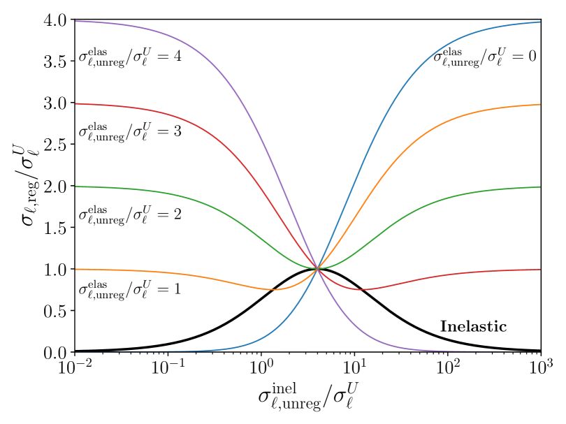
Figure 2: The regulated elastic (colored lines) and 2-to-2 inclusive inelastic (black line) partial-wave cross-sections, vs the unregulated 2-to-2 inclusive inelastic cross-section.

If the unregulated amplitudes are analytic in the entire complex-momentum plane and vanish at complex infinity, then we can evaluate the integral in Eq. 27 using (26), and express it in terms of the unregulated amplitudes. Then, Eqs. 21 and VI allow us to obtain the regulated cross-sections in terms of the unregulated ones. Defining $x_{\ell,\rm(un)reg}\equiv\sigma^{\rm elas}_{\ell,\rm(un)reg}/\sigma_{\ell}^{U}$, $y_{\ell,\rm(un)reg}^{j}\equiv\sigma^{{\rm inel},j}_{\ell,{\rm(un)reg}}/\sigma^{U}_{\ell}$ and $y_{\ell,\rm(un)reg}\equiv\sum_{j}y_{\ell,\rm(un)reg}^{j}$, we find

$$x_{\ell,\rm reg} =\dfrac{x_{\ell,\rm unreg}(1-y_{\ell,\rm unreg}^{2}/16)+y_{\ell,\rm unreg}^{2}/4}{\left(1+y_{\ell,\rm unreg}/4\right)^{2}},$$ (29a)

$$y_{\ell,\rm reg}^{j} =\dfrac{y_{\ell,\rm unreg}^{j}}{\left(1+y_{\ell,\rm unreg}/4\right)^{2}}.$$ (29b)

Full derivations are given in the supplemental material.

Equation 29 are manifestly consistent with unitarity, $x_{\ell,\rm reg}\leqslant 4$ and $y_{\ell,\rm reg}^{j}\leqslant y_{\ell,\rm reg}\leqslant 1$. (Note that $x_{\ell,\rm unreg}\leqslant 4$ since it already includes resummation of ${\rm Re}[{\cal A}^{\rm 2PI}]$.) The combined bound (6) is also respected. The maximum inelastic cross-section is reached for $y_{\ell,\rm unreg}=4$, where, consistently with (6), $x_{\ell,\rm reg}=y_{\ell,\rm reg}=1$, irrespectively of $x_{\ell,\rm unreg}$ (cf. Fig. 1). We plot Eq. 29 in Fig. 2. Their ramifications are far-reaching:

• The resummation of the squared inelastic diagrams affects rather significantly both the inelastic and elastic cross-sections. It is thus expected to affect the computations of the DM density in various production mechanisms, as well as those of the DM self-interaction cross sections; the latter can affect the galactic structure (see Tulin and Yu (2018); Bullock and Boylan-Kolchin (2017) for reviews).

• Each inelastic channel is regulated by the inclusive inelastic cross-section. It follows that even if a certain inelastic channel appears seemingly irrelevant for a particular purpose due to its nature, it may in fact be very important, provided that it is sufficiently strong. This is because such a process regulates the pertinent inelastic processes.

  For example, in DM freeze-out, metastable bound-state formation processes that are comparable to or faster than direct annihilation into radiation can significantly renormalize down the strength of the latter (cf. Ref. (Oncala and Petraki, 2021b, Fig. 11)), even when they themselves cannot deplete DM efficiently due to their rapid dissociation by the radiation bath. This may suppress the DM depletion and alter predictions.

• For $y_{\ell,\rm unreg}\ll 1$, the relative corrections to the scattering rates are $\delta x_{\ell}/x_{\ell}\simeq\delta y_{\ell}^{j}/y_{\ell}^{j}\simeq y_{\ell,\rm unreg}/2$.

  For DM freeze-out, this implies that the imaginary potential affects the DM density at a level similar to or larger than the experimental uncertainty if $y_{\ell,\rm unreg}\gtrsim{\cal O}(10^{-2})$, i.e., even when the annihilation cross-section is far below the unitarity limit.

• At the opposite limit, $y_{\ell,\rm unreg}\gg 1$, we find $x_{\ell,\rm reg}\simeq 4-x_{\ell,\rm unreg}$ and $y_{\ell,\rm reg}\simeq 16/y_{\ell,\rm unreg}$, i.e., perhaps counter-intuitively, the regulated cross-sections decrease as the unregulated ones increase. Note that $y_{\ell,\rm unreg}\gg 1$ can occur even at (very) small values of the couplings. This is for example the case for certain BSF processes via monopole Oncala and Petraki (2020, 2021a, 2021b) or dipole Binder et al. (2023) transitions, particularly in models where the interaction of the particles in the incoming scattering state is repulsive. It is also so at resonances.

  With respect to the DM density, this implies that there could be two branches of solutions (mass-coupling correlation) that yield the observed value.

• If the unregulated cross-sections exhibit the same momentum dependence as the unitarity limit, then this feature is retained by the regularisation. If not, the regularisation implies a non-trivial velocity dependence. The earlier conclusion thus remains: the unitarity bounds can be realized in the non-relativistic regime for a semi-infinite range of momenta only by attractive long-range interactions.

• The upper bounds implied by unitarity on the mass of frozen-out DM annihilating via a single partial wave $\ell$, or all partial waves in the range $0\leqslant\ell\leqslant L$, are, for self-conjugate and non-self-conjugate DM,
  $m_{\rm uni}/(140\ {\rm TeV})$ solely $\ell$ $0\leqslant\ell\leqslant L$ non-self-conj. DM $\sqrt{1+2\ell}$ $(1+L)$ self-conj. DM $2\sqrt{1+2\ell}$ $2\sqrt{(1+L)\left(1+L/2\right)}$
  where we used the numerical results of von Harling and Petraki (2014); Baldes and Petraki (2017), assuming for definiteness that DM annihilates into plasma of the same temperature as the SM, and any extra relativistic degrees of freedom are negligible with respect to those of the SM. The above results incorporate the factor $2^{\delta}$ of Eq. 3 that affects the bounds for self-conjugate DM but has not been previously appreciated in similar estimations. It also takes into account that for self-conjugate DM, only $\ell$ even or odd modes survive, depending on the statistics. We iterate that there is no model-independent bound on the mass of thermal-relic DM due to unitarity, as which partial waves contribute significantly depends on the model.

VII Conclusions

The violation of inelastic unitarity limits in the non-relativistic regime by state-of-the art computations hampers a variety of phenomenological investigations in the current frontiers of DM research. Resolving this issue is important for improving our theoretical understanding, as well as interpreting and guiding experimental searches.

We have derived a simple analytical regularization scheme, given by Eq. 29, whose input are the inelastic cross-sections as affected only by the real part of the potential, and output are the unitarized elastic and inelastic cross-sections. The scheme applies to any partial wave, and is model-independent as it makes no assumptions about the momentum dependence of the unregulated inelastic amplitudes. This result can be, and must be, employed in investigations of new physics scenarios in the non-relativistic regime, with wide-ranging implications.

Supplemental material

Appendix A Schrödinger equation and regulated amplitudes

We present the solution of Schrödinger’s equation with a real, local potential plus an imaginary potential that is the sum of non-local, separable components of the form of Eq. 17. Similar solutions have been considered in nuclear physics Yamaguchi (1954); McMillan (1963); Shah-Jahan (1973); Joachain (1975); Arellano and Blanchon (2019), though we offer a more general solution that includes the sum of separable potentials.

Schrödinger’s equation for $u_{k,\ell}(r)\equiv kr\psi_{k,\ell}(r)$ reads

$$[{\cal S}_{\ell}(r)-{\cal E}_{\bf k}]u_{k,\ell}(r)=\\ =\mathbb{i}\sum_{j}r\nu_{\ell}^{j*}(r)\int_{0}^{\infty}dr^{\prime}r^{\prime}\nu_{\ell}^{j}(r^{\prime})u_{k,\ell}(r^{\prime}),$$ (30)

where ${\cal S}_{\ell}(r)$ is the differential operator that contains the kinetic term and the real part of the potential, $V(r)\in\mathbb{R}$,

$${\cal S}_{\ell}(r)\equiv-\dfrac{1}{2\mu}\dfrac{d^{2}}{dr^{2}}+\dfrac{\ell(\ell+1)}{2\mu\,r^{2}}+V(r),$$ (31)

and ${\cal E}_{\bf k}={\bf k}^{2}/(2\mu)$. To solve Eq. 30, we first consider the ${\cal S}_{\ell}$ eigenfunctions and Green’s function, defined via

$$\left[{\cal S}_{\ell}(r)-{\cal E}_{\bf k}\right]{\cal F}_{k,\ell}(r) =0,$$ (32a)

$$\left[{\cal S}_{\ell}(r)-{\cal E}_{\bf k}\right]{\cal G}_{k,\ell}(r) =0,$$ (32b)

$$\left[{\cal S}_{\ell}(r)-{\cal E}_{\bf k}\right]G_{k,\ell}(r,r^{\prime}) =\delta(r-r^{\prime}),$$ (32c)

where the ${\cal F}_{k,\ell}$ and ${\cal G}_{k,\ell}$ families of solutions feature different asymptotic behaviors at $r\to\infty$,

$${\cal F}_{k,\ell}(r\to\infty) \mapsto+\frac{1}{\mathbb{i}2}\left(e^{\mathbb{i}kr}e^{\mathbb{i}2\theta_{\ell}(k)}-e^{-\mathbb{i}(kr-\ell\pi)}\right),$$ (33a)

$${\cal G}_{k,\ell}(r\to\infty) \mapsto-\frac{1}{2}\left(e^{\mathbb{i}kr}e^{\mathbb{i}2\theta_{\ell}(k)}+e^{-\mathbb{i}(kr-\ell\pi)}\right).$$ (33b)

with $\theta_{\ell}(k)\in\mathbb{R}$. ${\cal F}_{k,\ell}(r)$ describe states of an incident plane wave plus an outgoing spherical wave, and are the solutions of interest. ${\cal G}_{k,\ell}(r)$ will be useful for computational purposes. We shall require that $G_{k,\ell}(r,r^{\prime})$ acts as an outgoing spherical wave at $r\to\infty$. We may now write an implicit solution for $u_{k,\ell}(r)$ for the full potential,

$$u_{k,\ell}(r)={\cal F}_{k,\ell}(r)+$$ (34)

$$+\mathbb{i}\sqrt{\dfrac{2^{\delta}k}{2\mu}}\sum_{j}M_{\ell,\rm reg}^{{\rm inel},j}(k)\left(\int_{0}^{\infty}dr^{\prime}r^{\prime}G_{k,\ell}(r,r^{\prime})\nu_{\ell}^{j*}(r^{\prime})\right),$$

where we expressed the $r$-independent factor of the second term in terms of the rescaled regulated inelastic amplitudes, which however depend on the wavefunction. We also need the unregulated ones. We recall that

$$M^{{\rm inel},j}_{\ell,\rm unreg}(k) =\sqrt{\dfrac{2\mu}{2^{\delta}k}}\int_{0}^{\infty}dr\,r\,{\cal F}_{k,\ell}(r)\,\nu^{j}_{\ell}(r),$$ (35a)

$$M^{{\rm inel},j}_{\ell,\rm reg}(k) =\sqrt{\dfrac{2\mu}{2^{\delta}k}}\int_{0}^{\infty}dr\,r\,u_{k,\ell}(r)\,\nu^{j}_{\ell}(r).$$ (35b)

Inserting Eq. 34 into (35b), and introducing the matrix

$$[\mathbb{N}_{\ell}(k)]^{ij}\equiv\delta^{ij}-\mathbb{i}\int_{0}^{\infty}dr\,r\,dr^{\prime}r^{\prime}\nu_{\ell}^{i}(r)\,G_{k,\ell}(r,r^{\prime})\,\nu_{\ell}^{j*}(r^{\prime}),$$ (36)

we obtain a matrix equation between regulated and unregulated inelastic amplitudes. Upon inversion, it gives

$$M^{{\rm inel},i}_{\ell,{\rm reg}}(k)=\sum_{j}[\mathbb{N}_{\ell}^{-1}(k)]^{ij}\ M_{\ell,\rm unreg}^{{\rm inel},j}(k).$$ (37)

Equation 37 is the key result of this section: it expresses the regulated inelastic amplitudes in terms of the unregulated ones. Using Eq. 37, the solution (34) can be re-expressed in terms of input parameters only, the imaginary potential and unregulated wavefunctions.

The Green’s function can be expressed as

$$G_{k,\ell}(r,r^{\prime})=\frac{2\mu}{2^{\delta}\pi}\int_{-\infty}^{\infty}dq\ \frac{{\cal F}_{q,\ell}(r){\cal F}_{q,\ell}^{*}(r^{\prime})}{q^{2}-k^{2}-\mathbb{i}\epsilon},$$ (38)

with $\epsilon\to 0^{+}$ and the analytic continuation ${\cal F}_{-q,\ell}(r)=-{\cal F}_{q,\ell}^{*}(r)$. We prove Eq. 38 in the next section. This leads to the following expression for the matrix $\mathbb{N}$,

$$[\mathbb{N}_{\ell}(k)]^{ij}=\delta^{ij}-\frac{\mathbb{i}}{\pi}\int_{-\infty}^{\infty}\frac{M_{\ell,\rm unreg}^{{\rm inel},i}(q)M_{\ell,\rm unreg}^{{\rm inel},j*}(q)}{q^{2}-k^{2}-\mathbb{i}\epsilon}\ q\ dq.$$ (39)

If the unregulated amplitudes are analytic in the entire complex plane and decreasing functions at complex infinity, then we can evaluate the contour integral to give,

$$[\mathbb{N}_{\ell}(k)]^{ij}=\delta^{ij}+M_{\ell,\rm unreg}^{{\rm inel},i}(k)M_{\ell,\rm unreg}^{{\rm inel},j*}(k).$$ (40)

From here, it is easy to demonstrate that the amplitudes $M_{\ell,\rm unreg}^{{\rm inel},j}(k)$ form an eigenvector of $\mathbb{N}_{\ell}(k)$,

$$\sum_{j}[\mathbb{N}_{\ell}]^{ij}M_{\ell,\rm unreg}^{{\rm inel},j}=M_{\ell,\rm unreg}^{{\rm inel},i}\left(1+\frac{\sigma^{{\rm inel}}_{\ell,{\rm unreg}}}{4\sigma^{U}_{\ell}}\right).$$ (41)

The above implies that the regulated amplitude (37) is

$$M_{\ell,\rm reg}^{{\rm inel},i} =\dfrac{M_{\ell,\rm unreg}^{{\rm inel},i}}{1+\sigma^{{\rm inel}}_{\ell,{\rm unreg}}/(4\sigma^{U}_{\ell})},$$ (42)

from where we obtain the regulated exclusive partial-wave inelastic cross-sections quoted in the main text.

Next, we want to determine the elastic cross-section. For this purpose, we need to deduce the complex phase shift $\Delta_{\ell}(k)$ that determines the asymptotic behavior of the partial-wave modes at $r\to\infty$, according to

$$u_{k,\ell}(r\to\infty)\mapsto\dfrac{1}{\mathbb{i}2}\left(e^{\mathbb{i}[kr+2\Delta_{\ell}(k)]}-e^{-\mathbb{i}(kr-\ell\pi)}\right).$$ (43)

We expand our solution, Eq. 34, in the $r\to\infty$ limit, using the Green’s function (57) and considering the asymptotic forms (33a) and (55). We find the asymptotic form (43) with the phase shift being $\Delta_{\ell}=\theta_{\ell}+\delta_{\ell}$, where

$$e^{\mathbb{i}2\delta_{\ell}(k)} =1-2\sum_{i,j}M_{\ell,\rm unreg}^{{\rm inel},i*}(k)[\mathbb{N}_{\ell}^{-1}(k)]^{ij}M_{\ell,\rm unreg}^{{\rm inel},j}(k)$$

$$=1-2\left(\frac{\sigma^{{\rm inel}}_{\ell,{\rm unreg}}/(4\sigma^{U}_{\ell})}{1+\sigma^{{\rm inel}}_{\ell,{\rm unreg}}/(4\sigma^{U}_{\ell})}\right).$$ (44)

Note that ${\rm Re}(\delta_{\ell})=0$ or $\pi/2$ for $\sigma^{{\rm inel}}_{\ell,{\rm unreg}}<4\sigma^{U}_{\ell}$ or $>4\sigma^{U}_{\ell}$ respectively. Given that $\sigma^{\rm tot}_{\ell}/\sigma_{\ell}^{U}=4k{\rm Im}(f_{|{\bf k}|,\ell})$, or

$$\sigma^{{\rm elas}}_{\ell,\rm unreg}/\sigma_{\ell}^{U} =2-2{\rm Re}[e^{\mathbb{i}2\theta_{\ell}(k)}],$$ (45a)

$$(\sigma^{{\rm elas}}_{\ell,\rm reg}+\sigma^{{\rm inel}}_{\ell,\rm reg})/\sigma_{\ell}^{U} =2-2{\rm Re}[e^{\mathbb{i}2\Delta_{\ell}(k)}],$$ (45b)

we arrive, using Eq. 44, at the result in the main text.

Appendix B Green’s function

We seek an expression for $G_{k,\ell}(r,r^{\prime})$ with the asymptotic behavior of an incident plane wave plus outgoing spherical wave at $r\to\infty$. Following Refs. Yamaguchi (1954); McMillan (1963); Shah-Jahan (1973); Joachain (1975); Arellano and Blanchon (2019), we expand the $r$ dependence of $G_{k,\ell}(r,r^{\prime})$ in terms of ${\cal F}_{q,\ell}(r)$, which, being eigenfunctions of the hermitian operator ${\cal S}_{\ell}(r)$, constitute a complete orthonormal set of states with the desired asymptotic behavior,

$$G_{k,\ell}(r,r^{\prime}) =\int_{0}^{\infty}dq\ g_{k,\ell}(q,r^{\prime})\ {\cal F}_{q,\ell}(r).$$ (46)

Then, Eq. 32c becomes

$$\delta(r-r^{\prime}) =\int_{0}^{\infty}dq\ g_{k,\ell}(q,r^{\prime})[S_{\ell}(r)-{\cal E}_{\bf k}]{\cal F}_{q,\ell}(r),$$

$$=\int_{0}^{\infty}dq\ g_{k,\ell}(q,r^{\prime})\left(\dfrac{q^{2}-k^{2}}{2\mu}\right){\cal F}_{q,\ell}(r).$$ (47)

We must now invert the above to obtain $g_{k,\ell}(q,r^{\prime})$. For this, we need the orthonormality relation for ${\cal F}_{q,\ell}(r)$,

$$\int_{0}^{\infty}dr\ {\cal F}_{q,\ell}(r){\cal F}_{q^{\prime},\ell}^{*}(r)=\dfrac{2^{\delta}\pi}{2}\delta(q-q^{\prime}).$$ (48)

Considering this, Eq. 47 yields

$$g_{k,\ell}(q,r) =\dfrac{4\mu}{2^{\delta}\pi}\dfrac{{\cal F}_{q,\ell}^{*}(r)}{q^{2}-k^{2}}.$$ (49)

Then, Eq. 46 becomes

$$G_{k,\ell}(r,r^{\prime})=\dfrac{4\mu}{2^{\delta}\pi}\int_{0}^{\infty}dq\,\dfrac{{\cal F}_{q,\ell}(r){\cal F}_{q,\ell}^{*}(r^{\prime})}{q^{2}-k^{2}-\mathbb{i}\epsilon},$$ (50)

In order to evaluate $G_{k,\ell}(r,r^{\prime})$, it will be convenient to extend the range of integration over $dq$ to $(-\infty,\infty)$. To analytically continue to $q<0$, we consider the asymptotic behaviors (33), and set self-consistently

$$\theta_{\ell}(-q) =-\theta_{\ell}(q)+\ell\pi,$$ (51a)

$${\cal F}_{-q,\ell}(r) =-{\cal F}_{q,\ell}^{*}(r),$$ (51b)

$${\cal G}_{-q,\ell}(r) =+{\cal G}_{q,\ell}^{*}(r).$$ (51c)

With this, Eq. 50 becomes

$$G_{k,\ell}(r,r^{\prime})=\dfrac{2\mu}{2^{\delta}\pi}\int_{-\infty}^{\infty}dq\,\dfrac{{\cal F}_{q,\ell}(r){\cal F}_{q,\ell}^{*}(r^{\prime})}{q^{2}-k^{2}-\mathbb{i}\epsilon},$$ (52)

with the prescription $\epsilon\to 0^{+}$ chosen such that $G_{k,\ell}(r,r^{\prime})$ behaves as an outgoing spherical wave at $r\to\infty$, as will be shown below. Since ${\cal F}_{q,\ell}(r)$ and ${\cal G}_{q,\ell}(r)$ are real up to the same $\ell$- and $q$-dependent but $r$-independent phase,

$${\cal F}_{q,\ell}(r){\cal F}_{q,\ell}^{*}(r^{\prime}) ={\cal F}_{q,\ell}^{*}(r){\cal F}_{q,\ell}(r^{\prime}),$$ (53a)

$${\cal G}_{q,\ell}(r){\cal G}_{q,\ell}^{*}(r^{\prime}) ={\cal G}_{q,\ell}^{*}(r){\cal G}_{q,\ell}(r^{\prime}),$$ (53b)

$${\cal F}_{q,\ell}(r){\cal G}_{q,\ell}^{*}(r^{\prime}) ={\cal F}_{q,\ell}^{*}(r){\cal G}_{q,\ell}(r^{\prime}).$$ (53c)

Here, this implies $G_{k,\ell}(r,r^{\prime})=G_{k,\ell}(r^{\prime},r)$, as expected.

To evaluate Eq. 52, we consider the two independent eigenfunction families of ${\cal S}_{\ell}$, characterized by the asymptotic behaviors Eq. 33. We then define

$${\cal H}_{k,\ell}^{(\pm)}(r)={\cal F}_{k,\ell}(r)\pm\mathbb{i}{\cal G}_{k,\ell}(r).$$ (54)

The functions ${\cal H}_{k,\ell}^{(\pm)}(r)$ have the properties

$${\cal H}_{k,\ell}^{(+)}(r\to\infty) \mapsto-\mathbb{i}e^{+\mathbb{i}(kr+2\theta_{\ell})},$$ (55a)

$${\cal H}_{k,\ell}^{(-)}(r\to\infty) \mapsto+\mathbb{i}e^{-\mathbb{i}(kr-\ell\pi)},$$ (55b)

$${\cal H}_{-k,\ell}^{(\pm)}(r) =-{\cal H}_{k,\ell}^{(\pm)*}(r).$$ (55c)

We invert Eq. 54 to express ${\cal F}_{k,\ell(r)}$ in terms of ${\cal H}_{k,\ell}^{(\pm)}(r)$, which allows to separate Eq. 52 into two integrals,

$$G_{k,\ell}(r,r^{\prime}) =\dfrac{\mu}{2^{\delta}\pi}\int_{-\infty}^{\infty}dq\,\dfrac{{\cal F}_{q,\ell}^{*}(r){\cal H}_{q,\ell}^{(+)}(r^{\prime})}{q^{2}-k^{2}-\mathbb{i}\epsilon}+$$ (56)

$$+\dfrac{\mu}{2^{\delta}\pi}\int_{-\infty}^{\infty}dq\,\dfrac{{\cal F}_{q,\ell}^{*}(r){\cal H}_{q,\ell}^{(-)}(r^{\prime})}{q^{2}-k^{2}-\mathbb{i}\epsilon}.$$

Based on the asymptotic behavior of ${\cal H}_{k,\ell}^{(\pm)}(r)$ we have to carefully chose the contours necessary for evaluation. For $r<r^{\prime}$, the first integral above must be evaluated in the upper-half plane while the second integral must be evaluated in the lower half plane. Considering this, as well as the analytic continuations (51b) and (55c), we can evaluate the contour integrals using the residue theorem. The case where $r>r^{\prime}$ follows a similar logic. Taking also Eq. 53 into account, we find,

$$G_{k,\ell}(r,r^{\prime})=+\frac{2\mu\mathbb{i}}{2^{\delta}k}{\cal F}_{k,\ell}^{*}(r_{<}){\cal H}_{k,\ell}^{(+)}(r_{>}),$$ (57)

where $r_{<}\equiv\min\{r,r^{\prime}\}$ and $r_{>}\equiv\max\{r,r^{\prime}\}$. The necessary asymptotic behaviour of $G_{k,\ell}(r,r^{\prime})$ is made apparent by the appearance of ${\cal H}_{k,\ell}^{(+)}$ in the above expression.