Discretization Error of Fourier Neural Operators

Abstract

Operator learning is a variant of machine learning that is designed to approximate maps between function spaces from data. The Fourier Neural Operator (FNO) is a common model architecture used for operator learning. The FNO combines pointwise linear and nonlinear operations in physical space with pointwise linear operations in Fourier space, leading to a parameterized map acting between function spaces. Although FNOs formally involve convolutions of functions on a continuum, in practice the computations are performed on a discretized grid, allowing efficient implementation via the FFT. In this paper, the aliasing error that results from such a discretization is quantified and algebraic rates of convergence in terms of the grid resolution are obtained as a function of the regularity of the input. Numerical experiments that validate the theory and describe model stability are performed.

41A35, 65T50, 68T07

1 Introduction

1.1 Overview

While most machine learning architectures are designed to approximate maps between finite-dimensional spaces, operator learning is a data-driven method that approximates maps between infinite-dimensional function spaces. These maps appear commonly in scientific machine learning applications such as surrogate modeling of partial differential equations (PDE) or model discovery from data. Fourier Neural Operators (FNOs) [16] are a type of operator learning architecture that parameterize the model directly in function space, naturally generalizing deep neural networks (DNNs). In particular, each hidden layer of an FNO assigns a trainable integral kernel that acts on the hidden states by convolution in addition to the usual affine weights and biases of a DNN. Taking advantage of the duality between convolution and multiplication under Fourier transforms, these convolutional kernels are represented by Fourier multiplier matrices, whose components are optimized during training, along with the regular weights and biases acting in physical space. FNOs have proven to be an effective and popular operator learning method in several PDE application areas including weather forecasting [21], biomedical shape optimization [24], and constitutive modeling [3]. It is thus of interest to study their theoretical properties.

Although FNOs approximate maps between function spaces, in practice, these functions must be discretized. FNOs are discretization invariant in the sense that varying discretizations of the function space data may be used for both training and testing of the model without changing any model parameters. However, the model performs convolutions on the hidden states, and the discretization of the data can affect the accuracy of these convolutions through aliasing error. During a forward pass of the FNO, the discretization errors of each hidden layer will propagate through the subsequent layers of the FNO and may be amplified by nonlinearities. In previous theoretical analyses of the universal approximation (UA) properties of the FNO [11, 12], the consequent discretization error is ignored completely as the states are considered functions rather than discretizations of functions. While this approach to UA is theoretically sound, it leaves the discretization components of the error unquantified in practice. In this paper, we analyze such components of the error both theoretically and experimentally.

The error resulting from performing a single convolution on a grid rather than on a continuum depends on the regularity, or smoothness, of the input function in the Sobolev sense. Thus, to bound the error for an entire FNO, regularity must be maintained as the state passes through the layers of the network, including the nonlinear activation function. In particular, regularity-preserving properties of compositions of nonlinear functions are required. Bounds of this type are given by Moser [19] and form a key component of the proofs in this work. Because the smooth GeLU (Gaussian Error Linear Unit) [7] activation preserve regularity, while the (non-differentiable) ReLU activations do not, the analysis in this paper is confined to the former and extends to other smooth activation functions.

1.2 Contributions

In this paper, we make the following contributions.

1. We bound theoretically the aliasing error that results from approximating the continuum FNO on a grid.

2. We validate this theory concerning the discretization error of the FNO with numerical experiments.

3. We provide heuristics for avoiding the effects of discretization error in practice.

4. We propose an adaptive subsampling algorithm for faster operator learning training.

In Section 2 we set up the framework for our theoretical results. Section 3 studies the discretization error of the FNO theoretically, making contribution (C1). In Section 4 we present numerical experiments that illustrate the theoretical results and proposes an algorithm for adaptively refining the discretization during training. Thus, Section 4 makes contributions (C2, C3, C4). We conclude in Section 5. Some technical details are contained in the appendices.

1.3 Background

Neural networks have been very successful in approximating solutions of partial differential equations using data. Several approaches are used for such models, including physics-informed neural networks (PINNs), constructive networks, and operator learning models. In the case of PINNs, a standard feed-forward machine learning architecture is trained with a loss function involving a constraint of satisfying the underlying PDE [22]. Such models have shown empirical success in many problems of application [5, 4, 10]. One disadvantage of PINNs is that only a single solution of the underlying PDE is approximated. Thus, adapting the model to different initial or boundary conditions often requires retraining it from scratch. Another approach to applying machine learning to PDEs is to construct approximating networks from classical PDE-solver methods. For example, in [8, 9, 17], ReLU neural networks are shown to replicate polynomial approximations and continuous, piecewise-linear elements used in finite element methods exactly; thus, the constructive approximation proofs used for polynomials and finite element methods apply, and the network weights may be constructed exactly. This approach leverages classical approximation theory to support ReLU neural networks, but in the practical setting of data-driven learning, these methods are often less efficient than methods involving training. Both of these two approaches to approximating PDE solution maps require a choice of discretization to approximate an infinite-dimensional operator.

Operator learning is a branch of machine learning that aims to approximate maps between function spaces, which include solution maps defined by partial differential equations (PDEs) [12]. Several operator learning architectures exist, including DeepONet [18], Fourier Neural Operators (FNO) [16], PCA-Net [2], and random features models [20]. Our paper focuses on FNOs, which directly parameterize the model in Fourier space and allow for changes in discretization in both the input and the output functions, potentially allowing for non-uniform grids [15]. In addition, FNO takes advantage of the computational speedup of the FFT to gain additional model capacity with less evaluation time.

Error analysis for operator learning begins with establishing UA: results which guarantee that, for a class of possible maps, a particular choice of model architecture, and a desired maximum error, there exists a parameterization of the model that gives at most that error. UA results are established for a variety of architectures including ReLU NN in [6], DeepONet in [14], FNO in [11], and a general class of neural operators in [12]. Following UA, model size bounds give a worst-case bound on the model parameter sizes required to achieve a certain error threshold for particular classes of problems. These have been established for FNO [11, 13], but the analysis considers the states of the model to be functions on the continuum and ignores the practical requirement of working with a discretized version of the function. In this work, we focus on this source of error.

Perhaps the most conceptually similar work to ours is [1], which addresses the fact that discretizations of neural operators deviate from their continuum counterparts. The authors of [1] introduce an “alias-free” neural operator that bypasses inconsistencies resulting from discretization. In practice, this research direction has led to operator learning frameworks such as Convolutional Neural Operators (CNO) [23], which are not strictly alias-free, but reduce aliasing errors via spatial upsampling. These prior works have empirically shown the benefits and importance of carefully controlling discretization errors in operator learning.

FNOs remain a widespread neural operator architecture, and a theoretical analysis of errors resulting from numerical discretization have so far been missing from the literature. To fill this gap, in this paper we bound the discretization error of FNOs theoretically and perform experiments that provide greater insight into the behavior of this error.

2 Set-Up

In this section, we establish notation for the paper (Subsection 2.1) and define the FNO (Subsection 2.2).

2.1 Notation

Fix integer $m$. Let $|\cdot|$ denote the Euclidean norm on $\mathbb{R}^{m}$ and $\|\cdot\|$ the $L^{2}(\mathbb{T}^{d},\mathbb{R}^{m})$ norm. Here, $\mathbb{T}^{d}$ denotes the $d$-dimensional torus, which we identify with $[0,1]^{d}$ with periodic boundary conditions; we simply write $L^{2}(\mathbb{T}^{d})$ when no confusion will arise. We define the Sobolev space $H^{s}(\mathbb{T}^{d})=H^{s}(\mathbb{T}^{d},\mathbb{R}^{m})$ as

(2.1) $$H^{s}(\mathbb{T}^{d})=\Bigg{\{}f:\mathbb{T}^{d}\to\mathbb{R}^{m}\;\Big{|}\;\sum_{k\in\mathbb{Z}^{d}}(1+|k|^{2s})|\widehat{f}(k)|^{2}<\infty\Bigg{\}}$$

where $\widehat{f}$ denotes the Fourier transform of $f$. We denote by $\|\cdot\|_{\infty}$ the $L^{\infty}(\mathbb{T}^{d})=L^{\infty}(\mathbb{T}^{d},\mathbb{R}^{m})$ norm on $\mathbb{T}^{d}$. Define the semi-norm

(2.2) $$|v|_{s}^{2}:=\int_{\mathbb{T}^{d}}v(-\Delta)^{s}v\;\mathsf{d}x$$

for functions $v:\mathbb{T}^{d}\to\mathbb{R}^{m}$. It is useful to consider the following equivalent definition of the space $H^{s}(\mathbb{T}^{d})$ for integer $s>d/2$ in terms of this seminorm:

(2.3) $$H^{s}(\mathbb{T}^{d}) =\{f:\mathbb{T}^{d}\to\mathbb{R}^{m}\;|\;\|f\|_{H^{s}}<\infty\}$$

(2.4) $$\|f\|_{H^{s}} =\left((2\pi)^{-2s}|f|_{s}^{2}+\|f\|^{2}\right)^{1/2}$$

Note that $\|f\|^{2}_{H^{s}}=\sum_{k\in\mathbb{Z}^{d}}(1+|k|^{2s})|\widehat{f}(k)|^{2}$, with this definition. We say an element $f\in H^{s-}$ if $f\in H^{s-\epsilon}$ for any $\epsilon>0$. Further, let $X^{(N)}$ denote the set $\frac{1}{N}[N]^{d}$ where

$$[N]^{d}:=\{n\in\mathbb{Z}_{\geq 0}^{d}\;|\;n_{i}<N,\;i\in\{1,\dots,d\}\}.$$

We also introduce the following (symmetric) index set for the Fourier coefficients: $[[N]]^{d}=[[N]]\times\dots\times[[N]]$, where

$$[[N]]:=\begin{cases}\{-K,\dots,K\},&(N=2K+1\text{ is odd}),\\ \{-K,\dots,K-1\},&(N=2K\text{ is even}).\end{cases}$$

We note that, irrespective of whether $N$ is odd or even, $[[N]]^{d}$ contains $N^{d}$ elements. For functions $u:\mathbb{T}^{d}\to\mathbb{R}^{m}$, we abuse notation slightly and use $\|u\|_{\ell^{2}(n\in[N]^{d})}$ to indicate the quantity,

$$\|u\|_{\ell^{2}(n\in[N]^{d})}:=\left(\sum_{n\in[N]^{d}}|u(x_{n})|^{2}\right)^{1/2}.$$

This is a norm for the vector found by evaluating $u$ at grid points. Note that for $x_{n}=\frac{1}{N}n$ where $n\in[N]^{d}$, it holds that $x_{n}\in\mathbb{T}^{d}$, and if $u\in L^{2}(\mathbb{T}^{d})$ is Riemann integrable,

(2.5) $$\lim_{N\to\infty}\frac{1}{N^{d/2}}\|u\|_{\ell^{2}(n\in[N]^{d})}=\|u\|_{L^{2}(\mathbb{T}^{d})}.$$

2.2 FNO Definition

The FNO is a composition of layers, where the first and final layers are lifting and projection maps, and the internal layers are an activation function acting on the sum of an affine term, a nonlocal integral term, and a bias term. The details are contained in the following definition.

Definition 2.1 (Fourier Neural Operator).

Let $\mathcal{A}$ and $\mathcal{U}$ be two Banach spaces of real vector-valued functions over domain $\mathbb{T}^{d}$. Assume input functions $a\in\mathcal{A}$ are $\mathbb{R}^{d_{a}}$-valued while the output functions $u\in\mathcal{U}$ are $\mathbb{R}^{d_{u}}$-valued. The neural operator architecture $\mathcal{G}_{\theta}:\mathcal{A}\to\mathcal{U}$ is

$$\mathcal{G}_{\theta} =\mathcal{Q}\circ\mathsf{L}_{T-1}\circ\dots\circ\mathsf{L}_{0}\circ\mathcal{P},$$

$$v_{t+1} =\mathsf{L}_{t}v_{t}=\sigma_{t}(W_{t}v_{t}+\mathcal{K}_{t}v_{t}+b_{t}),\quad t=0,1,\dots,T-1$$

with $v_{0}=\mathcal{P}(a)$, $u=\mathcal{Q}(v_{T})$ and $\mathcal{G}_{\theta}(a)=u$. Here, $\mathcal{P}:\mathbb{R}^{d_{a}}\to\mathbb{R}^{d_{0}}$ is a local lifting map, $\mathcal{Q}:\mathbb{R}^{d_{T}}\to\mathbb{R}^{d_{u}}$ is a local projection map and the $\sigma_{t}$ are fixed nonlinear activation functions acting locally as maps $\mathbb{R}^{d_{t+1}}\to\mathbb{R}^{d_{t+1}}$ in each layer (with all of $\mathcal{P}$, $\mathcal{Q}$ and the $\sigma_{t}$ viewed as operators acting pointwise, or pointwise almost everywhere, over the domain $\mathbb{T}^{d}$), $W_{t}\in\mathbb{R}^{d_{t+1}\times d_{t}}$ are matrices, $\mathcal{K}_{t}:\{v_{t}:\mathbb{T}^{d}\to\mathbb{R}^{d_{t}}\}\to\{{v_{t+1}}:\mathbb{T}^{d}\to\mathbb{R}^{d_{t+1}}\}$ are integral kernel operators and $b_{t}:\mathbb{T}^{d}\to\mathbb{R}^{d_{t+1}}$ are bias functions. The activation functions $\sigma_{t}$ are restricted to the set of globally Lipschitz, non-polynomial, $C^{\infty}$ functions. The integral kernel operators $\mathcal{K}_{t}$ are parameterized in the Fourier domain in the following manner. Let $i=\sqrt{-1}$ denote the imaginary unit. Then, for each $t$, the kernel operator $\mathcal{K}_{t}$ is parameterized by

(2.6) $$(\mathcal{K}_{t}v_{t})(x)=\left\{\sum_{k\in[[K]]^{d}}\left(\sum_{j=1}^{d_{t}}(P^{(k)}_{t})_{\ell j}\langle\text{e}^{2\pi i\langle k,x\rangle},(v_{t})_{j}\rangle_{L^{2}(\mathbb{T}^{d};\mathbb{C})}\right)\text{e}^{2\pi i\langle k,x\rangle}(x)\right\}_{\ell\in[d_{{t+1}}]}\in\mathbb{R}^{d_{t+1}}\,.$$

Here, each $P_{t}^{(k)}\in\mathbb{C}^{{d_{t+1}}\times d_{t}}$ constitutes the learnable parameters of the integral operator, and $K\in\mathbb{Z}^{+}$ is a mode truncation parameter. We denote by $\theta$ the collection of parameters that specify $\mathcal{G}_{\theta}$, which include the weights $W_{t}$, biases $b_{t}$, kernel weights $P_{t}^{(k)}$, and the parameters describing the lifting and projection maps $\mathcal{P}$ and $\mathcal{Q}$, which are usually multilayer perceptrons or affine transformations.

In the error analysis in the following section, we are interested in the discrepancy between taking the inner product in equation (2.6) on a grid instead of on a continuum – the errors due to aliasing. We consider the other parameters, including the mode count $K$, to be fixed and intrinsic to the FNO model considered, irrespective of which grid it is approximated on.

3 Theoretical Results

In this section, we state the main theoretical result, Theorem 3.1, concerning the error that arises from taking convolutions on a discrete grid instead of on the continuum and is then propagated through the network. We show that the approximate $L^{2}$ norm of the error after any number of layers decreases like $N^{-s}$, where $s$ describes the regularity of the input.

Specifically, we bound the error that occurs when the kernel operator $\mathcal{K}_{t}$ in Definition 2.1 acts on a function $v^{N}_{t}$ that is only defined pointwise on $X^{(N)}$, the set of $N^{d}$ uniform gridpoints on $\mathbb{T}^{d}$, rather than at every point $x\in\mathbb{T}^{d}$. Fixing the parameters $\theta$ of the FNO $\mathcal{G}_{\theta}$ as well as $K$ and input $a$, we denote by $v_{t}$ the ground truth value of the FNO state at layer $t$, i.e. the state produced by treating all $v_{t}$ as functions on the whole domain $\mathbb{T}^{d}$ and only afterwards evaluating on the grid. In practice, the layer functions must be discretized, and we denote by $v^{N}_{t}$ the value of the FNO state at layer $t$ produced via discretization on $N^{d}$ gridpoints. With these definitions, $v^{N}_{0}=v_{0}$ on $X^{(N)}$, but it does not necessarily hold that $v^{N}_{t}=v_{t}$ on $X^{(N)}$ for $t>0$. Within a single layer, we define the following quantities to track the error origin and propagation, noting that, for values of $m_{t}$ that will vary with layer $t$, $\mathcal{E}_{t}^{(j)}:X^{(N)}\to\mathbb{R}^{m_{t}}$, $j=0,3$ and $\mathcal{E}_{t}^{(j)}:[[K]]^{d}\to\mathbb{C}^{m_{t}}$, $j=1,2$.

1. $\mathcal{E}^{(0)}_{t}(x_{n})=v^{N}_{t}(x_{n})-v_{t}(x_{n}),\quad x_{n}\in X^{(N)}.$

2. $\mathcal{E}_{t}^{(1)}(k)=\frac{1}{N^{d}}\sum_{n\in[N]^{d}}v_{t}(x_{n})e^{-2\pi i\langle k,x_{n}\rangle}-\int_{\mathbb{T}^{d}}v_{t}(x)e^{-2\pi i\langle k,x\rangle}\;dx,\quad k\in[[K]]^{d}.$

3. $\mathcal{E}^{(2)}_{t}(k)=\frac{1}{N^{d}}\sum_{n\in[N]^{d}}\mathcal{E}^{(0)}_{t}(x_{n})e^{-2\pi i\langle k,x_{n}\rangle},\quad k\in[[K]]^{d}.$

4. $\mathcal{E}^{(3)}_{t}(x_{n})=\sum_{k\in[[K]]^{d}}P_{t}^{(k)}\left(\mathcal{E}^{(1)}(k)+\mathcal{E}^{(2)}(k)\right)e^{2\pi i\langle k,x_{n}\rangle},\quad x_{n}\in X^{(N)}.$

5. $\mathcal{E}^{(0)}_{t+1}(x_{n})=\sigma\left(W_{t}v_{t}(x_{n})+\mathcal{K}_{t}v_{t}(x_{n})+b_{t}+W_{t}\mathcal{E}^{(0)}_{t}(x_{n})+\mathcal{E}^{(3)}_{t}(x_{n})\right)\\ -\sigma(W_{t}v_{t}(x_{n})+\mathcal{K}_{t}v_{t}(x_{n})+b_{t}),\quad x_{n}\in X^{(N)}.$

Here, $\mathcal{E}^{(0)}_{t}$ is the initial error in the inputs to FNO layer $t$, $\mathcal{E}^{(1)}$ is the aliasing error, $\mathcal{E}^{(2)}_{t}$ is the initial error $\mathcal{E}^{(0)}_{t}$ after the discrete Fourier transform, and $\mathcal{E}^{(3)}_{t}$ is the error after the operation of the kernel $\mathcal{K}_{t}$. Finally, the initial error for the next layer is given by $\mathcal{E}^{(0)}_{t+1}$ in terms of the error quantities of the previous layer. Intuitively, the quantity $\mathcal{E}^{(1)}$ is the source of the error within each layer since it depends only on the ground truth $v_{t}$. All other error quantities are propagation of existing error. A derivation of this breakdown may be found in Appendix B.

To prove Theorem 3.1, we make use of the following set of assumptions.

We make the following assumptions on the model parameters and activation functions for a fixed FNO with $T$ layers:

1. All $\sigma_{t}$ possess continuous derivatives up to order $s$ which are bounded by $B\geq 1$, and $\sigma_{0}$ is defined to be $\max\{\max_{0\leq t\leq T}\sigma_{t}(0),1\}$.

2. $v_{0}\in H^{s}(\mathbb{T}^{d})$.

3. $K<\frac{N}{2}$.

4. $s>\frac{d}{2}$.

5. FNO parameters $P_{t}$, $W_{t}$, and $b_{t}$ are each bounded above by $M\geq 1$ in the following norms: $\|P_{t}\|_{F}:=\left(\sum_{k\in[[K]]^{d}}\|P^{(k)}_{t}\|^{2}_{F}\right)^{1/2}\leq M$, $\|W_{t}\|_{2}\leq M$, and $|b_{t}|\leq M$ for all $t\in[0,\dots,T-1]$, where $\|\cdot\|_{2}$ is the induced matrix $2$-norm, and $\|\cdot\|_{F}$ denotes the Frobenius norm.

6. $v_{0}(x_{n})=v^{N}_{0}(x_{n})$ for all $x_{n}\in X^{(n)}$.

7. $N>1$.

The main result is the following theorem concerning the behavior of the error with respect to the size of the discretization. To interpret the theorem statement in terms of norm-scaling on the left-hand side, recall (2.5).

Theorem 3.1.

Under Assumptions 3,

(3.1) $$\frac{1}{N^{d/2}}\|v_{t}-v^{N}_{t}\|_{\ell^{2}(n\in[N]^{d})} \leq CN^{-s}$$

where the constant C depends on $B,M,d,s,t,$ and $v_{0}$.

The exact form of the constant $C$ in the above theorem is detailed in Appendix E along with the proof.

Remark 3.2.

A trivial consequence of the above theorem is that under Assumptions 3,

(3.2) $$\lim_{N\to\infty}\frac{1}{N^{d/2}}\|\mathcal{E}^{(0)}_{t}\|_{\ell^{2}(n\in[N]^{d})}=0.$$

Indeed, a stronger result holds that the discrete $\ell^{\infty}$ norm converges at a rate $N^{-s+d/2}$ by a straightforward inverse inequality.

We can also state the following variant of Theorem 3.1, which shows that the same convergence rate is obtained at the continuous level, when $v^{N}_{t}(x_{n})$ is replaced by a trigonometric polynomial interpolant:

Theorem 3.3.

Let $p^{N}_{t}(x)=\sum_{k\in[[N]]^{d}}\mathsf{DFT}(v^{N}_{t})(k)e^{2\pi i\langle k,x\rangle}$ denote the interpolating trigonometric polynomial of $\{v^{N}_{t}(x_{n})\}_{n\in[N]^{d}}$. Under Assumptions 3, the following bound holds:

(3.3) $$\|v_{t}-p^{N}_{t}\|_{L^{2}(\mathbb{T}^{d})} \leq C^{\prime}N^{-s}.$$

Here, $C^{\prime}$ depends on $B,M,d,s,t,$ and $v_{0}$.

The exact form of the constant $C^{\prime}$ may be found in the proof in Appendix F. The proof of Theorem 3.1 depends on a few key lemmas. The first lemma bounds the error resulting from a single FNO layer in terms of the initial error and ground truth state, and the proof may be found in Appendix C.

Lemma 3.4.

Under Assumptions 3, the following bound holds:

(3.4) $$\frac{1}{N^{d/2}}\|\mathcal{E}^{(0)}_{t+1}\|_{\ell^{2}(n\in[N]^{d})}\leq BM\left(\frac{2}{N^{d/2}}\|\mathcal{E}^{(0)}_{t}\|_{\ell^{2}(n\in[N]^{d})}+\alpha_{d,s}N^{-s}\|v_{t}\|_{H^{s}}\right)$$

where $\alpha_{d,s}$ is a constant dependent only on $d$ and $s$.

The result of the preceding lemma can be used in a straightforward way to bound the error after $L$ layers; this is the content of the following corollary:

Corollary 3.5.

Under Assumptions 3 and letting $\mathcal{E}^{(0)}_{0}(x_{n})\equiv 0$, we have the following bound on the error after $L$ layers of FNO for $L\geq 1$:

$$\frac{1}{N^{d/2}}\|\mathcal{E}^{(0)}_{L}\|_{\ell^{2}(n\in[N]^{d})}\leq c_{d,s}\left(\sum_{t=0}^{L-1}C_{2}^{L-t-1}\|v_{t}\|_{H^{s}}\right)N^{-s}$$

where $c_{d,s}:=2BM\alpha_{d,s}$ and $C_{2}=BMc$.

Proof 3.6.

The result follows from applying discrete Gronwall’s inequality to bound in Lemma 3.4.

After the result of Corollary 3.5, the remaining step in the proof of Theorem 3.1 is to provide a bound on the Sobolev norm of the ground truth state $\|v_{t}\|_{H^{s}}$ at each layer. The following lemma accomplishes this for a single layer. The proof may be found in Appendix D.

Lemma 3.7.

Under Assumptions 3, the following bounds hold:

• $\|v_{t+1}\|_{\infty}\leq\sigma_{0}+BM(1+\|v_{t}\|_{\infty}+K^{d/2}\|v_{t}\|_{L^{2}(\mathbb{T}^{d})}).$

• $|v_{t+1}|_{s}\leq BcM^{s}K^{ds/2}(1+\|v_{t}\|_{\infty})^{s}(1+|v_{t}|_{s})$

for some constant $c$ dependent on $d$ and $s$.

The proof of Theorem 3.1 is given in Appendix E by building on the above lemmas. The derivation of Theorem 3.3 is a consequence of Theorem 3.1, which is detailed in Appendix F, and builds on general results on trigonometric interpolation reviewed in Appendix A.

The result of Theorem 3.1 guarantees that the discretization error converges as grid resolution increases. The algebraic decay rate in a discrete $L^{2}$ norm is determined by the regularity of the input; this in turn builds on Lemma 3.7 which ensures that the regularity of the state is preserved through each layer of the FNO.

4 Numerical Experiments

In this section we present and discuss results from numerical experiments that empirically validate the theory of error in Fourier Neural Operators resulting from discretization. In particular, we validate the results of Theorem 3.1 that the $L^{2}$ error at each layer decreases like $N^{-s}$ where $s$ governs the input regularity and $N$ is the discretization used to perform convolutions in the FNO. For each FNO model in this section, we use a computation of a discrete FNO on a high resolution grid as the ground truth. We compare states at each layer resulting from inputs of lower resolution with the state resulting from the ground truth. To obtain evaluations of $v_{\ell}$ at higher discretizations than $N$, the inverse Fourier transform operation is interpolated to additional gridpoints using trigonometric polynomial interpolation; Theorem 3.3 states that the same $N^{-s}$ rate is achieved when the interpolant is compared to the truth in lieu of the coarser-grained state.

We perform experiments for inputs of varying regularity by generating Gaussian random field (GRF) inputs with prescribed smoothness $H^{s-}$ for $s\in\{0.5,1,1.5,2\}$. The GRF inputs are discretized for values of $N\in\{32,64,128,256,512,1024,2048\}$ where the $2$-dimensional grid is $N\times N$. Grid size $2048$ is used as the ground truth, and the relative error at layer $\ell$ for $v_{\ell}$ compared with the truth $v_{\ell}^{\dagger}$ is computed with

(4.1) $$\text{Relative Error = }\frac{\|v_{\ell}^{\dagger}-v_{\ell}\|_{\ell^{2}(n\in[2048]^{d})}}{\|v_{\ell}^{\dagger}\|_{\ell^{2}(n\in[2048]^{d})}}.$$

Finally, in FNO training, it is common practice to append positional information about the domain at each evaluation point in the form of Euclidean grid points; i.e. $(x_{1},x_{2})\in[0,1]^{2}$ for two dimensions. However, this grid information is not periodic, and an alternative is to append periodic grid information; i.e.
$(\sin(x_{1}),\cos(x_{1}),\sin(x_{2}),\cos(x_{2}))$ for two dimensions. In these experiments, we also compare the error of models with these two different positional encodings.

In Subsection 4.1 we discuss experiments on FNOs with random weights, and in Subsection 4.2 we discuss experiments on trained FNOs. In Subsection 4.3, we discuss some guidelines for avoiding the effects of discretization error in practice. Finally, in Subsection 4.4, we propose an application of discretization subsampling to speed up operator learning training by leveraging adaptive grid sizes. All code for the numerical experiments in this section may be found at

https://github.com/mtrautner/BoundFNO.

4.1 Experiments with Random Weights

In this subsection, we consider five different FNOs with random weights and study their discretization error and model stability with respect to perturbations of the inputs. All models are defined in spatial dimension $d=2$, with $K=12$ modes in each dimension, a width of $64$, and $5$ layers.

The default model has randomly initialized iid $\mathcal{U}(-\frac{1}{\sqrt{d_{t}}},\frac{1}{\sqrt{d_{t}}})$ weights (uniformly distributed) for the affine and bias terms, where $d_{t}$ is the layer width, and iid $\mathcal{U}(0,\frac{1}{d_{t}^{2}})$ spectral weights.

Initializing the weights this way is the standard default for FNO. The second model has the same initialization, but every weight is then multiplied by a factor of $10$. The third model has weights all set equal to $1$. All three of these models use the GeLU activation function standard in FNO. The fourth model has the default initialization but uses ReLU activation instead of GeLU. Finally, the fifth model uses the default weight initialization with appended non-periodic positional encoding.

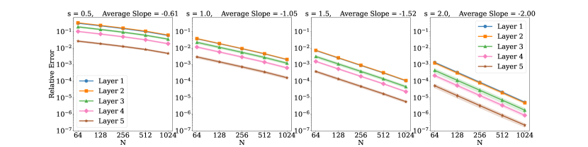
Figure 1: Relative error versus $N$ and $s$ for an FNO with default weight initialization.

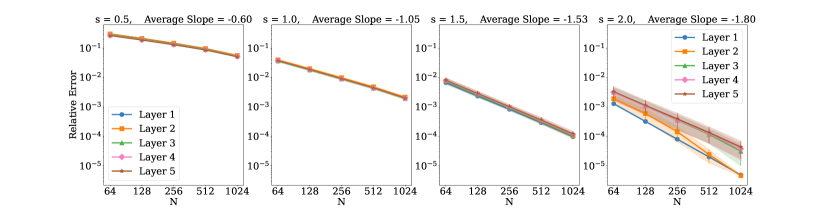
Figure 2: Relative error versus $N$ and $s$ for an FNO with default $\times 10$ initial weights.

4.1.1 Discretization Error

The relative error of the state at each layer versus the discretization for inputs of varying regularity may be seen for each of the five models in Figures 1, 2, 3, 4, and 5 respectively. In these figures, from left to right, $s\in\{0.5,1,1.5,2\}$ where $v_{0}\in H^{s-}$. The uncertainty shading indicates two standard deviations from the mean over five inputs to the FNO.

As can be seen in Figure 1 for the model with the default weight initialization, the empirical behavior of the error matches the behavior expected from Theorem 3.1. One question that arises from Figure 1 is why the error decreases as the number of layers increases; this is an effect of the magnitude of the weights. When the model weights are multiplied by $10$, then the error begins to increase with the number of layers, as can be seen in Figure 2. This phenomenon is also showcased in Figure 9(a) where the state norm remains the same order of magnitude through the layers for the default model but increases exponentially for the other three model initializations.

While the model behavior in the first two figures follows the theory, when all the weights are set equal to $1$ the behavior is more erratic; this can be seen in Figure 3. The error decreases faster than expected and with less consistency than the Gaussian weight models, and the decay rate increases with each layer. In this sense, the all-ones model has a smoothing effect on the state at each layer. We note that this generally occurs with any initialization that sets the spectral weights on the same order of magnitude as the affine weights; for instance, the same super-convergence effect occurs when all weights are initialized $U(0,1)$.

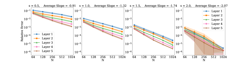
Figure 3: Relative error versus $N$ and $s$ for an FNO with all weights equals to $1$.

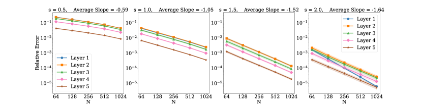
Figure 4: Relative error versus $N$ and $s$ for a default FNO with a ReLU activation.

The results shown in Figure 4 justify the use of the GeLU activation function, which belongs to $C^{\infty}$, over the ReLU activation function, which is only Lipschitz. The figure shows that the benefit of having sufficiently smooth inputs is negated by the ReLU activation: the error decay is limited. Note that this effect does not occur for the first layer since at that point ReLU has been applied once, and the Fourier transform is not applied to the output of an activation function until the second layer. Since the ReLU activation function has regularity of $s=1.5$, no improvement in convergence rate is observed when the inputs have higher regularity than this. Additionally, in the default model with $\times 10$ magnitude weights in Figure 2, the large weights mean that the GeLU activation acts like a ReLU activation for smaller discretizations. This phenomenon is apparent for inputs with regularity $s=2$, where the first layer has the appropriate slope, but the other layers only begin to approach that rate at higher discretizations. Earlier layers achieve this rate first because of the smaller magnitude state norm in earlier layers for this model.

A similar effect to the ReLU model occurs when positional encoding information is appended to the input; see Figure 5. Since this grid data has a jump discontinuity across the boundary of $[0,1]^{d}$, it has regularity of $s=0.5$, and the convergence rate is thus impacted.

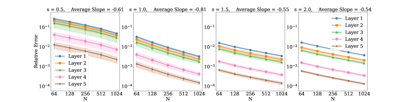
Figure 5: Relative error versus $N$ and $s$ for a default FNO with non-periodic position encoding appended to the input.

4.2 Experiments with Trained Networks

In this subsection, we consider two different maps and train FNOs on data from each map. Then we perform the same discretization error analysis as in Subsection 4.1. The first map is a PDE solution map in two dimensions whose solution is at least as regular as the input function. The second map is a simple gradient, but in this setting the output data of the gradient is, of course, less regular by one Sobolev smoothness exponent than that of the input function. In both experiments, periodic positional encoding information is appended to the inputs.

4.2.1 Discretization Error for PDE Solution Model

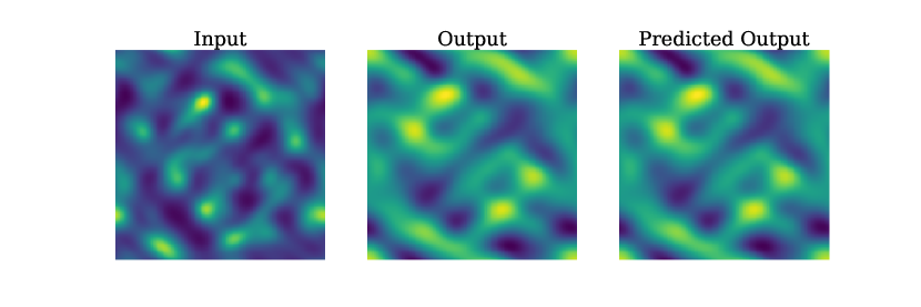
(a) Data for the PDE Solution FNO.

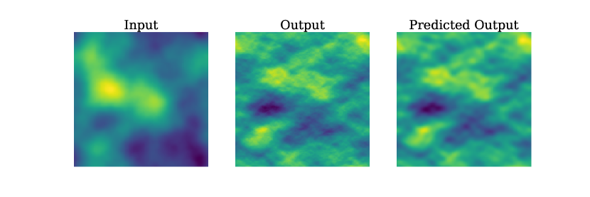
(b) Data for the Gradient FNO.

Figure 6: Visualization of the input and output data for the trained model examples.

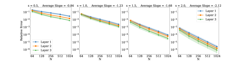
Figure 7: Error versus discretization for inputs of varying regularity for the FNO trained on data corresponding to a PDE solution.

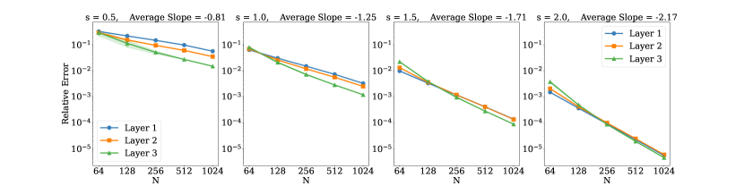
Figure 8: Error versus discretization for inputs of varying regularity for the FNO trained on data corresponding to a gradient map.

In this example, we train an FNO to approximate the solution map to the following PDE:

(4.2) $$\nabla\cdot(\nabla\chi A) =\nabla\cdot A,\quad y\in\mathbb{T}^{2}$$

(4.3) $$\chi\text{ is } 1-\text{periodic, }\int_{\mathbb{T}^{2}}\chi\;\mathsf{d}y=0.$$

Here, the input $A:\mathbb{T}^{2}\mapsto\mathbb{R}^{2\times 2}$ is symmetric positive definite at every point in the domain $\mathbb{T}^{2}$ and is bounded and coercive. For the output data we take the first component of $\chi:\mathbb{T}^{2}\mapsto\mathbb{R}^{2}$. In our experiments the model is trained to $<5\%$ relative $L^{2}$ test error. A visualization of the data is in Figure 6(a).

The error versus discretization analysis can be seen in Figure 7. The error decreases slightly faster than predicted by the theory; a potential explanation is that the trained model itself has a smoothing effect that is not exploited in our analysis.

4.2.2 Discretization Error for a Gradient Map

In the final example, we train an FNO to approximate a simple gradient map

(4.4) $$u\mapsto\nabla u.$$

The training data consists of iid Gaussian random field inputs with regularity $s=2$. Since a gradient reduces regularity, we expect the model outputs to approximate functions with regularity $s=1$, which is at odds with the smoothness-preserving properties of the FNO described by theory.

The error versus discretization for inputs of various smoothness is shown in Figure 8. The error decreases according the the smoothness of the input despite the smoothness-decreasing properties of the data. Indeed, the model does produce more regular predicted outputs than the true gradient, as can be seen in Figure 6(b) where the predicted output is visibly smoother than the true output.

4.3 Avoiding Discretization Error

The discretization error analyses performed in this section can be done on any FNO, trained or untrained. In practice, for a particular model size and input data regularity, these experiments may be done to calibrate which discretization level to use to achieve relative error from discretization at, or below, the order of magnitude of the desired test error of the model. Furthermore, to increase accuracy with discretization, the theory and experiments promote the use of periodic positional encodings instead of non-periodic encodings as well as the use of GeLU activation instead of ReLU. Finally, an additional potential application is adaptive subsampling, as described in the next subsection.

4.4 Speeding Up Training via Adaptive Subsampling

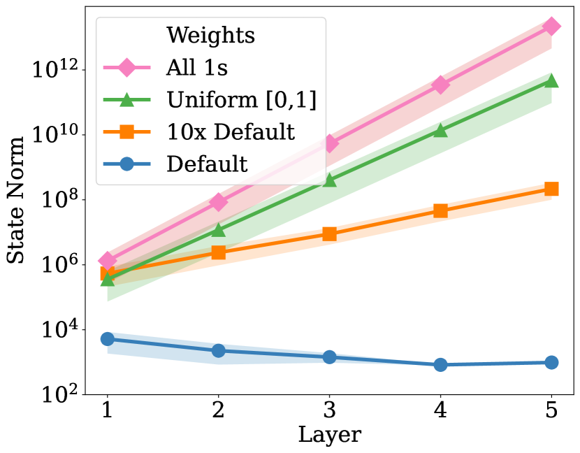
(a) State norm versus layer for various untrained model initializations.

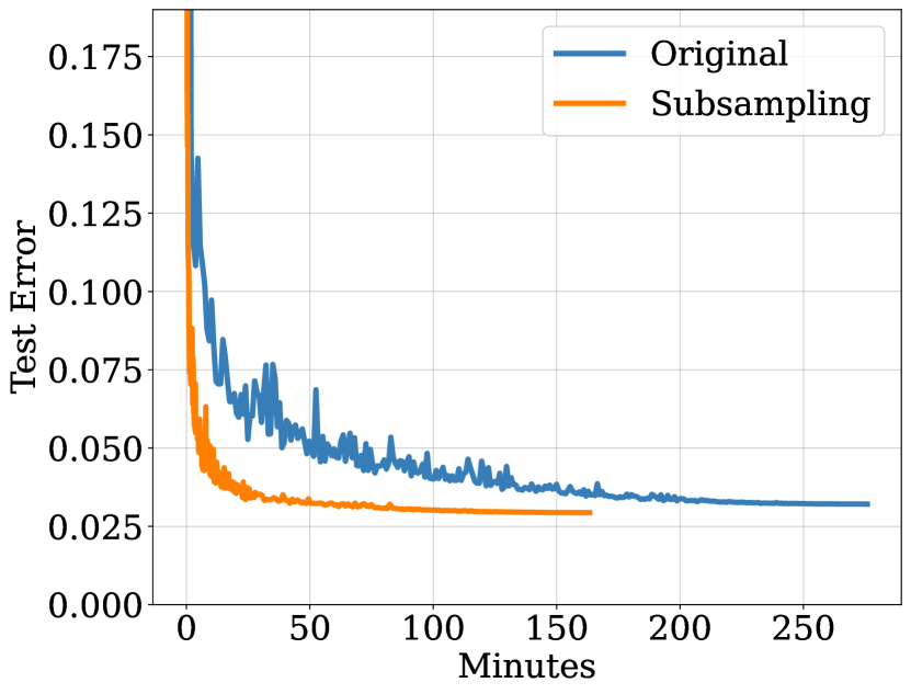
(b) Adaptive grid refinement leads to greater training efficiency.

Figure 9:

The fact that the FNO architecture and its parametrization are independent of the numerical discretization allows for increased flexibility. Specifically, it is possible to adaptively choose an optimal discretization for a given objective. We close this section by exploring one such possibility with the aim of optimizing computational time during training.

The overall approximation error of the FNO can be split into a contribution due to the numerical discretization and another contribution due to model discrepancy,

$$\Psi^{\dagger}-\Psi_{FNO}^{N}=\underbrace{\left[\Psi^{\dagger}-\Psi_{FNO}\right]}_{\text{model discrepancy}}+\underbrace{\left[\Psi_{FNO}-\Psi_{FNO}^{N}\right]}_{\text{discretization error}}.$$

Here, $\Psi^{\dagger}$ is the ground truth operator, $\Psi^{N}_{FNO}$ represents the discretized FNO with grid size $N$, and $\Psi_{FNO}$ represents the continuous FNO in the absence of discretization errors. The basic idea of our proposed approach is that, during training, it is not necessary to compute model outputs to a numerical accuracy that is substantially better than the model discrepancy. This suggests an adaptive choice of the numerical discretization, where we employ a coarser grid during the early phase of training and refine the grid in later stages. In practice, we realize this idea by introducing a subsampling scheduler. The subsampling scheduler tracks a validation error on held out data, and adaptively changes the numerical resolution via suitable subsampling of the training data. Starting from a coarse resolution, we iteratively double the grid size once the validation error plateaus.

We train FNO for the elliptic PDE (4.2) with and without the subsampling scheduler. Our model has 4 hidden layers, channel width 64 and Fourier cut-off 12. Our results are based on 9000 training samples and 500 test samples. For training with a subsampling scheduler, we include an additional 500 samples for validation. Compared to training without subsampling, training with a subsampling scheduler therefore requires the same number of forward and backward passes over the network for the training and test set, plus an additional overhead due to the validation set. Since we are mainly interested in the training time, our choice of adding validation samples, rather than performing a training/validation split of the 9000 original samples, ensures that computational timings are not skewed in favor of subsampling. Over the course of training, we iterate through the following grid sizes: 32x32, 64x64, and 128x128. Our criterion for a plateau is that the validation error has not improved for 40 training epochs. Models are trained for 300 epochs on an Nvidida P100 GPU.

The results of training with and without subsampling scheduler for the PDE solution model (4.2) are shown in Figure 9(b). We observe that training time can be substantially reduced with subsampling. This points to the potential benefits of developing adaptive numerical methods for model evaluation within operator learning.

5 Conclusions

In this paper, we analyze the error that results from Fourier Neural Operators (FNOs) when implemented on a grid rather than on a continuum. We bound the $L^{2}$ norm of the error in Theorem 3.1, proving an upper bound that decreases asymptotically as $N^{-s}$, where $N$ is the discretization in each dimension, and $s$ is the input regularity. We show empirically that FNOs with random weights chosen as the default FNO weights for training behave almost exactly as the theory predicts. Furthermore, our theory and experiments justify the use of the GeLU activation function in FNO over ReLU, as the former preserves regularity. Additional analyses on trained models show that the error behaves less predictably in relation to our theory in the low-discretization regime. Finally, we provide basic guidelines for mitigating against discretization error in practical settings and propose an adaptive subsampling algorithm for decreasing training time with operator learning. As FNOs become a more common tool in scientific machine learning, understanding the various sources of error is critical. By bounding FNO discretization error and demonstrating its behavior in numerical experiments, we understand its effect on learning and the potential to minimize computational costs by an adaptive choice of numerical resolution.

Appendices

Appendix A Trigonometric Interpolation and Aliasing

In this section, we present a self-contained analysis of aliasing errors for $v\in H^{s}(\mathbb{T}^{d})$. The primary goal is to state and prove Proposition A.10, which controls the difference between a function defined over $\mathbb{T}^{d}$ and the trigonometric interpolation of a function defined on a grid. In the following, we denote by $N$ an integer. We recall that $X^{(N)}$ is a set of equidistant grid points on the torus $\mathbb{T}^{d}$,

$$X^{(N)}=\{x_{n}\in\mathbb{T}^{d}\,|\,x=n/N,\;n\in[N]^{d}\}.$$

We note that the discrete Fourier transform gives rise to a natural correspondence between grid values and Fourier modes,

(A.1) $$\{v(x_{n})\}_{n\in[N]^{d}}\;\leftrightarrow\;\{\tilde{c}_{k}\}_{k\in[[N]]^{d}},$$

where

(A.2) $$\tilde{c}_{k}=\frac{1}{N^{d}}\sum_{n\in[N]^{d}}v(x_{n})e^{-2\pi i\langle k,x_{n}\rangle}=:\mathsf{DFT}(v)(k).$$

We begin with the following observation:

Lemma A.1.

Let $N$ be given. Then,

(A.3) $$\frac{1}{N^{d}}\sum_{k\in[[N]]^{d}}e^{2\pi i\langle k,x_{m}-x_{n}\rangle}=\delta_{mn},\quad\forall\,m,n\in[N]^{d},$$

(A.4) $$\frac{1}{N^{d}}\sum_{n\in[N]^{d}}e^{2\pi i\langle k-k^{\prime},x_{n}\rangle}=\delta_{kk^{\prime}},\quad\forall\,k,k^{\prime}\in[[N]]^{d}.$$

Proof A.2.

This follows from an elementary calculation, which we briefly recall here. For $d=1$, the claim follows by noting that $x_{n}=n/N$, and using the identity

(A.5) $$\sum_{\ell=0}^{N-1}q^{\ell}=\begin{cases}\frac{q^{N}-1}{q-1},&(q\neq 1),\\ N,&(q=1),\end{cases}$$

with $q=e^{2\pi i(m-n)/N}$ and $q=e^{2\pi i(k-k^{\prime})/N}$, respectively. Indeed, assuming $d=1$ and denoting $-K:=\min[[N]]$, then the above identity implies, for example,

$$\sum_{k\in[[N]]}e^{2\pi ik(x_{m}-x_{n})}=\sum_{k\in[[N]]}\big{[}\underbrace{e^{2\pi i(m-n)/N}}_{=:q}\big{]}^{k}=\sum_{k\in[[N]]}q^{k}=q^{-K}\sum_{\ell=0}^{N-1}q^{\ell}.$$

If $q\neq 1$, then $q^{N}=e^{2\pi i(m-n)}=1$. By (A.5), this implies that the last sum is $0$. On the other hand, if $q=1$, then the last sum is trivially $=N$. We finally note that, for $m,n\in[N]$, we have $q=1$ if and only if $m=n$, implying that

$$q^{-K}\sum_{\ell=0}^{N}q^{\ell}=N\delta_{mn}.$$

Thus,

$$\sum_{k\in[[N]]}e^{2\pi ik(x_{m}-x_{n})}=N\delta_{mn},$$

and (A.3) follows. The argument for (A.4) is analogous. For $d>1$, the sum over $[[N]]^{d}=[[N]]\times\dots\times[[N]]$ is split into sums along each dimension, and the same argument is applied for each of the $d$ components, yielding the claim also for $d>1$.

A trigonometric polynomial $p:\mathbb{T}^{d}\mapsto\mathbb{R}^{m}$ is a function of the form

(A.6) $$p(x)=\sum_{k\in[[N]]^{d}}c_{k}e^{2\pi i\langle k,x\rangle}$$

with $c_{k}\in\mathbb{C}^{m}$ chosen to make $p(x)$ $\mathbb{R}^{m}$-valued at each $x\in\mathbb{T}^{d}.$ We note that the discrete and continuous $L^{2}$-norms are equivalent for trigonometric polynomials:

Lemma A.3.

Let $N$ be a positive integer. If $p(x)$ is a trigonometric polynomial, then

$$\frac{1}{N^{d/2}}\|p\|_{\ell^{2}(n\in[N]^{d})}=\|p\|_{L^{2}(\mathbb{T}^{d})}.$$

Proof A.4.

We have

$$\|p\|_{L^{2}(\mathbb{T}^{d})}^{2}=\int_{\mathbb{T}^{d}}|p(x)|^{2}\,dx=\sum_{k,k^{\prime}\in[[N]]^{d}}c_{k}\overline{c}_{k^{\prime}}\underbrace{\int_{\mathbb{T}^{d}}e^{2\pi i\langle k-k^{\prime},x\rangle}\,dx}_{=\delta_{kk^{\prime}}}=\sum_{k\in[[N]]^{d}}|c_{k}|^{2},$$

and

$$\frac{1}{N^{d}}\|p\|_{\ell^{2}(n\in[N]^{d})}^{2} =\frac{1}{N^{d}}\sum_{n\in[N]^{d}}|p(x_{n})|^{2}$$

$$=\sum_{k,k^{\prime}\in[[N]]^{d}}c_{k}\overline{c}_{k^{\prime}}\underbrace{\frac{1}{N^{d}}\sum_{n\in[N]^{d}}e^{2\pi i\langle k-k^{\prime},x_{n}\rangle}}_{=\delta_{kk^{\prime}}}$$

$$=\sum_{k\in[[N]]^{d}}|c_{k}|^{2}.$$

This proves the claim.

Let $v:\mathbb{T}^{d}\to\mathbb{R}$ be a function with grid values $\{v(x_{n})\}_{n\in[N]^{d}}$. Let $\mathsf{DFT}(v)(k)$ denote the coefficients of the discrete Fourier transform defined by (A.1). Then

(A.7) $$p(x):=\sum_{k\in[[N]]^{d}}\mathsf{DFT}(v)(k)e^{2\pi i\langle k,x\rangle},$$

is the trigonometric polynomial associated to $v$. The next lemma shows that $p(x)$ interpolates $v(x)$.

Lemma A.5.

The trigonometric polynomial $p(x)$ defined by (A.7) interpolates $v(x)$ at the grid points, i.e., we have $p(x_{n})=v(x_{n})$ for all $n\in[N]^{d}$.

Proof A.6.

Fix $n\in[N]^{d}$. Then

$$p(x_{n}) =\sum_{k\in[[N]]^{d}}\mathsf{DFT}(v)(k)e^{2\pi i\langle k,x_{n}\rangle}$$

$$=\sum_{k\in[[N]]^{d}}\left\{\frac{1}{N^{d}}\sum_{m\in[N]^{d}}v(x_{m})e^{-2\pi i\langle k,x_{m}\rangle}\right\}e^{2\pi i\langle k,x_{n}\rangle}$$

$$=\sum_{m\in[N]^{d}}v(x_{m})\left\{\frac{1}{N^{d}}\sum_{k\in[[N]]^{d}}e^{2\pi i\langle k,x_{n}-x_{m}\rangle}\right\}$$

$$=\sum_{m\in[N]^{d}}v(x_{m})\delta_{mn}$$

$$=v(x_{n}),$$

where we have made use of (A.3) to pass to the fourth line.

The following trigonometric polynomial interpolation estimate for functions in Sobolev spaces $H^{s}(\mathbb{T}^{d})$ will be useful in stating our main proposition:

Lemma A.7.

Let $v\in H^{s}(\mathbb{T}^{d})$ for $s>d/2$. Let $p$ denote the interpolating trigonometric polynomial given by (A.7). Then

(A.8) $$v(x)-p(x)=\sum_{k\in\mathbb{Z}^{d}\setminus[[N]]^{d}}\widehat{v}(k)e^{2\pi i\langle k,x\rangle}-\sum_{k\in[[N]]^{d}}\left\{\sum_{\ell\in\mathbb{Z}^{d}\setminus\{0\}}\widehat{v}(k+\ell N)\right\}e^{2\pi i\langle k,x\rangle}.$$

Furthermore, there exists a constant $c_{s,d}>0$, such that

(A.9) $$\|v-p\|_{L^{2}(\mathbb{T}^{d})}\leq c_{s,d}\|v\|_{H^{s}(\mathbb{T}^{d})}N^{-s}.$$

Remark A.8.

The first sum on the right-hand side of (A.8) is the $L^{2}$-orthogonal Fourier projection of $v$ onto the complement of $\mathrm{span}\{e^{2\pi i\langle k,x\rangle}\,|\,k\in[[N]]^{d}\}$. The second sum in (A.8) is an “aliasing” error; It arises because two Fourier modes are indistinguishable on the discrete grid whenever $k-k^{\prime}\in N\mathbb{Z}^{d}$, i.e. $e^{2\pi i\langle k,x_{n}\rangle}=e^{2\pi i\langle k^{\prime},x_{n}\rangle}$ for all $n\in[N]^{d}$.

Proof A.9.

Since $v\in H^{s}(\mathbb{T}^{d})$ has Sobolev smoothness $s$ for $s>d/2$, it can be shown that the Fourier series of $v$ is uniformly convergent, and the following manipulations can be rigorously justified: First, substitution of $v(x_{n})=\sum_{k^{\prime}\in\mathbb{Z}^{d}}\widehat{v}(k^{\prime})e^{2\pi i\langle k^{\prime},x_{n}\rangle}$ into $\mathsf{DFT}(v)(k)$ yields

$$\mathsf{DFT}(v)(k) =\frac{1}{N^{d}}\sum_{n\in[N]^{d}}\left\{\sum_{k^{\prime}\in\mathbb{Z}^{d}}\widehat{v}(k^{\prime})e^{2\pi i\langle k^{\prime},x_{n}\rangle}\right\}e^{-2\pi i\langle k,x_{n}\rangle}$$

$$=\sum_{k^{\prime}\in\mathbb{Z}^{d}}\widehat{v}(k^{\prime})\left\{\frac{1}{N^{d}}\sum_{n\in[N]^{d}}e^{2\pi i\langle k^{\prime}-k,x_{n}\rangle}\right\}$$

We now note that

$$\frac{1}{N^{d}}\sum_{n\in[N]^{d}}e^{2\pi i\langle k^{\prime}-k,x_{n}\rangle}=\begin{cases}0,&(k^{\prime}\not\equiv k\mod{N}),\\ 1,&(k^{\prime}\equiv k\mod{N}),\end{cases}$$

as a consequence of the trigonometric identity (A.4). Writing $k^{\prime}=k+\ell N$ for all $k^{\prime}$ for which the sum inside the braces does not vanish, it follows that

$$\mathsf{DFT}(v)(k)=\sum_{\ell\in\mathbb{Z}^{d}}\widehat{v}(k+\ell N).$$

Thus,

$$v(x)-p(x) =\sum_{k\in\mathbb{Z}^{d}}\widehat{v}(k)e^{2\pi i\langle k,x\rangle}-\sum_{k\in[[N]]^{d}}\mathsf{DFT}(v)(k)e^{2\pi i\langle k,x\rangle}$$

$$=\sum_{k\in\mathbb{Z}^{d}\setminus[[N]]^{d}}\widehat{v}(k)e^{2\pi i\langle k,x\rangle}+\sum_{k\in[[N]]^{d}}\left\{\widehat{v}(k)-\mathsf{DFT}(v)(k)\right\}e^{2\pi i\langle k,x\rangle}$$

$$=\sum_{k\in\mathbb{Z}^{d}\setminus[[N]]^{d}}\widehat{v}(k)e^{2\pi i\langle k,x\rangle}-\sum_{k\in[[N]]^{d}}\left\{\sum_{\ell\in\mathbb{Z}^{d}\setminus\{0\}}\widehat{v}(k+\ell N)\right\}e^{2\pi i\langle k,x\rangle}.$$

We proceed to bound the last two terms. For the first term, we have

$$\Big{\|}\sum_{k\in\mathbb{Z}^{d}\setminus[[N]]^{d}}\widehat{v}(k)e^{2\pi i\langle k,x\rangle}\Big{\|}_{L^{2}(\mathbb{T}^{d})}^{2} =\sum_{k\in\mathbb{Z}^{d}\setminus[[N]]^{d}}|\widehat{v}(k)|^{2}$$

$$\leq\frac{1}{(1+(N/2)^{2s})}\sum_{k\in\mathbb{Z}^{d}}(1+|k|^{2s})|\widehat{v}(k)|^{2}$$

$$\leq 4^{s}N^{-2s}\|v\|^{2}_{H^{s}(\mathbb{T}^{d})},$$

where $\|v\|^{2}_{H^{s}(\mathbb{T}^{d})}=\sum_{k\in\mathbb{Z}^{d}}(1+|k|^{2s})|\widehat{v}(k)|^{2}$, and for the second term

$$\Big{\|}\sum_{k\in[[N]]^{d}}\Big{\{}\sum_{\ell\in\mathbb{Z}^{d}\setminus\{0\}} \widehat{v}(k+\ell N)\Big{\}}e^{2\pi i\langle k,x\rangle}\Big{\|}_{L^{2}(\mathbb{T}^{d})}^{2}$$

$$=\sum_{k\in[[N]]^{d}}\Big{|}\sum_{\ell\in\mathbb{Z}^{d}\setminus\{0\}}\widehat{v}(k+\ell N)\Big{|}^{2}$$

$$\leq\sum_{k\in[[N]]^{d}}\Big{(}\sum_{\ell\in\mathbb{Z}^{d}\setminus\{0\}}(1+|k+\ell N|^{2s})^{-1}\Big{)}$$

$$\qquad\times\Big{(}\sum_{\ell\in\mathbb{Z}^{d}\setminus\{0\}}(1+|k+\ell N|^{2s})|\widehat{v}(k+\ell N)|^{2}\Big{)}.$$

We note that for $k\in[[N]]^{d}$, we have $|k|_{\infty}\leq N/2$, and hence, for any integer vector $\ell\neq 0$, we obtain

(A.10) $$|k+\ell N|\geq|k+\ell N|_{\infty}\geq|\ell|_{\infty}N-|k|_{\infty}\geq|\ell|_{\infty}N-\frac{N}{2}\geq\frac{N}{2}|\ell|_{\infty}\geq\frac{N}{2\sqrt{d}}|\ell|.$$

We can now bound

(A.11a) $$\sum_{\ell\in\mathbb{Z}^{d}\setminus\{0\}}(1+|k+\ell N|^{2s})^{-1} \leq\sum_{\ell\in\mathbb{Z}^{d}\setminus\{0\}}\left(\frac{N}{2\sqrt{d}}\right)^{-2s}|\ell|^{-2s}$$

(A.11b) $$\leq c_{d,s}N^{-2s},$$

where $c_{d,s}:=(4d)^{s}\sum_{\ell\in\mathbb{Z}^{d}\setminus\{0\}}|\ell|^{-2s}<\infty$ is finite, since $s>d/2$ implies that the last series converges. Substitution of this bound in the estimate above implies,

$$\Bigg{\|}\sum_{k\in[[N]]^{d}}\Big{\{}\sum_{\ell\in\mathbb{Z}^{d}\setminus\{0\}} \widehat{v}(k+\ell N)\Big{\}}e^{2\pi i\langle k,x\rangle}\Bigg{\|}_{L^{2}(\mathbb{T}^{d})}^{2}$$

$$\leq c_{d,s}N^{-2s}\sum_{k\in[[N]]^{d}}\left(\sum_{\ell\in\mathbb{Z}^{d}\setminus\{0\}}(1+|k+\ell N|^{2s})|\widehat{v}(k+\ell N)|^{2}\right)$$

$$\leq c_{d,s}N^{-2s}\|v\|_{H^{s}(\mathbb{T}^{d})}^{2}.$$

Combining the above estimates, we conclude that

$$\|v-p\|_{L^{2}}\leq c_{d,s}\|v\|_{H^{s}(\mathbb{T}^{d})}N^{-s},$$

where we have re-defined $c_{d,s}:=2^{s}+(4d)^{s/2}\sum_{\ell\in\mathbb{Z}^{d}\setminus\{0\}}|\ell|^{-2s}$.

We can now state the main outcome of this section:

Proposition A.10.

Let $v\in H^{s}(\mathbb{T}^{d})$ be given for $s>d/2$ and let $\{u^{N}(x_{n})\}_{n\in[N]^{d}}$ be any grid values. Let $p^{N}(x)=\sum_{k\in[[N]]^{d}}\mathsf{DFT}(u^{N})(k)e^{2\pi i\langle k,x\rangle}$ be the interpolating trigonometric polynomial of $u^{N}$. Then,

$$\|v-p^{N}\|_{L^{2}(\mathbb{T}^{d})}\leq\frac{1}{N^{d/2}}\|v-u^{N}\|_{\ell^{2}(n\in[N]^{d})}+c_{d,s}\|v\|_{H^{s}(\mathbb{T}^{d})}N^{-s}.$$

Proof A.11.

Let $p(x)=\sum_{k\in[[N]]^{d}}\mathsf{DFT}(v)(k)e^{2\pi i\langle k,x\rangle}$ be the interpolating trigonometric polynomial given the point-values $\{v(x_{n})\}_{n\in[N]^{d}}$. Then,

(A.12) $$\|v-p^{N}\|_{L^{2}(\mathbb{T}^{d})}\leq\|v-p\|_{L^{2}(\mathbb{T}^{d})}+\|p-p^{N}\|_{L^{2}(\mathbb{T}^{d})}.$$

By Lemma A.7, we have

$$\|v-p\|_{L^{2}(\mathbb{T}^{d})}\leq c_{d,s}\|v\|_{H^{s}}N^{-s}.$$

By Lemma A.3, and since $p(x_{n})=v(x_{n})$, $p^{N}(x_{n})=u^{N}(x_{n})$ by Lemma A.5, we have

$$\|p-p^{N}\|_{L^{2}(\mathbb{T}^{d})} =\frac{1}{N^{d/2}}\|p(x_{n})-p^{N}(x_{n})\|_{\ell^{2}(n\in[N]^{d})}$$

$$=\frac{1}{N^{d/2}}\|v(x_{n})-u^{N}(x_{n})\|_{\ell^{2}(n\in[N]^{d})}.$$

Substitution in (A.12) gives the claimed bound.

Appendix B Discretization Error Derivation

In this section, we derive the error breakdown within each FNO layer. This error breakdown is used in the proofs of subsequent sections.

Let $\mathcal{E}^{(0)}_{t}$ be the error in the inputs to FNO layer $t$ such that

$$\mathcal{E}^{(0)}_{t}(x_{n})=v^{N}_{t}(x_{n})-v_{t}(x_{n}),\quad x_{n}\in X^{(N)}.$$

Let $\mathcal{F}$ denote the Fourier transform and $\mathsf{DFT}$ as in equation (A.2). Then for $k\in[[K]]^{d},$

$$\mathsf{DFT}(v^{N}_{t})(k) =\frac{1}{N^{d}}\sum_{n\in[N]^{d}}v_{t}(x_{n})e^{-2\pi i\langle k,x_{n}\rangle}+\frac{1}{N^{d}}\sum_{n\in[N]^{d}}\mathcal{E}^{(0)}_{t}(x_{n})e^{-2\pi i\langle k,x_{n}\rangle}$$

$$=\mathcal{F}(v_{t})(k)+\mathcal{E}^{(1)}_{t}(k)+\mathcal{E}^{(2)}_{t}(k)$$

where $\mathcal{E}^{(1)}_{t}$ is the error resulting from computing the Fourier transform of $v_{t}$ on a discrete grid rather than all of $\mathbb{T}^{d}$, i.e.

$$\mathcal{E}_{t}^{(1)}(k)=\frac{1}{N^{d}}\sum_{n\in[N]^{d}}v_{t}(x_{n})e^{-2\pi i\langle k,x_{n}\rangle}-\int_{\mathbb{T}^{d}}v_{t}(x)e^{-2\pi i\langle k,x\rangle}\;\;\mathsf{d}x$$

and $\mathcal{E}^{(2)}_{t}$ is the error $\mathcal{E}^{(0)}_{t}$ after the discrete Fourier transform, i.e.

$$\mathcal{E}^{(2)}_{t}(k)=\frac{1}{N^{d}}\sum_{n\in[N]^{d}}\mathcal{E}^{(0)}_{t}(x_{n})e^{-2\pi i\langle k,x_{n}\rangle}.$$

For $x_{n}\in X^{(N)}$, the output of the kernel integral operator is given by

$$(\mathcal{K}_{t}v^{N}_{t})(x_{n}) =\sum_{k\in[[K]]^{d}}P_{t}^{(k)}\left(\mathcal{F}(v_{t})(k)+\mathcal{E}^{(1)}_{t}(k)+\mathcal{E}^{(2)}_{t}(k)\right)e^{2\pi i\langle k,x_{n}\rangle}$$

$$=(\mathcal{K}_{t}v_{t})(x_{n})+\mathcal{E}^{(3)}_{t}(x_{n})$$

where

$$\mathcal{E}^{(3)}_{t}(x_{n})=\sum_{k\in[[K]]^{d}}P_{t}^{(k)}\left(\mathcal{E}^{(1)}(k)+\mathcal{E}^{(2)}(k)\right)e^{2\pi i\langle k,x_{n}\rangle}.$$

Finally, the output of layer $t$ is given by

$$v^{N}_{t+1}(x_{n}) =\sigma\left(W_{t}\bigl{(}v_{t}(x_{n})+\mathcal{E}^{(0)}_{t}(x_{n})\bigr{)}+(\mathcal{K}_{t}v^{N}_{t})(x_{n})+b_{t}\right)$$

$$=\sigma\left(W_{t}v_{t}(x_{n})+\mathcal{K}_{t}v_{t}(x_{n})+b_{t}+W_{t}\mathcal{E}^{(0)}_{t}(x_{n})+\mathcal{E}^{(3)}_{t}(x_{n})\right).$$

Therefore, the initial error for the next layer is given by

$$\mathcal{E}^{(0)}_{t+1}(x_{n}) =\sigma\left(W_{t}v_{t}(x_{n})+\mathcal{K}_{t}v_{t}(x_{n})+b_{t}+W_{t}\mathcal{E}^{(0)}_{t}(x_{n})+\mathcal{E}^{(3)}_{t}(x_{n})\right)$$

$$-\sigma\left(W_{t}v_{t}(x_{n})+\mathcal{K}_{t}v_{t}(x_{n})+b_{t}\right).$$

Appendix C Proofs of Approximation Theory Lemmas

The proof of Lemma 3.4 involves bounds on the error components described in Appendix B. We bound these components in the following proposition.

Proposition C.1.

Under Assumptions 3, it holds that

1. $\|\mathcal{E}^{(1)}_{t}\|_{\ell^{2}(k\in[[K]]^{d})}\leq\alpha_{d,s}N^{-s}\|v_{t}\|_{H^{s}}$ where $\alpha_{d,s}$ is independent of $N,v_{t}$;

2. $\|\mathcal{E}^{(2)}_{t}\|_{\ell^{2}(k\in[[N]]^{d})}=N^{-d/2}\|\mathcal{E}^{(0)}_{t}\|_{\ell^{2}(n\in[N]^{d})}$;

3. $\|\mathcal{E}^{(3)}_{t}\|_{\ell^{2}(n\in[N]^{d})}\leq N^{d/2}\|P_{t}\|_{F}\left(\|\mathcal{E}^{(1)}_{t}\|_{\ell^{2}(k\in[[K]]^{d})}+\|\mathcal{E}^{(2)}_{t}\|_{\ell^{2}(k\in[[K]]^{d})}\right);$

4. $\|\mathcal{E}^{(0)}_{t+1}\|_{\ell^{2}(n\in[N]^{d})}\leq B\left(\|W_{t}\|_{2}\|\mathcal{E}^{(0)}_{t}\|_{\ell^{2}(n\in[N]^{d})}+\|\mathcal{E}^{(3)}_{t}\|_{\ell^{2}(n\in[N]^{d})}\right)$.

Proof C.2.

Beginning with the definition of $\mathcal{E}^{(1)}_{t}(k)$, we have

$$\|\mathcal{E}^{(1)}_{t}\|_{\ell^{2}(k\in[[K]]^{d})}^{2} =\Big{\|}\frac{1}{N^{d}}\sum_{n\in[N]^{d}}v_{t}(x_{n})e^{-2\pi i\langle k,x_{n}\rangle}-\int_{\mathbb{T}^{d}}e^{-2\pi i\langle k,x\rangle}v_{t}(x)\;\mathsf{d}x\Big{\|}_{\ell^{2}(k\in[[K]]^{d})}^{2}.$$

Denote the terms in the above expression $\widehat{v}_{t}(k)$ and $\widehat{v}^{\dagger}_{t}(k)$, respectively. Since $s>\frac{d}{2}$,

$$v_{t}(x_{n})=\sum_{k\in\mathbb{Z}^{d}}\widehat{v}^{\dagger}_{t}(k)e^{2\pi i\langle k,x_{n}\rangle},$$

and it follows that

$$\widehat{v}_{t}(k^{\prime}) =\frac{1}{N^{d}}\sum_{n\in[N]^{d}}\left(\sum_{k\in\mathbb{Z}^{d}}\widehat{v}^{\dagger}_{t}(k)e^{2\pi i\langle k,x_{n}\rangle}\right)e^{-2\pi i\langle k^{\prime},x_{n}\rangle}$$

$$=\sum_{k\in\mathbb{Z}^{d}}\widehat{v}^{\dagger}_{t}(k)\frac{1}{N^{d}}\sum_{n\in[N]^{d}}e^{2\pi i\langle k-k^{\prime},x_{n}\rangle}$$

$$=\sum_{\ell\in\mathbb{Z}^{d}}\widehat{v}^{\dagger}_{t}(k^{\prime}+N\ell).$$

Therefore,

$$\|\mathcal{E}^{(1)}_{t} \|_{\ell^{2}(k\in[[K]]^{d})}^{2}=\|\widehat{v}_{t}-\widehat{v}^{\dagger}_{t}\|^{2}_{\ell^{2}(k\in[[K]]^{d})}$$

$$=\sum_{k\in[[K]]^{d}}\left|\sum_{\ell\in\mathbb{Z}^{d}\setminus\{0\}}\widehat{v}^{\dagger}_{t}(k+N\ell)\right|^{2}$$

$$\leq\sum_{k\in[[K]]^{d}}\left(\sum_{\ell\in\mathbb{Z}^{d}\setminus\{0\}}\frac{1}{|k+\ell N|^{2s}}\right)\sum_{\ell\in\mathbb{Z}^{d}\setminus\{0\}}|k+N\ell|^{2s}|\widehat{v}^{\dagger}_{t}(k+N\ell)|^{2}$$

We bound each component separately. It is clear from Definition 2.1 that

(C.1) $$\sum_{k\in[[K]]^{d}}\sum_{\ell\in\mathbb{Z}^{d}\setminus\{0\}}|k+N\ell|^{2s}|\widehat{v}^{\dagger}_{t}(k+N\ell)|^{2}\leq\|v_{t}\|_{H^{s}}^{2}.$$

To bound the first component independently of $k$, we note from $K<\frac{N}{2}$ and equation (A.10) that

$$\sum_{\ell\in\mathbb{Z}^{d}\setminus\{0\}}\frac{1}{|k+\ell N|^{2s}} \leq\sum_{\ell\in\mathbb{Z}^{d}\setminus\{0\}}\left(\frac{N}{2\sqrt{d}}|\ell|\right)^{-2s}$$

$$\leq\alpha_{d,s}^{2}N^{-2s}$$

by equation (A.11), where $\alpha^{2}_{d,s}=(4d)^{s}\sum_{\ell\in\mathbb{Z}^{d}\setminus\{0\}}|\ell|^{-2s}$ is finite since $s\geq\frac{d}{2}$. We express the final bound as

$$\|\mathcal{E}^{(1)}_{t}\|_{k\in[[K]]^{d}}\leq\alpha_{d,s}N^{-s}\|v_{t}\|_{H^{s}}.$$

For $\mathcal{E}^{(2)}_{t}(k)$ we have the definition

$$\mathcal{E}^{(2)}_{t}(k)=\frac{1}{N^{d}}\sum_{n\in[N]^{d}}\mathcal{E}^{(0)}_{t}(x_{n})e^{-2\pi i\langle k,x_{n}\rangle}.$$

By Parseval’s Theorem, we have

(C.2) $$\|\mathcal{E}^{(2)}_{t}\|^{2}_{\ell^{2}(k\in[[N]]^{d})}=\frac{1}{N^{d}}\|\mathcal{E}^{(0)}_{t}\|^{2}_{\ell^{2}(n\in[N]^{d})}.$$

For $P_{t}\in\mathbb{R}^{d_{v_{t+1}}\times K^{d}\times d_{v_{t}}}$ we define the tensor Frobenius norm
$\|P_{t}\|^{2}_{F}=\sum_{k\in[[K]]^{d}}\|P_{t}^{(k)}\|_{F}^{2}$.

$$\|\mathcal{E}^{(3)}_{t}\|_{\ell^{2}(n\in[N]^{d})}^{2} =\sum_{n\in[N]^{d}}\left|\sum_{k\in[[K]]^{d}}\ P_{t}^{(k)}\left(\mathcal{E}^{(1)}_{t}(k)+\mathcal{E}^{(2)}_{t}(k)\right)e^{2\pi i\langle k,x_{n}\rangle}\right|^{2}$$

$$\leq N^{d}\left|\sum_{k\in[[K]]^{2}}|P_{t}^{(k)}(\mathcal{E}^{(1)}_{t}(k)+\mathcal{E}^{(2)}_{t}(k))|\right|^{2}$$

$$\leq N^{d}\sum_{k\in[[K]]^{d}}\|P_{t}^{(k)}\|_{F}^{2}\sum_{k\in[[K]]^{d}}|\mathcal{E}^{(1)}_{t}(k)+\mathcal{E}^{(2)}_{t}(k)|^{2}$$

$$=N^{d}\|P_{t}\|_{F}^{2}\|\mathcal{E}^{(1)}_{t}+\mathcal{E}^{(2)}_{t}\|^{2}_{\ell^{2}(k\in[[K]]^{d})}$$

$$\|\mathcal{E}^{(3)}_{t}\|_{\ell^{2}(n\in[N]^{d})} \leq N^{d/2}\|P_{t}\|_{F}\left(\|\mathcal{E}^{(1)}_{t}\|_{\ell^{2}(k\in[[K]]^{d})}+\|\mathcal{E}^{(2)}_{t}\|_{\ell^{2}(k\in[[K]]^{d})}\right)$$

Finally, we have the definition

$$\|\mathcal{E}^{(0)}_{t+1}\|_{\ell^{2}(n\in[N]^{d})}^{2} =\sum_{n\in[N]^{d}}\left|\sigma(W_{t}v_{t}+\mathcal{K}_{t}v_{t}+b_{t}+W_{t}\mathcal{E}^{(0)}_{t}(x_{n})+\mathcal{E}^{(3)}_{t}(x_{n}))-\sigma(W_{t}v_{t}+\mathcal{K}_{t}v_{t}+b_{t})\right|^{2}$$

$$\leq\sum_{n\in[N]^{d}}B^{2}\left|W_{t}\mathcal{E}^{(0)}_{t}(x_{n})+\mathcal{E}^{(3)}_{t}(x_{n})\right|^{2}$$

$$\|\mathcal{E}^{(0)}_{t+1}\|_{\ell^{2}(n\in[N]^{d})} \leq B\left(\|W_{t}\|_{2}\|\mathcal{E}^{(0)}_{t}\|_{\ell^{2}(n\in[N]^{d})}+\|\mathcal{E}^{(3)}_{t}\|_{\ell^{2}(n\in[N]^{d})}\right)$$

where $\|\cdot\|_{2}$ is the matrix-$2$ norm.

The results of Proposition C.1 allow us to easily prove the following lemma. See 3.4

Proof C.3.

From Proposition C.1, and shortening the notation $\ell^{2}(n\in[N]^{d})$ to $\ell^{2}$,

$$\|\mathcal{E}^{(0)}_{t+1}\|_{\ell^{2}} \leq B\left(\|W_{t}\|_{2}\|\mathcal{E}^{(0)}_{t}\|_{\ell^{2}}+N^{d/2}\|P_{t}\|_{F}\left(\alpha_{d,s}N^{-s}\|v_{t}\|_{H^{s}}+N^{-d/2}\|\mathcal{E}^{(0)}_{t}\|_{\ell^{2}}\right)\right)$$

Combining terms gives

(C.3) $$\|\mathcal{E}^{(0)}_{t+1}\|_{\ell^{2}}\leq B\left(\big{(}\|W_{t}\|_{2}+\|P_{t}\|_{F}\big{)}\|\mathcal{E}^{(0)}_{t}\|_{\ell^{2}}+\alpha_{d,s}N^{d/2-s}\|P_{t}\|_{F}\|v_{t}\|_{H^{s}}\right).$$

Replacing $\|W_{t}\|_{2}$ and $\|P_{t}\|$ with $M$ and rescaling gives

$$\frac{1}{N^{d/2}}\|\mathcal{E}^{(0)}_{t+1}\|_{\ell^{2}(n\in[N]^{d})}\leq BM\left(\frac{2}{N^{d/2}}\|\mathcal{E}^{(0)}_{t}\|_{\ell^{2}(n\in[N]^{d})}+\alpha_{d,s}N^{-s}\|v_{t}\|_{H^{s}}\right).$$

Appendix D Proofs of Regularity Theory Lemmas

The proof of Lemma 3.7 relies on another result for bounding the $H^{s}$ norm of compositions of functions, which is largely taken from the lemma on page 273 of Section 2 in [19] without assuming an $L^{\infty}$ norm of $v$ less than $1$. We state a proof here for completeness.

Lemma D.1.

Assume $\varphi:\mathbb{T}^{d}\to\mathbb{T}^{d}$ possesses continuous derivatives up to order $r$ which are bounded by $B$. Then

$$|\varphi\circ v|_{r}\leq Bc\left(1+\|v\|_{\infty}^{r-1}\right)\|v\|_{H^{r}}$$

provided $v\in H^{r}(\mathbb{T}^{d})$, where $c$ is a constant dependent on $r$ and $d$.

Proof D.2.

By Faà di Bruno’s formula, we have

(D.1) $$D_{x}^{r}(\varphi\circ v(x))=\sum C_{\alpha,r}\frac{d^{\rho}\varphi}{dx^{\rho}}(v(x))\prod_{j=1}^{r}(D_{x}^{j}v(x))^{\alpha_{j}}$$

where the sum is over all nonnegative integers $\alpha_{1},\dots,\alpha_{r}$ such that $\alpha_{1}+2\alpha_{2}+\dots+r\alpha_{r}=r$, the constant $C_{\alpha,r}=\frac{r!}{\alpha_{1}!\alpha_{2}!2!^{\alpha_{2}}\dots\alpha_{r}!r!^{\alpha_{r}}}$, and $\rho:=\alpha_{1}+\alpha_{2}+\dots+\alpha_{r}$.

We seek a bound on square integrals of (D.1). Setting $v_{0}=\frac{d^{\rho}\varphi}{dx^{\rho}}v$, $v_{\lambda}=D_{x}^{\lambda}v$, $\alpha_{0}=1$, $p_{0}=\infty$, and $p_{\lambda}=\frac{r}{\lambda\alpha_{\lambda}}$ and noting that $\sum_{\lambda=0}^{r}\frac{1}{2p_{\lambda}}=\frac{1}{2}$, we have by Hölder’s inequality for multiple products that

$$\int_{\mathbb{T}^{d}}\left|\frac{d^{\rho}\varphi}{dx^{\rho}}(v(x))\prod_{j=1}^{r}(D_{x}^{j}v(x))^{\alpha_{j}}\right|^{2}\;\mathsf{d}x\leq\int_{\mathbb{T}^{d}}\prod_{\lambda=0}^{r}|v_{\lambda}|^{2\alpha_{\lambda}}\;\mathsf{d}x \leq\prod_{\lambda=0}^{r}\left(\int_{\mathbb{T}^{d}}|v_{\lambda}|^{2\alpha_{\lambda}p_{\lambda}}\;\mathsf{d}x\right)^{1/{p_{\lambda}}}$$

$$=\|v_{0}\|_{\infty}^{2}\prod_{\lambda=1}^{r}\left(\int_{\mathbb{T}^{d}}|v_{\lambda}|^{2\alpha_{\lambda}p_{\lambda}}\;\mathsf{d}x\right)^{1/{p_{\lambda}}}$$

The first factor is bounded above by $B^{2}$ by assumption. By application of Gagliardo-Nirenberg, the second factor may be bounded by

$$\prod_{\lambda=1}^{r}\left(\int_{\mathbb{T}^{d}}|D_{x}^{\lambda}v|^{2r/\lambda}\;\mathsf{d}x\right)^{\lambda\alpha_{\lambda}/r} \leq C^{r}\prod_{\lambda=1}^{r}\|v\|_{\infty}^{2\alpha_{\lambda}(1-\lambda/r)}\left(\|D_{x}^{r}v\|^{2}+\|v\|^{2}\right)^{\alpha_{\lambda}\lambda/r}$$

$$\leq C^{r}\|v\|_{\infty}^{2\rho-2}\|v\|_{H^{r}}^{2}$$

since $\sum_{\lambda}\lambda\alpha_{\lambda}=r$, and $\sum_{\lambda}\alpha_{\lambda}=\rho$. Combining the bounds,

$$\int_{\mathbb{T}^{d}}\prod_{\lambda=0}^{r}|v_{\lambda}|^{2\alpha_{\lambda}}\;\mathsf{d}x\leq B^{2}C^{r}\|v\|_{\infty}^{2\rho-2}\|v\|_{H^{r}}^{2}.$$

If $\|v\|_{\infty}<1$, we have the bound

(D.2) $$\int_{\mathbb{T}^{d}}\prod_{\lambda=0}^{r}|v_{\lambda}|^{2\alpha_{\lambda}}\;\mathsf{d}x\leq B^{2}C^{r}\|v\|_{H^{r}}^{2},$$

and otherwise since $\rho\leq r$,

(D.3) $$\int_{\mathbb{T}^{d}}\prod_{\lambda=0}^{r}|v_{\lambda}|^{2\alpha_{\lambda}}\;\mathsf{d}x\leq B^{2}C^{r}\|v\|_{\infty}^{2r-2}\|v\|^{2}_{H^{r}}.$$

Since these bounds hold for any term in the sum D.1, we obtain

(D.4) $$|\varphi\circ v|_{r}\leq Bc\left(1+\|v\|_{\infty}^{r-1}\right)\|v\|_{H^{r}}$$

for a different constant $c$ depending on $r$ and $d$.

Now we may prove Lemma 3.7. See 3.7

Proof D.3.

First we bound $\|\mathcal{K}_{t}v_{t}\|_{\infty}$ under the assumption that the Fourier transform is computed exactly (i.e. not on a grid). Let $\widehat{v}_{t}^{\dagger}(k):=\int_{\mathbb{T}^{d}}v_{t}(x)e^{-2\pi i\langle k,x\rangle}\;\mathsf{d}x$.

$$\|\mathcal{K}_{t}v_{t}\|_{\infty} =\|\sum_{k\in[[K]]^{d}}P^{(k)}_{t}\widehat{v}^{\dagger}_{t}(k)e^{2\pi i\langle k,x\rangle}\|_{\infty}$$

$$\leq\|P_{t}\|_{F}\sum_{k\in[[K]]^{d}}|\widehat{v}^{\dagger}_{t}(k)|$$

$$\leq\|P_{t}\|_{F}K^{d/2}\|\widehat{v}^{\dagger}_{t}(k)\|_{\ell^{2}(k\in[[K]]^{d})}$$

$$\leq\|P_{t}\|_{F}K^{d/2}\|v_{t}\|_{L^{2}(\mathbb{T}^{d})}.$$

Then

$$\|W_{t}v_{t}+\mathcal{K}_{t}v_{t}+b_{t}\|_{\infty}\leq\|W_{t}\|_{2}\|v_{t}\|_{\infty}+|b_{t}|+\|P_{t}\|_{F}K^{d/2}\|v_{t}\|_{L^{2}(\mathbb{T}^{d})},$$

and by Lipschitzness of $\sigma$ we have

$$\|v_{t+1}\|_{\infty}\leq\sigma_{0}+BM\left(1+\|v_{t}\|_{\infty}+K^{d/2}\|v_{t}\|_{L^{2}(\mathbb{T}^{d})}\right).$$

Next we bound $|v_{t+1}|_{s}$. Letting $f_{t}=W_{t}v_{t}+\mathcal{K}_{t}v_{t}+b_{t}$, we see from Lemma D.1 that bounding $\|f_{t}\|_{H^{s}}$ will give the result.

$$D_{x}^{s}(f_{t}) =W_{t}(D_{x}^{s}v_{t})+\mathcal{K}_{t}(D^{s}_{x}v_{t}).$$

$$\int_{\mathbb{T}^{d}}|D^{s}_{x}(f_{t})|^{2}\;\mathsf{d}x \leq 2\left(\int_{\mathbb{T}^{d}}|W_{t}(D^{s}_{x}v_{t})|^{2}\;\mathsf{d}x+\int_{\mathbb{T}^{d}}|\mathcal{K}_{t}(D^{s}_{x}v_{t})|^{2}\;\mathsf{d}x\right)$$

The first integral on the right may be bounded by $\|W_{t}\|_{2}^{2}|v_{t}|_{s}^{2}$. To bound the second integral,

$$\int_{\mathbb{T}^{d}}|\mathcal{K}_{t}(D^{s}_{x}v_{t})|^{2}\;\mathsf{d}x =\int_{\mathbb{T}^{d}}\left|\sum_{k\in[[K]]^{d}}P_{t}^{(k)}\widehat{g}_{t}^{\dagger}(k)e^{2\pi i\langle k,x\rangle}\right|^{2}\;\mathsf{d}x$$

where $\widehat{g}_{t}^{\dagger}(k)$ are the Fourier coefficients of $D^{s}_{x}v_{t}$. Continuing,

$$\int_{\mathbb{T}^{d}}|\mathcal{K}_{t}(D^{s}_{x}v_{t})|^{2}\;\mathsf{d}x \leq K^{d}\int_{\mathbb{T}^{d}}\|P_{t}\|^{2}\sum_{k\in[[K]]^{d}}|\widehat{g}_{t}^{\dagger}(k)|^{2}\;\mathsf{d}x$$

$$\leq\|P_{t}\|_{F}^{2}\|D^{s}_{x}v_{t}\|_{L^{2}}^{2},$$

giving a bound of

$$|f_{t}|_{s}\leq 2M|v_{t}|_{s}$$

In the following, $\lesssim$ denotes inequality up to a constant multiple that does not depend on any of the variables involved. Combining Lemma D.1 and the above bounds, we have

$$|\sigma\circ f_{t}|_{s} \leq Bc(1+\|f_{t}\|_{\infty}^{s-1})\|f_{t}\|_{H^{s}}$$

$$\leq Bc(1+(M(1+\|v_{t}\|_{\infty}+K^{d/2}\|v_{t}\|_{\infty}))^{s-1})(M(1+\|v_{t}\|_{\infty}+K^{d/2}\|v_{t}\|_{\infty})+2M|v_{t}|_{s})$$

$$\lesssim BcM^{s}K^{ds/2}(1+(1+\|v_{t}\|_{\infty})^{s-1})(1+\|v_{t}\|_{\infty}+|v_{t}|_{s})$$

$$\lesssim BcM^{s}K^{ds/2}(1+\|v_{t}\|_{\infty})^{s-1}(1+\|v_{t}\|_{\infty})(1+|v_{t}|_{s})$$

$$\lesssim BcM^{s}K^{ds/2}(1+\|v_{t}\|_{\infty})^{s}(1+|v_{t}|_{s}).$$

Appendix E Proof of Theorem 3.1

See 3.1

Proof E.1.

From Lemma 3.7 we have for $t\geq 1$,

$$\|v_{t}\|_{\infty} \lesssim\sigma_{0}\sum_{j=0}^{t-1}(BMK^{d/2})^{j}+\sum_{j=1}^{t}(BMK^{d/2})^{j}+(BMK^{d/2})^{t}\|v_{0}\|_{\infty}$$

$$|v_{t}|_{s} \lesssim\left(\sum_{j=1}^{t}(BcM^{s}K^{ds/2})^{j}\prod_{\ell=t-j}^{t-1}(1+\|v_{\ell}\|_{\infty})^{s}\right)+(BcM^{s}K^{ds/2})^{t}\left(\prod_{\ell=0}^{t-1}(1+\|v_{\ell}\|_{\infty})^{s}\right)|v_{0}|_{s}.$$

Denote $\max\{BMK^{d/2},B^{1/s}c^{1/s}MK^{d/2},1\}$ by $C_{0}$. The bound on $\|v_{t}\|_{\infty}$ simplifies to

$$\|v_{t}\|_{\infty} \lesssim\sigma_{0}\sum_{j=1}^{t}C_{0}^{j}+C_{0}^{t}\|v_{0}\|_{\infty}$$

$$\leq\sigma_{0}tC_{0}^{t}+C_{0}^{t}\|v_{0}\|_{\infty}$$

Plugging in this bound to the product in the bound on $|v_{t}|_{s}$, we have

$$\prod_{\ell=t-j}^{t-1}(1+\|v_{\ell}\|_{\infty})^{s} \lesssim\prod_{\ell=t-j}^{t-1}(\ell\sigma_{0}C_{0}^{\ell}+C_{0}^{\ell}\|v_{0}\|_{\infty})^{s}$$

$$\leq C_{0}^{tsj}(t)^{sj}(\sigma_{0}+\|v_{0}\|_{\infty})^{sj}.$$

Combining these two bounds, we attain the following bound on $|v_{t}|_{s}$ for $t\geq 1$.

$$|v_{t}|_{s} \lesssim\left(\sum_{j=1}^{t}(C_{0})^{sj}C_{0}^{tsj}(t)^{sj}(\sigma_{0}+\|v_{0}\|_{\infty})^{sj}\right)+C_{0}^{ts}\left(C_{0}^{t^{2}s}(t)^{st}(\sigma_{0}+\|v_{0}\|_{\infty})^{st}\right)|v_{0}|_{s}$$

$$\lesssim\left(\sum_{j=1}^{t}C_{0}^{2tsj}(t)^{sj}(\sigma_{0}+\|v_{0}\|_{\infty})^{sj}\right)+C_{0}^{2t^{2}s}(t)^{st}(\sigma_{0}+\|v_{0}\|_{\infty})^{st}|v_{0}|_{s}$$

$$\lesssim(C_{0}^{2t^{2}s}t^{st+1}+C_{0}^{2t^{2}s}t^{st}|v_{0}|_{s})(\sigma_{0}+\|v_{0}\|_{\infty})^{st}$$

and the following bound on $\|v_{t}\|_{H^{s}}$

(E.1) $$\|v_{t}\|_{H^{s}}\lesssim(C_{0}^{2t^{2}s}t^{st+1}|v_{0}|_{s})(\sigma_{0}+\|v_{0}\|_{\infty})^{st}+\sigma_{0}tC_{0}^{t}+C_{0}^{t}\|v_{0}\|_{\infty}.$$

Denote this upper bound by $C_{1}$, which does not depend on $N$. From Lemma 3.4, we have

$$\frac{1}{N^{d/2}}\|\mathcal{E}^{(0)}_{t+1}\|_{\ell^{2}(n\in[N]^{d})}\lesssim BM\left(\frac{2}{N^{d/2}}\|\mathcal{E}^{(0)}_{t}\|_{\ell^{2}(n\in[N]^{d})}+\alpha_{d,s}N^{-s}C_{1}\right).$$

By the discrete Gronwall lemma,

$$\frac{1}{N^{d/2}}\|\mathcal{E}^{(0)}_{t}\|_{\ell^{2}(n\in[N]^{d})} \lesssim\frac{BM\alpha_{d,s}N^{-s}C_{1}}{1-2BM}(1-(2BM)^{t})+\frac{1}{N^{d/2}}\|\mathcal{E}^{(0)}_{0}\|_{\ell^{2}(n\in[N]^{d})}(2BM)^{t}.$$

Since we assume we begin with no error, $\|\mathcal{E}^{(0)}_{0}\|_{\ell^{2}(n\in[N]^{d})}=0$, this simplifies to

$$\frac{1}{N^{d/2}}\|\mathcal{E}^{(0)}_{t}\|_{\ell^{2}(n\in[N]^{d})} \lesssim\frac{BM\alpha_{d,s}C_{1}}{1-2BM}(1-(2BM)^{t})N^{-s}.$$

Denoting the factor in front of $N^{-s}$ by $C$ and absorbing the effects of $\lesssim$ into $C$, we have the result that

$$\frac{1}{N^{d/2}}\|v_{t}-v_{t}^{N}\|_{\ell^{2}(n\in[N]^{d})}\leq CN^{-s}.$$

Appendix F Proof of Theorem 3.3

See 3.3

Proof F.1.

Let $p^{N}_{t}(x)$ be the interpolating trigonometric polynomial associated with the data $\{v^{N}_{t}(x_{n})\}_{n\in[N]^{d}}$. By Proposition A.10, we have

$$\|v_{t}-p^{N}_{t}\|_{L^{2}(\mathbb{T}^{d})}\leq\frac{1}{N^{d/2}}\|v_{t}-v^{N}_{t}\|_{\ell^{2}(n\in[N]^{d})}+c_{d,s}\|v\|_{H^{s}(\mathbb{T}^{d})}N^{-s}.$$

By (E.1), we have $\|v\|_{H^{s}(\mathbb{T}^{d})}\leq C_{1}$. Furthermore, it follows from Theorem 3.1, that

$$\frac{1}{N^{d/2}}\|v_{t}-v^{N}_{t}\|_{\ell^{2}(n\in[N]^{d})}\leq CN^{-s}.$$

We conclude that

$$\|v_{t}-p^{N}_{t}\|_{L^{2}(\mathbb{T}^{d})} \leq(C+c_{d,s}C_{1})N^{-s}$$

Thus, the claimed bound holds with $C^{\prime}=C+c_{d,s}C_{1}$.

References

- [1] F. Bartolucci, E. de Bézenac, B. Raonić, R. Molinaro, S. Mishra, and R. Alaifari, Are neural operators really neural operators? frame theory meets operator learning, arXiv preprint arXiv:2305.19913, (2023).
- [2] K. Bhattacharya, B. Hosseini, N. B. Kovachki, and A. M. Stuart, Model reduction and neural networks for parametric pdes, The SMAI journal of computational mathematics, 7 (2021), pp. 121–157.
- [3] K. Bhattacharya, N. Kovachki, A. Rajan, A. M. Stuart, and M. Trautner, Learning homogenization for elliptic operators, SIAM Journal on Numerical Analysis, (2024).
- [4] S. Cai, Z. Mao, Z. Wang, M. Yin, and G. E. Karniadakis, Physics-informed neural networks (pinns) for fluid mechanics: A review, Acta Mechanica Sinica, 37 (2021), pp. 1727–1738.
- [5] S. Cuomo, V. S. Di Cola, F. Giampaolo, G. Rozza, M. Raissi, and F. Piccialli, Scientific machine learning through physics–informed neural networks: Where we are and what’s next, Journal of Scientific Computing, 92 (2022), p. 88.
- [6] G. Cybenko, Approximation by superpositions of a sigmoidal function, Mathematics of control, signals and systems, 2 (1989), pp. 303–314.
- [7] D. Hendrycks and K. Gimpel, Gaussian error linear units (gelus), arXiv preprint arXiv:1606.08415, (2016).
- [8] L. Herrmann, J. A. Opschoor, and C. Schwab, Constructive deep relu neural network approximation, Journal of Scientific Computing, 90 (2022), p. 75.
- [9] L. Herrmann, C. Schwab, and J. Zech, Deep relu neural network expression rates for data-to-qoi maps in bayesian pde inversion, SAM Res. Rep, (2020).
- [10] G. E. Karniadakis, I. G. Kevrekidis, L. Lu, P. Perdikaris, S. Wang, and L. Yang, Physics-informed machine learning, Nature Reviews Physics, 3 (2021), pp. 422–440.
- [11] N. Kovachki, S. Lanthaler, and S. Mishra, On universal approximation and error bounds for fourier neural operators, Journal of Machine Learning Research, 22 (2021), pp. 1–76.
- [12] N. Kovachki, Z. Li, B. Liu, K. Azizzadenesheli, K. Bhattacharya, A. Stuart, and A. Anandkumar, Neural operator: Learning maps between function spaces with applications to pdes, Journal of Machine Learning Research, 24 (2023), pp. 1–97.
- [13] N. B. Kovachki, S. Lanthaler, and A. M. Stuart, Operator learning: Algorithms and analysis, arXiv preprint arXiv:2402.15715, (2024).
- [14] S. Lanthaler, S. Mishra, and G. E. Karniadakis, Error estimates for deeponets: A deep learning framework in infinite dimensions, Transactions of Mathematics and Its Applications, 6 (2022), p. tnac001.
- [15] Z. Li, D. Z. Huang, B. Liu, and A. Anandkumar, Fourier neural operator with learned deformations for pdes on general geometries, Journal of Machine Learning Research, 24 (2023), pp. 1–26.
- [16] Z. Li, N. Kovachki, K. Azizzadenesheli, B. Liu, K. Bhattacharya, A. Stuart, and A. Anandkumar, Fourier neural operator for parametric partial differential equations, International Conference on Learning Representations, (2021).
- [17] M. Longo, J. A. Opschoor, N. Disch, C. Schwab, and J. Zech, De rham compatible deep neural network fem, Neural Networks, 165 (2023), pp. 721–739.
- [18] L. Lu, P. Jin, G. Pang, Z. Zhang, and G. E. Karniadakis, Learning nonlinear operators via deeponet based on the universal approximation theorem of operators, Nature machine intelligence, 3 (2021), pp. 218–229.
- [19] J. Moser, A rapidly convergent iteration method and non-linear partial differential equations-i, Annali della Scuola Normale Superiore di Pisa-Scienze Fisiche e Matematiche, 20 (1966), pp. 265–315.
- [20] N. H. Nelsen and A. M. Stuart, The random feature model for input-output maps between banach spaces, SIAM Journal on Scientific Computing, 43 (2021), pp. A3212–A3243.
- [21] J. Pathak, S. Subramanian, P. Harrington, S. Raja, A. Chattopadhyay, M. Mardani, T. Kurth, D. Hall, Z. Li, K. Azizzadenesheli, et al., Fourcastnet: A global data-driven high-resolution weather model using adaptive fourier neural operators, arXiv preprint arXiv:2202.11214, (2022).
- [22] M. Raissi, P. Perdikaris, and G. E. Karniadakis, Physics-informed neural networks: A deep learning framework for solving forward and inverse problems involving nonlinear partial differential equations, Journal of Computational physics, 378 (2019), pp. 686–707.
- [23] B. Raonic, R. Molinaro, T. De Ryck, T. Rohner, F. Bartolucci, R. Alaifari, S. Mishra, and E. de Bézenac, Convolutional neural operators for robust and accurate learning of pdes, Advances in Neural Information Processing Systems, 36 (2024).
- [24] T. Zhou, X. Wan, D. Z. Huang, Z. Li, Z. Peng, A. Anandkumar, J. F. Brady, P. W. Sternberg, and C. Daraio, Ai-aided geometric design of anti-infection catheters, Science Advances, 10 (2024), p. eadj1741.