An Information Theoretic Perspective on
Conformal Prediction

Abstract

Conformal Prediction (CP) is a distribution-free uncertainty estimation framework that constructs prediction sets guaranteed to contain the true answer with a user-specified probability. Intuitively, the size of the prediction set encodes a general notion of uncertainty, with larger sets associated with higher degrees of uncertainty. In this work, we leverage information theory to connect conformal prediction to other notions of uncertainty. More precisely, we prove three different ways to upper bound the intrinsic uncertainty, as described by the conditional entropy of the target variable given the inputs, by combining CP with information theoretical inequalities. Moreover, we demonstrate two direct and useful applications of such connection between conformal prediction and information theory: (i) more principled and effective conformal training objectives that generalize previous approaches and enable end-to-end training of machine learning models from scratch, and (ii) a natural mechanism to incorporate side information into conformal prediction. We empirically validate both applications in centralized and federated learning settings, showing our theoretical results translate to lower inefficiency (average prediction set size) for popular CP methods.

1 Introduction

Machine Learning (ML) models have rapidly grown in popularity and reach, having now found use in many safety-critical domains like healthcare Ahsan et al. (2022) and autonomous driving Kuutti et al. (2020). In these areas, predictions must be accompanied by reliable measures of uncertainty to ensure safe decision-making, but unfortunately, most ML models are designed and trained to produce only point estimates, which capture only crude notions of uncertainty with no statistical guarantees. Conformal Prediction (CP) Vovk et al. (2005), in particular its split variant (SCP) Papadopoulos et al. (2002), has recently gained in popularity as a principled and scalable solution to equip any, potentially black-box, model with proper uncertainty estimates in the form of prediction sets; in loose terms, larger sets are associated with higher degrees of uncertainty.

In this work, we take a closer look at conformal prediction through the lens of Information Theory (IT), establishing a connection between conformal prediction and the underlying intrinsic uncertainty of the data-generating process, as captured by the conditional entropy $H(Y|X)$ of the target variable $Y$ given the inputfs $X$. We prove conformal prediction can be used to bound $H(Y|X)$ from above in three different ways: one derived from the data processing inequality, which we dub DPI bound, and two coming from a variation of Fano’s inequality Fano (1949), a model agnostic one, which we call (simple) Fano bound, and another informed by the predictive model itself, to which we refer as model-based Fano bound. To the best of our knowledge, these bounds represent the first bridge connecting information theory and conformal prediction, which we hope will bring new tools to both fields. We already present two such tools in this paper: (i) we show our upper bounds serve as principled training objectives to learn ML models that are more amenable to SCP, and (ii) we advance a systematic way to incorporate side information into the construction of prediction sets. We empirically validate that both these applications of our theoretical results lead to better predictive efficiency, i.e., narrower, more informative prediction sets.

The rest of the paper is organized as follows. In Section 2, we first introduce the necessary background to guide the reader through our main theoretical results. We introduce our three new upper bounds to the intrinsic uncertainty in Section 3, and their applications to conformal training and side information in Sections 4 and 5, respectively. Thereafter, we explore the related work in CP and IT in Section 6, present and analyze our experimental results in Section 7, and finally conclude in Section 8.

2 Background

In this section we introduce the needed background on conformal prediction and list decoding (Elias, 1957; Wozencraft, 1958), a branch of information theory that, as we show, is closely related to conformal prediction and especially useful in deriving our main results. We start by introducing the notation used throughout the paper. As usual, we denote random variables in uppercase letters and their realization in lowercase, e.g., $X=x$. Similarly, we reserve calligraphic letters, e.g. ${\mathcal{X}}$, for sets. Throughout the paper, we use $P_{X},Q_{X},\dots$ to denote probability measures on the space ${\mathcal{X}}$. To simplify the notation, we simply use $P,Q,\dots$ when the underlying space is clear. For example, with a measure $Q_{XY}$ the probability of the event $\{(X,Y):Y\in{\mathcal{C}}(X)\}$ is denoted as $Q(Y\in{\mathcal{C}}(X))$.

2.1 Conformal Prediction

Conformal prediction (CP) is a theoretically grounded framework that provides prediction sets with finite-sample guarantees under minimal distribution-free assumptions. Concretely, given a set of $n$ data points $(X_{i},Y_{i})\in{\mathcal{X}}\times{\mathcal{Y}},i=1,\ldots,n$ drawn from some (unknown) joint distribution $P_{XY}$, CP allows us to construct sets ${\mathcal{C}}(X)\in{\mathcal{Y}}$, such that for a new data point from the same distribution $(X_{test},Y_{test})$ we have the following guarantee for a target error rate $\alpha\in(0,1)$

$$\mathbb{P}(Y_{test}\in{\mathcal{C}}(X_{test}))\geq 1-\alpha,$$ (1)

where the probability is over the randomness in the sample $\{(X_{i},Y_{i})\}_{i=1}^{n}\cup\{(X_{test},Y_{test})\}$. In this work, we focus on a variant called split conformal prediction (SCP) (Papadopoulos et al., 2002) that gained popularity in the ML community, since it can leverage any pre-trained model $f:{\mathcal{X}}\times{\mathcal{Y}}\rightarrow{\mathbb{R}}$ in the construction of prediction sets. In this setting, the aforesaid $n$ data points constitute a calibration data set ${\mathcal{D}}_{cal}$, which must be disjoint from the training data set used to fit the predictive model $f$. This separation between training and calibration data is what gives the name split to the method.

The first step in SCP is to define a score function $s_{f}:{\mathcal{X}}\rightarrow{\mathcal{Y}}$, which is itself a function of model $f$ and captures the magnitude of the prediction error at a given data point. We then evaluate the score function at every data point $(X_{i},Y_{i})\in{\mathcal{D}}_{cal}$ to obtain a collection of scores $\{S_{i}\}_{i=1}^{n}$, and at test time we construct prediction set ${\mathcal{C}}(X_{test})$ as

$${\mathcal{C}}(X_{test})=\{y\in{\mathcal{Y}}:s(X_{test},y)\leq\text{Quantile}(1-\alpha;\{S_{i}\}_{i=1}^{n}\cup\{\infty\})\},$$ (2)

where $\text{Quantile}(1-\alpha;\{S_{i}\}_{i=1}^{n})\}$ is the level $1-\alpha$ quantile of the empirical distribution defined by $\{S_{i}\}_{i=1}^{n}$. The central result in conformal prediction, which we restate below for completeness, proves that prediction sets thus constructed achieve marginal valid coverage, i.e., satisfy (1).

Theorem 2.1 ((Vovk et al., 2005; Lei et al., 2018)).

If $\{(X_{i},Y_{i})\}_{i}^{n}$ are i.i.d. (or only exchangeable), then for a new i.i.d. draw $(X_{test},Y_{test})$, and for any $\alpha\in(0,1)$ and for any score function $s$ such that $\{S_{i}\}_{i=1}^{n}$ are almost surely distinct, then ${\mathcal{C}}(X_{test})$ as defined above satisfies

$$1-\alpha\leq\mathbb{P}(Y_{test}\in{\mathcal{C}}(X_{test}))\leq 1-\alpha_{n},\quad\text{ where}\quad\alpha_{n}=\alpha+\nicefrac{{1}}{{n+1}}.$$

It is worth noting that valid coverage is not sufficient; the uninformative set predictor that always output ${\mathcal{C}}(X_{test})={\mathcal{Y}}$ trivially satisfies (1). We would also like our prediction sets to be as narrow as possible, and that is why CP methods are often compared in terms of their (empirical) inefficiency, i.e., the average prediction set size $\nicefrac{{1}}{{|D_{test}|}}\sum_{x\in{\mathcal{D}}_{test}}|{\mathcal{C}}(x)|$ for some test data set ${\mathcal{D}}_{test}$. This is, in fact, not the only type of inefficiency criterion (Vovk et al., 2016), but we use it as our main performance metric, since it is the most common.

Figure 1: Graphical model of SCP. ${\mathcal{D}}_{cal}$ is a calibration set, ${\mathcal{C}}(X)$ the prediction set, $\hat{Y}=f(X)$ the model prediction, and $E$ the event $\{Y\in{\mathcal{C}}(X)\}$. Square and round nodes are, respectively, deterministic and stochastic functions of their parents.

We depict the Split conformal prediction procedure in Figure 1, where we include two extra variables that will be useful later in the text: the model prediction $\hat{Y}=f(X)$, and the event of valid coverage $E=\{Y\in{\mathcal{C}}(X)\}$, i.e., the event of the prediction set containing the correct class.

2.2 Conformal Prediction as List Decoding

Define $\hat{y}=f(x)$. Upon observing $\hat{y}$, CP provides a list of candidates in the target set ${\mathcal{Y}}$. If we consider the mapping between $y$ and $\hat{y}$ as a noisy channel, the conformal prediction problem is equivalent to variable-size list decoding for the noisy channel between the true label $y$ and $\hat{y}$. In information theory and hypothesis testing, the decoder or the tester can provide a set of outcomes. If the correct solution is not part of the subset, an error is declared. The list decoding idea goes back to works of (Elias, 1957) and (Wozencraft, 1958) in communication theory followed by a plethora of works on the topic with various lower and upper bounds on the error. We review some of these results in Appendix B.2. In this paper, we leverage the information theoretic interpretation of CP mainly in two directions. First, we use the information theoretic inequalities for list decoding to upper bound the entropy of the data-generating process. This leads to new training mechanisms for conformal training (see Section 4). It additionally provides bounds on the inefficiency of a given model (see Appendix D and F.3). Second, we show we can incorporate side-information into CP to improve predictive efficiency (see Section 5).

3 Information Theory Applied to Conformal Prediction

In this section we develop our main results, linking information theory and conformal prediction. Concretely, we provide three different upper bounds on the conditional entropy $H(Y|X)$: one coming from the data processing inequality, and two derived in a similar way to Fano’s inequality.

3.1 Data Processing Inequality for Conformal Prediction

We can reuse some of the existing data processing inequalities (DPI) obtained for $f$-divergences to get bounds on conformal prediction. For a convex function $f$ with $f(1)=0$, the $f$-divergence between two probability measures $P$ and $Q$ is defined as (see Sason & Verdú (2016))

$$D_{f}(P||Q):=\mathbb{E}_{Q}\left[f\left(\frac{dP}{dQ}\right)\right].$$

In particular, with $f(x)=x\log x$ we recover the familiar notion of KL-divergence (Kullback & Leibler, 1951). The DPI for $f$-divergence states that for any two probability measures $P_{X}$ and $Q_{X}$ defined on a space ${\mathcal{X}}$, and any stochastic map $W_{Y|X}$, which maps $(P_{X},Q_{X})$ to $(P_{Y},Q_{Y})$, we have

$$D_{f}(P_{X}||Q_{X})\geq D_{f}\left(P_{Y}||Q_{Y}\right),$$

See Appendix B.1 for more details on $f$-divergence and data processing inequalities. The DPI would immediately yield the following proposition.

Proposition 3.1 (DPI Bound).

Consider any conformal prediction method satisfying the upper and lower bounds of Theorem 2.1 for $\alpha\in(0,0.5)$. For any arbitrary conditional distribution $Q_{Y|X}$, the true conditional distribution $P_{Y|X}$ and the input measure $P_{X}$, define the following two measures $Q:=P_{X}Q_{Y|X}$ and $P:=P_{X}P_{Y|X}$. Then, we have

$$H(Y|X)\leq h_{b}(\alpha)+\left(1-\alpha\right)\log{Q}(Y\in{\mathcal{C}}(X))+\alpha_{n}\log{Q}(Y\notin{\mathcal{C}}(X))-\mathbb{E}_{P}\left[\log Q_{Y|X}\right],$$ (3)

where $h_{b}(\cdot)$ denotes the binary entropy function with $h_{b}(\alpha)=-\alpha\log(\alpha)-(1-\alpha)\log(1-\alpha).$

Note that the entropy term $H(Y|X)$ is computed using the measure $P$. We relegate the proof to Appendix C.1. In the above bound, the term $Q(Y\in{\mathcal{C}}(X))$ appears inside a log, so an empirical estimate $\hat{Q}(Y\in{\mathcal{C}}(X))$ would result in a lower bound and would be biased. We can provide an upper confidence bound on this estimate using the empirical Bernstein inequality Maurer & Pontil (2009), and use that instead. Based on the empirical Bernstein inequality, with probability $1-\delta$, we have

$$\Delta_{\delta}(\mathbf{Z},n) :=\sqrt{\frac{2V_{n}(\mathbf{Z})\log(2/\delta)}{n}}+\frac{7\log(2/\delta)}{3(n-1)}$$

$$Q(Y\in{\mathcal{C}}(X)) \leq\hat{Q}(Y\in{\mathcal{C}}(X))+\Delta_{\delta}(\mathbf{Z},n):=\tilde{Q}(Y\in{\mathcal{C}}(X)),$$

$$Q(Y\notin{\mathcal{C}}(X)) \leq\hat{Q}(Y\notin{\mathcal{C}}(X))+\Delta_{\delta}(\mathbf{Z},n):=\tilde{Q}(Y\notin{\mathcal{C}}(X)),$$

with $V_{n}({\bm{Z}})$ the empirical variance of ${\bm{Z}}=(Z_{1},\dots,Z_{n})$, $Z_{i}=Q(y_{i}\in{\mathcal{C}}(x_{i}))$. Using these bounds, we get the following inequality with probability $1-\delta$:

$$H (Y|X)\leq h_{b}(\alpha)+\left(1{-}\alpha\right)\log\tilde{Q}(Y\in{\mathcal{C}}(X))+\alpha_{n}\log\tilde{Q}(Y\notin{\mathcal{C}}(X))-{\mathbb{E}_{P}\left[\log Q_{Y|X}\right]}.$$ (4)

This upper bound is one of our main results, which we dub the DPI bound. Note that for the last expectation, we can use the empirical estimate, as it is an unbiased approximation.

3.2 Model-Based Fano’s Inequality and Variations

Next, we present an inequality which is a variation of Fano’s inequality. Fano’s inequality is a classical result that, among other things, is used to prove the classical Shannon’s theorem on channel capacity. See Appendix B.4 for more details. We obtain the following inequality by modifying the classical proof of Fano’s inequality, which can be found in Cover & Thomas (2006).

Proposition 3.2 (Model-Based Fano Bound).

Consider any conformal prediction method satisfying the upper and lower bounds of Theorem 2.1 for $\alpha\in(0,0.5)$. Then, for the true distribution $P$, and for any probability distribution $Q$, we have

$$H(Y|X)\leq h_{b}(\alpha)+\alpha\mathbb{E}_{P_{Y,X,{\mathcal{D}}_{cal}|Y\notin{\mathcal{C}}(X)}}\left[-\log Q_{Y|X,{\mathcal{C}}(X),Y\notin{\mathcal{C}}(X)}\right]\\ +\left(1-\alpha_{n}\right)\mathbb{E}_{P_{Y,X,{\mathcal{D}}_{cal}|Y\in{\mathcal{C}}(X)}}\left[-\log Q_{Y|X,{\mathcal{C}}(X),Y\in{\mathcal{C}}(X)}\right].$$ (5)

Note we have one term conditioned on the event of valid coverage, $Y\in{\mathcal{C}}(X)$, and another conditioned on $Y\notin{\mathcal{C}}(X).$ We provide the proof in Appendix C.2. A good choice for $Q$ is the predictive model itself, and that is why we refer to the bound above as Model-Based (MB) Fano bound. Another natural choice for $Q$ is the uniform distribution, in which case we get the following result.

Corollary 3.1 (Simple Fano Bound).

Consider any conformal prediction method satisfying the upper and lower bounds of Theorem 2.1 for $\alpha\in(0,0.5)$. Then, for the true distribution $P$ we have

$$H(Y|X)\leq h_{b}(\alpha)+\alpha\mathbb{E}_{P_{Y,X,{\mathcal{D}}_{cal}|Y\notin{\mathcal{C}}(X)}}\left[\log(|{\mathcal{Y}}|-|C(X)|)\right]\\ +\left(1-\alpha_{n}\right)\mathbb{E}_{P_{Y,X,{\mathcal{D}}_{cal}|Y\in{\mathcal{C}}(X)}}\left[\log|C(X)|\right].$$ (6)

The proof follows directly from Proposition 3.2 by replacing $Q$ with the uniform distribution. We refer to the bound in (6) as (simple) Fano bound, since it is model agnostic and can be approximated directly with only empirical estimates of the prediction set size. This last bound explicitly relates the central notion of uncertainty in conformal prediction, the prediction set size, to an information theoretic concept of uncertainty in $H(Y|X)$. This information theoretic interpretation of conformal prediction as list decoding introduces various information theoretic tools, potentially useful for various applications. In Appendix D we derive some new inequalities for conformal prediction, in particular offering new lower bounds on the inefficiency of the conformal prediction. In the next section, we discuss how these inequalities can be used as conformal training schemes.

4 Conformal Training

Although we can apply split conformal prediction to any pretrained ML model as a post-processing step, the overall performance of any CP method (commonly measured by its inefficiency) is highly dependent on the underlying model itself. Therefore, previous works have proposed to take CP into account also during training and directly optimize for low predictive inefficiency (Bellotti, 2021; Stutz et al., 2022). We use the term conformal training to refer to such approaches in general (see Appendix E for an overview of the topic). In particular, we focus on ConfTr (Stutz et al., 2022) since it generalizes and outperforms (Bellotti, 2021).

In ConfTr (Stutz et al., 2022) each training batch ${\mathcal{B}}$ is split into calibration ${\mathcal{B}}_{cal}$ and test ${\mathcal{B}}_{test}$ halves to simulate the SCP process (see Section 2) for each gradient update of model $f$ and minimize the following size loss

$$\log\mathbb{E}[|{\mathcal{C}}_{f}(X)|]\approx\log\left(\nicefrac{{1}}{{|{\mathcal{B}}_{test}|}}\sum_{x\in{\mathcal{B}}_{test}}|{\mathcal{C}}_{f}(x)|\right),$$ (7)

where ${\mathcal{C}}_{f}(x)$ is constructed using the statistics of ${\mathcal{B}}_{cal}$. Here we use the notation ${\mathcal{C}}_{f}(x)$ to make explicit the dependence of the prediction set on the model $f$. Still, SCP involves step functions and (Stutz et al., 2022) introduce a couple of relaxations to recover a differentiable objective: (i) the computation of quantiles is relaxed via differentiable sorting operators (Cuturi et al., 2019; Blondel et al., 2020; Petersen et al., 2022); (ii) the thresholding operation in the construction of prediction sets in (2) is replaced by smooth assignments of labels to prediction sets via the logistic sigmoid.

Our upper bounds on $H(Y|X)$, namely DPI (4), MB Fano (5) and simple Fano (6), presented in the previous section can be made differentiable in the same way, and thus can also serve as proper loss functions for conformal training. The motivation for doing so is twofold. First, the conditional entropy $H(Y|X)$ captures the underlying uncertainty of the task, or equivalently, the uncertainty under the true labelling distribution $P_{Y|X}$. Thus, by minimizing these upper bounds, we push the model $f$ closer to the true distribution, which is known to achieve minimal inefficiency (Vovk et al., 2016). Interestingly, the cross-entropy loss also bounds $H(Y|X)$ from above, and thus can be motivated as a conformal training objective from the same angle. In that regard, the DPI bound from Proposition 3.1 is particularly advantageous as it is provably tighter than the cross-entropy (see Appendix C.1).

Second, we can connect the simple Fano bound in (6) to the size loss (7) from (Stutz et al., 2022). In Appendix E.1, we show that via Jensen’s inequality and $\log(|Y|{-}|C(X)|)\leq\log|Y|$ the bound in (6) can be further upper bounded as

$$\lambda_{\alpha}:=h_{b}(\alpha)+\alpha\log|{\mathcal{Y}}|-\left(1-\alpha_{n}\right)\log(1-\alpha),$$

$$H(Y|X)\leq\lambda_{\alpha}+\left(1-\alpha_{n}\right)\log\mathbb{E}\left[|C(X)|\right],$$

where $\lambda_{\alpha}$ only depends on $\alpha$ and $|{\mathcal{Y}}|$, and thus does not affect optimization. Therefore, we ground ConfTr as minimizing an upper bound to the true conditional entropy that is looser than the simple Fano bound, and likely also looser than the model-based Fano bound for an appropriate choice for $Q.$

5 Side Information

With the information theoretical interpretation of conformal prediction, we can translate various intuitions from information theory, for example about different type of channels or network information theory, to conformal prediction. In this section, we consider the notion of side information.

Let $X$ be the input covariates, $Y$ be the target variable, $Z$ be some side information about the task and let $Q_{Y|X}$ be the model which we use to perform conformal prediction. As we can relate CP with $Q_{Y|X}$ to an upper bound on the conditional entropy $H(Y|X)$, we would like to do the same for the case of the conditional entropy when side information is available, i.e., $H(Y|X,Z)$. Since we know that the conditional entropy directly affects the expected set size, i.e., the inefficiency of CP, and given that $H(Y|X)\geq H(Y|X,Z)$ we can expect that with the additional side information the inefficiency of CP will decrease. We can take side information into account by defining conformity scores as a function of $Q_{Y|X,Z}$ instead of $Q_{Y|X}$. A simple way to do that would be via the Bayes rule

$$Q_{Y|X,Z}=\frac{Q_{Y|X}Q_{Z|X,Y}}{\sum_{Y}Q_{Y|X}Q_{Z|X,Y}},$$ (8)

where $Q_{Z|X,Y}$ is an auxiliary model that predicts the side information, given the input and target variables. Such a model could be learned separately from the main model $Q_{Y|X}$ given access to a dataset ${\mathcal{D}}_{side}=\{(x_{i},y_{i},z_{i})\}$. Therefore, we can now calibrate with CP by taking into account the side information and then, at test time, given access to the input and side information, we can use the appropriate probabilities $Q_{Y|X,Z}$ to construct the prediction sets. Intuitively, the prediction sets from such a procedure should be smaller than the prediction sets obtained from using $Q_{Y|X}$ directly. It should be noted that, in the case of side information not being available, we can marginalize $Q_{Y,Z|X}$ over $Z$, which, by construction, falls back to the original model $Q_{Y|X}$. If the availability pattern of $Z$ is consistent between the calibration and test sets, the conformal prediction guarantees still hold by defining the model as

$$f=\begin{cases}Q_{Y|X,Z}&\text{if $Z$ is observed}\\ Q_{Y|X}&\text{otherwise.}\\ \end{cases}$$ (9)

With this addition to the split conformal prediction tool set, if new (side) information is made available at test time, we can properly incorporate it into the CP pipeline without having to retrain the main classifier. One needs only train an auxiliary classifier $Q_{Z|X,Y}$, which might be much simpler than $Q_{Y|X}$ (in our experiments $Q_{Z|X,Y}$ is given by a single linear layer) and require much less data. One notable example of side information arises naturally in the distributed setting, which we discuss next.

5.1 The Distributed Learning Setting

Consider the case where we have a dataset that is distributed among a set of $m$ devices and we want to run conformal training for a global model $Q_{Y|X}$. Further, assume it is difficult to gather the data at a central location (e.g., due to privacy reasons), and thus we have to work with the data staying locally on each device. An example of this would be Federated Learning (or FL) (McMahan et al., 2017). In this case, if $Z\in\{1,\ldots,m\}$ identifies the device, the entropy $H(Y|X)$ can be expressed as

$$H(Y|X)=H(Y|X,Z)+I(Y;Z|X)=\mathbb{E}_{P_{Z}}\left[H(Y|X,Z=z)\right]+I(Y;Z|X),$$

which decomposes into a weighted average of local entropy functions $H(Y|X,Z=z)$. We can now use any of our proposed bounds for each of the conditional entropies $H(Y|X,Z=z)$ by calibrating with CP independently on each device, ending up with

$$H(Y|X)\leq\mathbb{E}_{P_{Z}}\left[H_{ub}(Y|X,Z=z)\right]+I(Y;Z|X),$$

where $H_{ub}(Y|X,Z=z)$ corresponds to an upper bound of the conditional entropy $H(Y|X,Z=z)$. Furthermore, for the mutual information term we have that

$$I(Y;Z|X)=\mathbb{E}_{P_{Z,X,Y}}\left[\log\frac{P_{Z|X,Y}}{P_{Z|X}}\right]\leq\mathbb{E}_{P_{Z,X}}\left[-\log P_{Z|X}\right]\leq\mathbb{E}_{P_{Z,X}}\left[-\log Q_{Z|X}\right]$$

where the first inequality is due to $Z$ being discrete and having non-negative entropy and the second is due to Gibbs inequality with $Q_{Z|X}$ being an auxiliary model trained to predict the user id $Z=z$ given input $X=x$. A similar upper bound has been considered before in a federated setting (Louizos et al., 2024). With this upper bound we get

$$H(Y|X)\leq\mathbb{E}_{P_{Z}}\Big{[}H_{ub}(Y|X,Z=z)-\mathbb{E}_{P_{X|Z=z}}\left[\log Q_{Z=z|X}\right]\Big{]}.$$ (10)

This gives us an upper bound on the entropy of the entire population that decomposes into a sum of local functions, one for each client, only requiring local information. As a result, we can easily perform conformal training for $Q_{Y|X}$ by optimizing this upper bound in the federated setting with, e.g, federated averaging (McMahan et al., 2017). At test time, we can consider the device ID $z$ as side information for CP. To this end, we can either train in parallel a model $Q_{Z|X,Y}$ and use 8 with the global model $Q_{Y|X}$ at test time in order to compute an adjusted model $Q_{Y|X,Z}$ or obtain $Q_{Y|X,Z}$ by fine tuning the global model $Q_{Y|X}$ with local data.

6 Related Work

Conformal prediction, a powerful framework for uncertainty estimation developed by Vovk and collaborators (Vovk et al., 2005; Shafer & Vovk, 2008) has recently witnessed a wide adoption in many fields, e.g., healthcare (Papadopoulos et al., 2009; Alnemer et al., 2016; Lu et al., 2022b, a) and finance (Wisniewski et al., 2020; Bastos, 2024). The marriage of conformal prediction and machine learning has been especially fruitful, and since the seminal work by Vovk et al. (2005), many extensions and applications of CP to ML have been proposed in the literature. Notably, concerning topics such as survival analysis (Candès et al., 2021), treatment effect evaluation (Lei & Candès, 2021), classification (Gupta et al., 2020; Angelopoulos et al., 2020) and regression (Romano et al., 2019) settings, risk-controlling (Angelopoulos et al., 2021; Bates et al., 2021), and covariate shift (Tibshirani et al., 2019), to mention some.

The original conformal prediction framework, often referred to as full or transductive conformal prediction (Vovk et al., 2005), requires retraining the predictive function for each new test data point and each of its possible labels. This quickly becomes too computationally intensive for modern machine learning methods, which makes the split conformal prediction variant (Papadopoulos et al., 2002; Lei et al., 2015) particularly appealing in practice. SCP allows us to transform any pointwise predictor, e.g., a large pretrained ML model, into a set predictor encoding a rigorous notion of uncertainty in the size of each prediction set (Angelopoulos & Bates, 2021; Angelopoulos et al., 2021; Bates et al., 2021). Unfortunately, this comes at the cost of allocating a chunk of the data set solely for calibration, which reduces the amount of data available for training model.

To the best of our knowledge, our work represents the first attempt to bridge CP and information theory. Among other things, this allows us to build on the conformal training ideas of Bellotti (2021) and Stutz et al. (2022), deriving principled learning objectives that generalize their approaches, dispense with some their hyperparameters and result in more efficient prediction sets. Moreover, we also empirically demonstrate that our conformal training objectives provide a strong enough learning signal to train complex architectures from scratch, with strong results on ResNet-34 and ResNet-50 (He et al., 2016) fitted on CIFAR10 and CIFAR100, respectively. In contrast, the previous state-of-the-art approach, ConfTr (Stutz et al., 2022), struggles in those settings (see experiments in Section 7) and required pretrained models for consistent results (Stutz et al., 2022). Further, our information theoretical interpretation of CP provides a new simple and effective mechanism to leverage side information in split conformal prediction. We are unaware of any other approaches to treat side information inside the conformal prediction framework in the literature.

On the information theory side, the notion of $f$-divergences and related inequalities have been discussed in many different works. The use of $f$-divergence goes back to works of Ali and Silvey, Csiszár, and Morimoto in the 60s, as in, for instance, (Ali & Silvey, 1966; Csiszár, 1967; Morimoto, 1963). A key $f$-divergence inequality is the data processing inequality—see (Sason & Verdú, 2016; Sason, 2019) for an extensive survey. It provides a unified way of obtaining many classical and new results, for example Fano’s inequality (Fano, 1949). The tightness of the data processing inequalities is discussed in terms of Bregman’s divergence in (Collet, 2019; Liese & Vajda, 2006) and in terms of $\chi^{2}$-divergence in (Sason, 2019). List decoding, which is closely connected to CP, was introduced in context communication design by Elias (Elias, 1957) and Wozencraft (Wozencraft, 1958). A generalization of Fano’s inequality to list decoding was given in (Csiszár & Körner, 2011) in the context of multi-user information theory, see also the general Fano inequality for list decoding presented in (Raginsky & Sason, 2013). Variable-size list decoding was discussed in (Sason, 2019), using ideas first introduced in (Polyanskiy et al., 2010) and (Liu et al., 2017). A selection of relevant inequalities for list decoding can be found in (Sason, 2019).

Table 1: Inefficiency with both THR and APS methods for each objective and data set for a target $\alpha=0.01$. We report mean and standard deviation across 10 different calib./test splits and show in bold all values within one standard deviation of the best result. Lower is better.

Method	MNIST		F-MNIST		EMNIST		CIFAR 10		CIFAR 100
	THR	APS	THR	APS	THR	APS	THR	APS	THR	APS
CE	$\mathbf{2.15_{\pm 0.21}}$	$2.41_{\pm 0.12}$	$2.18_{\pm 0.15}$	$2.24_{\pm 0.21}$	$\mathbf{2.01_{\pm 0.06}}$	$3.27_{\pm 0.16}$	$\mathbf{1.81_{\pm 0.20}}$	$2.41_{\pm 0.25}$	$21.11_{\pm 1.17}$	$28.11_{\pm 2.38}$
ConfTr	$\mathbf{2.10_{\pm 0.16}}$	$\mathbf{2.10_{\pm 0.16}}$	$\mathbf{1.69_{\pm 0.06}}$	$1.87_{\pm 0.08}$	$\mathbf{1.95_{\pm 0.05}}$	$\mathbf{2.32_{\pm 0.06}}$	$9.77_{\pm 0.02}$	$9.98_{\pm 0.00}$	$41.87_{\pm 1.71}$	$29.57_{\pm 1.09}$
ConfTr${}_{\text{class}}$	$\mathbf{2.05_{\pm 0.15}}$	$\mathbf{2.08_{\pm 0.14}}$	$\mathbf{1.73_{\pm 0.06}}$	$\mathbf{1.73_{\pm 0.05}}$	$\mathbf{1.94_{\pm 0.05}}$	$\mathbf{2.29_{\pm 0.06}}$	$2.29_{\pm 0.07}$	$2.24_{\pm 0.09}$	$35.23_{\pm 2.36}$	$49.62_{\pm 1.42}$
Fano	$\mathbf{2.08_{\pm 0.21}}$	$\mathbf{2.08_{\pm 0.13}}$	$\mathbf{1.73_{\pm 0.03}}$	$1.87_{\pm 0.06}$	$\mathbf{2.02_{\pm 0.08}}$	$2.68_{\pm 0.10}$	$2.00_{\pm 0.10}$	$2.35_{\pm 0.10}$	$34.51_{\pm 2.33}$	$35.11_{\pm 1.53}$
MB Fano	$\mathbf{2.15_{\pm 0.11}}$	$\mathbf{2.37_{\pm 0.24}}$	$\mathbf{1.77_{\pm 0.06}}$	$2.25_{\pm 0.12}$	$2.86_{\pm 0.22}$	$3.67_{\pm 0.15}$	$\mathbf{1.70_{\pm 0.04}}$	$\mathbf{2.01_{\pm 0.08}}$	$\mathbf{17.43_{\pm 0.93}}$	$21.27_{\pm 1.38}$
DPI	$\mathbf{2.18_{\pm 0.13}}$	$2.52_{\pm 0.12}$	$\mathbf{1.75_{\pm 0.08}}$	$2.06_{\pm 0.08}$	$\mathbf{1.98_{\pm 0.07}}$	$4.14_{\pm 0.12}$	$\mathbf{1.71_{\pm 0.07}}$	$\mathbf{1.99_{\pm 0.10}}$	$\mathbf{16.03_{\pm 1.02}}$	$\mathbf{16.86_{\pm 1.19}}$

7 Experiments

In this section, we empirically study two applications of our theoretical results, namely conformal prediction with side information and conformal training with our upper bounds on the conditional entropy as optimization objectives. We focus our experiments on classification tasks, since this is the most common setting in previous works in conformal training (Bellotti, 2021; Stutz et al., 2022).

7.1 Conformal Training

We test the effectiveness of our upper bounds as objectives for conformal training in five data sets: MNIST (LeCun et al., 1998), Fashion-MNIST (Xiao et al., 2017), EMNIST (Cohen et al., 2017), CIFAR10 and CIFAR100 (Krizhevsky et al., 2009). In addition to our upper bounds, DPI (4), MB Fano (5) and Fano (6), we also evaluate the cross-entropy loss (CE, also another upper bound to the entropy), and the two main variants proposed in (Stutz et al., 2022), namely ConfTr, which minimizes (7) and ConfTr${}_{\text{class}}$ that optimizes an additional classification loss term (see Appendix E). We follow a similar optimization procedure and experimental setup to that of (Stutz et al., 2022) but with the key differences that we learn the classifiers from scratch in all cases, without the need of pretrained CIFAR models, and that we use the larger default “by class” split of EMNIST.

For each data set, we use the default train and test splits but transfer 10% of the training data to the test data set. We train the classifiers only on the remaining 90% of the training data and, at test time, run SCP with 10 different calibration/test splits by randomly splitting the enlarged test data set. Further, for each data set, objective and SCP method, we run grid search to find the best values for batch size, learning rate, temperature (smoothing parameter in the assignment of labels to prediction sets) and steepness (smoothing parameter in diffsort (Petersen et al., 2022), the differentiable sorting operator we used). For the remaining ConfTr hyperparameters, we used the best values reported in (Stutz et al., 2022). To avoid overfitting to the test data, the grid search was done solely on the 90% of the training data not used for testing. See Appendix F for a detailed account of the experimental settings, including additional results, model architectures, and optimal hyperparameters.

In Table 1, we report the empirical inefficiency on the test data considering two SCP methods, threshold CP with probabilities (or THR) (Sadinle et al., 2019) and APS (Romano et al., 2020). In all cases, our upper bounds proved effective loss functions to train efficient classifiers end-to-end and from scratch. For the simpler data sets (MNIST, Fashion-MNIST and EMNIST), all conformal training methods achieved similar results and outperformed the cross-entropy loss in most cases, with ConfTr${}_{\text{class}}$ producing smaller prediction sets on average, especially for APS. However, for the remaining and more challenging data sets, both ConfTr variants lagged behind, probably because they do not provide a strong enough signal to train ResNets from scratch (on CIFAR data sets, Stutz et al. (2022) only used ConfTr to fine tune pretrained models). A similar observation applies to the Fano bound, where the only signal to the classifier comes through the relaxed prediction set size in (6).

Table 2: Inefficiency on CIFAR100 for different $\alpha$ targets at test time, averaged across 10 random calib./test splits. All methods optimized only for $\alpha{=}0.01$. Lower is better.

Method	$\alpha=0.01$		$\alpha=0.05$		$\alpha=0.1$
	THR	APS	THR	APS	THR	APS
CE	$21.11_{\pm 1.17}$	$27.41_{\pm 2.16}$	$6.40_{\pm 0.37}$	$9.95_{\pm 0.56}$	$3.24_{\pm 0.14}$	$4.97_{\pm 0.20}$
ConfTr	$41.87_{\pm 1.71}$	$29.57_{\pm 1.09}$	$12.06_{\pm 0.27}$	$21.22_{\pm 0.82}$	$7.15_{\pm 0.26}$	$14.33_{\pm 0.70}$
ConfTr${}_{\text{class}}$	$35.23_{\pm 2.36}$	$49.62_{\pm 1.42}$	$14.31_{\pm 0.66}$	$16.56_{\pm 0.58}$	$8.91_{\pm 0.24}$	$11.16_{\pm 0.20}$
Fano	$34.51_{\pm 2.33}$	$35.11_{\pm 1.53}$	$15.14_{\pm 0.56}$	$18.30_{\pm 0.42}$	$8.84_{\pm 0.33}$	$10.86_{\pm 0.23}$
MB Fano	$\mathbf{17.43_{\pm 0.93}}$	$21.27_{\pm 1.38}$	$5.95_{\pm 0.35}$	$9.33_{\pm 0.27}$	$3.18_{\pm 0.12}$	$5.57_{\pm 0.2}$
DPI	$\mathbf{16.03_{\pm 1.02}}$	$\mathbf{16.86_{\pm 1.19}}$	$\mathbf{5.21_{\pm 0.17}}$	$\mathbf{7.06_{\pm 0.24}}$	$\mathbf{2.71_{\pm 0.11}}$	$\mathbf{4.14_{\pm 0.12}}$

In all experiments, we optimize the conformal training objectives for a target coverage rate of 99%, i.e., $\alpha=0.01$. It is then important to evaluate whether the performance of the resulting models deteriorate at different coverage rates, “overfitting” to the value of $\alpha$ used for training. In Table 2, we see that is not the case, since our bounds still outperform the baselines—including the cross-entropy loss, which is agnostic to the desired coverage rate—at different $\alpha$ values. Table 2 also confirms the observation in the original paper (Stutz et al., 2022) that the performance of ConfTr deteriorates for higher $\alpha$ values. For $\alpha=0.1$, both ConfTr methods produce prediction sets that are more than two times larger than those obtained via the CE loss.

7.2 Side Information

As a first experiment, we consider datasets for which there exists a natural grouping of the labels and use the group assignment as side information $Z$. In CIFAR100, there is a disjoint partition of the 100 classes into 20 superclasses, so we define $z$ as the superclass to which example $(x,y)$ belongs. In EMNIST, $z$ indicates whether the example is a digit, uppercase or lowercase letter. We train an auxiliary model $R_{Z|X,Y}$ and, at test time, assume access to side information $z$ to recompute class probabilities $Q_{Y|X,Z=z}$ from the original classifier $Q_{Y|X}$ as in equation (8).

We report results in Table 3, where we consider two different scenarios. The first is the standard SCP setting, where we evaluate the inefficiency of THR and APS methods, with side information $Z$ observed for 10, 30 and 100% of the instances. In this case, we redefine the classifier $f$ as in (9) to account for when $Z$ is missing, but otherwise the SCP process remain unchanged. The second scenario is Mondrian or Group-Balanced CP (Vovk et al., 2005), where one splits ${\mathcal{D}}_{cal}$ into different groups and runs CP for each of them individually. In this setting, we group the calibration data points according to $Z$ and base the score function on $Q_{Y|X,Z}$. In all cases, taking the side information into account reduced the inefficiency considerably.

Table 3: Inefficiency for each method and dataset for a target $\alpha=0.01$ with side information. The side information is the superclass assignment for CIFAR100 and whether the class is a digit / uppercase letter / lowercase letter for EMNIST.

Method	CIFAR 100			EMNIST
	THR	APS	Acc.(%)	THR	APS	Acc.(%)
CP	$21.11_{\pm 1.17}$	$28.11_{\pm 2.38}$	$71.07$	$2.01_{\pm 0.06}$	$3.25_{\pm 0.15}$	$85.69$
CP w/ 10% SI	$19.66_{\pm 1.01}$	$25.35_{\pm 1.66}$	$71.76$	$1.96_{\pm 0.07}$	$3.13_{\pm 0.17}$	$86.88$
CP w/ 30% SI	$16.71_{\pm 1.04}$	$22.57_{\pm 1.41}$	$73.63$	$1.71_{\pm 0.07}$	$2.81_{\pm 0.15}$	$89.42$
CP w/ 100% SI	$10.12_{\pm 1.02}$	$16.82_{\pm 1.36}$	$77.97$	$1.06_{\pm 0.02}$	$1.64_{\pm 0.07}$	$97.63$
Group CP	$19.00_{\pm 1.59}$	$24.11_{\pm 1.60}$	$71.07$	$2.30_{\pm 0.16}$	$3.76_{\pm 0.21}$	$85.69$
Group CP w/ SI	$8.52_{\pm 0.59}$	$13.89_{\pm 0.99}$	$77.97$	$1.14_{\pm 0.03}$	$1.70_{\pm 0.05}$	$97.63$

7.3 Federated Learning (FL)

A practically relevant application of side information arises in FL, where we can take the device ID as side information $Z$. In the federated setting, we train two extra heads on top of the the main classifier, one computing $Q_{Z|X}$ so that we can optimize the proper upper bound in (10), and another computing $Q_{Z|X,Y}$ (while detaching gradients to the main classifier so as to not affect the upper bound optimization) that we use to integrate side information into CP using (8). Besides being a practically relevant application of side information to CP, FL also serves as a more challenging test bed for our conformal training methods, which has not been explored in previous work. We ran federated averaging (McMahan et al., 2017) with CE, ConfTr, ConfTr${}_{\text{class}}$, and our three upper bounds as local loss functions. In this setting, we consider CIFAR10, CIFAR100, and EMNIST with 100, 500, and 1K devices, resp. We assign data points to devices imposing a distribution-based label imbalance (Li et al., 2022), where we sample a marginal label distribution for each device from a Dirichlet distribution $\text{Dir}(1.0)$. See Appendix F for results with $\text{Dir}(0.5)$ and $\text{Dir}(0.1)$. As hyperparameter optimization in FL is notably challenging and costly (Wang et al., 2021), we keep the same hyperparameters found for the centralized case in Section 7.1.

Table 4: Inefficiency of conformal prediction in the federated setting with THR and APS for each dataset and for a target $\alpha=0.01$. We report mean and standard deviation of the inefficiency of the global federated model, with and without side information, across 10 different calib./test splits and show in bold all values within one standard deviation of the best result. Lower is better.

Method	EMNIST				CIFAR 10				CIFAR 100
	THR	THR${}_{+\text{side}}$	APS	APS${}_{+\text{side}}$	THR	THR${}_{+\text{side}}$	APS	APS${}_{+\text{side}}$	THR	THR${}_{+\text{side}}$	APS	APS${}_{+\text{side}}$
CE	$2.91_{\pm 0.02}$	$2.46_{\pm 0.02}$	$3.69_{\pm 0.03}$	$3.14_{\pm 0.04}$	$2.73_{\pm 0.04}$	$2.30_{\pm 0.06}$	$\mathbf{2.83_{\pm 0.07}}$	$2.43_{\pm 0.06}$	$55.41_{\pm 1.09}$	$52.31_{\pm 1.03}$	$64.73_{\pm 0.34}$	$62.67_{\pm 3.68}$
ConfTr	$4.60_{\pm 0.05}$	$3.30_{\pm 0.02}$	$6.14_{\pm 0.04}$	$5.25_{\pm 0.04}$	$10.00_{\pm 0.00}$	$10.00_{\pm 0.00}$	$10.00_{\pm 0.00}$	$10.00_{\pm 0.00}$	$\mathbf{45.60_{\pm 1.30}}$	$\mathbf{41.18_{\pm 1.16}}$	$55.18_{\pm 2.10}$	$47.58_{\pm 1.48}$
ConfTr${}_{\text{class}}$	$2.88_{\pm 0.02}$	$\mathbf{1.98_{\pm 0.02}}$	$\mathbf{2.65_{\pm 0.02}}$	$\mathbf{2.42_{\pm 0.02}}$	$3.53_{\pm 0.09}$	$3.39_{\pm 0.08}$	$10.00_{\pm 0.00}$	$10.00_{\pm 0.00}$	$58.53_{\pm 1.40}$	$56.03_{\pm 1.29}$	$99.92_{\pm 0.02}$	$99.91_{\pm 0.01}$
Fano	$\mathbf{2.63_{\pm 0.02}}$	$2.37_{\pm 0.02}$	$3.12_{\pm 0.04}$	$2.72_{\pm 0.03}$	$\mathbf{2.39_{\pm 0.07}}$	$\mathbf{2.07_{\pm 0.07}}$	$\mathbf{2.73_{\pm 0.07}}$	$\mathbf{2.39_{\pm 0.06}}$	$\mathbf{47.91_{\pm 1.20}}$	$\mathbf{41.19_{\pm 1.02}}$	$\mathbf{46.95_{\pm 0.67}}$	$\mathbf{42.75_{\pm 0.91}}$
MB Fano	$2.84_{\pm 0.04}$	$2.25_{\pm 0.03}$	$4.75_{\pm 0.03}$	$\mathbf{2.43_{\pm 0.01}}$	$\mathbf{2.52_{\pm 0.07}}$	$\mathbf{2.04_{\pm 0.07}}$	$\mathbf{2.79_{\pm 0.13}}$	$\mathbf{2.33_{\pm 0.05}}$	$52.94_{\pm 1.40}$	$46.97_{\pm 1.30}$	$50.72_{\pm 1.77}$	$45.72_{\pm 1.38}$
DPI	$\mathbf{2.60_{\pm 0.02}}$	$2.23_{\pm 0.01}$	$2.98_{\pm 0.03}$	$2.58_{\pm 0.02}$	$2.76_{\pm 0.07}$	$2.28_{\pm 0.03}$	$\mathbf{2.68_{\pm 0.15}}$	$\mathbf{2.22_{\pm 0.09}}$	$52.36_{\pm 0.95}$	$48.64_{\pm 0.70}$	$51.29_{\pm 1.07}$	$47.18_{\pm 1.27}$

After convergence, we ran SCP with the final global model assuming calibration and test data sets at the server, or equivalently that the clients share their scores with the server. This reflects the best inefficiency results we can hope for with the global model, as in practice we might need to resort to privacy preserving methods that are likely to hurt performance. See Appendix F for a discussion and extra results on other possible settings. We report inefficiency results for the global model in Table 4, where we observe similar trends to the centralized experiments in Table 1. Namely, ConfTr methods still perform well on EMNIST but struggle on CIFAR data—with the notable exception on CIFAR100, where ConfTr excelled—while our methods achieved consistent results across all data sets. This probably reflects the sensitivity of both ConfTr objectives to hyperparameters, which make them hard to use in practice, especially in FL where hyperparameter optimization is computationally intensive. Conversely, our methods seem more robust to such variations, as the hyperparameters found on the centralized setting seem to translate well to the federated case.

One marked difference between Tables 1 and 4 is that the simple Fano bound (6), which lagged behind the DPI bound and its model-based counterpart on the centralized setting, achieved the best results on the federated setting. We hypothesize this could be due to overfitting of the local optimization procedures to the individual data distribution of each device, which hurts the convergence of the global model. This effect is exacerbated on CIFAR100, where we have 500 devices, each of which ends with very few data points. The simple Fano bound is less vulnerable to such overfitting, since it relies on the main classifier to a much lesser degree.

Finally, in almost all cases our upper bounds outperformed the cross-entropy, reassuring the potential of conformal training. Moreover, the inclusion of side information reduced inefficiency in all settings, and markedly so in a few instances. This confirms the effectiveness of our side information approach in a complex and practically relevant scenario, like federated learning.

8 Conclusion

In this work, we aimed at establishing a connection between notions of uncertainty coming from information theory and conformal prediction. We proved that we can use split conformal prediction methods to upper bound the conditional entropy of the target variable given the inputs, and that these upper bounds also form principled objectives for conformal training. We empirically validated our approach to conformal training, with strong results in both centralized and federated settings. Unfortunately, our experiments have not singled out the best performing among our bounds. The general trend we observe is that the DPI and MB Fano bounds perform better on complex classification tasks, while simple Fano seems to excel in relatively simple tasks or where there is a higher risk of overfitting, like in the federated setting.

Further, the information theoretic perspective also offers a simple yet rigorous approach to incorporate side information into conformal prediction, which we experimentally demonstrate leads to better predictive efficiency in almost all cases. To the best of our knowledge this is the first attempt at connecting information theory and conformal prediction. Given the thus far limited communication between these two research communities, we expect our work to incite a fruitful exchange of not only ideas but also theory and algorithms between these two research domains. We see an extension of our methods to the regression setting, as a particularly promising avenue for future work.

Appendix A Background on Conformal Prediction

In this section we outline a brief introduction to conformal prediction, providing the reader with the necessary background to follow our main results. Readers already familiar with conformal prediction can safely skip this section. We start by reviewing the definitions of quantiles and exchangeability, which are central to the main results in conformal prediction.

A.1 Exchangeability, Ranks and Quantiles

The main assumption in conformal prediction is that the data points used for calibration and testing are exchangeable. Next, we define the concept of exchangeability and discuss how it leads to the main results in conformal prediction via properties of ranks of exchangeable random variables. Our exposition is markedly brief, and we refer the reader to Kuchibhotla (2020) for a more thorough discussion on exchangeability and its importance in conformal prediction.

Formally, the concept of exchangeability can be defined as below.

Definition A.1 (Exchangeable Random Variables).

Random variables $X_{1},\ldots,X_{n}$ are said to be exchangeable if for any permutation $\pi:\{1,\ldots,n\}\rightarrow\{1,\ldots,n\}$, the sequences $(X_{1},\ldots,X_{n})$ and $(X_{\pi(1)},\ldots,X_{\pi(n)})$ have the same joint probability distribution.

Note that exchangeability is a weaker assumption than the i.i.d. (independent and identically distributed) assumption commonly relied upon in machine learning. More precisely, exchangeable random variables must be identically distributed but not necessarily independent Kuchibhotla (2020). Naturally, i.i.d. random variables are also exchangeable.

One relevant consequence of exchangeability, that is central to conformal prediction, is that the ranks of exchangeable random variables are uniformly distributed. We define ranks and this property more formally in Definition A.2 and Lemma A.4, respectively.

Definition A.2 (Rank).

For a set of $n$ elements ${\mathcal{X}}=\{x_{1},\ldots,x_{n}\}$, the rank of any one element $x_{i}$ in ${\mathcal{X}}$ is defined as

$$\text{rank}(x_{i};{\mathcal{X}})=|\{j\in\{1,\ldots,n\}:x_{j}+\xi U_{j}\leq x_{i}+\xi U_{i}\}|,$$

for $\xi\geq 0$ and ${\mathcal{U}}=\{U_{1},\ldots,U_{n}\}$ a set of i.i.d. random variables uniformly distributed in $[-1,-1].$

Remark A.3.

The addition of i.i.d. uniform noise serves as a tie-breaking mechanism. Since $\{U_{1},\ldots,U_{n}\}$ are almost surely distinct, $\{x_{i}+\xi U_{i}\}_{i=1}^{n}$ are also distinct with probability one. This is necessary to render the rank independent of the distribution of $X_{i}$, which is key to ensure the distribution-free quality of conformal prediction.

Lemma A.4.

If $(X_{1},\ldots,X_{n})$ are exchangeable random variables, then

$$\left(\emph{\text{rank}}(X_{i};\{X_{1},\ldots,X_{n}\})\right)_{i=1}^{n}\sim\emph{\text{Unif}}\left(\{\pi:\{1,\ldots,n\}\rightarrow\{1,\ldots,n\}\}\right).$$

In words, Lemma A.4 tell us that the ranking of exchangeable random variables is uniformly distributed among all possible permutations $\pi:\{1,\ldots,n\}\rightarrow\{1,\ldots,n\}.$ That means the probability of observing any one ranking is equal to $\nicefrac{{1}}{{n!}}$ and, importantly, independent of the distribution of $X$. The corollary below follows directly from Lemma A.4.

Corollary A.1.

If $(X_{1},\ldots,X_{n})$ are exchangeable random variables, then

$$\mathbb{P}\left(\text{rank}(X_{i};\{X_{1},\ldots,X_{n}\})\leq t\right)=\frac{\lfloor t\rfloor}{n},$$

for $t\in[0,n]$ and $\lfloor t\rfloor$ the smallest integer smaller or equal to $t$. Moreover, we can define a valid p-value as $P:=\text{rank}(X_{i};\{X_{1},\ldots,X_{n}\})/n$ since

$$\mathbb{P}\left(P\leq\alpha\right)\leq\alpha\quad\text{for all }\alpha\in[0,1].$$

Proof.

$$\mathbb{P}(\text{rank}(X_{i};\{X_{1},\ldots,X_{n}\})\leq t) =\mathbb{P}(\text{rank}(X_{i};\{X_{1},\ldots,X_{n}\})\leq\lfloor t\rfloor)$$

$$=\sum_{i=1}^{\lfloor t\rfloor}\mathbb{P}(\text{rank}(X_{i};\{X_{1},\ldots,X_{n}\})=i)$$

$$=\sum_{i=1}^{\lfloor t\rfloor}\frac{(n-1)!}{n!}=\frac{\lfloor t\rfloor}{n},$$

where the first equality follows because $\text{rank}(.)$ returns an integer, and the third equality follows directly from Lemma A.4: each permutation of $\left(\text{rank}(X_{i};\{X_{1},\ldots,X_{n}\})\right)_{i=1}^{n}$ has the same probability $\nicefrac{{1}}{{n!}}$, and there are $(n-1)!$ configurations where $\text{rank}(X_{i};\{X_{1},\ldots,X_{n}\})=i$ since $X_{i}$ is fixed at rank $i$, and we can permute the other $(n-1)$ variables. ∎

As we shall see, Corollary A.1 is central to the main result in conformal prediction, but before proving that result, we should first define the concept of quantiles.

Definition A.5 (Quantile).

For $Z$ a random variable with probability distribution $F$, the level $\beta$ quantile of distribution $F$ is defined as

$$\text{Quantile}(\beta;F)=\inf\{z:\mathbb{P}\{Z\leq z\}\geq\beta\}.$$

Similarly, for a sample $\{z_{i}\}_{i=1}^{n}$ and $\delta_{z_{i}}$ a point mass concentrated at $z_{i}$, the quantile of the empirical distribution is given by

$$\text{Quantile}\left(\beta;\{z_{i}\}_{i\in[n]}\right)=\text{Quantile}\left(\beta;\frac{1}{n}\sum_{i=1}^{n}\delta_{z_{i}}\right).$$

A.2 Conformal Prediction

Armed with the definitions of quantiles and exchangeability, we are prepared to study conformal prediction, a distribution-free uncertainty quantification framework with the following goal: given a set of data points $\{(X_{i},Y_{i})\}_{i=1}^{n}$ sampled from some distribution $P$ on ${\mathcal{X}}\times{\mathcal{Y}}$, to construct a set predictor ${\mathcal{C}}:{\mathcal{X}}\rightarrow 2^{{\mathcal{Y}}}$ such that for a new data point $(X_{test},Y_{test})$ and target error rate $\alpha\in(0,1)$, we have the guarantee

$$\mathbb{P}(Y_{test}\in{\mathcal{C}}(X_{test}))\geq 1-\alpha,$$

where the probability is over the randomness of $\{(X_{i},Y_{i})\}_{i=1}^{n}\cup\{(X_{test},Y_{test})\}$. In words, this guarantees us that the correct label $Y_{test}$ is included in the constructed set ${\mathcal{C}}(X_{test})$ with probability at least $1-\alpha.$

There are different ways to achieve this guarantee, but for simplicity we will focus on split conformal prediction or SCP Papadopoulos et al. (2002), since it is easier to grasp than other variants of conformal prediction and is also the main object of study in this paper. We start by assuming a calibration dataset ${\mathcal{D}}_{cal}$ which consists of $n$ i.i.d. samples $(X_{i},Y_{i})$ drawn from an unknown distribution over ${\mathcal{X}}\times{\mathcal{Y}}$. We also assume access to a model $f:{\mathcal{X}}\to\hat{{\mathcal{Y}}}$, where the output space $\hat{{\mathcal{Y}}}$ can be different from ${\mathcal{Y}}$. Prediction sets satisfying the guarantee above can be constructed via the following three steps.

1. Define a non-conformity score function $s:{\mathcal{X}}\times{\mathcal{Y}}\rightarrow\mathbb{R},$ which assigns high scores to unusual pairs $(x,y)$. The score function is typically a function of the model $f$ itself.

2. Compute $S_{i}=s(X_{i},Y_{i})$ for all $(X_{i},Y_{i})\in{\mathcal{D}}_{cal}$ and compute $\text{Quantile}(1-\alpha;\{S_{i}\}_{i=1}^{n}\cup\{\infty\})$, the empirical $1-\alpha$ quantile of the scores in ${\mathcal{D}}_{cal}$.

3. Construct prediction sets ${\mathcal{C}}(X_{test})=\big{\{}y:s(X_{test},y)\leq\text{Quantile}(1-\alpha;\{S_{i}\}_{i=1}^{n}\cup\{\infty\})\big{\}}$

Theorem 2.1.

(same result as in the main text (Vovk et al. (2005); Lei et al. (2018))
Let $\{(X_{i},Y_{i})\}_{i}^{n}$ be i.i.d. (or only exchangeable) random variables, and $\{S_{i}\}_{i=1}^{n}$ be the corresponding set of scores $S_{i}=s(X_{i},Y_{i})$ given to each pair $(X_{i},Y_{i})$ by some score function $s:{\mathcal{X}}\times{\mathcal{Y}}\rightarrow\mathbb{R}$. Then for a new i.i.d. draw $(X_{test},Y_{test})$ and any target error rate $\alpha\in(0,1)$, the prediction set constructed as

$${\mathcal{C}}(X_{test})=\big{\{}y:s(X_{test},y)\leq\emph{\text{Quantile}}(1-\alpha;\{S_{i}\}_{i=1}^{n}\cup\{\infty\})\big{\}}$$

satisfies the marginal coverage property

$$\mathbb{P}(Y_{test}\in{\mathcal{C}}(X_{test}))\geq 1-\alpha,$$

Moreover, if $\{S_{i}\}_{i=1}^{n}$ are almost surely distinct, this probability is upper bounded by $1-\alpha+\nicefrac{{1}}{{n+1}}$.

Proof.

For simplicity we assume that the set of scores $\{S_{i}\}_{i=1}^{n}$ are distinct (or have been made distinct by a suitable random tie-breaking rule). Denote $S_{test}=s(X_{test},Y_{test})$ and observe that since $s(\cdot)$ is applied element-wise to each pair $(X_{i},Y_{i})$ it preserves exchangeability, and thus random variables $\{S_{i}\}_{i=1}^{n}\cup\{S_{test}\}$ are also exchangeable. Next, we show that the following events are all equivalent

$$Y_{test}\in{\mathcal{C}}(X_{test}) \stackrel{{\scriptstyle(i)}}{{\Longleftrightarrow}}S_{test}\leq\text{Quantile}(1-\alpha;\{S_{i}\}_{i=1}^{n}\cup\{\infty\})$$

$$\stackrel{{\scriptstyle(ii)}}{{\Longleftrightarrow}}S_{test}\leq\text{Quantile}(1-\alpha;\{S_{i}\}_{i=1}^{n}\cup\{S_{test}\})$$

$$\stackrel{{\scriptstyle(iii)}}{{\Longleftrightarrow}}\text{rank}(S_{test};\{S_{i}\}_{i=1}^{n}\cup\{S_{test}\})\leq\lceil(n+1)(1-\alpha)\rceil.$$

• follows from the construction of the prediction set itself ${\mathcal{C}}(X_{test})$ itself.

• can be easily verified as follows. If $S_{test}\leq\text{Quantile}(1-\alpha;\{S_{i}\}_{i=1}^{n}\cup\{\infty\}),$ then shifting all values $S_{i}\geq S_{test}$ to arbitrary values larger than $S_{test}$ will not change the validity of the inequality, since the $1-\alpha$ quantile remains unchanged. In particular, the inequality holds when replacing $\{S_{test}\}$ with $\{\infty\}$ and vice-versa.

• follows from the fact that if $S_{test}\leq\text{Quantile}(1-\alpha;\{S_{i}\}_{i=1}^{n}\cup\{S_{test}\})$, then $S_{test}$ is among the $\lceil(n+1)(1-\alpha)\rceil$ smallest values of the set $\{S_{i}\}_{i=1}^{n}\cup\{S_{test}\}.$

Finally, this where the crucial exchangeability assumption comes into play, allowing us to apply Corollary A.1 to get

$$\mathbb{P}(Y_{test}\in{\mathcal{C}}(X_{test}))=\mathbb{P}(\text{rank}(S_{test};\{S_{i}\}_{i=1}^{n}\cup S_{test})\leq\lceil(n+1)(1-\alpha)\rceil)=\frac{\lceil(n+1)(1-\alpha)\rceil}{n+1}$$

From there it is easy to verify that the right hand side is at least $1-\alpha$ and at most $1-\alpha+\nicefrac{{1}}{{n+1}}.$ ∎

Appendix B Background on List Decoding and Basic Information Theoretic Results

In this section we enunciate some classical results from information theory that are instrumental in deriving our main theoretical results, as we show in the detailed proofs in Appendix C. We also provide a brief introduction to list decoding and demonstrate conformal prediction can be framed as a list decoding problem.

B.1 Data processing inequalities for f-divergence

We start by presenting the data processing inequality (DPI) for $f$-divergence, which we define below.

Definition B.1 ($f$-Divergence).

Consider two probability measures $P$ and $Q$ and assume that the measure $P$ is absolutely continuous with respect to $Q$, i.e., $P\ll Q$. For a convex function $f:(0,\infty)\to\mathbb{R}$ with $f(1)=0$, the $f$-divergence is defined as:

$$D_{f}(P||Q):=\mathbb{E}_{Q}\left[f\left(\frac{dP}{dQ}\right)\right],$$

where $\frac{dP}{dQ}$ is a Radon-Nikodym derivative. In particular, using $f(x)=x\log x$ we recover the familiar notion of KL-divergence

$$D_{KL}(P||Q):=\mathbb{E}_{P}\left[\log\left(\frac{dP}{dQ}\right)\right].$$

We can similarly define conditional $f$-divergence.

Definition B.2 (Conditional $f$-Divergence).

Consider two probability measures $P$ and $Q$ such that $P:=P_{X}P_{Y|X}$ and $Q:=P_{X}Q_{Y|X}$ and that the measure $P$ is absolutely continuous with respect to $Q$. For a convex function $f:(0,\infty)\to\mathbb{R}$ with $f(1)=0$, the conditional $f$-divergence is defined as:

$$D_{f}(P_{Y|X}||Q_{Y|X}|P_{X}):=\mathbb{E}_{P_{X}}\left[D_{f}(P_{Y|X=x}||Q_{Y|X=x})\right].$$

Theorem B.3 is the classical data processing inequality (DPI), which we restate below for the sake of completeness. The classical versions of DPI, stated in terms of mutual information, can be found in classical information theoretic text books like Cover & Thomas (2006), while the generalization of DPI to $f$-divergence can be found in other works with a comprehensive survey in Polyanskiy & Wu (2014); Sason & Verdú (2016).

Theorem B.3 (Data Processing Inequality for $f$-divergence).

Consider a conditional distribution $W_{Y|X}$. Suppose that $P_{Y}$ and $Q_{Y}$ are two distributions obtained by marginalization of $P_{X}W_{Y|X}$ and $Q_{X}W_{Y|X}$ over $X$. For any $f$-divergence, we have

$$D_{f}(P_{X}||Q_{X})\geq D_{f}(P_{Y}||Q_{Y}).$$

The proof can be found in standard textbooks in information theory, see for example Chapter 7, Section 7.2. in Polyanskiy & Wu (2014) for a derivation of the DPI enunciated in the same form as above.

Next, we consider the application to conformal prediction.

Theorem B.4 (Data Processing Inequality for Conformal Prediction).

For any set function ${\mathcal{C}}:{\mathcal{X}}\to 2^{{\mathcal{Y}}}$, any $f$-divergence, and all distribution pairs $P,Q$ on $(X,Y)$, we have:

$$D_{f}(P||Q)\geq d_{f}\left(P(Y\in{\mathcal{C}}(x))||Q(Y\in{\mathcal{C}}(x))\right),$$

where $d_{f}(p||q)$ is the binary $f$-divergence, namely $d_{f}(p||q)=qf(p/q)+(1-q)f(1-p/1-q)$.

The proof simply follows from the data processing inequality by considering the random variable $E=\mathbf{1}(Y\in{\mathcal{C}}(x))$ and the conditional distribution $P_{E|X,Y}=\mathbb{E}_{{\mathcal{D}}_{cal}}[\mathbf{1}(Y\in{\mathcal{C}}(x))|X,Y]$. This construction can be further improved as follows.

Theorem B.5 (Conditional Data Processing Inequality for Conformal Prediction).

For any set function $C:{\mathcal{X}}\to 2^{{\mathcal{Y}}}$, any $f$-divergence, and all conditional distribution pairs $P_{Y|X},Q_{Y|X}$, and $P_{X}$, we have:

$$\mathbb{E}_{P_{X}}D_{f}(P_{Y|X=x}||Q_{Y|X=x})\geq\mathbb{E}_{P_{X}}d_{f}\left(P_{Y|X}(Y\in{\mathcal{C}}(x)|X=x)||Q_{Y|X}(Y\in{\mathcal{C}}(x)|X=x)\right),$$

where $d_{f}(p||q)$ is the binary $f$-divergence, namely $d_{f}(p||q)=qf(p/q)+(1-q)f(1-p/1-q)$.

Proof.

Consider the conditional distribution $P_{E|X=x,Y}=\mathbb{E}_{{\mathcal{D}}_{cal}}[\mathbf{1}(Y\in{\mathcal{C}}(x))|X=x,Y]$. We have that

$$D_{f}(P_{Y|X=x}||Q_{Y|X=x}) =D_{f}(P_{Y|X=x}P_{E|X=x,Y}||Q_{Y|X=x}P_{E|X=x,Y})$$ (11)

$$=D_{f}(P_{Y,E|X=x}||Q_{Y,E|X=x})$$ (12)

and from the monotonicity property of the f-divergence (Polyanskiy & Wu, 2014) we have that

$$D_{f}(P_{Y|X=x}||Q_{Y|X=x}) =D_{f}(P_{Y,E|X=x}||Q_{Y,E|X=x})$$ (13)

$$\geq D_{f}(P_{E|X=x}||Q_{E|X=x})$$ (14)

$$=d_{f}(P_{Y|X}(Y\in C(x)|X=x)||Q_{Y|X}(Y\in C(x)|X=x)).$$ (15)

By taking the expectation with respect to $P_{X}$, we conclude the proof. ∎

B.2 List Decoding

List decoding Elias (1957) is a notion coming from coding theory, a large branch of engineering and mathematics that arises from the application of information theory to the design of reliable communication systems and robust information processing and storage. In particular, we are interested in channel coding, a field concentrated on the design of so-called error-correcting codes to enable reliable communication over inaccurate or noisy communication channels. The general setup studied in channel coding, including list decoding, can be summarized as follows. A message $y\in{\mathcal{Y}}$ is encoded and transmitted over a noisy channel, and a message $\hat{y}\in\hat{Y}$ is received. The noisy channel is governed by probability density $p(\hat{y}|y)$ that describes the probability of observing output $\hat{Y}\in\hat{\mathcal{Y}}$ given input $Y\in{\mathcal{Y}}$. The receiver attempts to decode $\hat{y}$, that is, to guess the originally transmitted message $y$ from the received one, $\hat{y}$. At this point, parallels to machine learning should already have become clear. If the receiver provides a single guess of the transmitted message $y$, we are in a unique-decoding scenario, which is akin to a point prediction in machine learning. Conversely, if the receiver is allowed to guess a list of the most likely messages, we have list-decoding, which closely resembles conformal prediction.

More formally, a list-decoding algorithm can be defined by a set predictor $L:\hat{\mathcal{Y}}\rightarrow 2^{{\mathcal{Y}}}$, with maximum output set size $|L(\hat{Y})|\leq M.$ Naturally, the goal is to design the function $L$ so as to maximize the probability of $Y\in L(\hat{Y}).$ Similarly, for a given input-label pair $(X,Y)$ the goal of conformal prediction is to provide a set based on the output of a given model $\hat{Y}=f(X)$ that contains $Y$ with a pre-determined confidence. For instance, $\hat{Y}$ could be the logits output by the model, i.e., a vector with the dimension equal to number of classes. If we consider $\hat{Y}$ the noisy observation of the ground-truth $Y$, then the problem of determining a set containing $Y$ is the list decoding problem. Since $\hat{Y}=f(X)$ is a function of the input data $X$, we can consider the communication channel $\mathbb{P}(X|Y)$, which motivates our bounds on the conditional entropy $H(Y|X).$ Alternatively, we can also consider the communication channel $\mathbb{P}(\hat{Y}|Y;X)$ directly, which justifies applying the same upper bounds to $H(Y|\hat{Y}).$ Note that in this last case, the input data $X$ can also be taken as side information, although it is rarely used directly in building the conformal prediction set.

This reinterpretation of conformal prediction as list decoding allows us to apply some of the standard results from the list decoding literature to conformal prediction, as we show in the next section.

B.3 List decoding: Information Theoretic Inequalities

Fano’s inequality for variable size list decoding. The following generalization of Fano’s inequality is given in [Raginsky & Sason (2013), Appendix 3.E].

Theorem B.6.

Consider a scenario where a decoder upon observing $\hat{Y}$ provides a nonempty list $L(\hat{Y})$ that contains another random variable $Y\in{\mathcal{Y}}$ with $|{\mathcal{Y}}|=M$. Define $P_{e}:=\mathbb{P}(Y\notin L(\hat{Y}))$. We have:

$$H(Y|\hat{Y})\leq h_{b}(P_{e})+P_{e}\log(M)+\mathbb{E}(\log|L(\hat{Y})|).$$

Optimal list decoding and conformal prediction. It can be shown that the optimal list decoder consists of selecting $L(\hat{y})$ elements of ${\mathcal{Y}}$ with highest conditional probability $p(y|\hat{y})$. That is, consider the sorted posteriors under the true distribution $p(y_{1}|\hat{y})\geq p(y_{2}|\hat{y})\geq\dots\geq p(y_{M}|\hat{y})$ and choose the first $\{y_{1},\dots,y_{|L|}\}$ for some list size $|L|$. However, this rule is for fixed-size list decoding and does not determine how to select the coverage set size to guarantee a given coverage. We can modify this rule to obtain a variable-size list decoding with the required coverage. Assuming again the sorted posteriors $p(y_{1}|\hat{y})\geq p(y_{2}|\hat{y})\geq\dots\geq p(y_{M}|\hat{y})$, we can select the set as follows:

$$L(\hat{y})=\{y_{1},\dots,y_{\ell_{y}}\}\quad\text{ where }\ell_{y}:=\inf\left\{j:\sum_{i=1}^{j}p(y_{i}|\hat{y})\geq 1-\alpha\right\}.$$

It is easy to see that the above set is the smallest set given each $y$ and the confidence level $1-\alpha$ (see, for example, Merhav (2014)). The same result holds in conformal prediction Vovk et al. (2016); Romano et al. (2020).

B.4 Fano and Data Processing Inequalities for Conformal Prediction

First, from Fano’s inequality for list decoding, Theorem B.6, we get the next result ‘out-of-the-box’.

Proposition B.7.

Suppose that $|{\mathcal{Y}}|=M$. Any conformal prediction method with the prediction set ${\mathcal{C}}(x)$ and confidence level $1-\alpha$, $\alpha\in(0,0.5)$, satisfies the following inequality:

$$H(Y|X)\leq h_{b}(\alpha)+\alpha\log(M)+\mathbb{E}([\log|{\mathcal{C}}(x)|]^{+}),$$

where $h_{b}(\cdot)$ is the binary entropy function, $[x]^{+}:=\max\{x,0\}$ and $H(Y|X)$ is computed using the true distribution $P_{XY}$. When the conformal prediction is merely based on the model output $\hat{Y}=f(X)$, the inequality can be modified to:

$$H(Y|\hat{Y})\leq h_{b}(\alpha)+\alpha\log(M)+\mathbb{E}([\log|{\mathcal{C}}(x)|]^{+}).$$

The proposition follows easily from Theorem B.6 by using the condition $\mathbb{P}(Y\in{\mathcal{C}}(x))\geq 1-\alpha$. Note that in Theorem B.6, we assume non-empty lists, whereas in Proposition B.7 we allow empty prediction sets but apply the maximum operator $[x]^{+}:=\max\{x,0\}$. This justified because the last term of Fano’s inequality relates to the probability of correct assignments $Y\in{\mathcal{C}}(X)$ which never happens for empty sets. See Proposition D.1 for the proof, where the same result appears.

The bounds that we present in the main paper, model-based and simple Fano bounds, are actually derived through a slightly different root by leveraging the lower and upper bounds in the finite-sample guarantee of conformal prediction (Theorem 2.1). We derive these other two bounds in Appendix C.2.

B.5 Related Work on Information Theoretic Inequalities

The use of $f$-divergence goes back to works of Ali and Silvey, Csiszár, and Morimoto in the 60s—see for instance (Ali & Silvey, 1966; Csiszár, 1967; Morimoto, 1963). A key $f$-divergence inequality is the data processing inequality, which was used in information theory to establish various upper bounds on the achievability of coding schemes for different tasks—see (Sason & Verdú, 2016; Sason, 2019) for an extensive survey. Moreover, the data processing inequality for $f$-divergences provides a unified way of obtaining many classical and new results, for example Fano’s inequality (Fano, 1949). The tightness of data processing inequalities is discussed in terms of Bregman’s divergence in (Collet, 2019; Liese & Vajda, 2006) and in terms of $\chi^{2}$-divergence in Sason (2019).

When it comes to list decoding, there are a number of relevant inequalities in the literature. List decoding was introduced in context communication design by Elias (Elias, 1957) and Wozencraft (Wozencraft, 1958). For fixed list size, the information theoretic bounds on list decoding were obtained in (Gallager, 1986) using error exponent analysis. A generalization of Fano’s inequality to list decoding was given in (Csiszár & Körner, 2011) in the context of multi-user information theory, see also the general Fano inequality for list decoding presented in (Raginsky & Sason, 2013). For fixed list size, stronger inequalities, some based Arimoto-Rényi conditional entropy, were presented in (Sason & Verdú, 2017). Variable size list decoding was discussed in (Sason, 2019) using the notion of $E_{\gamma}$ resolvability first introduced in (Polyanskiy et al., 2010) related to the dependence testing bound. It was used again in context of channel resolvability in (Liu et al., 2017), where some relevant inequalities have been obtained and discussed. A selection of most relevant inequalities for list decoding can be found in (Sason, 2019).

Appendix C Proofs of Main Theoretical Results

In this section, we provide the proofs to our main results, namely the DPI bound in Proposition 3.1, the model-based Fano bound in Proposition 3.2, and the simple Fano bound in Corollary 3.1. For notational convenience, we use the shorthand $\alpha_{n}=\alpha-\nicefrac{{1}}{{1+n}}$ in most of the steps of the derivations.

C.1 DPI Bound

We start with the DPI bound which we restate and proof below using the data processing inequalities discussed in Appendix B. Note that, when clear from the context, we remove explicit dependence on the calibration set ${\mathcal{D}}_{cal}$ from the derivations. It is implicitly assumed that the probability of the event $Y\in{\mathcal{C}}(x)$ is computed by marginalizing over ${\mathcal{D}}_{cal}$.

Proposition 3.1.

Consider any conformal prediction method with the prediction set ${\mathcal{C}}(x)$ with the following finite sample guarantee:

$$1-\alpha\leq\mathbb{P}(Y\in{\mathcal{C}}(x))\leq 1-\alpha+\frac{1}{n+1}$$

for any $\alpha\in(0,0.5)$. For any arbitrary conditional distribution $Q_{Y|X}$, the true conditional distribution $P_{Y|X}$ and the input measure $P_{X}$, define the following two measures $Q:=P_{X}Q_{Y|X}$ and $P:=P_{X}P_{Y|X}$. We have for any $\alpha\in(0,0.5)$

$$H(Y|X)\leq h_{b}(\alpha)+\left(1-\alpha+\frac{1}{n+1}\right)\log{Q}(Y\in{\mathcal{C}}(x))\\ +\alpha\log{Q}(Y\notin{\mathcal{C}}(x))-\mathbb{E}_{P_{XY}}\left[\log Q_{Y|X}\right].$$

Proof.

Consider an arbitrary distribution $Q_{Y|X}$. Then we can use $P_{XY}$, and $P_{X}\times Q_{Y|X}$ in the data processing inequality for KL-divergence (Theorem B.4) to get:

$$D_{KL}(P_{X}P_{Y|X}||P_{X}Q_{Y|X})\geq d_{KL}(P(Y\in{\mathcal{C}}(x))||Q(Y\in{\mathcal{C}}(x)))$$ (16)

Now note that we can decompose $D_{KL}(P_{X}P_{Y|X}||P_{X}Q_{Y|X})$ in terms of the conditional entropy $H(Y|X)$ and the cross-entropy $-\mathbb{E}_{P_{XY}}[\log Q_{Y|X}]:$

$$D_{KL}(P_{X}P_{Y|X}||P_{X}Q_{Y|X}) =\mathbb{E}_{P_{XY}}\left[\log\frac{P_{X}P_{Y|X}}{P_{X}Q_{Y|X}}\right]=\mathbb{E}_{P_{XY}}\left[\log\frac{P_{Y|X}}{Q_{Y|X}}\right]$$

$$=\mathbb{E}_{P_{XY}}[\log P_{Y|X}]-\mathbb{E}_{P_{XY}}[\log Q_{Y|X}]$$

$$=-H(Y|X)-\mathbb{E}_{P_{XY}}[\log Q_{Y|X}].$$

With the decomposition above, we can rearrange the terms in (16) to get the following upper bound on $H(Y|X)$

$$-H(Y|X)-\mathbb{E}_{P_{XY}}\left[\log Q_{Y|X}\right]\geq d_{KL}(P(Y\in{\mathcal{C}}(x))||Q(Y\in{\mathcal{C}}(x)))\\ H(Y|X)\leq-d_{KL}(P(Y\in{\mathcal{C}}(x))||Q(Y\in{\mathcal{C}}(x)))-\mathbb{E}_{P_{XY}}\left[\log Q_{Y|X}\right].$$ (17)

We can then apply the upper and lower bounds from conformal prediction, i.e. $P(Y\in{\mathcal{C}}(x))\geq 1-\alpha$ and $P(Y\notin{\mathcal{C}}(x))\geq\alpha_{n}$, to upper bound $d_{KL}(P(Y\in{\mathcal{C}}(x))||Q(Y\in{\mathcal{C}}(x)))$ as follows.

$$-d_{KL}(P(Y\in{\mathcal{C}}(x))||Q(Y\in{\mathcal{C}}(x)))=\\ h_{b}\left(P(Y\in{\mathcal{C}}(x))\right)+P(Y\in{\mathcal{C}}(x))\log Q(Y\in{\mathcal{C}}(x))+P(Y\notin{\mathcal{C}}(x))\log Q(Y\notin{\mathcal{C}}(x))\\ \leq h_{b}\left(\alpha\right)+\left(1-\alpha\right)\log{Q}(Y\in{\mathcal{C}}(x))+\alpha_{n}\log{Q}(Y\notin{\mathcal{C}}(x)),$$

where $h_{b}(\cdot)$ is the binary entropy function, that is, $h_{b}(\alpha)=-\alpha\log(\alpha)-(1-\alpha)\log(1-\alpha).$ The equality in the second line follows from the definition of the binary KL divergence, and we get the inequality simply by upper bounding each of the terms individually. In particular, note that $\log{Q}(Y\in{\mathcal{C}}(x))$ and $\log{Q}(Y\notin{\mathcal{C}}(x))$ are both negative, and $h_{b}(\cdot)$ is decreasing in $[0.5,1.0]$ and symmetric about $0.5,$ such that for typical values of $\alpha<0.5$

$$P(Y\in{\mathcal{C}}(X))\geq 1-\alpha\implies h_{b}\left(P(Y\in{\mathcal{C}}(x))\right)\leq h_{b}(1-\alpha)=h_{b}(\alpha).$$ (18)

Finally, we can replace the upper bound above into (17) to conclude the proof.

$$H(Y|X)\leq h_{b}(\alpha_{n})+\left(1-\alpha\right)\log{Q}(Y\in{\mathcal{C}}(x))+\alpha_{n}\log{Q}(Y\notin{\mathcal{C}}(x))-\mathbb{E}_{P_{XY}}\left[\log Q_{Y|X}\right].$$

∎

Remark C.1.

The DPI bound always provides a tighter upper bound on the conditional entropy $H(Y|X)$ than the cross-entropy, which is easily verified in (17) since the KL term is always non-negative. This serves as an important motivation to optimize the DPI bound instead of the cross-entropy in conformal training.

Remark C.2.

The derivation of the DPI bound places no assumptions on the conditional distribution $Q_{Y|X}$. However, in practice the underlying model $f$ often already provides such a distribution, and since it is typically trained to approximate $P_{Y|X}$ well, it makes sense to take $Q_{Y|X}$ as the distribution defined by the model itself. That is how we evaluate the DPI in all of our experiments. Finally, we can again use $H(Y|\hat{Y})$ instead of $H(Y|X)$ if the conformal method uses merely $\hat{Y}$.

Remark C.3.

Typically, we have $\alpha\in(0.0,0.5)$, and we use this fact in the proof to bound the binary entropy $h_{b}\left(P(Y\in{\mathcal{C}}(x))\right).$ The same could have been done for $\alpha\in(0.5,1.0)$, but since $1-\alpha$ lands in the increasing part of the binary entropy function between $0$ and $0.5$, we have to resort to the lower bound from conformal prediction to get

$$P(Y\in{\mathcal{C}}(X))\leq 1-\alpha_{n}\implies h_{b}\left(P(Y\in{\mathcal{C}}(x))\right)\leq h_{b}(1-\alpha_{n})=h_{b}(\alpha_{n}).$$

Remark C.4.

One of the appeals of the DPI bound is that the terms can be computed in a data-driven way using samples. While the cross-entropy can be estimated in an unbiased way with samples from the true distribution $P_{XY}$, we must be careful when estimating $Q(Y\in{\mathcal{C}}(x))$. The main challenge is that $Q(Y\in{\mathcal{C}}(x))$ appears inside a $\log$, and thus an empirical estimate $\hat{Q}(Y\in{\mathcal{C}}(x))$ would yield a lower bound of the negative KL divergence and would be biased. We can get an upper confidence bound on this estimate via the empirical Bernstein inequality Maurer & Pontil (2009), which we restate below.

Theorem C.5 (Empirical Bernstein Inequality Maurer & Pontil (2009)).

Let $Z,Z_{1},\dots,Z_{n}$ be i.i.d. random variables with values in [0, 1] and let $\delta>0$. Then with probability at least $1-\delta$ in the i.i.d. vector $\mathbf{Z}=(Z_{1},\dots,Z_{n})$ we have that

$$\mathbb{E}[Z]-\frac{1}{n}\sum_{i=1}^{n}Z_{i}\leq\sqrt{\frac{2V_{n}(\mathbf{Z})\log(2/\delta)}{n}}+\frac{7\log(2/\delta)}{3(n-1)},$$

where $V_{n}(\mathbf{Z})$ is the empirical variance over the $(Z_{1},\dots,Z_{n})$ samples.

By using this bound, we have with probability $1-\delta$:

$$Q(Y\in{\mathcal{C}}(x)) \leq\hat{Q}(Y\in{\mathcal{C}}(x))+\sqrt{\frac{2V_{n}(\mathbf{Z})\log(2/\delta)}{n}}+\frac{7\log(2/\delta)}{3(n-1)}:=\tilde{Q}(Y\in{\mathcal{C}}(x)),$$

$$Q(Y\notin{\mathcal{C}}(x)) \leq\hat{Q}(Y\notin{\mathcal{C}}(x))+\sqrt{\frac{2V_{n}(\mathbf{Z})\log(2/\delta)}{n}}+\frac{7\log(2/\delta)}{3(n-1)}:=\tilde{Q}(Y\notin{\mathcal{C}}(x)),$$

where $Z_{i}=Q(y_{i}\in C(x_{i}))$ for $x_{i}$ sampled from $P_{X}$ and a prediction set $C(x_{i})$ obtained with a calibration dataset sampled from $P_{{\mathcal{D}}_{cal}}$. This yields the following inequality with probability $1-\delta$:

$$H(Y|X)\leq h_{b}(\alpha)+\left(1-\alpha\right)\log\tilde{Q}(Y\in{\mathcal{C}}(x))+\alpha_{n}\log\tilde{Q}(Y\notin{\mathcal{C}}(x))-{\mathbb{E}_{P_{XY}}\left[\log Q_{Y|X}\right]}.$$

We can use this inequality to evaluate the bounds.

C.2 Model-Based Fano Bound

In this section, prove the model-based Fano bound, which we restate in Proposition 3.2 below.

Proposition 3.2.

Consider any conformal prediction method with the prediction set ${\mathcal{C}}(x)$, and any distribution $Q$, with the following finite sample guarantee:

$$1-\alpha\leq\mathbb{P}(Y\in{\mathcal{C}}(x))\leq 1-\alpha+\frac{1}{n+1},$$

for $\alpha\in(0,0.5)$. Then, for the true distribution $P$, and for any probability distribution $Q$, we have

$$H(Y|X)\leq h_{b}(\alpha) +\alpha\mathbb{E}_{P_{Y,X,{\mathcal{D}}_{cal}|Y\notin{\mathcal{C}}(X)}}\left[-\log Q_{Y|X,{\mathcal{C}}(x),Y\notin{\mathcal{C}}(X)}\right]$$

$$+\left(1-\alpha+\frac{1}{n+1}\right)\mathbb{E}_{P_{Y,X,{\mathcal{D}}_{cal}|Y\in{\mathcal{C}}(X)}}\left[-\log Q_{Y|X,{\mathcal{C}}(x),Y\in{\mathcal{C}}(X)}\right].$$

Proof.

For notational convenience, define $E=\mathbf{1}(Y\in{\mathcal{C}}(x))$, which by our assumption on the conformal prediction method means that $1-\alpha\leq\mathbb{P}(E=1)\leq 1-\alpha_{n}$. The starting point is similar to the well-known proof of Fano’s inequality:

$$H(E,Y|X,{\mathcal{D}}_{cal})=H(Y|X,{\mathcal{D}}_{cal})+H(E|Y,X,{\mathcal{D}}_{cal})=H(Y|X,{\mathcal{D}}_{cal}),$$

where the last step follows because knowing $X,Y$ and ${\mathcal{D}}_{cal}$, we know if $Y\in{\mathcal{C}}(x)$, and therefore $H(E|Y,X,{\mathcal{D}}_{cal})=0$. Furthermore, given the structure of the graphical model of the conformal prediction process (c.f. Figure 1), we have that $H(Y|X)=H(Y|X,{\mathcal{D}}_{cal})$, We now find an upper bound on $H(E,Y|X,{\mathcal{D}}_{cal})$:

$$H(E,Y| X,{\mathcal{D}}_{cal})=H(E|X,{\mathcal{D}}_{cal})+H(Y|X,E,{\mathcal{D}}_{cal})$$

$$=H(E|X,{\mathcal{D}}_{cal})+P(E=0)H(Y|X,E=0,{\mathcal{D}}_{cal})+P(E=1)H(Y|X,E=1,{\mathcal{D}}_{cal})$$

$$\leq H(E)+P(E=0)H(Y|X,E=0,{\mathcal{D}}_{cal})+P(E=1)H(Y|X,E=1,{\mathcal{D}}_{cal})$$

$$\leq h_{b}(\alpha)+P(E=0)H(Y|X,E=0,{\mathcal{D}}_{cal})+P(E=1)H(Y|X,E=1,{\mathcal{D}}_{cal}),$$ (19)

where the first inequality follows from the fact that $H(E|X,{\mathcal{D}}_{cal})\leq H(E)$, and the last one comes from the same argument for $a<0.5$ in (18). We can continue as follows

$$H(Y|X) \leq h_{b}(\alpha)+P(E=0)H(Y|X,E=0,{\mathcal{D}}_{cal})+P(E=1)H(Y|X,E=1,{\mathcal{D}}_{cal})$$

$$=h_{b}(\alpha)+P(E=0)\mathbb{E}_{P_{Y,X,{\mathcal{D}}_{cal}|E=0}}\left[-\log P_{Y|X,{\mathcal{D}}_{cal},E=0}\right]$$

$$\hskip 41.19443pt+P(E=1)\mathbb{E}_{P_{Y,X,{\mathcal{D}}_{cal}|E=1}}\left[-\log P_{Y|X,{\mathcal{D}}_{cal},E=1}\right]$$

$$=h_{b}(\alpha)+P(E=0)\mathbb{E}_{P_{Y,X,{\mathcal{D}}_{cal}|E=0}}\left[-\log Q_{Y|X,{\mathcal{C}}(x),E=0}\right]$$

$$\hskip 41.19443pt-\mathbb{E}[D_{KL}(P_{Y|X,{\mathcal{D}}_{cal},E=0}||Q_{Y|X,{\mathcal{C}}(x),E=0})]$$

$$\hskip 41.19443pt+P(E=1)\mathbb{E}_{P_{Y,X,{\mathcal{D}}_{cal}|E=1}}\left[-\log Q_{Y|X,{\mathcal{C}}(x),E=1}\right]$$

$$\hskip 41.19443pt-\mathbb{E}[D_{KL}(P_{Y|X,{\mathcal{D}}_{cal},E=1}||Q_{Y|X,{\mathcal{C}}(x),E=1})]$$

$$\leq h_{b}(\alpha)+P(E=0)\mathbb{E}_{P_{Y,X,{\mathcal{D}}_{cal}|E=0}}\left[-\log Q_{Y|X,{\mathcal{C}}(x),E=0}\right]$$

$$\hskip 41.19443pt+P(E=1)\mathbb{E}_{P_{Y,X,{\mathcal{D}}_{cal}|E=1}}\left[-\log Q_{Y|X,{\mathcal{C}}(x),E=1}\right]$$ (20)

The first equality comes from the definition of the conditional entropy, whereas in the second equality we replace the true distribution $P_{Y|X}$ with an arbitrary conditional distribution $Q_{Y|X}$ plus the KL divergence between the two distributions. The last inequality then follows simply from the fact that the KL divergence is non-negative. Finally, we can leverage the finite-sample guarantees from conformal prediction, namely $P(E=0)\leq\alpha$ and $P(E=1)\leq 1-\alpha_{n}$, to upper bound each term, which yields the proof.

$$H(Y|X) \leq h_{b}(\alpha)+P(E=0)\mathbb{E}_{P_{Y,X,{\mathcal{D}}_{cal}|E=0}}\left[-\log Q_{Y|X,{\mathcal{C}}(x),E=0}\right]$$

$$\hskip 41.19443pt+P(E=1)\mathbb{E}_{P_{Y,X,{\mathcal{D}}_{cal}|E=1}}\left[-\log Q_{Y|X,{\mathcal{C}}(x),E=1}\right]$$

$$\leq h_{b}(\alpha)+\alpha\mathbb{E}_{P_{Y,X,{\mathcal{D}}_{cal}|E=0}}\left[-\log Q_{Y|X,{\mathcal{C}}(x),E=0}\right]$$

$$\hskip 41.19443pt+\left(1-\alpha_{n}\right)\mathbb{E}_{P_{Y,X,{\mathcal{D}}_{cal}|E=1}}\left[-\log Q_{Y|X,{\mathcal{C}}(x),E=1}\right]$$ (21)

∎

Remark C.6.

When the conformal prediction prediction is merely based on the model output $\hat{Y}=f(X)$, the model-based Fano bound can be modified to

$$H(Y|\hat{Y})\leq h_{b}(\alpha) +\alpha\mathbb{E}_{P_{Y,X,{\mathcal{D}}_{cal}|Y\notin{\mathcal{C}}(X)}}\left[-\log Q_{Y|X,{\mathcal{C}}(x),Y\notin{\mathcal{C}}(X)}\right]$$

$$+\left(1-\alpha+\frac{1}{n+1}\right)\mathbb{E}_{P_{Y,X,{\mathcal{D}}_{cal}|Y\in{\mathcal{C}}(X)}}\left[-\log Q_{Y|X,{\mathcal{C}}(x),Y\in{\mathcal{C}}(X)}\right].$$

C.3 Simple Fano

In the derivation of the model-based Fano bound above, we placed no assumptions on the distribution $Q_{Y|X}.$ One simple choice that we consider in this section is the uniform distribution $Q_{Y|X}=\nicefrac{{1}}{{|{\mathcal{Y}}|}}$, akin to the classical Fano’s inequality Fano (1949) and the list decoding result in Proposition B.7.

Corollary 3.1.

Consider any conformal prediction method with the prediction set ${\mathcal{C}}(x)$, and any distribution $Q$, with the following finite sample guarantee:

$$1-\alpha\leq\mathbb{P}(Y\in{\mathcal{C}}(x))\leq 1-\alpha+\frac{1}{n+1}.$$

For $\alpha\in(0,0.5)$ we have the following inequality:

$$H(Y|X)\leq h_{b}(\alpha)+\alpha\mathbb{E}_{P_{Y,X,{\mathcal{D}}_{cal}|Y\notin{\mathcal{C}}(X)}}\left[\log(|{\mathcal{Y}}|-|C(X)|)\right]\\ +\left(1-\alpha_{n}\right)\mathbb{E}_{P_{Y,X,{\mathcal{D}}_{cal}|Y\in{\mathcal{C}}(X)}}\left[\log|C(X)|\right].$$

Proof.

Note that if we make an error ($E=0$) the correct class will not be inside ${\mathcal{C}}(X)$ and since $Q_{Y|X}$ is uniform the probability will be spread equally among the remaining $|{\mathcal{Y}}|-|{\mathcal{C}}(X)|$ labels, and we have $Q_{Y|X,{\mathcal{C}}(x),E=0}=\frac{1}{|{\mathcal{Y}}|-|{\mathcal{C}}(X)|}$. Through the same logic, we get that $Q_{Y|X,{\mathcal{C}}(x),E=1}=\frac{1}{|{\mathcal{C}}(X)|},$ and plugging both into (C.2) we get the simple Fano bound ∎

Remark C.7.

Once again, when the conformal prediction prediction is merely based on the model output $\hat{Y}=f(X)$, the inequality can be modified to

$$H(Y|\hat{Y})\leq h_{b}(\alpha)+\alpha\mathbb{E}_{P_{Y,X,{\mathcal{D}}_{cal}|Y\notin{\mathcal{C}}(X)}}\left[\log(|{\mathcal{Y}}|-|C(X)|)\right]\\ +\left(1-\alpha_{n}\right)\mathbb{E}_{P_{Y,X,{\mathcal{D}}_{cal}|Y\in{\mathcal{C}}(X)}}\left[\log|C(X)|\right].$$

Appendix D Further Theoretical Results and Proofs on the Prediction Set Size

D.1 Fano’s inequality for maximal prediction set size

If we leverage the upper bound on the prediction set size, we can find a lower bound on the maximum coverage set size.

Proposition D.1.

Suppose that $|{\mathcal{Y}}|=M$. Consider any conformal prediction method that constructs the prediction set ${\mathcal{C}}(X)$ with the following finite-sample guarantee:

$$1-\alpha\leq\mathbb{P}(Y\in{\mathcal{C}}(X))\leq 1-\alpha+\frac{1}{n+1}$$

for $\alpha\in(0,0.5)$. Then, we have the following inequality:

$$H(Y|X) \leq h_{b}\left(\alpha\right)+\alpha\log M+(1-\alpha+\frac{1}{n+1})\sup_{{\mathcal{D}}_{cal}}\sup_{x\in\mathrm{supp}(p_{X})}\log|{\mathcal{C}}(x)|.$$

We can similarly replace $H(Y|X)$ with $H(Y|\hat{Y})$.

Proof.

We use the conditional data processing inequality with $f(x)=x\log x$, $\mathrm{P}=P_{{\mathcal{D}}_{cal}XY}$, and $\mathrm{Q}=P_{{\mathcal{D}}_{cal}X}\times U_{M}$ where $U_{M}$ is the uniform distribution over ${\mathcal{Y}}$. We fix the input to $X=x$, and the calibration set ${\mathcal{D}}_{cal}$. The conditional $f$-divergence, conditioned on ${\mathcal{D}}_{cal}$ and $X$, is given by:

$$D_{f}(\mathrm{Q}_{Y|X=x,{\mathcal{D}}_{cal}}||\mathrm{P}_{Y|X=x,{\mathcal{D}}_{cal}}) =D_{KL}(P_{Y|{\mathcal{D}}_{cal}X=x}||U_{M})$$

$$=\log M-H(Y|X=x),$$

where the last step follows from the independence of the calibration set ${\mathcal{D}}_{cal}$ and $(X,Y)$. This means that

$$\mathbb{E}_{{\mathcal{D}}_{cal},X}D_{f}(P_{Y|X=x,{\mathcal{D}}_{cal}}||Q_{Y|X=x,{\mathcal{D}}_{cal}})=\log M-H(Y|X).$$ (22)

On the other hand, we have

$$d_{f} \left(Q(Y\in{\mathcal{C}}(x)|{\mathcal{D}}_{cal},X=x)||P(Y\in{\mathcal{C}}(x)|{\mathcal{D}}_{cal},X=x)\right)$$

$$=d_{KL}\left(P(Y\in{\mathcal{C}}(x)|{\mathcal{D}}_{cal},X=x)||Q(Y\in{\mathcal{C}}(x)|{\mathcal{D}}_{cal},X=x)\right)$$

$$=-h_{b}\left(P(Y\in{\mathcal{C}}(x)|{\mathcal{D}}_{cal},X=x)\right)-P(Y\in{\mathcal{C}}(x)|{\mathcal{D}}_{cal},X=x)\log\frac{|{\mathcal{C}}(x)|}{M}$$

$$\quad-P(Y\notin{\mathcal{C}}(x)|{\mathcal{D}}_{cal},X=x)\log\frac{M-|{\mathcal{C}}(x)|}{M}.$$ (23)

Now, we can plug both (22) and (D.1) into the data processing inequality of Theorem B.5. Rearranging the terms and getting the expectation from both sides w.r.t. ${\mathcal{D}}_{cal}$ and $X$ would yield:

$$H(Y|X) \leq\mathbb{E}[h_{b}\left(P(Y\in{\mathcal{C}}(x)|{\mathcal{D}}_{cal},X)\right)]$$

$$\quad+\mathbb{E}[P(Y\notin{\mathcal{C}}(x)|{\mathcal{D}}_{cal},X)\log({M-|{\mathcal{C}}(x)|})]+\mathbb{E}[P(Y\in{\mathcal{C}}(x)|{\mathcal{D}}_{cal},X)\log{|{\mathcal{C}}(x)|}]$$

$$\quad-\mathbb{E}[P(Y\notin{\mathcal{C}}(x)|{\mathcal{D}}_{cal},X)\log M]-\mathbb{E}[P(Y\in{\mathcal{C}}(x)|{\mathcal{D}}_{cal},X)\log M]+\log M$$

$$\leq h_{b}\left(P(Y\in{\mathcal{C}}(x))\right)+P(Y\notin{\mathcal{C}}(x))\log M+\mathbb{E}[P(Y\in{\mathcal{C}}(x)|{\mathcal{D}}_{cal},X)\log{|{\mathcal{C}}(x)|}]$$

$$\leq h_{b}\left(\alpha\right)+\alpha\log M+\mathbb{E}[P(Y\in{\mathcal{C}}(x)|{\mathcal{D}}_{cal},X)\log{|{\mathcal{C}}(x)|}].$$

Note that the $\log M$ terms in the third line cancel each other out, and that the second inequality comes from resolving the expectations and $\log(M-|{\mathcal{C}}(X)|)\leq\log M.$ Further, in the last inequality, we used the concavity of binary entropy as in (18). Finally, using respectively the inequalities $P(Y\in{\mathcal{C}}(x)|{\mathcal{D}}_{cal},X)\leq 1$ and $\log|{\mathcal{C}}(x)|\leq\sup_{{\mathcal{D}}_{cal}}\sup_{x\in{\mathcal{X}}}\log|{\mathcal{C}}(x)|$, we get two inequalities:

$$H(Y|X) \leq h_{b}\left(\alpha\right)+\alpha\log M+\mathbb{E}\left([\log{|{\mathcal{C}}(x)|}]^{+}\right)$$

$$H(Y|X) \leq h_{b}\left(\alpha\right)+\alpha\log M+(1-\alpha+\frac{1}{n+1})\sup_{{\mathcal{D}}_{cal}}\sup_{x\in\mathrm{supp}(P_{X})}\log|{\mathcal{C}}(x)|.$$

The first one is the Fano’s inequality for list decoding from Proposition B.7 while the second one yields the theorem. Note that if ${\mathcal{C}}(x)$ is an empty set, the probability $P(Y\in{\mathcal{C}}(x)|{\mathcal{D}}_{cal},X)$ is zero, and the term $P(Y\in{\mathcal{C}}(x)|{\mathcal{D}}_{cal},X)\log{|{\mathcal{C}}(x)|}$ disappears. Therefore, if we use the inequality $P(Y\in{\mathcal{C}}(x)|\sup_{{\mathcal{D}}_{cal}},X)\leq 1$, we need to introduce the term $[\log{|{\mathcal{C}}(x)|}]^{+}$ to keep the expectation well defined. ∎

D.2 Fano’s inequality for lower bound on prediction set size

In a similar manner, we can also obtain lower bounds for the set size. More specifically, we have that

$$Q_{Y|X,{\mathcal{C}}(x),E=1} =\frac{q(y|x)\mathbb{I}[y\in{\mathcal{C}}(x)]}{\sum_{y\in{\mathcal{C}}(x)}q(y|x)}=\frac{1}{|{\mathcal{C}}(x)|\mathbb{E}_{u(y_{{\mathcal{C}}(x)})}[q(y|x)]}q(y|x)\mathbb{I}[y\in{\mathcal{C}}(x)]$$

$$:=\frac{1}{|{\mathcal{C}}(x)|\mathbb{E}_{u(y_{{\mathcal{C}}(x)})}[q(y|x)]}\hat{Q}^{1}_{Y|X}$$ (24)

$$Q_{Y|X,{\mathcal{C}}(x),E=0} =\frac{q(y|x)\mathbb{I}[y\notin{\mathcal{C}}(x)]}{\sum_{y\notin{\mathcal{C}}(x)}q(y|x)}=\frac{1}{(M-|{\mathcal{C}}(x)|)\mathbb{E}_{u(y_{\bar{{\mathcal{C}}(x)}})}[q(y|x)]}q(y|x)\mathbb{I}[y\notin{\mathcal{C}}(x)]$$

$$:=\frac{1}{(M-|{\mathcal{C}}(x)|)\mathbb{E}_{u(y_{\bar{{\mathcal{C}}(x)}})}[q(y|x)]}\hat{Q}^{0}_{Y|X}$$ (25)

where $u(y_{{\mathcal{C}}(x)})$ and $u(y_{\bar{{\mathcal{C}}(x)}})$ denote uniform distributions over the labels in the confidence set. By considering the standard conformal prediction bounds on the error probabilities, we have that

$$H(Y|X) \leq h_{b}(\alpha)+\alpha\mathbb{E}_{P_{Y,X,{\mathcal{D}}_{cal}|E=0}}\left[-\log\hat{Q}^{0}_{Y|X}+\log(M-{\mathcal{C}}(x))+\log\mathbb{E}_{u(y_{\bar{{\mathcal{C}}(x)}})}[q(y|x)]\right]$$

$$+\left(1-\alpha+\frac{1}{n+1}\right)\mathbb{E}_{P_{Y,X,{\mathcal{D}}_{cal}|E=1}}\left[-\log\hat{Q}^{1}_{Y|X}+\log|{\mathcal{C}}(x)|+\log\mathbb{E}_{u(y_{{\mathcal{C}}(x)})}[q(y|x)]\right]$$

$$\leq h_{b}(\alpha)+\alpha\log M+\alpha\mathbb{E}_{P_{Y,X,{\mathcal{D}}_{cal}|E=0}}\left[-\log\hat{Q}^{0}_{Y|X}+\log\mathbb{E}_{u(y_{\bar{{\mathcal{C}}(x)}})}[q(y|x)]\right]$$

$$+\left(1-\alpha+\frac{1}{n+1}\right)\mathbb{E}_{P_{Y,X,{\mathcal{D}}_{cal}|E=1}}\left[-\log\hat{Q}^{1}_{Y|X}+\log|{\mathcal{C}}(x)|+\log\mathbb{E}_{u(y_{{\mathcal{C}}(x)})}[q(y|x)]\right]$$

which leads to

$$\mathbb{E}_{E=1} [\log|{\mathcal{C}}(x)|]\geq$$

$$\frac{H(Y|X)-h_{b}(\alpha)-\alpha\log M-\alpha\mathbb{E}_{P_{Y,X,{\mathcal{D}}_{cal}|E=0}}\left[-\log\hat{Q}^{0}_{Y|X}+\log\mathbb{E}_{u(y_{\bar{{\mathcal{C}}(x)}})}[q(y|x)]\right]}{1-\alpha+\frac{1}{n+1}}$$

$$\quad-\mathbb{E}_{P_{Y,X,{\mathcal{D}}_{cal}|E=1}}\left[-\log\hat{Q}^{1}_{Y|X}+\log\mathbb{E}_{u(y_{{\mathcal{C}}(x)})}[q(y|x)]\right].$$

Note that when $E=1$, we know that $Y\in{\mathcal{C}}(x)$, and therefore $|{\mathcal{C}}(x)|>0$ and $[\log|{\mathcal{C}}(x)|]^{+}=\log|{\mathcal{C}}(x)|$. Using this, we can find an upper bound on $\mathbb{E}_{E=1}(\log(|{\mathcal{C}}(x)|))$ as follows:

$$\mathbb{E}_{E=1}(\log(|{\mathcal{C}}(x)|)) =E_{E=1}([\log(|{\mathcal{C}}(x)|)]^{+})$$

$$=\left(\frac{\mathbb{E}([\log|{\mathcal{C}}(x)|]^{+})}{P(E=1)}-\frac{P(E=0)}{P(E=1)}\mathbb{E}_{E=0}([\log|{\mathcal{C}}(x)|]^{+})\right)$$

$$\leq\left(\frac{\mathbb{E}([\log|{\mathcal{C}}(x)|]^{+})}{P(E=1)}\right)\leq\left(\frac{\mathbb{E}([\log|{\mathcal{C}}(x)|]^{+})}{1-\alpha}\right).$$

This leads to:

$$\mathbb{E} ([\log|{\mathcal{C}}(x)|]^{+})\geq$$

$$(1-\alpha)\frac{H(Y|X)-h_{b}(\alpha)-\alpha\log M-\alpha\mathbb{E}_{P_{Y,X,{\mathcal{D}}_{cal}|E=0}}\left[-\log\hat{Q}^{0}_{Y|X}+\log\mathbb{E}_{u(y_{\bar{{\mathcal{C}}(x)}})}[q(y|x)]\right]}{1-\alpha+\frac{1}{n+1}}$$

$$-(1-\alpha)\mathbb{E}_{P_{Y,X,{\mathcal{D}}_{cal}|E=1}}\left[-\log\hat{Q}^{1}_{Y|X}+\log\mathbb{E}_{u(y_{{\mathcal{C}}(x)})}[q(y|x)]\right]$$

All the above terms can be approximated from samples. We summarize this in the following proposition.

Proposition D.2.

For any conformal prediction scheme with the coverage guarantee of $1-\alpha$, and any distribution $q(\cdot)$, we have:

$$\mathbb{E}([\log|{\mathcal{C}}(x)|]^{+})\geq$$

$$(1-\alpha)\frac{H(Y|X)-h_{b}(a)-a\log M-\alpha\mathbb{E}_{P_{Y,X,{\mathcal{D}}_{cal}|E=0}}\left[-\log\hat{Q}^{0}_{Y|X}+\log\mathbb{E}_{u(y_{\bar{{\mathcal{C}}(x)}})}[q(y|x)]\right]}{1-\alpha+\frac{1}{n+1}}$$

$$-(1-\alpha)\mathbb{E}_{P_{Y,X,{\mathcal{D}}_{cal}|E=1}}\left[-\log\hat{Q}^{1}_{Y|X}+\log\mathbb{E}_{u(y_{{\mathcal{C}}(x)})}[q(y|x)]\right]$$ (26)

where $\hat{Q}^{0}_{Y|X}=q(y|x)\mathbb{I}[y\notin{\mathcal{C}}(x)]$ and $\hat{Q}^{1}_{Y|X}=q(y|x)\mathbb{I}[y\in{\mathcal{C}}(x)]$. When the conformal prediction prediction is merely based on the model output $\hat{Y}=f(X)$, the inequality can be modified to

$$\mathbb{E}([\log|{\mathcal{C}}(x)|]^{+})\geq$$

$$(1-\alpha)\frac{H(Y|\hat{Y})-h_{b}(a)-a\log M-\alpha\mathbb{E}_{P_{Y,X,{\mathcal{D}}_{cal}|E=0}}\left[-\log\hat{Q}^{0}_{Y|X}+\log\mathbb{E}_{u(y_{\bar{{\mathcal{C}}(x)}})}[q(y|x)]\right]}{1-\alpha+\frac{1}{n+1}}$$

$$\quad-(1-\alpha)\mathbb{E}_{P_{Y,X,{\mathcal{D}}_{cal}|E=1}}\left[-\log\hat{Q}^{1}_{Y|X}+\log\mathbb{E}_{u(y_{{\mathcal{C}}(x)})}[q(y|x)]\right]$$ (27)

Remark D.3.

If we use the uniform distribution in the above bound, we get a bound similar to what is obtained from Fano’s inequality given in Proposition B.7, but with an additional factor of $\frac{1-\alpha}{1-\alpha+\frac{1}{n+1}}$. Since the factor is smaller than one, the current bound with the choice of uniform distribution is looser than Fano’s bound, although the gap vanishes for large $n$.

Appendix E Conformal Training

Split conformal prediction (SCP) Papadopoulos et al. (2002) has quickly become a popular framework for uncertainty estimation, largely thanks to its computational efficiency. One only needs access to a separate calibration data set to derive prediction sets with valid marginal coverage from any pretrained model. Given that training new machine learning models is becoming ever more time-consuming and expensive with new, larger architectures, this ability of applying conformal prediction to existing models is invaluable in a number of applications. Yet, it is reasonable to expect that the performance of the final set predictor could be improved if the conformal prediction process were to be accounted for during training of the model as well, steering the model towards better predictive efficiency, as it were. That is the motivation behind the line of work that we broadly refer to as conformal training Bellotti (2021); Stutz et al. (2022). In a nutshell, conformal training introduces a differentiable, and hence approximate, conformal prediction step during training so that one can directly optimize for desired properties of the set predictor, most notably its predictive efficiency.

To that best of our knowledge, Bellotti (2021) were the first to advance the idea of conformal training. The central step of their approach is to relax the prediction set defined by the model $f$ and define “soft” prediction sets $\hat{\mathcal{C}}_{f}(x)$, which contain each of the labels $y\in{\mathcal{Y}}$ with certain probability. That is, if ${\mathcal{C}}_{f}(x,y)\in\{0,1\}$ is the hard assignment of label $y$ to ${\mathcal{C}}(x)$, a corresponding soft version of this assignment can be defined as

$$\hat{\mathcal{C}}_{f}(x,y):=\sigma\left(\frac{\hat{q}-s_{f}(x,y)}{T}\right)$$ (28)

where $s_{f}(x,y)$ is the non-conformity score function defined by model $f$ evaluated at $(x,y)$, $\hat{q}$ is a thresholding value, $\sigma$ is the logistic sigmoid function, and $T$ is a temperature parameter controlling the smoothness of the soft assignment. Then we can define $\hat{\mathcal{C}}_{f}(x)$ as the vector collection all the soft assignments $\hat{\mathcal{C}}_{f}(x,y)$ for all labels $y\in{\mathcal{Y}}$. Similarly the size of $\hat{\mathcal{C}}_{f}(x)$ can be naturally defined as

$$|\hat{\mathcal{C}}_{f}(x)|:=\sum_{y\in{\mathcal{Y}}}\hat{\mathcal{C}}_{f}(x,y).$$

Bellotti (2021) then goes on to propose the following loss functions which are computed for each training batch ${\mathcal{B}}$

$${\mathcal{L}}_{size}(f)=\frac{1}{|{\mathcal{B}}|}\sum_{x\in{\mathcal{B}}}g\left(|\hat{\mathcal{C}}_{f}(x))|\right)\,\,\,{\mathcal{L}}_{coverage}(f)=\left(\left[\frac{1}{|{\mathcal{B}}|}\sum_{(x,y)\in{\mathcal{B}}}\hat{\mathcal{C}}_{f}(x,y)\right]-(1-\alpha)\right)^{2},$$

where $\alpha$ is the desired coverage rate and $g$ is a user-defined function of the prediction set size, e.g. the log function. Intuitively, ${\mathcal{L}}_{size}$ encourages small (efficient) prediction sets, whereas ${\mathcal{L}}_{coverage}$ penalizes deviations from the target coverage of $1-\alpha$. Naturally, there is a trade-off between these two objectives, inefficiency and coverage, so both loss terms are optimized together with a hyperparameter $\lambda$ governing the influence of each term:

$${\mathcal{L}}(f)={\mathcal{L}}_{size}(f) +\lambda{\mathcal{L}}_{coverage}(f).$$ (29)

Importantly, Bellotti (2021) argues the choice of the threshold $\hat{q}$ in (28) is immaterial since the model can learn to shift its logit values accordingly to match the constraints in ${\mathcal{L}}_{coverage}(f)$. We can then directly optimize (29) via stochastic gradient descent methods during training since it is fully differentiable with respect to the model parameters.

Stutz et al. (2022) build on the work of Bellotti (2021) by noticing that the calibration step is an important component in conformal prediction that should also be accounted for during training. To that end, they propose to split each training batch ${\mathcal{B}}$ in two: the ${\mathcal{B}}_{cal}$ half used for calibration, and the ${\mathcal{B}}_{test}$ used for testing. Now, instead of using an arbitrary threshold $\hat{q}$, we compute it using the quantile of ${\mathcal{B}}_{cal}$, or concretely

$$\hat{\mathcal{C}}_{f}(x,y):=\sigma\left(\frac{\text{Quantile}(\alpha;{\mathcal{B}}_{cal})-s(x,y)}{T}\right).$$

With this modification, we no longer need to enforce valid coverage via ${\mathcal{L}}_{coverage}(f)$ and can optimize for low inefficiency directly by minimizing ${\mathcal{L}}_{size}(f)$ on ${\mathcal{B}}_{test}$. In that case, however, we only get a learning signal from ${\mathcal{B}}_{test}$, since the quantile operation applied to ${\mathcal{B}}_{cal}$ is non-differentiable. Stutz et al. (2022) bypass that limitation via differentiable sorting operators Cuturi et al. (2019); Blondel et al. (2020); Petersen et al. (2022), in particular via a version of differentiable sorting networks. In our experiments, we considered both fast sort Blondel et al. (2020) and the monotonic differentiable sorting networks of Petersen et al. (2022) but finally chose the latter since they proved more stable and provided richer gradient signals.

This version of their approach, which we refer to as ConfTr, only optimizes the size loss, but Stutz et al. (2022) also propose another variant which includes a classification loss term as follows

$${\mathcal{L}}_{class}(\hat{\mathcal{C}}_{f}(x),y)=\sum_{\hat{y}\in{\mathcal{Y}}}L_{y,\hat{y}}\left[\left(1-\hat{\mathcal{C}}_{f}(x,y)\right)\delta[\hat{y}=y]+\hat{\mathcal{C}}_{f}(x,y)\delta[\hat{y}\neq y]\right],$$

where $\delta$ is the indicator function, and $L$ is a user-defined square matrix of size $|{\mathcal{Y}}|^{2}$ with $L_{y,\hat{y}}$ capturing some similarity notion between $y$ and $\hat{y}$. In our experiments, as well as most experiments in the original paper Stutz et al. (2022), no prior information about the classification problem is assumed, in which case $L$ is taken to be the identity matrix of size $|{\mathcal{Y}}|$. Therefore, we have two variants of conformal training as proposed in Stutz et al. (2022): ConfTr that optimizes only ${\mathcal{L}}_{size}$, and ConfTr${}_{\text{class}}$ that jointly optimizes ${\mathcal{L}}_{size}$ and ${\mathcal{L}}_{class}$, both of which are included in our experiments.

Our own approach to conformal training follows the same recipe from Stutz et al. (2022), i.e., we also simulate a split conformal prediction step during training by splitting each training batch into two and using differentiable sorting operators. The key difference is in how we define the training objectives, which we derive from first principles and standard information theory inequalities. Not only do our upper bounds, DPI (4), MB Fano (5) and Fano (6), outperform the ConfTr objectives in a number cases, but they also do away with a few hyperparameters. Namely, the function $g$ in the ${\mathcal{L}}_{size}$, and hyperparameters controlling the relative importance of ${\mathcal{L}}_{size}$ and ${\mathcal{L}}_{class}$.

E.1 Deriving Conformal Training from Fano’s bound

Through Proposition 3.2, we can connect Fano’s bound for list decoding to the size loss from Stutz et al. (2022), proposed for conformal training. More specifically, by assuming a uniform distribution for $Q$ we can show that

$$H(Y|X) \leq h_{b}(\alpha)+\alpha\mathbb{E}_{E=0}\left[\log(|Y|-|{\mathcal{C}}(x)|)\right]+\left(1-\alpha_{n}\right)\mathbb{E}_{E=1}\left[\log|{\mathcal{C}}(x)|\right]$$

$$\leq h_{b}(\alpha)+\alpha\log|Y|+\left(1-\alpha_{n}\right)\mathbb{E}_{E=1}\left[\log|{\mathcal{C}}(x)|\right]$$

$$\leq h_{b}(\alpha)+\alpha\log|Y|+\left(1-\alpha_{n}\right)\log\mathbb{E}_{E=1}\left[|{\mathcal{C}}(x)|\right]$$

$$\leq h_{b}(\alpha)+\alpha\log|Y|-\left(1-\alpha_{n}\right)\log(1-\alpha)+\left(1-\alpha_{n}\right)\log\mathbb{E}\left[|{\mathcal{C}}(x)|\right].$$

Note that in the first line we have the simple Fano bound, whereas in the last one we have the ConfTr objective, namely $\log\mathbb{E}\left[|{\mathcal{C}}(x)|\right]$, multiplied by $1-\alpha_{n}$ plus a constant that depends only on $\alpha.$ Therefore, we ground ConfTr as minimizing a looser upper bound to the true conditional entropy of the data than the simple Fano bound we provide in Corollary 3.1. Moreover, the simple Fano bound can be further improved with an appropriate choice of $Q$, for instance as given by the model $f$, in the model-based Fano bound of Proposition 3.2.

Appendix F Experiments

In this section, we present further experimental results for conformal training in the centralized and federated setting. We start by defining the splits and architectures used for each data set, which are listed in Table 5. In most aspects, we follow the experimental design of Stutz et al. (2022), which serve as the main baseline against which we compare our models. All experimental results were obtained through our own implementation in Python 3 and Pytorch Paszke et al. (2017), which will be made publicly available upon acceptance for the sake of reproducibility.

Table 5: Experimental settings for each data set, with $|{\mathcal{D}}_{train}|$, $|{\mathcal{D}}_{cal}|$ and $|{\mathcal{D}}_{test}|$ the sizes of train, calibration and test splits, respectively.

Data set	$|{\mathcal{D}}_{train}|$	$|{\mathcal{D}}_{cal}|$	$|{\mathcal{D}}_{test}|$	Epochs	Architecture
MNIST LeCun et al. (1998)	55K	5K	10K	50	1-layer MLP
Fashion-MNIST Xiao et al. (2017)	55K	5K	10K	150	2-layer MLP
EMNIST Cohen et al. (2017)	628K	70K	116K	75	2-layer MLP
CIFAR10 Krizhevsky et al. (2009)	45K	5K	10K	150	ResNet-34
CIFAR100 Krizhevsky et al. (2009)	45K	5K	10K	150	ResNet-50

Regarding the architectures, we also closely follow the experimental setup in Stutz et al. (2022). For MNIST we have a simple linear model, whereas for Fashion-MNIST and EMNIST we use 2-layer MLPs with 64 and 128 hidden units for first and second layers, respectively. For the CIFAR data sets, we use the default ResNet implementations from torchvision maintainers & contributors (2016), but changing the first convolution to have a kernel size of 3 and unitary stride and padding. We use Pytorch’s default weight initialization strategy for all architectures. For all datasets, we use a regular SGD optimizer with momentum $0.9$ and Nesterov gradients, accompanied by a step scheduler multiplying the initial learning rate by $0.1$ after $2/5$, $3/5$ and $4/5$ of the total number of epochs. We only use data augmentations on the CIFAR datasets, and differently from Stutz et al. (2022), we only apply random flipping and cropping for both CIFAR10 and CIFAR100.

F.1 Centralized Setting

We followed the experimental procedure of Stutz et al. (2022), and for each dataset and each method, we ran a grid search over the following hyperparameters using ray tune Moritz et al. (2018):

• Batch size with possible values in $\{100,500,1000\}$.

• Learning rate with possible values in $\{0.05,0.01,0.005\}$.

• Temperature used in relaxing the construction of prediction sets at training time. We considered temperature values in $\{0.01,0.1,0.5,1.0\}$.

• Steepness of the differentiable sorting algorithm (monotonic sorting networks with Cauchy distribution Petersen et al. (2022)), which regulates the smoothness of the sorting operator; the higher the steepness value, the closer the differentiable sorting operator is to standard sorting. We considered steepness values in $\{1,10,100\}$.

In Tables 6, 7, 8, 9 and 10, we report the best hyperparameters found for each dataset and method as well as the average prediction set size for threshold CP Sadinle et al. (2019) computed in the probability domain (THR) and APS Romano et al. (2020), as well as the test accuracy. Importantly, similarly to Stutz et al. (2022), in all cases we only train the models to optimize threshold CP with log-probabilities. We confirm the observation in Stutz et al. (2022) that other methods, and notably APS, are unstable during training, probably because it forces us to operate in the probability domain, as opposed to the more optimization-friendly logits or log-probabilities. Nevertheless, we still select hyperparameters according to the best performance with respect to each CP method, and that is why we have different optimal hyperparameters for THR and APS for each data set and each conformal training objective. We note ConfTr and ConfTr${}_{\text{class}}$ require extra hyperparameters like the target size and weights attributed to each loss term (see Appendix E). For those hyperparameters, we use the best values for each data set as reported in Stutz et al. (2022).

As described in the main paper, we use the default train and test splits of each data set but transfer 10% of the training data to the test data set. We train the classifiers only on the remaining 90% of the training data and, at test time, run SCP with 10 different calibration/test splits by randomly splitting the enlarged test data set. All results reported in the paper are given by the average ($\pm$ one standard deviation) computed across these 10 random splits. Crucially, to avoid overfitting to the test data, the grid search was done solely on the 90% of the training data not used for testing.

Table 6: Hyperparameter Search MNIST MLP

Bound	Optmized for	batch size	lr	temperature	steepness	THR	APS	Test Acc.
CE	THR	100	0.01	-	-	$2.15_{\pm 0.21}$	$2.40_{\pm 0.13}$	0.93
	APS	500	0.05	-	-	$2.15_{\pm 0.21}$	$2.41_{\pm 0.12}$	0.93
Fano	THR	100	0.005	0.1	100	$2.08_{\pm 0.15}$	$2.11_{\pm 0.13}$	0.91
	APS	100	0.01	0.5	100	$2.05_{\pm 0.14}$	$2.08_{\pm 0.13}$	0.91
MB Fano	THR	1000	0.005	0.1	100	$2.15_{\pm 0.11}$	$2.83_{\pm 0.11}$	0.91
	APS	100	0.005	0.1	10	$2.31_{\pm 0.22}$	$2.37_{\pm 0.24}$	0.92
DPI	THR	1000	0.005	0.01	100	$2.18_{\pm 0.13}$	$2.81_{\pm 0.12}$	0.92
	APS	500	0.05	0.1	100	$2.21_{\pm 0.19}$	$2.52_{\pm 0.12}$	0.93
ConfTr	THR	500	0.05	0.1	100	$2.10_{\pm 0.16}$	$9.79_{\pm 0.01}$	0.90
	APS	500	0.01	1.0	100	$2.07_{\pm 0.15}$	$2.10_{\pm 0.16}$	0.90
ConfTr-class	THR	500	0.005	1.0	10	$2.05_{\pm 0.15}$	$2.10_{\pm 0.13}$	0.90
	APS	500	0.01	0.1	100	$2.08_{\pm 0.11}$	$2.08_{\pm 0.14}$	0.90

Table 7: Hyperparameter Search Fashion-MNIST MLP

Bound	Optmized for	batch size	lr	temperature	steepness	THR	APS	Test Acc.
CE	THR	1000	0.005	-	-	$2.18_{\pm 0.15}$	$2.48_{\pm 0.10}$	0.87
	APS	100	0.05	-	-	$2.04_{\pm 0.16}$	$2.24_{\pm 0.21}$	0.89
Fano	THR	100	0.05	0.5	100.0	$1.73_{\pm 0.03}$	$2.11_{\pm 0.08}$	0.88
	APS	100	0.01	1.0	100.0	$1.74_{\pm 0.05}$	$1.87_{\pm 0.06}$	0.88
DPI	THR	100	0.05	0.01	10.0	$1.75_{\pm 0.08}$	$2.15_{\pm 0.07}$	0.90
	APS	100	0.05	0.01	100.0	$1.68_{\pm 0.06}$	$2.06_{\pm 0.08}$	0.89
MB Fano	THR	100	0.05	0.5	10.0	$1.77_{\pm 0.06}$	$2.64_{\pm 0.12}$	0.89
	APS	100	0.05	1.0	100.0	$1.77_{\pm 0.09}$	$2.25_{\pm 0.12}$	0.90
ConfTr	THR	100	0.01	1.0	1.0	$1.69_{\pm 0.06}$	$1.87_{\pm 0.08}$	0.89
	APS	100	0.01	1.0	1.0	$1.69_{\pm 0.06}$	$1.87_{\pm 0.08}$	0.89
ConfTr-class	THR	100	0.01	1.0	10.0	$1.73_{\pm 0.06}$	$9.07_{\pm 2.37}$	0.88
	APS	500	0.005	1.0	100.0	$1.71_{\pm 0.03}$	$1.73_{\pm 0.05}$	0.88

Table 8: Hyperparameter Search EMNIST MLP

Bound	Optmized for	batch size	lr	temperature	steepness	THR	APS	Test Acc.
CE	THR	100	0.01	-	-	$2.01_{\pm 0.06}$	$3.25_{\pm 0.15}$	0.86
	APS	100	0.005	-	-	$2.00_{\pm 0.07}$	$3.27_{\pm 0.16}$	0.86
Fano	THR	100	0.01	0.1	100	$2.02_{\pm 0.08}$	$9.69_{\pm 0.57}$	0.84
	APS	100	0.01	1.0	100	$1.99_{\pm 0.06}$	$2.68_{\pm 0.10}$	0.82
DPI	THR	100	0.05	0.5	100	$1.98_{\pm 0.06}$	$3.85_{\pm 0.21}$	0.86
	APS	100	0.05	0.1	100	$1.99_{\pm 0.06}$	$4.13_{\pm 0.25}$	0.86
MB Fano	THR	100	0.01	1.0	100	$2.86_{\pm 0.22}$	$3.67_{\pm 0.15}$	0.86
	APS	100	0.01	0.1	1	$2.86_{\pm 0.22}$	$3.67_{\pm 0.15}$	0.86
ConfTr	THR	100	0.01	0.1	100	$1.95_{\pm 0.05}$	$5.04_{\pm 0.26}$	0.85
	APS	100	0.005	1.0	100	$1.96_{\pm 0.06}$	$2.32_{\pm 0.06}$	0.83
ConfTr-class	THR	100	0.005	0.1	100	$1.94_{\pm 0.05}$	$5.51_{\pm 0.41}$	0.86
	APS	100	0.05	1.0	100	$1.96_{\pm 0.05}$	$2.29_{\pm 0.06}$	0.84

Table 9: Hyperparameter Search CIFAR10

Bound	Optmized for	batch size	lr	temperature	steepness	THR	APS	Test Acc.
CE	THR	100	0.05	-	-	$1.81_{\pm 0.20}$	$2.34_{\pm 0.36}$	0.93
	APS	100	0.05	-	-	$1.83_{\pm 0.10}$	$2.41_{\pm 0.25}$	0.93
Fano	THR	100	0.01	1.0	1	$2.00_{\pm 0.10}$	$2.28_{\pm 0.08}$	0.89
	APS	100	0.01	1.0	1	$2.02_{\pm 0.06}$	$2.35_{\pm 0.10}$	0.89
MB Fano	THR	100	0.05	0.5	100	$1.70_{\pm 0.04}$	$2.35_{\pm 0.09}$	0.92
	APS	100	0.01	1.0	10	$1.74_{\pm 0.07}$	$2.01_{\pm 0.08}$	0.92
DPI	THR	100	0.05	0.01	100	$1.71_{\pm 0.07}$	$1.93_{\pm 0.12}$	0.92
	APS	100	0.005	0.01	10	$1.87_{\pm 0.12}$	$1.99_{\pm 0.10}$	0.90
ConfTr	THR	100	0.05	0.5	10	$9.77_{\pm 0.02}$	$9.98_{\pm 0.05}$	0.08
	APS	1000	0.005	0.1	1	$10.00_{\pm 0.00}$	$9.98_{\pm 0.00}$	0.1
ConfTr-class	THR	100	0.01	0.5	10	$2.29_{\pm 0.07}$	$2.27_{\pm 0.06}$	0.85
	APS	100	0.01	0.5	10	$2.14_{\pm 0.09}$	$2.24_{\pm 0.09}$	0.86

Table 10: Hyperparameter Search CIFAR100

Bound	Optmized for	batch size	lr	temperature	steepness	THR	APS	Test Acc.
CE	THR	100	0.05	-	-	$21.11_{\pm 1.16}$	$28.11_{\pm 2.38}$	0.71
	APS	100	0.05	-	-	$21.11_{\pm 1.16}$	$28.11_{\pm 2.38}$	0.71
Fano	THR	100	0.005	0.5	1	$36.60_{\pm 2.63}$	$44.39_{\pm 1.89}$	0.50
	APS	500	0.05	1	1	$34.51_{\pm 2.33}$	$37.01_{\pm 2.07}$	0.55
MB Fano	THR	100	0.05	0.5	100	$18.28_{\pm 1.63}$	$22.71_{\pm 0.93}$	0.68
	APS	100	0.05	1	10	$16.60_{\pm 1.04}$	$21.27_{\pm 1.38}$	0.68
DPI	THR	100	0.05	1.0	1	$16.03_{\pm 1.02}$	$19.07_{\pm 0.83}$	0.71
	APS	100	0.05	1	10	$15.54_{\pm 1.20}$	$16.86_{\pm 1.19}$	0.69
ConfTr	THR	100	0.005	1.0	1	$29.84_{\pm 2.37}$	$30.41_{\pm 2.69}$	0.52
	APS	100	0.01	0.5	1	$33.76_{\pm 1.97}$	$42.44_{\pm 2.05}$	0.54
ConfTr-class	THR	100	0.01	1.0	1	$31.25_{\pm 1.41}$	$49.62_{\pm 14.22}$	0.43
	APS	100	0.01	1	10	$32.57_{\pm 1.89}$	$32.65_{\pm 1.88}$	0.37

F.2 Federated Setting

In the federated learning setting, we run conformal training exactly in the same fashion, but including the additional $Q_{Z|X}$ term in (10) to get the proper distributed bound that can be optimized locally and independently by each device. We optimize the conformal training objective with SGD for one epoch in each device, and then communicate the resulting “personalized” model to the server, which aggregates the model parameters of each device via federated averaging McMahan et al. (2017). After aggregation, the global model thus computed is communicated by to the client and the process restarts. We do 5K such communication rounds for EMNIST, and 10K for CIFAR10 and CIFAR100. As described in the main text, we divide the data among 100, 500, and 1K clients for CIFAR10, CIFAR100 and EMNIST, respectively. We assign data points to devices imposing a distribution-based label imbalance Li et al. (2022), where we sample a marginal label distribution for each device from a Dirichlet distribution. We use $\text{Dir}(1.0)$ for all experiments, but also study the effect of $\text{Dir}(0.5)$ and $\text{Dir}(0.1)$ on CIFAR10, as shown in Tables 11 and 12. The remainder of the experimental setup is similar to that used for the centralized setting, with the same architectures, data augmentation strategies, and optimal hyperparameters reported in Tables 6, 7, 8, 9. In Tables 11 and 12, as well as 13 and 14, we report inefficiency results for two different settings.

GLO

We run SCP with the final global model assuming calibration and test data sets at the server, or equivalently that the clients share their scores with the server. This reflects the best inefficiency results we can hope for with the global model, as in practice we might need to resort to privacy preserving methods that are likely to hurt performance. Notably, we considered the quantile of quantiles approach of Humbert et al. (2023) as well as the simpler alternative proposed in Lu & Kalpathy-Cramer (2021), but in both cases we got varying degrees of coverage due to the data heterogeneity among devices introduced in the distribution-based label imbalance setup. Addressing these shortcomings is a promising avenue for future research for conformal prediction in the federated setting.

PER

After learning the global model, we fine tune it on the local training data of each device to obtain a personalized model. We then run SCP individually for each device with local calibration and test data sets and report the average prediction sets across all clients. Importantly, since each client has access to only a small number of data points, we do not always achieve valid coverage in the personalized setting. More precisely, all personalized models on CIFAR10 and EMNIST achieved marginal coverage of around 97%, while for CIFAR100 that value dropped to 90%. Nonetheless, all methods get similar coverages so the results remain comparable. Interestingly, even with personalized models, which implicitly already estimate $Q_{Y|X,Z}$, updating the personalized model as in (8) with the global head $Q_{Z|X,Y}$, still results in non-negligible improvements in performance, as shown in Tables 11 and 12, as well as 13 and 14.

Table 11: Inefficiency of ConfTr Prediction with thresholding (THR) for CIFAR10 with different levels of data heterogeneity among clients both global (GLO) and personalized (PER) models in the federated setting for a target $\alpha=0.01$.

Method	Dirichlet(1.0)				Dirichlet(0.5)				Dirichlet(0.1)
	GLO	GLO${}_{+\text{side}}$	PER	PER${}_{+\text{side}}$	GLO	GLO${}_{+\text{side}}$	PER	PER${}_{+\text{side}}$	GLO	GLO${}_{+\text{side}}$	PER	PER${}_{+\text{side}}$
CE	$2.73_{\pm 0.04}$	$2.30_{\pm 0.06}$	$2.07_{\pm 0.51}$	$1.82_{\pm 0.39}$	$2.81_{\pm 0.11}$	$2.41_{\pm 0.08}$	$2.03_{\pm 0.49}$	$1.79_{\pm 0.38}$	$2.73_{\pm 0.13}$	$2.32_{\pm 0.06}$	$2.05_{\pm 0.52}$	$1.82_{\pm 0.38}$
ConfTr	$10.00_{\pm 0.00}$	$10.00_{\pm 0.00}$	$9.84_{\pm 0.05}$	$9.84_{\pm 0.05}$	$10.00_{\pm 0.00}$	$10.00_{\pm 0.00}$	$9.84_{\pm 0.05}$	$9.84_{\pm 0.05}$	$10.00_{\pm 0.00}$	$10.00_{\pm 0.00}$	$9.87_{\pm 0.06}$	$9.87_{\pm 0.06}$
ConfTr${}_{\text{class}}$	$3.53_{\pm 0.09}$	$3.39_{\pm 0.08}$	$2.86_{\pm 0.38}$	$2.79_{\pm 0.35}$	$3.54_{\pm 0.06}$	$3.38_{\pm 0.07}$	$2.91_{\pm 0.40}$	$2.84_{\pm 0.37}$	$3.53_{\pm 0.05}$	$3.39_{\pm 0.05}$	$2.84_{\pm 0.41}$	$2.78_{\pm 0.38}$
Fano	$2.39_{\pm 0.07}$	$2.07_{\pm 0.07}$	$1.84_{\pm 0.37}$	$1.63_{\pm 0.30}$	$2.47_{\pm 0.08}$	$2.10_{\pm 0.06}$	$1.94_{\pm 0.43}$	$1.71_{\pm 0.35}$	$2.46_{\pm 0.08}$	$2.11_{\pm 0.06}$	$1.91_{\pm 0.41}$	$1.68_{\pm 0.33}$
MB Fano	$2.52_{\pm 0.08}$	$2.04_{\pm 0.07}$	$1.56_{\pm 0.29}$	$1.40_{\pm 0.22}$	$2.66_{\pm 0.12}$	$2.09_{\pm 0.06}$	$1.57_{\pm 0.31}$	$1.40_{\pm 0.23}$	$2.55_{\pm 0.11}$	$2.06_{\pm 0.10}$	$1.98_{\pm 0.45}$	$1.64_{\pm 0.32}$
DPI	$2.76_{\pm 0.07}$	$2.28_{\pm 0.03}$	$1.64_{\pm 0.36}$	$1.49_{\pm 0.28}$	$2.50_{\pm 0.07}$	$2.11_{\pm 0.49}$	$1.91_{\pm 0.42}$	$1.64_{\pm 0.31}$	$2.51_{\pm 0.07}$	$2.07_{\pm 0.05}$	$2.04_{\pm 0.41}$	$1.70_{\pm 0.30}$

Table 12: Inefficiency of ConfTr Prediction with APS for CIFAR10 with different levels of data heterogeneity among clients both global (GLO) and personalized (PER) models in the federated setting for a target $\alpha=0.01$.

Method	Dirichlet(1.0)				Dirichlet(0.5)				Dirichlet(0.1)
	GLO	GLO${}_{+\text{side}}$	PER	PER${}_{+\text{side}}$	GLO	GLO${}_{+\text{side}}$	PER	PER${}_{+\text{side}}$	GLO	GLO${}_{+\text{side}}$	PER	PER${}_{+\text{side}}$
CE	$2.83_{\pm 0.07}$	$2.43_{\pm 0.06}$	$2.22_{\pm 0.06}$	$1.94_{\pm 0.41}$	$2.70_{\pm 0.79}$	$2.33_{\pm 0.42}$	$2.13_{\pm 0.47}$	$1.87_{\pm 0.36}$	$2.81_{\pm 0.14}$	$2.37_{\pm 0.08}$	$2.15_{\pm 0.05}$	$1.89_{\pm 0.39}$
ConfTr	$10_{\pm 0.00}$	$10_{\pm 0.00}$	$9.87_{\pm 0.14}$	$9.87_{\pm 0.14}$	$10_{\pm 0.00}$	$10_{\pm 0.00}$	$9.88_{\pm 0.09}$	$9.88_{\pm 0.09}$	$10_{\pm 0.00}$	$10_{\pm 0.00}$	$9.87_{\pm 0.14}$	$9.87_{\pm 0.14}$
ConfTr${}_{\text{class}}$	$10_{\pm 0.00}$	$10_{\pm 0.00}$	$9.92_{\pm 0.03}$	$9.92_{\pm 0.03}$	$10_{\pm 0.00}$	$10_{\pm 0.00}$	$9.94_{\pm 0.07}$	$9.95_{\pm 0.05}$	$10_{\pm 0.00}$	$10_{\pm 0.00}$	$9.92_{\pm 0.03}$	$9.92_{\pm 0.03}$
Fano	$2.73_{\pm 0.07}$	$2.39_{\pm 0.06}$	$2.17_{\pm 0.45}$	$1.94_{\pm 0.36}$	$2.61_{\pm 0.07}$	$2.30_{\pm 0.05}$	$2.15_{\pm 0.04}$	$1.92_{\pm 0.34}$	$2.67_{\pm 0.08}$	$2.35_{\pm 0.07}$	$2.13_{\pm 0.42}$	$1.92_{\pm 0.34}$
MB Fano	$2.79_{\pm 0.13}$	$2.33_{\pm 0.05}$	$2.28_{\pm 0.48}$	$1.97_{\pm 0.35}$	$2.71_{\pm 0.09}$	$2.31_{\pm 0.07}$	$2.27_{\pm 0.48}$	$1.96_{\pm 0.35}$	$2.87_{\pm 0.12}$	$2.40_{\pm 0.06}$	$2.32_{\pm 0.51}$	$1.99_{\pm 0.39}$
DPI	$2.68_{\pm 0.15}$	$2.22_{\pm 0.09}$	$2.11_{\pm 0.51}$	$1.84_{\pm 0.36}$	$2.54_{\pm 0.10}$	$2.18_{\pm 0.04}$	$2.10_{\pm 0.45}$	$1.84_{\pm 0.33}$	$2.65_{\pm 0.10}$	$2.25_{\pm 0.08}$	$2.13_{\pm 0.44}$	$1.89_{\pm 0.34}$

Table 13: Inefficiency of Conformal Prediction with thresholding (THR) for each dataset with both global (GLO) and personalized (PER) models in the federated setting for a target $\alpha=0.01$.

Method	EMNIST				CIFAR 10				CIFAR 100
	GLO	GLO${}_{+\text{side}}$	PER	PER${}_{+\text{side}}$	GLO	GLO${}_{+\text{side}}$	PER	PER${}_{+\text{side}}$	GLO	GLO${}_{+\text{side}}$	PER	PER${}_{+\text{side}}$
CE	$2.91_{\pm 0.02}$	$2.46_{\pm 0.02}$	$\mathbf{2.46_{\pm 0.65}}$	$\mathbf{2.08_{\pm 0.51}}$	$2.73_{\pm 0.04}$	$2.30_{\pm 0.06}$	$\mathbf{2.07_{\pm 0.51}}$	$\mathbf{1.82_{\pm 0.39}}$	$55.41_{\pm 1.09}$	$52.31_{\pm 1.03}$	$\mathbf{20.84_{\pm 8.02}}$	$\mathbf{18.85_{\pm 7.53}}$
ConfTr	$4.60_{\pm 0.05}$	$3.30_{\pm 0.02}$	$\mathbf{3.95_{\pm 1.05}}$	$3.05_{\pm 0.78}$	$10.00_{\pm 0.00}$	$10.00_{\pm 0.00}$	$9.84_{\pm 0.05}$	$9.84_{\pm 0.05}$	$\mathbf{45.60_{\pm 1.30}}$	$\mathbf{41.18_{\pm 1.16}}$	$\mathbf{16.23_{\pm 6.27}}$	$\mathbf{14.01_{\pm 5.66}}$
ConfTr + class	$2.88_{\pm 0.02}$	$\mathbf{1.98_{\pm 0.02}}$	$\mathbf{1.69_{\pm 0.31}}$	$\mathbf{1.55_{\pm 0.24}}$	$3.53_{\pm 0.09}$	$3.39_{\pm 0.08}$	$2.86_{\pm 0.38}$	$2.79_{\pm 0.35}$	$58.53_{\pm 1.40}$	$56.03_{\pm 1.29}$	$\mathbf{25.22_{\pm 7.40}}$	$\mathbf{23.87_{\pm 7.02}}$
Fano	$\mathbf{2.63_{\pm 0.02}}$	$2.37_{\pm 0.02}$	$\mathbf{2.14_{\pm 0.46}}$	$\mathbf{1.98_{\pm 0.40}}$	$\mathbf{2.39_{\pm 0.07}}$	$\mathbf{2.07_{\pm 0.07}}$	$\mathbf{1.84_{\pm 0.37}}$	$\mathbf{1.63_{\pm 0.30}}$	$\mathbf{47.91_{\pm 1.20}}$	$\mathbf{41.19_{\pm 1.02}}$	$\mathbf{18.42_{\pm 6.95}}$	$\mathbf{14.55_{\pm 5.83}}$
MB Fano	$2.84_{\pm 0.04}$	$2.25_{\pm 0.03}$	$\mathbf{2.47_{\pm 0.64}}$	$\mathbf{1.96_{\pm 0.45}}$	$\mathbf{2.52_{\pm 0.08}}$	$\mathbf{2.04_{\pm 0.07}}$	$\mathbf{1.56_{\pm 0.29}}$	$\mathbf{1.40_{\pm 0.22}}$	$52.94_{\pm 1.40}$	$46.97_{\pm 1.30}$	$\mathbf{20.36_{\pm 7.77}}$	$\mathbf{16.41_{\pm 6.79}}$
DPI	$\mathbf{2.60_{\pm 0.02}}$	$2.23_{\pm 0.01}$	$\mathbf{2.31_{\pm 0.58}}$	$\mathbf{1.97_{\pm 0.46}}$	$2.76_{\pm 0.07}$	$2.28_{\pm 0.03}$	$\mathbf{1.64_{\pm 0.36}}$	$\mathbf{1.49_{\pm 0.28}}$	$52.36_{\pm 0.95}$	$48.64_{\pm 0.70}$	$\mathbf{20.13_{\pm 7.84}}$	$\mathbf{17.73_{\pm 7.23}}$

Table 14: Inefficiency of Conformal Prediction with APS for each dataset with both global (GLO) and personalized (PER) models in the federated setting for a target $\alpha=0.01$.

Method	EMNIST				CIFAR 10				CIFAR 100
	GLO	GLO${}_{+\text{side}}$	PER	PER${}_{+\text{side}}$	GLO	GLO${}_{+\text{side}}$	PER	PER${}_{+\text{side}}$	GLO	GLO${}_{+\text{side}}$	PER	PER${}_{+\text{side}}$
CE	$3.69_{\pm 0.03}$	$3.14_{\pm 0.04}$	$1.42_{\pm 0.25}$	$1.40_{\pm 0.24}$	$\mathbf{2.83_{\pm 0.07}}$	$2.43_{\pm 0.06}$	$\mathbf{2.22_{\pm 0.56}}$	$\mathbf{1.94_{\pm 0.41}}$	$64.73_{\pm 0.34}$	$62.67_{\pm 3.68}$	$\mathbf{22.39_{\pm 8.86}}$	$\mathbf{20.22_{\pm 8.15}}$
ConfTr	$6.14_{\pm 0.04}$	$5.25_{\pm 0.04}$	$4.79_{\pm 1.23}$	$3.06_{\pm 0.63}$	$10.00_{\pm 0.00}$	$10.00_{\pm 0.00}$	$9.87_{\pm 0.14}$	$9.87_{\pm 0.14}$	$55.18_{\pm 2.10}$	$47.58_{\pm 1.48}$	$\mathbf{23.43_{\pm 8.20}}$	$\mathbf{19.12_{\pm 7.14}}$
ConfTr${}_{\text{class}}$	$\mathbf{2.65_{\pm 0.02}}$	$\mathbf{2.42_{\pm 0.02}}$	$3.03_{\pm 1.57}$	$1.51_{\pm 0.31}$	$10.00_{\pm 0.00}$	$10.00_{\pm 0.00}$	$9.92_{\pm 0.03}$	$9.92_{\pm 0.03}$	$99.92_{\pm 0.02}$	$99.91_{\pm 0.01}$	$99.97_{\pm 0.22}$	$99.68_{\pm 0.24}$
Fano	$3.12_{\pm 0.04}$	$2.72_{\pm 0.03}$	$\mathbf{1.17_{\pm 0.10}}$	$\mathbf{1.15_{\pm 0.01}}$	$\mathbf{2.73_{\pm 0.07}}$	$\mathbf{2.39_{\pm 0.06}}$	$\mathbf{2.17_{\pm 0.45}}$	$\mathbf{1.94_{\pm 0.36}}$	$\mathbf{46.95_{\pm 0.67}}$	$\mathbf{42.75_{\pm 0.91}}$	$\mathbf{19.19_{\pm 7.24}}$	$\mathbf{16.9_{\pm 6.67}}$
MB Fano	$4.75_{\pm 0.03}$	$\mathbf{2.43_{\pm 0.01}}$	$2.04_{\pm 0.51}$	$2.31_{\pm 0.42}$	$\mathbf{2.79_{\pm 0.13}}$	$\mathbf{2.33_{\pm 0.05}}$	$\mathbf{2.28_{\pm 0.48}}$	$\mathbf{1.97_{\pm 0.35}}$	$50.72_{\pm 1.77}$	$45.72_{\pm 1.38}$	$\mathbf{21.12_{\pm 7.49}}$	$\mathbf{18.12_{\pm 6.84}}$
DPI	$2.98_{\pm 0.03}$	$2.58_{\pm 0.02}$	$2.73_{\pm 0.65}$	$1.29_{\pm 0.16}$	$\mathbf{2.68_{\pm 0.15}}$	$\mathbf{2.22_{\pm 0.09}}$	$\mathbf{2.11_{\pm 0.51}}$	$\mathbf{1.84_{\pm 0.36}}$	$51.29_{\pm 1.07}$	$47.18_{\pm 1.27}$	$\mathbf{20.76_{\pm 7.51}}$	$\mathbf{18.15_{\pm 6.82}}$

F.3 Evaluating the lower bounds on the set size

In this section we will evaluate our two lower bounds on the expected $[\log|C(X)|]^{+}$. The first one can be obtained by rearranging the simple Fano bound (c.f. Proposition B.7) whereas the second one can be obtained from the model-based Fano entropy upper bounds (c.f. Theorem D.2). The main challenge in evaluating these bounds is in that we require the ground truth entropy $H(Y|X)$ or $H(Y|\hat{Y})$ which in general are not available. To proceed, we adopt the versions of the bounds that depend on $H(Y|\hat{Y})$. When $\hat{Y}$ is discrete, we can get a tractable lower bound to $H(Y|\hat{Y})$ via a maximum likelihood estimate of the entropy Paninski (2003). More specifically, we have that

$$H(Y|\hat{Y})=H(Y,\hat{Y})-H(\hat{Y})\geq H_{MLE}(Y,\hat{Y})-\log|\hat{\mathcal{Y}}|,$$

where $|\hat{\mathcal{Y}}|$ is the cardinality of $\hat{Y}$.

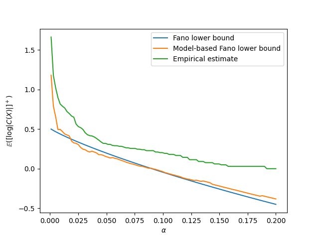
(a) CIFAR 10

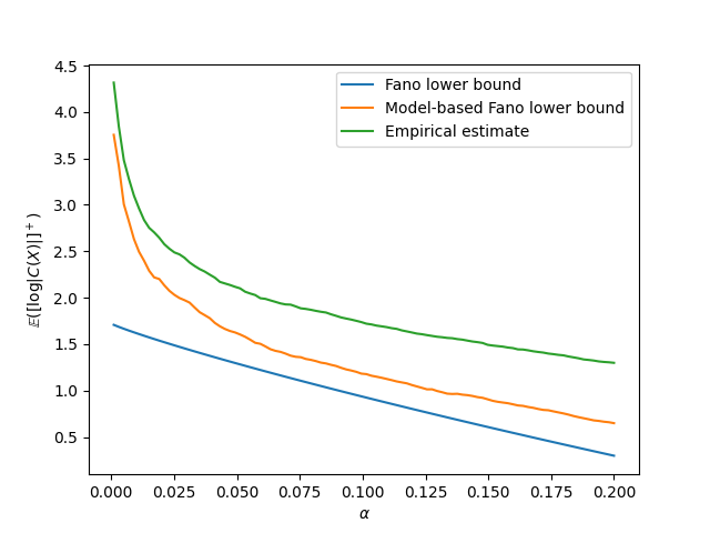
(b) CIFAR 100

Figure 2: Expected $[\log|C(X)|]^{+}$ as a function of $\alpha$.

Based on this, we evaluate our set size bounds on ResNet models trained with CE on CIFAR 10 and CIFAR 100. As the logits $\hat{Y}$ used for CP are not discrete, we perform K-means clustering on them and construct a vector quantized $\hat{Y}_{vq}$ by assigning to each logit vector its closest cluster centroid. We then use $\hat{Y}_{vq}$ to perform CP with thresholding and also use $\hat{Y}_{vq}$ to obtain a lower bound on $H(Y|\hat{Y}_{vq})$ via a maximum likelihood estimate for $H(Y,\hat{Y}_{vq})$. For this maximum likelihood estimate we also perform the Miller-Madow bias correction Paninski (2003).

For CIFAR 10 we cluster the logits into 32 clusters whereas for CIFAR 100 we use 256 clusters. The centroids are learned on a calibration set of 5k logits. For the model-based Fano bound, as it needs to compute terms that depend on the model probabilities and on whether the label was correctly covered by CP or not, we further split the calibration set into two equal-sized chunks; the first is used to find the quantile for thresholding and the second one is used to evaluate the terms of the bound. The obtained lower bounds on $[\log|C(X)|]^{+}$ for various $\alpha$’s can be seen at Figure 2. We also include an “empirical estimate” which is obtained by computing the quantile with the quantized calibration logits and then measuring the average $[\log|C(X)|]^{+}$ on the test set via thresholding on the quantized test logits. We can see that the model-based Fano provides relatively tight estimates for small values of alpha.

References

• Ahsan et al. (2022) Ahsan, M. M., Luna, S. A., and Siddique, Z. Machine-learning-based disease diagnosis: A comprehensive review. Healthcare, 10(3), 2022. ISSN 2227-9032. doi: 10.3390/healthcare10030541. URL https://www.mdpi.com/2227-9032/10/3/541.
• Ali & Silvey (1966) Ali, S. M. and Silvey, S. D. A General Class of Coefficients of Divergence of One Distribution from Another. Journal of the Royal Statistical Society. Series B (Methodological), 28(1):131–142, 1966. Publisher: [Royal Statistical Society, Wiley].
• Alnemer et al. (2016) Alnemer, L. M., Rajab, L., and Aljarah, I. Conformal prediction technique to predict breast cancer survivability. Int J Adv Sci Technol, 96:1–10, 2016.
• Angelopoulos et al. (2020) Angelopoulos, A., Bates, S., Malik, J., and Jordan, M. I. Uncertainty sets for image classifiers using conformal prediction. arXiv preprint arXiv:2009.14193, 2020.
• Angelopoulos & Bates (2021) Angelopoulos, A. N. and Bates, S. A gentle introduction to conformal prediction and distribution-free uncertainty quantification. arXiv preprint arXiv:2107.07511, 2021.
• Angelopoulos et al. (2021) Angelopoulos, A. N., Bates, S., Candès, E. J., Jordan, M. I., and Lei, L. Learn then test: Calibrating predictive algorithms to achieve risk control. arXiv preprint arXiv:2110.01052, 2021.
• Bastos (2024) Bastos, J. A. Conformal prediction of option prices. Expert Systems with Applications, 245:123087, 2024.
• Bates et al. (2021) Bates, S., Angelopoulos, A., Lei, L., Malik, J., and Jordan, M. Distribution-free, risk-controlling prediction sets. Journal of the ACM (JACM), 68(6):1–34, 2021. Publisher: ACM New York, NY.
• Bellotti (2021) Bellotti, A. Optimized conformal classification using gradient descent approximation. arXiv preprint arXiv:2105.11255, 2021.
• Blondel et al. (2020) Blondel, M., Teboul, O., Berthet, Q., and Djolonga, J. Fast differentiable sorting and ranking. In International Conference on Machine Learning, pp. 950–959. PMLR, 2020.
• Candès et al. (2021) Candès, E. J., Lei, L., and Ren, Z. Conformalized survival analysis. arXiv preprint arXiv:2103.09763, 2021.
• Cohen et al. (2017) Cohen, G., Afshar, S., Tapson, J., and Van Schaik, A. Emnist: Extending mnist to handwritten letters. In 2017 international joint conference on neural networks (IJCNN), pp.  2921–2926. IEEE, 2017.
• Collet (2019) Collet, J.-F. An Exact Expression for the Gap in the Data Processing Inequality for f -Divergences. IEEE Transactions on Information Theory, 65(7):4387–4391, July 2019. ISSN 1557-9654.
• Cover & Thomas (2006) Cover, T. M. and Thomas, J. A. Elements of information theory. Wiley-Interscience, Hoboken, N.J, 2nd ed edition, 2006.
• Csiszár (1967) Csiszár, I. On topological properties of f-divergence. Studia Sci. Math. Hungar., 2:330–339, 1967.
• Csiszár & Körner (2011) Csiszár, I. and Körner, J. Information theory: coding theorems for discrete memoryless systems. Cambridge University Press, Cambridge ; New York, 2nd ed edition, 2011.
• Cuturi et al. (2019) Cuturi, M., Teboul, O., and Vert, J.-P. Differentiable ranking and sorting using optimal transport. Advances in neural information processing systems, 32, 2019.
• Elias (1957) Elias, P. List Decoding for Noisy Channels. In IRE WESCON Convention Record, 1957, volume 2, pp. 94–104, 1957.
• Fano (1949) Fano, R. M. The transmission of information, volume 65. Massachusetts Institute of Technology, 1949.
• Gallager (1986) Gallager, R. G. Information theory and reliable communication. Wiley, New York, NY, 1986. ISBN 978-0-471-29048-3.
• Gupta et al. (2020) Gupta, C., Podkopaev, A., and Ramdas, A. Distribution-free binary classification: prediction sets, confidence intervals and calibration. Advances in Neural Information Processing Systems, 33:3711–3723, 2020.
• He et al. (2016) He, K., Zhang, X., Ren, S., and Sun, J. Deep residual learning for image recognition. In Proceedings of the IEEE conference on computer vision and pattern recognition, pp.  770–778, 2016.
• Humbert et al. (2023) Humbert, P., Le Bars, B., Bellet, A., and Arlot, S. One-shot federated conformal prediction. In International Conference on Machine Learning, pp. 14153–14177. PMLR, 2023.
• Krizhevsky et al. (2009) Krizhevsky, A. et al. Learning multiple layers of features from tiny images, 2009.
• Kuchibhotla (2020) Kuchibhotla, A. K. Exchangeability, conformal prediction, and rank tests. arXiv preprint arXiv:2005.06095, 2020.
• Kullback & Leibler (1951) Kullback, S. and Leibler, R. A. On information and sufficiency. The annals of mathematical statistics, 22(1):79–86, 1951.
• Kuutti et al. (2020) Kuutti, S., Bowden, R., Jin, Y., Barber, P., and Fallah, S. A survey of deep learning applications to autonomous vehicle control. IEEE Transactions on Intelligent Transportation Systems, 22(2):712–733, 2020.
• LeCun et al. (1998) LeCun, Y., Bottou, L., Bengio, Y., and Haffner, P. Gradient-based learning applied to document recognition. Proceedings of the IEEE, 86(11):2278–2324, 1998.
• Lei et al. (2015) Lei, J., Rinaldo, A., and Wasserman, L. A conformal prediction approach to explore functional data. Annals of Mathematics and Artificial Intelligence, 74:29–43, 2015.
• Lei et al. (2018) Lei, J., G’Sell, M., Rinaldo, A., Tibshirani, R. J., and Wasserman, L. Distribution-free predictive inference for regression. Journal of the American Statistical Association, 113(523):1094–1111, 2018.
• Lei & Candès (2021) Lei, L. and Candès, E. J. Conformal inference of counterfactuals and individual treatment effects. Journal of the Royal Statistical Society: Series B (Statistical Methodology), 2021. Publisher: Wiley Online Library.
• Li et al. (2022) Li, Q., Diao, Y., Chen, Q., and He, B. Federated learning on non-iid data silos: An experimental study. In 2022 IEEE 38th International Conference on Data Engineering (ICDE), pp.  965–978. IEEE, 2022.
• Liese & Vajda (2006) Liese, F. and Vajda, I. On Divergences and Informations in Statistics and Information Theory. IEEE Transactions on Information Theory, 52(10):4394–4412, October 2006.
• Liu et al. (2017) Liu, J., Cuff, P., and Verdú, S. $e_{\gamma}$-Resolvability. IEEE Transactions on Information Theory, 63(5):2629–2658, May 2017. Conference Name: IEEE Transactions on Information Theory.
• Louizos et al. (2024) Louizos, C., Reisser, M., and Korzhenkov, D. A mutual information perspective on federated contrastive learning. In The Twelfth International Conference on Learning Representations, 2024. URL https://openreview.net/forum?id=JrmPG9ufKg.
• Lu & Kalpathy-Cramer (2021) Lu, C. and Kalpathy-Cramer, J. Distribution-free federated learning with conformal predictions. arXiv preprint arXiv:2110.07661, 2021.
• Lu et al. (2022a) Lu, C., Angelopoulos, A. N., and Pomerantz, S. Improving trustworthiness of ai disease severity rating in medical imaging with ordinal conformal prediction sets. In International Conference on Medical Image Computing and Computer-Assisted Intervention, pp.  545–554. Springer, 2022a.
• Lu et al. (2022b) Lu, C., Lemay, A., Chang, K., Höbel, K., and Kalpathy-Cramer, J. Fair conformal predictors for applications in medical imaging. In Proceedings of the AAAI Conference on Artificial Intelligence, volume 36, pp.  12008–12016, 2022b.
• maintainers & contributors (2016) maintainers, T. and contributors. Torchvision: Pytorch’s computer vision library. https://github.com/pytorch/vision, 2016.
• Maurer & Pontil (2009) Maurer, A. and Pontil, M. Empirical bernstein bounds and sample variance penalization. arXiv preprint arXiv:0907.3740, 2009.
• McMahan et al. (2017) McMahan, B., Moore, E., Ramage, D., Hampson, S., and y Arcas, B. A. Communication-efficient learning of deep networks from decentralized data. In Artificial intelligence and statistics, pp.  1273–1282. PMLR, 2017.
• Merhav (2014) Merhav, N. List Decoding—Random Coding Exponents and Expurgated Exponents. IEEE Transactions on Information Theory, 60(11):6749–6759, November 2014. ISSN 1557-9654. Conference Name: IEEE Transactions on Information Theory.
• Morimoto (1963) Morimoto, T. Markov Processes and the H-Theorem. Journal of the Physical Society of Japan, 18(3):328–331, March 1963. Publisher: The Physical Society of Japan.
• Moritz et al. (2018) Moritz, P., Nishihara, R., Wang, S., Tumanov, A., Liaw, R., Liang, E., Elibol, M., Yang, Z., Paul, W., Jordan, M. I., et al. Ray: A distributed framework for emerging $\{$AI$\}$ applications. In 13th USENIX symposium on operating systems design and implementation (OSDI 18), pp.  561–577, 2018.
• Paninski (2003) Paninski, L. Estimation of entropy and mutual information. Neural computation, 15(6):1191–1253, 2003.
• Papadopoulos et al. (2002) Papadopoulos, H., Proedrou, K., Vovk, V., and Gammerman, A. Inductive confidence machines for regression. In Machine Learning: ECML 2002: 13th European Conference on Machine Learning Helsinki, Finland, August 19–23, 2002 Proceedings 13, pp. 345–356. Springer, 2002.
• Papadopoulos et al. (2009) Papadopoulos, H., Gammerman, A., and Vovk, V. Reliable diagnosis of acute abdominal pain with conformal prediction. Engineering Intelligent Systems, 17(2):127, 2009.
• Paszke et al. (2017) Paszke, A., Gross, S., Chintala, S., Chanan, G., Yang, E., DeVito, Z., Lin, Z., Desmaison, A., Antiga, L., and Lerer, A. Automatic differentiation in pytorch. In NIPS-W, 2017.
• Petersen et al. (2022) Petersen, F., Borgelt, C., Kuehne, H., and Deussen, O. Monotonic differentiable sorting networks. In International Conference on Learning Representations (ICLR), 2022.
• Polyanskiy & Wu (2014) Polyanskiy, Y. and Wu, Y. Lecture notes on information theory. Lecture Notes for ECE563 (UIUC) and, 6(2012-2016):7, 2014.
• Polyanskiy et al. (2010) Polyanskiy, Y., Poor, H. V., and Verdu, S. Channel Coding Rate in the Finite Blocklength Regime. IEEE Transactions on Information Theory, 56(5):2307–2359, May 2010.
• Raginsky & Sason (2013) Raginsky, M. and Sason, I. Concentration of measure inequalities in information theory, communications, and coding. Number vol. 10, no. 1-2 in Foundations and Trends in Communications and Information Theory. Now Publ, Boston, Mass., 2013. ISBN 978-1-60198-724-2.
• Romano et al. (2019) Romano, Y., Patterson, E., and Candes, E. Conformalized quantile regression. Advances in neural information processing systems, 32, 2019.
• Romano et al. (2020) Romano, Y., Sesia, M., and Candes, E. Classification with valid and adaptive coverage. Advances in Neural Information Processing Systems, 33:3581–3591, 2020.
• Sadinle et al. (2019) Sadinle, M., Lei, J., and Wasserman, L. Least ambiguous set-valued classifiers with bounded error levels. Journal of the American Statistical Association, 114(525):223–234, 2019.
• Sason (2019) Sason, I. On data-processing and majorization inequalities for f-divergences with applications. Entropy, 21(10):1022, 2019. Publisher: MDPI.
• Sason & Verdú (2016) Sason, I. and Verdú, S. f-Divergence Inequalities. IEEE Transactions on Information Theory, 62(11):5973–6006, November 2016.
• Sason & Verdú (2017) Sason, I. and Verdú, S. Arimoto–Rényi conditional entropy and Bayesian M -ary hypothesis testing. IEEE Transactions on Information theory, 64(1):4–25, 2017. Publisher: IEEE.
• Shafer & Vovk (2008) Shafer, G. and Vovk, V. A tutorial on conformal prediction. Journal of Machine Learning Research, 9(3), 2008.
• Stutz et al. (2022) Stutz, D., Dvijotham, K. D., Cemgil, A. T., and Doucet, A. Learning optimal conformal classifiers. In International Conference on Learning Representations, 2022.
• Tibshirani et al. (2019) Tibshirani, R. J., Foygel Barber, R., Candes, E., and Ramdas, A. Conformal prediction under covariate shift. Advances in neural information processing systems, 32, 2019.
• Vovk et al. (2005) Vovk, V., Gammerman, A., and Shafer, G. Algorithmic learning in a random world, volume 29. Springer, 2005.
• Vovk et al. (2016) Vovk, V., Fedorova, V., Nouretdinov, I., and Gammerman, A. Criteria of efficiency for conformal prediction. In Conformal and Probabilistic Prediction with Applications: 5th International Symposium, COPA 2016, Madrid, Spain, April 20-22, 2016, Proceedings 5, pp.  23–39. Springer, 2016.
• Wang et al. (2021) Wang, J., Charles, Z., Xu, Z., Joshi, G., McMahan, H. B., Al-Shedivat, M., Andrew, G., Avestimehr, S., Daly, K., Data, D., et al. A field guide to federated optimization. arXiv preprint arXiv:2107.06917, 2021.
• Wisniewski et al. (2020) Wisniewski, W., Lindsay, D., and Lindsay, S. Application of conformal prediction interval estimations to market makers’ net positions. In Conformal and Probabilistic Prediction and Applications, pp.  285–301. PMLR, 2020.
• Wozencraft (1958) Wozencraft, J. M. List decoding. PhD thesis, Research Laboratory of Electronics, MIT, Cambridge, MA, USA, January 1958. Publisher: Research Laboratory of Electronics, MIT.
• Xiao et al. (2017) Xiao, H., Rasul, K., and Vollgraf, R. Fashion-mnist: a novel image dataset for benchmarking machine learning algorithms. arXiv preprint arXiv:1708.07747, 2017.