Multi-rate Runge-Kutta methods:
stability analysis and applications

Abstract

We present an approach for the efficient implementation of self-adjusting multi-rate Runge-Kutta methods and we extend the previously available stability analyses of these methods to the case of an arbitrary number of sub-steps for the active components. We propose a physically motivated model problem that can be used to assess the stability of different multi-rate versions of standard Runge-Kutta methods and the impact of different interpolation methods for the latent variables. Finally, we present the results of several numerical experiments, performed with implementations of the proposed methods in the framework of the OpenModelica open-source modelling and simulation software, which demonstrate the efficiency gains deriving from the use of the proposed multi-rate approach for physical modelling problems with multiple time scales.

⁽¹⁾ Faculty of Engineering and Mathematics
University of Applied Sciences and Arts, Bielefeld, Germany
bernhard.bachmann@hsbi.de

⁽²⁾ Dipartimento di Matematica
Politecnico di Milano
luca.bonaventura@polimi.it

⁽³⁾ Dipartimento di Elettronica, Informazione e Bioingegneria
Politecnico di Milano
casella@elet.polimi.it

⁽⁴⁾ Departamento de Ecuaciones Diferenciales y Análisis Numérico & IMUS,
Universidad de Sevilla
soledad@us.es

⁽⁵⁾ Departamento de Ecuaciones Diferenciales y Análisis Numérico,
Universidad de Sevilla
macarena@us.es

Keywords: Multi-rate methods, multi-scale problems, stiff ODE problems, Runge-Kutta methods, ESDIRK methods

AMS Subject Classification: 65L04, 65L05, 65L07, 65M12, 65M20

1 Introduction

We consider in this work numerical methods for systems of Ordinary Differential Equations (ODEs) that can be partitioned into components $y_{s},y_{f}$ with slow and fast dynamics, respectively, as

$${y}^{\prime}=\left[\begin{array}[]{ll}{y}^{\prime}_{{s}}\\ {y}^{\prime}_{f}\end{array}\right]=\left[\begin{array}[]{ll}{f}_{{s}}({y}_{s},{y}_{{f}},t)\\ {f}_{f}({y}_{s},{y}_{{f}},t)\end{array}\right]=f(y,t)$$ (1.1)

for $t\in[0,T].$ For such systems, several methods have been proposed in which different time steps are employed for the slow and fast components. These are generically known as multi-rate methods, as opposed to standard single-rate methods for ODEs. Variables $y_{s},y_{f}$ are also known in the literature as latent and active variables, respectively. Approaches based on this concept have been proposed over the last 60 years, see e.g. [1, 7, 19]. More recently, a number of methods have been proposed that do not require a priori partitioning as in (1.1), but rather allow to identify fast and slow variables at runtime by their compliance, or lack of compliance, with a given error indicator, so that the system has form (1.1) with a right-hand side partition that can be different for each time discretization interval. A review of these methods is presented in [5], where a variant of this more general, self-adjusting multi-rate approach was introduced. The proposal in [5] was tailored on the specific implicit TR-BDF2 method [4, 9], along with a general stability analysis for one-step multi-rate methods.

The aim of the present work is a further generalization of the results in [5]. Firstly, we propose a simplified and improved version of the self-adjusting multi-rate procedure introduced in [5], which allows to obtain a more effective multi-rate implementation of a generic Runge-Kutta (RK) method. The novel approach combines a self-adjusting multi-rate technique with standard time step adaptation methods, by marking as fast variables only a small percentage of the variables associated with the largest values of an error estimator. Whenever the global time step is sufficient to guarantee a given error tolerance for the slow variables, but not for the fast ones, the multi-rate procedure is employed to achieve uniform accuracy at reduced computational cost. This approach is similar to that used successfully in (spatially) adaptive finite element techniques, see e.g. [2, 3, 16, 15], where a fixed percentage of the simulation Degrees of Freedom (DOF) can be marked for refinement if error indicator values exceed a given tolerance.

We then extend the stability analysis of [5] to the case of an arbitrary number of sub-steps for the active components. This analysis covers the case of Explicit RK methods (ERK), Diagonally Implicit RK methods (DIRK) and Singly Diagonally Implicit Runge Kutta methods with Explicit first stage (ESDIRK). In order to apply this methodology to a case that is relevant for applications, we propose a physically motivated model problem that can be used to assess the stability of different multi-rate versions of standard RK methods and the impact of different interpolation methods for the latent variables. We perform the stability analysis of some sample methods, highlighting the fact that, in regimes of weak coupling between fast and slow variables and in presence of some dissipation, multi-rate approaches generally maintain the stability properties of the corresponding single-rate methods.

Finally, we apply the proposed methods to a number of numerical benchmark problems. For this purpose, we use an implementation of the proposed approach in the framework of the OpenModelica software [6]. Due to their computational advantages, we will focus in particular on the application of multi-rate versions of higher order ESDIRK methods. A very comprehensive review of these methods was presented in [11, 12], where the properties and potential advantages of this class of methods are discussed in detail. The results demonstrate the efficiency gains deriving from the use of the proposed multi-rate approach for problems with multiple time scales.

The outline of the paper is the following. In Section 2, the self-adjusting multi-rate approach is presented. In Section 3, a linear stability analysis of the proposed methods is performed, which considers an arbitrary number of sub-steps for the active variables. In Section 4, a specific model problem is considered, to which the previously introduced analysis template is applied. The resulting analysis highlights the impact on multi-rate stability of the different choices for the interpolation operator of the latent variables and of the number of sub-steps for the active variables. In Section 5, numerical results are shown, which demonstrate the good performance of the proposed methods even against optimal implementations of single-rate solvers. In Section 6, we summarize our results and discuss possible future developments.

2 Effective implementation of multi-rate methods

Multi-rate methods have been defined in a number of previous papers. Here, we follow the general outline of [5], but we introduce several simplifications and extensions which allow to achieve a more efficient implementation. We consider again the generic nonlinear system ${y}^{\prime}=f(y,t),$ where $y:[0,T]\rightarrow\mathbb{R}^{N}$ is the solution of the continuous first order ODE problem and $f:\mathbb{R}^{N}\times[0,T]\rightarrow\mathbb{R}^{N}$ the ODE right-hand side, which is assumed to satisfy the usual regularity requirements to guarantee local existence and smoothness of the solutions. Let then $t_{n},n\in\mathbb{N}$ denote a set of discrete time levels such that $t_{0}=0,$ $t_{n+1}=t_{n}+h_{n}$ and $h_{n}$ denotes a generic time step. At each time level $n,$ two approximations $u_{n+1}$ and $\hat{u}_{n+1}$ of the solution $y(t_{n+1})$ are computed, with convergence orders $p$ and $\hat{p},$ respectively. We set $q=\min(p,\hat{p}).$ In the case of RK methods, approximation $\hat{u}_{n+1}$ is usually obtained from an embedded method, see e.g. [8], to which we refer for all the general concepts on ODE methods used in the following. An error estimator for the less accurate approximation is then given by $\|u_{n+1}-\hat{u}_{n+1}\|$.

In standard single-rate implementations of RK methods, in order to comply with assigned error tolerances $\tau^{r},$ $\tau^{a}$ for relative and absolute errors, respectively, one introduces for each time step $i=1,\dots,N$ the quotient

$$\eta^{n+1}_{i}=\frac{|u^{n+1}_{i}-\hat{u}^{n+1}_{i}|}{\tau^{r}|u^{n+1}_{i}|+\tau^{a}}$$ (2.1)

and requires that the inequality

$$\eta=\max_{i=1,\dots,N}\eta_{i}^{n+1}\leq 1$$

holds. An optimal choice of the new time step value for an adaptive single-rate implementation is then given by

$$h_{new}=h_{n}\eta^{-\frac{1}{q+1}}.$$

If $\eta\leq 1$ is satisfied, the solution is advanced with $u_{n+1}$ and the new step size is chosen as $h_{n+1}=h_{new}$. Notice that, in practice, some user defined safety parameter $\beta\in(0,1)$ will be introduced so that the condition to accept the new time step will be $\eta\leq\beta.$ Otherwise, the step is rejected and the computation is repeated with $h_{n}=h_{new}$. In practice, the optimal step size is calculated using some safety factors, so that

$$h_{new}=h_{n}\min\{\alpha_{max},\max\{\alpha_{min},\alpha\eta^{-\frac{1}{q+1}}\}\}.$$ (2.2)

Reasonable default values of the safety factors can be selected as $\alpha_{max}=1.2$, $\alpha_{min}=0.5$, and $\alpha=0.9$. It is important to remark that, in the application of these definitions in a multi-rate framework, the value of $\alpha_{min}$ has an impact on the maximum number of sub-steps chosen for the active components, so that it may have to be adjusted depending on the time scales involved in the specific problem to be solved.

In order to define the multi-rate extension of a given RK method, we denote by

$${u}_{n+1}={\cal S}({u}_{n},h_{n}),\ \ {\cal S}:\mathbb{R}^{N}\times\mathbb{R}^{+}\rightarrow\mathbb{R}^{N}$$

the global step of the basic single-rate method. We will denote as ${\cal V}^{f}_{n}\subset\mathbb{R}^{N}$ the linear subspace of fast variables at time level $n.$ It is implicitly assumed that $d_{n}={\rm dim}({\cal V}^{f}_{n})<<N.$ We also denote as $P^{f}_{n}:\mathbb{R}^{N}\rightarrow\mathbb{R}^{d_{n}}$ the projector on the linear subspace of fast variables, while ${P}^{s}_{n}:\mathbb{R}^{N}\rightarrow\mathbb{R}^{N-d_{n}}$ denotes the projection on the linear subspace of slow variables ${\cal V}_{n}^{s}.$ For brevity, we will also denote ${u}^{s}_{n}={P}^{s}_{n}u_{n}$ and ${u}^{f}_{n}={P}^{f}_{n}u_{n}.$ The operator

$${u}^{f}_{n+1}={\cal S}^{f}({u}^{f}_{n},w,h_{n}):\mathbb{R}^{d_{n}}\times\mathbb{R}^{N-{d_{n}}}\rightarrow\mathbb{R}^{d_{n}}$$

will then denote the application of the basic method ${\cal S}$ to the subsystem of $y^{\prime}=f(y,t)$ obtained by projecting ${u}_{n}$ onto ${\cal V}_{n}^{f}$ and assuming that the remaining components of ${u}_{n}$ belonging to ${\cal V}_{n}^{s}$ are given by the given vector $w.$ Furthermore, setting $\zeta=t_{n}+\tau h_{n}$ for each $\tau\in[0,1],$ we will denote as $Q(\tau)$ a generic operator that interpolates known values of slow variables at time level $\zeta.$ This operator is used to provide intermediate values of the slow variables for the application of ${\cal S}^{f}$ and can be given, for example, by the dense output approximation associated to a given ODE method, see e.g. [8] for relevant examples. Given these definitions, the general multi-rate approach we will implement can be defined as in the following pseudo-code.

Multirate algorithm:

1. Compute a tentative global step $u_{n+1}={\cal S}({u}_{n},h_{n})$ and the additional approximation $\hat{u}_{n+1}$.

2. For each component $u^{n+1}_{i},i=1,\dots,N,$ compute the error estimation $\eta^{n+1}_{i}$ as described in expression (2.1).

3. Let ${\tilde{\eta}}^{n+1}_{i}$ denote the components of a vector obtained sorting $\eta_{n+1}$ in descending order and $s=s(i),i=1,\dots,N,$ the map that assigns to each component of $\eta_{n+1}$ the index of its location in ${\tilde{\eta}}_{n+1}.$ Define $m\in\{1,\dots,N\}$ as the only integer such that $m/N\leq\phi<(m+1)/N,$ where $\phi\in(0,1)$ is a user defined parameter determining the maximum fraction of fast variables that will be allowed in the simulation. Define also the index subset

   $${\cal S}_{n}=\{i\in\{1,\dots,N\}:s(i)>m\}.$$

4. If

   $$\eta_{s}=\max_{i\in{\cal S}_{n}}\eta_{i}^{n+1}>\beta,$$

   reject the global time step and recompute it using the time step given by expression (2.2) with respect to $\eta_{s}$.

5. If

   $$\eta_{f}=\max_{i\in{\cal S}_{n}^{\;c}}\eta_{i}^{n+1}\leq\beta,$$

   accept the global time step and compute the next using the time step given by expression (2.2) with respect to $\eta_{s}$.

6. If $\eta_{s}\leq\beta$ and $\eta_{f}>\beta,$ go multirate:

   • Define ${\cal V}^{f}_{n}$ as the subspace of $\mathbb{R}^{N}$ whose coordinates have indices $i$ such that $\eta_{i}^{n+1}>\beta$ and ${\cal V}_{n}^{s}={{\cal V}^{f}_{n}}^{\,c}$ and ${\cal S}_{n}^{f}$ the corresponding index subset. Notice that ${\cal S}_{n}^{f}\subset{\cal S}_{n}^{\;c}.$

   • Partition the state space as $\mathbb{R}^{N}={\cal V}^{f}_{n}\oplus{\cal V}_{n}^{s},$ and set ${u}^{s}_{n+1}=P^{s}_{n}{u}_{n+1};$

   • Set ${u}^{f}_{n,0}={u}^{f}_{n}.$ Compute ${u}^{f}_{n,l+1}={\cal S}^{f}({u}^{f}_{n,l},{u}^{s}_{n,l},h_{n}^{f})$ with local time steps determined using time step control based on expression (2.2) with respect to

     $$\hat{\eta}=\max_{i\in{\cal S}_{n}^{f}}\eta_{i}^{n,l+1}.$$

   • Proceed until the time of the global time step has been reached. Apply the same logic for step rejection and acceptance (see 4) and 5)) with respect to $\hat{\eta}.$ Compute necessary values of the slow variables at intermediate time levels using the interpolation operator $Q(.)$. Let $M_{n}$ denote the number of local steps taken.

   • Set ${u}^{f}_{n+1}={u}^{f}_{n,M_{n}}$ and determine a new global time step based on expression (2.2) with respect to $\eta_{s}$, then go to 1).

As remarked previously, the value of $\alpha_{min}$ plays a role in determining the maximum number of sub-steps performed for the active variables. Therefore, it may need to be adjusted depending on specific accuracy or stability features of the method or problem under consideration. Furthermore, as discussed in Section 1, the set of active variables is chosen here in a way that has already proven to be successful in adaptive finite element techniques, see e.g. [2, 3, 16, 15]. This enables us to reduce or avoid conflicts between the global time step adaptation and the multi-rate strategy, which is instead employed to achieve the same level of accuracy as the corresponding single-rate implementation at a reduced computational cost.

Last, but not least, an important remark is due for the case of strongly non-linear ODEs and implicit Runge-Kutta multi-rate integration methods. The equations of implicit Runge-Kutta methods are solved via iterative Newton-Raphson algorithms, with an initial guess computed by extrapolation of the solution found at previous time steps. In case the RHS $f(y,t)$ of the ODEs is strongly non-linear, this may cause convergence problems or even failure if the time step is too large, because the initial guess will be too far from the solution.

This issue is much more critical for multi-rate integration, since the global time step is chosen without considering the errors of the variables belonging to the fast partition, so it is in general much larger than in the case of single-rate methods. It therefore essential to limit the maximum number of Newton iterations to a relatively low value such as 20, after which a shorter time step should be attempted; otherwise, a large amount of time and computational effort can end up being wasted in the futile attempt to achieve convergence from an initial guess which is too far from the solution. It is also advisable to choose conservative values of $\alpha_{max}$, such as $\alpha_{max}=1.2$, to avoid getting again into convergence issues at the next global time step.

3 Stability analysis

Several stability analyses of multi-rate methods have been presented in the literature, see e.g. [10, 13, 20]. These works however focus on the complete analysis of systems with just two degrees of freedom, which strongly limits the relevance of these analyses for more realistic applications. In [5], an approach was introduced that allows to build, at least numerically, the stability function of a multi-rate method for an arbitrary linear ODE system. Here, we revisit the stability analysis presented in [5] and we generalize it to the case of a multi-rate procedure with an arbitrary number of sub-steps based on a generic ERK, DIRK or ESDIRK method.

We consider a generic linear homogeneous, constant coefficient ODE system $y^{\prime}=Ly$ with $y\in{\mathbb{R}}^{N},$ $L\in{\cal M}_{N,N}(\mathbb{R})$ and $\sigma(L)\subset\mathbb{R}^{-}\cup\{0\}.$ This assumption will allow to consider also systems with purely oscillatory behaviour, for which the application of multi-rate techniques is of great practical interest. We assume that the state space is partitioned a priori as ${\mathbb{R}}^{N}={\cal V}_{s}\oplus{\cal V}_{f},$ where ${\cal V}_{s}$ denotes the subspace of the slow or latent variables and ${\cal V}_{f}$ denotes the subspace of the fast or active variables. We also set $d={\rm dim}({\cal V}_{f}).$ Introducing the identity matrix ${\mathbb{I}}_{m}\in{\cal M}_{m,m}(\mathbb{R})$ and the zero matrix ${\mathbb{O}}_{m,n}\in{\cal M}_{m,n}(\mathbb{R}),$ one can represent the projections onto ${\cal V}_{s},{\cal V}_{f}$ by the matrices

$$P_{s}=\left[\begin{array}[]{lcl}{\mathbb{I}}_{N-d}&{\mathbb{O}}_{N-d,d}\end{array}\right]\ \ \ \ P_{f}=\left[\begin{array}[]{lcl}{\mathbb{O}}_{d,N-d}&{\mathbb{I}}_{d}\end{array}\right]$$ (3.1)

and the corresponding embedding operators of ${\cal V}_{s},{\cal V}_{f}$ into ${\mathbb{R}}^{N}$ by $P_{s}^{T},P_{f}^{T},$ respectively, as often done in the literature on domain decomposition methods, see e.g. [18]. As a consequence, $P_{s}^{T}P_{s}$ is the operator that sets to zero all the components of a vector in ${\mathbb{R}}^{N}$ corresponding to the fast variables; $P_{f}^{T}P_{f}$ acts analogously on the slow variables and $P_{s}^{T}P_{s}+P_{f}^{T}P_{f}={\mathbb{I}}_{N}.$ This entails that the model system $y^{\prime}=Ly$ can be written in terms of the partitioned matrix

$$L=\left[\begin{array}[]{lccl}P_{s}LP_{s}^{T}&P_{s}LP^{T}_{f}\\ P_{f}LP_{s}^{T}&P_{f}LP^{T}_{f}\end{array}\right]=\left[\begin{array}[]{lccl}L_{ss}&L_{sf}\\ L_{fs}&L_{ff}\end{array}\right],$$ (3.2)

or, equivalently, introducing the notation $y_{f}=P_{f}y,$ $y_{s}=P_{s}y,$ as

$$y_{s}^{\prime} = P_{s}LP_{s}^{T}y_{s}+P_{s}LP_{f}^{T}y_{f}$$

$$y_{f}^{\prime} = P_{f}LP_{s}^{T}y_{s}+P_{f}LP_{f}^{T}y_{f}.$$ (3.3)

We assume that at a given time level $t_{n}$ a time step $h=h_{s}$ is employed for the slow variables and $h_{f}=h_{s}/M$ for the $l=0,\dots,M$ substeps of the fast variables, corresponding to the time levels $t_{n+l}=t_{n}+lh^{f}.$ If the multi-rate method is based on a generic one step time discretization method whose amplification function can be written as $R(z)={N(z)}/{D(z)},$ where $N,D$ are polynomials in $z,$ the value of the slow variables at the new time steps is given by $u_{n+1}^{s}=P_{s}R(h_{s}L)u_{n}.$ As discussed in Section 2, values $u_{n+\tau}$ at intermediate time levels $\zeta=t_{n}+\tau h_{s}\in[t_{n},t_{n+1}],$ where $\tau\in[0,1]$ denotes the fraction of the global time step at which the interpolated value is required, can be computed from the values of $u_{n},u_{n+1}$ by appropriate interpolation techniques, represented formally by a family of operators parameterized by $\tau:$

$$Q(\tau):\mathbb{R}^{N}\rightarrow\mathbb{R}^{N}.$$

The simplest example of such operator is given by linear interpolation. Since in this case

$$u_{n+\tau}=(1-\tau)u_{n}+\tau u_{n+1}=(1-\tau)u_{n}+\tau R(h_{s}L)u_{n},$$

interpolation can be represented in this case by the application of the operator

$$Q(\tau)=(1-\tau)\mathbb{I}_{N}+\tau R(h_{s}L)$$ (3.4)

to $u_{n}.$ The slow variables at intermediate substeps are then given by $u_{n+\tau}^{s}=P_{s}Q(\tau)u_{n}.$ Another simple option is cubic Hermite interpolation, which is easy to implement and convenient for methods up to fourth order. In this case, also approximations of $y^{\prime}(t_{n+1}),$ $y^{\prime}(t_{n})$ are needed, which are provided by $Lu_{n+1}$ and $Lu_{n}.$ The interpolation operator reads in this case:

$$Q(\tau) = (1+2\tau)(1-\tau)^{2}\mathbb{I}_{N}+(3-2\tau)\tau^{2}R(h_{s}L)$$ (3.5)

$$+ h_{s}\tau(1-\tau)^{2}L+h_{s}(\tau-1)\tau^{2}LR(h_{s}L).$$

It should be remarked, however, that the analysis presented in [13] shows how Hermite interpolation may introduce instabilities in multi-rate procedures. More accurate interpolation procedures are provided by dense output versions of the approximation methods considered, see e.g. [8] for a general discussion and [11] for the details of some dense output DIRK and ESDIRK methods. The precise definition of the $Q(\tau)$ operators associated to dense output interpolators will be described in the following.

The goal of the stability analysis will be to represent the discrete time evolution as $u_{n+1}=R_{mr}u_{n},$ where $R_{mr}$ will depend on $h_{s},M,$ $L,$ and on the specific properties of the time discretization and interpolation method employed. Since $u_{n+1}^{s}=P_{s}R(h_{s}L)u_{n}$ and $P_{s}^{T}P_{s}+P_{f}^{T}P_{f}={\mathbb{I}}_{N},$ one has

$$u^{s}_{n+1}=P_{s}R(h_{s}L)P_{s}^{T}u^{s}_{n}+P_{s}R(h_{s}L)P_{f}^{T}u^{f}_{n},$$ (3.6)

so that the multi-rate amplification matrix will have the form

$$R_{mr}=\left[\begin{array}[]{lccl}P_{s}R(h_{s}L)P_{s}^{T}&P_{s}R(h_{s}L)P_{f}^{T}\\ R_{fs}&R_{ff}\end{array}\right],$$ (3.7)

where the operators $R_{fs}$ and $R_{ff}$ depend on the specific properties of the basic single-rate method on which the multi-rate method is based and of the interpolation operator.

We will outline the stability analysis for generic ERK, DIRK and ESDIRK methods, identified as customary by their Butcher tableaux. These consist of $A\in{\cal M}_{s,s}(\mathbb{R})$ and $b,c\in\mathbb{R}^{s},$ where $s$ is the number of stages and the usual simplifying hypotheses are implicitly assumed, see e.g. [8]. The single-rate method applied to problem $y^{\prime}=f(y,t)$ can therefore be written, following [12], as

$$U^{(i)} = u_{n}+h\sum_{j=1}^{s}a_{i,j}f(U^{(j)},t_{n}+c_{j}h)\ \ \ \ \ i=1,\dots,s$$

$$u_{n+1} = u_{n}+h\sum_{i=1}^{s}b_{i}f(U^{(i)},t_{n}+c_{i}h).$$ (3.8)

In the linear case $y^{\prime}=Ly$ this yields

$$U^{(i)} = u_{n}+h\sum_{j=1}^{s}a_{i,j}LU^{(j)}\ \ \ \ \ i=1,\dots,s$$

$$u_{n+1} = u_{n}+h\sum_{i=1}^{s}b_{i}LU^{(i)}.$$ (3.9)

A dense output approximation of $y$ at time level $\zeta=t_{n}+\tau h_{s},$ see again [8, 11], can be written as

$$u_{n+\tau}=u_{n}+h\sum_{i=1}^{s}b^{*}_{i}(\tau)LU^{(i)},\ \ i=1,\dots,s$$

with $b^{*}_{i}(\tau)=\sum_{j=1}^{p^{*}}b^{*}_{i,j}\tau^{j}$ for appropriate method specific values of $p^{*}$ and $b^{*}_{i,j}.$ For ERK methods

$${R}^{(1)}=\mathbb{I}\ \ \ \ \ {R}^{(k)}=\mathbb{I}+h\sum_{j=1}^{k-1}a_{k,j}L{R}^{(j)},$$ (3.10)

so that $U^{(i)}={R}^{(i)}u_{n}.$ As a consequence, the operator representation of the dense output interpolator can be written as

$$Q(\tau)=\mathbb{I}+h\sum_{i=1}^{s}b^{*}_{i}(\tau)L{R}^{(i)}.$$ (3.11)

For DIRK methods one defines instead

$${R}^{(1)} = \left(\mathbb{I}-ha_{k,k}L\right)^{-1}$$

$${R}^{(k)} = \left(\mathbb{I}-ha_{k,k}L\right)^{-1}\left[\mathbb{I}+h\sum_{j=1}^{k-1}a_{k,j}L{R}^{(j)}\right],\ \ k\geq 2,$$ (3.12)

so that again the dense output interpolator can be represented by formula (3.11), where this definition of the ${R}^{(k)}$ operator is employed. By the same reasoning that allows to derive (3.11), one also has that

$$R(hL)=\mathbb{I}+h\sum_{i=1}^{s}b_{i}L{R}^{(i)}.$$ (3.13)

Notice that formulae (3) and (3.13) are actually valid also for the ERK case, by simply assuming $a_{i,i}=0,i=1,\dots,s,$ and in the case of ESDIRK methods, by assuming $a_{1,1}=0.$ This will allow to simplify the following stability analysis, which will be carried out explicitly for DIRK methods only, but whose results are also valid for ERK and ESDIRK methods again with appropriate assumptions on the Butcher tableaux.

For the corresponding multi-rate methods, denoting again by $R$ the amplification function of the single-rate method, for the linear problem $y^{\prime}=Ly$ the slow variables can be computed as discussed previously by $u^{s}_{n+1}=P_{s}R(h_{s}L)P_{s}^{T}u^{s}_{n}+P_{s}R(h_{s}L)P_{f}^{T}u^{f}_{n}.$ For the fast variables, assuming that

$$U^{(i,l)}_{s}\approx P_{s}Q((l+c_{i})/M)u_{n}$$

for $i=1,\dots,s,$ and $l=0,\dots,M-1,$ and setting $Q^{(i,l)}=Q((l+c_{i})/M)$ for brevity, one has

$$U^{(i,l)}_{f}=u^{f}_{n,l} + h_{f}\sum_{j=1}^{s}a_{i,j}L_{ff}U_{f}^{(j,l)}+h_{f}\sum_{j=1}^{s}a_{i,j}L_{fs}P_{s}Q^{(j,l)}u_{n}$$

$$u_{n,l+1}^{f}=u^{f}_{n,l} + h_{f}\sum_{i=1}^{s}b_{i}L_{ff}U_{f}^{(i,l)}+h_{f}\sum_{i=1}^{s}b_{i}L_{fs}P_{s}Q^{(i,l)}u_{n}.$$ (3.14)

In order to derive an explicit expression for the amplification matrix of the multi-rate method, we will now consider the specific case of DIRK methods, which as explained before allows to derive formulae that are also valid for ERK and ESDIRK methods. From the basic definitions it follows that

$$U^{(1,l)}_{f} = u^{f}_{n,l}+h_{f}a_{1,1}L_{ff}U_{f}^{(1,l)}+h_{f}a_{1,1}L_{fs}P_{s}Q^{(1,l)}u_{n}$$

$$U^{(2,l)}_{f} = u^{f}_{n,l}+h_{f}a_{2,1}L_{ff}U_{f}^{(1,l)}+h_{f}a_{2,1}L_{fs}P_{s}Q^{(1,l)}u_{n}$$

$$+ h_{f}a_{2,2}L_{ff}U_{f}^{(2,l)}+h_{f}a_{2,2}L_{fs}P_{s}Q^{(2,l)}u_{n}$$

$$\dots$$

$$U^{(s,l)}_{f} = u^{f}_{n,l}+h_{f}\sum_{j=1}^{s}a_{s,j}L_{ff}U_{f}^{(j,l)}+h_{f}\sum_{j=1}^{s}a_{s,j}L_{fs}P_{s}Q^{(j,l)}u_{n}$$

$$u_{n,l+1}^{f} = u^{f}_{n,l}+h_{f}\sum_{i=1}^{s}b_{i}L_{ff}U_{f}^{(i,l)}+h_{f}\sum_{i=1}^{s}b_{i}L_{fs}P_{s}Q^{(i,l)}u_{n}.$$ (3.15)

This can be rewritten as

$$U^{(1,l)}_{f} = \left(\mathbb{I}_{d}-h_{f}a_{1,1}L_{ff}\right)^{-1}\left(u^{f}_{n,l}+h_{f}a_{1,1}L_{fs}P_{s}Q^{(1,l)}u_{n}\right)$$

$$U^{(2,l)}_{f} = \left(\mathbb{I}_{d}-h_{f}a_{2,2}L_{ff}\right)^{-1}\times\left[u^{f}_{n,l}+h_{f}a_{2,1}\left(L_{ff}U_{f}^{(1,l)}+L_{fs}P_{s}Q^{(1,l)}u_{n}\right)\right.$$

$$+ \left.\hskip 113.81102pth_{f}a_{2,2}L_{fs}P_{s}Q^{(2,l)}u_{n}\right]$$

$$\dots$$

$$U^{(s,l)}_{f} = \left(\mathbb{I}_{d}-h_{f}a_{s,s}L_{ff}\right)^{-1}\times\left[u^{f}_{n,l}+h_{f}\sum_{j=1}^{s-1}a_{s,j}L_{ff}U_{f}^{(j,l)}\right.$$

$$+ \left.\hskip 113.81102pth_{f}\sum_{j=1}^{s}a_{s,j}L_{fs}P_{s}Q^{(j,l)}u_{n}\right]$$

$$u_{n,l+1}^{f} = u^{f}_{n,l}+h_{f}\sum_{i=1}^{s}b_{i}L_{ff}U_{f}^{(i,l)}+h_{f}\sum_{i=1}^{s}b_{i}L_{fs}P_{s}Q^{(i,l)}u_{n}.$$ (3.16)

We then define

$$R_{ff}^{(k)}=\left(\mathbb{I}_{d}-h_{f}a_{k,k}L_{ff}\right)^{-1}\left[\mathbb{I}_{d}+h_{f}\sum_{j=1}^{k-1}a_{k,j}L_{ff}R_{ff}^{(j)}\right]\ \ \ \ \ k=1,\dots,s$$ (3.17)

$B^{(1,l)}=\left(\mathbb{I}_{d}-h_{f}a_{1,1}L_{ff}\right)^{-1}h_{f}a_{1,1}L_{fs}P_{s}Q^{(1,l)}$ and for $k=2,\dots,s$

$$B^{(k,l)}=\left(\mathbb{I}_{d}-h_{f}a_{k,k}L_{ff}\right)^{-1}\left[h_{f}\sum_{j=1}^{k}a_{k,j}L_{fs}P_{s}Q^{(j,l)}+h_{f}\sum_{j=1}^{k-1}a_{k,j}L_{ff}B^{(j,l)}\right].$$

Notice that in the ERK and ESDIRK cases this yields $B^{1,l}=\mathbb{O}_{d,N}.$ Equations (3) can then be rewritten as

$$U^{(k,l)}_{f} = R_{ff}^{(k)}u^{f}_{n,l}+B^{(k,l)}u_{n}\ \ \ \ \ \ k=1,\dots,s$$

$$u_{n,l+1}^{f} = \left[\mathbb{I}_{d}+h_{f}\sum_{i=1}^{s}b_{i}L_{ff}R_{ff}^{(i)}\right]u^{f}_{n,l}$$

$$+ h_{f}\sum_{i=1}^{s}b_{i}L_{ff}B^{(i,l)}u_{n}+h_{f}\sum_{i=1}^{s}b_{i}L_{fs}P_{s}Q^{(i,l)}u_{n}$$

Setting then for $l=0,\dots,M-1$

$$C_{ff} = \mathbb{I}_{d}+h_{f}\sum_{i=1}^{s}b_{i}L_{ff}R_{ff}^{(i)}$$

$$D^{(l)} = \sum_{i=1}^{s}b_{i}\left[L_{ff}B^{(i,l)}+L_{fs}P_{s}Q^{(i,l)}\right]$$ (3.19)

and using the identity $P_{s}^{T}P_{s}+P_{f}^{T}P_{f}={\mathbb{I}}_{N},$ one has for the generic step

$$u^{f}_{n+1} = C_{ff}^{M}u^{f}_{n}+h_{f}\sum_{k=1}^{M}C_{ff}^{M-k}D^{(k-1)}P_{f}^{T}u^{f}_{n}$$ (3.20)

$$+ h_{f}\sum_{k=1}^{M}C_{ff}^{M-k}D^{(k-1)}P_{s}^{T}u^{s}_{n}.$$

As a consequence, the blocks $R_{ff}$ and $R_{fs}$ of the multirate amplification matrix $R_{mr}$ in (3.7) have the form :

$$R_{ff} = C_{ff}^{M}+h_{f}\sum_{k=1}^{M}C_{ff}^{M-k}D^{(k-1)}P_{f}^{T}$$

$$R_{fs} = h_{f}\sum_{k=1}^{M}C_{ff}^{M-k}D^{(k-1)}P_{s}^{T}.$$ (3.21)

4 Examples of stability analysis

While the previously described procedure can be applied to a general linear ODE system, it may not always be possible to study analytically the resulting amplification function. In previous works devoted to the analysis of multi-rate methods [10, 13, 20], a simple system with two DOF has therefore been considered for this analytic study. This system, however, does not have a clear physical interpretation and does not allow, in our opinion, to define in a clear and physically based way the strength of the coupling between different components of the system.

We therefore consider a system with four DOF that has a clear physical interpretation and allows to study explicitly the dependence of the multi-rate stability on the intensity of the coupling of fast and slow variables and on the separation of their time scales. This system is an extension of a similar system considered in [5], in which however only a partial coupling of the slow and fast variables was considered. More specifically, consider the second order system

$$m_{1}u_{1}^{\prime\prime} = -k_{1}u_{1}-k_{2}(u_{1}-u_{2})-c_{1}u_{1}^{\prime}$$

$$m_{2}u_{2}^{\prime\prime} = \ \ k_{2}(u_{1}-u_{2})-c_{2}u_{2}^{\prime}.$$ (4.1)

It is easy to see that the system describes the dynamics of two point masses $m_{1},m_{2},$ the first of which is subject to elastic forces due to two springs of elastic constants $k_{1},k_{2},$ respectively, the first of which is attached to a wall, while the second ties the two masses. Both masses are also subject to frictional forces defined by the coefficients $c_{1},c_{2}.$ Assuming that $y_{1}=u_{1},$ $y_{2}=u_{1}^{\prime},$ $y_{3}=u_{2},$ $y_{4}=u_{2}^{\prime},$ one can rewrite the system in first order form as

$$y_{1}^{\prime} = \ \ y_{2}$$

$$y_{2}^{\prime} = -\frac{k_{1}}{m_{1}}y_{1}-\frac{k_{2}}{m_{1}}(y_{1}-y_{3})-\frac{c_{1}}{m_{1}}y_{2}$$

$$y_{3}^{\prime} = \ \ y_{4}$$

$$y_{4}^{\prime} = \ \ \frac{k_{2}}{m_{2}}(y_{1}-y_{3})-\frac{c_{2}}{m_{2}}y_{4}.$$ (4.2)

The system can be further rewritten to highlight the intensity of the coupling and the time scale separation between the slow and fast variables. For $i=1,2$ we define the natural periods of the two masses as $\omega_{i}=\sqrt{k_{i}/m_{i}}$ and the quantities $\gamma_{i}=c_{i}/m_{i}$ and we set

$$\alpha=\frac{\omega_{2}}{\omega_{1}}\ \ \ \ \ \beta=\frac{\gamma_{2}}{\gamma_{1}}\ \ \ \ \ \kappa=\frac{m_{2}}{m_{1}}.$$ (4.3)

Notice that $\alpha,\beta$ determine the ratios of the proper periods of the two (decoupled) masses and of the effective frictional forces, so that in order for $y_{1},y_{2}$ to represent slow variables either $\alpha,$ or $\beta,$ or both must be significantly larger than one. On the other hand, $\kappa$ represents the intensity of the coupling, so that for $\kappa\rightarrow 0$ the slow dynamics tends to be decoupled from the fast dynamics, while stronger coupling arises if $\kappa$ is of order 1 or larger. With these definitions, the system can be rewritten as

$$y_{1}^{\prime} = \ \ y_{2}$$

$$y_{2}^{\prime} = -\omega_{1}^{2}(1+\alpha^{2}\kappa)y_{1}-\gamma_{1}y_{2}+\kappa\alpha^{2}\omega_{1}^{2}y_{3}$$

$$y_{3}^{\prime} = \ \ y_{4}$$

$$y_{4}^{\prime} = \ \ \alpha^{2}\omega_{1}^{2}y_{1}-\alpha^{2}\omega_{1}^{2}y_{3}-\beta\gamma_{1}y_{4}.$$ (4.4)

In matrix form, the system can be written as $y^{\prime}=Ly$ with system matrix given by

$$L=\left[\begin{array}[]{lccl}L_{ss}&L_{sf}\\ L_{fs}&L_{ff}\end{array}\right]=\left[\begin{array}[]{lccccl}0&1&0&0\\ -\omega_{1}^{2}(1+\alpha^{2}\kappa)&-\gamma_{1}&\kappa\alpha^{2}\omega_{1}^{2}&0\\ 0&0&0&1\\ \alpha^{2}\omega_{1}^{2}&0&-\alpha^{2}\omega_{1}^{2}&-\beta\gamma_{1}\end{array}\right].$$

In the following, we will fix for simplicity $\omega_{1}=1$ and consider the fast time scales as determined by the values of $\alpha$ and $\beta.$ Since it is not possible to present the results of stability analyses for a whole class of methods, we will only discuss some examples of explicit and an implicit RK methods, noting that conceptually similar results have been obtained when performing the same analysis on other methods. The main goal of the analysis is to assess the impact of the multi-rate procedure on the stability properties of the original single-rate method. For this purpose, we will introduce as in [5] the parameter $C=h_{s}\Lambda,$ where $\Lambda=\max(|\lambda_{i}|)$ and $\lambda_{i},i=1,\dots,4$ denote the eigenvalues of $L.$ This parameter, which in a PDE context would be interpreted as an analog of the Courant number, must satisfy an $O(1)$ A-stability bound for single-rate explicit methods, while essentially all useful single-rate implicit methods are A-stable for arbitrarily large values of $C.$ As a consequence, increased values of $C$ for explicit multi-rate methods will demonstrate their potential increase in efficiency with respect to their single-rate counterparts, while conditional stability for implicit multi-rate methods will demonstrate the robustness limits of the multi-rate approach. We will perform this stability analysis considering time scale ratios $\alpha,\beta$ of order 10 and 100. For each value of $\alpha,\beta,$ we will consider a range of values of $\kappa\in[0,1]$ and a range of values of the number of sub-steps for the fast variables. It should be remarked that the range for which the application of multi-rate methods is meaningful is $\kappa<1.$ Indeed, for values $\kappa\approx 1$ both degrees of freedom exhibit fast dynamics, so that no actual time scale separation exists and the application of multi-rate methods would not be advantageous. Furthermore, it is of interest to assess how the time resolution used for the fast variables affects the overall stability of the multi-rate method.

As examples of explicit RK method, we consider the fourth order RK method with optimal continuous output introduced in [17] and the classical fourth order RK method, for which Hermite interpolation is used in the multi-rate procedure. The Butcher tableaux of the methods and the coefficients required to build the associated continuous output interpolation are defined in Appendix A. In the purely oscillatory case $\gamma_{1}=0,$ the multi-rate procedure does not increase the maximum value of $C$ for which stability is achieved, independently of the number of substeps employed for the fast variables and of the value of the parameters $\alpha,\kappa.$ Indeed, for the classical fourth order RK method, the multi-rate method for $\alpha=10$ is only stable for $C\leq 0.1,$ while the corresponding single-rate method is stable for $C\leq 2.9.$ The same result is obtained for $\alpha=100$ and for the fourth order ERK method with continuous output interpolator.

If instead the imaginary part of the system eigenvalues is non zero, the multi-rate extension of the RK method has a significantly wider stability range. For example, in Table 1 we report the behaviour of the parameter $C$ as a function of the coupling coefficient $\kappa$ and of the number of substeps $M$ employed by the multi-rate method in the case of the fourth order ERK method with continuous output interpolator for $\gamma_{1}=0.01,$ $\alpha=10$ and $\beta=1.$ It can be observed that stability is achieved for much larger values of the parameter $C$ than those of the single-rate method, which is approximately $0.4.$ The corresponding results are reported in Table 2 for the classical fourth order ERK method, whose single-rate variant is stable for $C\leq 2.9.$ For both methods, the stability is improved as expected in the weak coupling limit and if a larger number of substeps is employed. It can be observed that the maximum value of $C$ for which stability is maintained does not grow monotonically as a function of the number of substeps. Similar results are also obtained for the smaller value $\gamma_{1}=0.001$ and for parameters $\alpha=10,\beta=10.$ Also for a wider scale separation with respect to the oscillatory component, i.e. for $\alpha=100,\beta=1,$ similar gains can be observed with respect to stability, as shown in tables 3, 4, respectively, if sufficiently many substeps are employed for the fast components and/or in the weaker coupling limit. Similar results, not shown, hold for the $\alpha=100,\beta=10$ and $\alpha=100,\beta=100$ cases. When the time scale separation is only due to the real part of the eigenvalues, instead, such as for example in the cases $\gamma_{1}=0.01,$ $\alpha=1$ and $\beta=10$ or $\beta=100,$ both the explicit RK method considered before have for their multi-rate versions the same range of stable $C$ values as their single-rate counterparts.

	$M=2$	$M=4$	$M=8$	$M=16$	$M=32$	$M=64$	$M=128$
$\kappa=10^{-5}$	0.7	1.3	2.5	5	9.2	9.7	9.8
$\kappa=10^{-4}$	0.7	1.3	2.6	4.7	7.0	7.0	7.0
$\kappa=10^{-3}$	0.7	1.3	3.6	4.3	4.5	4.5	4.5
$\kappa=10^{-2}$	0.7	4.2	4.2	4.3	4.3	4.3	4.3
$\kappa=10^{-1}$	0.6	0.8	4.0	4.0	4.0	4.0	4.0
$\kappa=1$	0.4	0.4	0.4	0.4	0.4	0.4	0.4

Table 1: Maximum value of $C$ for stability of fourth order ERK method with continuous output interpolator, $\gamma_{1}=0.01,$ $\alpha=10,$ $\beta=1.$

	$M=2$	$M=4$	$M=8$	$M=16$	$M=32$	$M=64$	$M=128$
$\kappa=10^{-5}$	5.7	$\geq 10$	$\geq 10$	$\geq 10$	$\geq 10$	$\geq 10$	$\geq 10$
$\kappa=10^{-4}$	5.7	$\geq 10$	$\geq 10$	$\geq 10$	$\geq 10$	$\geq 10$	$\geq 10$
$\kappa=10^{-3}$	5.7	9.6	6.3	5.9	5.9	5.9	5.9
$\kappa=10^{-2}$	4.7	5.9	5.8	5.7	5.7	5.7	5.7
$\kappa=10^{-1}$	3.7	4.5	4.5	4.5	4.5	4.5	4.5
$\kappa=1$	3.5	3.5	3.5	3.5	3.5	3.5	3.5

Table 2: Maximum value of $C$ for stability of the classical fourth order ERK method with Hermite interpolator, $\gamma_{1}=0.01,$ $\alpha=10,$ $\beta=1.$

	$M=2$	$M=4$	$M=8$	$M=16$	$M=32$	$M=64$	$M=128$
$\kappa=10^{-5}$	0.3	0.6	1.2	2.4	4.4	9.1	9.2
$\kappa=10^{-4}$	0.3	0.6	1.2	3.1	4.3	4.5	4.5
$\kappa=10^{-3}$	0.3	0.6	1.2	4.1	4.2	4.3	4.3
$\kappa=10^{-2}$	0.3	0.5	0.8	4.2	4.2	4.2	4.2
$\kappa=10^{-1}$	0.3	0.4	0.4	0.4	0.4	0.4	0.4
$\kappa=1$	0.2	0.2	0.2	0.2	0.2	0.2	0.2

Table 3: Maximum value of $C$ for stability of fourth order ERK method with continuous output interpolator, $\gamma_{1}=0.01,$ $\alpha=100,$ $\beta=1.$

	$M=2$	$M=4$	$M=8$	$M=16$	$M=32$	$M=64$	$M=128$
$\kappa=10^{-5}$	5.7	$\geq 10$	$\geq 10$	$\geq 10$	$\geq 10$	$\geq 10$	$\geq 10$
$\kappa=10^{-4}$	5.7	$\geq 10$	$\geq 10$	6.1	5.9	5.9	5.9
$\kappa=10^{-3}$	5.7	$\geq 10$	6.3	5.8	5.7	5.7	5.7
$\kappa=10^{-2}$	5.8	5.9	5.8	5.7	5.7	5.7	5.7
$\kappa=10^{-1}$	4.1	4.4	4.5	4.5	4.5	4.5	4.5
$\kappa=1$	3.5	3.5	3.5	3.5	3.5	3.5	3.5

Table 4: Maximum value of $C$ for stability of the classical fourth order ERK method with Hermite interpolator, $\gamma_{1}=0.01,$ $\alpha=100,$ $\beta=1.$

As example of implicit RK method, we consider the fourth order ESDIRK method denoted as ESDIRK4(3)6L[2]SA in [11], Section 7.1.1, for which the associated continuous output interpolator was used in the multi-rate procedure. Again, the Butcher tableaux of the method and the coefficients required to build the associated continuous output interpolation are defined in Appendix A. In the purely oscillatory case $\gamma_{1}=0,$ also for this implicit RK method the multi-rate procedure generally decreases significantly the maximum value of $C$ for which stability is achieved, as it can be seen from tables 5, 6 independently of the number of substeps employed for the fast variables. Unless the coupling is extremely weak, unconditional stability is lost and values of $C=1$ are obtained. As for explicit methods, if the imaginary part of the system eigenvalues is non zero, the multi-rate extension of the ESIDRK method maintains unconditional stability for a wider range of values for the coupling parameter $\kappa,$ as it can be seen from tables 7, 8 for the cases $\gamma_{1}=0.01,$ $\alpha=10,$ $\beta=1$ and $\gamma_{1}=0.01,$ $\alpha=100,$ $\beta=1,$ respectively. On the other hand, values of $C=O(1)$ are again retrieved for $\kappa\leq 10^{-3}$ in the $\alpha=10$ case and for $\kappa\leq 10^{-2}$ in the $\alpha=100$ case. It is also to be remarked that, when stability is lost, the number of sub-steps does not have a clear impact on the maximum value of $C$ for which stability is guaranteed. If instead $\gamma_{1}=0.01,$ $\alpha=1,$ $\beta=10$ or $\gamma_{1}=0.01,$ $\alpha=1,$ $\beta=100,$ so that time scale separation only depends on the real part of the eigenvalues, unconditional stability is maintained for all values of $\kappa<1.$

	$M=2$	$M=4$	$M=8$	$M=16$	$M=32$	$M=64$	$M=128$
$\kappa=10^{-5}$	$\geq 100$	$\geq 100$	1.0	1.0	1.0	1.0	1.0
$\kappa=10^{-4}$	$\geq 100$	$\geq 100$	1.0	1.0	1.0	1.0	1.0
$\kappa=10^{-3}$	1.0	1.0	1.0	1.0	1.0	1.0	1.0
$\kappa=10^{-2}$	1.0	1.0	1.0	1.0	1.0	1.0	1.0
$\kappa=10^{-1}$	1.0	1.0	1.0	1.0	1.0	1.0	1.0
$\kappa=1$	1.0	1.0	1.0	1.0	1.0	1.0	1.0

Table 5: Maximum value of $C$ for stability of fourth order ESDIRK method with continuous output interpolator, $\gamma_{1}=0,$ $\alpha=10.$

	$M=2$	$M=4$	$M=8$	$M=16$	$M=32$	$M=64$	$M=128$
$\kappa=10^{-5}$	1.0	1.0	1.0	1.0	1.0	1.0	1.0
$\kappa=10^{-4}$	1.0	1.0	1.0	1.0	1.0	1.0	1.0
$\kappa=10^{-3}$	1.0	1.0	1.0	1.0	1.0	1.0	1.0
$\kappa=10^{-2}$	1.0	1.0	1.0	1.0	1.0	1.0	1.0
$\kappa=10^{-1}$	3.0	1.0	1.0	1.0	1.0	1.0	1.0
$\kappa=1$	1.0	1.0	1.0	1.0	1.0	1.0	1.0

Table 6: Maximum value of $C$ for stability of fourth order ESDIRK method with continuous output interpolator, $\gamma_{1}=0,$ $\alpha=100.$

	$M=2$	$M=4$	$M=8$	$M=16$	$M=32$	$M=64$	$M=128$
$\kappa=10^{-5}$	$\geq 100$	$\geq 100$	$\geq 100$	$\geq 100$	$\geq 100$	$\geq 100$	$\geq 100$
$\kappa=10^{-4}$	$\geq 100$	$\geq 100$	$\geq 100$	$\geq 100$	$\geq 100$	$\geq 100$	$\geq 100$
$\kappa=10^{-3}$	$\geq 100$	$\geq 100$	$\geq 100$	$\geq 100$	$\geq 100$	$\geq 100$	$\geq 100$
$\kappa=10^{-2}$	$\geq 100$	5.0	5.0	5.0	5.0	5.0	5.0
$\kappa=10^{-1}$	3.0	3.0	3.0	3.0	3.0	3.0	3.0
$\kappa=1$	2.0	2.0	2.0	2.0	2.0	2.0	2.0

Table 7: Maximum value of $C$ for stability of fourth order ESDIRK method with continuous output interpolator, $\gamma_{1}=0.01,$ $\alpha=10,$ $\beta=1.$

	$M=2$	$M=4$	$M=8$	$M=16$	$M=32$	$M=64$	$M=128$
$\kappa=10^{-5}$	$\geq 100$	$\geq 100$	$\geq 100$	$\geq 100$	$\geq 100$	$\geq 100$	$\geq 100$
$\kappa=10^{-4}$	$\geq 100$	$\geq 100$	$\geq 100$	$\geq 100$	$\geq 100$	$\geq 100$	$\geq 100$
$\kappa=10^{-3}$	$\geq 100$	5.0	5.0	5.0	5.0	5.0	5.0
$\kappa=10^{-2}$	3.0	3.0	3.0	3.0	3.0	3.0	3.0
$\kappa=10^{-1}$	2.0	2.0	2.0	2.0	2.0	2.0	2.0
$\kappa=1$	1.0	1.0	1.0	1.0	1.0	1.0	1.0

Table 8: Maximum value of $C$ for stability of fourth order ESDIRK method with continuous output interpolator, $\gamma_{1}=0.01,$ $\alpha=100,$ $\beta=1.$

The previously introduced expression for the multi-rate amplification matrix also allows to assess the accuracy gain achieved by the use of smaller time steps on the fast components. For example, we consider the case of a system with $\gamma=0.01,$ $\alpha=50,\beta=1$ and weak coupling $\kappa=10^{-3}.$ We compute the exact evolution matrix $\exp(Lt)$ of problem $y^{\prime}=Ly$ and compare it to appropriate powers of the single-rate and multi-rate amplification matrix for different values of the time step. For the multi-rate methods, $M=10$ substeps were employed. The relative errors in the $l^{2}$ operator norm of the approximations of $\exp(Lt)$ obtained by the explicit fourth order RK method and fourth order ESDIRK method considered before are reported in Figure 1, for values of the time step corresponding to increasing values of the parameter $C.$ It can be observed that significant improvements in the accuracy of the approximation obtained with a given time step can be achieved.

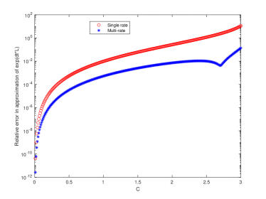
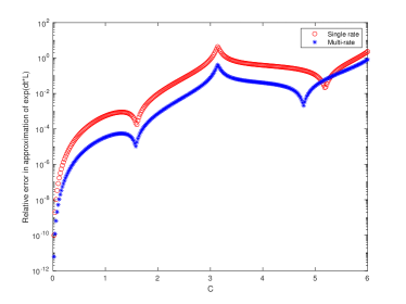
a) b)

Figure 1: Errors with respect of exact solution at increasing values of $C$ for a) explicit fourth order RK method, b) ESDIRK fourth order method.

5 Numerical results

The multi-rate Runge-Kutta methods presented in the previous Sections were implemented in the GBODE solver of the open-source OpenModelica simulation environment [6]. OpenModelica allows to model and simulate dynamical systems described by differential-algebraic equations using the high-level, equation-based, object-oriented modelling language Modelica [14]. OpenModelica applies structural analysis, symbolic manipulation and numerical solvers to reduce the (possibly high-index) differential-algebraic formulation to a set of explicit ordinary differential equations, producing efficient C code to compute the right-hand-side of Equation (1.1), which is then linked to the numerical solver GBDODE.

The implementation of the multi-rate method in GBODE is quite efficient from a computational point of view, as it was written using the C language and sparse linear algebra solvers for the implicit methods. It also supports dense output to provide the solution on a regular time grid, which was actually used to produce the numerical results shown in this Section, as well as to compute accurate high-order interpolation of slow variables during refinement steps.

Unfortunately, OpenModelica is presently not yet capable to produce code that selectively computes only the sub-set of fast variable right hand sides $f_{f}(y_{s},y_{f},t)$ in Equation (1.1). As a consequence, it will always compute the entire vector $f(y,t)$ also when performing the refinement steps, thus losing one of the main advantages of multi-rate methods. Hence, it is currently not possible to demonstrate a significant CPU time speed-up of the multi-rate methods, compared to the single-rate ones.

However, it is still possible to show that the number of right hand side computations actually needed by the multi-rate method is substantially reduced, compared to the standard single-rate method, while still providing an accurate solution. This demonstrates the soundness and applicability of the proposed multi-rate methods to real-life problems and gives a strong indication that the actual computational time will also be substantially reduced, once the selective computation feature is also implemented.

In the next sub-sections, three numerical test cases are presented, reporting results with the multi-rate versions of the methods fully described in Appendix A. The numerical results demonstrate how the proposed multi-rate method works when simulating non-trivial systems. Although OpenModelica is capable of handling extremely complex dynamical system models, for this paper we have selected test cases whose model equations can be written explicitly, so that the results are in principle reproducible with other implementations of the multi-rate method or different numerical approaches.

5.1 Inverter Chain

The first test case consists of the model of an inverter chain, which is an important test problem for electrical circuits that has already been considered in the literature on multi-rate methods, e.g., in [21, 22]. The system of equations is given by

$$y^{\prime}_{1}(t)=U_{op}-y_{1}(t)-\Gamma g(u(t),y_{1}(t))$$ (5.1)

$$y^{\prime}_{j}(t)=U_{op}-y_{j}(t)-\Gamma g(y_{j-1}(t),y_{j}(t)),\quad j=2,3,...,N,$$ (5.2)

where $y_{j}$ is the output voltage of the $j$-th inverter, $u(t)$ is the input voltage of the first inverter, $U_{op}$ is the operating voltage corresponding to the logical value 1, and $\Gamma$ is a stiffness parameter. The function $g$ is defined as

$$g(y,z)=\max(y-U_{\tau},0)^{2}-\max(y-z-U_{\tau})^{2},$$ (5.3)

where $U_{\tau}$ is a switching threshold. The system has a stable equilibrium if the input is zero, the odd-numbered inverters have output zero and the even-numbered inverters have output one. If the input is increased up to $U_{op}$, the first inverter output switches from zero to one, triggering a switching cascade that propagates through the entire chain at finite speed. If the first inverter input is then switched back to zero, a second switching cascade will propagate again through the system, bringing it back to the original equilibrium. This problem is obviously a good candidate for adaptive multi-rate integration, since only a small fraction of inverter outputs are changing at any given time. It is also representative of the simulation of real-life electronic digital circuit models, where only a small fraction of gates is active at any given point in time, while most other gates sit idle in a stable state.

The model was set up with $N=1000$ inverters, $U_{op}=5$, $U_{\tau}=1$, and $\Gamma=500$. The integration interval is $t\in[0,200]$, with initial conditions $y_{j}(0)=6.247\times 10^{-3}$ for even $j$ and $y_{j}(0)=1$ for odd $j$; $u(t)$ is a continuous piecewise-linear function which is zero until $t=5$, then increases to 5 until $t=10$, remains constant until $t=15$, decreases to zero until $t=20$ and then remains zero for $t>20$. We have used the third order ESDIRK method denoted as ESDIRK3(2)4L[2]SA in [11] to compute a reference single-rate solution with relative and absolute tolerance $10^{-9},$ a single-rate solution with relative and absolute tolerance $10^{-5}$ and multi-rate solution with relative and absolute tolerance $10^{-5}$. For the multi-rate algorithms, the parameter values $\alpha_{max}=1.2$, $\alpha_{min}=0.5$, $\alpha=0.9$, $\phi=0.05$, and $\beta=1$ were used; the associated dense output reconstruction was used for the interpolation operator $Q(\tau)$, both in the multi-rate procedure to interpolate the slow variables when integrating the fast variables, and when re-sampling the solution over a regular time grid with 0.01 s intervals.

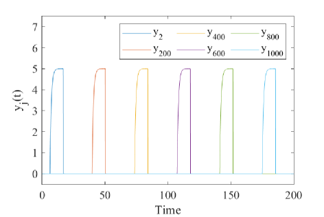
Figure 2: Reference solution for selected even inverter outputs.

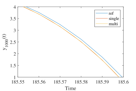
Figure 3: Comparison of reference, single-rate, and multi-rate ESDIRK3(2)4L[2]SA solutions in the inverter test case.

Figure 2 shows the output of the even inverters $y_{200},$ $y_{400},$ $y_{600},$ $y_{800},$ $y_{1000}$ in the reference solution, which follow the rising and falling edges of the first even inverter output $y_{2}$ with increasing delay, corresponding to about 150 time units for the last inverter output $y_{1000}$. Figure 3 shows a detail of the falling edge of the last inverter output $y_{1000}$, comparing the reference, single-rate, and multi-rate solutions: it is apparent how the multi-rate solution is virtually identical to the single-rate one, and that both are shifted in time with respect to the reference one by about 0.0015 time units, a relative error of $10^{-5}$, which is compatible with the tolerances employed.

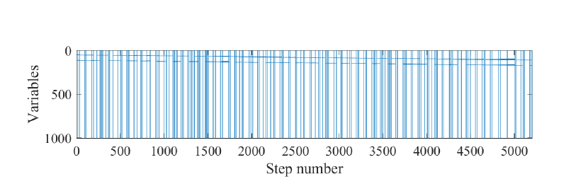
Figure 4: Activity diagram of the ESDIRK3(2)4L[2]SA multi-rate solution in the inverter test case.

Figure 4 shows the activity diagram of the multi-rate algorithm between $t=25$ and $t=35$. Here, the rows correspond to the variables in vector $y$, while the columns correspond to time steps; blue points correspond to variables that are active in a given time step. The full blue vertical lines correspond to global time steps, where all variables are involved in the computation of the time step, while the slightly slanted pairs of horizontal blue segments correspond to the rising and falling inverter output waves, slowly moving along the inverter chain. Only the inverters currently undergoing the transition are automatically selected as active variables during refinement steps. The activity plots clearly highlights the ability of the self-adjusting multi-rate approach to identify automatically the set fast evolving variables, which is essential if this set is time-varying.

In this specific example, the activity of fast states is quite localized: the typical size of the fast variable subspace is about 5, i.e., $1/200$ of the global system size $N.$ This means that, as long as $\phi$ is significantly less than one (otherwise most steps would be chosen as global ones), and larger than $1/200$, the same number of fast states will be selected. This was experimentally confirmed by running the simulations with different values of $\phi$ in the range $0.4<\phi<0.01$, which led to very similar results in terms of number of global and refinement steps. In general, the performance of the proposed multi-rate algorithm will not be too sensitive to the specific value of $\phi$ for those cases where the multi-rate strategy is more advantageous, i.e., when there is strongly localized activity most of the time, so that only a tiny fraction of variables shows significant integration errors for most of the time steps.

	Single-Rate	Multi-Rate
Total steps	77322	87803
Accepted global steps	65263	3201
Rejected global steps	12059	820
Accepted fast steps	//	73161
Rejected fast steps	//	10621
Total # of DOF	$7.73\times 10^{7}$	$4.30\times 10^{6}$

Table 9: Performance of single- and multi-rate ESDIRK3(2)4L[2]SA methods in the inverter test case.

Finally, Table 9 shows the comparison of some performance indicators of the single and multi-rate algorithms. The multi-rate method needs a total number of steps which is comparable to that of the single-rate method, but it requires one order of magnitude less global steps, while most of fast multi-rate steps involve a very small number of variables. As a consequence, the total number of DOF involved in all the steps of the multi-rate method is also one order of magnitude smaller, leading to a correspondingly lower computational workload for the computation of the elements in the right-hand-side of Equation (1.1).

5.2 Finite difference discretization of the Burgers equation

The second test case consists of an application to a PDE problem. We consider the viscous Burgers equation

$$\frac{\partial u}{\partial t}+u\frac{\partial u}{\partial x}=\nu\frac{\partial^{2}u}{\partial x^{2}}$$ (5.4)

as a simple model of computational fluid dynamics applications. The equation is considered on the domain $[0,25]$ and time interval $[0,5].$ We assume $\nu=10^{-2}$ and an initial datum given by

$$u_{0}(x)=\exp\left\{-\left(\frac{x-L/2}{L/50}\right)^{2}\right\}.$$ (5.5)

Equation (5.4) is semi-discretized in space by a standard centered finite difference approximation on a uniform mesh on $[0,25]$ with $N=1000$ nodes. We used the third order ESDIRK method denoted as ESDIRK3(2)4L[2]SA in [11] to compute a reference single-rate solution with relative and absolute tolerance $10^{-8}$, a single-rate solution with relative and absolute tolerance $10^{-5}$, two multi-rate solutions with relative and absolute tolerance $10^{-5}$, one with $\phi=0.2$ and one with $\phi=0.04$, and another two multi-rate solutions with relative and absolute tolerance $10^{-6}$, one with $\phi=0.2$ and one with $\phi=0.04$. The associated dense output reconstruction was used for the interpolation operator $Q(\tau)$, both in the multi-rate procedure to interpolate the slow variables when integrating the fast variables, and when re-sampling the solution over a regular time grid with 0.1 s time intervals. For the multi-rate algorithms, the parameter values $\alpha_{max}=1.2$, $\alpha_{min}=0.5$, $\alpha=0.9$, and $\beta=1$ were used.

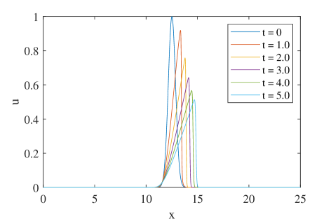
Figure 5: Reference solution for Burgers equation test case.

Fig. 5 shows the reference solution $u(x,t)$ along the spatial axis at five subsequent time instants. As time progresses, a sharp shock wave is formed on the right boundary of the active region, only slightly smoothed by the diffusion term, moving to the right at finite speed, followed by a trailing region where the values of $u$ slowly get back to zero. After $t=1$, for each time instant the variable vector can be partitioned in three subsets. One, involving a few percent of the node variables, corresponds to the fast-changing shock wave. The second, involving about 15% of the node variables, corresponds to the slow trailing wave, while the remaining part of the node vector contains values very close to zero.

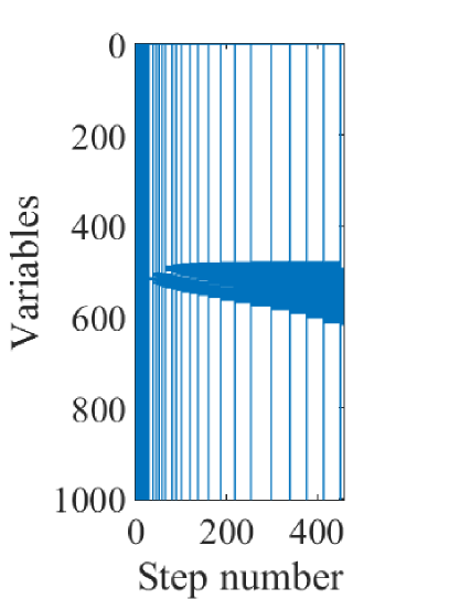
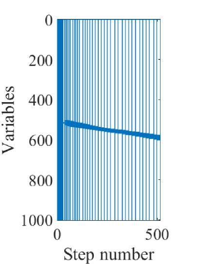
Figure 6: Activity diagram of Burgers’ equation test case, tolerance $10^{-5}$, left $\phi=0.2$, right $\phi=0.04$.

The activity diagram in the case $\phi=0.2$ is shown in the left half of Fig. 6. For this computation, relative and absolute tolerance values were set to $10^{-5}$. The fast variable subsets ${\cal V}^{f}_{n}$ encompass the first two above-mentioned subsets, where basically all the action takes place in the solution, corresponding to the central blue part of the diagram. After $t=1$, only a very few global steps, about one every 80 fast refinement steps, are taken to compute the components of the solution belonging to the third subset.

If a smaller value $\phi=0.04$ is chosen, the activity diagram shown in the right half of Fig. 6 is obtained. In this case, the sets ${\cal V}^{f}_{n}$ are too small to encompass the second subset. Instead, they only cover the much narrower subset of variables corresponding to the shock transition, moving from left to right, while the degrees of freedom corresponding to the trailing region and to the essentially constant part of the solution constitute the subset of slow variables. Therefore, compared to the previous solution, there are more global steps, but on the other hand the fast steps involve a much smaller set of variables.

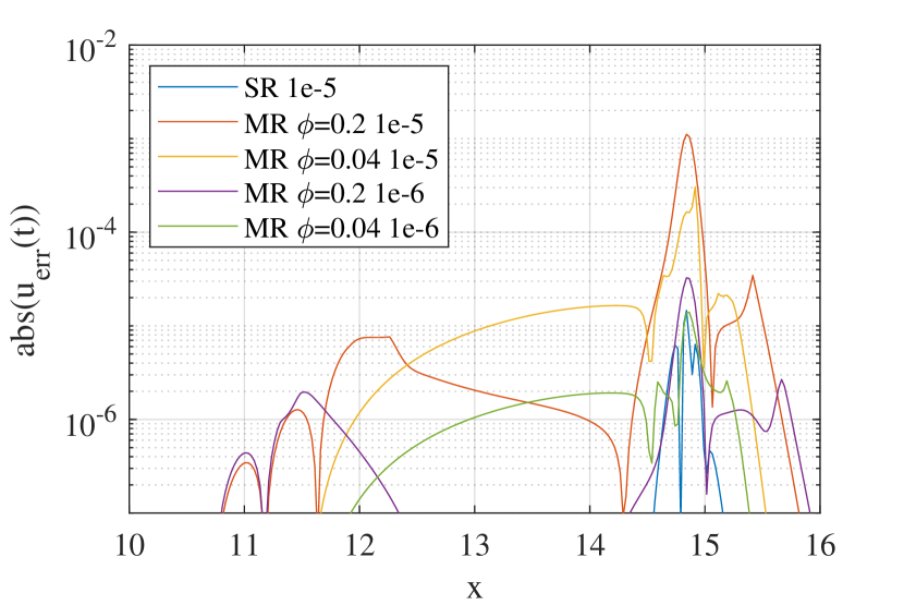
Figure 7: Absolute error for the solution of Burgers equation.

Fig. 7 shows the spatial distribution of the absolute error over the spatial domain at $t=5$. The error is computed considering the difference between the single-rate and multi-rate solutions and the reference solution computed with the single rate method employed with tolerance $10^{-8}$. It is to be remarked that, in this way, only an estimate of the time discretization error is obtained, since all methods use the same spatial discretization. The interaction of time and space discretization errors is an extremely important point for application to PDE solvers, which is however beyond the scope of this work. For the single-rate solution with tolerance $10^{-5}$, the maximum error is about $1.5\cdot 10^{-5}$, which is consistent with the selected tolerance. The multi-rate solutions with tolerance $10^{-5}$ show a significantly larger error around $x=14.8$, where the steepest region of the shock wave is located, with maximum errors of about $3\cdot 10^{-4}$ for $\phi=0.04$ and $10^{-3}$ for $\phi=0.02$. Maximum errors around $10^{-5}$ can also be obtained with the multi-rate algorithms by reducing the tolerance to $10^{-6}$.

Finally, Table 10 compares the performance of the single- and multi-rate simulations. For this test case, the number of total degrees of freedom involved in the computation is reduced by a about a factor four if the same tolerance is kept, or by about a factor three if the same accuracy is kept.

	SR	MR	MR	MR	MR
		$\phi=0.2$	$\phi=0.2$	$\phi=0.04$	$\phi=0.04$
		$tol=10^{-5}$	$tol=10^{-6}$	$tol=10^{-5}$	$tol=10^{-6}$
Total steps	383	457	937	515	1142
Accepted global steps	383	49	56	67	112
Rejected global steps	0	0	0	0	0
Accepted fast steps	//	408	881	448	1030
Rejected fast steps	//	0	0	0	0
Total # of DOF	383000	85996	150542	76865	134453

Table 10: Performance of single- and multi-rate ESDIRK3(2)4L[2]SA methods on Burgers’ equation test case.

5.3 Thermal model of a large building heating system

The third test case consists of an idealized model of the thermal behaviour of a large building with $N=100$ heated units. For simplicity, it is assumed that each unit, with temperature $T_{u,j},$ is well-insulated from the others and only interacts with a central heating system with supply temperature $T_{s}$ and with the external environment at temperature $T_{e}$, which is assumed to vary sinusoidally during the day with a peak at 14:00. The thermal supply system has a temperature $T_{s}$, which is regulated by a proportional controller with fixed set point $T_{s}^{0}$, that acts on the heat input $Q_{s}$. The total energy consumption of the thermal supply system is tracked by the variable $E$.

Each unit has a proportional temperature controller with variable set point $T_{u,j}$, acting on the command signal $u_{j}$ of a heating unit with thermal conductance $G_{h}$ (e.g., a fan coil with variable fan speed), which responds to the command as a first-order linear system with time constant $t_{h}$. The heating unit then enables the heat transfer between the heating fluid of the supply system and the room, with thermal power $Q_{h,j}$. Each unit also exchanges a thermal power $Q_{e,j}$ with the external environment.

The model is described by the following system of differential-algebraic equations:

$$T_{e}=278.15+8\cos\left(2\pi\frac{t-14\times 3600}{24\times 3600}\right)$$ (5.6)

$$Q_{s}=sat(K_{ps}Q_{max}(T_{s}^{0}-T_{s}),0,Q_{max})$$ (5.7)

$$Q_{ht}=\sum_{1}^{N}{Q_{h,j}}$$ (5.8)

$$C_{s}\frac{dT_{s}}{dt}=Q_{s}-Q_{ht}$$ (5.9)

$$t_{h}\frac{dG_{h,j}}{dt}=u_{j}G_{hn}-G_{h,j}, \quad j=1,...,N$$ (5.10)

$$Q_{h,j}=G_{h,j}(T_{s}-T_{u,j}), \quad j=1,...,N$$ (5.11)

$$Q_{e,j}=G_{u}(T_{u,j}-T_{e}), \quad j=1,...,N$$ (5.12)

$$C_{u,j}\frac{dT_{u,j}}{dt}=Q_{h,j}-Q_{e,j}, \quad j=1,...,N$$ (5.13)

$$u_{j}=sat(K_{pu}(T^{0}_{u,j}-T_{u,j}),0,1), \quad j=1,...,N$$ (5.14)

$$T^{0}_{u,j}=f_{j}(t), \quad j=1,...,N$$ (5.15)

$$\frac{dE}{dt}=Q_{s}$$ (5.16)

which can be easily reformulated by substitution as a system of $2N+2$ ordinary differential equations in the variables $T_{s}$, $G_{h,j}$, $T_{u,j}$, and $E$.

We assume the following values for the system parameters: $K_{ps}=0.2$, $T_{h}=293.15$, $T_{l}=288.15$, $T^{0}_{s}=343.15$, $G_{hn}=200$, $G_{u}=150$, $Q_{max}=0.7NG_{hn}(T^{0}_{s}-T_{h})$, $C_{s}=2\cdot 10^{6}N$, $t_{h}=20$, $C_{u,j}=(1+0.348j/N)\times 10^{7}$, $K_{pu}=1$. All the values of physical constants are in SI units.

The functions $f_{j}(t)$ are periodic with a period of one day, i.e., 86400 s. They start at $T_{l}$ at midnight, get increased from $T_{l}$ to $T_{h}$ at a pseudo-random time between 6 and 12 am, and switch back to $T_{l}$ at a pseudo-random time between 15 and 22 pm. The transitions are smooth, using the $smoothStep(\cdot,\cdot,\cdot)$ function defined as

$$smoothStep(t,t_{s},\Delta t)=\frac{1}{2}\left(\tanh\left(\frac{t-t_{s}}{\Delta t}\right)+1\right),$$ (5.17)

with $\Delta t=1$ s, while the function $sat(\cdot,\cdot,\cdot)$ is a smooth saturation function defined as

$$sat(x,x_{min},x_{max}) = \frac{x_{max}+x_{min}}{2}$$

$$+ \frac{x_{max}-x_{min}}{2}\tanh\left(2\frac{x-x_{min}}{x_{max}-x_{min}}-1\right).$$

The initial conditions of the system at $t=0$ (corresponding to 00:00, midnight) are $T_{s}=T^{0}_{s}$, $G_{h,j}=0$, $T_{u,j}=288.15$, $E=0$. The integration interval is two days, i.e $t\in\left[0,172800\right]$.

We have used the fourth order ESDIRK method denoted as ESDIRK4(3)6L[2]SA in [11] to compute a reference single-rate solution with relative and absolute tolerance $10^{-9},$ a single-rate solution with relative and absolute tolerance $10^{-5}$ and multi-rate solution with relative and absolute tolerance $10^{-5}$. For the multi-rate algorithms, the parameter values $\alpha_{max}=1.2$, $\alpha_{min}=0.5$, $\alpha=0.9$, $\phi=0.05$, and $\beta=1$ were used; the associated dense output reconstruction was used for the interpolation operator $Q(\tau)$, both in the multi-rate procedure to interpolate the slow variables when integrating the fast variables, and when re-sampling the solution over a regular time grid with 10 s intervals.

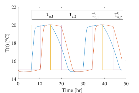
Figure 8: Temperatures and set points for units 1 and 2.

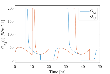
Figure 9: Conductance of fan-coils of units 1 and 2.

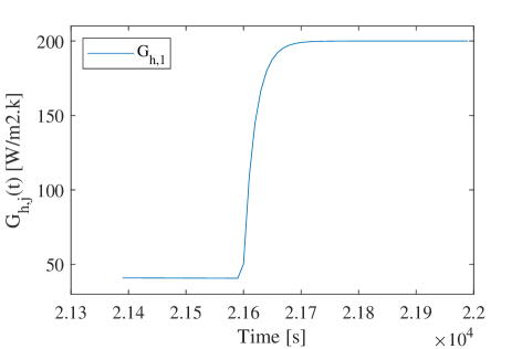
Figure 10: Detail of the first rising front of fan-coil 1.

Figure 8 shows the temperatures and the respective set points for units 1 and 2. The set point for the first unit $T^{0}_{u,1}$ is raised around 6:00 and reduced around 14:00, while the set point for the second unit $T^{0}_{u,1}$ is raised around 10:00 and reduced around 20:00. The unit temperatures $T_{u,1}$ and $T_{u,2}$ follow with some delay. Falling temperature transients are slower because they are only driven by the heat losses to the ambient.

Figure 9 shows the fan-coil conductances $G_{h,1}$ and $G_{h,2}$. Initially, they are quite low, to keep the night temperature around $T_{l}.$ Subsequently, they very quickly reach the maximum value when the set point is raised, remain at the maximum for a while and then decrease once the unit temperatures approach the new set point value $T_{h}$, and drop sharply to zero when the set point is reduced to $T_{l}$ in the afternoon, increasing again during the night once the temperature has fallen below the set point. The dynamics of $G_{h,1}$ is much faster than the dynamics of the temperatures, see the detail of the first rising front of $G_{h,1}$ shown in Figure 10.

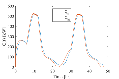
Figure 11: Input and output thermal power of the supply system.

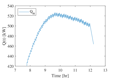
Figure 12: Zoom-in of the total output thermal power of the supply system between 7:45 and 12:15 on day 1.

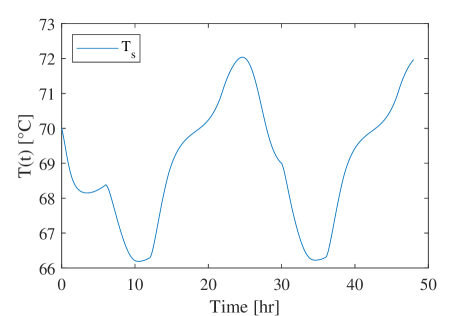
Figure 13: Heating supply temperature.

Figure 11 shows the thermal power input of the supply system $Q_{s}$ and the total thermal power output to the unit fan coils $Q_{ht}$, with a zoom-in of $Q_{ht}$ between 7:45 and 12:15 shown in Figure 12. The supply temperature $T_{s}$ is shown in Figure 13.

The reason why this system can benefit from multi-rate integration is twofold: the various occupants change their unit set points asynchronously, and the changes applied to one unit are very weakly coupled to the other units through the large thermal inertia of the supply system. Every time an occupant gets to its unit and raises the set point in the morning, or reduces it in the evening, a local fast transient is triggered on the unit’s temperature control system output $u_{j}$, which requires relatively short time steps to simulate the transient of $G_{h,j}.$ However, this action does not influence the other units directly, because they are insulated from each other, but rather only through the increased or decreased power consumption $Q_{ht}$, shown in Figure 11. Even though $Q_{ht}$ shows fast changes, see Fig. 12, corresponding to the individual unit heating systems being turned on or off, the large inertia of the supply system causes the supply temperature $T_{s}$ to remain quite smooth, as shown in Figure 13, so that the influence of these events on the heat exchanged by the other units becomes relevant only over much larger time intervals, even more so as $N$ grows.

Hence, every set point switching transient can be handled by a set of fast variables that only includes the local heater conductance $G_{h,j}$, the unit temperature $T_{u,j}$, the supply temperature $T_{s}$, and the consumed energy $E$, using interpolated values for the other unit variables, $G_{h,k},T_{u,k},k\neq j$, which only start getting influenced by the consequences of switching in other units after hundreds of seconds. This brings down the number of DOF required to manage these transients from $2N+2$ to $O(1)$.

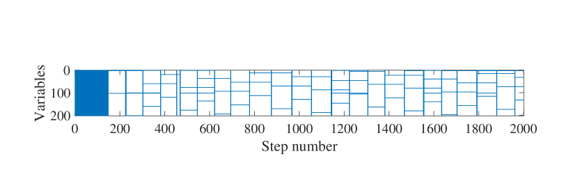
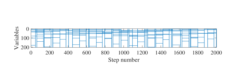
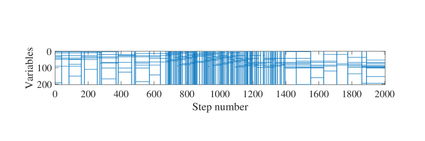
Figure 14: Activity diagrams of the multi-rate solution.

Figure 14 shows three portions of the activity diagram, with rows corresponding to variables and columns to time steps. The top diagram corresponds to the beginning of the simulation, from 00:00 to 07:30. The first 145 steps to the left of the diagram correspond to the night transient from 00:00 to 06:00. During this period, no set points are changed, so there are no fast local transients taking place in the system, only the response of all the system variables to the slow sinusoidal variation of the external ambient temperature, which is handled by global time steps up to 1200 s long.

After 06:00, the unit temperature set points start being increased from $T_{l}$ to $T_{h}$, in a pseudo-random fashion, triggering many local fast transient. As a consequence, the average step length is dramatically reduced, and the remaining portion of the topmost activity diagram, spanning until 07:30, shows a very sparse pattern, where the two bordering lines at the top and bottom correspond to $T_{u}$ and $E$, which are always active, while the other shorter horizontal segments correspond to the transients of $G_{h,j}$ and $T_{u,j}$, which are handled by fast refinement steps; only a few global steps are necessary, shown in the figure as vertical blue bands).

This pattern continues until 12:00, e.g., see the the middle diagram of Figure 14, covering the time interval from 8:45 to 10:00.

The bottom diagram of Figure 14, which covers the interval from 11:30 to 15:30, shows the sparse patterns ending at 12:00, when set points stop being changed, followed by a pattern composed of mostly global steps until between 12:00 and 15:00, when the room temperatures mostly react to the slowly changing external temperature, after which set points start changing again, bringing the sparse pattern in again, and so on.

The most important result of this simulation is the final value of the energy consumption $E$, reported in Table 11 for the three solutions. The multi-rate result is affected by a larger error than the single-rate one, but it still has 5 correct significant digits, which is in agreement with the set relative and absolute tolerances $10^{-5}$.

	Total Consumption [MWh]
Reference	10.16868431299
Single-Rate	10.16868431246
Multi-Rate	10.16803623248

Table 11: Total energy consumption computed by the ESDIRK4(3)6L[2]SA method.

	Single-Rate	Multi-Rate
Total steps	33575	37824
Accepted global steps	27644	1107
Rejected global steps	5931	79
Accepted fast steps	//	30970
Rejected fast steps	//	5668
Total # of DOF	$6.78\times 10^{6}$	$0.47\times 10^{6}$

Table 12: Performance of single- and multi-rate ESDIRK4(3)6L[2]SA method.

The performance comparison between the single-rate and the multi-rate ESDIRK4(3)6L[2]SA method is shown in Table 12. As in the previous case, the number of total time steps required by the multi-rate method is similar to that of the single-rate method, but the number of global steps is more than one order of magnitude smaller, and so is the total number of active variables at each time step.

6 Conclusions and future work

We have presented a more general and effective version of the self-adjusting multi-rate procedure already introduced in [5]. The novel approach allows to obtain a more effective multi-rate implementation of a generic Runge-Kutta (RK) method by combining a self-adjusting multi-rate technique with standard time step adaptation methods. Only a small percentage of the variables, associated with the largest values of an error estimator are marked as fast variables. When the global step is sufficient to guarantee a given error tolerance for the slow variables, but not for the fast ones, the multi-rate procedure is employed to achieve uniform accuracy at reduced computational cost.

We have also provided a general stability analysis, valid for explicit RK, DIRK and ESDIRK multi-rate method with an arbitrary number of sub-steps for the active components. We have proposed a physically motivated model problem that can be used to assess the stability of different multi-rate versions of standard RK methods and the impact of different interpolation methods for the latent variables. The stability analysis has been performed on some examples of ERK and ESDIRK methods, highlighting the potential gains in efficiency and accuracy that can be achieved by the multi-rate approach in the regime of weak coupling between fast and slow variables.

The proposed multi-rate methods have then been applied to three numerical benchmarks, representing two idealized engineering systems and a basic discretization of a nonlinear PDE typical of Computational Fluid Dynamics applications. The simulations have been performed using an implementation of the proposed multi-rate approach in the framework of the OpenModelica software [6]. The results demonstrate the efficiency gains deriving from the use of the proposed multi-rate approach for problems with multiple time scales.

In future work, we will further pursue the application of this kind of multi-rate methods to the time discretization of partial differential equations, already started in [5], along with a more effective OpenModelica implementation that will allow to reap the full benefit of the multi-rate approach by avoiding unnecessary computation of the slow components during fast steps.

Appendix A Butcher tableaux of RK methods

For completeness, we report in this Appendix the Butcher tableaux of the methods considered in the stability analysis, along with the coefficients of their corresponding dense output interpolators. Table 13 contains the coefficients defining the classical fourth order explicit RK method. Table 14 contains the coefficients defining the fourth order RK method with optimal continuous output introduced in [17]. The matrix $B^{*}$ containing the coefficients for the dense output formula (3) associated to this method are given in Table 15. Setting then

$$\gamma = 0.43586652150845899941601945,$$

$$c_{3} = \frac{3}{5},\ \ \ \ \bar{a}=1-6\gamma+6\gamma^{2}$$

$$a_{32} = c_{3}\frac{c_{3}-2\gamma}{4\gamma}\ \ \ a_{31}=c_{3}-a_{32}-\gamma$$ (A.1)

$$b_{2} = \frac{-2+3c_{3}+6\gamma(1-c_{3})}{12\gamma(c_{3}-2\gamma)}\ \ \ b_{3}=\frac{\bar{a}}{3c_{3}(c_{3}-2\gamma)}$$

$$b1 = 1-b2-b3-\gamma,$$

we report in Table 16 the coefficients of the third order ESDIRK method denoted as ESDIRK3(2)4L[2]SA in [11]. The corresponding matrix $B^{*}$ containing the coefficients for the dense output formula (3) are given in Table 17.

0	0	0	0	0
$\frac{1}{2}$	$\frac{1}{2}$	0	0	0
$\frac{1}{2}$	$0$	$\frac{1}{2}$	0	0
$1$	$0$	$0$	1	0
	$\frac{1}{6}$	$\frac{2}{6}$	$\frac{2}{6}$	$\frac{1}{6}$

Table 13: Butcher tableaux of the classical fourth order ERK method.

0	0	0	0	0	0	0
$\frac{1}{6}$	$\frac{1}{6}$	0	0	0	0	0
$\frac{11}{37}$	$\frac{44}{1369}$	$\frac{363}{1369}$	0	0	0	0
$\frac{11}{17}$	$\frac{3388}{4913}$	$-\frac{8349}{4913}$	$-\frac{8140}{4913}$	0		0
$\frac{13}{15}$	$-\frac{36764}{408375}$	$\frac{767}{1125}$	$-\frac{32708}{136125}$	$\frac{210392}{408375}$	0	0
$1$	$\frac{1697}{18876}$	$0$	$\frac{50653}{116160}$	$\frac{299693}{1626240}$	$\frac{3375}{11648}$	0
	$\frac{101}{363}$	$0$	$-\frac{1369}{14520}$	$\frac{11849}{14520}$	0	0

Table 14: Butcher tableaux of optimal explicit RK method with continuous output.

$b^{*}_{ij}$	$j=1$	$j=2$	$j=3$	$j=4$
$i=1$	$1$	$-\frac{104217}{37466}$	$\frac{1806901}{618189}$	$-\frac{866577}{824252}$
$i=2$	$0$	$0$	$0$	0
$i=3$	$0$	$\frac{861101}{230560}$	$-\frac{2178079}{380424}$	$\frac{12308679}{5072320}$
$i=4$	$0$	$-\frac{63869}{293440}$	$\frac{6244423}{5325936}$	$-\frac{7816583}{10144640}$
$i=5$	$0$	$-\frac{1522125}{762944}$	$\frac{982125}{190736}$	$-\frac{624375}{217984}$
$i=6$	$0$	$\frac{165}{131}$	$-\frac{461}{131}$	$\frac{296}{131}$

Table 15: Matrix of continuous output coefficients $b^{*}_{ij}$ for explicit RK method of [17].

0	0	0	0	0
$2\gamma$	$\gamma$	$\gamma$	0	0
$\frac{3}{5}$	$a_{31}$	$a_{32}$	$\gamma$	0
$1$	$b_{1}$	$b_{2}$	$b_{3}$	$\gamma$
	$b_{1}$	$b_{2}$	$b_{3}$	$\gamma$

Table 16: Butcher tableaux of the ESDIRK3(2)4L[2]SA method.

$b^{*}_{ij}$	$j=1$	$j=2$	$j=3$
$i=1$	$\frac{6071615849858}{5506968783323}$	$-\frac{9135504192562}{5563158936341}$	$\frac{5884850621193}{8091909798020}$
$i=2$	$\frac{24823866123060}{14064067831369}$	$-\frac{184358657789355}{34679930461469}$	$\frac{40093531604824}{13565043189019}$
$i=3$	$-\frac{4639021340861}{5641321412596}$	$-\frac{36951656213070}{8103384546449}$	$-\frac{9445293799577}{3414897167914}$
$i=4$	$-\frac{4782987747279}{4575882152666}$	$\frac{22547150295437}{9402010570133}$	$-\frac{8621837051676}{9402290144509}$

Table 17: Matrix of continuous output coefficients $b^{*}_{ij}$ for the ESDIRK3(2)4L[2]SA method.

0	0	0	0	0	0	0
$2\gamma$	$\gamma$	$\gamma$	0	0	0	0
$c_{3}$	$a_{31}$	$a_{32}$	$\gamma$	0	0	0
$c_{4}$	$a_{41}$	$a_{42}$	$a_{43}$	$\gamma$	0	0
$c_{5}$	$a_{51}$	$a_{52}$	$a_{53}$	$a_{54}$	$\gamma$	0
$1$	$b_{1}$	$b_{2}$	$b_{3}$	$b_{4}$	$b_{5}$	$\gamma$
	$b_{1}$	$b_{2}$	$b_{3}$	$b_{4}$	$b_{5}$	$\gamma$

Table 18: Butcher tableaux of the ESDIRK4(3)6L[2]SA method.

Table 18 contains instead the coefficients defining the fourth order ESDIRK method denoted as ESDIRK4(3)6L[2]SA in [11], where we have set instead

$$\gamma = 1/4c_{3}=\frac{2-\sqrt{2}}{4}\ \ \ \ c_{4}=\frac{5}{8}\ \ c_{5}=\frac{26}{25}$$

$$a_{32} = \frac{1-\sqrt{2}}{8}\ \ a_{31}=c_{3}-a_{32}-\gamma$$

$$a_{42} = \frac{5-7\sqrt{2}}{64}\ \ \ \ a_{43}=7\frac{1+\sqrt{2}}{32}\ \ \ \ a_{41}=c_{4}-a_{42}-a_{43}-\gamma$$

$$a_{52} = \frac{-13796-54539\sqrt{2}}{125000}\ \ a_{53}=\frac{506605+132109\sqrt{2}}{437500}$$ (A.2)

$$a_{54} = 166\frac{-97+376\sqrt{2}}{109375}\ \ a_{51}=c_{5}-a_{52}-a_{53}-a_{54}-\gamma$$

$$b_{2} = \frac{1181-987\sqrt{2}}{13782}\ \ \ \ b_{3}=47\frac{(-267+1783\sqrt{2}}{273343}$$

$$b_{4} = -16\frac{-22922+3525\sqrt{2}}{571953}\ \ \ \ b_{5}=-15625\frac{97+376\sqrt{2}}{90749876}$$

$$b_{1} = 1-b_{2}-b_{3}-b_{4}-b_{5}-\gamma.$$

The corresponding matrix $B^{*}$ containing the coefficients for the dense output formula (3) are given in Table 19.

$b^{*}_{ij}$	$j=1$	$j=2$	$j=3$	$j=4$
$i=1$	$\frac{11963910384665}{12483345430363}$	$-\frac{69996760330788}{18526599551455}$	$\frac{32473635429419}{7030701510665}$	$-\frac{14668528638623}{8083464301755}$
$i=2$	$\frac{11963910384665}{12483345430363}$	$-\frac{69996760330788}{18526599551455}$	$\frac{32473635429419}{7030701510665}$	$-\frac{14668528638623}{8083464301755}$
$i=3$	$-\frac{28603264624}{1970169629981}$	$\frac{102610171905103}{26266659717953}$	$-\frac{38866317253841}{6249835826165}$	$\frac{21103455885091}{7774428730952}$
$i=4$	$-\frac{3524425447183}{2683177070205}$	$\frac{74957623907620}{12279805097313}$	$-\frac{26705717223886}{4265677133337}$	$\frac{30155591475533}{15293695940061}$
$i=5$	$-\frac{17173522440186}{10195024317061}$	$\frac{113853199235633}{9983266320290}$	$-\frac{121105382143155}{6658412667527}$	$\frac{119853375102088}{14336240079991}$
$i=6$	$\frac{27308879169709}{13030500014233}$	$-\frac{84229392543950}{6077740599399}$	$\frac{1102028547503824}{51424476870755}$	$-\frac{63602213973224}{6753880425717}$

Table 19: Matrix of continous output coefficients $b^{*}_{ij}$ for the ESDIRK4(3)6L[2]SA method.

References

- [1] J.F. Andrus. Numerical solution of systems of ordinary differential equations separated into subsystems. SIAM Journal of Numerical Analysis, 16:605–611, 1979.
- [2] D. Arndt, W. Bangerth, M. Feder, M. Fehling, R. Gassmöller, T. Heister, L. Heltai, M. Kronbichler, M. Maier, P. Munch, J.-P. Pelteret, S. Sticko, B. Turcksin, and D. Wells. The deal II library, version 9.4. Journal of Numerical Mathematics, 30(3):231–246, 2022.
- [3] W. Bangerth, R. Hartmann, and G. Kanschat. deal II: a general-purpose object-oriented finite element library. ACM Transactions on Mathematical Software, 33:24–51, 2007.
- [4] R.E. Bank, W.M. Coughran, W. Fichtner, E.H. Grosse, D.J. Rose, and R.K. Smith. Transient simulation of silicon devices and circuits. IEEE Transactions on Electron Devices, 32:1992–2007, 1985.
- [5] L. Bonaventura, F. Casella, L. Delpopolo Carciopolo, and A. Ranade. A self adjusting multirate algorithm for robust time discretization of partial differential equations. Computers and Mathematics with Applications, 79:2086–2098, 2020.
- [6] P. Fritzson, A.Pop, K. Abdelhak, A. Ashgar, B. Bachmann, W.Braun, D.Bouskela, R. Braun, L. Buffoni, F. Casella, R. Castro, R. Franke, D. Fritzson, M. Gebremedhin, A. Heuermann, B. Lie, A. Mengist, L. Mikelsons, K. Moudgalya, L. Ochel, A. Palanisamy, V. Ruge, W. Schamai, M. Sjölund, B. Thiele, J. Tinnerholm, and P. Östlund. The OpenModelica Integrated Environment for Modeling, Simulation, and Model-Based Development. Modeling, Identification and Control, 41:241–295, 2020.
- [7] C.W. Gear and D.R. Wells. Multirate linear multistep methods. BIT Numerical Mathematics, 24:484–502, 1984.
- [8] E. Hairer, S.P. Nørsett, and G. Wanner. Solving Ordinary Differential Equations I Nonstiff problems. Springer, Berlin, second edition, 2000.
- [9] M.E. Hosea and L.F. Shampine. Analysis and implementation of TR-BDF2. Applied Numerical Mathematics, 20:21–37, 1996.
- [10] W. Hundsdorfer and V. Savcenco. Analysis of a multirate theta-method for stiff ODEs. Applied Numerical Mathematics, 59:693–706, 2009.
- [11] C. A. Kennedy and M.H. Carpenter. Diagonally implicit Runge-Kutta methods for ordinary differential equations, a review. Technical Report TM-2016-219173, NASA, 2016.
- [12] C. A. Kennedy and M.H. Carpenter. Diagonally implicit Runge-Kutta methods for stiff ODEs. Applied Numerical Mathematics, 146:221–244, 2019.
- [13] K. Kuhn and J. Lang. Comparison of the asymptotic stability for multirate Rosenbrock methods. Journal of Computational and Applied Mathematics, 262:139–149, 2014.
- [14] S. E. Mattsson, H. Elmqvist, and M. Otter. Physical system modeling with Modelica. Control Engineering Practice, 6(4):501–510, 1998.
- [15] G. Orlando, P. F. Barbante, and L. Bonaventura. An efficient IMEX-DG solver for the compressible Navier-Stokes equations for non-ideal gases. Journal of Computational Physics, 471:111653, 2022.
- [16] G. Orlando, A. Della Rocca, P. F. Barbante, L. Bonaventura, and N. Parolini. An efficient and accurate implicit DG solver for the incompressible Navier-Stokes equations. International Journal for Numerical Methods in Fluids, 94:1484–1516, 2022.
- [17] B. Owren and M. Zennaro. Derivation of efficient, continuous, explicit Runge–Kutta methods. SIAM Journal of Scientific and Statistical Computing, 13:1488–1501, 1992.
- [18] A. Quarteroni and A. Valli. Domain decomposition methods for partial differential equations. Oxford University Press, 1999.
- [19] J.R. Rice. Split Runge-Kutta methods for simultaneous equations. Journal of Research of the National Institute of Standards and Technology, 60, 1960.
- [20] V. Savcenco. Comparison of the asymptotic stability properties for two multirate strategies. Journal of Computational and Applied Mathematics, 220:508–524, 2008.
- [21] V. Savcenco, W. Hundsdorfer, and J.G. Verwer. A multirate time stepping strategy for stiff ordinary differential equations. BIT Numerical Mathematics, 47:137–155, 2007.
- [22] A. Verhoeven, B. Tasić, T.G.J. Beelen, E.J.W. ter Maten, and R.M.M. Mattheij. Automatic partitioning for multirate methods. In Scientific Computing in Electrical Engineering, pages 229–236. Springer, 2007.