Quantifying the Causal Effect of Financial Literacy Courses
on Financial Health

Abstract

In this study, we investigate the causal effect of financial literacy education on a composite financial health score constructed from 17 self-reported financial health and distress metrics ranging from spending habits to confidence in ability to repay debt to day-to-day financial skill. Leveraging data from the 2021 National Financial Capability Study, we find a significant and positive average treatment effect of financial literacy education on financial health. To test the robustness of this effect, we utilize a variety of causal estimators (Generalized Lin’s estimator, 1:1 propensity matching, IPW, and AIPW) and conduct sensitivity analysis using alternate health outcome scoring and varying caliper strengths. Our results are robust to these changes. The robust positive effect of financial literacy education on financial health found here motivates financial education for all individuals and holds implications for policymakers seeking to address the worsening debt problem in the U.S, though the relatively small magnitude of effect demands further research by experts in the domain of financial health.

1 Introduction

Consumer debt is widely understood to be a malignant and growing problem in the U.S. Measures of consumer debt are as high as they have ever been: Americans’ credit card debt recently crested over $1 trillion dollars for the first time, student loan debt now exceeds $1.7 trillion, and mortgage debt is over $20 trillion (Board of Governors of the Federal Reserve System (2023a), US; Board of Governors of the Federal Reserve System (2023c), US; Board of Governors of the Federal Reserve System (2023b), US). For young people in particular, debt is a severe problem; almost one in five age 18–24 Americans with a credit record have debt in collections (Martinchek et al., 2022).

An issue as pervasive and complex as mounting consumer debt fundamentally has many angles from which policymakers can attempt to address it. In this paper, we consider one popular method for reversing its growth: efforts to increase financial literacy. In an increasingly complex world where significant economic decisions are perpetually a click away in one’s pocket, it stands to reason that financial decision-making is as complicated as its ever been. Can financial literacy education then help people make sounder financial decisions? Many seem to think so. There are consistent calls for greater financial education for Americans (Washington Post Editorial Board, June 2022) (Kasman et al., 2018) (Stanford Institute for Economic Policy Research, 2023) and a number of states have enacted financial education requirements for high school students. In Tennessee, for example, completing a personal finance class has been a requirement for graduating high school since 2013 (Department of Financial Institutions, TN, 2013). In several more states, similar bills have already been voted through or taken effect (Ramsey Solutions, 2023). But do financial literacy classes really encourage better decisions and lead to better financial health?

In this analysis, we use the National Financial Capability Survey (NFCS) to assess the causal relationship between financial education and financial health outcomes. The primary analysis assesses the causal effect of financial literacy education on financial health outcomes, while the secondary analysis focuses more specifically on the effect of high-school based financial literacy education. Through this assessment, we hope to inform policymakers about financial education policies’ ability to positive impact Americans’ finances.

2 Related Work

The financial well-being of young Americans, and of college students in particular, has been studied extensively. Much existing research focuses on financial health in the context of student loans, and on the impact that debt repayment can have on financial independence. A study conducted by (Fan & Chatterjee, 2019) used the 2015 NFCS to examine the association of financial education and financial socialization with student loan repayments, but did not perform any causal analysis. Instead, it focused on associations between correct responses to financial knowledge questions, and whether individuals were on time with their student loan repayments.

Another study of the NFCS found that individuals with outstanding student loans were more likely to have other substantial debt obligations, such as credit card debt or car repayments (Fry, 2012). These findings were supported by more recent research (Lusardi & Mitchell, 2023), which indicated that areas with poor average financial literacy had higher wealth inequality, and that financial literacy metrics were heavily imbalanced across demographic categories such as race and age.

We seek to improve upon these studies by analyzing the impact of financial education across a more comprehensive outcome measure of financial health, and by employing robust causal frameworks to isolate the effect of financial education.

3 Data Features and Preprocessing

3.1 Data Source

In order to assess the effect of financial education on financial health outcomes, we used data downloaded from the National Financial Capability Study (NFCS) (FINRA Investor Education Foundation, 2023), commissioned by the FINRA Investor Education Foundation. The NFCS surveys a representative sample of approximately 500 people from each state, asking questions about their demographic background and level of education, and assessing their financial situation in terms of credit card debt, retirement savings, mortgage payments, and more. The survey began in 2009, and repeats every three years, with most recent data from 2021. For our study, we downloaded the 2021 archive of NFCS data. We opted not to include earlier data because many states implemented financial literacy laws for high school within the last ten years, and the 2021 dataset is recent enough to reflect those laws (Urban et al., 2020).

Two datasets were formed from the NFCS data. The primary dataset included participants who took a financial literacy course (treatment) in high-school, college, at work, or in the military, as well as participants who were certain they had never taken such a course (controls). Our second subset of data, designed for specifically analyzing the effect of high-school (HS) financial literacy education on financial health outcomes, includes participants who took a high-school financial literacy course, and participants who were sure they had not.

3.2 Data Cleaning

All data cleaning and feature engineering was performed using Python’s pandas library (McKinney, 2011). The associated data fact sheet for our downloaded 2021 NFCS data was used to derive a column map and rename columns to more appropriate and descriptive names. All strings were stripped of starting and trailing whitespace, string representations of integers were converted to integers, and NaN values were removed.

$17$ columns were identified as critical markers of financial health (see Appendix B). Given the inconsistency of the original answer choices for each survey question corresponding to these markers, results were scaled so that answer values ranged from $0$ to $9$ for all markers, with $0$ indicating poor relative financial health and $9$ indicating great relative financial health. In cases where the respondent selected $98$ (Don’t know) or $99/999$ (Prefer not to say) for a given question, we imputed a score of $4.5$, right in the middle of the value range.

3.3 Covariates

Covariates were selected such that we could better control for the effects of financial literacy education on long-term financial health outcomes with fewer confounding effects. As such, we chose $9$ variables which we determined to be likely to impact financial health, but which were not financial health markers, and therefore should not be designated as outcome variables (see Appendix A).

Covariates were distributed similarly in both our primary dataset and our secondary HS analysis dataset. Most participants had no children (answer option $6$) or no financially dependent children (answer option $5$). Of those that had children, most had $1$, followed by $2$, followed by far fewer with $3$ or more. Approximately $20\%$ of participants in both datasets were laid off due to COVID-19. Gender was very balanced in both datasets, with approximately $53\%$ male participants. For the HS dataset, age distribution was well-balanced across the six age buckets. Ages were somewhat imbalanced on the primary analysis dataset (Figure 1), with more representation in the senior age group ($6$) as compared with the young adult age group ($1$).

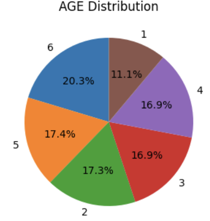
Figure 1: Slightly imbalanced age groups (primary dataset).

Buckets and their corresponding age ranges:
1) 18-24, 2) 25-34, 3) 35-44, 4) 45-54, 5) 55-64, and 6) 65+.

States were overall evenly represented in both datasets (not accounting for different relative sizes of state populations), although California ($5$) and Oregon ($38$) had higher relative representation (Figure 2).

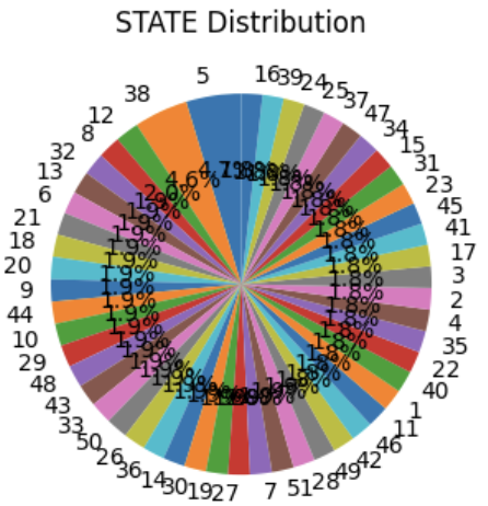
Figure 2: CA and OR with increased state representation (primary dataset).

Imbalance between the treatment and control group covariates in the primary dataset is visualized as shown in Figure 3 using xBalance from the RITools R package (Jake Bowers and Mark Fredrickson and Ben Hansen and Josh Errickson, 2023). We see that without any manipulation, covariates are poorly balanced between the groups.

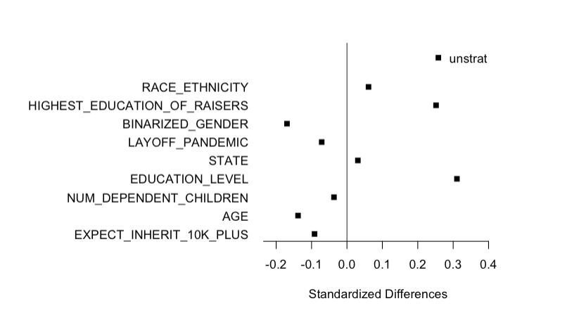
Figure 3: Covariate imbalance in primary dataset.

3.4 Feature Engineering the Outcome Variable

Towards having a single score indicating an individual’s overall financial health, we engineer a FIN_HEALTH variable by taking the sum of our financial health marker variables, after they have been standardized to have answer ranges of $0-9$ (Appendix B). For our primary analysis, this sum of financial health markers is our outcome variable. We chose not to perform further manipulation on our primary analysis to minimize potential for biases and assumptions in our analysis. Given markers $m_{1},...,m_{17}$ we calculate financial health score by:

$$\text{FIN\_HEALTH}=\text{sum}(m_{1},...,m_{1}7)$$

The resulting financial health score distribution for the primary dataset is as shown in Figure 4. The distribution of financial health scores for our secondary analysis of high-school literacy courses can be found in Appendix H.

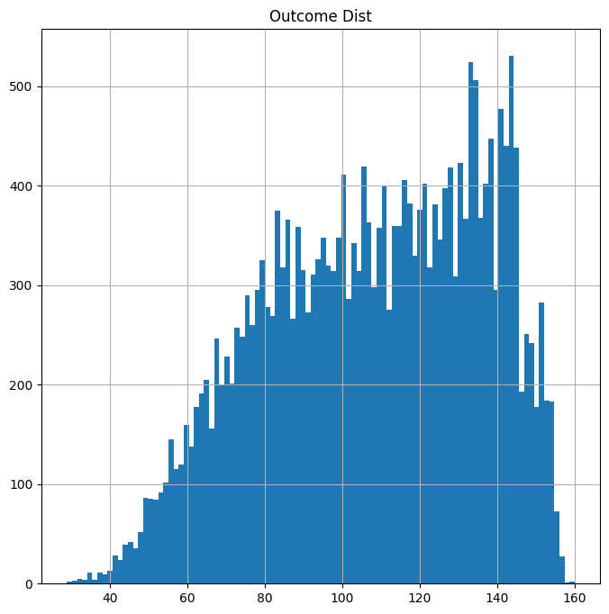
Figure 4: Distribution of financial health outcomes in primary dataset.

Though we do not add marker coefficients in the primary analysis, we do acknowledge that each of the financial health markers is not equally important. As part of our sensitivity analysis (see subsection 7.1), we scale each marker by our understanding of each marker’s relative importance in determining an individual’s financial health. Now given each marker $m_{1},...,m_{17}$ we calculate the scaled financial health score by:

$$\text{FIN\_HEALTH\_SC}=\hskip 2.84526pt m_{1}+m_{2}+m_{3}+0.5\cdot m_{4}+0.5\cdot m_{5}$$

$$+m_{6}+0.25\cdot m_{7}+0.25\cdot m_{8}$$

$$+0.5\cdot m_{9}+m_{10}$$

$$+0.75\cdot m_{11}+m_{12}$$

$$+1.25\cdot m_{13}+0.5\cdot m_{14}$$

$$+2\cdot m_{15}+m_{16}+0.5\cdot m_{17}$$

The distributions of scaled financial health score can be found in Appendix I.

3.5 Data Limitations

As all data in this study is purely observational, we conducted our experiments in the framework of observational study design. Furthermore, the data did not contain any information about the level of financial education received by study participants. As a result, our treatment variable $Z$ merely indicated whether a participant received education (treated) or not (control) and our treatment effect measured only the effect of attendance, regardless of level of engagement. As mentioned earlier, the NFCS dataset had very poor standardization of answer options, so we had to re-scale and re-order answer results for consistency. Notably, we did not consider the psychology or probability distributions for different ranges of answer options (eg. Does a $1-10$ answer range yield more moderate responses/less extreme responses compared to a $1-4$ answer range?).

4 Methods

Since we had many pre-treatment covariates that could potentially confound our outcome, we elected to use causal inference methodologies that robustly identify treatment effects when pre-treatment covariates are present. In order to do this, we made some key assumptions. For each unit $i$, we have treatment indicator $Z_{i}$, pre-treatment covariates $X_{i}$, and potential outcomes $Y_{i}(0)$ and $Y_{i}(1)$, all assumed to be iid. This assumption was necessary due to the observational nature of our data - whereas in a randomization model with good controlled study design we could make the assumption that $Z\perp\{Y(0),Y(1)\}$, in the observational setting we need to make the assumption of ignorability:

$$(Y(0),Y(1))\perp Z|X$$

This assumption means that, given identical covariates $X$, exposure to the treatment is independent of the potential outcomes $Y(0)$ and $Y(1)$. By making this assumption, methods that effectively control for covariates $X$ can isolate observed differences in the outcome $Y$ due solely to the treatment.

A quantity of interest in many of the estimators used in this section is the propensity score. The propensity score is defined as the probability of receiving the treatment, conditioned on covariates and potential outcomes:

$$e(X,Y(1),Y(0)) =p(Z=1|X,Y(0),Y(1))$$

$$=p(Z=1|X)$$

$$e(X) =p(Z=1|X)$$

where the second equality comes from the assumption of ignorability. It can be shown that:

$$Z\perp(Y(1),Y(0))|X$$

$$\implies Z\perp(Y(1),Y(0))|e(X)$$

The proof of this can be found in Appendix C. From this result, it follows that we can adjust our estimator using the single-dimensional propensity score instead of the potentially multi-dimensional covariates, and obtain equivalent results. In practice, logistic regression models are used to approximate the propensity score $\hat{e}(X)$. We follow this literature standard in our analysis.

4.1 Generalized Lin’s / Machine Learning Estimator

Generalized Lin’s estimator is one of several useful methods for identifying treatment effects in data with pre-treatment covariates. We note here that Generalized Lin’s is typically employed only in the context of experimental data — despite this, Generalized Lin’s provides a useful signal as to whether we ought to trust our estimates from AIPW, whose variance is reduced using techniques similar to Generalized Lin’s. If the covariate distribution varies widely between treated and untreated groups, the mathematical justification of Generalized Lin’s breaks down and we should thus be wary also of AIPW confidence intervals.

For generalized Lin’s estimator, we estimate our average treatment effect (ATE) by building prediction models on treated units and control units, then using these prediction models to generate a hypothetical ‘complete‘ table of science whereby we know the outcome given treatment or control for each unit in the study. That is, for outcome variable $Y$, covariates $X$, and treatment $Z$, we learn a model $\hat{\mu_{1}}(\cdot)$ which models $Y\sim X$ for the subset of data where $Z=1$. Similarly, we learn a model $\hat{\mu_{0}}(\cdot)$ which models $Y\sim X$ for the subset of data where $Z=0$. By building these prediction models, we are inherently learning the effect of our covariates on the outcome variable. When we calculate our ATE in the end, each treatment unit now has a predicted ‘hypothetical control‘ outcome value to compare against, and vice versa for control units. Thus, we are able to better calculate the effect of the treatment in isolation from the effects of covariates.

When using modern machine-learning techniques it is critical to shift our models so that they are unbiased . We adjust each $\hat{\mu_{k}}$ as follows:

$$\tilde{\mu_{k}}(X)=\hat{\mu_{k}}(X)+\frac{1}{n_{k}}\sum_{i=1}^{n}Z_{i}\left(Y_{i}-\hat{\mu_{k}}(X_{i})\right)$$

We then calculate our ATE by:

$$\hat{\tau}_{\text{pred}} =\frac{1}{n}\left(\sum_{i:Z_{i}=1}Y_{i}+\sum_{i:Z_{i}=0}\tilde{\mu_{1}}(X_{i})\right)$$

$$-\frac{1}{n}\left(\sum_{i:Z_{i}=1}\tilde{\mu_{0}}(X_{i})+\sum_{i:Z_{i}=0}Y_{i}\right)$$

Our variance estimation can then be calculated:

$$\hat{V}_{\text{pred}} =\frac{1}{n_{1}}\hat{\sigma}^{2}(1)+\frac{1}{n_{0}}\hat{\sigma}^{2}(0)+\frac{1}{n}\hat{\sigma}^{2}(\tau)$$

$$\text{where }\hat{\sigma}^{2}(1) =\frac{1}{n_{1}-1}\sum_{i:Z_{i}=1}(Y_{i}-\tilde{\mu_{1}}(X_{i}))^{2}$$

$$\text{and }\hat{\sigma}^{2}(0) =\frac{1}{n_{0}-1}\sum_{i:Z_{i}=0}(Y_{i}-\tilde{\mu_{0}}(X_{i}))^{2}$$

$$\text{and }\hat{\sigma}^{2}(\tau) =\frac{1}{n-1}\sum_{i=1}^{n}(\tilde{\mu}_{1}(X_{i})-\tilde{\mu}_{0}(X_{i})-\overline{\tilde{\mu}}_{1}+\overline{\tilde{\mu}}_{0})^{2}$$

$$\text{where }\overline{\tilde{\mu}}_{1} =\frac{1}{n}\sum_{j=1}^{n}\tilde{\mu}_{1}(X_{j})\text{ and }\overline{\tilde{\mu}}_{0}=\frac{1}{n}\sum_{j=1}^{n}\tilde{\mu}_{0}(X_{j})$$

Notably, in actual implementation, we perform cross-fitting to ensure that we do not overfit our models and that we get valid variance estimates. To perform cross-fitting, we split our data into two halves $I_{1}$ and $I_{2}$. We train a treated and control model for each half, then shift these models using the opposite half’s data (to make them unbiased). With the unbiased models we calculate $\hat{\tau}_{\text{pred}^{I_{1}}}$ and $\hat{\tau}_{\text{pred}^{I_{2}}}$ for each half. Finally, we take the weighted average of these two estimators (weighting by relative size of each half in case of an imperfect split), to calculate our overall $\hat{\tau}_{\text{pred}}$. The full algorithm for cross-fitting with Generalized Lin’s Estimator can be found in Appendix E.

For this analysis, we implemented cross-fitting in R with random forest as our model framework for training each $\hat{\mu_{k}}(\cdot)$ (models trained using the randomForest R package (Liaw & Wiener, 2022)).

4.2 Propensity Matching

Propensity matching is a matched pairs design technique for estimating the average treatment effect by comparing treated units with control units that have similar or identical covariates $X$. In this analysis, we used 1:1 matching, where control units were matched with at most one treated unit. In general, it is difficult to find exact matching for each control unit, and so approximate matching tecniques are used. In approximate matching, treatment units $i$ are matched with control units $m(i)$ where:

$$m(i)=\arg\min_{k:Z_{k}=0}d(X_{i},X_{k})$$

where $d$ is some distance metric in the covariate space. Commonly used is the Mahalanobis distance, defined as:

$$d(X_{i},X_{k})=(X_{i}-X_{k})^{T}\hat{\Sigma}^{-1}(X_{i}-X_{k})$$

where $\hat{\Sigma}^{-1}$ is the sample covariance matrix of $X$. Similar is the robust Mahalanobis distance, which follows the same equation, but where $X$ is replaced by $\text{rank}(X)$. In order to ensure units are close in propensity score, caliper matching further enforces the condition that:

$$|\hat{e}(X_{i})-\hat{e}(X_{k})|\leq c\cdot sd(\hat{e}(X))$$

It is important to note that even after caliper matching, there may still be covariate imbalances between treatment and control groups — however, with effective matching, this is minimized, reducing the impact of confounders on biases on the treatment effect estimate. In 1:1 matching, we can first calculate an initial estimate for the treatment effect, and then adjust for any biases. The initial estimate is given by:

$$\hat{\tau}^{m}=\frac{1}{n_{1}}\sum_{i:Z_{i}=1}(Y_{i}(1)-Y_{m(i)}(0))$$

where $n_{1}$ is the number of treated units, and $Y_{m(i)}(0)$ is the observed outcome of the control unit matched with treatment unit $i$. The bias in this term can be corrected for using the following (Abadie & Imbens, 2011):

$$\hat{B}=\frac{1}{n_{1}}\sum_{i:Z_{i}=1}\hat{B}_{i}$$

$$\hat{B}_{i}=\hat{\mu}_{0}(X_{i})-\hat{\mu}_{0}(X_{m(i)})$$

where $\hat{\mu}_{0}$ is an estimate of $E[Y|Z=0,X=X]$ which can be fit using linear regression methods. The bias adjusted estimator is then given by:

$$\hat{\tau}^{caliper}=\hat{\tau}^{m}-\hat{B}$$

In this analysis, we use the DOS2, optmatch, and rcbalance packages in R to perform 1:1 matching using robust Mahalanobis distance, with different caliper values of 0.1, 0.2, and 0.05, before using these matched pairs to compute a bias-corrected estimate of the average treatment effect (Rosenbaum, 2007; Hansen & Bowers, 2022; Baum, 2021).

4.3 IPW

Inverse propensity score weighting (IPW) is the basis for two estimators of the treatment effect used in the present analysis — the Horvitz-Thompson estimator (Horvitz & Thompson, 1952), and the Hajek estimator. Both estimators rely on the following result, which holds under ignorability. The proof is shown in Appendix D:

$$E[Y(1)] =E\left[\frac{ZY}{e(X)}\right]$$

$$E[Y(0)] =E\left[\frac{(1-Z)Y}{1-e(X)}\right]$$

This result motivates an estimator:

$$\hat{\tau}^{ht}=\frac{1}{n}\sum_{i=1}^{n}\frac{Z_{i}Y_{i}}{\hat{e}(X_{i})}-\frac{(1-Z_{i})Y_{i}}{(1-\hat{e}(X_{i}))}$$

Essentially, this estimator is constructed by weighting the observation of each individual in the sample by their propensity score. Since $e(x)$ is bounded to be between 0 and 1, this estimator can often experience instability for observations that have high or low propensity scores - to remedy this issue, truncation is sometimes used, where propensity scores are limited as follows:

$$\hat{e}(X)\leftarrow\min(0.975,\max(\hat{e}(X),0.025))$$

An additional shortcoming of this estimator is that it is not invariant under transformations of the outcome variable. To show this, let $\tilde{Y}=Y+c$:

$$\hat{\tau}^{ht}(Y)-\hat{\tau}^{ht}(\tilde{Y}) =\frac{1}{n}\sum_{i=1}^{n}\frac{Z_{i}Y_{i}}{\hat{e}(X_{i})}-\frac{(1-Z_{i})Y_{i}}{(1-\hat{e}(X_{i}))}$$

$$-\frac{1}{n}\sum_{i=1}^{n}\frac{Z_{i}(Y_{i}+c)}{\hat{e}(X_{i})}-\frac{(1-Z_{i})(Y_{i}+c)}{(1-\hat{e}(X_{i}))}$$

If we rearrange terms to have a common denominator and factor them out, this can equivalently be written as:

$$\frac{1}{n}\sum_{i=1}^{n}\frac{1}{\hat{e}(X_{i})(1-\hat{e}(X_{i}))} \bigg{(}Z_{i}Y_{i}-Z_{i}Y_{i}\hat{e}(X_{i})-Y_{i}\hat{e}(X_{i})$$

$$+Z_{i}Y_{i}\hat{e}(X_{i})Z_{i}Y_{i}+Z_{i}Y_{i}\hat{e}(X_{i})$$

$$-Z_{i}c+Z_{i}c\hat{e}(X_{i})+Y_{i}\hat{e}(X_{i})+$$

$$c\hat{e}(X_{i})-Z_{i}Y_{i}\hat{e}(X_{i})-Z_{i}c\hat{e}(X_{i})\bigg{)}$$

When canceling terms, we are left with:

$$\frac{1}{n}\sum_{i=1}^{n}\frac{c(\hat{e}(X_{i})-Z_{i})}{\hat{e}(X_{i})(1-\hat{e}(X_{i}))}\neq 0$$

concluding the proof. In this analysis, we have constructed our outcome variable as a composition of several variables, and so this property is undesirable. This motivates the location-invariant Hajek estimator:

$$\hat{\tau}^{hajek}=\frac{\sum_{i=1}^{n}\frac{Z_{i}Y_{i}}{\hat{e}(X_{i})}}{\sum_{i=1}^{n}\frac{Z_{i}}{\hat{e}(X_{i})}}-\frac{\sum_{i=1}^{n}\frac{(1-Z_{i}Y_{i}}{(1-\hat{e}(X_{i}))}}{\sum_{i=1}^{n}\frac{(1-Z_{i})}{(1-\hat{e}(X_{i}))}}$$

For the implementation of both of these methods, the propensity score model $\hat{e}(X_{i})$ was fit using logistic regression. The Hajek estimator was calculated using the PSweight package (Zhou et al., 2022), and the Horvitz-Thompson estimator was implemented directly using base R functions.

4.4 AIPW

A potential issue with using IPW based estimators is that they have high variance. This motivates the Augmented Inverse Propensity Score Weighted estimator (AIPW), which applies the idea of inverse propensity weighting to a general function $g$ of the covariates $X$. Directly applying such a function in the IPW introduces bias into the estimator, but this bias term can be computationally corrected for, resulting in an overall unbiased estimator. To show this, we can observe that for any function $g(X)$, the following is true:

$$E\left[\frac{1}{n}\sum_{i=1}^{n}\frac{Z_{i}g(X_{i})}{e(X_{i})}-\frac{1}{n}\sum_{i=1}^{n}g(X_{i})\right]$$

$$=\frac{1}{n}\sum_{i=1}^{n}\bigg{(}E\bigg{[}\frac{Z_{i}g(X_{i})}{e(X_{i})}\bigg{]}-E[g(X_{i})]\bigg{)}$$

$$=\frac{1}{n}\sum_{i=1}^{n}\bigg{(}E\bigg{[}\frac{E[Z_{i}|X_{i}]g(X_{i})}{e(X_{i})}\bigg{]}-E[g(X_{i})]\bigg{)}$$

$$=\frac{1}{n}\sum_{i=1}^{n}\bigg{(}E\bigg{[}\frac{e(X_{i})g(X_{i})}{e(X_{i})}\bigg{]}-E[g(X_{i})]\bigg{)}$$

$$=\frac{1}{n}\sum_{i=1}^{n}(E[g(X_{i})]-E[g(X_{i})])=0$$

Similarly, it can be shown that:

$$E\left[\frac{1}{n}\sum_{i=1}^{n}\frac{(1-Z_{i})g(X_{i})}{(1-e(X_{i}))}-\frac{1}{n}\sum_{i=1}^{n}g(X_{i})\right]=0$$

We can therefore form a reduced estimator by first fitting a logistic regression model to estimate $\hat{e}(X)$, fitting linear models $\hat{\mu}_{1}(X)$ and $\hat{\mu}_{0}(X)$ that fit:

$$\mu_{1}(X)=E[Y|Z=1,X=x]$$

$$\mu_{0}(X)=E[Y|Z=0,X=x]$$

and fitting adjusted linear models:

$$\hat{\mu}_{1}^{adj} =\frac{1}{n}\sum_{i=1}^{n}\frac{Z_{i}(Y_{i}-\hat{\mu}_{1}(X_{i}))}{\hat{e}(X_{i})}+\hat{\mu}_{1}(X_{i})$$

$$\hat{\mu}_{0}^{adj} =\frac{1}{n}\sum_{i=1}^{n}\frac{(1-Z_{i})(Y_{i}-\hat{\mu}_{0}(X_{i}))}{(1-\hat{e}(X_{i}))}+\hat{\mu}_{0}(X_{i})$$

From this, we form the following AIPW estimator:

$$\hat{\tau}^{aipw}=\hat{\mu}_{1}^{adj}-\hat{\mu}_{1}^{adj}$$

In this analysis, this estimator was calculated using the AIPW package (Yongqi Zhong et al., 2021), which forms confidence intervals using cross-fitting to estimate the variance. This estimator is known as the ‘doubly-robust’ estimator, because it only requires either the outcome models $\hat{\mu}^{adj}$ or the propensity scores $e(X)$ to be accurate in expectation in order for the treatment effect estimate to be correct (Bang & Robins, 2005). Thus, AIPW incorporates robustness benefits from both Generalized Lin’s Estimator and IPW.

5 Primary Experiments and Results

Estimates of the average treatment effect of financial education on financial health score for all estimation techniques are shown in Table 1. Also included are variance estimates and $95$% confidence intervals for the treatment effect.

Table 1: ATEs for primary analysis.

Estimator	ATE	$\hat{V}$	95% CI
Generalized Lin’s	3.99	0.13	3.27 - 4.70
Horvitz-Thompson	3.71	0.35	3.02 - 4.40
Hajek	3.71	0.25	3.31 - 4.18
AIPW	3.55	0.382	2.80 - 4.30
Matching (caliper=0.1)	2.91	0.20	2.04 - 3.78
Matching (caliper=0.2)	2.75	0.20	1.88 - 3.61
Matching (caliper=0.05)	3.13	0.20	2.26 - 4.00

6 Secondary Experiments and Results: HS Financial Literacy Courses

Estimates of the average treatment effect of high-school based financial literacy education on financial health score for all estimation techniques are shown in Table 2. Also included are variance estimates and $95$% confidence intervals for the treatment effect.

Table 2: ATEs for unscaled secondary analysis.

Estimator	ATE	$\hat{V}$	95% CI
Generalized Lin’s	1.53	0.43	0.24 - 2.81
Horvitz-Thompson	2.28	0.72	0.87 - 3.69
Hajek	2.28	0.76	0.79 - 3.46
AIPW	1.85	0.69	0.51 - 3.19
Matching (caliper=0.1)	1.48	0.49	0.10 - 2.85
Matching (caliper=0.05)	1.44	0.49	0.06 - 2.81
Matching (caliper=0.2)	1.58	0.49	0.21 - 2.96

7 Sensitivity Analysis

7.1 Modified Financial Health Score Function

In order to confirm the robustness of our results, the average treatment effects were also estimated for FIN_HEALTH_SC outcomes with different weights applied to each financial health marker, as described at the end of subsection 3.4. These average treatment effects, and their corresponding variance estimates and confidence intervals can be found in Table 3 and Table 4.

7.1.1 Primary Analysis

Table 3: ATEs for scaled primary analysis.

Estimator	ATE	$\hat{V}$	95% CI
Generalized Lin’s	2.70	0.10	2.09 - 3.31
Horvitz-Thompson	2.59	0.29	2.02 - 3.17
Hajek	2.59	0.33	1.84 - 3.12
AIPW	2.47	0.32	1.83 - 3.10
Matching (caliper=0.1)	2.03	0.14	1.29 - 2.78
Matching (caliper=0.2)	1.91	0.14	1.17 - 2.66
Matching (caliper=0.05)	2.21	0.14	1.47 - 2.95

7.1.2 Secondary Analysis

See Table 4 for the weighted financial health score function results on the HS financial education analysis.

Table 4: ATEs for scaled secondary analysis.

Estimator	ATE	$\hat{V}$	95% CI
Generalized Lin’s	1.34	0.32	0.24 - 2.44
Horvitz-Thompson	1.82	0.60	0.63 - 3.00
Hajek	1.82	0.55	0.90 - 3.07
AIPW	1.46	0.58	0.32 - 2.61
Matching (caliper=0.1)	1.11	0.36	-0.08 - 2.29
Matching (caliper=0.05)	1.06	0.36	-0.12 - 2.24
Matching (caliper=0.2)	1.19	0.36	0.01 - 2.37

7.2 Testing Different Calipers

We conducted further sensitivity analysis by repeating the 1:1 matched pairs design with several different calipers. While a 0.1 caliper is commonly used, and seemed the most apt for our estimation due to its relatively strong resultant covariate balance and average difference between propensity scores in each pair, we also estimated our ATE with calipers of 0.05 and 0.2 to test for robustness. We observed estimates for the ATE and Variance that were very similar across each caliper.

8 Discussion

8.1 Effect of Financial Literacy Education on Financial Health

All estimation methods in Table 1 provide strong statistical evidence to indicate that financial education positively impacts financial health. All of these results were significant at the 5% confidence level. As expected, the inverse propensity-weighted estimators had the highest variance, but still provided sufficient evidence to reject the null hypothesis that financial education has no impact on financial health.

Notably, however, the magnitude of the effect was quite small, ranging from $1.17-3.31$ points from minimum to max across all methods. Relative to the scale of the financial health score used here (average score was $112$ for treated units, and $115$ for controls), our results indicate an isolated treatment effect of approximately 3% improvement due to receiving financial literacy education.

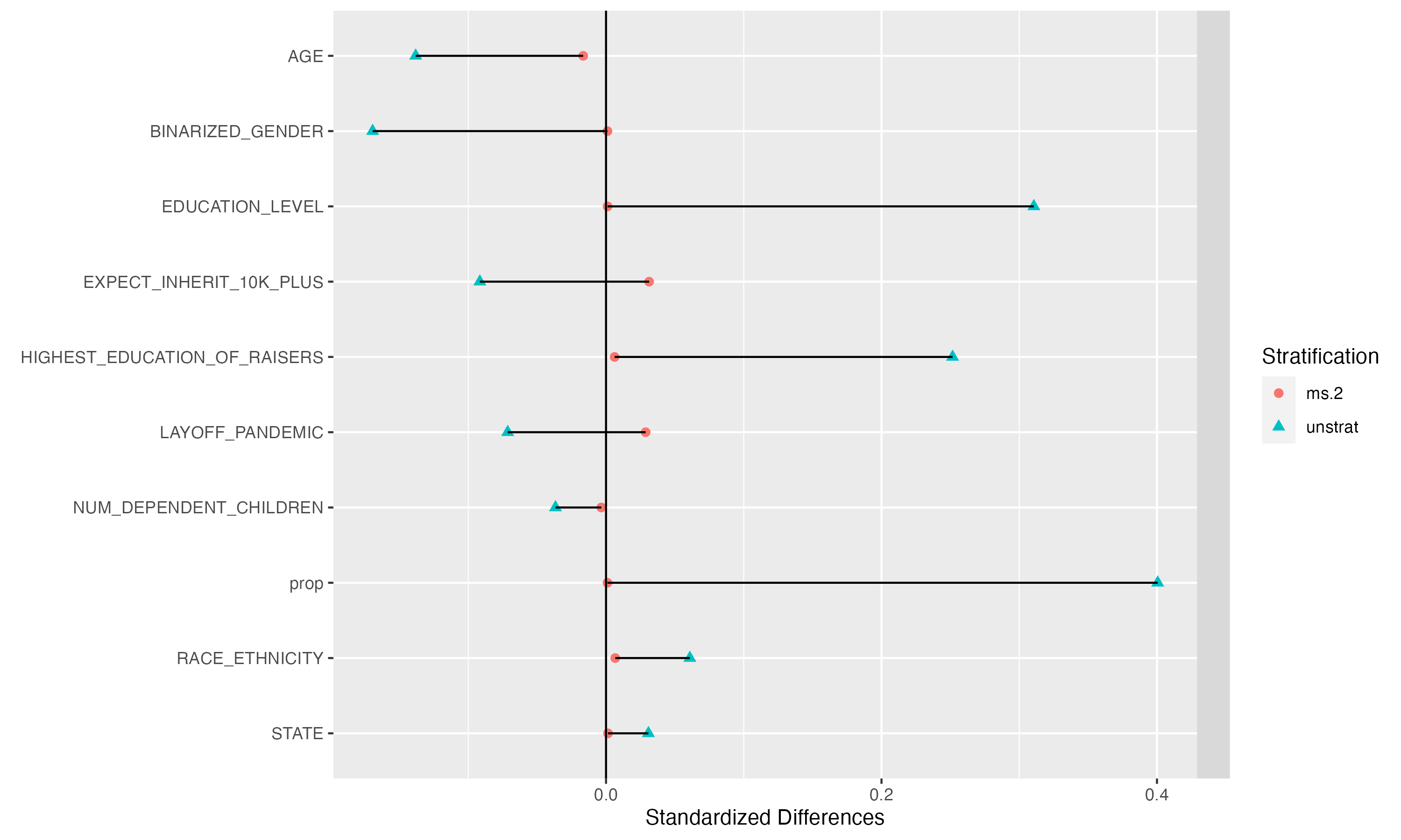
Figure 7: Covariate imbalance before and after matched pairs stratification in primary dataset.

Propensity matching was highly effective at reducing covariate imbalance between matched pairs in the setting of the primary treatment variable. As seen in Appendix Figure 7, standardized differences within the unstratified data were relatively high, most notably for highest_education_of_raisers, education_level and our propensity scores, at $0.25$, $0.31$, and $0.4$, respectively. But within the matched pairs, each difference dropped to $<0.025$.

8.2 Effect of High-School Literacy Education on Financial Health

We observe a weaker average treatment effect when specifically investigating the effects of financial education received in high-school on financial health score (Table 2). Although weaker, the results do again provide statistical evidence to reject the null at the 5% confidence level. Notably, the control group for this secondary analysis includes individuals who may have received financial education elsewhere from high-school, weakening our power to identify an effect.

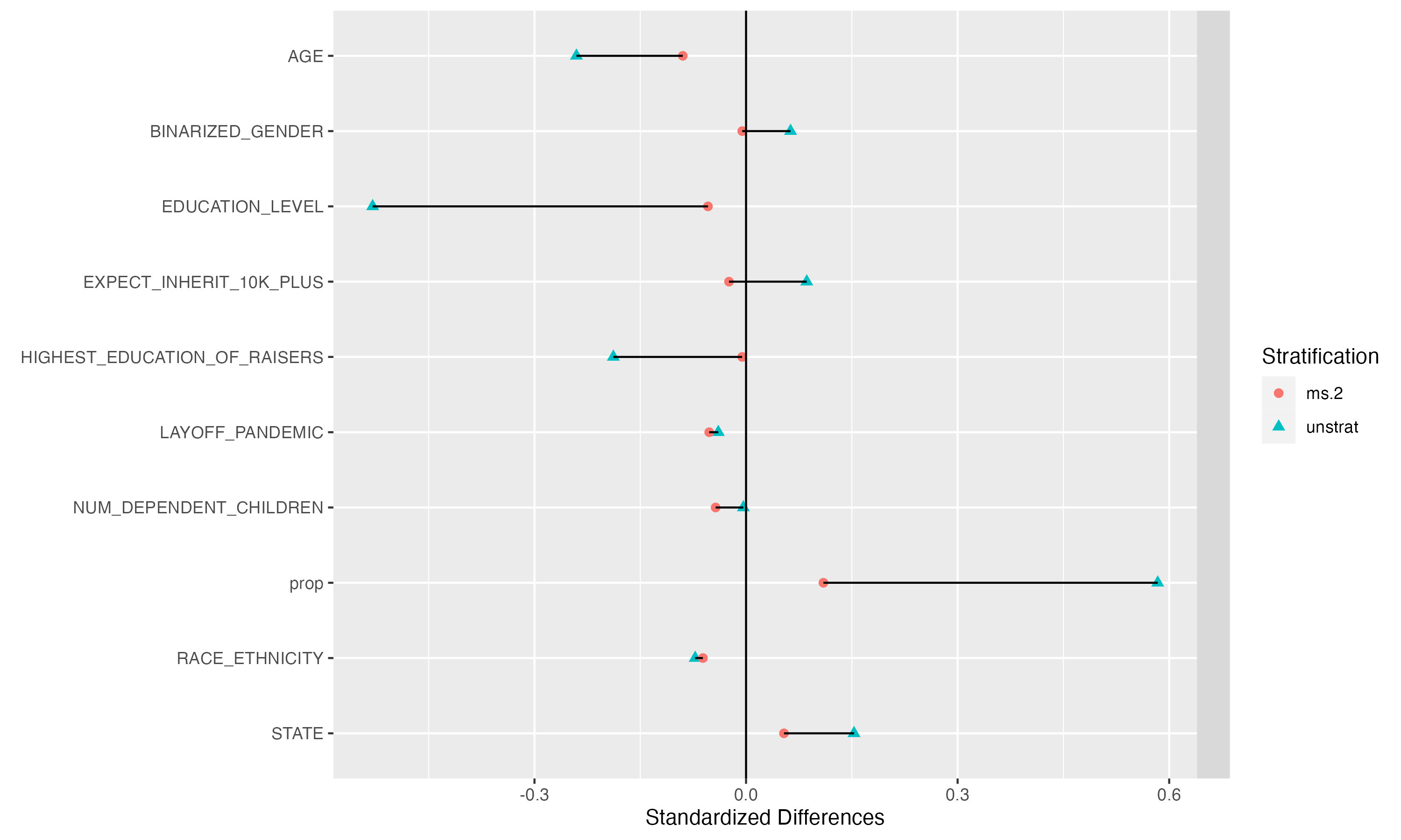
Figure 8: Covariate imbalance before and after matched pairs stratification in HS literacy dataset.

Propensity matching effectively reduced covariate imbalance between matched pairs in our secondary experiment as well, albeit not to the same degree as the primary analysis. This may be due to a smaller pool of controls for selecting optimal matches Appendix G. As we show in Appendix Figure 8, standardized differences within the unstratified data were relatively high, most notably with education_level exceeding 0.4, and our propensity scores approaching 0.6. After matching, differences dramatically improve, with a maximum distance of around $0.25$.

8.3 Sensitivity Analysis

For the primary analysis, average treatment effect estimates using our weighted financial health score outcome function were broadly similar to those in the original analysis (Table 3). Both the direction and the significance of the results remained consistent with the original analysis, providing evidence that our analysis is robust to variations in the exact computation of the financial health outcome.

When focusing on HS-based financial education, the average treatment effect estimates using the weighted financial health score were not all significant at the 5% level (Table 4). In particular, caliper matching with caliper sizes of $0.1$ and $0.05$ yielded $95$% confidence intervals containing $0$. This is an indicator that the matched pairs estimator was not robust to scaling in the outcome variable. However, all other estimators still indicated a positive treatment effect at the 5% significance level, indicating that on the whole, there is evidence that HS-based financial education has a positive effect on financial health, even when manipulating the exact financial health measurement function.

8.4 Limitations

While the NFCS data was sprawling in both number of respondents and number of topics covered, it had some limitations for our question of interest. The data did not describe how long ago survey respondents received financial literacy education, making it harder to filter the data and isolate the effect for people who have recently received the treatment, but with enough time for its potential benefits to be realized. Many variables were binned into groupings that limited the amount of information available to researchers. Perhaps most importantly, many responses we used in calculating financial health outcome scores were self-assessments of the individual’s financial health, and these standards may vary from person to person.

9 Conclusion

This study used data from the 2021 NFCS to understand the causal effect of financial education on aggregated financial health outcomes. Our results provide strong statistical evidence that financial education positively impacts financial health scores, though the magnitude of that effect is potentially quite weak. These results were robust to numerous causal effect estimation techniques, as well as sensitivity analysis on matching caliper choices and differently constructed composite financial health scores. Our results may prove useful to policymakers considering implementing financial education requirements in public school systems. Moreover, these findings suggest that any individual considering financial education is highly likely to benefit from such an education.

Future works should focus on devising a more informed formulation for the financial health score, based on domain expertise. None of the authors of this work are primarily involved in the study of finance, education, or long term financial health trajectories. An extension of the current research complemented by domain-expert insight in the outcome variable would likely yield much more interpretable results for estimating the real-world benefit of the ATE.

10 Contributions

Arnav and Charles performed initial literature review. All contributors collaborated in determining experimental process, and defining covariates, treatment variables, and outcomes. Daniel wrote the data processing code and Generalized Lin’s Estimator experiment code. Charles wrote the propensity matching experiment code. Arnav wrote the IPW and AIPW experiment code. All contributors contributed in writing the final paper.

11 Code

All code for this work can be found at https://github.com/danielfrees/finlitCausal.

Appendix A Covariate List

Table 5: List of Covariates

Covariates

1. RACE_ETHNICITY 2. EDUCATION_LEVEL 3. HIGHEST_EDUCATION_OF_RAISERS 4. NUM_DEPENDENT_CHILDREN 5. BINARIZED_GENDER 6. AGE 7. LAYOFF_PANDEMIC 8. EXPECT_INHERIT_10K_PLUS 9. STATE

Appendix B Financial Health Markers

Table 6: List of Financial Health Markers

Financial Health Markers

1. ’SATISFACTION_WITH_FINANCIAL_CONDITION’ 2. ’SPENDING_COMPARISON_TO_INCOME’ 3. ’DIFFICULTY_COVERING_EXPENSES’ 4. ’EMERGENCY_FUNDS’ 5. ’CONFIDENCE_GET_2000’ 6. ’CREDIT_RECORD_RATING’ 7. ’CHECKING_ACCOUNT’ 8. ’SAVINGS_ACCOUNT’ 9. ’OVERDRAW_CHECKING_ACCOUNT’ 10. ’REGULAR_CONTRIBUTION_TO_RETIREMENT’ 11. ’OTHER_INVESTMENTS’ 12. ’ALWAYS_PAY_CR_FULL_12MO’ 13. ’USED_PAYDAY_LOAN’ 14. ’DEBT_COLLECTED_12MO’ 15. ’TOO_MUCH_DEBT_STRENGTH’ 16. ’D2D_FINANCIAL_SKILL’ 17. ’FINANCIAL_KNOWLEDGE_ASSESS’

Appendix C Conditional Independence based on Propensity

Our goal is to show:

$$Z\perp(Y(1),Y(0))|X\implies Z\perp(Y(1),Y(0))|e(X)$$

Equivalently, we can show:

$$P(Z=1|Y(1),Y(0),e(X)) =p(Z=1|e(X))$$

For the top term, we can argue:

$$P(Z=1|Y(1),Y(0),e(X)) =E[Z|Y(1),Y(0),e(x)]$$

$$=E[E[Z|Y(1),Y(0),X]|Y(1,Y(0),e(X)]$$

$$=E[e(X)|Y(1),Y(0),e(X)]$$

$$=e(X)$$

Similarly, for the bottom term:

$$P(Z=1|e(X))=E[Z|e(X)] =E[E[Z|X]|e(X)]$$

$$=E[e(X)|e(X)]$$

$$=e(X)$$

Appendix D Propensity estimator is equal in expectation to treatment effect

We will show the proof for:

$$E[Y(1)]=E\left[\frac{ZY}{e(X)}\right]$$

as the proof for the other expression is analogous:

$$E\left[\frac{ZY}{e(X)}\right] =E[E\left[\frac{ZY}{e(X)}|X\right]]$$

$$=E[\frac{1}{e(X)}E[ZY(1)|X]]$$

$$=E[\frac{1}{e(X)}E[Z|X]E[Y(1)|X]]$$

$$=E[\frac{1}{e(X)}e(X)E[Y(1)|X]]$$

$$=E[E[Y(1)|X]]$$

$$=E[Y(1)]$$

where the move from $Y$ to $Y(1)$ comes from the consistency of the outcome depending on the treatment, and the third equality comes from the conditional independence of $Z$ and $Y(1)$.

Appendix E Cross-fitting Algorithm for Generalized Lin’s / Machine Learning Estimator

Here we describe the algorithm for calculating the Generalized Lin’s / Machine Learning average treatment effect estimate and variance estimate via cross-fitting on outcome $Y$, covariates $X=X_{1},...X_{n}$, and treatment $Z\in{0,1}$ using randomForest as the model. Note that we denote two halves of the data used for cross-fitting as $I_{1},I_{2}$, and in half $k$ we denote the treated examples as $I_{k}^{+}$ and controls as $I_{1}^{-}$.

Algorithm 1 ML Estimator Crossfitting ATE and Variance Estimation

  Input: data $D$, size $n$

  $I_{1},I_{2}\leftarrow$ random split of $D$ into halves.

  for $k\in{1,2}$ do

     $\hat{\mu_{1}}^{k}(X)\leftarrow\text{randomForest}(Y\sim X_{1}+...+X_{n},\text{data}=I_{k},\text{subset }Z=1)$

     $\hat{\mu_{0}}^{k}(X)\leftarrow\text{randomForest}(Y\sim X_{1}+...+X_{n},\text{data}=I_{k},\text{subset }Z=0)$

     $\tilde{\mu_{1}}^{k}(\cdot)=\hat{\mu_{1}}^{k}(\cdot)+\frac{1}{|I_{(1-k)}^{+}|}\sum_{i\in I_{(1-k)}}Z^{(i)}(Y^{(i)}-\hat{\mu_{1}}^{k}(X^{(i)}))$

     $\tilde{\mu_{0}}^{k}(\cdot)=\hat{\mu_{0}}^{k}(\cdot)+\frac{1}{|I_{(1-k)}^{-}|}\sum_{i\in I_{(1-k)}}(1-Z^{(i)})(Y^{(i)}-\hat{\mu_{0}}^{k}(X^{(i)}))$

     $\hat{\tau}^{I_{k}}\leftarrow\frac{1}{|I_{k}|}\left(\sum_{i\in I_{k}}Z_{i}Y_{i}+(1-Z_{i})\tilde{\mu_{1}}^{(1-k)}(X_{i})-\sum_{i\in I_{k}}(1-Z_{i})Y_{i}+Z_{i}\tilde{\mu_{0}}^{(1-k)}(X_{i})\right)$

  end for

  $\hat{\tau}^{\text{pred}}\leftarrow\frac{|I_{1}|}{n}\hat{\tau}^{I_{1}}+\frac{|I_{2}|}{n}\hat{\tau}^{I_{2}}$

  for $k\in{1,2}$ do

     $\hat{\sigma}^{2}_{I_{k}}(1)\leftarrow\frac{1}{|I_{k}^{+}|-1}\sum_{i\in I_{k}}Z_{i}(Y_{i}-\tilde{\mu}_{1}^{I_{(1-k)}}(X_{i}))^{2}$

     $\hat{\sigma}^{2}_{I_{k}}(0)\leftarrow\frac{1}{|I_{k}^{-}|-1}\sum_{i\in I_{k}}(1-Z_{i})(Y_{i}-\tilde{\mu}_{0}^{I_{(1-k)}}(X_{i}))^{2}$

     $\bar{\tilde{\mu}}_{1}^{I_{(1-k)}}\leftarrow\frac{1}{|I_{k}|}\tilde{\mu}_{1}^{I_{(1-k)}}(X_{i})$

     $\bar{\tilde{\mu}}_{0}^{I_{(1-k)}}\leftarrow\frac{1}{|I_{k}|}\tilde{\mu}_{0}^{I_{(1-k)}}(X_{i})$

     $\hat{\sigma}^{2}_{I_{k}}(\tau)\leftarrow\frac{1}{|I_{k}|-1}\sum_{i\in I_{k}}\left(\tilde{\mu}_{1}^{I_{(1-k)}}(X_{i}))-\tilde{\mu}_{0}^{I_{(1-k)}}(X_{i})-\left(\bar{\tilde{\mu}}_{1}^{I_{(1-k)}}-\bar{\tilde{\mu}}_{0}^{I_{(1-k)}}\right)\right)^{2}$

     $\hat{V}^{I_{k}}\leftarrow\frac{1}{|I_{k}+|}\hat{\sigma}^{2}_{I_{k}}(1)+\frac{1}{|I_{k}-|}\hat{\sigma}^{2}_{I_{k}}(0)+\frac{1}{|I_{k}|}\hat{\sigma}^{2}_{I_{k}}(\tau))$

  end for

  $\hat{V}\leftarrow\left(\frac{|I_{1}|}{n}\right)^{2}\hat{V}^{I_{1}}+\left(\frac{|I_{2}|}{n}\right)^{2}\hat{V}^{I_{2}}$

  return $\hat{\tau}^{\text{pred}},\hat{V}$

Appendix F Complete Covariate Distributions

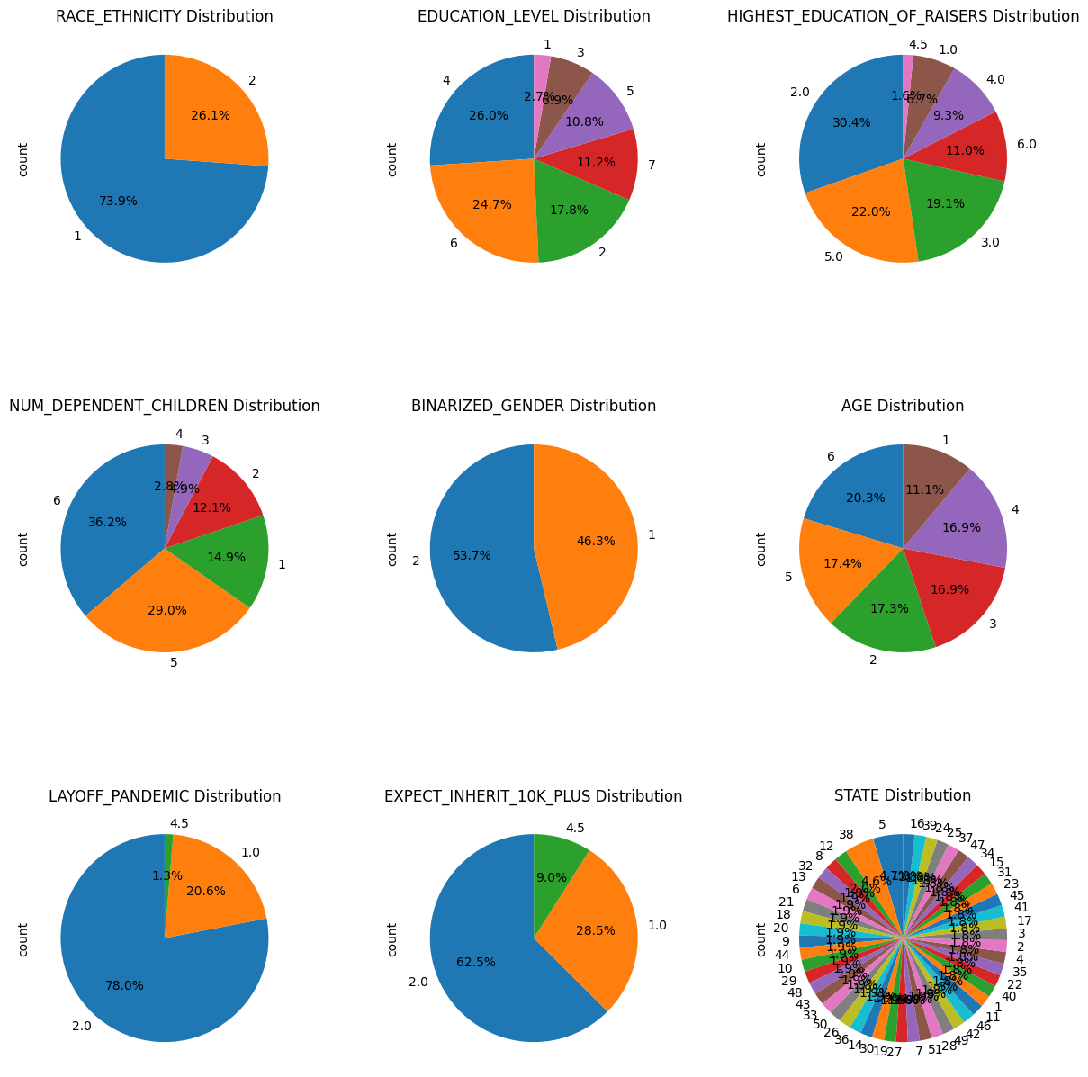
Figure 5: Distribution of covariates in primary dataset.

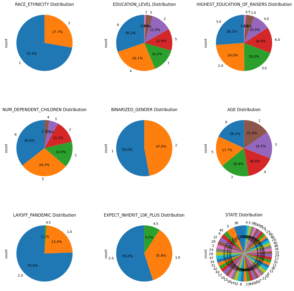
Figure 6: Distribution of covariates in HS literacy dataset.

Appendix G Treatment and Control Distributions

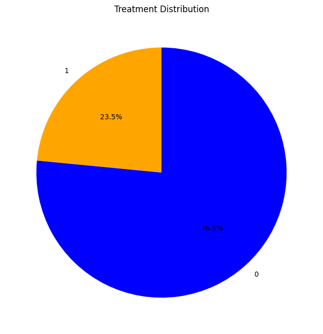
Figure 9: Distribution of treatment in primary dataset.

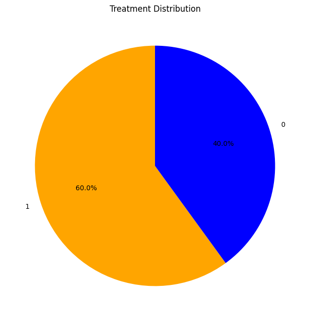
Figure 10: Distribution of treatment in HS literacy dataset.

Appendix H Secondary Analysis Financial Health Distribution

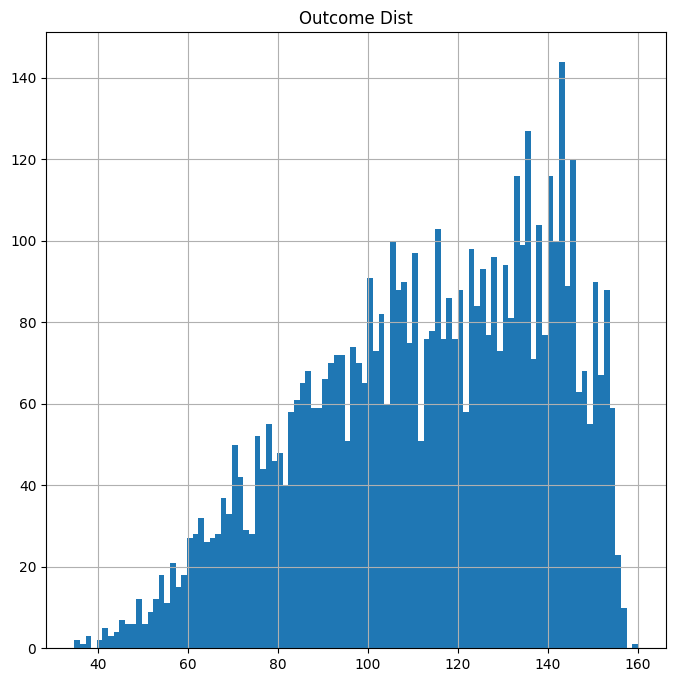
Figure 11: Distribution of financial health outcome in HS literacy dataset.

Appendix I Scaled Financial Health Distributions

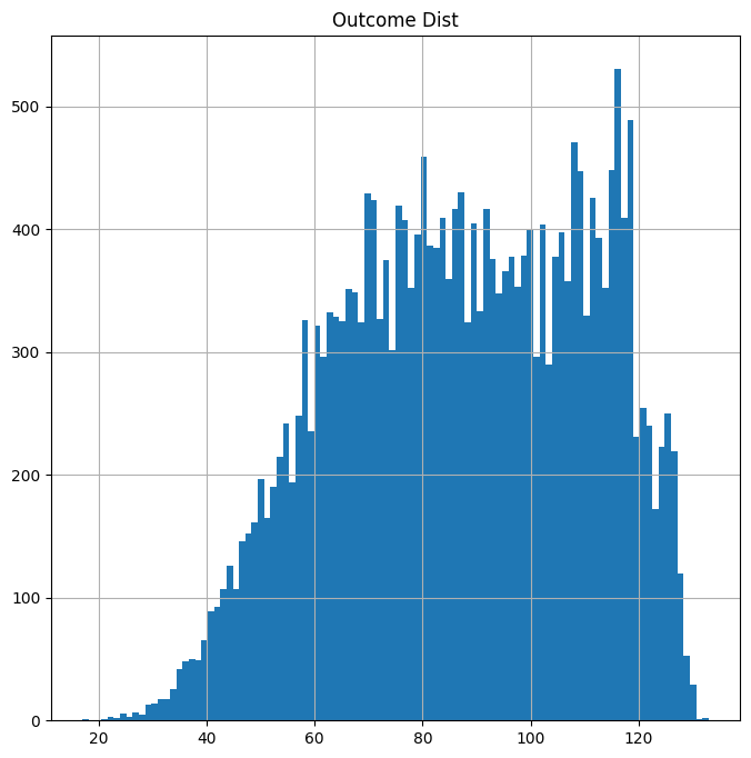
Figure 12: Distribution of scaled financial health outcome in primary dataset.

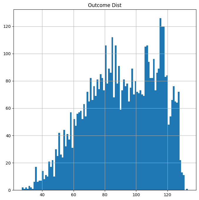
Figure 13: Distribution of scaled financial health outcome in HS literacy dataset.

References

- Abadie & Imbens (2011) Abadie, A. and Imbens, G. W. Bias-corrected matching estimators for average treatment effects. Journal of Business & Economic Statistics, 29(1):1–11, 2011.
- Bang & Robins (2005) Bang, H. and Robins, J. M. Doubly robust estimation in missing data and causal inference models. Biometrics, 61(4):962–973, 2005.
- Baum (2021) Baum, C. F. rcbalance: Large, Medium and Small Sample Balancing Weights for Covariate Balance, 2021. URL https://cran.r-project.org/package=rcbalance. R package version 0.2.2.
- Board of Governors of the Federal Reserve System (2023a) (US) Board of Governors of the Federal Reserve System (US). Consumer loans: Credit cards and other revolving plans, all commercial banks, 2023a. URL https://fred.stlouisfed.org/series/CCLACBW027SBOG. Retrieved from FRED, Federal Reserve Bank of St. Louis: November 2023.
- Board of Governors of the Federal Reserve System (2023b) (US) Board of Governors of the Federal Reserve System (US). All sectors; total mortgages; asset, level, 2023b. URL https://fred.stlouisfed.org/series/ASTMA. Retrieved from FRED, Federal Reserve Bank of St. Louis: December 2023.
- Board of Governors of the Federal Reserve System (2023c) (US) Board of Governors of the Federal Reserve System (US). Student loans owned and securitized, 2023c. URL https://fred.stlouisfed.org/series/SLOAS. Retrieved from FRED, Federal Reserve Bank of St. Louis: November 2023.
- Department of Financial Institutions, TN (2013) Department of Financial Institutions, TN. Financial education. https://www.tn.gov/tdfi/consumer-resources/financial-education.html, 2013. Accessed: 2023-12-12.
- Fan & Chatterjee (2019) Fan, L. and Chatterjee, S. Financial socialization, financial education, and student loan debt. Journal of Family and Economic Issues, 40(1):74–85, 2019.
- FINRA Investor Education Foundation (2023) FINRA Investor Education Foundation. National financial capability study data and downloads, 2023. URL https://finrafoundation.org/knowledge-we-gain-share/nfcs/data-and-downloads. Accessed: Dec 2023.
- Fry (2012) Fry, R. A record one-in-five households now owe student loan debt. Pew Research Center, September, 26, 2012.
- Hansen & Bowers (2022) Hansen, B. B. and Bowers, J. optmatch: Functions for Optimal Matching, 2022. URL https://cran.r-project.org/package=optmatch. R package version 0.9-17.
- Horvitz & Thompson (1952) Horvitz, D. G. and Thompson, D. J. A generalization of sampling without replacement from a finite universe. Journal of the American statistical Association, 47(260):663–685, 1952.
- Jake Bowers and Mark Fredrickson and Ben Hansen and Josh Errickson (2023) Jake Bowers and Mark Fredrickson and Ben Hansen and Josh Errickson. RITools: Randomization Inference Tools, 2023. URL https://www.rdocumentation.org/packages/RItools/versions/0.3-3. R package version 0.3-3.
- Kasman et al. (2018) Kasman, M., Heuberger, B., and Hammond, R. A. A review of large scale youth financial literacy education policies and programs. The Brookings Institution, 2018. Accessed December 2023.
- Liaw & Wiener (2022) Liaw, A. and Wiener, M. randomForest: Breiman and Cutler’s Random Forests for Classification and Regression, 2022. URL https://cran.r-project.org/package=randomForest. R package version 4.6-15.
- Lusardi & Mitchell (2023) Lusardi, A. and Mitchell, O. S. The importance of financial literacy: Opening a new field. Technical report, National Bureau of Economic Research, 2023.
- Martinchek et al. (2022) Martinchek, K., Andre, J., and Santillo, M. What can policymakers do to help young adults cope with debt? Gen, 10:42–57, 2022.
- McKinney (2011) McKinney, W. Pandas: a foundational python library for data analysis and statistics. Python for Data Analysis, 2011. URL https://pandas.pydata.org/.
- Ramsey Solutions (2023) Ramsey Solutions. Which States Require Financial Literacy for High School Students? — ramseysolutions.com. https://www.ramseysolutions.com/financial-literacy/states-require-financial-literacy-in-high-school, 2023. [Accessed 12-12-2023].
- Rosenbaum (2007) Rosenbaum, P. R. DOS2: Design of Observational Studies, Companion to the Second Edition, 2007. URL https://cran.r-project.org/package=DOS2. R package version 1.0-1.
- Stanford Institute for Economic Policy Research (2023) Stanford Institute for Economic Policy Research. Dollars and sense: The case for teaching personal finance. https://siepr.stanford.edu/news/dollars-and-sense-case-teaching-personal-finance, 2023. Accessed: 2023-12-12.
- Urban et al. (2020) Urban, C., Schmeiser, M., Collins, J. M., and Brown, A. The effects of high school personal financial education policies on financial behavior. Economics of Education Review, 78:101786, 2020.
- Washington Post Editorial Board (June 2022) Washington Post Editorial Board. Personal finance class should be required in high school, June 2022. URL https://www.washingtonpost.com/opinions/2022/06/12/personal-finance-class-should-be-required-high-school/. Accessed December 2023.
- Yongqi Zhong et al. (2021) Yongqi Zhong, Edward H. Kennedy, Lisa M. Bodnar, and Ashley I. Naimi. Aipw: An r package for augmented inverse probability weighted estimation of average causal effects. American Journal of Epidemiology, 2021. In Press.
- Zhou et al. (2022) Zhou, T., Tong, G., Li, F., Thomas, L., and Li, F. PSweight: Propensity Score Weighting for Causal Inference with Observational Studies and Randomized Trials, 2022. URL https://CRAN.R-project.org/package=PSweight. R package version 1.1.8.