Markov Chain Monte Carlo for Koopman-based Optimal Control: Technical Report
Abstract
We propose a Markov Chain Monte Carlo (MCMC) algorithm based on Gibbs sampling with parallel tempering to solve nonlinear optimal control problems. The algorithm is applicable to nonlinear systems with dynamics that can be approximately represented by a finite dimensional Koopman model, potentially with high dimension. This algorithm exploits linearity of the Koopman representation to achieve significant computational saving for large lifted states. We use a video-game to illustrate the use of the method.
I INTRODUCTION
This paper address the optimal control of nonlinear systems that have reasonably accurate finite-dimensional representations in terms of their Koopman operator [20]. While Koopman’s pioneering work is almost a century old, its use as a practical tool to model complex dynamics is much more recent and only became practical when computational tools became available for the analysis of systems with hundreds to thousands of dimensions. The use of Koopman models for control is even more recent, but has attracted significant attention in the last few years [9, 21, 28, 23, 6, 27].
The linear structure of the Koopman representation permits very efficient solutions for optimal control when the lifted dynamics are linear on the control input, as in [9, 21, 28]. However, linearity in the control severely limits the class of applicable dynamics. Bilinear representations are more widely applicable [23, 6, 27], but are also harder to control.
When the set of admissible control inputs is finite, the Koopman representation can be viewed as a switched linear system, where the optimal control selects, at each time step, one out of several admissible dynamics [7]. The optimal control of switched system it typically difficult [5, 31], but when the optimization criterion is linear in the lifted state, the dynamic programming cost-to-go is concave and piecewise linear, with a simple representation in terms of a minimum over a finite set of linear functions. This observation enabled the design of efficient algorithms that combine dynamic programming with dynamic pruning [7].
This paper exploits the structure of the Koopman representation to develop efficient Markov Chain Monte Carlo (MCMC) sampling method for optimal control. Following the pioneering work of [19, 10, 14], we draw samples from a Boltzmann distribution with energy proportional to the criterion to minimize. The original use of MCMC methods for combinatorial optimization relied on a gradual decrease in temperature, now commonly known as simulated annealing, to prevent the chain from getting trapped into states that do not minimize energy. An alternative approach relies on the use of multiple replicas of a Markov chain, each generating samples for a different temperature. The introduction of multiple replicas of a Markov chain to improve the mixing time can be traced back to [30]. The more recent form of parallel tempering (also known as Metropolis–coupled MCMC, or exchange Monte Carlo) is due to [15, 17].
Our key contribution is an MCMC algorithm that combines Gibbs sampling [14, 13] with parallel tempering to solve the switched linear optimizations that arise from the Koopman representation of nonlinear optimal control problems. This algorithm is computationally efficient due to the combination of two factors: (i) the linear structure of the cost function enables the full variable sweep need for Gibbs sampling to be performed with computation that scales linearly with the horizon length and (ii) parallel tempering can be fully parallelized across computation cores, as noted in [11]. With regard to (i), the computational complexity of evaluation Gibbs’ conditional distribution for each optimization variable is of order , where denotes the size of the lifted state. Our algorithm computes the conditional distributions for all variables in a full Gibbs’ sweep with computation still just of order . With regard to (ii), while here we only explore parallelization across CPU cores, in the last few years hardware parallelization using GPUs and FPGAs has achieved orders of magnitude increase in the number of samples generated with MCMC sampling [25, 3].
The remaining of this paper is organized as follows: Section II shows how a nonlinear control problem can be converted into a switching linear systems optimization, using the Koopman operator. Section III provides basic background on MCMC, Gibbs sampling, and parallel tempering. Our optimization algorithm is described in Section IV and its use is illustrated in Section V in the context of a video game.
II OPTIMAL CONTROL OF KOOPMAN MODELS
Given a discrete-time nonlinear system of the form
| (1) |
with the time taking values over , our goal is to solve a final-state optimal control problem of the form
| (2) |
where denotes the control sequence to be optimized, which we assume finite but potentially with a large number of elements.
For each input , , the Koopman operator for the system (1) operates on the linear space of functions from to and is defined by
Assuming there is a finite dimensional linear subspace of that is invariant for every Koopman operator in the family , there is an associated family of matrices such that
| (3) |
where and the functions form a basis for [12, 7, 16]. If in addition, the function in (2) also belongs to , there also exists a row vector such that
| (4) |
which enables re-writing the optimization criterion (2) as
| (5) |
We can thus view the original optimal control problem for the nonlinear system (1) as a switched linear control problem [7]. Note that it is always possible to make sure that (4) hold for some vector by including as one of the entries of .
It is generally not possible to find a finite-dimensional subspace that contains and is invariant for every . Instead, we typically work with a finite dimensional space for which (3)–(4) hold up to some error. However, to make this error small, we typically need to work with high-dimensional subspaces, i.e., large values of . Quantifying the impact on the error of the lifted space dimension and of the size of the dataset used to learn the Koopman dynamics is challenging, but notable progress has been reported in [16, 26]. Much work remains, e.g., in quantifying errors for systems with isolated limit sets [4, 22].
III MCMC METHODS FOR OPTIMIZATION
To solve a combinatorial minimization of the form
| (6) |
over a finite set , it is convenient to consider the following Boltzmann distribution with energies , :
| (7) |
for some constant . For consistency with statistical mechanics, we say that values of close to zero correspond to high temperatures, whereas large values correspond to low temperatures. The normalization function is called the canonical partition function.
For (high temperature), the Boltzmann distribution becomes uniform and all are equally probable. However, as we increase (lower the temperature) all probability mass is concentrated on the subset of that minimizes the energy . This can be seen by noting that the ratio of the probability between two is given by
which shows that the value with higher energy (and higher cost) will eventually never be selected.
This motivates a procedure to solve (6): draw samples from a random variable with Boltzmann distribution given by (7) with sufficiently high (temperature sufficiently low) so that all samples correspond to states with the minimum energy/cost.
The following result confirms that the probability that we can extract samples from the Boltzmann distribution with energies much larger than the minimum can be made arbitrarily small by increasing in proportion to just the logarithm of , provided that is sufficiently high (temperature is sufficiently low).
Lemma 1
The number of samples required to achieve a small probability is a function of the fraction of elements of that minimize . The result is particularly interesting in that the magnitude of and number of samples depends on the logarithm of this fraction, meaning that the size of could grow exponentially with respect to some scaling variable (like the time horizon in optimal control) and yet and would only need to grow linearly. However, the optimism arising from this bound needs to be tempered by the observation that this result assumes that the samples are independent and this is typically hard to achieve for large values of , as discussed below.
III-A Markov Chain Monte Carlo Sampling
Consider a discrete-time Markov chain on a finite set , with transition probability
Combining the probabilities of all possible realizations of in a row vector
and organizing the values of the transition probabilities as a transition matrix
with one per column and one per row, enables us to express the evolution of the as
A Markov chain is called regular if that there exists an integer such that all entries of are strictly positive. In essence, this means that any can be reached in steps from any other through a sequence of transitions with positive probability , . The following result adapted from [18, Chapter IV] is the key property behind MCMC sampling:
Theorem 1 (Fundamental Theorem of Markov Chains)
For every regular Markov chain on a finite set and transition matrix , there exists a vector such that:
-
1.
The Markov chain is geometrically ergodic, meaning that there exists constants such that
(8) -
2.
The vector is called the invariant distribution and is the unique solution to the global balance equation:
(9)
To use an MCMC method to draw samples from a desired distribution , we construct a discrete-time Markov Chain that is regular and with an invariant distribution that matches . We then “solve” our sampling problem by only accepting a subsequence of samples with “sufficiently large” so that the distribution of the sample satisfies
| (10) |
for some “sufficiently small” . Such guarantees that the samples may not quite have the desired distribution, but are away from it by no more than . Two samples separated by are not quite independent, but “almost”. Independence between and would mean that the following two conditional distributions must have the same value
for every two distributions and that place all the probability weight at and , respectively. In general these conditional probabilities will not be exactly equal, but we can upper bound their difference by
While we do not quite have independence, this shows that any two conditional distributions of are within of each other.
III-A1 Balance
To make sure that the chain’s invariant distribution matches a desired sampling distribution , , we need the latter to satisfy the global balance equation (9), which can be re-written in non-matrix form as
| (11) |
A sufficient (but not necessary) condition for global balance is detailed balance [8], which instead asks for
| (12) |
III-A2 Mixing Times
We saw above that to obtain (approximately) independent samples with the desired distribution we can only use one out of samples from the Markov chain with satisfying (10).
Since appears in (10) “inside” a logarithm, we can get extremely small without having to increase very much. However, the dependence of on can be more problematic because can be very close to 1. The multiplicative factor is typically called the mixing time of the Markov chain and is a quantity that we would like to be small to minimize the number of “wasted samples.”
Computing the mixing time is typically difficult, but many bounds for it are available [29]. One of the simplest bounds due to Hoffman states that
| (13) |
where
III-B Gibbs Sampling
Gibbs sampling is an MCMC sampling algorithm that generates a Markov chain with a desired multivariable distribution. This method assumes that, while sampling from the joint distribution is difficult, it is easy to sample from conditional distributions.
We start with a function , that defines a desired multi-variable joint distribution up to a normalization constant. We use the subscript notation to refer to the variable in and to refer to the remaining variables. The algorithm operates as follows:
Algorithm 1 (Gibbs sampling)
-
1.
Pick arbitrary .
-
2.
Set and repeat until enough samples are collected:
-
•
Variable sweep: For each :
-
–
Sample with the desired conditional distribution of , given :
(14) -
–
Set and increment .
-
–
-
•
III-B1 Balance
It is straightforward to show that the Gibbs transition probability for a sample corresponding to the update of each variable , satisfies the detailed balance equation (12) for the desired distribution :
which means that we also have global balance. Denoting by the corresponding transition matrix, this means that
where denotes the vector of probabilities associated with the desired distribution . A full variable sweep has transition matrix given by
which also satisfies global balance because
III-B2 Regularity and Convergence
The condition
| (15) |
guarantees that for every two possible values of the Markov chain’s state, there is one path of nonzero probability that takes the state from one value to the other over a full variable sweep (essentially by changing one variable at a time). This means that the Markov chain generated by Gibbs sampling is regular over the steps of a variable sweep. To verify that this is so, imagine that at the start of a sweep () we have some arbitrary and we want to verify that there is nonzero probability that we will end up at some other arbitrary at the end of the sweep.
In the first sweep step () only the first variable of changes, but (15) guarantees that there is a positive probability that we will transition to some for which the first variable matches that of , i.e., , while all other variables remain unchanged. At the second sweep step () only the first variable of changes and now (15) guarantees that there is a positive probability that the second variable will also match that of , i.e., we will get and . Continuing this reasoning, we conclude that there is a positive probability that by the last sweep step the whole matches .
Having concluded that Gibbs sampling generates a regular Markov chain across a full variable sweep, Theorem 1 allow us to conclude that the distribution of converges exponentially fast to the desired distribution. However, we shall see shortly that the mixing time can scale poorly with the temperature parameter .
III-B3 The binary case
For a cost function that takes binary values in and each is an -tuple of binary values one can compute bounds on the values of the transition probabilities , over the steps of a variable sweep:
from which we can conclude that
where . Using this in the bound (13), we get
which shows a bound for the mixing time growing exponentially with . This bound is typically very conservative and, in fact, when has a single element, it is possible to obtain the following much tighter bounds:
that lead to
showing that the mixing time remains bounded as , but increases exponentially as increases (temperature decreases).
III-C Parallel tempering
Tempering decreases the mixing time of a Markov chain by creating high-probability “shortcuts” between states. It is applicable whenever we can embed the desired distribution into a family of distributions parameterized by a parameter , with the property that we have slow mixing for the desired distribution, which corresponds to , but we have fast mixing for the distribution corresponding to ; which is typically for the Boltzmann distribution (7). The key idea behind tempering is then to select values
and generate samples from the joint distribution
| (16) |
that corresponds to independent random variablea , one for each parameter value . We group these variables as an -tuple and denote the joint Markov chain by
Eventually, from each -tuple we only use the samples , that correspond to the desired distribution.
III-C1 General algorithm
Tempering can be applied to any MCMC method associated with a regular Markov chain with transition probabilities and strictly positive transition matrices , . The algorithm uses a flip function defined by
| (17) |
and operates as follows:
Algorithm 2 (Tempering)
-
1.
Pick arbitrary .
-
2.
Set and repeat until enough samples are collected:
-
(a)
For each , sample with probability and increment .
-
(b)
Tempering sweep: For each :
-
•
Compute the flip probability
(18) and set
where is a version of with the entries and flipped; and increment .
-
•
-
(a)
Step 2a corresponds to one step of a base MCMC algorithm (e.g., Gibbs sampling), for each value of . For the Boltzmann distribution (7), the flip function is given by
which means that the variables and are flipped with probability one whenever . Intuitively, the tempering sweep in step 2b quickly brings to low-energy/low-cost samples that may have been “discovered” by other , with better mixing.
III-C2 Balance
Since the sample extractions in step 2a are independent, the transition probability corresponding to this step is given by
which satisfies the global balance equation for the joint distribution in (16). Picking some , the transition probability for step • ‣ 2b is given by
and therefore
whereas
To get detailed balance, we thus need
This equality always holds for the flip function defined in (17), for which we always have either or . This guarantees detailed balance for all steps in • ‣ 2b and therefore global balance for all the combined steps in 2a and 2b for a full tempering sweep.
III-C3 Regularity and Convergence
Assuming that for each , the Markov chain generated by is regular with a strictly positive transition matrix , any possible combination of states at time can transition in one time step to any possible combination of states at time at step 2a. This means that this step corresponds to a transition matrix with strictly positive entries. In contrast, each flip step corresponds to a transition matrix that is non-negative and right-stochastic, but typically has many zero entries. However, each matrix cannot have any row that is identically zero (because rows must add up to 1). This suffices to conclude that any product of the form
must have all entries strictly positive. This transition matrix corresponds to the transition from the start of step 2b in one “tempering sweep” to the start of the same step at the next sweep and defines a regular Markov chain. Theorem 1 thus allow us to conclude that the distribution at the start of step 2b converges to the desired invariant distribution. Since every step satisfies global balance, the invariant distribution is preserved across every step, so the distributions after every step also converges to the invariant distribution.
IV MCMC FOR OPTIMAL CONTROL
Our goal is to optimize a criterion of the form (5). In the context of MCMC sampling from the Boltzmann distribution (7), this corresponds to a Gibbs update for the control with a distribution (14) that can be computed using
and a tempering flip probability in (18) computed using
where
| (19) | ||||
| (20) |
The following algorithm implements Gibbs sampling with tempering using recursive formulas to evaluate (19)–(20).
Algorithm 3 (Tempering for Koopman optimal control)
-
1.
Pick arbitrary .
-
2.
Set and repeat until enough samples are collected:
-
(a)
Gibbs sampling: For each :
-
•
Set , and, ,
(21) -
•
Variable sweep: For each
-
–
Sample with distribution
(22) -
–
Set , update
(23) and increment .
-
–
-
•
-
(b)
Tempering sweep: For each
-
•
Compute the flip probability
and set
where is a version of with the entries and flipped; and increment .
-
•
-
(a)
Computation complexity and parallelization
The bulk of the computation required by Algorithm 3 lies in the computation of the matrix-vector products that appear in (21), (22), and (23), each of these products requiring floating-point operation for a total of operations. The tempering step, does not use any additional vector-matrix multiplications. In contrast, a naif implementation of Gibbs sampling with tempering would require evaluations of the cost function (5), each with computational complexity . The reduction in computation complexity by a factor of is especially significant when the time horizon is large. The price paid for the computational savings is that we need to store the vectors (21), (23), with memory complexity .
The computations of the matrix-vector products mentioned above are independent across different values of and can be performed in parallel. This means that tempering across temperatures can be computationally very cheap if enough computational cores and memory are available. In contrast, parallelization across a Gibbs variable sweep is not so easily parallelizable because, within one variable sweep, the value of each sample , typically depends on the values of previous samples (for the same value of ). Tempering thus both decreases the mixing time of the Markov chain and opens the door for a high degree of parallelization.
V Numerical Example
We tested the algorithm proposed in this paper on a Koopman model for the Atari 2600 Assault video game. The goal of the game is to protect earth from small attack vessels deployed by an alien mothership. The mother ship and attack vessels shoot at the player’s ship and the player uses a joystick to dodge the incoming fire and fire back at the alien ships. The player’s ship is destroyed either if it is hit by enemy fire or if it “overheats” by shooting at the aliens. The player earns points by destroying enemy ships.
We used a Koopman model with control action, which correspond to “move left”, “move right”, “shoot up”, and do nothing. The optimization minimizes the cost
where denotes the points earned by the player at time . This cost balances the tradeoff between taking some risk to collect points to decrease , while not getting destroyed and incurring the penalty. For game play, this optimization is solved at every time step with a receding horizon starting at the current time and ending at time , with only the first control action executed. However, because the focus of this paper is on the solution to (1)–(2), we present results for a single optimization starting from a typical initial condition. A time horizon was used in this section, which corresponds to a total number of control options .
The state of the system is built directly from screen pixel information. Specifically, the pixels are segmented into 5 categories corresponding to the player’s own ship, the player’s horizontal fire, the player’s vertical fire, the attacker’s ships and fire, and the temperature bar. For the player’s own ship and the attacker’s ships/fire, we consider pixel information from the current and last screenshot, so that we have “velocity” information. The pixels of each category are used to construct “spatial densities” using the entity-based approach described in [7], with observables of the form
| (24) |
where the index ranges over the 5 categories above, the summation is taken over the pixels associated with category , and the are fixed points in the screen. The densities associated with the 5 categories are represented by 50, 50, 100, 200, 16 points , respectively. The observables in (24), together with the value of the optimization criterion, are used to form a lifted state with dimension (see Table I). The matrices in (5) were estimated using 500 game traces using random inputs. Collecting data from the Atari simulator and lifting the state took about 1h45min, whereas solving the least-squares problems needed to obtain the Koopman matrices took less than 1 sec.
| Description | dimension |
|---|---|
| player’s ship current pixels | 50 |
| player’s ship last pixels | 50 |
| player’s horizontal fire current pixels | 50 |
| player’s vertical fire current pixels | 100 |
| attacker’s ships current pixels | 200 |
| attacker’s ships last pixels | 200 |
| temperature bar current pixels | 16 |
| optimization criterion | 1 |
| Koopman state dimension | 667 |

Figure 1 depicts a typical run of Algorithm 3, showing flipping of samples across adjacent temperatures in 40-80% of the tempering sweeps. In the remainder of this section we compare the performance of Algorithm 3 with several alternatives. All run times refer to Julia implementations on a 2018 MacBook Pro with a 2.6GHz Intel Core i7 CPU.
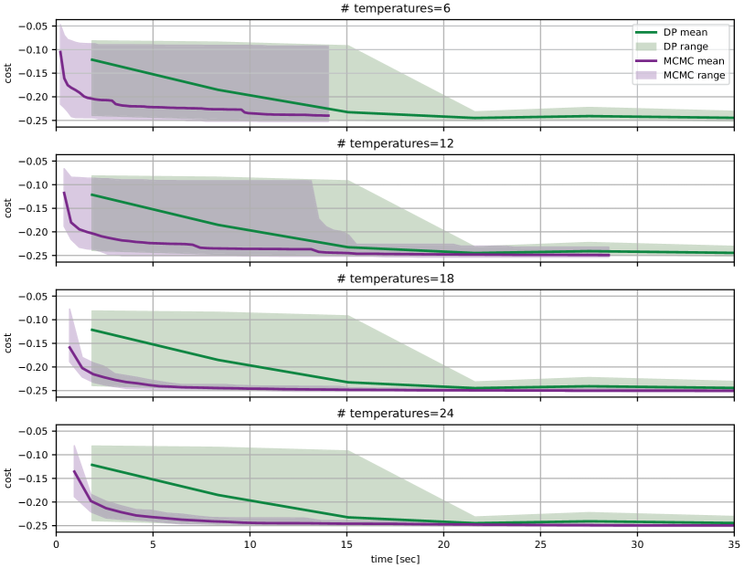
Figure 2 compares Algorithm 3 with the algorithm in [7], which exploits the piecewise-linear structure of the cost-to-go to efficiently represent and evaluate the value function and also to dynamically prune the search tree. Due to the need for exploration, this algorithm “protects” from pruning a random fraction of tree-branches (see [7] for details). Both algorithms used 6 CPU cores. For Algorithm 3, each core executed one sweep of the tempering algorithm and for the algorithm in [7], the 6 cores were used by BLAS to speedup matrix multiplication. Both algorithms were executed multiple times and the plots show the costs obtained as a function of run time. For Algorithm 3, the run time is controlled by the number of samples drawn. For the algorithm in [7], the run time is controlled by the number of vectors used to represent the value function. Both algorithms eventually discover comparable “optimal” solutions, but Algorithm 3 consistently finds a lower cost faster.
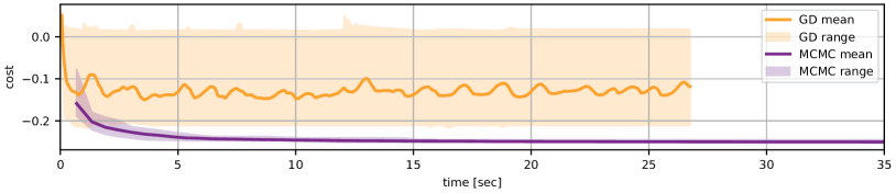
The top plot in Figure 3 compares Algorithm 3 with a gradient descent solver that minimizes the following continuous relaxation of the cost (5):
| (25) |
where the optimization variables are required to satisfy , . The global minimum of (25) would match that of (5), if we forced the to take binary values in . Otherwise, provides a lower bound for (6). We minimized (25) using the toolbox [2]. The results shown were obtained using Nesterov-accelerated adaptive moment estimation [2], with , which resulted in the best performance among the algorithms supported by [2]. The constraints on were enforced by minimum-distance projection into the constraint set. In general, gradient descent converges quickly, but to a local minima of (25) with cost higher then the minimum found by Algorithm 3 for (6); in spite of the fact that the global minima of (25) is potentially smaller than that of (6).
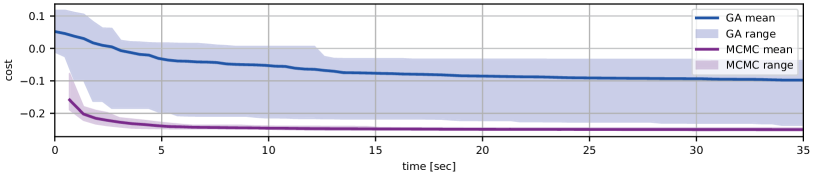
The bottom plot in Figure 3 compares Algorithm 3 with a genetic optimization algorithm that also resorts to stochastic exploration. This type of algorithm simulates a “population” of candidate solutions to the optimization (6), which evolves by mutation, crossover, and selection. We minimized (25) using the toolbox [1]. The results in Figure 3 used a population size , selection based on uniform ranking (which selects the best individuals with probability ), binary crossover (which combines the solution of the two parent with a single crossover point), a mutation rate of 10%, and a probability of mutation for each “gene” of 5%. These parameters resulted in the lowest costs we could achieve among the options provided by [1], but still significantly higher than the costs obtained with Algorithm 3.
References
- [1] https://github.com/wildart/Evolutionary.jl.
- [2] https://github.com/jacobcvt12/GradDescent.jl.
- Aadit et al. [2022] N. Aadit, A. Grimaldi, M. Carpentieri, L. Theogarajan, J. Martinis, G. Finocchio, and K. Y. Camsari. Massively parallel probabilistic computing with sparse Ising machines. Nature Electronics, 5(7):460–468, 2022.
- Bakker et al. [2019] C. Bakker, K. E. Nowak, and W. S. Rosenthal. Learning Koopman operators for systems with isolated critical points. In Proc. of the 58th IEEE Conf. on Decision and Contr., pages 7733–7739, 2019.
- Bengea and DeCarlo [2005] S. C. Bengea and R. A. DeCarlo. Optimal control of switching systems. Automatica, 41(1):11–27, 2005.
- Bevanda et al. [2021] P. Bevanda, S. Sosnowski, and S. Hirche. Koopman operator dynamical models: Learning, analysis and control. Annual Reviews in Control, 52:197–212, 2021.
- Blischke and Hespanha [2023] M. Blischke and J. P. Hespanha. Learning switched Koopman models for control of entity-based systems. In Proc. of the 62th IEEE Conf. on Decision and Contr., Dec. 2023.
- Brooks [1998] S. Brooks. Markov chain Monte Carlo method and its application. J. of the Royal Statistical Society: series D (the Statistician), 47(1):69–100, 1998.
- Brunton et al. [2016] S. Brunton, B. Brunton, J. Proctor, and J. N. Kutz. Koopman invariant subspaces and finite linear representations of nonlinear dynamical systems for control. PloS one, 11(2), 2016.
- Černỳ [1985] V. Černỳ. Thermodynamical approach to the traveling salesman problem: An efficient simulation algorithm. J. Opt. Theory and Applications, 45:41–51, 1985.
- Earl and Deem [2005] D. J. Earl and M. W. Deem. Parallel tempering: Theory, applications, and new perspectives. Physical Chemistry Chemical Physics, 7(23):3910–3916, 2005.
- Folkestad and Burdick [2021] C. Folkestad and J. W. Burdick. Koopman NMPC: Koopman-based learning and nonlinear model predictive control of control-affine systems. In Proc. of the IEEE Int. Conf. on Robot. and Automat. (ICRA), pages 7350–7356, 2021.
- Gelfand and Smith [1990] A. E. Gelfand and A. F. Smith. Sampling-based approaches to calculating marginal densities. J. of the American Statistical Assoc., 85(410):398–409, 1990.
- Geman and Geman [1984] S. Geman and D. Geman. Stochastic relaxation, Gibbs distributions, and the Bayesian restoration of images. IEEE Trans. on Pattern Anal. and Machine Intell., PAMI-6(6):721–741, 1984.
- Geyer [1991] C. J. Geyer. Markov chain Monte Carlo maximum likelihood. In Computing Science and Statistics: Proc. of the 23rd Symp. on the Interface, pages 156–163, 1991.
- Haseli and Cortés [2023] M. Haseli and J. Cortés. Modeling nonlinear control systems via Koopman control family: Universal forms and subspace invariance proximity, 2023. arXiv: 2307.15368.
- Hukushima and Nemoto [1996] K. Hukushima and K. Nemoto. Exchange Monte Carlo method and application to spin glass simulations. J. of the Physical Society of Japan, 65(6):1604–1608, 1996.
- Kemeny and Snell [1976] J. G. Kemeny and J. L. Snell. Finite Markov chains. Springer-Verlag, 1976.
- Kirkpatrick et al. [1983] S. Kirkpatrick, C. D. Gelatt Jr, and M. P. Vecchi. Optimization by simulated annealing. Science, 220(4598):671–680, 1983.
- Koopman [1931] B. O. Koopman. Hamiltonian systems and transformation in Hilbert space. Proc. of the National Academy of Sciences U.S.A, 17(5):315–318, 1931.
- Korda and Mezić [2018] M. Korda and I. Mezić. Linear predictors for nonlinear dynamical systems: Koopman operator meets model predictive control. Automatica, 93:149–160, 2018.
- Liu et al. [2023] Z. Liu, N. Ozay, and E. D. Sontag. Properties of immersions for systems with multiple limit sets with implications to learning Koopman embeddings, 2023. arXiv:2312.17045.
- Mauroy et al. [2020] A. Mauroy, Y. Susuki, and I. Mezić. Koopman operator in systems and control. Springer, 2020.
- Mezić [2005] I. Mezić. Spectral properties of dynamical systems, model reduction and decompositions. Nonlinear Dynamics, 41:309–325, 2005.
- Mohseni et al. [2022] N. Mohseni, P. L. McMahon, and T. Byrnes. Ising machines as hardware solvers of combinatorial optimization problems. Nature Reviews Physics, 4(6):363–379, 2022.
- Nüske et al. [2023] F. Nüske, S. Peitz, F. Philipp, M. Schaller, and K. Worthmann. Finite-data error bounds for Koopman-based prediction and control. Journal of Nonlinear Science, 33(1):14, 2023.
- Otto and Rowley [2021] S. E. Otto and C. W. Rowley. Koopman operators for estimation and control of dynamical systems. Annual Review of Control, Robotics, and Autonomous Systems, 4:59–87, 2021.
- Proctor et al. [2018] J. Proctor, S. Brunton, and J. N. Kutz. Generalizing Koopman theory to allow for inputs and control. SIAM J. on Applied Dynamical Syst., 17(1):909–930, 2018.
- Rothblum and Tan [1985] U. G. Rothblum and C. P. Tan. Upper bounds on the maximum modulus of subdominant eigenvalues of nonnegative matrices. Linear algebra and its applications, 66:45–86, 1985.
- Swendsen and Wang [1986] R. H. Swendsen and J.-S. Wang. Replica Monte Carlo simulation of spin-glasses. Physical Review Lett., 57(21):2607, 1986.
- Xu and Antsaklis [2004] X. Xu and P. Antsaklis. Optimal control of switched systems based on parameterization of the switching instants. IEEE Trans. on Automat. Contr., 49(1):2–16, 2004.