Unconstraining Multi-Robot Manipulation: Enabling Arbitrary Constraints in ECBS with Bounded Sub-Optimality
Abstract
Multi-Robot-Arm Motion Planning (M-RAMP) is a challenging problem featuring complex single-agent planning and multi-agent coordination. Recent advancements in extending the popular Conflict-Based Search (CBS) algorithm have made large strides in solving Multi-Agent Path Finding (MAPF) problems. However, fundamental challenges remain in applying CBS to M-RAMP. A core challenge is the existing reliance of the CBS framework on conservative “complete” constraints. These constraints ensure solution guarantees but often result in slow pruning of the search space – causing repeated expensive single-agent planning calls. Therefore, even though it is possible to leverage domain knowledge and design incomplete M-RAMP-specific CBS constraints to more efficiently prune the search, using these constraints would render the algorithm itself incomplete. This forces practitioners to choose between efficiency and completeness.
In light of these challenges, we propose a novel algorithm, Generalized ECBS, aimed at removing the burden of choice between completeness and efficiency in MAPF algorithms. Our approach enables the use of arbitrary constraints in conflict-based algorithms while preserving completeness and bounding sub-optimality. This enables practitioners to capitalize on the benefits of arbitrary constraints and opens a new space for constraint design in MAPF that has not been explored. We provide a theoretical analysis of our algorithms, propose new “incomplete” constraints, and demonstrate their effectiveness through experiments in M-RAMP.

1 Introduction
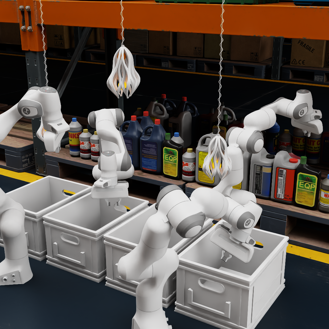
Teams of robots operating together in a shared workspace, can enhance the efficiency of existing systems and tackle challenges beyond the capabilities of a single robot. A key problem in multi-agent systems is Multi-Agent Path Finding (MAPF), the problem of finding efficient collision-free paths for multiple agents on graphs. Most existing multi-agent robotics research and MAPF applications have focused on simplistic systems like planar mobile robots in warehouses. Recently, interest in using more complex multi-agent systems to complete new tasks has increased. As exemplified in Figure 1, multi-robot-arm motion planning (M-RAMP) is particularly appealing due to its applicability for autonomous assembly, arrangement, and construction.
M-RAMP focuses on teams of high degrees of freedom (DoF) manipulators working in a shared workspace. Unlike typical MAPF applications in warehouses where hundreds of simple robots traverse a planar floor, M-RAMP typically has a few (e.g., less than ) robots, each having a rich configuration space (e.g., 7 DoF). Thus, M-RAMP contains unique challenges that standard 2D MAPF applications do not face. In particular, unlike 2D MAPF which assumes fast single-agent planners, M-RAMP single-agent planners need to search more complex configuration spaces without equally informed heuristics and require non-trivial collision checking. These differences may point to MAPF algorithms being inapplicable to M-RAMP. However, as recently shown, formulating M-RAMP as an application of MAPF to robot arms is an avenue for solving it efficiently.
The key insight in MAPF is to avoid planning in the composite configuration space for all agents by leveraging the semi-independence of agents. MAPF methods thus contain two main components: single-agent path finding and multi-agent collision resolution. From an abstract level, collisions in heuristic-search-based MAPF methods are prevented or resolved using constraints. Constraints, e.g., requiring agents to treat as moving obstacles or to avoid specific configurations at specific times, enable iterative planning of single agents to work towards a collision-free solution. Constraints have significant effects on the theoretical guarantees and practical results of methods.
Conflict-Based Search (CBS) (Sharon et al. 2015) famously applies constraints to prevent certain agents from occupying certain configurations at certain times to resolve conflicts. CBS’s constraints are complete (Definition 1) and enable CBS-based methods to yield optimal or bounded sub-optimal solutions. However, resolving collisions with these constraints may require many iterations practically causing CBS variants to often be slow to find solutions, especially when applied to domains with non-point robots.
Priority-based methods like Prioritized Planning (PP) (Erdmann and Lozano-Perez 1987) and PIBT (Okumura et al. 2019) prevent collisions by assigning agents priority and constraining lower-priority agents to avoid higher-priority agents. Priority constraints aggressively prune the search space and often make methods employing them fast. However, this comes at the cost of occasional failures in trivial instances requiring non-trivial coordination (e.g., two agents swapping positions in a hallway). Thus, these overly strong constraints may create methods that are “incomplete” in that they can fail to find solutions even when those exist.
We arrive at a central dilemma in MAPF: either gain efficiency by employing incomplete constraints or retain completeness at the cost of more computation. In challenging domains like M-RAMP, we ideally want to use arbitrary, likely incomplete, constraints to gain efficiency, but keep completeness. Walker, Sturtevant, and Felner (2020) proposed to support arbitrary constraints with completeness by adding them alongside complete constraints and then probabilistically deactivating them later on. Orthogonal to this approach, we discriminate between different types of arbitrary constraints to allow effective combinations of these, and guarantee bounded sub-optimal solution costs.
To this end, we design a framework that incorporates arbitrary constraints in CBS and identifies effective constraint types while guaranteeing completeness and bounded sub-optimality. We instantiate this framework with the algorithm Generalized ECBS, and propose new constraints111We highlight that our work only scratches the surface of constraint design and enables an entirely new design space for future research that can leverage different domain knowledge, or collected data, to construct new constraints. effective in M-RAMP. Across experiments with 4, 6, and 8 robot arms, we demonstrate how M-RAMP can be better solved with Generalized ECBS compared to complete methods (e.g., ECBS) and incomplete methods (e.g., Prioritized Planning, or ECBS with only incomplete constraints).
2 M-RAMP Problem Definition
Multi-Robot-Arm Motion Planning (M-RAMP) is the problem of finding low cost and collision-free paths for teams of manipulators (also named agents) from start configurations to goal configurations in a shared workspace. Let us consider as the configuration space of a single robot with DoF and the set of configurations not colliding with obstacles. A configuration is defined by assigning values (joint angles) to all the DoF. We denote the occupancy of a robot taking on the configuration as . Agents and are defined to be in conflict when .
A solution to the (discrete-time) M-RAMP problem is a set of single-agent paths . Each path222We use the shorthand to denote the configuration that takes at time according to when the context is clear. For other subscripts time is specified as needed. obeys , , all , and there are no conflicts between any pair at all time steps or interpolated transitions when those follow and . Our objective is to find the best valid solution in terms of time and motion (radians), minimizing the sum of costs .
3 Background
In practice, a common approach to solve M-RAMP is to plan in the composite state-space (i.e., considering all agents as a single high-dimensional agent) using sampling-based planners such as Rapidly exploring Random Trees (RRT) and its extensions (LaValle 1998; Kuffner and LaValle 2000; Shome et al. 2020). With more than one agent, solution quality sharply decreases, especially in clutter.
Another approach is to apply MAPF solvers for M-RAMP. Since naively applying algorithms like CBS (complete) or PP (incomplete) to arms may result in poor performance (Sec. 6.3), more nuanced approaches have been proposed. For example, CBS-MP (Solis et al. 2021) utilizes sparse roadmaps and modifies CBS constraints to prune the search space more but causes them to become incomplete.333Although the original paper claims completeness, we and its authors concluded otherwise; see Shaoul et al. (2024) for details. In this study, we aim to broaden CBS-based methods by supporting incomplete constraints while maintaining completeness. We first describe how manipulation planning can be solved using graph search and then describe the relevant CBS and ECBS work that our method builds on.
3.1 Manipulation Planning as Graph Search
One way to realize motion planning for a single agent is by encoding its configuration space in a graph and searching it for a collision-free shortest path from to via a sequence of edge-connected vertices. Vertices in this graph denote configurations , and edges are valid transitions between configurations. Since it is generally infeasible to enumerate all collision-free vertices and edges on these graphs for any reasonable , it is hard to compute informative heuristics. In this study, we employ methods to search these graphs as outlined by Cohen et al. (2011). Specifically, we use Weighted-A* for graph search to discourage excessive exploration of the vast search space, construct edges as discretized arm motions, and determine edge and vertex validity during the search.
Coordination between multiple agents can be done by augmenting single-agent graphs with a discretized time dimension, allowing waiting, and ensuring that no conflicts occur. We call conflicts during edge traversals edge conflicts, and vertex conflicts otherwise. By imposing this graph structure on the motions of individual robot arms, we can directly view M-RAMP as an application of MAPF to the robot-arm domain and employ algorithms like CBS to solve it.
3.2 Conflict-Based Search (CBS)
CBS is a popular complete and optimal MAPF solver that employs a low-level single-agent planner and a high-level constraint tree (CT) to resolve conflicts (Sharon et al. 2015). Given a set of paths, CBS detects conflicts in pairs of agents and resolves them by applying constraints.
Concretely, a CT node contains a set of paths , one for each agent, which satisfy a set of constraints . CBS prioritizes CT nodes in an OPEN queue by their cost . CBS initializes OPEN with a root CT node with no constraints and individually optimal paths. CBS proceeds iteratively, taking the best node and checking for conflicts. If there are no conflicts, it has found a valid solution and terminates. If not, it picks a conflict to resolve. CBS resolves conflicts by applying constraints to the participating agents, one for each, and generates two successor CT nodes with agents replanned to satisfy the new constraint.
3.3 Enhanced Conflict-Based Search (ECBS)
ECBS (Barer et al. 2014) differs from CBS in its use of a focal list (Pearl and Kim 1982), a mechanism for arbitrarily prioritizing a portion of OPEN while guaranteeing bounded sub-optimality, in the high- and low-level search. In the high-level search, ECBS defines
where and is a lowerbound on the cost of path . ECBS chooses the CT node with the least conflicts, , with being the conflict set identified in . This yields solutions with cost at most , with the optimal sum of costs, that are generally found much faster than CBS.
Crucially for guaranteeing completeness in CBS and its variants, the constraints that they employ must be complete (otherwise known as mutually disjunctive). We adopt the following definition from Li et al. (2019).
Definition 1 (Complete Constraints).
A constraint is complete if, when used to resolve a conflict between and via imposing constraints and on the agents respectively, there do not exist any two conflict-free paths for and with violating and violating .
For example, vertex constraints (Sec. 4) are complete. Let vertex constraints and be imposed on and to resolve a conflict between and at time . Any path for that violates must include at time . mirrors. Therefore, these paths will always lead to a collision at time , and by Def. 1, vertex constraints are complete.
4 Constraints
It is often intuitive to formulate effective constraints that accelerate the search but are incomplete. Historically, methods either accepted this incompleteness in favor of the gains in efficiency it practically provided or agreed to bargain runtime for the theoretical guarantee of completeness. In this work, we allow for the use of arbitrary constraints in the CBS framework while guaranteeing completeness and bounding sub-optimality.
This section describes the constraints commonly used in MAPF and introduces new constraints. In the following definitions, we consider the constraints and that are imposed to resolve a conflict between agent and . The time of conflict is , at which the robots took on the configurations and with the associated collision point . For brevity, we describe the resolution of vertex conflicts and note that edge conflicts in follow identically. Additionally, we only describe with mirroring it accordingly, similar to how CBS resolves conflicts with symmetric pairs of constraints, one per agent.
4.1 Existing Constraints
The most commonly used constraints in the CBS framework are vertex and edge constraints. These are the original domain-agnostic constraints in CBS that guarantee completeness.
Definition 2 (Vertex Constraint).
forbids from taking on the configuration at time .
The main drawback of these constraints is their small effect on the search space: preventing agents from occupying exactly one configuration (vertex) at a time. We would prefer to remove larger subsets of the search space when resolving a conflict, but this may come at the cost of completeness. For example, instead of solely avoiding a single configuration, CBS-MP avoids the entire volume occupied by the other agent. We name this an “avoidance” constraint.
Definition 3 (Avoidance Constraint).
forbids from colliding with the volume at time .
Interestingly as we show in Figure 2, this is not complete.
Arguably the most popular incomplete constraint, used by PP and PBS (Ma et al. 2019), is “priority.”
Definition 4 (Priority Constraint).
forbids from colliding with as it moves along its current path . Formally, forbids from taking on at time if .
4.2 New Constraints
In M-RAMP, a collision point is associated with a conflict. A natural choice for a constraint then is restricting agents from re-occupying at . Adding a margin, we call these sphere constraints.
Definition 5 (Sphere Constraints).
forbids from colliding with a spherical obstacle with a radius centered at the collision point at time . i.e., the set is disallowed at time .
Depending on the collision checker of choice, sphere constraint satisfaction can be cheap to compute and an effective way to resolve conflicts quickly. With a non-zero radius, sphere constraints are incomplete (see Fig. 2), however, as (i.e., as the constraint becomes the point itself) a sphere constraint becomes complete. We provide a quick proof. Let and be any two configurations violating a symmetric “point constraint.” Formally, and . Thus, and “point constraints” are complete by Definition 1.
Additionally, we add flexibility to priority constraints by restricting priorities to a single time .
Definition 6 (Step-Priority Constraints).
Let be the configuration of at time in its current path . forbids from colliding with at time .
Step-priority constraints are different from avoidance constraints. When avoids , it is not allowed to collide with the original conflicting configuration of . Step-priority disallows from colliding with the updated configuration of according to its most recent path; therefore, this constraint adaptively changes with .
5 Algorithmic Approach
Generalized ECBS allows CBS variants to handle arbitrary constraints while keeping completeness and bounded sub-optimality guarantees. We first describe a simple and inefficient method named Arbitrary Constraint ECBS (AC-ECBS) for incorporating arbitrary constraints into ECBS. We prove that AC-ECBS is complete and bounded sub-optimal and lay the theoretical foundation for Generalized ECBS. We then introduce Generalized ECBS and explain how it overcomes the efficiency challenges plaguing AC-ECBS by lazily expanding CT nodes and prioritizing promising constraint types.
5.1 Arbitrary Constraint ECBS with Guarantees
Given arbitrary constraint types, i.e., different constraint options to resolve the same conflict (for example, when including small sphere, large sphere, and avoidance constraints), AC-ECBS is identical to ECBS except that it generates child CT nodes on each expansion. nodes are generated using the arbitrary constraints and the additional two with complete (vertex/edge) constraints.
Lemma 1.
AC-ECBS is complete.
Proof.
In ECBS, a solution is found in an iterative process. Starting from a root CT node , CT nodes are branched to two child nodes by adding a single complete (vertex or edge) constraint to each and queuing them in a high-level OPEN list. In AC-ECBS, we know that for each expanded CT node, there always exist two child nodes that have been created by the addition of only complete constraints. Define a “Complete Subtree” . Therefore, the high-level OPEN list of AC-ECBS is a superset of the OPEN of ECBS and therefore includes CT nodes guaranteed to lead to a solution by continuing to resolve conflicts in them with complete constraints. Thus, additional child nodes in CT expansions does not affect the completeness of ECBS. ∎
Lemma 2.
AC-ECBS is bounded sub-optimal with a bound identical to ECBS.
Proof.
As before, let the lower-bound of a CT node be . From Lemma 1, the high-level OPEN in AC-ECBS is always a superset of some ECBS OPEN, which we’ll name . Therefore, the lower bound . In ECBS, we have by construction. Thus, and all nodes in the AC-ECBS FOCAL list have bounded sub-optimal costs . ∎
5.2 Generalized ECBS
Although AC-ECBS can handle arbitrary constraints, it suffers from needing to generate all successors at every CT expansion. Furthermore, certain constraints may be more appropriate for certain planning problems (e.g., smaller constraints are better than larger ones in tight coordination), and we would like the algorithm to adapt to such a need. We tackle both of these problems with Generalized ECBS. Our key idea is to use lazy expansions to ease computational work and multiple focal queues to adaptively prioritize constraint types. Algorithm 1 describes Generalized ECBS.
Lazy CT Expansion
Imagine we are given a node with some conflicts that need to be resolved. In AC-ECBS, we apply the constraints and query that many low-level planning calls before inserting these successor nodes into OPEN and FOCAL. Drawing inspiration from work on lazy planning, where nodes are generated during the search and checks for their validity are deferred (Mukherjee, Aine, and Likhachev 2022; Haghtalab et al. 2018), we instead generate all nodes, each with an extended constraint set (Line 1), but delay the low-level planning calls (Line 1). Unlike common lazy approaches that assume fast node generation, our successor generation requires replanning and is expensive. Thus, we reuse parent values (e.g., the sum of costs and number of conflicts) in child nodes and insert them into the queue using the priority derived from these approximate values. Now, when choosing a node for expansion, if it is an approximate node we only then call the low-level planner to get the updated paths and re-queue it (Line 1).
When adding lazy evaluations to AC-ECBS directly, successor nodes are indistinguishable in terms of their cost and conflict count values (see Fig. 3(a)), causing child nodes to be prioritized in an uninformed manner. We can solve this issue using multiple focal queues.
Multiple Focal Queues
The main problem with one focal queue is that it can only be sorted with one priority function, making it hard to distinguish between lazy successor nodes with the same approximate values (i.e., a copy of their parent values). Additionally, designers creating these constraints may have priors on certain constraints being more useful than others. Inspired by Phillips et al. (2015), we can tackle both of these issues by generalizing CBS to have multiple FOCAL queues (Line 1), each sorted by their priority function. Each priority function can distinguish between identical lazy successor nodes and incorporate external domain knowledge by prioritizing specific constraint types.
Concretely, given arbitrary constraint types (excluding the complete edge/vertex constraints), we initialize FOCAL queues. Each uses to sort CT nodes lexicographically by (Line 1). That is, primarily according to the number of conflicts in the paths of , breaking ties according to the sum of costs and (one minus) the density of constraints of type in .
We note that arbitrary priority functions are possible and encourage incorporating domain knowledge here too. We found that this worked well in practice.
Choosing Between Queues
Given multiple FOCAL queues and an OPEN queue, we need to choose which queue to pick to decide our next CT node to expand. A simple approach used before in single-agent works is to evenly rotate between all the queues (Aine et al. 2016).
However, some constraints may prove to be more effective in different parts of the search, and we would like the algorithm to dynamically prioritize those. We can use Dynamic Thompson Sampling (DTS) as described in Phillips et al. (2015) to define a selection mechanism among all the queues that get updated during the search. As seen in Algorithm 1, each time an un-evaluated CT node is considered from , it is evaluated and its true conflict set is computed (line 1). If it has fewer conflicts than in inherited from its parent, then this is prioritized. Otherwise, it is penalized (lines 1 and 1). Internally, DTS keeps a beta distribution parameterized by . Upon each penalty or reward, DTS increments or , skewing the distribution towards or respectively. After each update operation, a value is sampled from all , and the index of the newly activated is set to . DTS dampens the effects of the history on updates via a parameter , keeping the sum always. In our experiments .
Putting it all together
We now describe Generalized ECBS with both these components (lazy expansion and multiple FOCAL queues) in a quick example (Fig. 3). Imagine working in a 3D manipulation domain and designing types of constraints and to resolve conflicts. We again note that we always have access to at least one type of “complete” constraint (e.g., regular vertex/edge constraint). Generalized ECBS creates 4 queues; OPEN along with , , . is sorted by conflict count and each is sorted as described previously. We could initialize our DTS beta distributions with a uniform prior () or instead bias them based on experience. In this example, DTS initially favors .
In the beginning, we generate the root node and collect all collisions. Instead of generating the successor nodes by calling low-level planners for each constraint, we generate the nodes without replanning agents and insert them into OPEN and all FOCAL queues (Fig. 3(a)). Due to the bias, we sample and choose its best node (Fig. 3(b)). Here the node contains approximate values, so we call the low-level planners to replan with the constraint and re-queue the node (Fig. 3(c)). We reward the DTS sampling distribution since the number of conflicts decreased. We now repeat and sample . If the same node is picked (Fig. 3(c)), it is fully evaluated which means we generate the lazy successors (Fig. 3(d)). We repeat this process iteratively until we reach a conflict-free solution or timeout. We note that Generalized ECBS is complete and bounded sub-optimal for the same reasons outlined in Section 5.1.
6 Experiments
To evaluate the performance of Generalized ECBS, we created three test scenarios similar to real-world multi-arm manipulation problems that M-RAMP algorithms would be expected to solve (Fig. 4). Our tests feature closely interacting manipulators and complex obstacle landscapes. The results suggest that effectively capitalizing on the benefits of incomplete constraints helps solve M-RAMP problems faster.
| 8 Robots | Succ. (%) | Runtime (s) | Cost (rad) |
|---|---|---|---|
| ECBS | 48% | 17.7 19.46 | 38.9 7.30 |
| ECBS-A | 78% | 13.1 12.60 | 39.9 6.64 |
| ECBS-P | 78% | 13.2 12.57 | 39.9 6.63 |
| ECBS-S | 76% | 15.8 15.97 | 40.5 7.15 |
| ECBS-LS | 10% | 8.6 10.20 | 30.4 2.49 |
| ECBS-XLS | 4% | 3.2 1.78 | 28.5 1.04 |
6.1 Experimental Setup
We set up planning problems, each characterized by start-goal pairs. Single-agent configurations and were randomly chosen from a set of task-relevant poses (e.g., pick poses inside different bins) for each agent and verifying the validity of and . This task dependence in the problem construction promotes high levels of interaction between agents, similar to that in realistic multi-arm manipulation tasks.
To shed light on the scalability of our algorithm, we vary the number of robots and the levels of interaction between experiments, as illustrated in Figure 4. We include two scenarios resembling real-world planning tasks: pick-and-place with robots and shelf rearrangement with robots. Both showcase significant clutter and proximity between agents. We also include a relatively open environment with robots with a single obstacle between them.
Aiming to verify the ability of Generalized ECBS to handle a large number of incomplete constraints, for each vertex or edge conflict in our evaluation, we generate avoidance, step-priority, complete (vertex/edge), and three types of sphere constraints with radii , , and cm. We set an initial DTS bias towards the smaller sphere constraints.
Each robot in our experiments is a Franka Panda manipulator with 7 DoF. The experiments were conducted on an Intel Core i9-12900H laptop with 32GB RAM (5.2GHz). We implemented all algorithms in C++, used the MoveIt!2 (Coleman et al. 2014) software for interacting with manipulators, and Flexible Collision Library (FCL) (Pan, Chitta, and Manocha 2012) for collision checking.
6.2 Evaluated Methods
We compare Generalized ECBS to ubiquitous methods commonly used in motion planning for robotics manipulators, as well as to popular MAPF algorithms. We choose to include RRT-Connect and PRM as these are arguably the most frequently used algorithms in planning for manipulation. These algorithms plan for all agents jointly, treating the team of robotic manipulators as a single composite agent. We use the OMPL (Sucan, Moll, and Kavraki 2012) implementation.
We additionally include results from MAPF planners. We include PP, CBS-MP, CBS, and ECBS, as well as Generalized CBS and Generalized ECBS. Generalized CBS differs from Generalized ECBS in that it does not assume access to conflict counts in high-level and low-level nodes, and as such does not prioritize nodes based on this information. All algorithms employ Weighted-A* as their single-agent planner with a weight444Our heuristic underestimates the cost to go in radians, and edges are unit cost. The weight scales the heuristic value to match the cost of edge transitions and inflates it. of and an joint-angle heuristic function. Adaptive motion primitives are of degrees in individual joints when the end-effector is closer than cm to its goal location. Otherwise, degrees in the lower joints. Edge transitions are of uniform cost and take a single timestep. The sub-optimality bound of ECBS and Generalized ECBS is set to 1.3, and for all FOCAL lists for Generalized CBS to . Our implementation of CBS-MP differs slightly from the original in that, here, agents plan on implicit graphs and not on precomputed roadmaps to compare all search algorithms on the same planning representation.
| 8 Robots | Succ. (%) | Runtime (s) | Cost (rad) |
|---|---|---|---|
| ECBS | 48% | 17.7 19.4 | 38.9 7.3 |
| AC-ECBS | 38% | 27.4 17.2 | 38.5 7.3 |
| AC-ECBS-L | 54% | 18.1 17.2 | 40.6 7.2 |
| Gen-ECBS | 84% | 18.8 16.3 | 41.2 6.9 |
We evaluate algorithm scalability and solution quality per scene by reporting mean and standard deviation for planning time and solution cost across problems, along with the success rate for each algorithm. Algorithms are allotted seconds for planning; exceeding this time is considered a failure. Solution cost is measured by the total joint motion in radians. All solutions undergo post-processing with a simple shortcutting algorithm which sequentially shortens each agent’s solution path without introducing conflicts by replacing segments with linear interpolations while avoiding obstacles and other agents. This standard shortcutting method is commonly used to refine paths generated by sampling-based planners (Choset et al. 2005).

| 8 Robots | Success (%) | Runtime (sec) | Cost (rad) |
|---|---|---|---|
| Gen-ECBS | 84% | 18.8 16.39 | 41.2 6.93 |
| Gen-CBS | 34% | 20.9 17.38 | 36.9 6.15 |
| ECBS | 48% | 17.7 19.46 | 38.9 7.30 |
| CBS | 18% | 23.3 23.03 | 35.0 6.08 |
| PP | 52% | 14.5 9.64 | 39.0 6.48 |
| RRT-Con | 0% | - | - |
| PRM | 0% | - | - |
| CBS-MP | 36% | 15.2 15.19 | 36.9 5.93 |

| 6 Robots | Success (%) | Runtime (sec) | Cost (rad) |
|---|---|---|---|
| Gen-ECBS | 84% | 7.4 11.43 | 31.8 5.01 |
| Gen-CBS | 42% | 15.3 15.19 | 29.4 4.77 |
| ECBS | 70% | 11.6 10.26 | 31.2 5.26 |
| CBS | 22% | 14.1 18.59 | 29.9 5.12 |
| PP | 72% | 12.7 14.41 | 31.5 4.68 |
| RRT-Con. | 84% | 1.4 1.71 | 103.9 35 |
| PRM | 18% | 17.2 20.61 | 131.6 108 |
| CBS-MP | 54% | 15.9 18.44 | 30.3 5.16 |
| 4 Robots | Success (%) | Runtime (sec) | Cost (rad) |
|---|---|---|---|
| Gen-ECBS | 98% | 9.5 11.10 | 23.2 3.66 |
| Gen-CBS | 60% | 15.3 15.57 | 21.4 2.91 |
| ECBS | 86% | 12.5 15.08 | 22.6 3.61 |
| CBS | 28% | 9.1 9.61 | 20.4 2.89 |
| PP | 88% | 11.4 13.98 | 22.9 3.51 |
| RRT-Con. | 32% | 10.9 10.00 | 60.5 19.55 |
| PRM | 2% | 13.3 0.0 | 78.9 0.0 |
| CBS-MP | 68% | 13.9 14.06 | 21.7 2.99 |
6.3 Experimental Results
Table 1 highlights the mercurial behavior of incomplete constraints when substituting them in ECBS in place of complete constraints. When effective, incomplete constraints like avoidance, step-priority, or sphere can improve success rates, showcasing how these constraints can effectively prune the search space. However, it may not be clear in some domains if constraints are overly pruning. We see that increasing the sphere constraint radius from 5cm (ECBS-S) to 15cm (ECBS-LS) dramatically reduces the success rate in our 8-arm scene as the search space becomes overly constrained. Thus constraints must be used intelligently to provide consistent benefits or risks needing to be re-evaluated for utility in every scenario.
This motivates trying out all the constraints at once with AC-ECBS as described in Section 5.1. AC-ECBS in Table 2 demonstrates how naively incorporating all these constraints within the ECBS framework leads to a larger runtime and a lower success rate due to the large branching factor. Using lazy expansions (AC-ECBS-L) improves performance compared to AC-EBCS but marginally against regular ECBS. By employing multiple queues and adaptively prioritizing constraint types, Generalized ECBS can effectively capitalize on the benefits of incomplete constraints and achieve a significant improvement in planning time and success rate.
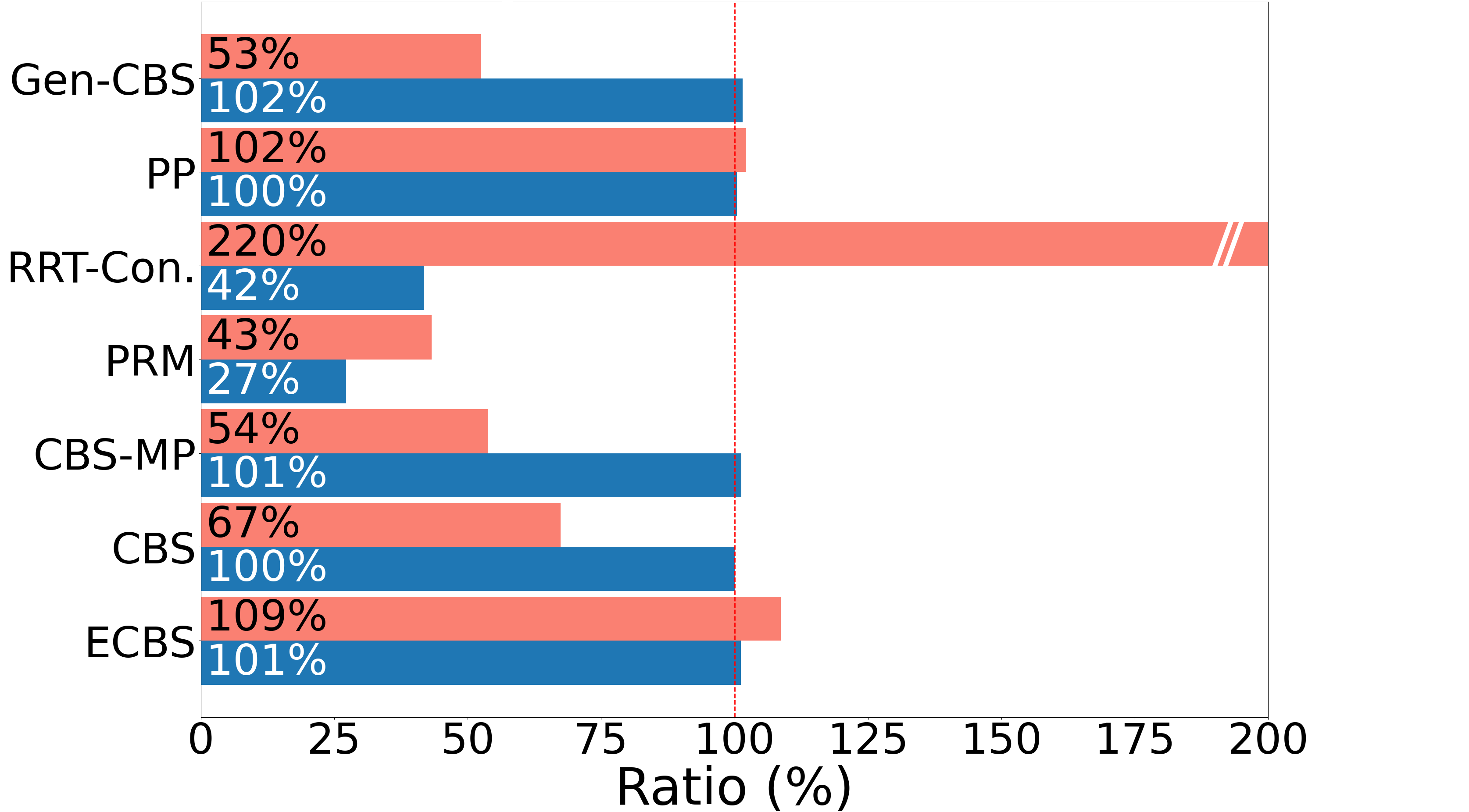
We compare Generalized ECBS with other standard approaches to M-RAMP in Figure 4 and see that it has a higher success rate than all other baselines. For 4 and 6 robots, sampling-based methods (PRM, RRT-Connect) impressively succeed in finding solutions to some problems, however, suffer from poor path cost and overall success rate. With 8 robots, these methods fail, showing how MAPF reasoning (rather than composite space planning) is preferred. In this challenging scenario, it is particularly interesting to compare Generalized ECBS with Prioritized Planning (PP) which has severe incomplete constraints, and with ECBS which has only complete constraints. We see that Gen-ECBS has a higher success rate than PP, implying that the priority constraints are too strict. However, we see that just complete constraints, ECBS, also performs worse than Generalized ECBS. This highlights how using multiple incomplete and complete constraints is better than either by themselves.
7 Conclusion
Existing MAPF works are ubiquitous in 2D grid worlds, but may struggle in more realistic domains like Multi-Robot-Arm Motion Planning (M-RAMP). A key factor in their success is the type of constraints they use. We observed that in current frameworks, methods either apply complete constraints and are theoretically complete and bounded sub-optimal but slow, or apply stronger constraints and are fast but incomplete. Practitioners in today’s paradigm are thus forced to pick between slow methods with guarantees or fast methods that can fail on solvable instances.
We bridge this gap with Generalized-ECBS, which enables using arbitrary incomplete constraints without giving up completeness or bounded sub-optimality. Gen-ECBS uses lazy expansions, multiple focal queues, and dynamic prioritization to effectively use multiple constraints for a higher and more consistent success rate. In our experiments, we observed that Generalized-ECBS is effective in high-dimensional M-RAMP with a few simple constraints. Our proposed approach is domain-agnostic, and we are excited about the possibilities that it opens to future research in MAPF and multi-arm manipulation.
Acknowledgements
The work was supported by the National Science Foundation under Grant IIS-2328671 and the CMU Manufacturing Futures Institute, made possible by the Richard King Mellon Foundation.
References
- Aine et al. (2016) Aine, S.; Swaminathan, S.; Narayanan, V.; Hwang, V.; and Likhachev, M. 2016. Multi-Heuristic A*. The International Journal of Robotics Research, 224–243.
- Barer et al. (2014) Barer, M.; Sharon, G.; Stern, R.; and Felner, A. 2014. Suboptimal Variants of the Conflict-Based Search Algorithm for the Multi-Agent Pathfinding Problem. In International Symposium on Combinatorial Search, 19–27.
- Choset et al. (2005) Choset, H.; Lynch, K. M.; Hutchinson, S.; Kantor, G. A.; and Burgard, W. 2005. Principles of Robot Motion: Theory, Algorithms, and Implementations. MIT press.
- Cohen et al. (2011) Cohen, B. J.; Subramania, G.; Chitta, S.; and Likhachev, M. 2011. Planning for Manipulation With Adaptive Motion Primitives. In IEEE International Conference on Robotics and Automation, 5478–5485.
- Coleman et al. (2014) Coleman, D.; Sucan, I.; Chitta, S.; and Correll, N. 2014. Reducing the Barrier To Entry of Complex Robotic Software: a MoveIt! Case Study. arXiv preprint arXiv:1404.3785.
- Erdmann and Lozano-Perez (1987) Erdmann, M.; and Lozano-Perez, T. 1987. On Multiple Moving Objects. Algorithmica, 477–521.
- Haghtalab et al. (2018) Haghtalab, N.; Mackenzie, S.; Procaccia, A.; Salzman, O.; and Srinivasa, S. 2018. The Provable Virtue of Laziness In Motion Planning. In International Conference on Automated Planning and Scheduling, 106–113.
- Kuffner and LaValle (2000) Kuffner, J.; and LaValle, S. 2000. RRT-Connect: An Efficient Approach to Single-Query Path Planning. IEEE International Conference on Robotics and Automation.
- LaValle (1998) LaValle, S. 1998. Rapidly-Exploring Random Trees: A New Tool For Path Planning. Research Report 9811.
- Li et al. (2019) Li, J.; Surynek, P.; Felner, A.; Ma, H.; Kumar, T. S.; and Koenig, S. 2019. Multi-Agent Path Finding for Large Agents. In AAAI Conference on Artificial Intelligence, 7627–7634.
- Ma et al. (2019) Ma, H.; Harabor, D.; Stuckey, P. J.; Li, J.; and Koenig, S. 2019. Searching with Consistent Prioritization for Multi-Agent Path Finding. In AAAI Conference on Artificial Intelligence, 7643–7650.
- Mukherjee, Aine, and Likhachev (2022) Mukherjee, S.; Aine, S.; and Likhachev, M. 2022. ePA*SE: Edge-based Parallel A* for Slow Evaluations. In International Symposium on Combinatorial Search, 136–144.
- Okumura et al. (2019) Okumura, K.; Machida, M.; Défago, X.; and Tamura, Y. 2019. Priority Inheritance with Backtracking for Iterative Multi-agent Path Finding. In International Joint Conference on Artificial Intelligence, 535–542.
- Pan, Chitta, and Manocha (2012) Pan, J.; Chitta, S.; and Manocha, D. 2012. FCL: A General Purpose Library for Collision and Proximity Queries. In IEEE International Conference on Robotics and Automation, 3859–3866.
- Pearl and Kim (1982) Pearl, J.; and Kim, J. H. 1982. Studies in Semi-Admissible Heuristics. IEEE Transactions on Pattern Analysis and Machine Intelligence, 392–399.
- Phillips et al. (2015) Phillips, M.; Narayanan, V.; Aine, S.; and Likhachev, M. 2015. Efficient Search with an Ensemble of Heuristics. In International Conference on Artificial Intelligence, 784–791.
- Shaoul et al. (2024) Shaoul, Y.; Mishani, I.; Likhachev, M.; and Li, J. 2024. Accelerating Search-Based Planning for Multi-Robot Manipulation by Leveraging Online-Generated Experiences. In International Conference on Automated Planning and Scheduling.
- Sharon et al. (2015) Sharon, G.; Stern, R.; Felner, A.; and Sturtevant, N. R. 2015. Conflict-Based Search for Optimal Multi-Agent Pathfinding. Artificial Intelligence, 40–66.
- Shome et al. (2020) Shome, R.; Solovey, K.; Dobson, A.; Halperin, D.; and Bekris, K. E. 2020. dRRT*: Scalable and Informed Asymptotically-Optimal Multi-Robot Motion Planning. Autonomous Robots, 443–467.
- Solis et al. (2021) Solis, I.; Motes, J.; Sandström, R.; and Amato, N. M. 2021. Representation-Optimal Multi-robot Motion Planning Using Conflict-based Search. IEEE Robotics and Automation Letters, 4608–4615.
- Sucan, Moll, and Kavraki (2012) Sucan, I. A.; Moll, M.; and Kavraki, L. E. 2012. The Open Motion Planning Library. IEEE Robotics and Automation Magazine, 72–82.
- Walker, Sturtevant, and Felner (2020) Walker, T. T.; Sturtevant, N. R.; and Felner, A. 2020. Generalized and Sub-Optimal Bipartite Constraints for Conflict-Based Search. In AAAI Conference on Artificial Intelligence, 7277–7284.