Towards Predicting Collective Performance in Multi-Robot Teams

Abstract

The increased deployment of multi-robot systems (MRS) in various fields has led to the need for analysis of system-level performance. However, creating consistent metrics for MRS is challenging due to the wide range of system and environmental factors, such as team size and environment size. This paper presents a new analytical framework for MRS based on dimensionless variable analysis, a mathematical technique typically used to simplify complex physical systems. This approach effectively condenses the complex parameters influencing MRS performance into a manageable set of dimensionless variables. We form dimensionless variables which encapsulate key parameters of the robot team and task. Then we use these dimensionless variables to fit a parametric model of team performance. Our model successfully identifies critical performance determinants and their interdependencies, providing insight for MRS design and optimization. The application of dimensionless variable analysis to MRS offers a promising method for MRS analysis that effectively reduces complexity, enhances comprehension of system behaviors, and informs the design and management of future MRS deployments.

I Introduction

Distributed multi-robot systems (MRS) are increasingly utilized across a broad spectrum of fields, including search and rescue [Murphy2004Human-robot, Queralta2020], surveillance [Doitsidis2012], mapping [Deutsch2016SLAM], and reconstruction [Dong2019Reconstruction]. These systems are highly valued for their scalability, resilience [Zhou2023], redundancy, and efficiency. Many successful algorithms have addressed challenges in distributed MRS, such as coordinating robot movements, managing uncertainties, and optimizing search efficiency. Typically, these algorithms demonstrate strong performance in specific environments with particular sets of parameters, such as swarm size, task size, perception capabilities. This specificity is understandable, given the high-dimensional nature of the parameter space and the vast number of possible parameter combinations, which can be either continuous or discrete. However, system designers face the challenge of identifying the right set of parameters and forecasting system performance when deploying MRS algorithms in unknown environments. Consequently, there is a need for an empirical model that correlates system performance with system parameters.

Building such a model is a formidable task filled with numerous questions. Does a quantifiable relationship between these variables exist? How accurate can the predictions be? Can this model be generalized across different scenarios? These are critical inquiries that guide the development of a reliable and effective predictive model for MRS performance. Given the vast array of algorithms in distributed MRS, it is impractical to prove that any single model could be universally applicable. Therefore, we will focus our analysis on the application of Multi-Robot Multi-Target Tracking (MR-MTT), one of the most important problem in MRS, and demonstrate its effectiveness in this context.

I-A MR-MTT

MR-MTT is an area where the complexity and diversity of operational scenarios are particularly pronounced [robin2016multi]. MR-MTT has many potential applications, including surveillance, search and rescue, environmental monitoring, and industrial automation. In MR-MTT, a team of robots coordinate to monitor a group of targets in a given environment. We assume that the robots operate in a known area where the number of targets is initially completely unknown (e.g., the robots know the blueprint map of a building but not how many people are inside). This problem is challenging due to: 1) The potential mobility of targets, whose motion patterns are typically, at best, partially known. 2) The possibility of misidentification or missed detection of targets, coupled with the uncertainty and variation in their number over time. 3) The robots’ limited access to environmental information, constrained by their sensor field of view (FoV) and communication capabilities.

In addressing the challenges of MR-MTT, our previous work [dames2020distributed, xin2022comparing, xin2024comparison] introduced algorithms based on probabilistic search methods, which are particularly well-suited to target tracking problems given the significant noise present in the robots’ sensors. Rather than providing worst-case guarantees, this approach evaluates the probabilities of target detection [robin2016multi, stone2013bayesian]. This approach often involves mapping these probabilities onto the environment, creating a ‘heatmap’ of sorts that guides the search effort. The primary reason for this methodology is the frequent lack of resources (such as robots or time) to address the worst-case scenario (ensuring the detection of a target if it is present [chung2018gues]). However, it can also represent a strategic compromise between efficiency and the likelihood of encountering particularly challenging situations. Strategies may involve prioritizing specific areas based on their probability scores or dynamically allocating resources as the search progresses.

The inherent complexity of MR-MTT, arising from a vast variable space that includes the number of robots, number of targets, perception capabilities, motion models, and constraints such as communication and environment, makes it challenging to identify an optimal set of parameters for improving performance when reusing MR-MTT algorithms. Similarly, these constraints and the extensive variable space complicate the comparison and analysis of specific algorithms.

I-B Dimensionless Variables

We consider to use dimensionless variables, because it offers a method to scale down the complexity and preserve the essence of the problem. And it often allows for the derivation of universal solutions that are independent of the specifics of the system [Maltbaek1980, Thomas2007, Xie2022]. One example of a dimensionless variable is the Reynolds number. Originating from the study of turbulent Rayleigh–Bénard convection, a classic problem in fluid mechanics, the Reynolds number is defined as a power-law relation of four physical quantities: fluid density, average fluid velocity, pipe diameter, and dynamic fluid viscosity. The value of the Reynolds number dictates whether the flow will be turbulent or laminar and works across a range of length scales, fluids, etc.

The concept of dimensionless variables plays an essential role in the analysis of physical systems, allowing for normalized comparisons and simplifying mathematical models. Two systems may appear different due to varying units or scales, but they may be identical or similar when expressed in dimensionless form. In our case, this can reveal fundamental characteristics of the MRS, such as the ratio of robot number to target number, which could influence system task allocation, efficiency, reliability, and cost-effectiveness. Thus, we investigate to model the MRS performance based on dimensionless variables to understand, compare and optimize MRS algorithms.

I-C Approach

To study trends in the performance of MRSs, we will utilize datasets from our previous work [dames2020distributed, xin2022comparing, xin2024comparison], which all address the problem of distributed control for MR-MTT. We will utilize the data from these papers and run additional studies to obtain representative data that includes variations in the number of robots, the number of targets, and the FoV of the sensors. We measure the performance of the team using two metrics. The first is the Optimal SubPattern Assignment (OSPA) metric [Schuhmacher2008Metric], a commonly used metric in the MTT community that measures the average error of all targets. The second is the Exploration Inefficiency (EI), which measures the exploration progress. With either metric, we typically see a rapid initial decline that approaches an asymptote as exploration progresses.

Based on this observation, we fit two different models from the exponential family: an exponential and a sigmoid. We note that the parameters of these models depend upon the parameters of the robot team and the task, e.g., number of robots or number of targets. However, there is not a clear trend for how changes in any single team/task parameter affect team performance. The primary novelty in our work is the creation of a dimensionless variable that effectively describes these trends in the exponential function parameters as team/task parameters vary. More specifically, we utilize the Buckingham Pi Theorem from the high-dimensional variable space and co-optimize the structure of the dimensionless variable and its relationship to the parameters in the exponential models. This allows us to interpolate and extrapolate between existing samples to accurately predict team performance in novel scenarios. It also provides insight into the team/task parameters that most affect team performance, allowing practitioners to create teams to achieve certain levels of performance. Finally, we demonstrate that the structure of the dimensionless variable is consistent across exponential models, performance metrics, and control algorithms, indicating that the parameter provides insight into a broad range of scenarios.

I-D Contributions

The key contributions of this paper are: 1) We identify key parameters $\theta$ that relate to the ability of an MRS to complete an MR-MTT task. 2) We develop an algorithmic pipeline that co-optimizes the structure of a dimensionless variable $\Pi(\theta)$ (as a function of the parameters $\theta$) and the relationship between $\Pi$ and key indicators of MR-MTT success. 3) We demonstrate that our pipeline is able to accurate predict MR-MTT performance in scenarios outside of the training dataset. 4) We discover a dimensionless variable $\Pi(\theta)$ that is consistent across different MR-MTT search algorithms, parametric model structures, and MR-MTT performance metrics, showing that this $\Pi(\theta)$ has strong generality. 5) We will make our source code and the underlying dataset publicly available upon publication.

II Related Work

The study of how MRS parameters affect system-level performance originates in evaluating the varied forms and scales of MRS, which can span orders of magnitude. The primary MRS parameter discussed in the literature is the quantity of robots involved in the system [Hamann2018]. From an optimization perspective, the number of robots, which are frequently regarded as potential solutions, is tied to the scope of the exploration executed by a system. This association has been thoroughly discussed in the works of [PIOTROWSKI2020100718, Kwa2020Optimal]. A modest increment in the count of robots could meet the requirements if the MRS showcases scalability in the vicinity of the optimized value.

It is widely recognized that a larger number of robots in MRS typically yields better performance. However, many studies are also delving into the intricate correlations between MRS performance and other parameters [kwa2023effect], such as robot density in multi-robot coverage path planning problem [Choset1998]. In [Qingbiao2021], the authors assessed their algorithms by considering various levels of robot density. This focus on understanding the incremental or marginal utility derived from changes in parameters other than the number of robots offers valuable insights for optimizing MRS configuration.

Research explores the relationship between the swarm size and distributed MRS performance with a given task and environment [Hamann2018, Hunt2019, SCHRANZ2021100762]. The concept of swarm density often forms the basis of these studies [Hamann2022]. A consistent pattern emerges across many investigations: performance increases with system size $N$ up to a critical point $N_{c}$, followed by declining performance for $N>N_{c}$. Remarkably, diverse systems from various research domains demonstrate comparable scalability trends [Ward1993, Mateo2017]. A recent study on MRS performance in single-target tracking identified a phase transition in tracking efficiency that correlates with swarm density, which itself is a function of both swarm size and environmental dimensions [kwa2023effect]. Performance might exhibit a bimodal distribution, indicating two distinct phases: a high-performance phase where robots operate efficiently most of the time, and a low-performance phase characterized by significant congestion trapping most robots, with little gradation between the two [kuckling2023run]. Rather than using the homogeneous robots, heterogeneous robots utilizing each robot’s unique sensing and mobility capabilities shows competitive performance in achieving tasks such as exploration and patrolling [Salam2023].

Considering the spatial distribution of robots in MRS is another intuitive step. Many work suggest that there is a minimum critical density essential for fostering effective self-organization [Hannes2021CIMAX] and maintaining the k-connectivity [Wenhao2019] in MRS. Concurrently, there is a maximum critical density, primarily dictated by the communication capabilities of the robots, beyond which exploration becomes inefficient, potentially leading to unnecessary resource utilization.

One common question in these studies is how factors other than team size and density, such as robots’ sensing range and velocity, affect performance. By understanding how the performance of the team is impacted by these variables, it is possible to optimize the design and implementation of the system to meet these requirements [Schroeder2019]. Moreover, while these studies focus on steady-state system performance, examining performance over time through predictive analytics offers significant benefits. By analyzing current and historical data, potential deviations from normal operations can be identified early, allowing for proactive measures to prevent issues. This predictive approach also enables dynamic task reassignment, optimizing workflows and reducing bottlenecks by anticipating task completion times.

Our approach builds on this literature. We are interested in studying not only in the effects of changing parameters but also in predicting the performance of an MRS under specific parameter configurations. This predictive capacity can assist in the strategic planning and optimization of MRS deployments. We believe that the use of dimensionless variables can play a crucial role in both the understanding and predictive modelling of systems, including MRS, because of their ability to describe trends across various scales or units. By identifying and using dimensionless variables, we can simplify complex systems, discerning fundamental relationships that are not necessarily apparent in the raw parameters. Therefore, their application can be particularly beneficial in the study and operation of multi-robot systems.

III MR-MTT Dataset

We investigate the key parameters that influence the system performance in our previous work [dames2020distributed, xin2022comparing, xin2024comparison]. We run simulated experiment over different set of parameters including search algorithms, number of robots, number of targets, and sensing radius.

III-A MR-MTT Search Algorithms

As previously stated, we utilize search strategies from our previous works [dames2020distributed, xin2022comparing, xin2024comparison]. The first strategy is Lloyd’s algorithm, which we adapted from its use for MRS coverage control for MR-MTT in [dames2020distributed]. The other four methods come from optimization theory: simulated annealing (SA), particle swarm optimization (PSO), ant colony optimization (ACO), and artificial immune systems (AIS). Each of the optimization methods is adapted from the traditional case of finding a single global optimum to locate all the local maxima (i.e., targets) (see [xin2022comparing, xin2024comparison] for more details). In each case, the MRS uses a distributed version of the probability hypothesis density (PHD) filter [Mahler2003Multitarget] first developed in [dames2020distributed].

III-B Key Parameters

Figure 1 shows the steady-steady OSPA (i.e., error) for different numbers of robots search for 50 static targets. We can see a consistent trend across all search methods: as the number of robots increases, the final OSPA value decreases, signifying enhanced tracking performance due to the larger robot team. Interestingly, once the number of robots surpasses the number of targets, the OSPA value tends to plateau, indicating minimal or no additional improvement. This plateau effect implies that, after a certain threshold, adding more robots does not substantially improve the accuracy of tracking static targets.

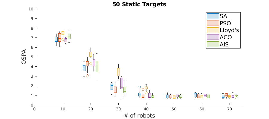
Figure 1: Comparison of steady state median OSPA errors across 10 trials for various distributed control algorithms, considering a range of robot numbers and 50 static targets.

Predicting the trend of system performance at steady state is relatively straightforward, especially when considering single variables. For instance, it is intuitive to assume that an increase in the number of robots or the size of their FoV enhances search and tracking capabilities. Conversely, an increase in the number of targets elevates the required search capacity. However, the situation becomes more complex when multiple variables change simultaneously, particularly when the goal is to predict system performance over time, rather than at steady state. Obtaining a quantitative forecast under these conditions is both more valuable and more challenging.

In this paper, we undertake an analysis based on five parameters across various algorithms: the number of robots ($n_{r}$), the number of targets ($n_{t}$), the radius of the FoV for each robot ($r$), the robot density in the environment ($\rho_{r}$), and the target density in the environment ($\rho_{t}$). We define $\theta$ as the parameter vector containing these variables, formally expressed as $\theta=\left[n_{r},n_{t},r,\rho_{r},\rho_{t}\right]^{T}$. Robot density affects coverage capabilities and the frequency of interactions among robots, which in turn impacts the efficiency of task allocation and the complexity of coordination. Meanwhile, target density determines the difficulty of the tracking task; higher densities may complicate the identification and tracking of individual targets. Considering that the size of the environment may vary for robots and targets, it is necessary to account for these densities separately.

III-C Dataset Collection

This study will address MR-MTT within an open 100$\times$100 m region. All robots start at random locations within a confined box situated towards the lower central region of the map. These robots, which are holonomic, have a maximum velocity of 2 m/s. Each robot is fitted with an onboard sensor providing a circular FoV with a radius ranging from $r=3-7\,\mathrm{m}$. The false negative rate in detection is set at $p_{\rm fn}=0.2$ (i.e., a robot fails to detect a target within its field of view 20% of the time). For each target that is detected, the robot receives a noisy measurement of the relative position, drawn from a normal distribution with 0 mean and covariance $0.25I_{2}$. The sensors record measurements at a rate of 2 Hz. We vary the number of robots in the team and targets in the search space from 10 thru 100, in increments of 10. Targets positions are drawn uniformly at random from within the search space. It is important to clarify that these values do not correspond to a specific real-world scenario but could resemble a drone team equipped with downward-facing cameras. For real-world applications, one could adopt the procedures detailed in our other works to accurately characterize sensor models [chen2022semantic].

For each team/task configuration, we run 10 trials, a number we have found to be representative in our previous studies. This provides us with a large dataset from which we can extract trends.

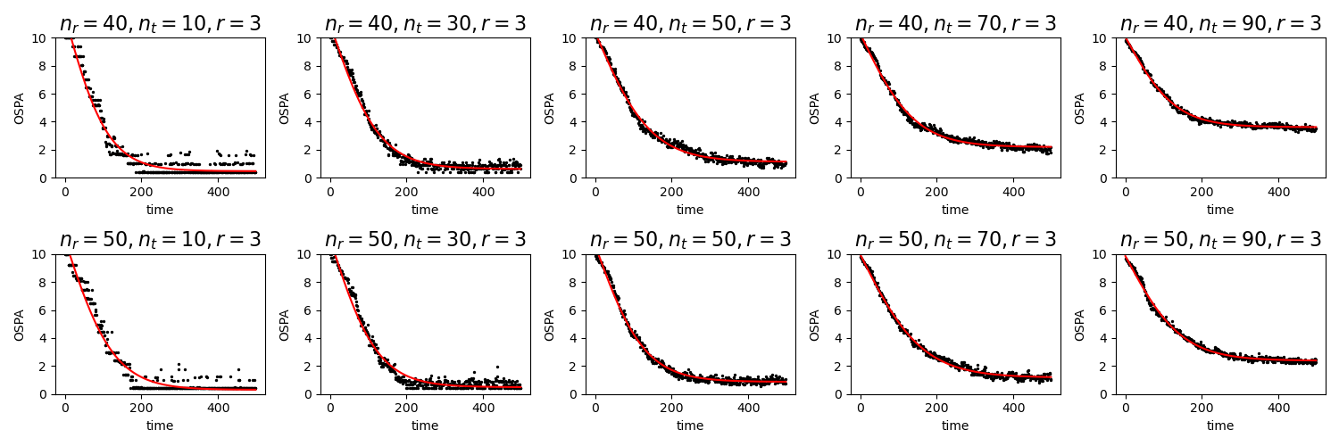
Figure 2: The black points represent the median OSPA value from the dataset with a batch size of 10 over time. The red lines illustrate the fitting results using a sigmoid function.

III-D Performance Metrics

We utilize two performance metrics in our study, one based on tracking error and the other on exploration rate. We measure both transient and steady state performance of the MRS, where we use the median value over the final 50 s as our indicator of the steady-state value. Additionally, we take the median value of the metric across the 10 trials in order to decrease the impact of stochastic error and increasing the reliability of our results. Through this method, we are able to derive discrete data points, subsequently producing a comprehensive dataset.

III-D1 Optimal SubPattern Assignment Metric

The Optimal SubPattern Assignment (OSPA) metric [Schuhmacher2008Metric] is a commonly used metric in the MTT community that measures the average error of all targets. The OSPA between two sets $X,Y$, where $|X|=m\leq|Y|=n$ without loss of generality, is

$$d(X,Y)=\left(\frac{1}{n}\min_{\pi\in\Pi_{n}}\sum_{i=1}^{m}d_{c}(x_{i},y_{\pi(i)})^{p}+c^{p}(n-m)\right)^{\frac{1}{p}}$$ (1)

where $c$ is the cutoff distance, $d_{c}(x,y)=\min(c,\|x-y\|)$, and $\Pi_{n}$ is the set of permutations of $\{1,2,3,...,n\}$. We set $p=1$ as the $p$-norm and use a cutoff distance of $c=10\,\mathrm{m}$. In our case, the two sets $X,Y$ represent the ground truth target set and the estimated target set (from the PHD filter).

Since the OSPA can fluctuate due to false negative and false positive detections, we use the median of the OSPA over the last 50 s of each trial to obtain a steady state estimate in each experiment. From our previous work [xin2022comparing, xin2024comparison], we typically observe a rapid decline in the OSPA value at the outset, which then gradually levels off to a steady value as exploration progresses. Figure 2 shows these trends for different $\theta$ values.

III-D2 Exploration Inefficiency

We also introduce another metric, Exploration Inefficiency ($EI$), which evaluates the percentage of the unexplored area by the robot team over time:

$$EI=\left(1-\frac{\text{Explored Area}}{\text{Total Area}}\right)\times 100\%$$ (2)

This metric will help in evaluating the efficiency of a MRS deployed for environmental monitoring tasks. A lower ($EI$) score suggests that a larger portion of the area has been explored, signifying higher efficiency in monitoring tasks. Therefore, in the context of ensuring comprehensive environmental surveillance, striving for a minimal Exploration Inefficiency percentage is key to maximizing the area monitored by the MRS.

IV Problem Formulation

This section is organized into three parts. Firstly, we introduce the fitting models used to predict the system’s performance over time, where the model parameters are functions of the dimensionless variables. Secondly, we describe the method for generating dimensionless variables from the MRS parameters outlined in the previous section, utilizing the Buckingham Pi theorem. Thirdly, we explain the optimization method employed to determine the parameters for both the fitting model and the generation of dimensionless variables.

IV-A Model Fitting

The objective of deploying fitting models is to succinctly describe the system’s behavior over time using a reduced set of parameters. The general objective function is formulated as follows:

$$\min\sum_{n=1}^{N}\sum_{t=1}^{T}\|\hat{m}(t\mid\theta_{n})-m_{t,n}\|^{2}$$ (3)

where $m_{t,n}$ is the value of the performance metric (OSPA or EI) at time $t$ in training data $n$ and $\hat{m}(t\mid\theta_{n})$ denotes the prediction model for that metric, which depends on the team/task parameters $\theta_{n}$ in the training sequence $n$.

The approach we use is to select a parametric model for $\hat{m}(t\mid\theta_{n})$ and to try to connect the parameters of that model to $\theta_{n}$. This will allow us to predict the performance based on the specific team parameter configurations at any given time. We introduce symbol $\Phi$ to denote the collection of model parameters in $\hat{m}(t\mid\theta_{n})$. Based on our observations in Fig. 2, we will utilize two different models within the exponential family due to their inherent capability to encapsulate the decay present in the data.

The first is an exponential model:

$$\hat{m}(t\mid\Phi(\theta))=ae^{-bt}+c$$ (4)

Here the model parameter set is $\Phi=\{a,b,c\}$, which describe the initial state ($a$), decay rate ($b$), and steady-state behavior ($c$). The second is a sigmoid model:

$$\hat{m}(t\mid\Phi(\theta))=\frac{L}{1+e^{-kt}}+d$$ (5)

Here the model parameter set is $\Phi=\{L,k,d\}$, which describe the maximum value ($L$), the curve’s steepness ($k$), and the baseline adjustment ($d$).

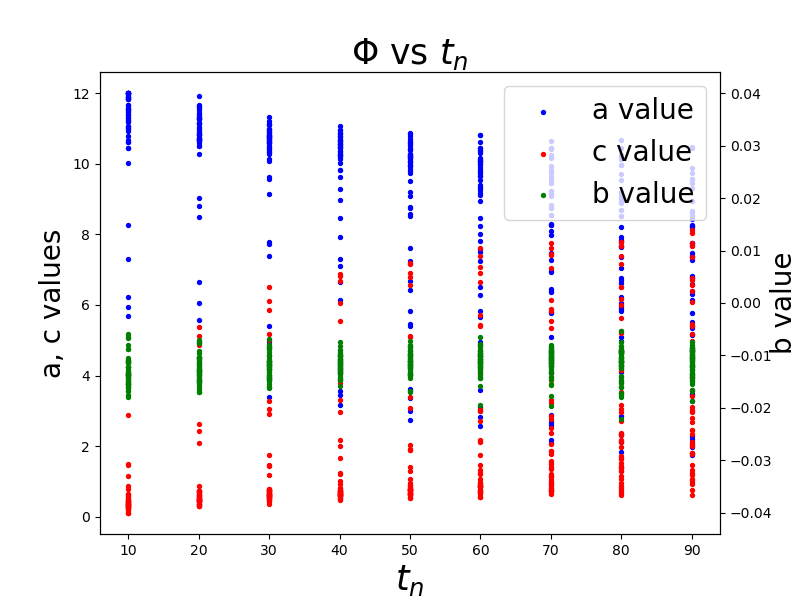
(a) $\Phi=\{a,b,c\}$ vs $n_{t}$

(b) $\Phi=\{L,k,d\}$ vs $n_{t}$

Figure 3: Comparative analyses of the variables $a$, $b$, and $c$ from the Exponential fitting method, and $L$, $k$, and $d$ from the sigmoid fitting method, against the target number $n_{t}$. The data is from ACO method.

These parameters play a critical role in modeling the predictive trajectory of system performance over time, capturing the system’s dynamics effectively. The most straightforward method to predict $\hat{m}(t\mid\Phi(\theta))$ involves first modeling $\Phi(\theta)$ with respect to $\theta$ and then utilizing $\Phi(\theta)$ for prediction. However, early tests indicate that directly modeling $\Phi(\theta)$ with $\theta$ poses challenges. Figures 3a and 3b display the values of the parameters $\Phi$ against the number of targets $n_{t}$, using the exponential and sigmoid fitting methods, respectively. While there is a discernible trend, a large variance in the data makes accurate prediction difficult since you can have vastly different $\Phi$ values for the same $n_{t}$. Similar trends hold for the other parameters within $\theta$.

IV-B Dimensionless Variable Structure

In this section, we propose the formula of a dimensionless variable $\Pi(\theta)$ for the MR-MTT problem. The idea to depict system performance through a dimensionless variable is influenced by preceding research, such as Xie et al. [Xie2022], which utilizes dimensionless variables to model physical laws. Moreover, the study by Kwa et al. [kwa2023effect] also lends inspiration, investigating the correlation between robot density and the phase transition from exploration to exploitation within MRS. The primary benefit of a dimensionless variable $\Pi(\theta)$ is to enable comparisons across different scales.

To find potential dimensionless variables, we first create a dimensional matrix $\mathbf{D}$. In such a matrix, there is a column for each a variable and a row for each type of unit. In our case, we have $n=5$ dimensional variables (from $\Pi=(n_{r},n_{t},r,\rho_{r},\rho_{t})$) with $m=2$ units (item and meter). The entries in row $i$ and column $j$ is the power of unit $i$ in variable $j$, as shown below. For example, we can read column 4 as saying that the variable $\rho_{r}$ has units of quantity per square meter.

$$\begin{array}{cccccc}\hfill 𝐃=\mathrm{𝐜𝐜𝐜𝐜𝐜𝐜}n{}_r& \hfill n{}_t& \hfill r& \hfill \rho {}_r& \hfill \rho {}_t& \\ \hfill [\mathrm{𝐜𝐜𝐜𝐜𝐜}]\mathrm{𝐜𝟏}& \hfill \mathrm{𝟏}& \hfill \mathrm{𝟎}& \hfill \mathrm{𝟏}& \hfill \mathrm{𝟏}& \hfill \text{unit}\\ \hfill \mathrm{𝟎}& \hfill \mathrm{𝟎}& \hfill \mathrm{𝟏}& \hfill -\mathrm{𝟐}& \hfill -\mathrm{𝟐}& \hfill \text{meter}\end{array}\mathrm{𝐀𝐝𝐢𝐦𝐞𝐧𝐬𝐢𝐨𝐧𝐥𝐞𝐬𝐬𝐯𝐚𝐫𝐢𝐚𝐛𝐥𝐞𝐢𝐬𝐨𝐧𝐞𝐬𝐮𝐜𝐡𝐭𝐡𝐚𝐭𝐭𝐡𝐞𝐦𝐮𝐥𝐭𝐢𝐩𝐥𝐢𝐜𝐚𝐭𝐢𝐨𝐧}(\mathrm{𝐚𝐧𝐝𝐝𝐢𝐯𝐢𝐬𝐢𝐨𝐧})\mathrm{𝐨𝐟𝐢𝐭𝐬𝐜𝐨𝐧𝐬𝐭𝐢𝐭𝐮𝐞𝐧𝐭𝐩𝐚𝐫𝐭𝐬𝐡𝐚𝐬𝐧𝐨𝐫𝐞𝐬𝐮𝐥𝐭𝐚𝐧𝐭𝐮𝐧𝐢𝐭𝐬}.\mathrm{𝐈𝐧𝐨𝐮𝐫𝐜𝐚𝐬𝐞},\mathrm{𝐰𝐞𝐬𝐞𝐞𝐤𝐚𝐜𝐨𝐦𝐛𝐢𝐧𝐚𝐭𝐢𝐨𝐧𝐨𝐟𝐭𝐡𝐞𝐜𝐨𝐥𝐮𝐦𝐧𝐬𝐨𝐟}\text{D}\mathrm{𝐬𝐮𝐜𝐡𝐭𝐡𝐚𝐭𝐭𝐡𝐞𝐫𝐞𝐬𝐮𝐥𝐭𝐚𝐧𝐭𝐢𝐬𝐭𝐡𝐞𝐳𝐞𝐫𝐨𝐯𝐞𝐜𝐭𝐨𝐫}(\mathrm{𝐦𝐞𝐚𝐧𝐢𝐧𝐠𝐢𝐭𝐡𝐚𝐬𝐧𝐨𝐮𝐧𝐢𝐭𝐬𝐨𝐟𝐚𝐧𝐲𝐤𝐢𝐧𝐝}).\mathrm{𝐅𝐫𝐨𝐦𝐥𝐢𝐧𝐞𝐚𝐫𝐚𝐥𝐠𝐞𝐛𝐫𝐚},\mathrm{𝐭𝐡𝐢𝐬𝐢𝐬𝐭𝐡𝐞𝐧𝐮𝐥𝐥𝐬𝐩𝐚𝐜𝐞𝐨𝐟}\text{D}.\mathrm{𝐀𝐜𝐜𝐨𝐫𝐝𝐢𝐧𝐠𝐭𝐨𝐭𝐡𝐞𝐁𝐮𝐜𝐤𝐢𝐧𝐠𝐡𝐚𝐦𝐏𝐢𝐭𝐡𝐞𝐨𝐫𝐞𝐦}\text{<cite class="ltx\_cite ltx\_citemacro\_cite">[<span class="ltx\_ref ltx\_missing\_citation ltx\_ref\_self">curtis1982dimensional</span>]</cite>},\mathrm{𝐭𝐡𝐞𝐫𝐞𝐚𝐫𝐞}\text{n - m = 3}\mathrm{𝐯𝐞𝐜𝐭𝐨𝐫𝐬𝐧𝐞𝐜𝐞𝐬𝐬𝐚𝐫𝐲𝐭𝐨𝐬𝐩𝐚𝐧𝐭𝐡𝐞𝐧𝐮𝐥𝐥𝐬𝐩𝐚𝐜𝐞𝐨𝐟}\text{D},\mathrm{𝐫𝐞𝐩𝐫𝐞𝐬𝐞𝐧𝐭𝐞𝐝𝐛𝐲}\text{W}\text{ = [}\text{w\_1}\text{, }\text{w\_2}\text{, }\text{w\_3}\text{]},\mathrm{𝐚𝐬𝐟𝐨𝐥𝐥𝐨𝐰𝐬}:\text{(7)Eq.EquationEqs.Equations7W=[w1,w2,w3]=[-1-1-1100022010001]}\mathrm{𝐓𝐡𝐞𝐬𝐞𝐯𝐞𝐜𝐭𝐨𝐫𝐬𝐟𝐨𝐫𝐦𝐚𝐛𝐚𝐬𝐢𝐬𝐟𝐨𝐫𝐭𝐡𝐞𝐧𝐮𝐥𝐥𝐬𝐩𝐚𝐜𝐞𝐨𝐟}\text{D}.\mathrm{𝐅𝐢𝐧𝐚𝐥𝐥𝐲},\mathrm{𝐰𝐞𝐜𝐚𝐧𝐚𝐬𝐬𝐞𝐫𝐭𝐭𝐡𝐚𝐭𝐚𝐧𝐲𝐥𝐢𝐧𝐞𝐚𝐫𝐜𝐨𝐦𝐛𝐢𝐧𝐚𝐭𝐢𝐨𝐧}\text{w}\mathrm{𝐨𝐟𝐭𝐡𝐞𝐬𝐞𝐛𝐚𝐬𝐢𝐬𝐯𝐞𝐜𝐭𝐨𝐫𝐬𝐰𝐢𝐥𝐥𝐚𝐥𝐬𝐨𝐛𝐞𝐝𝐢𝐦𝐞𝐧𝐬𝐢𝐨𝐧𝐥𝐞𝐬𝐬}:\text{(8)Eq.EquationEqs.Equations8w=γ1w1+γ2w2+γ3w3=[wnr,wnt,wr,wρr,wρt]T}\mathrm{𝐅𝐨𝐫𝐨𝐮𝐫𝐯𝐚𝐫𝐢𝐚𝐛𝐥𝐞𝐬𝐞𝐭}\text{θ},\mathrm{𝐚𝐧𝐲𝐝𝐢𝐦𝐞𝐧𝐬𝐢𝐨𝐧𝐥𝐞𝐬𝐬𝐯𝐚𝐫𝐢𝐚𝐛𝐥𝐞}\text{Π(}\text{θ}\text{)}\mathrm{𝐜𝐚𝐧𝐭𝐡𝐮𝐬𝐛𝐞𝐰𝐫𝐢𝐭𝐭𝐞𝐧𝐢𝐧𝐭𝐡𝐞𝐟𝐨𝐥𝐥𝐨𝐰𝐢𝐧𝐠𝐟𝐨𝐫𝐦𝐬}:\text{(9)Eq.EquationEqs.Equations9}\begin{array}{cc}\hfill 𝚷(\theta ,𝐰)& =𝐧{}_{𝐫}{}^{𝐰{}_{𝐧{}_{𝐫}}}𝐧{}_{𝐭}{}^{𝐰{}_{𝐧{}_{𝐭}}}𝐫{}^{𝐰{}_{𝐫}}\rho {}_{𝐫}{}^{𝐰{}_{\rho {}_{𝐫}}}\rho {}_{𝐭}{}^{𝐰{}_{\rho {}_{𝐭}}}\hfill \\ \hfill 𝚷(\theta ,𝜸)& =\left(\frac{𝐧{}_{𝐭}}{𝐧{}_{𝐫}}\right){}^{\gamma {}_{\mathrm{𝟏}}}\left(\frac{𝐫{}^{\mathrm{𝟐}}\rho {}_{𝐫}}{𝐧{}_{𝐫}}\right){}^{\gamma {}_{\mathrm{𝟐}}}\left(\frac{𝐫{}^{\mathrm{𝟐}}\rho {}_{𝐭}}{𝐧{}_{𝐫}}\right){}^{\gamma {}_{\mathrm{𝟑}}}\hfill \end{array}\mathrm{𝐖𝐞𝐰𝐢𝐥𝐥𝐜𝐚𝐥𝐥}\mathbf{(}\text{<a href="\#S4.E11" title="In IV-B Dimensionless Variable Structure ‣ IV Problem Formulation ‣ Towards Predicting Collective Performance in Multi-Robot Teams" class="ltx\_ref ltx\_font\_bold"><span class="ltx\_text ltx\_ref\_tag">11</span></a>}\mathbf{)}\mathrm{𝐭𝐡𝐞}\text{w}\mathrm{𝐟𝐨𝐫𝐦𝐨𝐟}\text{Π}\mathrm{𝐚𝐧𝐝𝐜𝐚𝐥𝐥}\mathbf{(}\text{<a href="\#S4.E11" title="In IV-B Dimensionless Variable Structure ‣ IV Problem Formulation ‣ Towards Predicting Collective Performance in Multi-Robot Teams" class="ltx\_ref ltx\_font\_bold"><span class="ltx\_text ltx\_ref\_tag">11</span></a>}\mathbf{)}\mathrm{𝐭𝐡𝐞}\text{γ}\mathrm{𝐟𝐨𝐫𝐦𝐨𝐟}\text{Π}.\mathrm{𝐓𝐡𝐞𝐠𝐨𝐚𝐥𝐢𝐬𝐭𝐨𝐥𝐞𝐚𝐫𝐧𝐭𝐡𝐞𝐜𝐨𝐞𝐟𝐟𝐢𝐜𝐢𝐞𝐧𝐭𝐬}\text{γ}\text{ = [}\text{γ}\text{\_1, }\text{γ}\text{\_2, }\text{γ}\text{\_3]^T}\mathrm{𝐭𝐨𝐟𝐢𝐧𝐝𝐚}\mathrm{`}\mathrm{`}\mathrm{𝐮𝐬𝐞𝐟𝐮𝐥}{}^{\prime \prime }\text{Π}\mathrm{𝐭𝐡𝐚𝐭𝐮𝐧𝐜𝐨𝐯𝐞𝐫𝐬𝐬𝐭𝐫𝐮𝐜𝐭𝐮𝐫𝐞𝐢𝐧𝐭𝐡𝐞𝐌𝐑𝐒𝐩𝐞𝐫𝐟𝐨𝐫𝐦𝐚𝐧𝐜𝐞}.\mathrm{𝐀𝐜𝐫𝐮𝐜𝐢𝐚𝐥𝐚𝐬𝐩𝐞𝐜𝐭𝐨𝐟𝐨𝐮𝐫𝐚𝐧𝐚𝐥𝐲𝐬𝐢𝐬𝐢𝐬𝐭𝐡𝐞𝐞𝐱𝐚𝐦𝐢𝐧𝐚𝐭𝐢𝐨𝐧𝐨𝐟𝐭𝐡𝐞𝐬𝐭𝐫𝐮𝐜𝐭𝐮𝐫𝐞𝐨𝐟𝐭𝐡𝐞𝐝𝐢𝐦𝐞𝐧𝐬𝐢𝐨𝐧𝐥𝐞𝐬𝐬𝐯𝐚𝐫𝐢𝐚𝐛𝐥𝐞𝐬𝐰𝐢𝐭𝐡𝐢𝐧𝐭𝐡𝐞𝐬𝐞𝐦𝐨𝐝𝐞𝐥𝐬}.\mathrm{𝐒𝐩𝐞𝐜𝐢𝐟𝐢𝐜𝐚𝐥𝐥𝐲},\mathrm{𝐰𝐞𝐟𝐨𝐜𝐮𝐬𝐨𝐧𝐭𝐡𝐞𝐩𝐨𝐰𝐞𝐫𝐬𝐚𝐬𝐬𝐢𝐠𝐧𝐞𝐝𝐭𝐨𝐞𝐚𝐜𝐡𝐜𝐨𝐦𝐩𝐨𝐧𝐞𝐧𝐭𝐩𝐚𝐫𝐚𝐦𝐞𝐭𝐞𝐫}(\text{w}\mathrm{𝐨𝐫}\text{γ}),\mathrm{𝐰𝐡𝐢𝐜𝐡𝐫𝐞𝐩𝐫𝐞𝐬𝐞𝐧𝐭𝐭𝐡𝐞}\mathrm{`}\mathrm{`}\mathrm{𝐬𝐭𝐫𝐮𝐜𝐭𝐮𝐫𝐞}{}^{\prime \prime }\mathrm{𝐨𝐟𝐭𝐡𝐞𝐝𝐢𝐦𝐞𝐧𝐬𝐢𝐨𝐧𝐥𝐞𝐬𝐬𝐯𝐚𝐫𝐢𝐚𝐛𝐥𝐞}\text{Π(}\text{θ}\text{)}.\mathrm{𝐈𝐟𝐰𝐞𝐟𝐢𝐧𝐝𝐚𝐬𝐢𝐦𝐢𝐥𝐚𝐫𝐬𝐭𝐫𝐮𝐜𝐭𝐮𝐫𝐞𝐫𝐞𝐠𝐚𝐫𝐝𝐥𝐞𝐬𝐬𝐨𝐟𝐭𝐡𝐞𝐟𝐢𝐭𝐭𝐢𝐧𝐠𝐦𝐨𝐝𝐞𝐥𝐮𝐬𝐞𝐝},\mathrm{𝐢𝐭𝐰𝐢𝐥𝐥𝐥𝐞𝐧𝐝𝐠𝐫𝐞𝐚𝐭𝐞𝐫𝐜𝐫𝐞𝐝𝐢𝐛𝐢𝐥𝐢𝐭𝐲𝐭𝐨𝐭𝐡𝐞𝐢𝐝𝐞𝐚𝐭𝐡𝐚𝐭𝐭𝐡𝐞𝐝𝐢𝐦𝐞𝐧𝐬𝐢𝐨𝐧𝐥𝐞𝐬𝐬𝐯𝐚𝐫𝐢𝐚𝐛𝐥𝐞𝐩𝐫𝐨𝐯𝐢𝐝𝐞𝐬𝐦𝐞𝐚𝐧𝐢𝐧𝐠𝐟𝐮𝐥𝐢𝐧𝐬𝐢𝐠𝐡𝐭𝐬𝐢𝐧𝐭𝐨𝐭𝐡𝐞𝐮𝐧𝐝𝐞𝐫𝐥𝐲𝐢𝐧𝐠𝐩𝐞𝐫𝐟𝐨𝐫𝐦𝐚𝐧𝐜𝐞𝐨𝐟𝐭𝐡𝐞𝐌𝐑𝐒𝐬𝐲𝐬𝐭𝐞𝐦}.\text{IV-CSectionSectionSectionsSectionsIV-C§IV-CIV-CProcedureforLea}$$ (11)